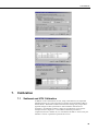
1
USER MANUAL OBS-5+ Turbidity Sensor Issued: 9.12.13 Copyright © 2008-2013 Campbell Scientific, Inc. Printed under licence by Campbell Scientific Ltd. CSL 729 Guarantee This equipment is guaranteed against defects in materials and workmanship. This guarantee applies for twelve months from date of delivery. We will repair or replace products which prove to be defective during the guarantee period provided they are returned to us prepaid. The guarantee will not apply to: Equipment which has been modified or altered in any way without the written permission of Campbell Scientific Batteries Any product which has been subjected to misuse, neglect, acts of God or damage in transit. Campbell Scientific will return guaranteed equipment by surface carrier prepaid. Campbell Scientific will not reimburse the claimant for costs incurred in removing and/or reinstalling equipment. This guarantee and the Company’s obligation thereunder is in lieu of all other guarantees, expressed or implied, including those of suitability and fitness for a particular purpose. Campbell Scientific is not liable for consequential damage. Please inform us before returning equipment and obtain a Repair Reference Number whether the repair is under guarantee or not. Please state the faults as clearly as possible, and if the product is out of the guarantee period it should be accompanied by a purchase order. Quotations for repairs can be given on request. It is the policy of Campbell Scientific to protect the health of its employees and provide a safe working environment, in support of this policy a “Declaration of Hazardous Material and Decontamination” form will be issued for completion. When returning equipment, the Repair Reference Number must be clearly marked on the outside of the package. Complete the “Declaration of Hazardous Material and Decontamination” form and ensure a completed copy is returned with your goods. Please note your Repair may not be processed if you do not include a copy of this form and Campbell Scientific Ltd reserves the right to return goods at the customers’ expense. Note that goods sent air freight are subject to Customs clearance fees which Campbell Scientific will charge to customers. In many cases, these charges are greater than the cost of the repair. Campbell Scientific Ltd, Campbell Park, 80 Hathern Road, Shepshed, Loughborough, LE12 9GX, UK Tel: +44 (0) 1509 601141 Fax: +44 (0) 1509 601091 Email: [email protected] www.campbellsci.co.uk PLEASE READ FIRST About this manual Please note that this manual was originally produced by Campbell Scientific Inc. primarily for the North American market. Some spellings, weights and measures may reflect this origin. Some useful conversion factors: Area: 1 in2 (square inch) = 645 mm2 Length: 1 in. (inch) = 25.4 mm 1 ft (foot) = 304.8 mm 1 yard = 0.914 m 1 mile = 1.609 km Mass: 1 oz. (ounce) = 28.35 g 1 lb (pound weight) = 0.454 kg Pressure: 1 psi (lb/in2) = 68.95 mb Volume: 1 UK pint = 568.3 ml 1 UK gallon = 4.546 litres 1 US gallon = 3.785 litres In addition, while most of the information in the manual is correct for all countries, certain information is specific to the North American market and so may not be applicable to European users. Differences include the U.S standard external power supply details where some information (for example the AC transformer input voltage) will not be applicable for British/European use. Please note, however, that when a power supply adapter is ordered it will be suitable for use in your country. Reference to some radio transmitters, digital cell phones and aerials may also not be applicable according to your locality. Some brackets, shields and enclosure options, including wiring, are not sold as standard items in the European market; in some cases alternatives are offered. Details of the alternatives will be covered in separate manuals. Part numbers prefixed with a “#” symbol are special order parts for use with non-EU variants or for special installations. Please quote the full part number with the # when ordering. Recycling information At the end of this product’s life it should not be put in commercial or domestic refuse but sent for recycling. Any batteries contained within the product or used during the products life should be removed from the product and also be sent to an appropriate recycling facility. Campbell Scientific Ltd can advise on the recycling of the equipment and in some cases arrange collection and the correct disposal of it, although charges may apply for some items or territories. For further advice or support, please contact Campbell Scientific Ltd, or your local agent. Campbell Scientific Ltd, Campbell Park, 80 Hathern Road, Shepshed, Loughborough, LE12 9GX, UK Tel: +44 (0) 1509 601141 Fax: +44 (0) 1509 601091 Email: [email protected] www.campbellsci.co.uk Contents PDF viewers: These page numbers refer to the printed version of this document. Use the PDF reader bookmarks tab for links to specific sections. 1. Introduction ................................................................ 1 2. Cautionary Statements .............................................. 1 3. Initial Inspection ........................................................ 1 3.1 Ships With ............................................................................................ 1 4. Overview ..................................................................... 2 4.1 4.2 Optics ................................................................................................... 2 SSC-Measurement Principle ................................................................ 3 5. Specifications ............................................................ 5 5.1 5.2 5.3 5.4 5.5 Measurement Range ............................................................................. 5 Accuracy .............................................................................................. 6 OBS-5+ Sensor .................................................................................... 6 Other Data ............................................................................................ 6 Dimensions........................................................................................... 6 6. Operation .................................................................... 7 6.1 Instrument Setup .................................................................................. 7 6.1.1 Mounting Suggestions ................................................................... 7 6.1.2 Surveys .......................................................................................... 7 6.1.3 Logging Data ................................................................................ 8 6.1.4 Battery Installation ........................................................................ 8 6.2 OBS-5+Utility Software....................................................................... 9 6.2.1 Software Installation ..................................................................... 9 6.2.2 Running the OBS-5+ Utility ......................................................... 9 6.2.3 Pull-Down Menus ....................................................................... 11 6.2.4 Communication Settings ............................................................. 11 6.2.5 Testing Sensors ........................................................................... 12 6.2.6 Monitoring Turbidity (NTU)....................................................... 13 6.2.7 Water Density and Barometric Corrections ................................ 13 6.2.8 Sample Statistics ......................................................................... 13 6.2.9 Sampling Modes and Terms........................................................ 14 6.2.10 Surveying .................................................................................... 15 6.2.11 Cyclic Sampling .......................................................................... 16 6.2.12 Data Retrieval ............................................................................. 17 6.2.13 Shutdown .................................................................................... 18 6.2.14 Graphing and Printing ................................................................. 18 6.2.15 Excel Spreadsheets ...................................................................... 18 i 7. Calibration ................................................................ 19 7.1 Sediment and NTU Calibration .......................................................... 19 7.1.1 General Guidance........................................................................ 20 7.1.2 Equipment and Materials ............................................................ 23 7.1.3 Procedure for Sediment ............................................................... 23 7.2 Turbidity (NTU) Calibration .............................................................. 26 7.2.1 Equipment and Materials ............................................................ 26 7.2.2 Procedure for Turbidity............................................................... 26 8. Troubleshooting ...................................................... 28 9. Maintenance ............................................................. 30 9.1 9.2 9.3 9.4 9.5 OBS-5+ Sensor .................................................................................. 30 Pressure Sensor .................................................................................. 30 Batteries ............................................................................................. 30 Pressure Housing................................................................................ 31 User-Serviceable Parts ....................................................................... 31 10. Interfering Factors ................................................... 31 10.1 10.2 10.3 Particle Size ....................................................................................... 32 NIR Reflectivity ................................................................................. 33 Particle Shape, Flocculation, and Disaggregation .............................. 34 11. References ............................................................... 36 Appendix A. Turbidity Standards ............................................... A-1 Figures 4-1. Dimensions (top), sensor endcap with copper antifoulant (Cu a.f.) collars (left) and connector endcap (right) ........................................ 2 4-2. Schematic of optical system ................................................................. 3 4-3. Sample calibration curves (fine and bold lines), lookup tables I, II, and III (bold curves), and sediment concentrations pf ND (open arrow) and FD (solid arrow) peaks. ........................................ 4 4-4. Calibration curves for four different sediments and SSC values for near-detector peaks (coloured arrowheads). ..................................... 5 6-1. Electrical connections .......................................................................... 8 6-2. Battery installation: A) endcap removal, B) wiping, C) cable disconnect, and D) battery contact.................................................... 9 6-3. New data log prompt .......................................................................... 10 6-4. Designating your own file name and destination ............................... 10 7-1. Manual (left) and automatic (right) sediment suspenders .................. 20 7-2. Lookup tables and table limits (a, b, and c)........................................ 21 7-3. OBS-5+ in big black tub of clean water ............................................. 24 7-4. OBS-5+ in suspender tub ................................................................... 25 7-5. OBS-5+ in 100 mm cup ..................................................................... 27 8-1. Internal components ........................................................................... 29 10-1. Effects of sediment size ..................................................................... 33 10-2. Near-infrared reflectivity of minerals ................................................ 34 10-3. Effects of disaggregation methods ..................................................... 35 ii Tables 6-1. 7-1. 7-2. 9-1. 10-1. Working and Maximum Depths ........................................................... 7 Schedule of Concentrations for Sediment Calibrations ...................... 22 SSC-Calculation Spreadsheet ............................................................. 22 Battery Life in Hours with 100% Power ............................................ 31 Relative magnitude of the effects of sediment characteristics on OBS-5+ sensitivity ......................................................................... 32 iii iv OBS-5+ Turbidity Sensor 1. Introduction The manual describes the features of the OBS-5+®, as well as its use for surveys and battery-powered, internal-storage operations. Using backscatter from a 780 nm laser diode and a patented dual-detection system (U.S. Patent Number 5,796,481), a calibrated OBS-5+ measures suspended sediment concentrations, suspended solids concentration (SSC), as large as 200 g L–1, which is about 10 times higher than standard OBS technology. Before installing the OBS-5+, please study: 2. 3. Section 2, Cautionary Statements Section 3, Initial Inspection Cautionary Statements Although the OBS-5+ is rugged, it should be handled as a precision scientific instrument. Maximum depth for the OBS-5+ is limited by the installed pressure sensor. If the maximum depths are exceeded, the pressure sensor will rupture and the housing will flood. See Section 6.1, Instrument Setup, for more information. Always orient the unit so that the OBS-5+ sensor “looks” into water clear of reflective surfaces. Pad the end caps that contact metal with electrical tape, neoprene, or expanded polyethylene tubes. Never mount the instrument by its end caps or attach anything to them. This could a cause a leak. Always put the OBS-5+ in sleep mode when it will not be used for a while to conserve battery capacity (see Section 6.2.13, Shutdown). Initial Inspection 3.1 Upon receipt of the OBS-5+, inspect the packaging and contents for damage. File damage claims with the shipping company. Check this information against the shipping documents to ensure the correct product is received (see Section 3.1, Ships With). Ships With #21304 Accessory Kit #20919 Software Support CD ResourceDVD 1 OBS-5+ Turbidity Sensor 4. Overview Figure 4-1 shows the dimensions of the OBS-5+, the sensors in the sensor end cap, and underwater connection. Detailed specifications are provided in Section 5, Specifications. The OBS-5+ can be operated in Survey or Cyclic Modes. In Survey Mode, the unit sends data via RS-232 or RS-485 to a PC at two hertz, and in Cyclic Mode, it logs as many as 200,000 scans of time, date, depth, and g L–1 in flash memory (one sample per hour for 23 years). When sampling continuously, the unit will run about 125 hours on three C-size alkaline batteries in 20ºC water (about two weeks of eight-hour survey days). When using the instrument for surveys, the data are captured by a PC running the OBS-5+ software. Pressure is measured with a silicon strain-gauge pressure sensor and the depth of the instrument is calculated from water density and barometric pressure entered by the operator. Figure 4-1. Dimensions (top), sensor end cap with copper antifoulant (Cu a.f.) collars (left) and connector end cap (right) 4.1 Optics The heart of the OBS-5+ is an optical system comprised of a near infrared (NIR) laser diode and a photo detector positioned 10 mm from the laser, called the near detector (ND), and one mounted 25 mm from the laser, called the far detector (FD), see Figure 4-2. The detector acceptance-cone angle is 55º, which means that photons must enter the detector sapphire windows at angles less than 27.5º to be detected. The laser light is collimated to a 3 mm by 1 mm elliptical beam with convergence < 2.5 mrad. The angle between the NIR beam and detector acceptance-cone axes is 45º. The OBS-5+ can detect light scattered by particles illuminated by the NIR beam at angles between 105º to 165º. With its automaticpower-control circuit, the laser diode provides stable optical power over time and the 0 to 30ºC operating temperature range. 2 User Manual Figure 4-2. Schematic of optical system 4.2 SSC-Measurement Principle In Figure 4-2, suspended particles scatter light from the NIR beam onto the near and far detectors, and suspended solids concentration (SSC) is estimated with signals counts from these detectors by a microcontroller, using a set of logic rules and lookup tables derived from calibration data. Counts are the digital equivalents of the ND and FD signals and are proportional to backscatter intensity. Sample calibration curves relating ND and FD counts to sediment concentration in g L–1 are shown on Figure 4-3. As particle concentration increases from 0, the ND and FD signals rise to maxima at peak concentrations, shown by the red (open) and blue (solid) arrowheads above the x axis. Beyond the peak sediment concentrations, light attenuation is the dominant factor controlling the light level at the detectors, and so the ND and FD counts decline. The scattered NIR must travel farther to be detected by the FD than by the ND, and therefore the peak of the FD curve occurs at a lower sediment concentration than the peak of the ND curve. The instrument exploits these peak offsets to estimate sediment concentration. Using either the ND or FD counts, whichever is indicated by the logic rules, the microcontroller does a spline interpolation between calibration values to derive an SSC value. It then combines this value with time and pressure data, and sends the results to a PC. 3 OBS-5+ Turbidity Sensor Figure 4-3. Sample calibration curves (fine and bold lines), lookup tables I, II, and III (bold curves), and sediment concentrations pf ND (open arrow) and FD (solid arrow) peaks. The concentrations associated with the ND and FD peaks depend on sediment characteristics as shown by the variety of response curves and the coloured arrowheads on Figure 4-4. Other sediment characteristics being equal, such as shape and NIR reflectivity (see Section 10, Interfering Factors), larger particles produce higher peak concentrations and greater OBS-5+ measurement ranges than smaller particles. 4 User Manual Figure 4-4. Calibration curves for four different sediments and SSC values for near-detector peaks (coloured arrowheads). 5. Specifications Features: 5.1 Connects directly to a PC—no datalogger needed Operates up to six months on three C-cell batteries Monitors high sediment concentrations (up to 200g/L) Logs depth, wave height, wave period, temperature, and salinity Records 200,000 scans of data in the OBS-5+ flash memory Measurement Range Mud (D50=20μm): 0 to 50,000 mg/l Sand (D50=250μm): 0 to 200,000 mg/l Pressure1: 0 to 10, 20, 50, 100, or 200 m Turbidity: 0.4 to 1,000 NTU 5 OBS-5+ Turbidity Sensor 5.2 5.3 5.4 5.5 Accuracy Mud: 2.0% of reading Sand: 4.0% of reading Pressure: 0.5% of full scale Turbidity: 1.5% of full scale OBS-5+ Sensor Laser wavelength: 780 nm Scattering angles (clean water): 105º to 165º Drift over time: <30 ppm per month Drift over temperature: <200 ppm per ºC Other Data Maximum sampling rate: 25 Hz Maximum data rate: 2 Hz Data capacity: 8 MB/200,000 lines Battery capacity: 8Ah Maximum battery life2: 3,000 hrs External supply voltage: 6 to 18 Vdc External supply current: 55 mA Serial-data protocols: RS-232 & RS-485 Maximum housing depth: 300 m (984 ft) Operating temperature range: 0º to 40ºC Storage temperature range: –20º to 70ºC Dimensions Length / diameter: 380 mm (15 in) / 60 mm (2.4 in) Weight: 2.04 kg (4.5 lb) Weight (submerged): 1.02 kg (2.3 lb) 1 2 6 Range depends on pressure sensor option chosen. Sampling interval is two hours and duration is two minutes. User Manual 6. Operation 6.1 Instrument Setup 6.1.1 Mounting Suggestions CAUTION Maximum depth for the OBS-5+ is limited by the installed pressure sensor. If the maximum depths are exceeded, the pressure sensor will rupture and the housing will flood. The depth limits are listed in Table 6-1. Table 6-1. Working and Maximum Depths Pressure Sensor Working Depth Maximum Depth 5 Bar 0 to 50 metres 75 metres 10 Bar 0 to 100 metres 150 metres 20 Bar 0 to 200 metres 300 metres (1 Bar = 10 dBar ≅ 10 metres of fresh water) The following precautions should be followed to ensure the unit can function properly and is not lost or damaged. Always orient the unit so that the OBS-5+ sensor “looks” into water clear of reflective surfaces. Pad the end caps that contact metal with electrical tape, neoprene, or expanded polyethylene tubes. Never mount the instrument by its end caps or attach anything to them. This could a cause a leak. 6.1.2 Surveys The OBS-5+ will usually be towed with a cable harness for surveys. The serial cable can tow the OBS-5+ without a depressor weight or vane as long as the connector is strain relieved. Strain relief can be provided by attaching the cable to the stainless steel housing (Figure 4-1) with a cable grip and a length of 3 mm (1/8 in) wire rope. Install a cable clamp with a 0.5 m wire rope to the serial cable, and clamp the wire rope to the pressure housing with two stainless steel hose clamps, providing a small loop of slack cable to absorb towing forces. The unit can be powered with an external battery, as shown on Figure 6-1, and the serial output can be transmitted by either RS-232 or RS-485 protocols. The latter protocol is recommended for cable lengths greater than 25 m. An RS-485/232 serial converter is provided with each unit. An RS-232 to USB converter is an available option. 7 OBS-5+ Turbidity Sensor 8 6 6 – 18 V d.c. (Red) Power GND (Black) DB-9 7 5 4 3 8 4, 1, 5, 6, 9 DB-9 3 2 6 2 3 5 (RS485) (A) (B) (GND) (RS232) (RD) (TD) (GND) Figure 6-1. Electrical connections 6.1.3 Logging Data In applications where a survey cable is impractical or when the OBS-5+ must be attached to an instrument frame, it can be powered by the internal batteries and the data can be logged by the data flash memory. See instructions for Cyclic Mode sampling in Section 6.2.11, Cyclic Sampling. 6.1.4 Battery Installation Remove the set screws from the end cap with the handle and connector. If the unit was submerged during the previous day, turn the sensor end up, so water around the O-rings can drain out when the end cap is removed, Figure 6-2 (A). Pull end cap out and disconnect the inline connector (B). Wipe water from the inside wall of the housing tube with a paper towel (C). Turn the connector end up and push the ridge on the battery sliding contact until the spent batteries pop out (D). Insert new batteries with the positive terminal (+) toward the sliding contact. Push the batteries down and slide the contact over the top of them and against the housing wall. Inspect the O-ring in the cap, clean and grease or replace it if necessary, and replace the cap and set screws. For extended deployment time, lithium batteries are a good alternative to alkaline batteries. Campbell Scientific sells a C-cell-sized battery spacer (pn #21905) that allows lithium C-cell batteries to be used with the OBS-5+. Lithium C-cell batteries have a higher voltage than their alkaline counterparts, necessitating the spacer. Campbell Scientific does not sell lithium C-cell batteries. 8 User Manual Figure 6-2. Battery installation: A) end cap removal, B) wiping, C) cable disconnect, and D) battery contact 6.2 OBS-5+Utility Software 6.2.1 Software Installation Insert the CD and select “Install OBS-5+ Utility”. Follow the installation wizard to install the software. The OBS-5+ Utility is the GUI interface with the OBS-5+. As part of the installation, there are several additional files included. This section explains how to program and operate the unit with the OBS-5+ Utility. It covers: 1) turning the OBS-5+ ON and OFF and testing the sensors, 2) selecting sensors and data statistics, 3) scheduling data logging, 4) recording data with a PC or uploading data from the OBS-5+, 5) importing data into a spreadsheet, and 6) plotting data with OBS-5+ Utility. 6.2.2 Running the OBS-5+ Utility 1) Set PC to the time standard for your project. 2) Select the OBS-5+ program to start the OBS-5+ Utility and open the Data Window and Toolbar with the View pull-down menu. 3) The OBS-5+ Utility will create a new data log file and prompt you to accept the name (see Figure 6-3). Files are automatically named with Greenwich Date and Time as follows: OBS5+_20010808_172433.log. Or you can create your own file name and destination by choosing No (see Figure 6-4). Data 9 OBS-5+ Turbidity Sensor received from the OBS-5+ while it is connected to the PC will be stored in this file. Figure 6-3. New data log prompt Figure 6-4. Designating your own file name and destination 4) Connect the OBS-5+ to a PC with the test cable (Figure 6-1). 5) Click Connect/Disconnect to get a green light and synchronize the OBS- 5+ clock with your PC by clicking 10 . User Manual 6.2.3 Pull-Down Menus The OBS-5+ Utility has four pull-down menus for File, OBS-5+, View, and Help. The File menu allows you to select the location and formatting for OBS-5+ files. Files can be opened as plots or ASCII text that can be brought into spreadsheet programs or text editors. Plot files display OBS-5+ data graphically in the main GUI window. The OBS-5+ menu is used to: 1) put the instrument into a low-power Sleep, 2) wake it up if it is sleeping (Wakeup), 3) make a Barometric Correction (see Section 6.2.7, Water Density and Barometric Corrections), 4) view a list of calibration tables, 5) set detector gains (Set Gains), 6) Retrieve an Active Table, 7) Retrieve detector Gains, or 8) switch to RS-485 serial communication. The View menu controls the display on your PC. Switches are provided for: Toolbar toggles the icons ON and OFF. Status Bar toggles the status bar at the bottom of the screen ON or OFF. Data Window pops the data window into view. 6.2.4 Communication Settings The Plot and Port Settings button has a serial port tab for configuring the communication settings. The default settings are: 115 kB, 8 data bits, no parity, no flow control. These settings will work for most applications and with most PCs. In order to pick a slower baud rate and avoid data-transfer errors, select the desired rate from the dialog box and click Apply. The rate adjustment takes two seconds. If your PC is set to the wrong rate for some reason, use the check box to select ONLY change host computer port. Then click Apply and the Settings button. OBS If you get the OBS-5+ information box, the baud rate of the unit is synchronized with your PC. If you don’t get an information box, repeat the above procedure until communication is established. 11 OBS-5+ Turbidity Sensor 6.2.5 Testing Sensors 1) Before daily operations and deployments, verify that the instrument works by clicking Open Plot, and then clicking Survey. Select all sensors and click Start Survey. An example plot of data is shown below. 2) Wave your hand in front of the OBS-5+ sensor; the turbidity and SSC levels on the top plot will fluctuate as data scrolls across the plot. 3) Blow into the pressure sensor or press your thumb on it to compress air on the diaphragm (Figure 4-1). A small elevation in the pressure signal will occur (bottom plot). 4) Click Stop and then OBS Settings to view time, serial numbers, depth corrections, and software versions. 12 User Manual 6.2.6 Monitoring Turbidity (NTU) The OBS-5+ was calibrated and factory-certified using AMCO Clear, U.S. EPAapproved turbidity standards (www.gfschemicals.com). In order to measure turbidity, the electronic gain of the near detector is set to the calibration value and the active lookup table is overridden. Consequently, the unit cannot simultaneously measure SSC (g L–1) and NTU when either g L–1 or NTU is selected. You must choose one or the other. 6.2.7 Water Density and Barometric Corrections Instrument depth is estimated from pressure and it is important to set the water temperature and salinity so the OBS-5+ can correct for water density and calculate depth correctly. The sensor measures absolute pressure so the instrument must also correct for barometric pressure. Be sure to do this while the OBS-5+ is at the surface. Depending on the magnitude of barometric pressure fluctuations at the site and the desired accuracy, you may want to correct data for atmospheric effects using barometric pressure simultaneously recorded at a nearby site. 6.2.8 Sample Statistics The individual measurements are not recorded in the data flash memory and you must select the sample statistics that will be recorded. Two types of statistics can be selected for OBS-5+ measurements. 1) Measures of central tendency, including the mean and median. 2) Measures of variation or spread in sample values, including the standard deviation (σ) and cumulative percentages, such as X25 and X75 (where X is the depth, SSC, or NTU values). The mean is the arithmetic average of the values (∑ x / n), where ∑ x is the sum of the sample values (x) and n is the number of values (sample size). The median (X50) is the value that exceeds 50% of the sample values and is the best measure of central tendency when a sample has outliers. The percentages X25, X50, X75, etc., exceed 25, 50, and 75% of the sample values. 13 OBS-5+ Turbidity Sensor 6.2.9 Sampling Modes and Terms The following terms concern OBS-5+ sampling schedules. Interval: The time in seconds between the start of one sample and the beginning of the next. The interval must be longer than the duration to allow for statistical computations and data storage. The computer will prompt you if you select an interval that is too short. Duration: This is the length of time in seconds that the OBS-5+ will measure its sensors. The duration must always be less than the interval. The minimum duration is five seconds and the maximum is 2,048 seconds (0.57 hour). Rate: Rate is the frequency of sampling for the duration of measurements. All sensors are sampled at the same rate, typically 2, 5, 10, or 25 times per second (Hz). Power: This indicates the percentage of time over the duration of a sample that sensors are ON. Higher power levels mean larger samples and better statistics, but shorter battery life. Lower levels spare the batteries but result in more random noise in sample statistics (lower signal-to-noise ratios, SNR) Sample Size: The number of measurements made by a sensor in each interval; sample size equals rate times duration. The main factors to consider when setting up OBS-5+ Cyclic sampling schedules include: Sampling interval needed to characterize the processes of interest (for example, water level fluctuations, flood and transport duration, tidal conditions, dredge operations, etc.). Maximum sediment concentration. Statistical requirements, such as sample size and sampling rates. Battery capacity. The goal is to pick a sampling scheme that gets essential information about the process of interest without taking too many samples or sampling too often. Inefficient sampling produces excessive battery consumption and a data avalanche with unnecessary processing. Sampling schedules are set with the Interval, Duration, and Rate parameters. Interval sets how often data are recorded. Select the longest interval that will show the changes in turbidity and water depth that you wish to investigate. Rate sets measurement frequency. The quicker turbidity and depth change, the higher the sampling rate should be to get a stable average value for a sample. Finally, Duration sets how long sensor outputs will be averaged. For example, with an interval of 30 seconds and a duration of five seconds, the OBS-5+ will make measurements for five seconds starting every 30 s. The sample size would be 5 x 25 = 125 measurements for a rate of 25 Hz. Always select duration and rate to give a sample size of at least 30, and to reduce random sampling noise below 50% of its maximum value, select them to give a size greater than 200. Survey: Select the survey mode when operating the unit with a cable connection to a PC and when high data rates are desired. Data can be logged with a PC at rates up to 120 lines per minute (2 Hz). 14 User Manual Cyclic Sampling: Use cyclic sampling to record data internally in the 8 MB, flash memory at regular intervals; for example, every 1, 5, 15, or 30 minutes. Depending on the number of sensors measured and the statistics selected, the OBS-5+ can log as many as 200,000 lines of data, one per hour for 23 years, including time, date, depth, NTUs, and SSC. 6.2.10 Surveying Click the OBS-5+ menu and select Barometric Correction. CAUTION Do not do this while the OBS-5+ is submerged. The OBS-5+ takes about five seconds to measure the surface pressure and compute a barometric correction. 1) Connect the OBS-5+ to PC with survey cable and start OBS-5+ Utility. 2) Open the Data Window with the View pull-down menu. 3) Click the lookup table icon and select a calibration table for your survey. The last active table will be used otherwise. 15 OBS-5+ Turbidity Sensor 4) Click Survey to select: sensors, lines per minute, and depth units (Metres or Feet). Set temperature and salinity for the survey area. 5) Click Start Survey and check the data flow in the Data Window. 6) A file for logging data was created when you started the OBS-5+ Utility. You can review data at any time with Open and import the log file directly into an Excel spreadsheet for post-survey processing and plotting (see Section 6.2.15, Excel Spreadsheets). 6.2.11 Cyclic Sampling This mode is for logging data at regular intervals such as 1, 10, 15, 30, etc. minutes, for example. 1) Request Barometric Correction from the OBS-5+ menu. Be sure to do this while the OBS-5+ is at the surface (see Section 6.2.10, Surveying ). 2) Open the Data Window with the View pull-down menu. 3) Activate the lookup table for your survey area with activate buttons (Step 3, Section 6.2.10, Surveying). 16 and User Manual 4) Click Cyclic Sampling and select sensors, statistics, depth units (meters or feet), water temperature, and salinity. 5) Select Interval, Duration, Rate, and Power level; see recommendations in Section 6.2.9, Sampling Modes and Terms. 6) Click Start Sampling to begin logging data and watch a few lines as they are displayed in the data window to be sure the schedule is what you want. Unplug test cable; install dummy plug and locking sleeve. The instrument is ready for deployment. 6.2.12 Data Retrieval 1) Remove dummy plug and connect OBS-5+ to PC with test cable (Figure 6-1). 2) Run OBS-5+ Utility. 3) Open the Data Window to verify that the instrument is transmitting data. 4) Click file. to end data collection and use Offload Data to save data in a 5) Highlight the data with the start and end times you want. 6) Click Browse, select a destination file and click OK. 7) Wait for the progress bar to disappear and examine data as a plot or text file (see Section 6.2.5, Testing Sensors). 17 OBS-5+ Turbidity Sensor 6.2.13 Shutdown From the OBS-5+ menu, select Sleep. 6.2.14 Graphing and Printing 1) Use File menu to select how the data file will be opened. 2) Click Open and select a file to view. Print will print a graph when Open As Plot is selected. To print a text file, select Open As Text, and use the Word Pad file print functions. For spreadsheet operations, see the next section. The looks. Plot and Port Settings is used for setting up your plot 3) Use the Min and Max and Sample Range (End and Start) values to bracket the data you need on the graph. Plot Width allows the graph to be sized to fit a PC screen. On the depth plot, select Max = 0 and Min = the maximum depth to display depth increasing downward. 6.2.15 Excel Spreadsheets To make an Excel spreadsheet from OBS-5+ data, start Excel and set file type to All. Open a data file and select Delimited in Step 1 of 3 of the Text Import Wizard. Click Next > and select the delimiter Space; check Treat consecutive delimiters as one; and {none} for Text qualifier. In Step 3 of 3, select the General Column data format and click Finish. 18 User Manual 7. Calibration 7.1 Sediment and NTU Calibration In addition to the concentration, the size, shape, and reflectivity of suspended sediment particles vary from one location to another and will influence OBS-5+ measurements. When these sediment characteristics change, they will produce apparent changes in SSC by themselves unless sediment calibrations are performed. All sediments produce a unique set of calibration curves like the examples shown in Figure 4-4. The sediment calibration procedure is complicated, and for a modest fee, we will calibrate an OBS-5+ sensor with your sediment. Call for a quotation to perform this service. 19 OBS-5+ Turbidity Sensor Figure 7-1. Manual (left) and automatic (right) sediment suspenders 7.1.1 General Guidance The OBS-5+ uses response curves from the near and far detectors to create three lookup tables like those shown on Figure 4-3 and Figure 7-2. The objective of sediment calibration is to create lookup tables from the sediment you will monitor. The OBS-5+ can store lookup tables for as many as 14 sediments. The fifteenth table is reserved for auto-saved archives. To view a calibration table, click button (step 3 in Section 6.2.10, Surveying), highlight a table number and click on the Activate button; then click View Active. The calibration data table contains all the information needed by the OBS-5+ to interpolate SSC values from the detector signals. From left to right, the column lists: 1) SSC values (g L–1), 2) ND counts, 3) 2nd derivatives for ND curve, 4) FD counts, and 5) 2nd derivatives for FD curve. During a calibration, the first table, highlighted in red, is created from the rising limb of the near detector response between zero counts and point “a” (Figure 7-2). The second table, bold blue curve, is used for mid-range SSC values. It is derived from the descending limb of the far detector curve between points “a” and “c”. High SSC values are estimated from a third lookup table, indicated by the bold green line and point “b”, and are derived from the descending limb of the near detector curve. A calibration consists of a set of 15 to 30 calibration points that each includes an SSC value, a near detector count, and a far detector count. 20 User Manual Figure 7-2. Lookup tables and table limits (a, b, and c) Six to ten calibration points are needed to define each table. For the lookup tables to function properly, the peaks in the ND and FD curves must be within ± 2,500 counts of one another, and to maximize resolution, the peak heights should be between 62,000 and 64,500 counts. Start with the schedule shown in Table 7-1 and adapt it to your sediment as required during the calibration procedure. Sediment preparation is a critical factor in calibration quality. Use dry material whenever possible because it can be accurately weighed. Keep in mind that mixing, grinding, and sieving can produce smaller sediment than you will measure in the field and that the OBS-5+ is very sensitive to particle size (see Section 10, Interfering Factors). This means that disaggregation can produce measurement errors. Vigorous disaggregation with a sonic probe, for example, can produce smaller particles that result in more ND and FD counts per unit of SSC than less aggressive methods. An OBS-5+ calibrated with the former material will underestimate SSC in the field. 21 OBS-5+ Turbidity Sensor Table 7-1. Schedule of Concentrations for Sediment Calibrations MUD (D60 < 62 µm) Sand (D60 > 62 µm) Low SSC (0-5 g/l) Midrange (5-20 g/l) High SSC (> 20 g/l) Low SSC (0-10 g/l) Midrange (10-40 g/l) High SSC (> 49 g/l) 0.0 5 25 0.0 12 50 1.0 6 30 2.0 14 60 1.5 7 40 3.0 15 70 2.0 8 50 4.0 20 80 2.5 9 60 5.0 25 90 3.0 10 6.0 30 100 3.5 15 8.0 35 140 4.0 20 10.0 40 160 The operator can control the electronic gain of the detector circuits to optimize the instrument for his sediment. This can be done with the ND Gain and FD Gain boxes in the OBS-5+ program during the calibration using the + and – buttons to toggle gain up or down. The unit automatically scales all calibration counts to match the selected gain. Set the initial ND and FD gain values to 16, starting with the third SSC value in Table 7-2, adjust the gain to keep the ND and FD counts in the range of 50,000 to 60,000. CAUTION While calibration points can be deleted at any time, never start a new SSC value until you are satisfied with the current values and gain setting. The FD counts will peak first at around 2 to 7 g L–1 and the ND will peak between 5 to 20 g L–1. Set the water volume and sediment density for your calibration in cells D1 and E1 (default volume and density are 3.0 l and 2,650 g L–1). Every time sediment is added to the suspender, enter the grams added to column A and read the current SSC value in column C. Table 7-2. SSC-Calculation Spreadsheet A Grams Added B Total Grams C Cs (g/l) (g/l) D Water Volume (l) E Sediment Density (g/l) 1 0.00 0.00 0.00 3.0 2650 2 1.00 1.00 0.33 2 2.00 3.00 1.00 3 3.00 6.00 2.00 4 4.00 10.00 3.33 Sediment concentrations can also be calculated manually with the following equations: 22 User Manual M s Sediment mass (g) g/l Ms M Vi s s Vi Initial volume (liters) s Sediment density (usually 2.65 x 10³ g/l) 7.1.2 Equipment and Materials Dry, completely disaggregated bottom sediment or suspended matter from the monitoring site Large black, neoprene or polyethylene tub 1-gallon (4 l) brown Nalgene polypropylene bottle with top cut off 1-liter volumetric flask Hand-drill motor (manual suspender) Mixing propeller (manual suspender) Scale with 10 mg accuracy Automatic suspender (optional) Tea cup with round bottom and teaspoon 7.1.3 Procedure for Sediment 1) Put batteries in the OBS-5+ and connect it to a PC with test cable using the RS-232 plug (Figure 6-1). 2) Start OBS-5+ Utility program; wake the OBS-5+; and click the Settings button to verify its response. OBS 3) Click the button to view the list of lookup tables stored in the unit. Select an EMPTY Table number for the sediment calibration. 4) Start the calibration with the button and secure the unit in a big black tub filled with clean tap water (Figure 7-3). The sediment-calibration dialog will appear (the initial display will not show the red and green symbols). 23 OBS-5+ Turbidity Sensor Figure 7-3. OBS-5+ in big black tub of clean water 5) Enter 0.001 in the value box and click the Record button to log the clearwater data point. The unit will take 1,200 measurements in 60 seconds. When the process is complete, the data appear in the data table and the ND (red) and FD (green) points will be plotted on the calibration graph. If you are satisfied with the data, mount the unit in the suspender. 6) Position the OBS-5+ so that it produces the minimum FD signal in clear water (Figure 7-4). 24 User Manual Figure 7-4. OBS-5+ in suspender tub 7) Weigh the first increment of sediment with the electronic balance (see Table 7-1) and transfer it to a tea cup with a rounded bottom. 8) Withdraw about 10 ml of water from the suspender and add it to the tea cup containing the dry sediment. Stir the water-sediment mixture into a homogeneous slurry, breaking up clumps of sediment as you go. 9) Pour the sediment slurry into the suspender and rinse the cup with suspender water until it is clean. Make sure all the sediment gets from the cup to the suspender. 10) Compute the SSC value in g L–1 for the current calibration point with SSCcalculator spreadsheet (Table 7-2), or use the SSC formula, Section 7.1.1, General Guidance, and enter the SSC value in the Value box. 11) Click the View Sensor button to see the ND and FD counts before they are recorded. Adjust the gain if necessary, then click the Record button. 12) The second calibration pair of points will appear on the graph and the data will be listed in the table. If the data for the current point is unacceptable for any reason, too much or too little gain for example, highlight the data line number (#) and click the Delete button. Adjust the gain and record it again with the same SSC value. CAUTION Do not proceed to the next SSC value until you are satisfied with the current data. Once you add sediment to the suspender, you cannot remove it. 13) Repeat Steps 7 through 12 for the remaining SSC values following the guidelines provided above. When the calibration data is complete, the data table and plot will look like the ones shown below. 25 OBS-5+ Turbidity Sensor 14) To compute the lookup tables, click the Calculate Fit button and supply the requested information. Referring to Figure 7-2, pick point ‘a’ by counting the number of data points on the ND curve from the origin (0, 0) to the first point beyond where the ND and FD curves cross, 6 in Figure 7-2. Select ‘b’ at the first point on the falling limb beyond the ND peak where it becomes linear, 10 on Figure 7-2. Point ‘c’ is the first point in the FD curve where it starts decay exponentially, also 10 on Figure 7-2 9. Points ‘b’ and ‘c’ will usually have the same numerical value. 15) Save the table in the EMPTY Table number selected at Step 3. 7.2 Turbidity (NTU) Calibration 7.2.1 Equipment and Materials Large black, neoprene or polyethylene tub 100 mm test cylinder (www.deslinc.com, No. TC4) AMCO Clear turbidity standards (GFS No. 8429, 8430, and 8431, www.gfschemicals.com) 7.2.2 Procedure for Turbidity 1) Put batteries in the OBS-5+ and connect it to a PC with test cable using the RS-232 plug (Figure 6-1). 2) Start the OBS-5+ Utility software; wake the OBS-5+; and click the OBS Settings button to verify its response. 3) Use the OBS-5+ pull-down menu, select Gain and set ND and FD gain to 2. This is the setting used for the factory calibration. 4) Start the calibration with the button and secure the unit in a big black tub filled with clean tap water (Figure 7-3). The NTU-calibration dialog will appear. 26 User Manual 5) Enter 0.3 in the value box and click the record button to log the clear-water data point. The unit will take 1,200 measurements in 60 seconds. When the process is complete, the data appear in the data table and the point will be plotted on the calibration graph. If you are satisfied with the data, mount the unit in a 100 mm calibration cup as shown on Figure 7-5. Figure 7-5. OBS-5+ in 100 mm cup 6) Add enough 250-NTU standard to cover the sensor end (Figure 4-1) and swipe bubbles off the sapphire windows with your finger. Click the Record button. 7) Repeat Step 6 for the 500 and 1,000 NTU standards. 8) Review the data table and graph, and if they look satisfactory, click the Calculate Fit button. 27 OBS-5+ Turbidity Sensor 9) Verify that the fit curve passes through the calibration points and that the residuals are less than 10 NTU. Then click the Done button. 8. Troubleshooting This section will help isolate problems that can be easily fixed, such as cablecontinuity, processor reset, and battery replacement, or more serious ones, such as sensor, computer and electronic malfunctions, and damaged mechanical parts that will require assistance. The problem symptoms are shown in bold text. Power failed because of contact corrosion or a broken power wire. Check for a broken red wire connecting the battery tube and circuit board. Green powder or tarnish on the battery contact parts indicates salt-water corrosion. Remove the electronics by removing the set screws from the sensor end cap and sliding it out of the pressure housing. Pull battery-contact-retainer pin out with needle-nose pliers and slide the contact from its track. Clean the corroded surfaces of the contact and track with a scouring pad and reassemble unit. Unit does not communicate with PC. There are several possible causes for this symptom. 1) The batteries are dead. 2) The OBS-5+ will not wake up. 3) The test/umbilical cable is damaged or improperly connected 4) The OBS-5+ and PC are set to different baud rates or communication protocols (for example, RS-232 versus RS-485). Click Plot and Port Settings and check port settings on the serial port tab. The default baud rate is 115.2 kbps. If the PC is not set to this speed, follow the steps in Section 6.2.4, Communication Settings, to set it. If the OBS-5+ still fails to respond, try changing PC speeds and clicking OBS Settings until communication is established (for example, 57.6, 38.4, 19.6, 9.6 kbps, etc.). If this fails, switch the PC back to 115.2 kbps and do the following steps. Reconnect the cable and click Replace the batteries and click If you have a survey cable, connect instrument to external power and click . . Remove the unit from the pressure housing and press and release the RESET button. Click 28 . . User Manual Figure 8-1. Internal components OBS-5+ or pressure sensor malfunction. Open unit and inspect for: 1) broken sensor wires, and 2) loose pressure sensor connector (Figure 8-1). Check sensor power by clicking Survey and selecting all sensors; the green LEDs should illuminate. If they do not, the sensor power circuit may not be working. If the depth sensor reads high and does not change, it may need to be cleaned (see Section 9.2, Pressure Sensor). If the sensors appear to be in working order, the digitizer or microcontroller may be damaged. Such problems require factory service. 29 OBS-5+ Turbidity Sensor Bright sun near the surface (< 2 m) or black-coloured sediments cause erroneous OBS readings. Do not survey in shallow water between 10:00 and 14:00 local time and avoid areas with suspended black mud; see Section 10.2, NIR Reflectivity. OBS-5+ indicates different NTU values in the field than other turbidimeters. Not all turbidity meters read the same! OBS-5+ sensors are checked with U.S. EPA-approved AMCO Clear turbidity standards before leaving our factory (see Appendix A). Other turbidimeters will read different NTU values on natural water samples. OBS-5+ indicates different suspended sediment levels in the field than in the laboratory. This results from a change in sediment size or colour (see Section 10, Interfering Factors). You may have to perform a field calibration with water samples. 9. Maintenance 9.1 OBS-5+ Sensor The sapphire windows over the laser diode and the detectors must be kept clean to make accurate SSC measurements (Figure 4-1 and Figure 4-2). A gradual signal decline over a period of days to weeks indicates fouling with mud, oil, or biological material. Regular cleaning with a water jet, mild detergent and warm water, or a scouring pad will remove most contaminants encountered in the field. A cloth with solvent or mineral spirits can be used to remove oil and grease. However, do not use MEK, benzene, toluene, acetone, TCE, or electronic cleaners as they could damage the epoxy bond between the sapphire and the optic bushings. At the conclusion of each survey or deployment, clean the OBS-5+ sensor. If thick bio-fouling has developed, scrape the material off the window with a flexible knife then swipe it with a scouring pad. 9.2 Pressure Sensor The silicon strain-gauge pressure sensor is located under a perforated disk and spring-clip that protects the Hastelloy diaphragm isolating it from water (Figure 4-1). Do not touch the diaphragm with tools or pointed objects, as the instrument will leak if it is pierced. Clean the sensor with a water jet directed at the disk after each survey or deployment to flush sediment from between the disk and the sensor. Do not allow sediment to dry on the sensor diaphragm because dry sediment will reduce accuracy and is difficult to wash off. To clean the diaphragm, remove the spring clip with tru-arc pliers and the disk with plastic tweezers, then gently wipe sediment off the diaphragm with a wet cotton-tipped swab. Replace the disk and spring clip and flush with a water jet. 9.3 Batteries The unit runs on three, C-size, alkaline batteries. Buy the expensive ones with the longest expiration date (“use before May 20XX”). While operating continuously, the OBS-5+ will run 125 hours (15, eight-hour surveys) in Survey Mode and for as long as 3,000 hours in the Cyclic Mode. 30 User Manual CAUTION Always put OBS-5+ to sleep for storage to conserve battery capacity (see Section 6.2.13, Shutdown). Refer to Figure 6-2 for battery installation. Battery life will depend on the percentage of time the unit is sampling. Table 9-1 shows battery life as a function of sample duration and interval to assist with planning your sampling schedule (see Power in Section 6.2.9, Sampling Modes and Terms). Table 9-1. Battery Life in Hours with 100% Power 9.4 Interval (s) 10 100% 60 50% 60 100% 120 50% 120 100% 60 480 NO NO NO NO 600 > 3000 2050 780 1180 400 900 > 3000 > 3000 1100 2040 600 1800 > 3000 > 3000 1930 > 3000 1100 3600 > 3000 > 3000 > 3000 > 3000 1930 Pressure Housing The pressure housing and O-ring seals require little maintenance other than careful inspection every six months and service before moored deployments. 1) Disassemble O-ring seals and inspect mating surfaces for pits and scratches. 2) Inspect O-rings for cuts and nicks; replace if necessary. 3) Clean O-rings and mating surfaces with a cotton swab and alcohol. Remove fibres from groove and mating surfaces then grease O-rings Molykote Compound 55 and reassemble. 9.5 User-Serviceable Parts Alkaline C cells and the components of the 21304 Accessory Kit can be purchased as replacement parts. Campbell Scientific manufacturing part numbers and product descriptions follow: pn #20993 End-cap O-ring, Parker 2-136 pn #20989 Optic Bushings O-ring, ARP5 7.5 X 1.2 mm OBN pn #21141 S.S. End-cap Screws, 5/16” X 3/8” pn #21120 Dummy Plug, Subconn® MCDC8M pn #21122 Plug Locking Sleeve, Subconn® MCDLSF pn #4576 Alkaline C-Cells Batteries pn #20806 OBS-5+ Test Cable, 2 m (6.5 ft) pn #21381 7-piece Allen Wrench Set, 5/64 to 3/16 Ball End pn #21139 SS Hex Socket Screw, #2-56 x .187 10. Interfering Factors Changes in sediment concentration (SSC) are the primary cause for OBS-5+ output fluctuations in the environment. In some monitoring areas, however, factors other than SSC, will cause the OBS-5+ to indicate SSC variation that are invalid and which the user does not wish to measure. These factors are called interferences because they cause apparent shifts in SSC that are not real. 31 OBS-5+ Turbidity Sensor Interferences include particle size, shape, reflectivity, flocculation, and disaggregation. This section summarizes some of the important ones that you might encounter while using an OBS-5+. Sensitivity is the change in light scattering intensity, indicated by ND and FD counts, per unit change in SSC or an interfering factor. It is therefore a good measure of relative interference. An interference that reduces sensitivity will cause SSC to appear to decrease and one that makes an OBS-5+ more sensitive will cause the opposite effect. Interfering factors are ranked by the ratio of the sensitivity change that is caused when the factor changed over its full range in the environment. For example, the size of suspended sediment particles in the environment ranges from about 0.5 to 125 μm. This range causes relative OBS sensitivity to change from 2 to 0.008, (see next section), giving a factor of 250. Interfering factors ranked in this way are summarized in Table 10-1. The ranking shows, for instance, that the size of suspended particles can affect OBS-5+ measurements more than particle shape or NIR reflectivity by a factor of 25. Interferences can be tolerated so long as the resulting errors fall within acceptable limits. Table 10-1. Relative magnitude of the effects of sediment characteristics on OBS-5+ sensitivity Interfering Factor Relative Magnitude Size Shape Reflectivity Flocculation <250 10 10 2 10.1 Particle Size The trend of the line on Figure 10-1 shows that relative sensitivity declines at a rate inversely proportional to the particle diameter. The graph provides a useful method for estimating the relative effect of grain size on OBS-5+ sensitivity. Using this method, for example, one gram of silt with a grain size of 10 microns, suspended in a litre of water, might produce an OBS signal of 55,000 counts, whereas a gram of sand per litre with a grain size of 100 microns would produce only 5,500 counts, with other factors such as shape and reflectivity being the same. 32 User Manual Figure 10-1. Effects of sediment size 10.2 NIR Reflectivity The output of an OBS-5+ will increase with the NIR reflectivity of suspended sediment independent of SSC. This can degrade accuracy when unknown reflectivity changes occur during a monitoring campaign. For instance, when a dredge cuts through a layer of oxidized, light-brown, reflective mud into an underlying layer of black anoxic mud, the OBS-5+ will indicate that SSC of mud stirred up by the cutter has dropped even when it has not. The relative signal level per unit of SSC varies from a low of about one for dark, non-reflective sediment to a high of about ten for white, reflective sediment (Figure 10-2). In areas where sediment colour changes with time, more than one calibration curve may be required to measure SSC with an OBS-5+. 33 Reactive Sensitivity OBS-5+ Turbidity Sensor Figure 10-2. Near-infrared reflectivity of minerals 10.3 Particle Shape, Flocculation, and Disaggregation Particle shape can be an interfering factor. The sensitivity of an OBS-5+ sensor to plate-shaped particles is about ten times higher than it is to spherical particles. Disaggregation of dry sediment by grinding can cause the sediment to become finer grained than it was in the environment and this will bias a sediment calibration. A good example of how much OBS-5+ readings can change as a result of the disaggregation is shown in Figure 10-3. The slope of each line on the graph indicates the sensitivity of an OBS sensor when calibrated with sediment disaggregated in a particular way. The more mechanically aggressive a disaggregation method is, the more sensitive the sensor will be. Sediments susceptible to disaggregation effects include: 1) organic-rich estuarine mud, 2) cohesive and flocculated suspended matter, and 3) clay-rich sediment. 34 User Manual Figure 10-3. Effects of disaggregation methods Finally, flocculation of clay particles in estuaries can affect sensitivity by causing small particles to clump together into larger ones to which the OBS-5+ is less sensitive. For example, when a dredge works into a zone of saline water where flocculation occurs, an OBS-5+ can indicate less than the actual level of SSC. A summary of interference effects on OBS-5+ measurements follows. 1) Any action that makes sediment particles smaller, such as disaggregation, or larger, aggregation, during the calibration process than they will be in the environment will cause SSC to appear to increase or decrease when there has been no actual change. 2) Processes in the environment that make sediment particles larger than they were during a calibration will produce an apparent decline in SSC. Conversely, an environmental process that makes particles smaller, such as deflocculation or disaggregation, will cause SSC to appear to increase. 3) When particles become more or less reflective than they were during calibration, or their shape changes, SSC will appear to decrease or increase independent of an actual SSC change. 35 OBS-5+ Turbidity Sensor 11. References Black, K.P., M.A. Rosenberg. 1994. Suspended Sand Measurements in a Turbulent Environment: Field Comparison of Optical and Pump Sampling. Coastal Engineering, 24, pp. 137-150. Conner, C.S. and A.M. De Visser. 1992. A Laboratory Investigation of Particle Size Effects on an Optical Backscatterance Sensor. Marine Geology, 108, pp. 151159. Downing, John. 2006. 25 Years with OBS Sensors: The Good, the Bad, and the Ugly. Continental Shelf Research. Downing, John. 2005. Turbidity Monitoring. In: Environmental Instrumentation and Analysis Handbook. John Wiley & Sons, New York, pp. 511-546. Downing, John. 1998. Suspended Particle Concentration Monitor. U.S. Patent Number 5,796,481. Downing, John and Reginald A. Beach. 1989, Laboratory Apparatus for Calibrating Optical Suspended-solids Sensors. Marine Geology, 86, pp. 243-249. Gibbs, R.J. 1978. Light Scattering from Particles of Different Shapes. Journal of Geophysical Research, 83, pp. 501-502. Gibbs, R.J., E. Wolanski. 1992. The Effects of Flocs on Optical Backscattering Measurements of Suspended Material Concentration. Marine Geology, 107, pp. 289-291. Sutherland, T.F., P.M. Lane, C.L. Amos, and John Downing. 2000. The Calibration of Optical Backscatter Sensors for Suspended Sediment of Varying Darkness Level. Marine Geology, 162, pp. 587-597. 36 Appendix A. Turbidity Standards AMCO Clear, supplied by GFS Chemicals (www.gfschemicals.com), is an approved calibration standard and is the one we use to certify our instruments. It is made from styrene divinylbenzene (SDVB) microspheres. SDVB spheres have a median size and standard deviation of 0.28μm (~1/5 that of formazin particles) and 0.10 μm respectively and a refractive index of 1.56. As shown on the SEM image, they are dimensionally uniform. SDVB standards are formulated especially for OBS meters and cannot be used with different meters. Superior physical consistency of AMCO Clear results in a more precise calibration standard, giving standard errors less than 1% compared to 2.1% for formazin and better linearity, 0.15 NTU compared to 0.32 for formazin. (Photos courtesy of GFS Chemicals) The key benefits of SDVB standards are: 1) < 1% lot-to-lot variation in turbidity; 2) consistent optical properties from 10 to 30°C; 3) guaranteed one-year stability; 4) mixing and dilution are not required; and 5) they are not toxic. Two drawbacks are that SDVB standards can only be used with the instruments for which they are made and they are more expensive than formazin. For example, one litre of 4000NTU standard costs about twice as much as an equivalent amount of 4000-NTU formazin. Our instruction manuals explain how to use turbidity standards and the instructions provided by the suppliers tell how they should be handled. In the USA, formazin is a primary standard for the calibration of turbidimeters. The median particle size of formazin is 1.5 μm; the standard deviation of size is 0.6 μm (see size distribution graph); and as shown by the SEM images below, formazin particles have many different shapes. The preparation, storage, and handling of formazin will affect its accuracy and stability. A-1 Appendix A. Turbidity Standards Recommended formazin storage times are listed in the accompanying table. Working standards are prepared by volumetric dilution of 4000-NTU stock formazin with distilled water. For example, a 2000 NTU calibration standard is made by mixing equal volumes of stock formazin and distilled water. Turbidity (NTU) 1 – 10 2 – 20 10 – 40 20 – 400 > 400 Maximum Storage Time 1 day 1 day 1 day 1 month 1 year Besides being the primary standard, formazin has two other advantages. It is available from several chemical and scientific suppliers (www.vwrsp.com, www.ColePalmer.com, www.riccachemical.com, and www.labchem.net) and it is the least-expensive, commercially available standard. Formazin also has a couple of disadvantages: 1) it has a MSDS health-hazard rating of 2; 2) turbidity can vary by ± 2% from the lot to lot; 3) the size, shape, and aggregation of formazin particles change with temperature, time, and concentration; 4) it settles in storage and must be mixed immediately prior to use; and 5) dilute formazin standards have a storage life as short as one hour. A-2 Appendix A. Turbidity Standards We must emphasize that unlike SSC, which has physical units, turbidity values (NTUs, FTUs, etc.) do not. Therefore, if you measure water turbidity to be 100 NTU, you cannot directly infer any physical quantities from it. Turbidity values do not represent particular SSC values, indicate light levels at the bottom of a stream, or quantify biological process’. Moreover, it is often assumed that turbidity standards behave optically like sediment. This is possible when the size, NIR reflectivity, refractive index, and shape of the sediment and the turbidity standard are similar; this is an extremely rare occurrence. For example, even the median diameters of the two approved calibration standards differ by a factor of more than five and the shape of SDVB and formazin particles also differ; see NTU-SSC relationships. Reference: John Downing. 2005. Turbidity Monitoring. Chapter 24 in: Environmental Instrumentation and Analysis Handbook. John Wiley & Sons, Pages: 511-546. 2005. Sadar, M. 1998. Turbidity Standards. Hach Company Technical Information Series – Booklet No. 12. 18 pages. Papacosta, K. and Martin Katz. 1990. The Rationale for the Establishment of a Certified Reference Standard for Nephelometric Instruments. In: Proceedings, American Waterworks Assoc. Water Quality Technical Conference. Paper Number ST6-4, pp. 1299-1333. Zaneveld, J.R.V., R.W. Spinrad, and R. Bartz. 1979. Optical Properties of Turbidity Standards. SPIE Volume 208 Ocean Optics VI. Bellingham, Washington. pp. 159-158. A-3 Appendix A. Turbidity Standards A-4 CAMPBELL SCIENTIFIC COMPANIES Campbell Scientific, Inc. (CSI) 815 West 1800 North Logan, Utah 84321 UNITED STATES www.campbellsci.com [email protected] Campbell Scientific Africa Pty. Ltd. (CSAf) PO Box 2450 Somerset West 7129 SOUTH AFRICA www.csafrica.co.za [email protected] Campbell Scientific Australia Pty. Ltd. (CSA) PO Box 8108 Garbutt Post Shop QLD 4814 AUSTRALIA www.campbellsci.com.au [email protected] Campbell Scientific do Brazil Ltda. (CSB) Rua Luisa Crapsi Orsi, 15 Butantã CEP: 005543-000 São Paulo SP BRAZIL www.campbellsci.com.br [email protected] Campbell Scientific Canada Corp. (CSC) 11564 - 149th Street NW Edmonton, Alberta T5M 1W7 CANADA www.campbellsci.ca [email protected] Campbell Scientific Centro Caribe S.A. (CSCC) 300N Cementerio, Edificio Breller Santo Domingo, Heredia 40305 COSTA RICA www.campbellsci.cc [email protected] Campbell Scientific Ltd. (CSL) Campbell Park 80 Hathern Road Shepshed, Loughborough LE12 9GX UNITED KINGDOM www.campbellsci.co.uk [email protected] Campbell Scientific Ltd. (France) 3 Avenue de la Division Leclerc 92160 ANTONY FRANCE www.campbellsci.fr [email protected] Campbell Scientific Spain, S. L. Avda. Pompeu Fabra 7-9 Local 1 - 08024 BARCELONA SPAIN www.campbellsci.es [email protected] Campbell Scientific Ltd. (Germany) Fahrenheitstrasse13, D-28359 Bremen GERMANY www.campbellsci.de [email protected] Please visit www.campbellsci.com to obtain contact information for your local US or International representative.