Download Bliksem 1.10 User Manual

Bliksem 1.10 User Manual
H. de Nivelle
January 2, 2003
Abstract
Bliksem is a theorem prover that uses resolution with paramodulation. It
is written in portable C. The purpose of Bliksem was to develope a theorem prover that is theoretically up to date, but which is also efficient on
the technical level. It is able to find proofs in first order logic and in modal
logics, by translating formulae into clauses. It supports different transformations to clausal normal form. Bliksem is intended both for stand alone
use, and for use in combination with an interactive theorem prover. In order to obtain this goal Bliksem is able to output full detailed proofs, which
can be verified by another program, or translated into another calculus.
1
Introduction
This is the manual of Bliksem 1.10. This document does not describe how
Bliksem works internally. For this we refer to [?]. It also does not describe the
theory of resolution, for this purpose we refer to X and Y and Z. In the rest of
this section we outline the main features of Bliksem. In the remaining sections
we explain how Bliksem should be used.
Bliksem is designed to be used in verification tasks, but we do not guarantee
the correctness of any proof produced by Bliksem. In our opinion programs of
the complexity of Bliksem are fundamentally unreliable. Instead of guaranteed
correctness we offer totally specified proofs. When the totalproof option is
set, Bliksem outputs a totally specified proof, which can be checked by another
program, or translated into another proof calculus. The totalproof option
alone already increases the reliability of the proof, since it is checked by the
module that outputs the full proof, but in the nearest future we plan translation
of the proofs into type theory. [?]. Other calculi may follow.
The syntax of the input/output of Bliksem is designed to be readable. This has
possibly made parsing harder than it would have been if we would have chosen
a more Prolog-like syntax. We think that this trade off is acceptable. The input
language is still LALR, so it can be parsed by standard techniques. Generating
Bliksem syntax is also of low complexity, since it can be generated by a recursive
procedure, using brackets for every subexpression.
The datastructure used inside Bliksem have been chosen as the fastest from
experiments with 5 different datastructures. The datastructure consists of es1
sentially prefix terms, enhanced with end-references. For the retrieval of unifiers
and matchers, discrimination trees are used. [?] contains a full description of
the internals of Bliksem.
Bliksem 1.10 supports a large amount of resolution strategies. It supports specialized equality strategies, based on the combination of rewriting and resolution
[?], non-liftable orders with weak subsumption, and many other strategies. In
particular it supports strategies that lead to resolution decision procedures, [?].
Combined with this there are a number of different normal form transformations.
These include structural transformations, non-structural transformations, and
optimized Skolemization [?]. In the next section we describe the input format
of Bliksem.
2
Input Format
Bliksem is non-interactive. This means that Bliksem will read its input up to
the end, and after that start the computation. Once the deduction process has
started the user has no control over it. It is however possible to control the
deduction process in advance by setting options, e.g. by selection an ordering,
a strategy, or by setting weights. On hard problems, the intended use is as
follows: first make a try, then try to estimate why Bliksem could not find a
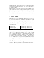
proof, try to set options, and after that try again. Bliksem can be called in one
of 4 following ways:
bliksem
bliksem
bliksem
bliksem
input
< input
input > output
< input > output
Input
Input
Input
Input
from
from
from
from
input, output
input, output
input, output
input, output
to
to
to
to
screen.
screen.
output.
output.
As can be seen from the table, Bliksem can read input from stdin, or from
a specified file. It always sends its output to stdout. Both stdin and stdout
can be redirected. Bliksem does not use stderr. It is also possible to type the
input directly, but this is impractical. On some systems it may be necessary to
type ./bliksem, instead of bliksem, when Bliksem is in the current directory.
We describe the input-format of Bliksem. The definition of the input syntax is
two-level. We first define a representation language which is able to represent
certain tree-like structures as strings of characters. After that we define additional typing rules that specify which trees are well-formed formulae, clauses,
or commands.
2.1
The Representation Language
All input to Bliksem is given in the representation language, independent on
whether it is a command, a formula or a clause.
2
Names
A sequence of one or more of the following characters is called name:
’a’..’z’, ’A’..’Z’, ’0’..’9’, ’_’, ’?’, ’$’, ’%’.
Whitespace
A sequence of one or more of the following characters is called white whitespace:
’\t’,
’\n’,
’ ’.
So possible characters in whitespace are the TAB-character, the end of line
character, and the space. Strings of the following form are called comment:
’/*’ ... ’*/’.
’#’ ... ’\n’.
In the first case there can be no earlier occurrence of */ . In the second case
there can be no earlier occurrence of \n .
For the sake of completeness we mention another way in which names can be
built. They can also be built using the double quotes ( " ). Between the quotes
there should be no end-of-line character, and no other double quote. Names of
this form should not be used in formulae. They have been included in the
representation language in order to make it possible to represent file names in
the representation language.
Using the names it is possible to recursively build up the expressions in the
representation language. There are functional expressions, lists, and expressios
built using certain built in syntactical operators.
Expressions of the Representation Language
The input of Bliksem consists of a sequence of expressions of the representation language, each of which is followed by a ( . ). Expressions are recursively
defined. Every name is an expression. If E1 , . . . , En , with n > 0 are expressions,
and f is a name, then
f ( E_1, ..., En )
is an expression. If E1 , . . . , En , with n > 0 are expression, then
{ E1,..., En }
is an expression. Finally expressions can be built up using predefined operators
from the following table:
3
Operator
Associativity
Priority
+, ^
*, /
+, -
prefix
rightassoc
leftassoc
leftassoc
140
130
120
110
=, ==>
nonassoc
100
==, !=, !==
<, >, <=, >=, >>, <<
>>=, <<=, >>==, <<==
:
nonassoc
nonassoc
nonassoc
nonassoc
100
100
100
100
!
&
|
<->
->
<>, []
[ a1, ..., an ]
< a1, ..., an >
prefix
leftassoc
leftassoc
leftassoc
rightassoc
prefix
prefix
prefix
80
70
60
50
10
10
10
10
||, &&, {}
constant
Most of the operators in the table have no fixed meaning. It is not possible
for the user to define operators. The reason for this is that with user defined
operators one needs the so called Prolog convention to resolve ambiguities:
In an expression of the form f(t1, ..., tn), no whitespace is allowed between the f, and the (.
The prolog convention is a source of syntax errors, and we feel that it is better
not have it. Instead there is a large set of predefined syntactical operators
without fixed meaning that can be freely used. However some of the operators
have an intended meaning when they are used in formulae, see the table in
Section 2.2.
In expressions of the form [ a1, ..., an ] Exp and < a1 ,..., an > Exp,
the ai should be names, and n > 0. In the expressions of the form [] Exp,
and <> Exp, there is no space allowed between the brackets. Similarly inside {}
no space is allowed.
4
Some of the operators do not exist internally, and they are replaced on reading
by other operators. These operators are in the following table:
operator
[ a1, ..., an ] Exp
< a1, ..., an > Exp
E1 != E2
E1 !== E2
is replaced by
[
<
!
!
a1 ]
a1 >
( E1
( E1
... [ an ] Exp
... < an > Exp
= E2 )
== E2 )
When an operator has a higher priority, it has a stronger binding strength.
When a conflict arises between two operators with the same priority, the associativity determines how it will be resolved. We give a list of examples of
expressions, for the intended meanings see Section 2.2
[ x ] x + 0 = x.
[ x, y ] x + succ( y ) = succ( x + y ).
[ x, y ] subset( x, y ) <-> [ z ] z : x -> x : y.
[ x, y ] ! subset( x, y ) <-> < z > z : x & ! x : y.
( ! [ x ] p(x) ) <-> < x > ! p(x).
a & b | c <-> ( a | c ) & ( b | c ).
Note that the representation language is too liberal:
[ a, b ] ( a -> b ) = ( ! a | b ).
[ a, b ] ( a & b ) = [ p ] ( a -> b -> p ) -> p.
[ a, b ] ( a | b ) = [ p ] ( a -> p ) -> ( b -> p ) -> p.
[ a ] ! a <-> [ p ] a -> p.
complexity( a -> b & c ) = 5.
( a -> b ) + ( b -> c ) = 2.
Sometimes the binding priorities can be counterintuitive:
# The K-rule is mostly written without parentheses.
( [] a -> b ) -> ( [] a ) -> [] b.
/* It is common to omit the parentheses.
*/
( [ x, y ] p ( x, y ) ) -> [ y, y, x ] p(x,y).
( [] a ) -> [] [] a.
# Mostly the -> binds stronger than the <->. Not in Bliksem.
5
! a | b <-> a -> b
2.2
/* means */ ( ! a | b <-> a ) -> b.
Well-Formed Formulae
The representation language allows representation of first order formulae, modal
formulae, and clauses. The following operators are used for this purpose. They
have fixed meanings.
! A
A & B
A | B
A -> B
A <-> B
<> A
[] A
< a1, ..., an > A
[ a1, ..., an ] A
||
&&
x : A
=
==>
¬A
A∧B
A∨B
A→B
A↔B
3A
2A
∃a1 · · · an A
∀a1 · · · an A
⊥
>
x∈A
=
⇒
The definitions of formulae and clauses are essentially recursive, but first-order
formulae and clauses need to satisfy some additional conditions. First the recursive types are defined, using capitals. After that we give the additional
conditions.
TERM
A name is a TERM. If t1, ..., tn, with n > 0 are TERMS, then
f(t1, ..., tn) and { t1, ..., tn } are TERMS. {} is a TERM. If t is a
TERM, then + t, - t are TERMS. If t1 and t2 are TERMS, then
t1 ^ t2, t1 * t2, t1 / t2, t1 + t2, t1 - t2
are TERMS.
ATOM
A name is an ATOM. If t1, ..., tn, with n > 0, are TERMS, then f(t1, ..., tn)
is an ATOM. If t1 and t2 are TERMS, then
t1 = t2, t1 ==> t2, t1 == t2, t1 !== t2, t1 : t2,
t1 < t2, t1 > t2, t1 <= t2, t1 >= t2,
t1 >> t2, t1 << t2, t1 >>= t2, t1 <<=, t1 >>== t2, t1 <<== t2
6
are ATOMS.
LITERAL
An ATOM is a LITERAL. If A is an ATOM, then ! A is a LITERAL.
FORMULA
An atom is a FORMULA. Both || and && are FORMULAS. If F is a FORMULA, then ! F is a FORMULA. If F1 and F2 are FORMULAS, then
F1 | F2, F1 & F2, F1 -> F2, F1 <-> F2
are FORMULAS. If a1, ..., an are names, and F is a FORMULA, then
[ a1, ..., an ] F, < a1, ..., an > F
are FORMULAS.
MODFORM
A name is a MODFORM. Both || and && are MODFORMS. If A is a MODFORM, then ! A, <> A, [] A are MODFORMS. If A1, A2 are MODFORMS,
then A1 | A2, A1 & A2, A1 -> A2, A1 <-> A2 are MODFORMS.
LITERALLIST
The empty list {} is a LITERALLIST. If all Li are LITERALS, and n > 0,
then { L1, ..., ln } is a LITERALLIST.
Observe that there is overlap between the recursive types. For example expression a & b is both a FORMULA and a MODFORM. Similarly expression
p(t1, ..., tn) is both a FORMULA, LITERAL, TERM, and ATOM.
Prolog Variable A name is a Prolog variable if its first character is a capital. This does not depend on the fact whether or not the name uses double
quotes (").
Formula
An FORMULA is a Formula if it does not contain a free Prolog variable that
is a TERM.
Modal Formula
A MODFORM is a modal formula if it does not contain a Prolog variable.
Clause
A LITERALLIST is a clause. In a clause of this form, Prolog variables are
treated as variables, when they occur on a position with type TERM.
A FORMULA is a clause on the condition that it does not contain
->, <->, < a1, ..., an > A,
7
and every ! occurs directly against an atom, i.e. in a LITERAL, and it does
not contain a free Prolog variable that is a TERM.
The following names are Prolog variables:
X, Y, Z, Abc, "A B C", "Buenos Aires".
Prolog variables are forbidden in formulae because their meaning is confusing.
In the clause { p(X), q(X) }, the Prolog variable X is a variable. In the clause
p(X) | q(X) it would be a constant, because free names in formulae are constants. Once Prolog variables are forbidden in formulae, they also have to be
forbidden in modal formulae. The modal formula [] A would be translated into
[x] R(w,x) -> x : A, which would have A as a free variable. The following
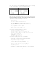
table contains a list of first order formula in Bliksem format, and their meanings.
First order Formulae and
[x,y] x + y = y + x.
[x,y,z] x < y -> y < z -> x < z.
[x,y] x : pow(y) <-> subset(x,y)
a -> ! a -> || .
a <-> b -> !a <-> !b
their meanings
∀xy(x + y = y + x).
∀xyz(x < y → (y < z → x < z)).
∀xy(x ∈ pow(y) ↔ subset(x, y)).
a(→ (¬a) → ⊥).
(a ↔ b) → ((¬a) ↔ (¬b))
The following clause set is not satisfiable:
{ ! nat(X), nat(s(X)) }.
{ nat(0) }.
{ ! nat( s(s(s(s(s(s(s(s(s(s(0)))))))))) ) }.
The following modal formulae are universally valid:
( <> a | b ) <-> ( <> a ) | <> b. # note the parentheses
( [] a & b ) <-> ( [] a ) & [] b.
The syntax is quite liberal, and it allows some pretty pervert expressions:
[
[
[
[
X ] ! X | X. # the quantified X does not bind the predicates X.
Y ] ! X | X. # is the same formula.
X ] X(X). # is well-formed.
A, B, C ] A | B -> ( A -> C ) -> ( B -> C ).
/* is well-formed, but does not have the usual meaning. */
{ X, ! X, X(X) }. # denotes the same clause as
{ X, ! X, X(Y) }. # It can resolve with
{ ! X(0) } # into
{ X, ! X }.
{ ! "[] <> A " ( "a & b" ) } /* and */
{ "[] <> A "("A & B"), "<> [] A "("A & B") }
/* resolve into */
{ "<> [] A "("a & b") }.
8
3
The Normal Form Transformation
4
The Calculus
5
User Options
In this section we discuss the user options that can be set. Since all input to
Bliksem is in the representation language, the user option settings also have to
be valid expressions of the representation language.
5.1
Output Format
Set( showgenerated, N ).
N should be 0 or 1. If N = 1, clauses are printed at the moment that they are
generated, before they are demodulated, or checked on redundancy. Default is
N = 0.
Set( showkept, N ).
N should be 0 or 1. If N = 1, clauses are printed at the moment that they are
kept, after they have been sorted. Default is N = 0.
Set( showselected, N ).
N should be 0 or 1. If N = 1, clauses are printed at the moment that they are
selected. If the clause can be simplified or if it is subsumed at the moment of
selection, it will be not printed. Default is N = 0.
Set( showdeleted, N ).
N should 0 or 1. If N = 1, clauses are printed when they are deleted by backward subsumption, or when they can be simplified into another clause. Default
is N = 0.
Set( showresimp, N ).
N should be 0 or 1. If N = 1, Bliksem tells when it is doing a resimplification.
Default is N = 1.
Set( showstatus, N ).
N should be between 0 and 10000000. Bliksem prints out a status report, each
time when approximately N clauses are kept. This is useful when all the other
printing options are switched of. If N < 10, no status reports are printed. Default is N = 2000.
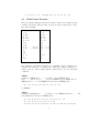
Set( prologoutput, N ).
N should be between 0 and 3. If N = 0, the output is in Bliksem-syntax. If
N = 1, 2, 3, the output is in Prolog-syntax. The difference is in the treatment
of variables. If N = 1, variables have form X,Y,Z,T,U,W,V0,V1,... Because
9
the handling of names starting with a capital is problematic in Prolog, there are
also the following options: If N = 2, variables have form vvvv_(i) If N = 3,
variables have form vvvv_i.
Set( totalproof, N ).
N should be 0 or 1. If N = 1, Bliksem outputs the proof with explicit substitutions and permutations.
5.2
Derivation Rules
Set( useres, N).
N should be 0 or 1. If N = 1, then (always ordered) binary resolution is used.
Default is N = 0.
Set( useparamod, N).
N should be 0 or 1. If N = 1, then (ordered) paramodulation is used. Default
is N = 0.
Set( useeqrefl, N).
N should be 0 or 1. If N = 1, then the unordered equality reflexivity rule is
used. Default is N = 0.
Set( useordeqrefl, N).
N should be 0 or 1. If N = 1, then the ordered equality reflexivity rule is used.
Default is N = 0.
Set( useeqfact, N).
N should be 0 or 1. If N = 1, then the (ordered) equality factoring rule is used.
Default is N = 0.
Set( usefactor, N).
N should be 0 or 1. If N = 1, then unordered factoring is used. Default is N = 0.
Set( useordfactor, N).
N should be 0 or 1. If N = 1, then ordered factoring is used. Default is N = 0.
Set( usesimpdemod, N).
N should be ≥ 0. Sets the maximal length that a clause can have in order
to be a demodulator. Setting N ≤ 0, means that there is no demodulation.
Demodulation is attempted when a clause is generated, when it is selected,
and when it is resimplified. Setting N large can have the consequence that a
very large discrimination tree of useless demodulators is built. Default is N = 0.
Set( usesimpres, N).
N should be ≥ 0. Sets the maximal length that a clause can have in order to be a
resolution simplifier. Setting N ≤ 0 means that there is no resolution simplifica10
tion. Setting N large can have the consequence that a very large discrimination
tree of useless simplifiers is built. Resolution simplification is attempted when a
clause is generated, when it is selected, and when it is resimplified. The default
is N = 0.
Set( resimpinuse, N).
N should be between 10 and 1000000. Each time when approximately N clauses
have been generated, Bliksem will do a resimplification of the clauses in inuse.
This means that they are processed as if they have just been generated. They
are checked for subsumption, and possibly demodulated or simplified by resolution. Default is N = 2000.
Set( resimpclauses, N).
N should be between 100 and 10000000. Each time when approximately N
clauses have been generated, Bliksem will do a resimplification of the clauses in
clauses. This means that they are processed as if they have just been generated.
They are checked for subsumption, and possibly demodulated or simplified by
resolution. The default value is N = 20000.
Set( substype, S).
Sets the type of subsumption. S can have the following 3 values: standard:
This selects standard subsumption. standard is the default value. snl1: This
selects weak subsumption of type SNL1. eqrewr: This makes subsumption take
into account the commutativity of = , and the fact that = and ==> mean
the same.
Set( selectoldest, N).
Bliksem selects N − 1 times the lightest clause, and then 1 time the oldest. This
introduces some fairness into the selection process. If N = 0, Bliksem always
selects the oldest clause. The default value is N = 10.
5.3
Setting the Weights
Weights are used in Bliksem for selection clauses. Bliksem selects most of the
time, (dependent on the value selectoldest), the lightest clause. The weight
of a clause is computed by adding the weights of the occurrences of the operators in the clause. The weights of the operators can be set, using Set weight.
A variable always has weight 1. Currently there is no way of having more sophisticated weight functions, for example giving different weights to different
arguments of a certain operator. A weight assignment has the following form:
Set weight( f (t1 , . . . , ta ), N ).
This assigns a weight of N to the operator f, when it occurs with arity a. The
11
arguments ti are used only for determining the arity, so what the ti actually
are, does not matter. It is possible to assign weights to the built in operators.
By default, the weight of each operator is set to 1. Possible weight assignments
are:
Set_weight(
Set_weight(
Set_weight(
Set_weight(
p(X,Y), 400 )).
1 + 1 = 2, 10 ).
! x, 0 ).
a & b, 5 ).
#
#
#
#
assigns weight 400 to p with arity 2.
Assigns a weight of 10 to equality.
Assign a weight of 0, to negation.
Possible, but useless.
5.4
Setting the Order
5.5
Complexity Restrictions
Set( maxweight, N).
Set the maximal weight that a kept clause can have. Default is N = 30000.
Set( maxdepth, N).
Set the maximal depth that a kept clause can have. Default is N = 30000.
Set( maxlength, N).
Set the maximal number of literals that a kept clause can have. Default is
N = 45.
Set( maxnrvars, N).
Set the maximal number of distinct variables that a kept clause can have. Default is N = 95.
Set( maxselected, N).
Set the maximal number of clauses that can be selected. When N is exceeded,
the search process will stop. What happens next depends on the other options.
Default is N = 10000000.
Set( maxkept, N).
Set the maximal number of clauses that can be kept. When N is exceeded the
search process will stop. What happens next depends on the other options.
Default is N = 10000000.
Set( excuselevel, N).
Clauses with a level ≤ N are allowed to violate the complexity restrictions
maxweight, maxdepth, maxlength and maxnrvars. Initial clauses have
level 0. Default is N = 0.
Set( increasemaxweight, N).
If N > 0, then after a failed proof attempt, maxweight is increased by N, and
another attempt is made. Default is N = 0.
12
6
Formatted Proofs
7
Example Inputs
7.1
Composition of Orders
7.2
Rubik’s Cube
7.3
Commutativity of Addition
13