Download CEM_SWAN_manual

 {
User Guide to Coupling SWAN
and CEM Table of Contents INTRODUCTION Basic model structure 3 3 Pre-­simulation set-­up Directory Structure Necessary files and scripts 7 7 7  {In your home directory}  {In your working directory}  {In your local directory} 8 8 9 10 Parameters to adjust and know before starting your simulation Making your bathymetry, setting up your computational CEM domain, and dealing with periodic boundary conditions 13 Model steps and main function calls as executed by the RUN file Step 1: FindWaveAngle Step 2: Run SWAN coarse grid Step 3: Run SWAN nested grid Step 4: Run CEM Step 5: Save files to output folder 17 17 17 18 18 19 Post-­processing 20 Known issues and limitations 20 Step-­by-­step instructions using the sample files Part 1: Setting up the directory structure and uploading necessary files Part 2: Compiling the ‘.c’ files to make executables Part 3: Submitting your job Part 4: Using Matlab to view the model output 22 22 22 23 24 References 26 Appendix 27 2 INTRODUCTION The Coastline Evolution Model (CEM) simulates large-­‐scale coastline behavior caused by gradients in alongshore sediment flux (Ashton et al., 2001; Ashton and Murray, 2006a, 2006b). The wave climate, or the angle and direction of incoming waves relative to the local coastline orientation, is the forcing mechanism and determines the resultant long-­‐term coastline morphology (i.e., capes, spits, migrating sandwaves). Operating alone, CEM transforms waves in the most basic way by assuming shore-­‐parallel bathymetry contours that extend seaward only to the depth of the shoreface (10-­‐20 m). This simplification inherently excludes alongshore wave energy convergence/divergence, wave transformation over the shelf, and coastlines where bathymetry is complex (e.g. nearshore or cape-­‐
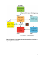
associated shoals; van den Berg et al., 2012; Kaergaard and Fredsoe, 2013a, 2013b, 2013c). By replacing CEM’s basic wave shoaling routine with a more complex spectral wave transformation model (Simulating WAves Nearshore, or SWAN; Booij et al., 1999; Ris et al., 1999), CEM can simulate a broader array of coastline behaviors, especially those influenced by nearshore shoals or irregular bathymetry. This manual details how the coupling between CEM and SWAN was accomplished, and how to couple CEM and SWAN on the UF High Performance Computing Cluster. Basic model structure Before proceeding, you need a scripting-­oriented text editor. For Mac, Xcode (free; version 5, or greater) is highly recommended. Aquamacs or TextWrangler will also work. CEM and SWAN are two separate, standalone models, written in C and Fortran, respectively. Because they ‘speak’ different languages, CEM and SWAN do not communicate directly with each other. Instead, the models communicate through a 3 UNIX shell script (called a ‘RUN file’). The RUN file acts as a translator between the models by executing SWAN and CEM sequentially and mediating the exchange of information (input-­‐output) between SWAN and CEM. The RUN file can be set to perform as many model iterations as necessary. To couple SWAN and CEM, no changes have been made to the SWAN program; it is run as it would without CEM. There are, however, some critical SWAN parameters that must be set correctly to ensure successful input-­‐output between SWAN and CEM (see the ‘Pre-­‐simulation set-­‐up’ section below). Several major changes have been made to CEM in order to couple it with SWAN. All changes are flagged with the hashtag #SWAN within the CEM_SWAN.c file so they are easily searchable. The most noteworthy changes to CEM are: 
The main time loop that sets the number of model iterations in a given simulation has been made external to CEM; it is now implemented in the RUN file. CEM is set to run for only ONE time step each time it is called by the RUN file, and it loads the shoreline position from the previous model iteration to use as initial conditions. 
The basic wave shoaling routine no longer exists within CEM, as it is replaced by SWAN. 
The ‘FindWaveAngle’ routine that selects a random deep-­‐water wave angle before each model iteration has been made external to CEM. It is now a stand-­‐alone executable program called by the RUN file because it must inform SWAN, rather than CEM, of wave boundary conditions. 
A new function called “LoadSWAN” was added that inputs SWAN’s output grids (wave height, angle) as well as bathymetry. 4 
A new function called “ParseSWAN” was added that finds breaking wave height and angle from the SWAN grids loaded in the function “LoadSWAN”. For each model shoreline cell, the routine searches seaward until a breaking wave threshold (wave height divided by water depth) is found. Then the wave height and angle are stored and used later to calculate alongshore sediment flux with the CERC equation. 
A new function called “SaveSWANToFile” was added. This function completes two key tasks after CEM has calculated alongshore sediment flux gradients and updated shoreline position. First, using the updated shoreline position, it linearly interpolates the shoreface bathymetry seaward from each model shoreline cell using the user-­‐inputted shoreface depth and slope. Then, using the bathymetry from the earlier SWAN simulation, the new shoreface bathymetry is merged with the shelf bathymetry. Second, the updated shoreface/shelf bathymetry grid is written to file so that SWAN can input it during the next model iteration to calculate a new set of wave heights and angles. 
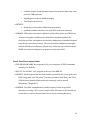
A new function called “ConvertAngle” was added that converts the angle convention used by SWAN (azimuth, 0° or 360° is shore-­‐normal) to the convention used by CEM (-­‐90° ≤ wave angle ≤ 90°, where negative angles come from the left and positive from the right). The SWAN/CEM coupled model is executed using the RUN file that is submitted as a job to the HPC cluster. Figure 1 is a flow chart showing the order of operations dictated by the RUN file. The following sections explain each colored boxes in Figure 1 in detail, including the inputs and outputs in each step. 5 Figure 1. Flow chart of the coupled SWAN and CEM model. Each colored box, or step, is explained in the manual. 6 Pre-­‐simulation set-­‐up Setting up your CEM/SWAN simulation is generally the same as setting up a nested SWAN run, with a few added steps (this manual assumes the reader knows how to set up a SWAN run on the HPC cluster, and has a basic understanding of the shell script). Directory Structure On the HPC cluster, the RUN file will be stored in your Home directory (/home/username) from where it will be submitted as a job. Within your home directory, the model saves files as the model runs in an ‘output’ subdirectory (/home/username/output). The computation does not take place in your home directory. This happens in your ‘working’ directory on the HPC’s scratch drive (/scratch/lfs/username). To summarize: the RUN file is stored and submitted as a job from your home directory; the RUN file sequentially calls executables (CEM, SWAN, etc.) located in your working directory; and as the model runs, files you wish to save are moved automatically to your output directory. On your local hard drive, you will need a directory to store your output (downloaded from the HPC) where Matlab scripts, described below, are executed to parse and display model output. Necessary files and scripts Before running SWAN+CEM, the following files must be placed in the correct directories and must be named as specified below, unless indicated otherwise. 7 Each file is explained in detail below. (Note that you do not need to put any files in your output directory.)  {In your home directory}  RUN file – can be named whatever you like.  SWAN4091 – the folder containing the SWAN program and executable.  {In your working directory} Files that are updated/changed during the model run:  Depth.bot – bathymetry input file for nested SWAN run that is updated each timestep by CEM as the shoreline position changes. Values below sea level are positive, and subaerial values are negative.  0 – initial shoreline conditions for CEM. The name corresponds to the timestep, and each time the shoreline is updated CEM exports a new shoreline file named after the current timestep. Files that are NOT updated/changed during the model run:  Depth_main.bot – bathymetry for the coarse-­‐grid (or main) SWAN run that supplies boundary conditions for the nested run.  CEM_SWAN.c – CEM model that must be compiled to an executable file. 8  FindWaveAngle.c – Generates a new, random deep-­‐water wave angle from a probability distribution function each time step. Must be compiled to an executable file.  finegrid.swn – SWAN file corresponding to your nested SWAN run.  In addition to the above files, you must have 181 main SWAN files in your working directory. Each file has a unique integer deep-­‐water wave angle as a boundary condition, and controls the coarse-­‐grid SWAN runs that supply boundary conditions for the nested runs. They must be named sequentially 1000.swn – 1090.swn and 1270.swn – 1360.swn. The last 3 numbers in the file names correspond to the deep-­‐water wave angle in azimuthal degrees relative to the coast that is indicated within the file. The angle is selected each time step by the ‘FindWaveAngle’ function. For example, if the FindWaveAngle function selects a wave angle of 43 degrees, the SWAN file 1043.swn will be called and will execute a coarse-­‐grid SWAN run based on that angle.  {In your local directory}  makeinitconds.m: This script will create the initial shoreline conditions file called “0” (see above) from your nested SWAN bathymetry grid.  postprocess.m: Main script for viewing and plotting model output. Execute the script on your local directory containing model output, and it will load the whatever output you tell it to (wave height, wave angle, bathymetry, etc.).  animateoutput.m: Animates output files through time and compiles them into movie (.avi) files. 9  sort_nat.m: Sorting routine; must be present with your model output (i.e. in the same folder) when running postprocess.m. Parameters to adjust and know before starting your simulation Below is a list of all parameters that need to set before starting your model run. Use the CEM/SWAN Reference Guide to see where these variables are located within each file. { IN CEM_swan.c } •
Cell size: This must be set exactly the same as the cell size in the nested SWAN run. Generally, CEM works best when cell size is 100 m or greater, so use that as a guide to set your nest grid cell size. In order to spatially resolve the wave breaking threshold (see below), a cell size less than 500 m for your simulation is suggested. •
Cross-­shore domain size: Called ‘Xmax’ in CEM. Should be exactly the same as the cross-­‐shore extent of your nest SWAN grid. NOTE: when entering grid dimensions to your .swn files, SWAN requires them to be number of meshes rather than number of grid cells. The number of meshes is the number of grid cells minus one. So, if your bathymetry grid size is 100 cross-­‐shore cells by 100 alongshore cells, in CEM you would enter 100 x 100; however, in the .swn files, you would enter 99 x 99. •
Alongshore domain size: Called ‘Ymax’ in CEM. Should be 0.5 of the alongshore extent of your nest SWAN grid. NOTE: when entering grid dimensions to your .swn files, SWAN requires them to be number of meshes rather than number of grid cells. The number of meshes is the number of grid cells minus one. So, if your bathymetry grid size is 100 cross-­‐shore cells by 100 alongshore cells, in CEM you would enter 100 x 100; however, in the .swn files, you would enter 99 x 99. 10 •
Shoreface depth: Called ‘DepthShoreface’ in CEM. Typical values range from 10-­‐20 m. It is the depth over which sediment is evenly distributed as it is transported alongshore. If the shoreline moves landward, a ravinement surface is left behind corresponding to the shoreface depth (see Ashton and Murray, 2006a). If the shoreface and shelf bathymetry are not merging smoothly in the SaveSWANToFile function in CEM, shoreface depth can be adjusted to improve the fit. Note, however, that adjusting the shoreface depth affects the timescales for shoreline adjustment (Ashton and Murray, 2006a). •
Shoreface slope: Called ‘ShorefaceSlope’ in CEM. Typical values range from 0.005 to 0.05. If the shoreface and shelf bathymetry are not merging smoothly in the SaveSWANToFile function in CEM, shoreface slope can be adjusted to improve the fit. •
Wave breaking threshold: Called ‘WaveBreakDepth’ in CEM. Typical values range from 0.8 to 0.3. The lower the number, the farther offshore CEM will look to find a “breaking” wave. The SWAN-­‐generated wave heights and angles are most accurate at least a couple cells seaward of the shoreline cell, so using a lower number works best (0.3 – 0.5). See List and Ashton (2007) for a discussion of this. In order to spatially resolve the wave breaking threshold, a cell size less than 500 m for your simulation is suggested. If the cell size is too big, the wave breaking threshold will be exceeded for every nearshore cell and faulty wave characteristics will be retrieved. { IN coarse-­‐grid .swn files } •
Wave height: Wave height is specified within the .swn files that control your coarse grid SWAN runs. It must be the same in all 181 files. Rather than edit each file individually when wave height and/or period need to be changed, use the current version of Xcode (5.0.1) to find and replace text within your workspace (i.e., it will change the wave conditions for all 181 files at once; see specific instructions below). •
Wave period: Wave period is specified within the .swn files that control your coarse grid SWAN runs. It must be the same in all 181 files. 11 •
Cell size of coarse SWAN grid: Cell size can be whatever you wish. The cell size of the nested grid, however, must match the cell size of CEM. •
Domain size coarse SWAN grid: Size can be whatever you wish; although it is beneficial for the coarse-­‐grid alongshore length to be at least 5 times the length of the nested domain (with the nest in the center) to avoid edge/boundary effects. In the cross-­‐shore direction, the grid should extend to true deep water (depth > 0.5*wavelength). •
Where to apply boundary conditions (wave height, angle, period): Wave conditions are applied by the user at the top (or seaward) boundary of the coarse grid only. The nested SWAN run automatically receives boundary conditions from the coarse-­‐grid SWAN run. { IN FindWaveAngle.c } •
Wave climate asymmetry: Assigned using the variable ‘asym’. It must range from 0 – 1, with a value of 0.5 meaning an equal number of waves come from the left and right directions. Wave asymmetry is a property that can be found for a given coastline using wave buoy data (see Ashton and Murray, 2006a, 2006b). •
Proportion of high-­angle waves: Assigned using the variable ‘highness’. It must range from 0 – 1, with a value of 0 meaning all deep-­‐water waves are <45 degrees (low-­‐angle). This is a property that can be found for a given coastline using wave buoy data (see Ashton and Murray, 2006a, 2006b). { IN nest-­‐grid .swn file } •
Cell size of nested SWAN grid: This must be set exactly the same as the cell size in CEM. Generally, CEM works best when cell size is 100 m or greater, so use that as a guide to set your minimum nest grid cell size. To set the maximum cell size, consider that the wave breaking threshold (wave height divided by depth) must be spatially resolved. Because of this, a cell size less than 500 m is optimal. •
Cross-­shore domain size: Must be the same as in CEM, or equal to Xmax. 12 •
Alongshore domain size: Must be equal to 2*Ymax and set up according to Figure 2 and the periodic boundary conditions (see following section). { IN Run file } •
Time steps: Stored in variable ‘t’, this controls the number of times the main time loop iterates. •
Internal time steps: To speed up the simulation, the same SWAN output can be used for multiple CEM iterations. By doing this, SWAN does not regenerate a wave field every time step. The number of times to internally loop CEM with the same wave conditions is stored in the variable ‘ti’. The underlying assumption is that shoreline position does not change appreciably over one time step, so the same waves can be used multiple times; this assumption breaks down when ti ~> 5. If you do not want to engage the internal loop (i.e., you want SWAN to generate new waves every time step), set ti = 1. •
Working directory name and location: Make sure the working directory location is correct. Your working directory name must be the same as your output directory name. •
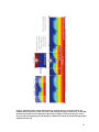
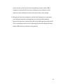
How many files you wish to save during the simulation: Use the variable ‘cull’ for this. For example, if you want to save model output every 100 time steps, set cull = 100. Making your bathymetry, setting up your computational CEM domain, and dealing with periodic boundary conditions Orienting your SWAN and CEM computational domains appropriately is the most critical step in coupling the models. Your bathymetry and shoreline domains must be set up as in Figure 2. Incorrect grid sizes, locations, and cell sizes are the most common causes of model crashes or faults. All computational domains for SWAN and CEM (bathymetry for SWAN, shoreline position for CEM) must be oriented with the offshore direction facing up or north. 13 Figure 2 shows how the bathymetry must be set up for the SWAN runs, and how it relates to the CEM computational domain. Variables listed above (e.g., Ymax, Xmax) are also shown in Figure 2. SWAN bathymetry can be set up as it would for any usual nested SWAN run, but you must make certain that the nested grid is located correctly within the coordinate space of the coarse/main grid, and the cell size of the nested grid is the same as the cell size of the CEM domain. The boundary conditions in CEM are periodic, meaning that 1) sediment is conserved, 2) sediment that fluxes out of the right boundary comes back through the left boundary and vice versa, and 3) the shoreline domain is therefore effectively repeated to infinity alongshore. To impose periodic boundary conditions, CEM’s main computational domain (defined by Ymax and Xmax) is split down the middle. The right half is placed adjacent to the left boundary, and the left half is placed adjacent to the right boundary (see Figure 2). Thus CEM effectively operates on an alongshore distance of 2*Ymax. The nested SWAN grid over which the wave field is computed must be set up the same way, with a central domain defined by Ymax and Xmax that is split into two halves that are placed on either boundary. This ensures that CEM will have a ‘smooth’ and continuous wave field to read when it applies periodic boundary conditions. The practical effects on SWAN of imposing periodic boundary conditions in CEM are summarized as follows: → The nested bathymetry grid must be of alongshore size 2*Ymax and cross-­‐shore size Xmax. The central grid that corresponds to the CEM domain is of size Ymax by Xmax and is defined on the left by Ymax/2 and on the right by (3*Ymax)/2 (see Figure 2). → The cross-­‐shore shoreline position on the left and right edges of the central domain (defined on the left by Ymax/2 and on the right by (3*Ymax)/2) must be equal. This applies to both SWAN and CEM (see below). Otherwise there will be a discontinuity when CEM applies periodic boundary conditions. 14 Wave direction or angle conventions are different between SWAN and CEM: in SWAN, wave direction is azimuthal where 0°/360° is shore-­‐normal, 270° is directed left and 90° is directed right; in CEM, 0° is also shore-­‐normal, but -­‐90° is directed left and 90° is directed right (see Figure 2). Once your SWAN bathymetry grids are complete, the initial conditions for CEM (the file is called “0” in the file list above) can be extracted from the nest grid. Cells in the CEM domain all contain values between, or equal to, 0 and 1 that specify how ‘full’ the cell is with sediment (Ashton and Murray, 2006a). Thus cells can either be land (cell is full, or equal to 1), water (cell is empty, or equal to zero), or shoreline (cell has a fractional value between zero and one). Thus, in the nest bathymetry grid, values greater than and equal to sea level (zero elevation) are assigned a value of 1, values less than sea level are assigned a value of zero, and the seaward-­‐most cells greater than or equal to sea level are assigned a fractional number (e.g., 0.5). These fractional cells are the shoreline. A Matlab script called makeinitconds.m is supplied that will convert your nest bathymetry grid to CEM initial conditions and produce a text file called “0”. 15 Figure 2. Schematic of the computational domains, and how they are spatially related. The variables Xmax and Ymax are the cross-­shore and alongshore lengths, respectively, of the CEM domain. Conventions used to define wave direction (or angle) are shown by the gray circles. The procedure for imposing periodic boundary conditions is shown on the bottom right (and is explained in the text). 16 Model steps and main function calls as executed by the RUN file Each step below is labeled and annotated within the RUN file. Reading this section with the RUN file at hand is recommended. Step 1: FindWaveAngle → FILE/PROGRAM NAME: FindWaveAngle, an executable file created by compiling FindWaveAngle.c → INPUTS: None → OUTPUTS: •
‘AngleDegrees.txt’, a text file containing a deep-­‐water wave angle in azimuthal degrees (to be used by SWAN and CEM) → PURPOSE: Extracted from the original CEM, this stand-­‐alone function creates a PDF of waves based on wave asymmetry (A) and 'highness' (U, proportion of waves that are >~42). From this PDF, CEM picks 'randomly' each model day a deep-­‐water wave to drive the daily model simulation. The PDF function is made external to CEM because SWAN needs to know the deep-­‐water wave angle to generate a wave field before CEM is called. The output, a text file, contains the generated wave angle. The RUN file reads the text file and the wave angle is assigned to a variable called “temp”. The variable “temp” is then used to call the corresponding SWAN coarse-­‐grid file. Step 2: Run SWAN coarse grid → FILE/PROGRAM NAME: “temp”.swn → INPUTS: •
Depth_main.bot → OUTPUTS: 17 •
Boundary conditions for nested SWAN run. This will also output grid plots of wave height and angle for the coarse grid, if you like. This is useful for debugging. → PURPOSE: To generate boundary conditions for the nested SWAN run. Step 3: Run SWAN nested grid → FILE/PROGRAM NAME: finegrid.swn → INPUTS: •
Boundary conditions from coarse-­‐grid SWAN run •
Depth.bot (from CEM) → OUTPUTS: •
“Hsig”, a text file containing a Ymax by Xmax matrix of significant wave heights (to be used by CEM) •
“Dir”, a text file containing a Ymax by Xmax matrix of wave directions (to be used by CEM) → PURPOSE: The nested SWAN run creates the nearshore wave conditions, stored in the “Hsig” and “Dir” text files, used to calculate alongshore sediment transport in CEM. If results from a non-­‐nested SWAN run are used as input for CEM (i.e., wave conditions are generated from a single SWAN run), then the calculated wave field will have edge effects (see SWAN user manual) and will not be usable by CEM. Step 4: Run CEM → FILE/PROGRAM NAME: cem, and executable file created by compiling CEM_SWAN.c. → INPUTS: •
“Hsig” (from SWAN) •
“Dir” (from SWAN) •
Depth.bot (from previous CEM iteration) 18 •
coastline domain (with the same name as the previous time step, from previous CEM iteration) •
AngleDegrees.txt (from FindWaveAngle) •
TimeStep.txt (see below) → OUTPUTS: •
Depth.bot (to be used by SWAN in next iteration) •
updated coastline domain (to be used CEM in the next iteration) → PURPOSE: CEM reads in the wave conditions produced by the nested SWAN run, calculates alongshore sediment flux, distributes sediment, updates the shoreline position, and updates the shoreface bathymetry (extended seaward from the new shoreline position). The new shoreface bathymetry is merged with the SWAN nest bathymetry (Depth.bot), and in the next model iteration SWAN uses the new bathymetry to generate a new wave field. Step 5: Save files to output folder → FILE/PROGRAM NAME: No program or file, just a sequence of UNIX commands issued by the RUN file → INPUTS: The variable “cull” assigned at the top of the RUN file → OUTPUTS: Model outputs that are moved and saved include the coarse grid wave field (“Hsig_main” and “Dir_main”), the nest grid wave field(“Hsig” and “Dir”), CEM shoreline domain (named after the timestep), and the nested bathymetry (“Depth.bot”). → PURPOSE: The UNIX commands move model outputs/results at specified intervals (set using “cull”) to your output folder. Files that are not moved are overwritten to reduce the size (and clutter) in your working directory. 19 Post-­‐processing After your model run is complete, download your output to a local directory. Executing the Matlab script postprocess.m will load the saved model output (from your output folder) into Matlab for viewing, plotting, etc. The file is annotated thoroughly. The postprocess.m script calls a second script (animateoutput.m) that will 1) animate your loaded output files and 2) save them to a movie (.avi) file. In order to run postprocess.m and animateoutput.m, you must have the complementary Matlab script called sort_nat.m in your output directory. Postprocess.m calls sort_nat.m (you do not need to manually execute sort_nat.m or alter it in any way – it just needs to be present in your folder) to efficiently sort the output data before loading into Matlab. To understand how they work, these Matlab scripts are included with sample model output. Known issues and limitations 1) Running the model takes a long time. Using the variable ti in the RUN file, which uses the same SWAN output for multiple CEM iterations, can speed up the process significantly. However, it can still take several days to complete a simulation. There are probably several other ways, unexplored here, to speed up the simulations. 2) Currently the model can deal only with low-­‐curvature shorelines. This means no spits, or overhanging/recurving capes, or any shoreline that has multiple cross-­‐shore shoreline coordinates for a given alongshore coordinate. The 20 reason for this is that the shoreface interpolation routine within CEM is designed to interpolate the shoreface bathymetry very simply. It can be updated to deal with high-­‐curvature shorelines fairly easily, though. 3) Merging the shoreface bathymetry and the shelf bathymetry is sometimes not completed smoothly, meaning there is an elevation discontinuity between the shoreface and shelf that affects the SWAN-­‐generated wave field. This is something to watch out for. Adjusting the shoreface depth and slope within CEM can help troubleshoot the problem. 21 Step-­‐by-­‐step instructions using the sample files Part 1: Setting up the directory structure and uploading necessary files 1) Open FileZilla, CyberDuck, or other FTP program. Log in to your HPC account using SSH file transfer protocol and entering the address submit.hpc.ufl.edu. 2) Use the FTP program to upload the folder SWAN4091 to your home directory (/home/username). 3) Use the FTP program to upload the RUN file (‘RUN_swan_CEM’) to your home directory. 4) In your home directory (/home/username), create a directory called ‘output’. 5) Within the new ‘output’ directory, create a subdirectory named ‘testrun’. This is where the ‘testrun’ model output will be stored. 6) Now, navigate to your scratch directory: /scratch/lfs/username 7) Create a working directory there called ‘testrun’. This directory must have the same name as your ‘testrun’ output directory. 8) Using the FTP program, put the required files in your working directory: finegrid.swn, 0, Depth.bot, Depth_main.bot, FindWaveAngle.c, CEM_swan.c, and the 181 .swn files that control the coarse-­grid SWAN runs. Part 2: Compiling the ‘.c’ files to make executables 9) Open a terminal window. Log in to your HPC account by typing ssh submit.hpc.ufl.edu You will be prompted for your user name and password. 10) Navigate to your working directory: 22 cd /scratch/lfs/username/workingdirectory 11) Now you must compile the FindWaveAngle.c and CEM_swan.c files. For the FindWaveAngle.c file, enter the command: gcc –o FindWaveAngle FindWaveAngle.c –lm ‘gcc’ calls the compiler, ‘-­‐o’ is an option that allows you to specify the name of the executable that is generated by the compiler, ‘FindWaveAngle’ is the name of the executable (that is called by the RUN file), ‘FindWaveAngle.c’ is the program to be compiled, and ‘-­‐lm’ tells the compiler to add the necessary math libraries. Note that you must name the executable ‘FindWaveAngle’ because it is called by the RUN file using the same name. After you compile FindWaveAngle.c, the executable file will appear in your working directory. Double-­‐check: make sure the executable is called ‘FindWaveAngle’! Do the same thing for the CEM_swan.c file: gcc –o cem CEM_swan.c –lm This compiles the CEM, and the executable must be named ‘cem’ so that it can be called correctly by the RUN file. After you compile, the executable file will appear in your working directory. Check that it is called ‘cem’, all in lower-­‐case letters. Part 3: Submitting your job 12) In your terminal window, navigate to your home directory: cd /home/username 23 13) Before submitting your job, you must convert the RUN file to UNIX format. Type the command dos2unix RUN_file where ‘RUN_file’ is the name of your Run file, whatever that may be. 14) Now you are ready to submit your job by entering qsub RUN_file where ‘RUN_file’ is the given name of your RUN file. While your job is running, you can check its status by typing qstat –u username or delete your job by typing qdel jobID The ‘jobID’ is shown when you submit your job and can be found by using the qstat command. As your job runs, files will accumulate in your output directory. Part 4: Using Matlab to view the model output 15) Open Matlab. Set your Matlab working directory to your output directory, and make sure that directory has the sort_nat.m script in it. 16) Using the FTP program, download your model output to a local directory. 24 17) Open postprocess.m and make sure that the variables Ymax, Xmax, and cell size are set the same as in CEM. 18) Run postprocess.m. It will load all of your model output, and animateoutput.m will show you a movie. 25 References Ashton, A., A.B. Murray, and O. Arnoult (2001), Formation of coastline features by large-­‐scale instabilities induced by high-­‐angle waves, Nature, 414, 296-­‐300. Ashton, A. D., and A. B. Murray (2006), High-­‐angle wave instability and emergent shoreline shapes: 1. Modeling of sand waves, flying spits, and capes, J. Geophys. Res., 111, F04011, doi:10.1029/2005JF000422. Ashton, A. D., and A. B. Murray (2006), High-­‐angle wave instability and emergent shoreline shapes: 2. Wave climate analysis and comparisons to nature, J. Geophys. Res., 111, F04012, doi:10.1029/2005JF000423. Kaergaard, K. and J. Fredsoe (2013a), Numerical modeling of shoreline undulations Part 1: Constant wave climate, Coastal Engineering, 75, 64-­‐76. Kaergaard, K. and J. Fredsoe (2013b), Numerical modeling of shoreline undulations Part 2: Varying wave climate and comparison to observations, Coastal Engineering, 75, 77-­‐90. Kaergaard, K. and J. Fredsoe (2013c), A numerical shoreline model for shorelines with large curvature, Coastal Engineering, 74, 19-­‐32. van den Berg N., A. Falqués, and F. Ribas (2012), Modeling large scale shoreline sand waves under oblique wave incidence, J. Geophys. Res., 117, F03019, doi:10.1029/2011JF002177. 26 Appendix Below are commented copies of the files needed to run the SWAN/CEM model. They are intended as a reference that is complementary to the manual so that the user can see where the parameters and variables discussed in the manual are actually located in each model file. 27 finegrid.swn
!
Run ID Number: 20130222cpcnv1
!
Run Clock: 22-Feb-2013 13:55:33
!
!
SET LEVEL=0 NAUTical
MODE STATIONARY TWODimensional
COORDinates CARTesian
CGRID REGular 70080 0 0 70080 32640 219 102 CIRCLE 36 0.05 1
INPgrid BOTtom REGular 70080 0 0 219 102 320 320 EXC -99999
READinp BOTtom 1 'Depth.bot' 3 0 FREE
BOUNd SHAPespec JONswap 3.3 PEAK DSPR DEGR
BOUNdnest1 NEST 'cem_f' CLOSed
OFF QUAD
OFF BREAKING
GROUP 'compgrid' SUBGRID 0 219 0 102
QUANTITY HSIGN DIR excv=-5
OUTPUT OPTIONS BLOCK ndec=2 len=220
BLOCK 'compgrid' NOHEADER 'Hsig' HSIGN
BLOCK 'compgrid' NOHEADER 'Dir' DIR
COMPUTE
STOP 1009.swn
!
Run Clock: 22-Feb-2013 13:55:33
!
conditions: 1 m, 8 s, 0 deg, (10 deg spread)
!
!
SET LEVEL=0 NAUTical
MODE STATIONARY TWODimensional
COORDinates CARTesian
CGRID REGular 0 0 0 210240 65280 219 68 CIRCLE 36 0.05 1
INPgrid BOTtom REGular 0 0 0 219 68 960 960 EXC -99999
READinp BOTtom 1 'Depth_main.bot' 3 0 FREE
BOUNd SHAPespec JONswap 3.3 PEAK DSPR DEGR
BOUNdspec SEG IJ 0 68 219 68 CONSTANT PAR 2 10 9 10
OFF QUAD
OFF BREAKING
GROUP 'compgrid' SUBGRID 0 219 0 68
NGRID 'cem_s' 70080 0 0 70080 32640 219 102
QUANTITY HSIGN DIR excv=-5
OUTPUT OPTIONS BLOCK ndec=2 len=220
BLOCK 'compgrid' NOHEADER 'Hsig_main' HSIGN
BLOCK 'compgrid' NOHEADER 'Dir_main' DIR
NESTout 'cem_s' 'cem_f'
COMPUTE
STOP
cem_SWAN.c
/* CAPERIFFIC */
/* PWL's changes to this program for SWAN integration are initialed PWL with the date
/* and a searchable tag: #SWAN */
/* ----------------------------*/
#include
#include
#include
#include
#include
#include
<stdlib.h>
<stdio.h>
<math.h>
<time.h>
<unistd.h>
<ncurses.h>
/*THIS PROGRAM GONNA MAKE CAPES, SANDWAVES??*/
/* Run Control Parameters */
int
SWANflag = 1;
/* Are we using SWAN to do wave shoaling? */
int
restartflag = 0;
/* Are we starting a run from a previous run? */
/* Wave climate and timing -- DO NOT TOUCH */
#define TimeStep
1.0
/* days - reflects rate of sediment transport per time step
*/
#define OffShoreWvHt
1
/* wave height, meters. Not needed with #SWAN. */
#define Period
10
/* seconds. Not needed with #SWAN. */
#define Asym
0.6
/* fractional portion of waves coming from positive (left)
direction.
not needed with #SWAN.*/
#define Highness
0.7
/*All New! .5 = even dist, > .5 high angle domination. Not
needed
with #SWAN. */
#define Duration
1
/* Number of time steps calculations loop at same wave angle */
#define StopAfter
1
/* duration of model run -- stop after what number of time
steps.
---> Must equal 1 with #SWAN!!!!!! */
/* File
int
int
int
int
int
/*char
int
domain)
/*char
char
#SWAN*/
/*char
saving */
seed = 44;
/* random seed control value = 1 */
StartSavingAt = 1;
/* time step to begin saving files */
SaveSpacing = 1;
/* space between saved files */
SaveLineSpacing = 100;
/* space between saved line files */
SaveFile = 1;
/* save full file? (i.e., the whole 2D domain) */
savefilename[24] = "";*/ /* PWL, 10-16-13: leave blank for SWAN coupling */
SaveLine = 0;
/* Save line? (i.e. just the shoreline shape, not the whole
*/
savelinename[24] = "lineout";*/
StartFromFile = 'y';
/* start from saved file? If using SWAN, must always be == y
readfilename[24] = "dfdf.0";*/
/* PWL, 10-16-13: Must read in the initial file name for SWAN coupling. It is tracked outside
CEM in the PBS script loop. #SWAN */
char readfilename[24];
char savefilename[24];
int
t;
FILE *fp;
FILE *bathyfile;
FILE *Dirfile;
FILE *Hsigfile;
int
WaveIn = 0 ;
climate from
/* Input Wave Distribution file? Can input specific wave
a wave buoy. But, it must be formatted
correctly. See example in the
model folder.*/
char
readwavename[24] = "ebropp_30.dat";
/* Initial Condition Info */
int PWidth = 50;
int PHeight = 75;
float MaxOver = 0.01;
/* Maximum overwash step size (enforced at backbarrier) */
/* Aspect Parameters */
#define CellWidth
320.0
/* size of cells (meters). Should match SWAN. #SWAN */
#define CritBWidth
350.0
/* width barrier maintains due to overwash (m) important
scaling param! */
#define Xmax
103
/* number of cells in x (cross-shore) direction. Should match
SWAN. #SWAN */
#define Ymax
110
/* number of cells in y (longshore) direction. Should match
SWAN. #SWAN */
#define MaxBeachLength 8*Ymax /* maximum length of arrays that contain beach data at each
time step */
#define ShelfSlope
0.0017
/* slope of continental shelf */
#define ShorefaceSlope 0.004
/* linear slope of shoreface */
#define DepthShoreface 8.0
/* depth of shoreface due to wave action (meters) */
#define InitBeach
10
/* cell where initial conditions changes from beach to ocean */
#define InitialDepth
5.0
/* theoretical depth in meters of continental shelf at x =
InitBeach */
#define LandHeight
1.0
/* elevation of land above MHW */
#define InitCType
0
/* type of initial conds 0 = sandy, 1 = barrier */
#define InitBWidth
4
/* initial minimum width of barrier (Cells) */
#define OWType
1
/* 0 = use depth array, 1 = use geometric rule */
#define OWMinDepth
1.0
/* littlest overwash of all */
#define FindCellError
5
/* if we run off of array, how far over do we try again? */
float
SedTansLimit = 90;
/* beyond what absolute slope don't do sed trans (degrees)*/
float OverwashLimit = 60;
/* beyond what angle don't do overwash */
/* New SWAN stuff. #SWAN */
#define
WaveBreakDepth 0.3
float WvHeight;
float Angle;
float BreakDepth;
/* Define wave breaking threshold, H/d */
/* Breaking wave height found from SWAN run */
/* Breaking wave angle found from SWAN run */
/* Breaking wave depth found from SWAN run */
FindWaveAngle.c
/*
*
*
*
*
*
*
*
*
*
*
*/
FindWaveAngle.c
Created by plimber on 11/18/13.
Extracted from the original CEM, this function creates a PDF of waves based on
wave asymmetry and 'highness' (proportion of waves that are >~42). From this PDF,
CEM picks 'randomly' each model day a deep-water wave to drive the daily model
simulation. The PDF function is made external to CEM because SWAN needs to know
the deep-water wave angle to generate a wave field before CEM is called.
#include
#include
#include
#include
<stdlib.h>
<stdio.h>
<math.h>
<time.h>
/* Wave characteristics -- adjust these two variables ONLY */
#define Highness
0.2 /* proportion of high-angle waves */
#define Asym
0.5 /* proportion of waves coming from positive (left) direction */
/*---------------------------------------------------------*/