Download A Bioinformatics Tool for an Integrated Analysis of Proteomic and

A Bioinformatics Tool for an Integrated Analysis of
Proteomic and Genomic Expression
Master of Science Thesis
2001
D AVID TEGG
MARCUS CLAESSON
Dept of Cell Biology & Biochemistry
Dept of Molecular Biology
Dept of Cell and Molecular Biology
University of Göteborg
Preface
This report is a Master’s Thesis in Bioinformatics, a 1½ year International Master’s
Programme involving Chalmers and the University of Göteborg (GU). The thesis will
conclude the degree of Master of Science in Chemical Engineering with Engineering Physic s
at Chalmers.
The research project has been carried out at AstraZeneca R&D Mölndal (AZM), within the
department of Cell Biology & Biochemistry. The departments of Molecular Biology,
Biostatistics, and Discovery IS have also been involved.
Formal Examiner:
Anders Blomberg (Department of Cell and Molecular Biology, GU)
Formal Supervisors:
Björn Dahllöf (Proteomics, AZM); Magnus L Andersson (Bioinformatics, AZM)
The system developed within the project is available on AZM’s intranet at the address (URL):
http://bioinfo.seml.astrazeneca.net/farmmc/matchmaker.html
David Tegg
Marcus Claesson
Göteborg, November 2001
1
Abstract
The aim of this Master’s Thesis has been to explore ways in which bioinformatics can be
applied to proteomics data and research to create additional value. The idea is that
bioinformatics can make current research methods more effective and create new valuable
information and visualizations that can spark novel hypotheses. Our efforts have resulted in a
program called Matchmaker, a useful tool for comparison of genomics and proteomics data.
We have based our work on a study where obese diabetic mice have been treated with the
substance rosiglitazone in the hopes of normalizing their condition. Rosiglitazone is a ligand
that binds to peroxisome proliferator-activated receptor γ (PPARγ), which in turn activates the
transcription of a large number of genes involved in lipid metabolism. The rosiglitazone
study was conducted both at the proteomic and the genomic levels, making expression data
available both for proteins and mRNA.
The initial task we undertook involved automating a search method for finding PPAR
Response Elements (PPRE) in the promoter region of certain mouse genes. After further
analysis this proved not to be feasible, primarily due to incompleteness of the mouse genome.
The central task of our thesis has been to create a tool for the automation of a genomic and
proteomic comparative analys is. Using the rosiglitazone study as a testing ground, we created
Matchmaker, a program that given genomic and proteomic expression data respectively,
matches the identified proteins with their corresponding genes and provides visualization
options for the results. To get an idea of the statistical significance of the results, we chose to
calculate confidence intervals for the matches.
Creating a user-friendly interface for Matchmaker was of primary importance. Therefore we
have created a clear and easy-to-use web interface with drop-down menus for genomic data
selection and a text area for proteomic data submission. The program subsequently matches
the data sets and moves on to a page where the results are shown in table format. From the
results page, buttons automatically export the data to Excel and Spotfire, where the data can
be analysed in various ways.
Although the design of the program has been our primary effort, we also wanted to perform
an analysis of the results in the case of the rosiglitazone study to evaluate the usefulness of the
program. We found that protein and gene expression levels were moderately correlated. A
number of expected trends were also confirmed.
Integrated analysis of expression levels is very important for the understanding of systems
biology, and will play an increasing role when more experiments become coordinated,
expression technologies are refined and sequence databases grow. We are confident that our
program Matchmaker will make broader perspectives possible and that analysis of the results
will lead to new and useful hypotheses.
2
Table of Contents
1. Introduction..............................................................................................................4
1.1 Background............................................................................................................4
1.1.1 Proteomics .............................................................................................................................................4
1.1.2 Microarrays ...........................................................................................................................................5
1.1.3 The Insulin Resistance Syndrome .....................................................................................................6
1.2 Purpose..................................................................................................................7
1.2.1 PPAR Response Elements ..................................................................................................................7
1.2.2 Gene/protein correlations....................................................................................................................8
2. Analysis and Strategy ............................................................................................10
2.1 The rosiglitazone study..........................................................................................10
2.2 PPRE...................................................................................................................10
2.3 Matchmaker..........................................................................................................12
2.3.1 2D-PAGE analysis .............................................................................................................................12
2.3.2 Affymetrix analysis............................................................................................................................13
2.3.3 Matching genes and proteins............................................................................................................14
2.3.4 Statistical considerations...................................................................................................................15
3. Program Design......................................................................................................17
3.1 Usability...............................................................................................................17
3.1.1 User analysis .......................................................................................................................................17
3.1.2 System design.....................................................................................................................................17
3.2 Functional structure..............................................................................................18
3.3 Technical structure ...............................................................................................19
3.4 User interface .......................................................................................................21
4. Results .....................................................................................................................23
4.1 PPRE...................................................................................................................23
4.2 Matchmaker..........................................................................................................23
5. Discussion................................................................................................................24
5.1 PPRE...................................................................................................................24
5.2 Matchmaker..........................................................................................................24
5.3 Matchmaker in the future.......................................................................................27
5.4 Concluding remarks..............................................................................................28
Acknowledgements ....................................................................................................29
References...................................................................................................................30
Appendix A - User Documentation ..........................................................................32
A.1 Introduction .........................................................................................................32
A.2 System requirements .............................................................................................32
A.3 Step-by-step guide.................................................................................................32
A.4 Result guide .........................................................................................................33
Appendix B – Result diagrams .................................................................................35
Appendix C – EMBL and SWISS-PROT Entries...................................................38
Appendix D - Statistics ..............................................................................................40
3
1. Introduction
This Master’s Thesis has been performed at AstraZeneca in Mölndal. The proteomics
researchers at the department of Cell Biology and Biochemistry conduct experiments with
2D-gels and mass spectrometry to, among other things, be able to tell whether proteins have
been up- or down-regulated after treatment with a substance. The ultimate goal of the
research is to find a substance that can be used as a drug to normalize an unhealthy condition.
The idea for our thesis has been to create a bioinformatics tool to extract more valuable
information around these experiments. Bioinformatics can be defined as information
technology applied to the management and analysis of biological data. Computing power can
be a useful assistant in automation, organisation, and analysis. Databases store great amounts
of information effectively, and bioinformatics tools make use of these to analyse a problem in
a specific way. Our central task in this thesis has been to combine proteomic and genomic
data in a comparative analysis.
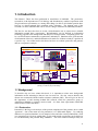
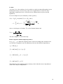
Genomics & Proteomics - tools to discover new target candidates
The principles
Genomics; to study effects at the mRNA level
Affymetrix chips
transcription
genes
(DNA)
translation
messenger
(mRNA)
modification
protein
control
• Sensitivity
(low mRNA concentration)
• High throughput
(40,000 mRNAs/analysis)
90
80
70
60
50
40
30
Experimental paradigm;
control vs. treated,
healthy vs. diseased
animals
Differences in
gene expression
(mRNA),
protein levels,
& protein
modifications
20
treated
10
0
A
B
C
D
y”
ntar
eme
mpl
o
c
“
Proteomics; to study effects at the protein level
Two -dimensional gel electrophoresis
Mass spectrometry
control
treated
• “Proteins do the job”
• Post-translational
modifications/regulations
• Body fluids
The workflow
Disease experts
Tech. experts
Genomics
Genomicsdata
data
Experimental
Experimentaldesign
design
obese
obesecontrol
control
Hypothesis
Hypothesis
obese
obesetreated
treated(PPAR)
(PPAR)
Proteomics
Proteomics data
data
Interpretation
Interpretation
(bioinformatics)
(bioinformatics)
↓↓
new
newknowledge
knowledge of
of
biological
biologicalpathways,
pathways,
mechanism
mechanismof
ofaction
action
of
ofdrugs
drugs
Targets!
Targets!
Figure 1.1 – The principles and workflow of a proteomic and genomic comparative study
(kindly provided by Björn Dahllöf)
1.1 Background
To describe why we have written this thesis, it is important to relate some background
information on the technologies that we base our work on. We also want to describe the
disease area connected with the insulin resistance syndrome (IRS). This will give an idea of
the importance of and meaning behind IRS research, which the proteomics group at
AstraZeneca Mölndal is primarily involved with. It is data from experiments within IRS
which we have used in our thesis.
1.1.1 Proteomics
Proteomics is the large-scale analysis of the protein complement of the genome, the so-called
“proteome”. One of the main uses for proteomics is in ‘differential display’. By studying
differences in protein abundance in cell samples before and after certain perturbations, (such
as a comparison of sick tissue with healthy, or sick with treated) conclusions can be drawn as
to cell functionality and potential drug candidates. The most common technique today for
4
this analysis is the use of 2D-PAGE (PolyAcrylamide Gel Electrophoresis) for separation
followed by Mass Spectrometry (MS) for identification. 1
In 2D-PAGE, proteins first migrate towards their iso-electric point along the pH scale (the
first dimension). In the second step the proteins are solubilized and evenly negatively
charged by the detergent SDS. When an electric field is applied, proteins will move through
the porous polyacrylamide gel with a speed inversely correla ted to their size, and the
separation will instead reflect their molecular weight (the second dimension).
After separation the gels are stained in order to visualize the protein spots, which are then
analysed using image analysis software tools. Usually the focus is on spots that differ
between different groups of samples, and their intensities can be compared and tested for
significance. The proteins in the interesting spots must be identified using MS before any
conclusions can be drawn.
There are commonly two MS identification methods in use today. The proteins are initially
digested in-gel. In Matrix Assisted Laser Desorption/Ionization – Time Of Flight (MALDITOF) the resulting peptides are then fired at by a laser and ionized so that they fly to a
detector, resulting in time of flight distributions according to their masses. These flight times
work as fingerprints which are searched against databases to finally determine the protein
identity. The second method uses two mass spectrometers in tandem (MS/MS) that ionize the
peptides by “electro spray” and break the peptides down into even shorter fragments that
allow for sequencing. This method is far more specific for identification than the MALDI
“fingerprint” method, but also more complex and time consuming. A recent development has
been a system that combines the two above mentioned techniques, thus benefiting from both
specificity and speed.
It should be mentioned that this relatively straightforward approach to protein expression
analysis can not identify and determine all proteins expressed in a cell at a given time point.
Only the most abundant spots (~20% of all proteins) are visible enough to be quantified, and
the interesting group of membrane proteins does not come out well at all on the gels. In
addition, proteins that have yet not been identified and annotated in databases can not be
determined using MALDI MS.
1.1.2 Microarrays
Microarray technology allows us to monitor the interactions among thousands of genes
simultaneously on a single chip. Hybridisation (i.e. base-pairing: A-T and G-C for DNA; AU and G-C for RNA) is the underlying principle of microarray technology. Arrays are
orderly arrangements of samples, and microarrays get their name from the very small sample
size, typically measured in 10s of microns. They provide a medium for matching known and
unknown DNA or RNA samples based on base-pairing rules. They require specialized
robotics and imaging equipment. The so-called “probe” is the tethered nucleic acid on the
microarray plate with known sequence, whereas the “target” is the free nucleic acid sample
whose identity/abundance is being detected (although this nomenclature is sometimes
reversed in literature). There are two major areas of application for the microarray
technology, identification of sequence (gene/gene mutation) and determination of expression
level (abundance) of genes.
The Affymetrix GeneChip is a microarray method invented by the company Affymetrix. The
GeneChip involves probes of oligonucleotides (25mer) synthesized in situ (on-chip).2 Instead
of using amplification techniques such as PCR, the oligonucleotides are synthetically
produced by the techniques of photolithography and solid-phase DNA synthesis directly on
the chip. This allows for the production of all possible combinations of sequences. The
chemical steps involved are:
5
1.
2.
3.
4.
Synthetic linkers with photochemically removable protecting groups are attached to a
glass substrate.
A filtering mask directs light to specific areas on the glass surface and thereby removes
the protecting groups.
Single deoxynucleosides with a protecting group, brought to the surface, bind to the
unprotected sites.
A new mask is applied and the procedure is repeated until a highly dense collection of
any desired oligonucleotides is obtained.
The array is then taken to a hybridisation chamber where fluorescent-labelled nucleotide
samples are injected and hybridised to the complementary oligonucleotides. Laser excitation
makes the samples fluorescent and a 2D fluorescence image of hybridisation intensity is
obtained by a scanner.
The short chains in the Affymetrix technique with only single points of constraint at either
end are highly accessible for hybridisation. This potentially allows for more accurate mRNA
quantification and the number of dynamic possibilities for detection increases. However,
disadvantages of the short-chain Affymetrix technique include the variations in melting
temperature due to AT-GC composition, and the reduction in specificity due to the small
number of nucleotides (~25).
The Affymetrix GeneChip is a very high-density microarray, where a single 1.28x1.28 cm
array today can contain probe sets for approximately 40,000 human genes and ESTs
(Expressed Sequence Tags). This compactness is advantageous because it allows more genes
to be analysed simultaneously. The use of perfect match probes as well as mismatch probes
(where a single nucleotide is substituted) greatly reduces the contribution of background noise
due to cross-hybridisation and increases the quantitative accuracy and reproducibility of the
measurements. These probe sets will be described in more detail in Section 2.3.2.
1.1.3 The Insulin Resistance Syndrome
One of the most rapidly increasing diseases among nations with a high standard of living is
Type II Diabetes Mellitus (T2DM). According to WHO (World Health Organisation), the
number of people affected will double up to 300 million within the next 25 years.3 Not only
today’s welfare states, but also developing countries with food and exercise habits resembling
the industrialized world’s, will see a dramatic increase of this disorder.
T2DM is preceded by insulin resistance, which means that the signalling properties of the
insulin molecules have less effect in the cell. Insulin is a peptide hormone whose main
function is to control
glucose levels in the blood,
and lack of these leads to
elevated glucose levels
with glucose intolerance
and diabetes as a result.
When the cells first
become less sensitive
towards insulin, pancreas
increases
its
insulin
production to overcome
the
“resistance”
and
thereby keeping blood
glucose on a normal level.
Eventually the insulin
producing ß-cells will
Figure 1.2 - The appropriate signalling through the insulin pathway is critical
for the regulation of glucose levels and the avoidance of diabetes4
6
become exhausted, the production will halt and diabetes evolves.
In addition to being a precursor to diabetes, the Insulin Resistance Syndrome (IRS) has other
serious implications, such as hypertension, atherosclerosis and dyslipidemia (high triglyceride
levels and low high-density lipoprotein levels) with probable cardiovascular disease as a
consequence.5 It is therefore obvious that a successful treatment of IRS would directly
improve the health of millions of people across the world and lower national medical costs.
Advances within this research have led to the discovery of a suitable target: The Peroxisome
Proliferator-Activated Receptors (PPARs). These are ligand-activated nuclear hormone
receptors that work as transcription factors bound to the DNA, ready to activate and regulate
genes responsible for glucose and lipid metabolism. There are three main types of PPARs:
PPARa, PPARd and PPAR? commonly present in different cell types.
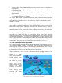
Peroxisome ProliferatorActivated Receptors (PPARs)
PPARs are nuclear receptors
(transcription factors) and “intracellular
sensors” of fatty acid levels
PPARα
liver
Fatty acids &
metabolites
PPARδ
ubiquitous
PPARγ
adipose tissue, liver
Regulation of genes in lipid and fatty acid metabolism
Synthetic activators of PPARs cause
normalization of dyslipidemia
PPARs exist as heterodimers together with
another nuclear receptor RXR and bind to
PPAR Response Elements (PPREs) in the
genes' promoter regions. When the genes
in question are inactivated a co-repressing
protein complex keeps the histones
deacetylated, thereby inhibiting transcription. If a ligand is added, a coactivating protein complex instead binds to
the PPAR-RXR heterodimer and the
histones are acetylated. This allows for
gene transcription.
Figure 1.3 – A picture diagram of PPARs
(kindly provided by Björn Dahllöf)
A certain group of small molecules have
proven to have activating ligand effects for
the PPARs, the so-called thiazolidinediones (TZDs). When insulin resistant obese and
diabetic animals are treated with these agents, insulin sensitivity and many of its other
associated pathological effects are normalized.
1.2 Purpose
The purpose of our thesis is to explore ways in which bioinformatics can be applied to
proteomics data and research to create additional value. The idea is that bioinformatics can
make current methods more effective and bring in new valuable information and
visualizations that can spark novel ideas for the researcher.
1.2.1 PPAR Response Elements
In a search for proteins that are up-regulated by PPARs, it is natural to ask the question:
“Which proteins have PPAR Response Elements (PPRE) in the promoter region of their
complementary genes?” PPREs are known to be a seat for the PPARs which induce
transcription. Response elements have a high degree of conservation and most of them have a
certain sequence motif. The PPRE is a so-called DR-1 motif, meaning a direct repeat of a
nucleotide sequence with one intervening nucleotide. The spacing nucleotide is usually an A
or T. The repeating sequence can also vary somewhat, although the consensus motif is
AGGTCA[AT]AGGTCA.6 Any promoter region with this DR-1 sequence has a high
likelihood of binding PPARs.
Localisations of PPREs in the promoter regions of a few known genes are described in the
literature. These are, however, not all the PPREs in the mouse genome and a method for
finding additional such response elements would be very desirable. If a method could be
developed into an automated application, it would be useful within biological research.
7
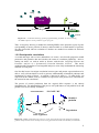
Drug
PPAR
gene
AGGTCA[AT]AGGTCA
PPRE
Promoter Region
mRNA
protein
Figure 1.4 – A schematic drawing of a drug ligand binding to PPAR, in turn activating
the PPRE sequence in the promoter region of a gene
Thus, we began by deriving a method for searching PPREs in the promoter region of genes
corresponding to mouse proteins of interest, and tested this on a small number of proteins.
We then proceeded with an evaluation of whether our method was suitable for full-scale
automation.
1.2.2 Gene/protein correlations
A second and larger task we have undertaken is to create a user friendly program to match
proteomics and genomics data and visualize the extent of correlation graphically. Prior to
starting our thesis, we read an article in Science with the title Integrated Genomic and
Proteomic Analyses of a Systematically Perturbed Metabolic Network.7 This article
emphasized the importance of an integrated analysis to more fully understand the interacting
networks in living cells.
Our idea has been to investigate correlation between gene and protein expression data to be
able to verify old conclusions as well as gain new understanding of metabolic pathways and
mechanisms of action of drugs. A question of interest for many is: “To what degree can
expression at the mRNA level be correlated to expression at the protein level, and what are
the reasons for non-correlation?”
The process of protein production from the original DNA sequence is not entirely
straightforward. An understanding of the process will yield hints as to why mRNA levels and
protein levels are not strictly correlated.
AFFYMETRIX
2D-PAGE / MS
Modified
protein
mRNA
?
protein
?
?
?
Degradation
DNA regulation
Figure 1.5 - Model of subsequent processes in a cell. Integrated expression analysis on both the
genomic and proteomic level can help in answering questions about the intermediary mechanisms.
8
The initial RNA molecule produced by transcription contains both intron and exon
sequences.8 Its two ends are modified, and the introns are removed by an enzymatically
catalysed RNA splicing reaction. The resulting mRNA is then transported from the nucleus
to the cytoplasm, where it is translated into protein. The final level of a protein depends on
the efficiency of each step and on the rates of degradation of the RNA and protein molecules.
Matchmaker
Comparing mRNA and protein data can give clues to answering the question marks in Figure
1.5 and ultimately lead to the localization of new and more effective drug targets. So what is
an effective way of producing and visualizing a comparison? Our answer to that question has
been to develop a program we have called Matchmaker.
Microarray analysis generates huge amounts of data. One chip detects the expression of
thousands of genes and ESTs. Proteomics does not operate on quite the same level, but there
are still potentially hundreds of protein spots. Matching these two manually is an extremely
time consuming process that would never be economically justifiable. Therefore, automation
in Matchmaker opens up the possibility of a comparison at minimal time-cost.
Creating an easy-to-use interface for the comparison has been a very important part of our
project. Without this, the program would not be used. We analysed what visualization
methods would be the most effective and what information these would entail. It was
important to receive feedback from the users. Through Matchmaker we have provided
researchers with a helpful tool in sparking new ideas and insight into the original data.
9
2. Analysis and Strategy
For a comparative analysis we needed an experiment conducted similarly on both the protein
and gene levels. There has been an interest for such a combination at AstraZeneca Mölndal,
but as of yet only a few of these studies exist. One such study, however, served as the testing
ground for our program, as well as the basis for the PPRE search. The chapter is divided into
a description of the study and an analysis of PPRE existence and gene/protein linkage
respectively.
2.1 The rosiglitazone study
The proteome study we have primarily looked at involves lean mice, obese control mice, and
obese mice treated with rosiglitazone (a TZD, see Section 1.1.3) for seven days.9 Tissue
samples from liver and white adipose tissue have been extracted. The treated group consisted
of four animals and the control group consisted of five animals. After image processing of
the fluorescently stained 2D gels, thousands of protein spots were readily quantified. From
these, hundreds of spots differed significantly from the control group spots according to a
Student’s t-test (P<0.05). 111 spots representing 58 unique proteins were identified by mass
spectrometry. Failures in spot identification were due either to very low chemical quantity of
the proteins, or to the lack of a hit in the databases queried. Although only proteins whose
expression showed significant changes were chosen, we were also able to include a number of
“unchanged” proteins in our analysis. The reason these had been identified was that they had
showed significant changes in the other comparison (lean vs. obese control).
The treatment effects of rosiglitazone were explored in a similar study at the mRNA level
with Affymetrix Mu6k chips (about 6000 genes/ESTs).10 Tissue samples were extracted from
liver, mesenterial fat, epididimys fat, brown fat and quadriceps. Groups of three mice were
treated one, three and seven days. The conditions were similar to the proteome study, except
for the fact that the mice were treated with ten times as high a dose.
We have used the obese treated vs. obese control comparison in liver tissue as our primary
means of testing our program.
2.2 PPRE
Before dwelling deeper into our methods, a few concepts used in bioinformatics need to be
explained:
•
EMBL (European Molecular Biology Laboratory) is a laboratory that maintains Europe’s
primary nucleotide sequence data resource. 11,12 The EMBL Nucleotide Sequence
Database is a comprehensive database of DNA and RNA sequences collected from the
scientific literature, patent applications and directly submitted from researchers and
sequencing groups. It collaborates with GenBank in the USA and the DNA Database of
Japan (DDBJ).
•
BLAST (Basic Local Alignment Search Tool) is a set of similarity search programs
designed to explore all of the available sequence databases regardless of whether the
query is protein or DNA.13 It uses a heuristic algorithm, which seeks local as opposed to
global alignments and is therefore able to detect relationships among sequences that
share only isolated regions of similarity.
10
•
ZSearch is a multiple sequence similarity search tool that performs similarity searches to
compare query sequences against a database of sequences. 14 It makes use of the BLAST
algorithm. Similarity searching is a key bioinformatics tool, enabling the identification
of regions of similarity between sequences that may indicate a shared structure or
function.
•
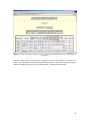
There are three types of quality classes assigned to sequenced genomic DNA.15 The first
two classes are found in the EMBL High Throughput Genome (HTG) division, while the
last class is moved to the Primary division (Figure 2.1). All first-time sequenced contigs
(pieces of cloned genomic DNA) greater than 2 kb get an accession number and are
deposited as Phase 1 sequence in HTG. This accession number never changes during the
following progress. The contigs are at that point unordered, unoriented and contain gaps.
As sequencing progresses the quality increases. Phase 2 contains ordered and oriented
sequences that may contain gaps. Finished sequences with no gaps belong to Phase 3
and are found in the Primary divisions (Rodent division in the mouse genome case).
Sequences in Phase 1 and 2 are also called “working draft sequences”.
Figure 2.1 – The orientation and relative size of contigs in the different
classes of the sequenced genome
In order to evaluate the possibility of an automated search for PPRE DR-1 sequences from an
initial list of interesting proteins, it was important to first derive a method for finding such
motifs. We used AstraZeneca’s Electronic Laboratory (E-Lab) 16 and the following work flow
to search for the DR-1 sequences:
1. The SWISS-PROT accession number is taken from an Excel sheet with a list of proteins
that are to be examined.
2. The SWISS-PROT entry is found using E-Lab. (In most cases, the protein was from
mouse, but could also be a rat or human homologue.)
3. On the entry’s DR-line (Database Reference) there are one or many links to the
corresponding genes’ EMBL entries. We always choose the first one.
4. This EMBL entry is BLAST searched via ZSearch, against the EMBL divisions Rodents
and High Throughput Genomes, to find genomic DNA that could contain a promoter
region for the gene in question.
5. A list of hits is produced and sorted according to Percent Identity (percentage of matching
nucleotides). Successful hits will be significantly longer than the query sequence since
genomic DNA that contains a promoter region as well as the coding region is needed.
The Query Percent (percentage of the total query sequence that was used in the match) is
another important value to look at. Since BLAST is a local similarity search tool, a hit
could match only one or a few of the exons within the gene, making the Query Percent
less than 100. Even if the hit only matches the first exon, we can still go further upstream
and look for the promoter region.
If the hit sequence is from Phase 1 or 2 in HTG it is very important to be aware of the size,
order and orientation of the contigs. Below is an example of an acceptable hit, although
the query sequence is quite short.
11
Score = 77.8 bits (39), Expect = 5e-14
Identities = 39/39 (100%)
Strand = Plus / Minus
Query: 1
gaaagatggcaccagttgctggcaagaaggccaagaagg 39
|| || | || || | || || | || || | || | || || | || || | || || | ||
Sbjct: 45710 gaaagatggcaccagttgctggcaagaaggccaagaagg 45672
Sbjct contig: 24863 - 66286: contig of 41424 bp in length
As can be seen in “Sbjct contig”, the contig has an uninterrupted section between the start
of the query gene and about 20 kb upstream. Thus, here is a proper location to search for
the DR-1. However, with the unfinished genome we can not be sure how large the
promoter region is, and where the previous gene ends. Therefore we scan 10 kb (10 000
nucleotides) ahead of the query match and assume that this covers most of the promoting
region. The problem is in some cases more complex than this; for example, certain parts
of a promoter region can exist hundreds of kb away from the gene. This is not something
we can take into account.
If a hit meets the criteria Percent Id > 95% (errors in sequencing taken into account),
Query Percent > 15%, and it contains genomic DNA about 10 kb (10.000 nucleotides)
upstream of the gene in a single contig (without gaps) it is fine to proceed. A contig must
thus contain both the beginning and the full promoter region of the gene to be valid for
further searching. It is not possible to jump to the next contig because there is a gap of
unknown size between the contigs.
6. When proper genomic DNA is found, ZSearch is used to search for the DR-1 motif. If a
hit coincides well with the consensus DR-1 it is likely to be a PPRE.
2.3 Matchmaker
To design a program that would automate the linkage between proteomic and genomic
expression, we needed to analyse the technologies behind the data to discover possibilities
and pitfalls.
2.3.1 2D-PAGE analysis
The Proteomics group uses a program called PDQuest to analyse spot intensities from 2Dgels. As an example, Figure 2.2 below shows 6 gels being matched in another study. The
left two gels are from obese mice, the middle two from lean mice, and the right two from
treated obese mice. After manual “landmarking” of a number of spots, the program attempts
to match the spots on the different gels automatically. However, there is a lot of manual
labour involved in checking that matches are correct and removing noise (spots that are
artefacts rather than proteins). The histogram in the figure represents one spot. Each bar
shows the intensity of that spot in one of the gels. In the example, the last six bars are the
treated obese gels and it can be seen that the protein is strongly up-regulated.
12
Obese
Lean
Treated Obese
Figure 2.2 – A PDQuest window where gels are being matched
(Kindly provided by Boel Lanne)
PDQuest has built-in statistical features, but the proteomics group instead uses an Excel
macro. The macro is based on the assumption that the logarithmic intensity values are
normally distributed, and can thus make use of Student’s t-tests to calculate a P-value (see
Section 2.3.4).
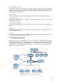
2.3.2 Affymetrix analysis
The Affymetrix system is built so that one DNA probe set is designed to detect one cRNA
transcript.17 A probe set usually consists of 16-20 probe pairs. A probe pair in turn consists of
two probe cells, a perfect match (PM) and a mismatch (MM). The PM probes are designed to
be complementary to a reference sequence. The MM probes are the same, except for a
homomeric base mismatch at the central position (e.g. 13th of 25 base length probe array).
These serve as a control for cross-hybridization.
Figure 2.3 – Affymetrix gene expression monitoring with oligonucleotide arrays. A single 1.28 x 1.28
cm array containing features smaller than 22 x 22 µm. Oligonucleotide probes are chosen based on
uniqueness criteria and composition design rules. For eukaryotic organisms, probes are chosen
typically from the 3´ end of the gene or transcript (nearer to the poly(A) tail) to reduce problems that
may arise from the use of partially degraded mRNA. The use of the PM minus MM differences
averaged across a set of probes greatly reduces the contribution of background and cross–
hybridisation and increases the quantitative accuracy and reproducibility of the measurements.2
13
Affymetrix uses a number of absolute analysis algorithms to compare the intensities of the
PM and MM probe cells to determine if a transcript is present (P), marginal (M), or absent (A;
undetected). This is called the Absolute Call. If, for example, the MM intensity is close to
the PM intensity, cross-hybridization is frequent, producing a lot of noise that makes the PM
intensity unreliable. When this is the case, the Affymetrix algorithms will tend to yield an A.
A metric that makes use of the probe cell intensities directly is the Average Difference. It is
an average of the differences between every PM probe cell and its control MM probe cell.
The Avg Diff is thus directly related to the level of expression of the transcript.
Affymetrix has designed a great number of additional metrics, but we have found Avg Diff
and Abs Call to be the most important for our purposes, and have chosen to rely on them for
further analysis. Together they allow for creation of an expression ratio, filtering of poor
data, and calculation of confidence intervals.
The probe sets on a GeneChip will naturally be of varying quality after an experiment has
been performed. Before matching the mRNA data with the protein data, it is preferable to
sort out the poor quality values from the mRNA data so that we get reasonably reliable plots.
We have done this by setting criteria on the Absolute Call: at least two thirds of the
experiments in one of the two cases compared (e.g. treated or untreated) must be P or M for
the probe set to be included. In other words, comparing treated and untreated with 3
experiments in each, we would accept values PPA/AAA and PPP/PPA, but reject PAA/PAA
and AAA/AAA. We have decided to keep cases such as PPP/AAA and vice versa even
though their Avg Diff ratios are unreliable, because they clearly imply an up- and downregulation respectively.
The Avg Diff values in Affymetrix experiments can sometimes be negative. This implies that
the average MM intensity is stronger than the average PM intensity for the probe set. An
explanation for this could be an extreme form of cross-hybridization where other transcripts
have lodged themselves on the MM probe. Another explanation could be that it is actually
the MM probe that is correct, and the PM instead acts as the mismatch. In either case, the
Avg Diff values can not be trusted. Essentially all negative values are labelled as A, so due to
our criteria we get rid of most of the negative values. The negative values left are included in
our calculations for statistical reasons. If they happen to make the entire average ratio
negative, the probe set will be excluded from the comparison.
Affymetrix has included a certain number of probe sets that do not follow their standard
selection rules. One example is an incomplete probe set, meaning that there are not as many
probe cells as usual. Another example is when a probe set is not specific enough to detect a
single gene, but rather a family of similar genes. We have decided to filter out these cases
from the comparison, since they would not give reliable values.
2.3.3 Matching genes and proteins
An Affymetrix probe set is designed to represent a gene or EST, and every gene codes for at
least one protein. Thus, we should in many cases be able to find a corresponding probe set on
an Affymetrix chip for every protein identified in a proteomics experiment. If the
experiments at the mRNA and protein levels respectively have been carried out identically or
at least in a similar fashion, it should be possible to directly compare the expression ratios for
the two levels. The advantage of using ratios in both cases is that it gives a relative measure
of the change in expression rather than an absolute measure, and thus is better suited for a
comparison.
Affymetrix supplies information on the reference gene/EST that each probe set represents.
The next step involves the decision on how to match the gene or EST with a corresponding
protein. The peptide masses from the mass spectrometry analysis are matched to a protein
14
database, and since this database primarily contains SWISS-PROT and TrEMBL entries, we
have decided to build our program to cope with these.
To check whether a gene matches a protein, a BLAST search must be done. After studying
the EMBL and SWISS-PROT/TrEMBL databases, we came across the fact that these
databases already are cross-referenced with each other. In the EMBL gene entry, the db_xref
row in an entry’s Feature Table section has a link to a SWISS-PROT /TrEMBL protein
accession number if the criteria are good enough. In the case of an EMBL EST entry, there
often exists a link in the Description (DE) row directly to protein, or to a gene which we can
further link to a protein. The above described method (without BLAST) is time saving and
easy to follow.
The use of the accession number in the linking is due to it being the “most unique” identifier.
Both the ID and AC rows are supposed to act as “unique” identifiers. However, the ID can
change due to its inherent construction. It is built up using an alphanumeric code (X_Y) that
is supposed to reflect the protein name and the species it comes from. “X” is a mnemonic
code of at most 4 alphanumeric characters representing the protein name (e.g. INS for
Insulin). “Y” is a mnemonic species identification code of at most 5 alphanumeric characters
representing the biological source of the protein. This code is generally made of the first
three letters of the genus and the first two letters of the species. If a protein is suddenly found
to belong to a different class or needs a new name, the ID can change.
“Accession numbers are the primary means of identifying sequences and provide a stable way
of identifying entries from release to release. For reasons of consistency it sometimes required
to change the entry name (ID) between releases (e.g. to ensure that related entries have similar
names). An accession number, however, always remains in the accession number list of the
latest version of the entry in which it first appeared. Accession numbers allow unambiguous
citation of database entries. Researchers who wish to cite entries in their publications should
always cite the first accession number in the list (the ‘primary’ accession number) to ensure
that readers can find the relevant data in a subsequent release. Readers wishing to find the
data thus cited must look at all the accession numbers in each entry's list. Secondary accession
numbers allow tracking of data when entries are merged or split. For example, when two
entries are merged into one, a new ‘primary’ accession number goes at the start of the list, and
those from the merged entries are added after this one as ‘secondary’ numbers.”18
With this in mind, linking genes and proteins by accession number is a safe method as long as
we make sure to check the entire row of accession numbers, not just the primary one. In
Appendix C, an example of an EMBL gene entry and its related SWISS-PROT protein entry
is shown.
2.3.4 Statistical considerations
To understand the underlying complications and limitations of the proteomics and genomics
technologies, some statistics is necessary. Of course to do a proper statistical comparative
study, experiments at both protein and mRNA level would have to be carried out in exactly
the same way. It would be ideal to use the same tissue, the same number of animals, the same
substance concentration, and so on. The primary studies we have to work with do not entirely
meet up to these criteria. However, our goal has been to get a statistical feel for the
technologies and also to come with suggestions on how to make future comparisons more
statistically significant.
The P-values used by Proteomics give a picture of whether a protein’s expression can be said
to be significantly changed. However, the P-value does not take into account the chance
occurrences of certain values that are likely to be present the more values we have. To then
get a proper idea of significance, an adjusted P-value should be used (see Appendix D).
15
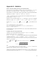
The confidence interval is a good measure to get an idea of the variance in a number of
samples. The 95% confidence interval, commonly used, gives us a region in which we could
find the point with 95% certainty given our experimental data. We have calculated
confidence intervals for both the proteomic and genomic variances and used somewhat
different formulas for the two levels (see Appendix D). Considering that the intensities are
skewed, we have assumed a log-normal distribution in the protein case. This method is not
possible for the Affymetrix intensity values (Avg Diff), because these can in certain cases be
negative. Instead we ha ve used an approximation called Fieller’s Theorem. 19
When the confidence intervals have been worked out, we have chosen to plot them along with
the average intensity values in log scale (those points with negative average genomic
intensities are filtered out prior to this). Log scale is more appropriate considering the span in
intensity values and also places points at the origin when expression is unchanged on both the
proteomic and genomic levels.
Affymetrix has, as described in a Section 2.3.2, several of their own statistical metrics for
their data. They do not, however, give a detailed explanation of the underlying statistics, and
can thus be hard to rely upon.
Worth mentioning is that we have not taken into account the inter-chip variation. This is the
variation within a single probe set, between the PM and MM values (see Section 2.3.2).
Knowledge of the intra-chip variation can affect the confidence interval in both directions, but
we did not consider it necessary to take into consideration for our purposes.
16
3. Program Design
This chapter discusses the design of our program Matchmaker. A section on usability is
followed by a description of the program’s functional and technical structure.
3.1 Usability
The usability aspect of our program was of primary importance. We felt the need to create a
clear, concise, attractive, and informative web interface to make the usage of the program
simple and pleasant.
3.1.1 User analysis
Matchmaker is intended for use primarily by the proteomics team (cell biologists). Molecular
biologists can also make use of the program. The users are not expected to have any
programming or UNIX experience, and thus a web interface is used and kept as simple and
clear as possible. The users have a good knowledge of the underlying biology and at least a
basic knowledge of both expression techniques, so these do not need to be explained in the
program.
3.1.2 System design
WEB INTERFACE
In the first stage of the program, the user must select the two studies to compare. The
genomics data is stored in databases. Thus, it was felt that building an invisible database
interface which would allow the user to select a study from the database list was the best
option.
Certain parts of a proteomics study are stored in a database, but the intensity values we
needed are not. Instead, this information is handled in Excel sheets. Since it was beyond the
scope of the project to expand the proteomics database to contain this data, we decided to
make use of a text area that the user can paste the data into. Copying from the Excel sheet to
the web page text area is easy and intuitive for the user. The user has to order the columns of
the sheet in a specific way so that the program understands the input. See Section 3.4 and
Appendix A for more detail.
VISUALIZATION
For the visualization, we wanted to be able to make 1D bar plots with error bars (the
confidence intervals) and 2D scatter plots with large flexibility in viewing the data. We found
Spotfire and Excel had these capabilities and were commonly used by our user group. We
decided to incorporate these two applications into the design of our program, with the benefits
of the power of the applications and their familiarity and accessibility within the user group.
Excel has good functionality with bar plots, allowing the user to easily create these plots with
the error bars using the values from the program results. Spotfire is a powerful visualization
tool. With the use of its Application Programming Interface (API), we were able to program
certain settings so that a scatter plot opens in the correct way with our result data at the click
of a button. All the result data is imported into Spotfire (not only the x- and y- values) so that
the user has the ability to view extensive information about points in the graph. The user also
has the ability to modify the plot in a number of ways throughout the analysis.
17
3.2 Functional structure
The following figure shows our design in functional terms.
Web Interface
Homepage (1)
Affymetrix
Selection
(3)
BDAT Database (6)
Protein
Pasting (4)
Central
Processing
(5)
EMBL Database (7)
Vis. Options
(11)
Spotfire
(12)
Help (2)
Visualization
of results (8)
Excel
(13)
Result
Guide (9)
Links to EMBL &
Swiss-Prot (10)
Figure 3.1 – Matchmaker’s functional structure from a user’s perspective
1. Homepage
The homepage is the user’s first view of the program Matchmaker. From here the user makes
his/her selections and can view the help section.
2. Help
This is a help section that describes what Matchmaker is capable of and a step-by-step guide
in using the program. The help section is embedded in the homepage, avoiding unnecessary
extra windows.
3. Affymetrix selection
The user must select which Affymetrix study to use in the comparison from the drop-down
menus.
4. Protein pasting
The user must also decide which protein study to use in the comparison. The data from this
study is pasted into a text area.
5. Central Processing
This is the core of the program where the proteomics and genomics studies are matched and
the results organized for subsequent presentation.
6. BDAT Database
BDAT stands for the Biological Data Analysis Team. After conducting an experiment, the
researchers working with genomics data extract the most useful information from the
Affymetrix databases and store it in the BDAT database.
7. EMBL Database
The protein-gene/EST links are found in EMBL entries.
18
8. Visualization of results
The results are shown in a table on the web page. There is a choice of further visualization
options in Spotfire and Excel. There are also hypertext links from each accession number to
AstraZeneca’s Electronic Laboratory (E-Lab), where AstraZeneca locally stores their version
of a number of public databases.
9. Result Guide
The result guide helps the user to understand the results and continue with further analysis.
10. Links to E-Lab
Each EMBL, SWISS-PROT or TrEMBL accession number has a hypertext link to the
database entry in E-lab.
11. Visualization Options
The visualization options in Excel or Spotfire are activated by pressing on the appropriate
button.
12. Spotfire
Spotfire.net Desktop 5.1 plots protein log-ratio against gene log-ratio. It is a powerful tool for
further graphical analysis.
13. Excel
Microsoft Excel 2000 is useful for viewing the data and adding/making adjustments. It is also
useful for creating bar graphs with error bars.
3.3 Technical structure
Matchmaker is built on a Perl platform. 20,21 The web interface is in HTML and CGI scripts
enable selection and forms.22,23 Perl DBI allows connection to an Oracle database and SQL
commands extract data from the Oracle database.24,25 SRS commands allow for connection to
the EMBL and SWISS-PROT/TrEMBL databases. The API scripts for accessing Spotfire
and Excel are written in VBScript.
MATCHMAKER.html
(1)
HTML
TITLE.html
(2)
HTML
MM_SELECT.pl
Perl DBI
(5)
FOOTER.html
(3)
HTML
HELP.html
(4)
HTML
Perl, CGI
BDAT (7)
(Oracle Database
with Affymetrix data)
Perl DBI
RESULT_GUIDE.html
(9)
HTML
MM_RESULTS.pl
(6)
Perl, CGI
SRS
VBScript
Hypertext Link
EMBL (8)
(Nucleotide Database)
EXCEL
(10)
SPOTFIRE
(11)
TEXT
FORMAT
(12)
E-LAB
(EMBL/SwissProt/
TrEMBL)
(13)
Figure 3.2 – Matchmaker’s technical structure
19
1. MM_FRAMES.html
An HTML file that defines the four frames of Matchmaker’s homepage.
2. TITLE.html
An HTML file that creates the title frame.
3. FOOTER.html
An HTML file that creates the footer frame.
4. HELP.html
An HTML file that creates the help frame.
5. MM_SELECT.pl
A Perl CGI and HTML file that controls the selection of genomics data. The connection with
the Oracle BDAT database is controlled us ing the Perl database interface (DBI). The choices
selected, as well as the protein data pasted into the text area, are saved as parameters that are
sent on to MM_RESULTS.pl.
6. MM_RESULTS.pl
A Perl and HTML file that matches the two data sets.
7. BDAT database
A denormalized Oracle database with Affymetrix data. The bioinformatics group has
extracted some of the more useful Affymetrix data into this database. BDAT table columns
include probe set name, time point, tissue, Avg Diff, Abs Call, and individual. The probe set
name has to be linked with another table that has the matching EMBL accession number for
each probe set.
8. EMBL database
Entries for all publicly known genes and ESTs are stored in this database.
9. RESULT_GUIDE.html
An HTML file that guides the user through the results with tips on how to analyse them.
10. E-Lab links
The accession numbers have hypertext links to E-lab, where the specific gene, EST or protein
entry can be studied in more detail.
11. Excel
The link to Excel is written in VBScript. It imports the data into an Excel sheet.
12. Spotfire
The link to Spotfire is also written in VBScript. It imports the data into a scatter plot.
Additional features using Spotfire’s API make sure that the axes are correct and that the
points are coloured by protein, and adjust the label density.
13. Text format
A link to the data in tabbed text format. This option is mainly available should the other
options fail.
20
3.4 User interface
The user’s first impression of the application is of great importance. Matchmaker’s
homepage is designed to be clear, simple, and informative (Figure 3.3). The initial web page
is built in four frames. The program logo is in the top frame, the program in the left frame,
and the help section in the right frame. At the bottom there is a frame with creator
information and links.
Figure 3.3 – Matchmaker’s selection page. Here the Affymetrix study has been chosen and the
proteomics data pasted in.
We have chosen to build the help section into the initial page for two main reasons: the
selection frame does not need the entire width of the page, and having the help section nearby
saves the user opening a new screen. The help section with a step-by-step guide through the
selection process can be found in Appendix A.
The results page (Figure 3.4) pops up when the user has submitted the selections and the
program has matched the genomic and proteomic data. On this page there is a link to a
Results Guide (see Appendix A). The guide explains the table columns as well as the
visualization possibilities. The guide would not fit on the same page as the results, because of
the size of the results table. We have chosen to make the Results Guide link open a new web
browser window so that the results page remains intact and can be viewed simultaneously.
21
Figure 3.4 – The results page shows the results in a table and contains the buttons for export to Excel
and Spotfire
From the results page, the data can be exported to Excel and/or Spotfire at the click of a
button. The large table contains all the protein spots that have been entered into the program
and the accompanying data, as well as genomic data if a match has been found.
22
4. Results
4.1 PPRE
We examined the same proteins that were identified in the study described in Section 2.1. In
most cases there were no acceptable hits against genomic sequences, since either the Percent
Id was too low or a long enough sequence of genomic DNA could not be found. When a hit
indeed was found it was usually a Phase 1 HTG sequence with too many gaps in the wrong
places, i.e. a continuous sequence long enough to hold a promoter region did not exist.
Consequently, no DR-1 motifs could be found in these proteins using the search method
mentioned above.
4.2 Matchmaker
After applying Matchmaker on the rosiglitazone study data sets, several proteins could be
linked to genes or ESTs. Of the 59 unique proteins from 86 different 2D gel spots, links to 30
genes and 2 ESTs were found. Thus, about half of the proteins could not be assigned to a
gene or an EST using Matchmaker’s algorithm. We have found three distinct reasons for this:
1.
A corresponding gene or EST was found on the GeneChip, but the criteria stated in
Section 2.3.2 had not been fulfilled since the proportion of Absent transcripts (A:s
rather than P:s) was unacceptable or the probe sets were not reliable in some other way
(7% of the non-linked proteins).
2.
The protein is a mouse protein, whose corresponding gene did not yet have a transcript
on this GeneChip Mu6k - versio n (55%). However, it is probable that these genes will
exist on later chip versions. For example, we found three of these transcripts in the
newer Mu11k (11 000 genes/ESTs) chip.
3.
The protein is not a mouse protein, but from another organism such as rat or human.
Mass spectrometry could not assign the protein to an entry in the mouse database and
therefore a homologue from a different organism with a good hit was chosen instead
(28% rats and 10% human).
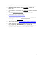
To visualize the gene/EST – protein links that were found, we used Matchmaker’s built-in
function buttons to transfer the result data to Spotfire and Microsoft Excel. Spotfire provides
various ways to plot the “Protein Log-Ratios” against the “Gene/EST Log-Ratios”, a couple
of which can be seen in Appendix B, Graphs 1-2 (B.1-B.2). However, visualizing the
confidence intervals was very complicated since an adequate tool does not yet exist in
Spotfire. It also proved to give messy and almost unreadable plots. Instead we plotted
confidence intervals in Excel, where they could easily be added using the error bar function in
a 1D bar diagram, with expression values from the proteins and their corresponding genes
plotted next to each other. Graph B.3 shows all genes and proteins, where spots from five
proteins have been merged.
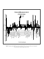
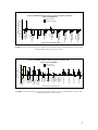
To reveal expression similarities in different groups of proteins/genes the diagrams were
divided according to protein classes. Graphs B.4-B.5 show similar behaviours in the groups
“Amino acid metabolism” and “Proven or presumed PPREs”.
Confidence intervals for eight genes were not calculated, since the statistical criteria in
Section 2.3.4 were not fulfilled. The only proteins without confidence intervals were the
merged protein spots, “merged” implying an average over all spots matched to the same
protein. Since there are dependencies between spots belonging to the same proteins, our
method for calculating confidence intervals is not adequate for the merged protein spots.
23
5. Discussion
5.1 PPRE
The main reason for not finding any DR-1 motifs was that the mouse genome is still incomplete.
When a genomic sequence region was found it was usually divided into unordered contigs,
which made the search for a promoter region impossible or at least very difficult. In order to
produce a fully automated DR-1 search tool, a search method had to be derived on the basis of a
test of a small number of proteins with known PPREs. Since the DR-1 motif was not found
even for these proteins, automation was not considered.
Currently the EMBL database contains very little genomic DNA. No valid hits were
generated starting from the proteins that were used in this study. To find any DR-1 regions in
the public genomic material that is present today, much handiwork as well as biological
knowledge and experience is needed.
A DR-1 search will most likely become easier in the future. The sequencing of the mouse
genome will proceed and the genome databases will be continuously updated. As of October
the 9th 2001, only 13.2% of the mouse genome exists as a working draft sequence and only
1.7% has been fully sequenced. 26 The working draft sequence of the mouse genome is
planned to be finished 2003, and the fully completed genome 2005. A complete and
annotated version of the mouse genome was recently made available from the genomic
company Celera. This sequence data is, however, only commercially available.
5.2 Matchmaker
CORRELATION
As can be seen in Graph B.1 expression levels for both protein and mRNA seem to be
moderately correlated, with R ˜ 0.5. This correlation coefficient suggests that mRNA and
protein levels are to some degree connected, but that they in certain cases are regulated by
more complicated mechanisms. A number of strongly up-regulated proteins with documented
PPRE regions in their complementary genes could not be matched in our program because
they were rat proteins. Had these been matched, they would most likely have increased the
correlation coefficient.
Nevertheless, a clear up- or down-regulation on both levels strengthens experimental results.
In addition, a direct correlation would theoretically suggest the possibility of using the gene
rather than the protein in pharmaceutical drug targeting. Knowledge of correlation can thus
be useful both in proteomics and genomics research.
REASONS FOR POOR CORRELATION
Even though it is natural to expect a correlation between mRNA and protein levels, there are
reasons why this is not always the case. There are known alterations that can occur in the
DNA>RNA>protein mechanism and that need to be considered. Post-transcriptional
changes refer to either degradation of mRNA or changes of the translational efficiency, i.e.
the efficiency by which mRNA is translated to proteins. Post-translational changes refer to
degradation or modifications of proteins.
Below are descriptions and possible explanations of drug effects and exceptions from the
“mRNA-yields-protein” relation:
24
1.
mRNA level unchanged, protein level up/down: The translational efficiency has
changed, which renders more or less protein from the same amount of mRNA (posttranscriptional). The protein is modified or degraded soon after translation (posttranslational).
2.
mRNA up/down, protein unchanged: Short lived mRNA does not have enough time to
produce sufficient amounts of detectable proteins (post-transcriptional). The protein is
produced, but is soon degraded or modified (post-translational).
3.
mRNA up, protein down or vice versa: More of mRNA is produced but the
translational efficiency is reduced even more or vice versa (post-transcriptional and
post-translational).
INDIRECT PPAR REGULATION
One explanation for up-regulation of genes, without PPREs in their promoter regions, is that
they can be indirectly influenced by “PPRE genes”. A drug ligand bound to PPAR, activating
a PPRE and inducing transcription could result in a gene product that is part of a different
gene regulating protein complex. The activation of a new promoter sequence, without PPRE,
would then lead to increased levels of other mRNA and ultimately to the production of other
proteins. Thus, there is a complicated network of “cause and effect”, which is far from
wholly understood.
FUNCTIONAL CATEGORIES
When studying expression levels of different functional categories, clear tendencies in
especially two categories are evident. Treating obese mice with rosiglitazone shows that
genes and proteins involved in amino acid metabolism are down-regulated on both levels
(Graph B.4). This effect has recently been shown and published. 27 The indication is that
PPARα is a key controller of intermediary metabolism during fasting. Graph B.5 indicates
that genes with proven or possible PPREs are up-regulated, although their corresponding
proteins are generally not as positively affected. Apparently there have been alterations in the
mRNA to protein chain.
Dividing and visualizing proteins according to functional categories can support thoughts
about which category non-classified proteins belong to. Points in a certain region of the plot
may have similar function. Thus, if a non-classified protein shows a similar expression
profile to a classified group of proteins, it may also belong to that group.
STATISTICAL COMMENTS
Regarding the statistical significance of the result data a few things need to be mentioned.
About 25% of the genes did not fulfil the statistical criteria for calculating reasonable
confidence intervals (see Appendix D). In addition, many of the calculated confidence
intervals were very large (see Graph B.3). These values reflect the limited reliability of the
Affymetrix microarray technique. In general, the confidence intervals for the protein
expression levels were not as wide as for the gene expression levels. The proteomics team
have done certain experiments to test the variance of the 2D-PAGE method. They have come
to the conclusion that the method’s coefficient of variance (CV, standard deviation/mean) is
around 20%. Similar experiments have been done with Affymetrix, but there the results
showed that the CV increased with decreasing intensity.28 For the majority of the intensity
values, CV was between 10% and 100%. The variance is clearly larger than in the
proteomics case.
In many cases with very wide or unreliable intervals there has been one specific mouse whose
mRNA expression value (Avg. Diff.) differs significantly from the others. Since there were
only three mice in each group, each individual has a large impact on the intervals. No matter
25
how accurate measurements will get, they will always reflect individual variance. Therefore,
it is important to conduct experiments with several individuals to acquire more statistically
significant results.
VISUALIZATION POSSIBILITIES
Through Matchmaker the user can export the result data to both Spotfire and Microsoft Excel,
which give excelle nt graphical representations when combined. By analysing the data from
the rosiglitazone study using Matchmaker we had the opportunity to explore suitable ways for
visualizing the results. An advantage with Spotfire is that every column in the original data
table can be used and displayed in the scatter plot itself, the “Query Devices” window and/or
the “Details-on-Demand” window. Size, shape and colour of the markers in the plot can all
represent different features (columns), simulating additional dimensions. New columns can
also be created by calculations or by binning (organizing data into “bins”) old columns.
These features allow the user to filter the data visually in ways that can highlight areas of
interest.
In Spotfire we coloured the markers according to protein accession numbers and used
different shapes for gene and EST transcripts. By binning the P-values in three groups
(<0.05;0.05-0.10;>0.10) and making check boxes of the groups it is easy to distinguish
proteins that are not changed significantly. The functional classes of the proteins were
denoted in “Comment1” and check boxes allowed for the choice of which protein classes to
be displayed. “Comment2” contained the reasons for why gene links to certain proteins were
not found, or whether a protein was merged or not. We have chosen to leave an unmerged
alternative, since there can be multiple reasons behind why the same protein has been
identified on many gel spots. Splitting could for example be due to natural degradation or
induced by the 2D-PAGE method.
As mentioned earlier, Spotfire is not yet suitable for visualizing confidence intervals,
especially when there are lot of markers. Excel, however, has a well developed functionality
for error bars, which can be used for confidence intervals in this case. Also here gene/protein
bars can be ordered into functional categories or any other suitable way.
A combination of scatter plots in Spotfire and bar diagrams in Excel creates a complete
method for visualizing the result data.
TECHNICAL LIMITATIONS
The Affymetrix technology will soon have the capability to fit essentially all of a mouse’s
genes on a GeneChip. The most recent chip fits 40,000 human genes, but has compromised
accuracy by reducing the number of probe cells for each probe set. The biggest problem in
the case of the mouse genome is that all genes have not yet been publicly sequenced.
The 2D-gel technique has limitations in the number of proteins that can be detected. A
dilemma exists between efficient protein quantification and detectability of proteins with a
very low concentration. Also, the proteome has not been fully established.
HOW PROTEOMICS CAN BENEFIT FROM M ATCHMAKER
Due to for example the statistical reasons mentioned above, the simultaneous expression
leve ls from proteomics and genomics experiments should not be blindly trusted. They may,
however, give useful indications, which can be more thoroughly investigated by examining
the raw data from the conducted experiments.
Global and integrated analyses are also important when investigating regulation and
interconnections within and between metabolic pathways in cells. In addition, Matchmaker
can be powerful when used as a verification of results in literature.
26
The comparative analysis has its greatest effect when using studies with the exact same setup. However, it can also be informative to compare two studies that are somewhat different,
but where the researcher for example knows that similar functions are affected in the body.
These could be used as more of a rough guide to check whether the genomic and proteomic
regulation are affected similarly.
5.3 Matchmaker in the future
In the rosiglitazone study neither the same tissue samples nor drug concentrations were used
in the two different experiments. It is naturally important for the biological relevance to have
the same conditions in both experiments in the future. Therefore, to be able to use
Matchmaker more precisely and with maximum benefit, coordinated studies must be strived
for.
If MS identif ication fails to identify a protein, a homologue from another organism is used if
the hit is good enough. However, Matchmaker can not match protein and genes from
different organisms. If a match still is desirable, the user has the choice of BLAST searching
for a hit with a worse score but from the correct organism. The new hit is probably not the
correct protein, but could be from the same family or at least have a similar function and
therefore be useful in further analysis.
Matchmaker will become even more useful in the future because:
1.
2.
3.
4.
More genomics and proteomics experiments will be coordinated.
The public gene and protein databases as well as the MS peptide database will grow.
The precision of the Affymetrix and 2D-PAGE/MS technologies is likely to improve.
More genes will fit on a chip, and ESTs will be replaced by genes.
We have thought of several developmental steps for Matchmaker that do not fit within the
scope of this thesis but that can be considered in the future.
•
•
•
Matchmaker can be more closely intertwined with the local information system
NEXIS (Next generation proteomics and EXpression Analysis Information System).
Links and cross-references to a variety of databases can be added, such as PDB
(Protein Data Bank) and Enzyme (Enzyme data bank).
If all proteomics data were inserted into AstraZeneca Mölndal’s Proteome Study
database (PS), Matchmaker could offer a selection system for this data in the same
way that it does for the genomics data. Pasting into the text area would then be
unnecessary.
27
5.4 Concluding remarks
•
Automating the process of finding PPRE motifs in the mouse genome proved not to
be feasible, primarily due to incompleteness of genomic mouse DNA.
•
Using Matchmaker on the comparison of obese mice with and without rosiglitazone
treatment showed that protein and gene expression levels were moderately correlated.
In certain cases this implies alterations in the “DNA to protein” process. In addition,
a number of expected trends were confirmed.
•
Matchmaker’s automated matching of gene and protein expression allows for quick
and easy comparative analyses of large data sets, making broader perspectives
possible. Analysis of the results will lead to new and useful hypotheses.
•
Integrated analysis of expression levels is important for the understanding of systems
biology, and will play an increasing role when more experiments become
coordinated, expression technologies are refined and sequence databases grow.
•
Matchmaker is a first step in making use of genomics and proteomics data
simultaneously. It has highlighted the potential benefits of such a comparison and
will lead the way for more such applications in the future.
28
Acknowledgements
We would like to give a special thanks to our supervisor Björn Dahllöf for his enthusiastic
support throughout the project.
We would also like to thank the following people for their help:
Anders Blomberg , our examiner.
Dept of Cell Biology&Biochemistry
Ulrika Edvardsson and Boel Lanne
Dept of Molecular Biology
Magnus Andersson, Anders Thelin, and Bengt Åsling
Dept of IS/IT (Disovery IS)
Frank Potthast, Petter Hallgren, Klaus -Hasso Schröter, and Hans Greberg
Dept of Biostatistics
Magnus Kjaer and Magnus Åstrand
29
References
1.
Wilkins, M. R. et. al. Proteome Research: New Frontiers in Functional Genomics.
Heidelberg: Springer-Verlag, 1997.
2.
Lipshutz, Robert J. et. al. ”High density synthetic oligonucleotide arrays”. Nature
Genetics 21, 1999. 20-24.
3.
Larsen, Henning. “Typ 2-diabetes: Livsstilssjukdom som ökar”.
NationalEncyklopedin Nytt. No. 3, 2001. 30-31.
4.
“BioCarta - Charting Pathways of Life”.
http://www.biocarta.com/pathfiles/insulinPathway.asp
5.
Olefsky, Jerrold M. et. al. “PPAR? and the Treatment of Insulin Resistance”. Trends
In Endocrinology and Metabolism. Vol. 11, No. 9, 2000.
6.
Schoonjans, Kristina et. al. ”Role of the peroxisome proliferator-activated receptor
(PPAR) in mediating the effects of fibrates and fatt acids on gene expression”. Journal
of Lipid Research. Vol. 37, 1996.
7.
Ideker, Tray et. al. “Integrated Genomic and Proteomic Analyses of a Systematically
Perturbed Metabolic Network”. Science. Vol. 292, 4 May 2001.
8.
Alberts, Bruce et. al. Essential Cell Biology. New York: Garland Publishing, 1998.
9.
Edvardsson, Ulrika. et. al. ”Rosiglitazone (BRL49653), a PPARy-selective agonist,
causes peroxisome proliferator-like liver effects in obese mice”. The Journal of Lipid
Research, Vol. 40, No. 7, July 1999.
10.
Thelin, Anders. “DNA array analysis of gene-expression changes in obese mice treated
with X103”. Molecular Biology, AstraZeneca R&D Mölndal, 1999.
11.
“EMBL - European Molecular Biology Laboratory”. www.embl.org
12.
Baxevanis, Andreas D. “The Molecular Biology Database Collection: an updated
compilation of biological database resources”. Nucleic Acids Research. Vol. 29, No.1,
2001. 1-10.
13.
“NCBI BLAST Home Page”. www.ncbi.nlm.nih.gov/BLAST
14.
“E-Help: ZSearch”. elab.rd.astrazeneca.net/cgibin/secure/incyte/srs5/help?context=ZSearch
15.
“High Throughput Genomic Sequences”. www.ncbi.nlm.nih.gov/HTGS
16.
“Bioinformatics HomePage”. elab.rd.astrazeneca.net
17.
Affymetrix. Microarray Suite User Guide. Version 4.0, 2000.
18.
“EMBL Nucleotide Sequence Database User Manual”.
www.ebi.ac.uk/embl/Documentation/User_manual/usrman.html
30
19.
Fieller, E.C. “The biological standardization of insulin”. Royal Statistical Society.
No. 7, 1940, Supplement. 1-64.
20.
Christiansen, Tom and Torkington, Nathan. Perl Cookbook. Sebastopol, CA:
O’Reilly, 1998.
21.
Schwartz, Ronald L. and Christiansen, Tom. Learning Perl. Sebastopol, CA: O’Reilly,
1997.
22.
Ronne, Erik. CGI Programmering med Perl. Stockholm: Docendo, 1998.
23.
“Sizzling HTML Jalfrezi - HTML by Example”.
freespace.virgin.net/sizzling.jalfrezi/iniframe.htm
24.
Descartes, Alligator and Bunce, Tim. Programming the Perl DBI. Sebastopol, CA:
O’Reilly, 2000.
25.
Connolly, Thomas et. al. Database Systems. Harlow, Essex: Addison-Wesley, 1996.
26.
“Mouse Genome Sequencing”. www.ncbi.nlm.nih.gov/genome/seq/MmHome.html
27.
Kersten, Sander et. al. ”The peroxisome proliferator-activated receptor α regulates
amino acid metabolism”. The FASEB Journal. Vol. 15, September 2001.
28.
Åstrand, Magnus. “Analysis of sources of variation in connection to chip array gene
expression experiments”. Biostatistics, AstraZeneca R&D Mölndal, 2000.
31
Appendix A - User Documentation
A.1 Introduction
WHAT DOES M ATCHMAKER DO?
Matchmaker starts out by asking for an Affymetrix and a proteomics data set to compare. The
Affymetrix data set is chosen as a specific table in the BDAT Oracle database, while the
Proteomics data set is pasted into a text area in a specified format. In the bulk of the program
proteins are matched with their respective genes or ESTs and the result is displayed onscreen. There is a link to the data where it is temporarily stored as a text file, and button
options that export the data to Excel and Spotfire. Excel is primarily used to add comments
and be able to save the results, as well as to create bar plots with errors bars. Spotfire is used
for plotting the data 2-dimensionally and analyzing further.
TECHNICAL D ESCRIPTION
Matchmaker consists of a web page (HTML) where selections of genomics and proteomics
data are made, and a web page with results and visualization options. Perl CGI scripts run in
the background to insure interactivity, and also to match the data sets. The connections to the
Oracle databases are handled using SQL commands with the Perl Database Interface (DBI),
and SRS commands allow for connection to the EMBL and SWISS-PROT/TrEMBL
databases. The Excel and Spotfire visualization buttons are programmed with VBScript.
LOCATION
Matchmaker is available on AstraZeneca Mölndal’s intranet at the address (URL):
http://bioinfo.seml.astrazeneca.net/farmmc/matchmaker.html
A.2 System requirements
The program is designed to run faultlessly in the Topaz environment, AstraZeneca’s global
Windows 2000 pla tform. Topaz has Internet Explorer 5.0.
The program relies on the bioinformatics group’s BDAT server to be available and kept
standardised. The program also relies on the availability of the local SRS system for
accessing EMBL, SWISS-PROT, and TrEMBL entries.
For the visualization options in Excel and Spotfire respectively, these applications must be
installed on the computer.
A.3 Step-by-step guide
This is a step-by-step guide to the selection process.
Step1: Affymetrix - Choice of disease area
The first thing to do is to choose the Affymetrix disease area to compare with. Simply select
one from the pull-down menu.
Press “Next”
Step2: Affymetrix - Choice of particular study/tissue
32
Choose the Affymetrix study to compare with. Simply select one from the pull-down menu.
Press “Next”
Step3: Affymetrix - Choice of the time point ratio
Choose two treatment days to produce a ratio. For example, "treated day 7 vs. untreated"
would mean choosing 7 for time point 1 and 0 for time point 2.
Usually you will be wanting to compare studies of exactly the same type in Affymetrix and
proteomics. Thus, make sure that also the ratios are inserted into the program in the same
way (e.g. treated vs. untreated).
Press “Next”
Step4: Name of output file
Write in a name for your result file. The results will be temporarily stored in this name on a
UNIX disk. To safely keep the results for future use, please save them on your own disk
afterwards.
Press “Next”
Step5: Proteomics - Insertion of data
Now it's time to insert the proteomics data. The data has to be in a specified format to be
properly understood by the program.
The file can be created in Excel (or saved as a text file) and then copied and pasted into the
text area on the web page.
Important:
•
•
•
Make sure that all 10 column headings are entered even if they don’t contain any
data. Also, make sure that the columns are in the correct order and that the heading
of the first column is "SSP".
Make sure there are no line feeds anywhere within a column (do not press enter or tab
when typing in a cell).
The program requires the logged average intensities.
Finally, press “Submit”. The program will now start processing the input. It could take
several minutes for the results to appear.
A.4 Result guide
This guide describes the results and the options for visualization of the results.
The results are shown in a large table (see Column Description below). There is also a small
table with the following information:
•
•
•
•
# of protein spots: Tells us how many different protein spots were pasted into the text
area.
# of unique proteins: Several spots can be the same protein, so the number of unique
proteins is less than the number of spots.
# of gene-protein links: The number of unique gene-protein links. The number in
parentheses refers to the spots for each protein being separately counted.
# of EST-protein links: The number of unique EST-protein links. The number in
parentheses refers to the spots for each protein being separately counted.
Besides the two tables in the browser, you have three more alternatives for viewing the results
(all at the top of the page):
33
•
•
The first button opens an Excel sheet with the data. Excel is primarily used to add
comments and be able to save the results, as well as to create bar plots with errors
bars. Please save your data in Excel onto your own M-drive!
The second button opens Spotfire and plots the data immediately (Protein log-ratio
vs. Gene/EST log-ratio). This 2-dimensional plot can then be manipulated in many
ways for further analysis.
You can save your Spotfire plot in two ways:
•
•
Saving as a Spotfire Analysis File (*.sfs) will save the plot and the data.
Saving as a Spotfire Template File (*.sft) will only save the adjustments you have
made to the plot. This is a good alternative if, after making adjustments, you would
like to add some more information to the data (e.g. in Excel) and then reinsert the
data into Spotfire.
The third alternative is primarily for use if the first option for some reason doesn't work. You
can click on the link with the name of your output file, and it is then shown as a tabbed text
file in the web browser. From here you can save the file by choosing "File/Save As" in the
web browser.
Column description
The large result table has several columns:
•
•
•
•
•
•
The Proteomics columns initially pasted into the text area carry through and appear in
the table. Each protein accession number is a hypertext link to the SWISSPROT/TrEMBL entry in E-Lab.
The "EMBL accession number" is the gene or EST link to the protein. If no link was
found, this will be stated. Each EMBL accession number is a hypertext link to the
EMBL entry in E-Lab.
A "Type" column has been added to show whether the link is with a gene or an EST.
There are three columns for the gene/EST log-ratio and its lower and upper bound
according to a 95% confidence interval. In some cases the interval does not satisfy the
criteria of the statistical method, and in these cases no interval will be shown
(interpret as interval being too big). The interval is based on the inter-chip spread
(essentially the variation in individuals) and does not take into account the intra-chip
spread (within the probe sets).
The "Absolute Call" column refers to an Affymetrix statistically based call, that
decides on whether it thinks the correct mRNA has indeed attached to the probe set.
"A" means absent, "M" means marginal, and "P" means present. The ratio you see
shows each mouse (chip) in the two time points respectively. Our criteria for this is
that at least 2/3 of the chips in either the first or the second time point are "P" or "M".
Otherwise the gene/EST will not be shown, even if it could be linked to a protein.
Don't forget that you can add useful comments into the "Comment1" and
"Comment2" columns before or after running the program!
34
Appendix B – Result diagrams
Graph 1 – Scatter plot where the colours represent protein
names and the shapes whether the mRNA molecules are
genes or ESTs. Ratios refer to treated/untreated. The
straight line is a least squares fit. Five proteins have more
than one spot, and these spots have been merged.
Graph 2 – Same as in Figure 1 except that no protein spots
have been merged.
35
Expression Ratio
-0.3
-0.8
-1.3
Proteins with corresponding genes
Graph 3 – Bar diagram of protein and mRNA expression ratios (treated/untreated). The error bars represent confidence intervals when applicable
Only expression ratios for unique and merged protein spots are shown.
regucalcin
2-oxoisovalerate
dehydrogenase E1-aATP synthase alpha
chain
ATP synthase alpha
chain
adipophilin
peroxiredoxin 1***
14-3-3 protein
zeta/delta
carbonic anhydrase III
actin, gamma1
MERGED epoxide
hydrolase
MERGED catalase
glutathione stransferase 5
60 kDa heat shock
protein, mitoch. prec.
78kda glucose
regulated protein prec.
prohibitin (b-cell
receptor associated
Apolipoprotein E
Apolipoprotein E
Apolipoprotein E
Apolipoprotein E
glyceraldehyde 3phosphate
MERGED
hydroxymetylglutarylnadp-dependent malic
enzyme***
MERGED fatty acid
synthase
pyruvat carboxylase
aspartate
aminotransferase,
ornithine
carbamoyltransferase
phenylalanine-4hydroxylase
argininosuccinate
synthase
ornithine
aminotransferase
MERGED 4hydroxyphenylpyruvate
acyl-coa
dehydrogenase, veryacyl-coa
dehydrogenase, longlong-chain-fatty-acid-coa ligase 2
fatty acid binding
protein, intestinal(I-
1.2
Protein and mRNA expression ratios for
all functional classes
Protein-LogRatio
Gene-LogRatio
0.7
0.2
Expression LogRatio
-0.1
-0.2
-0.3
-0.4
Apolipoprotein E
Apolipoprotein E
Gene/ EST Log-Ratio
Apolipoprotein E
Protein Log-Ratio
0.4
Apolipoprotein E
0.5
MERGED
hydroxymet
ylglutaryl-CoA
synthase
hydroxymet
ylglutaryl-CoA
synthase
MERGED 4hydroxyphenylpyruvate
dioxygenase
4hydroxyphenylpyruvate
dioxygenase
4hydroxyphenylpyruvate
dioxygenase
4hydroxyphenylpyruvate
dioxygenase
ornithine
aminotransferase
precursor
argininosuccinate
synthase
phenylalanine-4hydroxylase
1
hydroxymet
ylglutaryl-CoA
synthase
-1
ornithine
carbamoyltransferase
precursor
0.8
hydroxymet
ylglutaryl-CoA
synthase
-0.8
fatty acid binding
protein, intestinal(IFABP)
-0.6
acyl-coa
dehydrogenase,
very-long-chain
specific, mito.
acyl-coa
dehydrogenase,
long-chain specific,
mito.
-0.4
aspartate
aminotransferase,
cytoplasmic
-0.2
long-chain-fatty-acid-coa ligase 2
Expression LogRatio
Protein and mRNA expression ratios for genes and proteins involved in
Amino acid metabolism
Protein Log-Ratio
0.6
Gene/ EST Log-Ratio
0.4
0.2
0
Proteins with corresponding genes
Graph 4 – Expression ratios for genes and proteins involved in amino acid metabolism. Proteins with
with and without merged spots are shown.
Protein and mRNA expression ratios for genes and proteins with
proven or presumed PPRE
0.3
0.2
0.1
0
Proteins with corresponding genes
Graph 5 – Expression ratios for genes and proteins with proven or presumed PPRE. Proteins with
and without merged spots are shown.
37
Appendix C – EMBL and SWISS-PROT Entries
EMBL gene entry
In one of the feature table (FT) rows there is a cross-reference (db_xref) to a SWISS-PROT
entry with the corresponding protein.
-----------------------------
ID MMADFP standard; RNA; ROD; 1680 BP.
XX
AC M93275;
XX
SV M93275.1
XX
DT 15-MAY-1992 (Rel. 31, Created)
DT 04-MAR-2000 (Rel. 63, Last updated, Version 3)
XX
DE Mouse adipose differentiation related protein (ADFP) mRNA, complete cds.
XX
KW adipose differentiation-related protein.
XX
OS Mus musculus (house mouse)
OC Eukaryota; Metazoa; Chordata; Craniata; Vertebrata; Euteleostomi; Mammalia;
OC Eutheria; Rodentia; Sciurognathi; Muridae; Murinae; Mus.
XX
…
DR
DR
XX
FH
FH
FT
FT
FT
FT
FT
FT
FT
FT
FT
FT
FT
FT
FT
FT
FT
FT
FT
FT
FT
FT
FT
FT
FT
FT
FT
FT
FT
XX
SQ
MGD; MGI:87920; Adfp.
SWISS-PROT; P43883; ADFP_MOUSE.
Key
Location/Qualifiers
source
1..1680
/db_xref="taxon:10090"
/organism="Mus musculus"
/strain="C3H"
/cell_line="1246"
/tissue_type="adipose"
5'UTR
1..78
/note="putative"
mRNA
1..1680
/evidence=EXPERIMENTAL
CDS PEPT
79..1356
/codon_start=1
/db_xref="SWISS-PROT:P43883"
/evidence=EXPERIMENTAL
/standard_name="ADRP"
/gene="ADFP"
/product="adipose differentiation related protein"
/protein_id="AAA37176.1"
translation="MAAAVVDPQQSVVMRVANLPLVSSTYDLVSSAYVSTKDQYPYLRS
AEKGVKTVTSAAMTSALPIIQKLEPQIAVANTYACKGLDRMEERLPILNQPTSEI
VTGAKDVVTTTMAGAKDSVASTVSGVVDKTKGAVTGSVERTKSVVNGSINTV
VGPFYPQSTEVNKASLKVQQSEVKAQ"
3'UTR
1357..1680
/note="putative"
polyA_signal 1664..1669
/note="putative"
polyA_site 1680
Sequence 1680 BP; 422 A; 413 C; 460 G; 385 T; 0 other;
agtggtgatctggaccgtgcggacttgctcgtccc……………………..
38
SWISS-PROT e ntry
The following SWISS-PROT protein entry corresponds to the EMBL gene entry above.
-----------------------------
ID
AC
DT
DT
DT
DE
GN
OS
OC
OC
OX
RN
RP
RC
RX
RA
RT
RT
RL
RN
RP
RC
ADFP_MOUSE STANDARD;
PRT; 425 AA.
P43883;
01-NOV-1995 (Rel. 32, Created)
01-NOV-1995 (Rel. 32, Last sequence update)
30-MAY-2000 (Rel. 39, Last annotation update)
Adipophilin (Adipose differentiation-related protein) (ADRP).
ADFP OR ADRP.
Mus musculus (Mouse).
Eukaryota; Metazoa; Chordata; Craniata; Vertebrata; Euteleostomi;
Mammalia; Eutheria; Rodentia; Sciurognathi; Muridae; Murinae; Mus.
NCBI_TaxID=10090;
[1]
SEQUENCE FROM N.A.
TISSUE=Adipocyte;
MEDLINE=92390349; PubMed=1518805;
Jiang H.P., Serrero G.;
"Isolation and characterization of a full-length cDNA coding for an
adipose differentiation-related protein.";
Proc. Natl. Acad. Sci. U.S.A. 89:7856-7860(1992).
[2]
SEQUENCE FROM N.A.
STRAIN=C3H; TISSUE=Adipose tissue;
…
CC -!- FUNCTION: MAY BE INVOLVED IN DEVELOPMENT AND MAINTENANCE OF
CC
ADIPOSE TISSUE.
CC -!- SUBCELLULAR LOCATION: MEMBRANE-ASSOCIATED.
CC -!- TISSUE SPECIFICITY: ADIPOSE TISSUE SPECIFIC. EXPRESSED ABUNDANTLY
CC
AND PREFERENTIALLY IN FAT PADS.
CC -!- INDUCTION: BY DEXAMETHASONE.
CC -!- SIMILARITY: BELONGS TO THE PERIPILIN FAMILY.
DR EMBL; M93275; AAA37176.1; -.
DR EMBL; L09734; -; NOT_ANNOTATED_CDS.
DR MGD; MGI:87920; Adfp.
DR InterPro; IPR004279; perilipin.
DR Pfam; PF03036; perilipin; 1.
KW Membrane.
SQ SEQUENCE 425 AA; 46664 MW; 82624E6CE3429C22 CRC64;
MAAAVVDPQQSVVMRVANLPLVSSTYDLVSSAYVSTKDQYPYLRSVCEMAEKGVKTVTSA
AMTSALPIIQKLEPQIAVANTYACKGLDRMEERLPILNQPTSEIVASARGAVTGAKDVVT
TTMAGAKDSVASTVSGVVDKTKGAVTGSVERTKSVVNGSINTVLGMVQFMNSGVDNAITK
SEMLVDQYFPLTQEELEMEAKKVEGFDMVQKPSNYERLESLSTKLCSRAYHQALSRVKEA
KQKSQETISQLHSTVHLIEFARKNMHSANQKIQGAQDKLYVSWVEWKRSIGYDDTDESHC
VEHIESRTLAIARNLTQQLQTTCQTVLVNAQGLPQNIQDQAKHLGVMAGDIYSVFRNAAS
FKEVSDGVLTSSKGQLQKMKESLDEVMDYFVNNTPLNWLVGPFYPQSTEVNKASLKVQQS
EVKAQ
39
Appendix D - Statistics
Fieller’s Theorem (confidence intervals for the Affymetrix data)
Fieller’s theorem is used in finding a confidence set for a ratio of paramaters, ρ = θ1 / θ2 . In
general there are two statistics, θˆ1 and θˆ2 , which estimate θ1 and θ2 , respectively. It is
assumed that (θˆ1 , θˆ2 ) follows either exactly or approximately a bivariate normal distribution
with mean (θ1 , θ2 ) with σ11 = var(θˆ1 ), σ22 = var( θˆ2 ), σ12 = cov( θˆ1 ,θˆ2 ).
…With t1-α/2 (d) denotin g the 100(1-α/2)th percentile of the t distribution with d degrees of
freedom, P[H(ρ)2 ≤ t1-α/2 (d) 2] = 1 - α. (1)
Equation (1) can be rewritten as P(Q(ρ) ≤ 0) = 1 - α, where Q(ρ) = f0 -2f1ρ+f2ρ 2 is a quadratic
function of ρ, with f0 = θˆ12 - t1-α/2 (d) 2 σ̂ 11 , f1 = θˆ1 θˆ2 - t1-α/2 (d) 2 σ̂ 12 , and f2 = θˆ22 - t1-α/2 (d) 2 σ̂ 22 .
Defining D = f 12 − f 0 f 2 , r1 = ( f1 − D ) / f 2 , r2 = ( f 1 + D ) / f 2 , the confidence set for
ρ is:
Case 1: A finite interval [r1 ,r2 ], if D ≥ 0 and f2 ≥ 0.
Case 2: The complement of a finite interval, (-∞, r2 ] ∪ [r1 , ∞), if D ≥ 0 and f2 < 0.
Case 3: (-∞, ∞) if D < 0 and f2 < 0.
So for our purposes, the equation must fulfil the Case 1 criteria for the confidence interval to
be used in the plots.
Confidence intervals for the proteomics data
Assuming X has a log-normal distribution, then ln( X ) ~ N ( µ , σ 2 ) , i.e. normally
distributed with expected value µ and variance σ 2 .
Let X 1 ,K , X n och Y1 , K, Ym represent random samples from two log-normal distributions.
Assuming also that ln( X i ) ~ N ( µ X ,σ 2 ) and ln( Yi ) ~ N ( µ Y ,σ 2 ) , we have a 95%
confidence interval for the estimate of the difference (on the log scale) between the expected
values µˆ X − µˆ Y given by
1 n
1 m
ln( X i ) − ∑ j=1 ln( Y j ) ± t1−0.05 / 2 ( n + m − 2) ⋅ s pooled ⋅ 1 / n + 1 / m
∑
i =1
n
m
where
s pooled =
( n − 1) ⋅ s X + ( m − 1) ⋅ sY
n+ m− 2
and
s X , sY are the standard deviations for the random samples, t1−0.05 / 2 ( n + m − 2) is the 97.5%
quantile from the t-distribution with m+n-2 degrees of freedom.
Taking the anti-logarithm of the end points in the interval above we get a confidence interval
~ ~
for the quotient between the medians X / Y = e µ X / e µY to our two log-normal distributions.
40
P-values
A p-value αˆ ( x) is the smallest α level on which we could reject the null hypothesis, given
the data that we have received. The p-value is not a significance level since it is datadependent (a significance level α is the risk we are willing to take to reject a true null
hypothesis).
For a two sample t-test (two-sided) the p-value is given by
αˆ ( x ) = Pθ ( H 0 is rejected | T ( x) = t , H 0 is true )
T (x)
= 1−
∫
T (x)
dF ( y ) = 1 −
−T ( x )
∫
−T ( x )
ν + 1
 ν +1 
Γ

2 − 2 




2
1
+
y



dy

ν  ν 
νπ Γ 
2
where ν is the degrees of freedom, Γ( z ) is the Gamma function and
T ( x) =
x1 − x 2
s pooled
1 1
+
n1 n2
.
The above integral is solved numerically.
Holm’s step-down method (adjusted p-values)
Let p1 , p 2 ,K , p k denote the original p-values, sorted in ascending order, that have been
received from k hypothesis tests, the adjusted p-values are then defined sequentially by
~
p1 = min {kp1 ,1}
~p = min {max {~
p1 , ( k − 1) p 2 },1}
2
M
~p = min {max {~p , ( k − j + 1) p },1}
j
j −1
j
M
~
p k = min {max {~
p k −1 , pk },1}
This method is used in multiple testing to adjust p-values when the tests are dependent (it
works even if they are independent).
41