Download User manual v1.0

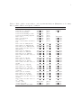
1
User Manual for the Spiking Neuron Basal Ganglia Model
Version: 1.0 14/12/2006
Mark D. Humphries
[email protected]
Abstract
The spiking neuron model of the basal ganglia was developed over a period of 6 years,
and the resulting code-base reflects the complexity of this process. These notes are intended
to guide the end-user through the basic structure and use of the code. Please e-mail any
suggestions, requests, or queries for incorporation into future revisions.
1
Introduction
The following is a short user manual for the spiking neuron basal ganglia (BG) model, guiding
the user through the basic steps of calling the correct functions, and how the results presented in
the Journal of Neuroscience paper (Humphries et al., 2006) were analysed. It is anticipated that
the copious Help sections and comments throughout the code will be sufficient to understand
the detail.
All names in bold are MATLAB functions or scripts. All custom MATLAB functions have
full Help comments describing their function calls. The code is provided in exactly the form in
which we used it, and so there are some inevitable historical oddities (comments not matching
text, redundant parameters etc). Nevertheless, by doing this we can ensure that our results are
replicable!
Unpack both ZIP files to a single directory, then add that directory and all its sub-directories
to your MATLAB path.
2
Basic code
The central function is BATCH BG heterogenous AMPA NMDA, which accepts five arguments including a string containing the filename of the parameters file. Every user-definable
parameter is contained in this file, so that BATCH BG heterogenous AMPA NMDA
only requires editing if new structures (e.g. thalamus, cortex) are added to the model. A second version BATCH BG heterogenous AMPA NMDA2 has the additional flexibility of
assigning separate weights to the AMPA and NMDA receptors, though this was only used in
(Humphries et al., 2006) to study the effects of NMDA receptor blockade on the γ-band activity.
These functions call in turn:
1. BG GHS input, which generates the cortical input streams according to the values set
in the parameters file.
2. BG net shunt AMPA NMDA, which creates the network specified in the parameters
file. The random number generator is reset before this function is called to ensure that
the same network is specified each time for a given parameter set. In turn, this function
calls
• PSPtoPSC, which converts the post-synaptic potential size, give in volts within
the parameters file, into the appropriate current step that should be elicited by the
arrival of a spike at the pre-synaptic membrane (given the post-synaptic neuron’s
average membrane properties).
2
3. GHS LIF solver shunt AMPA NMDA, which simulates the specified network for
the specified time period, given the specified inputs. This is a MEX-file, compiled from
the original C. Compiled versions exist for Windows XP, Linux, and 64-bit Linux, but
compiling a MEX file for any system is straight-forward.
2.1
The parameters file
A full parameters file is typified by the pars script. The most altered parameters appear at
the top of the file, including global dopamine level, simulation time, and input type and rates.
After this is a section which specifies the global network parameters (number of neurons per
channel, and so on), followed by parameters for each class of neuron. These are followed by
weights and transmission delays, coefficients for the STN and GP dopamine models, shunting
inhibition parameters, intrinsic currents (driving spontaneous and burst firing), and the option
of including injection currents.
All parameter values are given in SI units (seconds, amps, volts etc) where required. This
avoids the inevitable errors that occur in the worryingly common practice of working in “physiological” units (ms, pA, mV etc).
2.2
Undocumented parameters
There are some parameters in the code that are not mentioned in (Humphries et al., 2006)
because they were not used. However, they may be useful in future experiments, and so we
briefly describe them here.
1. trace n the neuron given here (e.g. GPe(75) is the 75th GPe neuron) has complete traces of
some of its variables saved in the results file from BATCH BG heterogenous AMPA NMDA.
gabaa
The current list is: distal inhibitory synaptic input Ij∈∆
, membrane potential V m , and
i
total gating variable Qh . The variables that are saved can be edited in
GHS LIF solver shunt AMPA NMDA, and a commented-out list of suggestions is
included in that code (don’t forget to re-compile after editing).
2. ref resets the membrane potential to this value after a spike is fired. This allows for explicit
after-hyperpolarisation to be modeled if required, though does introduce small numerical
errors as the analytic solution to V m does not account for this.
3. STN ext ratio will scale the cortical-subthalamic weight to be this fraction of the corticalstriatal weight.
4. PSP sigma standard deviation of (normally-distributed) noise for post-synaptic potential
size. Allows for separate parameterisation of synaptic noise (due to e.g. spike failure or
graded vesicle release) from membrane noise.
5. Injection current (end of script): the simulation code contains the ability to inject a
current pulse train of specified width and frequency into user-selected cells. This allows
for simple replications of current injection studies in intact BG.
2.3
The simulation engine
Our central simulation engine GHS LIF solver shunt AMPA NMDA was written in C to
gain a vast performance increase over native MATLAB code. It uses a mixed time-driven/eventdriven system, where each neuron’s membrane potential is updated every time-step, but its
synaptic input is only processed when an pre-synaptic event occurs (and accounting for the
transmission delay). We feel this achieves a good trade-off for analytically solvable model
3
neurons between the flexibility of a time-driven system and the efficiency of an event-driven
system.
The C code was written for optimal performance, and as such is not particularly humanreadable. We made full use of the analytically solvable neuron model by moving all constants
outside of the neuron update loop (they are computed in BATCH BG heterogenous AMPA NMDA
before the simulation engine is called). This enabled us to achieve faster than real-time performance (i.e 5 seconds of simulation time took less than 5 seconds of computation) on a modest
desktop PC (Intel P4, 2.4 GHz) for models with thousands of neurons. (Also note that the
random number generator is given in full in the code, based on the modified Ziggurat method
of Marsaglia and Tsang, 2000).
If extensions to this code are required, such as a new neuron model, please contact us and
we would be happy to help modify the simulation engine.
3
Code for structuring the simulations
Much of the code-base is devoted to the structure of the simulations. The central function
is models as individuals, which sets up our “models-as-animals” simulation protocol: see
Humphries and Gurney (2007) for why we think this is a good idea. The basic idea is briefly
explained on p.12925 of the Journal of Neuroscience paper: when replicating a particular condition of an experimental study, we ran as many simulations as there were animals in that
condition, and sample the same number of cells per model as were sampled (on average) per
animal. For example, in the control condition of Magill et al. (2001) slow-wave oscillation study
they used 7 rats, sampling a total of 28 subthalamic nucleus (STN) cells and 18 globus pallidus
(GP) cells. To emulate this condition, we therefore ran 7 models (all with the same parameter
set), sampling 4 cells from each STN (giving a total of 28 model STN neurons) and 3 cells from
each GP (giving a total of 21 model GP neurons). We term this batch of simulations a “virtual
experiment”. We run multiple batches (usually 50) to better understand the spread of results
predicted by the model.
All of this process — the multiple simulations, sampling of cells, batches and so on — is
automated by models as individuals and the functions it calls (in addition to those already
listed, extract spikes performs the sampling operation; other functions are discussed below).
Each simulated experimental condition is run by a top-level function single runX, which calls
models as individuals with the parameters necessary for emulating that experiment’s structure:
• number of batches to run
• number of models in a batch (single virtual experiment)
• which structures to sample from
• the number of cells to sample from each structure in each model
• the extraction threshold — not used in (Humphries et al., 2006). This sets a threshold
level (in spikes/s) for the minimum mean firing rate a cell must have to be considered for
sampling. The effects of systematic sampling bias in micro-electrode recordings can be
emulated by setting this to a positive value.
and with:
• the file path for saving all output files
• the name of the parameter file associated with that experiment
• the name of the analysis flag file for that experiment (see below)
4
• an identifying name for that experiment (used as prefix for the output files)
• the type of analysis required, if any (see below).
3.1
Selection and switching experiments
These are handled differently to the rest of the model experiments, as they require running a
large batch of simulations on a single model. If models as individuals is invoked with the type
parameter set to the string ‘sel’, then it in turn calls batch selection grid DA. This function
runs a complete batch on a single model, one simulation per row in the array input array, which
is loaded from the MAT file input grid ∗ . The results of the batch are each classified as no
selection, selection, switching, dual selection, or interference (by the function mean output).
The selection threshold θs is specified within the batch selection grid DA function.
4
Running the simulations
For simple simulations, BATCH BG heterogenous AMPA NMDA can be invoked directly from the MATLAB command line, with appropriate arguments (see its Help comments).
This will require a suitable parameter file, for which any of the supplied set will suffice. We
consider the file pars as the baseline state of the model, being the nominal “quiescent” in vivo
state of the BG.
Table 1 lists the single runX and parameter files that correspond to each published study
in (Humphries et al., 2006). To run an existing experiment with the model, do the following:
1. edit pathroot variable in the appropriate single runX function so that it points to a
suitable directory for the storage of the output files.
2. invoke that function at the command line in MATLAB.
Use these single runX and parameter files as templates for further experiments with the
model. For example, to look at the effects of a systemic D1 agonist on the γ-band oscillations,
copy and rename single run6a and pars6a. Edit the renamed single runX function to include
the new name for the parameter file, a new experiment name, and an appropriate path; edit
the parameter file, setting dop1 = 1. Then invoke the new single runX function from the
MATLAB command line.
5
Analysing the results
5.1
A single simulation
A single run of BATCH BG heterogenous AMPA NMDA results in a single output file
in MAT format, which contains most of the important simulation parameters (to allow future
reconstruction of the simulation) and the spike data in a compressed format. Output spikes
are encoded in two arrays: the first in t contains the time-step indices of all spikes in the order
they occurred; the second in n contains the corresponding index of the neuron that emitted
the spike. Similarly, the simulated cortical input spike trains are encoded in the corresponding
out t and out n arrays.
My MATLAB toolbox of analysis functions is provided (LIFtools/Analysis). Each has a
detailed Help section. Each typically requires a single neuron’s time-series as its first argument.
For neuron X, this can be extracted in MATLAB from the spike encoding arrays thus:
∗
For historical reasons, the actual values in input array are scaled down by a constant factor specified in the
pars file, and it is the scaled values reported in the paper
5
Table 1: Table of files corresponding to each experimental study in (Humphries et al., 2006).
DA: dopamine; LFO: low frequency oscillation
Experiment
Simulation file
Parameter file
Analysis flag file
Tonic rates, collaterals
Tonic rates, no collaterals
Selection and switching
Selection and switching, low DA
Selection and switching, high DA
LFO: control
LFO: cortical ablation
LFO: DA lesion
LFO: cortical ablation and DA lesion
LFO: control, no STN/GP DA
LFO: ablation, no STN/GP DA
LFO: DA lesion, no STN/GP DA
LFO: ablation and DA lesion, no
STN/GP DA
LFO: control, no STN DA
LFO: ablation, no STN DA
LFO: DA lesion, no STN DA
LFO: ablation and DA lesion, no
STN DA
LFO: control, no GP DA
LFO: ablation, no GP DA
LFO: DA lesion, no GP DA
LFO: ablation and DA lesion, no
GP DA
LFO: control, no collaterals
LFO: ablation, no collaterals
LFO: DA lesion, no collaterals
LFO: ablation and DA lesion, no
collaterals
LFO: control, no urethane
LFO: ablation, no urethane
LFO: DA lesion, no urethane
LFO: ablation and DA lesion, no
urethane
LFO: ablation and DA lesion, no
Ca2+ in STN
γ-band: control
γ-band: D2 agonist
γ-band: NMDA blocker in GP
single
single
single
single
single
single
single
single
single
run1
run1b
run2
run3a
run3b
run4a
run4b
run4c
run4d
pars
pars1b
pars2
pars3a
pars3b
pars4a
pars4b
pars4c
pars4d
sum
sum
sum
sum
sum
sum
flags
flags
single
single
single
single
run5
run5
run5
run5
1a
1b
1c
1d
pars5
pars5
pars5
pars5
1a
1b
1c
1d
sum
sum
sum
sum
flags45
flags45
flags45
flags45
single
single
single
single
run5
run5
run5
run5
2a
2b
2c
2d
pars5
pars5
pars5
pars5
2a
2b
2c
2d
sum
sum
sum
sum
flags45
flags45
flags45
flags45
single
single
single
single
run5
run5
run5
run5
3a
3b
3c
3d
pars5
pars5
pars5
pars5
3a
3b
3c
3d
sum
sum
sum
sum
flags45
flags45
flags45
flags45
single
single
single
single
run5
run5
run5
run5
4a
4b
4c
4d
pars5
pars5
pars5
pars5
4a
4b
4c
4d
sum
sum
sum
sum
flags45
flags45
flags45
flags45
single
single
single
single
run5
run5
run5
run5
5a
5b
5c
5d
pars5
pars5
pars5
pars5
5a
5b
5c
5d
sum
sum
sum
sum
flags45
flags45
flags45
flags45
flags45
flags45
flags45
flags45
single run5 6d
pars5 6d
sum flags45
single run6a
single run6b
single run6c
pars6a
pars6b
pars6c
sum flags6
sum flags6
sum flags6
6
>> idx = find(in_n == X);
>> times = in_t(idx) * dt;
% array index of all events for that neuron
% corresponding time-steps, converted to seconds
We have also included the Chronux toolbox (Jarvis and Mitra, 2001) that we used as a
separate ZIP file. The latest version can be downloaded from chronux.org if required.
5.2
A simulation batch
The models as individuals function deletes all the individual output files that each call to
BATCH BG heterogenous AMPA NMDA creates, after the appropriate spike trains has
been extracted. It then calls a user-specified function to analyse each individual spike train (for
the published work, this was batch analyse stngpe). A further user-specified function (for
the published work, this was combine stngpe analysis) is called at the end of each batch to
pool all of the analyses from the batch into a single file. The output filenames from each of
these two analysis processes are stored in a single file covering all batches.
The batch analyse stngpe function we supply contains a fairly exhaustive list of analyses,
invoking many of the individual spike-train analysis functions in the supplied MATLAB toolbox.
A user-defined analysis flag file determines which of these analyses is actually carried out for
a given type of experiment (see e.g. sum flags. The function that combines the analyses also
makes use of this flag file so that it knows which analyses to combine.
Finally, there are a set of post-processing scripts (in directory Postproc/) which take the
final filename list for all batches and automate comparisons of the analysed results across experimental conditions. These scripts save much of their output into ASCII format files, suitable
for importing into graphing programs.
References
Humphries, M. D. and Gurney, K. (2007). A means to an end: validating models by fitting
experimental data. Neurocomputing. in press. DOI: 10.1016/j.neucom.2006.10.061.
Humphries, M. D., Stewart, R. D., and Gurney, K. N. (2006). A physiologically plausible model
of action selection and oscillatory activity in the basal ganglia. J Neurosci, 26:12921–12942.
Jarvis, M. R. and Mitra, P. P. (2001). Sampling properties of the spectrum and coherency of
sequences of action potentials. Neural Comput, 13(4):717–749.
Magill, P. J., Bolam, J. P., and Bevan, M. D. (2001). Dopamine regulates the impact of the
cerebral cortex on the subthalamic nucleus-globus pallidus network. Neuroscience, 106:313–
330.
Marsaglia, G. and Tsang, W. W. (2000). The ziggurat method for generating random variables.
J Stat Soft, 5(8).