Download Amino Acid Analyzer - Manual for CHROMuLAN

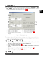
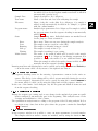
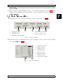
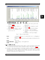
INGOS s.r.o.
AMINO ACID ANALYSER
AAA400
Manual for ChromuLan
PRAGUE
May 4 2001
Producer
:
INGOS
Development
Chemical system
:
:
PiKRON
V. Havlíček - ZMBD chemik
Supplier and service
:
INGOS s.r.o.
K Nouzovu 2090
14316 PRAHA 4
(c) INGOS 2001
Tel: 02/4097683
02/4097692
Fax: 02/4097685
e-mail:[email protected]
www.ingos.cz
INTRODUCTION
CONTROL
ASSESSMENT
TABLE OF CONTENTS
1
2
3
4
1. INTRODUCTION
This is a freely disseminated software serving for controlling the sets of apparatuses
and subsequent assessment of results. The project is initialized and subsidized by
PiKRON whose instruments support communication and control through the uLAN
communication protocol.
At present the system is developed in the DELPHI environment for WINDOWS NT or
WINDOWS 2000 and an extension for LINUX is expected.
This manual deals with the use of the ChromuLan program for the Amino Acid Analyzer
AAA 400. In this case the program uses standard assessment and a special program
module for the control of the Amino Acid Analyzer.
Fig. 1. ChromuLan
The program is structured in such a manner that the entire system can operate in a
fully automatic mode. Set a sequence in the program, within the framework of which
each sample is assigned an analytic program and assessment method. The apparatus
will process samples in an automatic manner, ensures the equilibration of the column
during the passage between analytical programs and will automatically assess the
results according to the method pre-set.
INGOS s.r.o.
Page 4
1
2. CONTROL
The control module for AAA 400 is activated through the function Aplication ) Amino
Acid Analyzer . At the same time when the control module is activated, also the
technological window of the Analyzer will open (fig. 2).
1.
2.
3.
4.
Current puffer number display
Pump 1 pressure display
Pump 2 pressure display
Current sample test tube number
display
5.
6.
7.
8.
Column temperature display
Reactor temperature display
State line, see Chapter 2.5
Control button panel
Fig. 2. Technologické okno
The left part of the technological window contains a chart of the analyzer in which the
status of individual apparatuses is displayed. The lower right part contains buttons
serving for controlling individual functions.
2.1 turning on of the Analyzer
1. Check the apparatus and operation chemicals (see the User’s Manual for AAA
400 and its chapter on the PUTTING INTO OPERATION)
2. Check the setting of parameters (2.2).
3. Turn on the apparatus by using the button On/O situated in the technological
window.
4. Insert samples into the dispensing disk and prepare the sequence (2.4).
5. Wait until the apparatus is ready (2.5).
6. Turn on the sequence by using the Start button.
2.2 Setting
INGOS s.r.o.
Page 5
2
AAA400
Section 2: CONTROL
By pressing the button Setting you will call out the dialog serving for the setting of basic
parameters of the program and starting parameters of the apparatus.
Sequences directory
Directory which contains all sequences.
Programs directory
Directory which contains analytical programs.
Methods directory
Directory which contains assessment methods.
Current Sequence
Current sequence name (2.4).
Default Prog. Name
Name of the program to be set in the heading during the
creation of a new sequence (2.4.1).
Default method for new seq.Name of the method to be set in the heading during the
creation of a new sequence (2.4.1).
P1 Flow [ml/min]
Pump 1 flow rate [0.3].
P1 Press Min [MPa]
Lower limit of the pump 1 pressure [2.0].
P1 Press Max [MPa]
Upper limit of the pump 1 pressure [9.0].
P1 Deviation [%]
Permitted oscillation of the pump 1 pressure [50].
P2 Flow [ml/min]
Pump 2 flow rate [0.2].
P2 Press Min [MPa]
Lower limit of the pump 2 pressure [0.1].
P2 Press Max [MPa]
Upper limit of the pump 2 pressure [3.0].
P2 Deviation [%]
Permitted oscillation of the pump 2 pressure [80].
Column Temp. [C]
Column temperature [60].
Col. Temp. Min Dif [C]
Maximum permitted column temperature drop [5].
Col. Temp. Max Dif [C]
Maximum permitted column temperature increase [5].
Colum Temp. Dev. [%]
Permitted oscillation of the column temperature [10].
React. Temp. [C]
Reactor temperature [121].
React. Temp. Min Dif [C] Maximum permitted reactor temperature drop [5].
React. Temp. Max Dif [C] Maximum permitted reactor temperature increase [5].
React. Temp. Dev. [%]
Permitted oscillation of the reactor temperature [10].
2.3 Analytical program
The analytical program serves for controlling the apparatus during the sample analysis.
Each line of the program defines activities of the apparatus at a given time.
By pressing the Program button in the technological window call out the menu which
has three items:
New
Calls out the window for editing a new program.
Open
Calls out the menu for opening a program.
Edit
Calls out the window for editing the program which was edited during the last session.
The program editing window is in fig. 3. The program lines are automatically arranged
according to the time. Inserting new lines and deleting old lines can be carried out
by using the Insert and Deletekeys or from the menu which can be called out by using
the right mouse button.
With regard to the automatic arrangement of the lines it is possible that at a change
of time the line will move to another position. During modifications being made in
INGOS s.r.o.
Page 6
2
AAA400
Section 2: CONTROL
1. Time
2. Column temperature
3. Puffer number
4. Command
5. Note
Fig. 3. Okno editace programu
a program it is necessary to work with this function carefully and always, after a
change in time, to check whether the right line is being edited.
The following commands may appear in the AA Command column:
Inject
Dispense the sample from the loop. This command should always be
in the time 0.
Zero
Zero the detector. This command should be addressed to the place
for which it is sure that there is a baseline.
StartEquil
From this command the equilibration analysis starts (2.4.2).
H2O
Switch the pump 2 entry to water.
NHD
Switch the pump 2 entry to ninhydrin.
StopAcq
terminates the data record.
Load
Prepares another sample to the loop.
None
No action is being made.
After modification it is necessary to save the program. Saving will be carried out by
using the Save command from the menu which is called out with the help of the right
button. If you are correcting a program while an analysis is running, the changes will
only be applied during the next sample.
2.4 Sequence
INGOS s.r.o.
Page 7
2
AAA400
Section 2: CONTROL
The sequence specifies an arranged set of samples during processing. Each line of the
sequence corresponds to one sample. The sequence is automatically named according
to the date of creation. At the same time when the sequence is created, a directory
of the same name is created on the disk and individual analyses are stored into it.
By pressing the Sequence button in the technological window call out the menu which
has three items:
New
Makes it possible to create a new sequence. Before actual editing it
is necessary to fill the heading of the sequence first (2.4.1).
Open
Calls out the menu for the opening and editing of a sequence which
has already been saved. At the same time it will set this sequence as
the current one.
Edit
Calls out the window for editing the current sequence.
If the sequence is being executed, you will call out directly the editing of the current
sequence. In the sequence being executed it is only possible to change the samples
which are in the ”Waiting” state.
The window for editing the sequence is in fig. 4. Individual columns have the following
meaning:
1
1.
2.
3.
4.
2
3
4
Name of sample
Number of test tube
Sample description
Name of the user who has been
analyzing the sample
5
5.
6.
7.
8.
6
7
8
File name
Analytical program name
Sample processing state
Method name
Fig. 4. Window for editing the sequence
Sample name
Vial Nr.
INGOS s.r.o.
Sample name. If it remains undefined, the file name will be
filled in automatically.
Number of test tubes from which the sample in question will
be taken. It must be filled in. if a sample is added, the numPage 8
2
AAA400
Section 2: CONTROL
ber which follows by the highest number used will be filled in
automatically (greater by 1).
Sample Desc.
Sample description. Not obligatory.
User name
Name of the user who has been analyzing the sample
File name
Name of the file on the disk. It is obligatory, if a sample is
added, it will automatically be filled in as ”Sample”, together
with the ordinal number.
Program name
Analytical program name. It is obligatory. If a sample is added,
the program name from the sequence heading is automatically
added (2.4.1).
State
Sample processing state. Individual states are marked in red
for the purpose of fast orientation.
Error
Error state. There was an error during the sample analysis.
Done
The sample was processed in order (OK).
Running
The sample is currently being processed.
InLoop
The sample is ready in the loop.
Waiting
The sample is waiting for processing.
Method name
The name of the method which will be used for the sample
assessment (3.3). It is obligatory, but during assessment it is
possible to change the method on an additional basis (3.3).
When the sample is added, the method name is filled in automatically from the sequence heading (2.4.1).
Inserting new lines and deleting lines can be carried out by using the Insert and Deletekeys
or from the menu called out by means of the right mouse button.
2.4.1 Sequence heading
The sequence heading serves for the entering of parameters common for the entire sequence. The dialog for its editing will be called out automatically during the creation
of a new sequence, alternatively it can be opened by using the command Header in
the menu, which is called out by using the right button in the sequence window.
In the case of the Amino Acid Analyzer only the Program and Method items are used
from the sequence heading.
2.4.2 Equilibration analysis
During the sequence processing and on any change in the analytical program an equilibration analysis is automatically put on the beginning. This analysis serves for the
cleaning and stabilization of the column.
The equilibration analysis runs according to the program of the following analysis. It does
not begin at zero time, but at the place where the program contains the StartEquil
(2.3) command.
2.4.3 mass assessment
In the sequence window it is possible to carry out mass assessment of several samples.
The samples which we want to assess are marked, and by using the function Show
INGOS s.r.o.
Page 9
2
AAA400
Section 2: CONTROL
result for sel. from the menu under the right mouse button the result window is called
out.
Samples for mass assessment must have the correct method assigned to them (3.3) and a
standard. The standard can be assigned to selected samples by means of a function
Assign calib. le .
2.5 State information
The right part of the technological window contains a state line, see fig. 5.
1. Apparatus state
2. Analysis time
3. Current program name
4. Current sample name
5. Current sample state
Fig. 5. Stavový řádek
Other information concerning the state of the apparatus can be called out by pressing
the button State see fig. 6.
1
2
3
4
5
6
8
1.
2.
3.
4.
5.
6.
7.
8.
Current sequence
Pump 1 state
Pump 2 state
Column state
Reactor state
Dispenser state
Detector state
Absorbance values
7
Fig. 6. State information
INGOS s.r.o.
Page 10
2
3. ASSESSMENT
For AAA400 the assessment with the help of a standard is used. With regard to the fact
that chemistry used in the Analyzer changes in the time (NHD is getting old), it is
necessary to arrange a standard after each 5 to 10 samples.
For the purpose of elimination it is possible to use also an internal standard. It is mainly
used for the elimination of an error arising during the preparation of the sample.
3.1 Assessment procedure
1. Open the analysis of the standard. Press the button Graph in the technological
standard and select a standard.
2. If you did not mark the standard in the sequence, mark it additionally, in the
headings (function Setup) mark the field Cal. Standard.
3. If you did not have in the sequence (2.4) a correctly set method, use the function
Method ) Load From for reading the right method for the standard, see 3.3.3
and activate the function Peak ) Autodetect .
4. Check whether all peaks have been assessed. If not, correct the method, see 3.3.2
and activate the function Peak ) Autodetect .
5. Save the standard File ) Save.
6. Press the button Graph in the technological window and select the analysis which
you want to assess.
7. If you did not have in the sequence (2.4) a correctly set method, use the function
Method ) Load From for reading the right method for the analysis, see 3.3.4 and
activate the function Peak ) Autodetect .
8. Check whether all peaks have been assessed. If not, correct the method, see 3.3.2
and activate the function Peak ) Autodetect .
9. Read the standard of functions Method ) Load Calibration File and activate the
function Peak ) Calculate Amounts .
10. Call out the peak table (fig. 9) Peak ) Browse , where it is possible to check the
results, possibly to print them by using the function Print ) Report.
3.2 Chromatogram window
It is possible to open the chromatogram window in two ways. By pressing the button
Graph in the technological window or from the menu by using the command File )
Open.
You can carry out basic operations with the graph with the help of buttons in the lower
part of the window, see fig. 7. By pressing the button at the same time with the Shift
key you may use the function in question on a repeated basis.
By pressing the right mouse button in this window call out the chromatogram menu
which would have the following items:
Setup
- setting the analysis parameters
Method
- method submenu
Baseline
- baseline submenu
Peaks
- peak submenu
INGOS s.r.o.
Page 11
3
AAA400
Section 3: ASSESSMENT
3
1 2 3 4 5 6
7
8
9
10
1. Button for manual creation of a
baseline (3.2.1)
2. Button for manual creation of
peaks (3.2.1)
3. Button for the setting of a cut-out
4. Button for the returning of the
previous cut-out
5. Button for the cursor position display mode
6. Button for the comparison of analyses, see 3.5
7. Activation of the baseline display
8. Activation of the axes display
9. Activation of the peak description
display
10. Activation of the report display
Fig. 7. Okno chromatogramu
Math
- conversion submenu, to be used in the case of overlapping of
analyses, see 3.5
View
- setting of visible items (axis, peak description, baseline and others)
Scale
- basic scale
Copy to clipboard - graph copying to other applications
Print
- printing
3.2.1 Editing peaks
You can edit peak parameters directly in the graph or in the peak table. In the graph
you can edit also the baseline and the integration marks of the peaks, see fig. 8.
If you want to edit peak parameters in the graph, mark the peak by clicking on the
description and by further clicking on the description call out the dialog for editing
peak parameters. You can change the position of the end points of the baseline and
integration marks directly by using the mouse.
INGOS s.r.o.
Page 12
AAA400
Section 3: ASSESSMENT
1.
2.
3.
4.
5.
1
Peak description
Data measured
Baseline
Baseline end point
Peak integration marks
2
3
3
4
5
Fig. 8. Editace píku
Addition of further peaks and sections of the baseline is carried out with the help of
buttons in the lower part of the chromatogram window (3.2).
Call out the peak table by using the function Peak ) Browse see fig. 9
3.3 Method
The method contains information for the assessment of the analysis. The method forms
a part of any analysis. But it can also be saved in a separate file and to be read again
from this file. This can also be made by using the function Method ) Save To and
Method ) Load From .
In the case of the Amino Acid Analyzer the method set in the sequence is automatically
inserted into the analysis, see 2.4.
The data in the method can be divided into three parts: method heading, peak description
ad baseline description.
3.3.1 Method heading
Call out the method heading by using the function Method ) Edit see fig. 10. The
meaning of individual items is as follows.
Method Template
Name of the file from which the method was created
Calibration File
Name of the standard
Calibration File
Method file name
Duration
This parameter is not used for the time being
Base min. interval
To be used during automatic detection of the baseline, it says
how long the straight section must be so that it can be considered as a baseline.
INGOS s.r.o.
Page 13
AAA400
Section 3: ASSESSMENT
1
2
3
4
5
6
7
8
3
1.
2.
3.
4.
5.
Retention time
Peak area
peak name
amino acid quantity
Coefficient for the computation of
quantity, see 3.3.4 and 3.4
6. Window for the assignment of the
method peaks, see 3.3.2
7. Response, see 3.4
8. Name of the line from which the
peak is assessed. If the field is
empty, it is assessed according to
a green color, while the ”B” letter
means that it is assessed from a
blue color.
Fig. 9. Tabulka píků
Fig. 10. Hlavička metody
Base max. diff
Min. peak height
INGOS s.r.o.
Specifies maximum noise which could appear on the section
which is considered to be the baseline.
Minimum peak height. The peaks which are lower are ignored
during the self-detection.
Page 14
AAA400
Section 3: ASSESSMENT
Min. peak width
Minimum peak width The peaks which are narrower are ignored during the self-detection.
Use negative peaks Mark the field if you want to assess negative peaks. It is not
used in the case of the Amino Acid Analyzer.
Calc Amounts
Mark the field if you want to compute the quantity automatically. In the case of the Amino Acid Analyzer it is always
marked.
Use Calibration File Mark the field if you want to use the standard. In the case of
the Amino Acid Analyzer it is always marked.
Use Internal StandardMark the field if you want to use the internal standard.
Factor
Conversion factor, see 3.4 .
Calibration File Age Date and time for the reading of the calibration file. During
computation it is necessary to check whether the calibration
file was not modified after this date. In the case that it was, it
is necessary to carry out its new reading.
No Unknown Peak If you mark this field, only those peaks are assessed which are
defined in the method in question.
3.3.2 Method peaks
By using the function Method ) Peaks ) Browse you will call out the method peak
table. This table is the same as the peak table. You can add peaks into this table by
using the Insertkey, alternatively you can copy the peaks marked from the analysis
by using the command Peaks ) Copy Selected To Method .
The peaks of the method are assigned to the peaks measured with the help of the retention
time and window. If the peak is not assigned correctly, change the retention time in
the method peak table, or enlarge the window. If the window is changed, be careful
that the windows should not overlap.
3.3.3 Method for the standard
The method for the standard must have in the heading (3.3.1) the following setting:
Faktor=1. Moreover, the method peak table must have in the column Amount the
settings of quantities of individual amino acids in the standard. The column UsrPeakCoef must be 1.
Also Multiply Factor and DivideFactor in the sequence must be set to 1.
3.3.4 Method for the sample
If you want to know the results in grams, you must set molar weights of individual amino
acids in the method peak table in the column UsrPeakCoef.
If you are using a constant base and dilution, include it into Faktoru in the method
heading, if you do not use Multiply Factor and DivideFactor in a sequence.
The name of the peak in the method for the sample and in the method for the standard
must be the same, otherwise the peak in question will not be assessed.
3.4 Computation
INGOS s.r.o.
Page 15
3
AAA400
Section 3: ASSESSMENT
In the case of the Amino Acid Analyzer it is necessary to use always a computation with
the standard. This computation is carried out according to the following formula:
Amount =
M utiplyF actor
Area
U srP eakCoef F actor Response
DivideF actor
where: Area is the peak area, UsrPeakCoef is the coefficient from the peak table. Th
factor is set in the method heading and is the same for all peaks and for all samples
assessed by using the method in question. MutiplyFactor and DivideFactor are set
for each sample separately in a sequence or in the heading of the sample, they are all
for all peaks. Response is computed from the standard according to the formula:
Response =
Areastd
M utiplyF actorstd
U srP eakCoefstd F actorstd Amountstd
DivideF actorstd
The meaning of individual members is the same, they are only taken from the standard.
3.5 Comparison of analyses
The program makes it possible to enter several analyses into a single graph. This can
be made by pressing the button serving for comparison of analyses, see fig. 7 and
then open a subsequent analysis of functions File ) Open. Individual analyses can
be moved and enlarged by using the functions from the submenu Math in the chromatogram menu.
Another possibility of displaying several analyses into a single graph is by using the
function Open selected in one window in the menu which will be called out by using
the right button in the sequence window.
It is possible to switch active analyses by using the function Overlay from the chromatogram menu.
INGOS s.r.o.
Page 16
3
4. TABLE OF CONTENTS
1. INTRODUCTION . . . . . . . . . . . . . . . . . . . . . . . . . . . . . . . . . . . . . . . . . . . . . . . . . . . . . . . . . . . . . 4
2. CONTROL . . . . . . . . . . . . . . . . . . . . . . . . . . . . . . . . . . . . . . . . . . . . . . . . . . . . . . . . . . . . . . . . . . . . 5
2.1 turning on of the Analyzer . . . . . . . . . . . . . . . . . . . . . . . . . . . . . . . . . . . . . . . . . . . . . . . . 5
2.2 Setting . . . . . . . . . . . . . . . . . . . . . . . . . . . . . . . . . . . . . . . . . . . . . . . . . . . . . . . . . . . . . . . . . . . 5
2.3 Analytical program . . . . . . . . . . . . . . . . . . . . . . . . . . . . . . . . . . . . . . . . . . . . . . . . . . . . . . . 6
2.4 Sequence . . . . . . . . . . . . . . . . . . . . . . . . . . . . . . . . . . . . . . . . . . . . . . . . . . . . . . . . . . . . . . . . . 7
2.4.1 Sequence heading . . . . . . . . . . . . . . . . . . . . . . . . . . . . . . . . . . . . . . . . . . . . . . . . . . 9
2.4.2 Equilibration analysis . . . . . . . . . . . . . . . . . . . . . . . . . . . . . . . . . . . . . . . . . . . . . . 9
2.4.3 mass assessment . . . . . . . . . . . . . . . . . . . . . . . . . . . . . . . . . . . . . . . . . . . . . . . . . . . . 9
2.5 State information . . . . . . . . . . . . . . . . . . . . . . . . . . . . . . . . . . . . . . . . . . . . . . . . . . . . . . . . 10
3. ASSESSMENT . . . . . . . . . . . . . . . . . . . . . . . . . . . . . . . . . . . . . . . . . . . . . . . . . . . . . . . . . . . . . . . 11
3.1 Assessment procedure . . . . . . . . . . . . . . . . . . . . . . . . . . . . . . . . . . . . . . . . . . . . . . . . . . . 11
3.2 Chromatogram window . . . . . . . . . . . . . . . . . . . . . . . . . . . . . . . . . . . . . . . . . . . . . . . . . . 11
3.2.1 Editing peaks . . . . . . . . . . . . . . . . . . . . . . . . . . . . . . . . . . . . . . . . . . . . . . . . . . . . . 12
3.3 Method . . . . . . . . . . . . . . . . . . . . . . . . . . . . . . . . . . . . . . . . . . . . . . . . . . . . . . . . . . . . . . . . . 13
3.3.1 Method heading . . . . . . . . . . . . . . . . . . . . . . . . . . . . . . . . . . . . . . . . . . . . . . . . . . . 13
3.3.2 Method peaks . . . . . . . . . . . . . . . . . . . . . . . . . . . . . . . . . . . . . . . . . . . . . . . . . . . . . 15
3.3.3 Method for the standard . . . . . . . . . . . . . . . . . . . . . . . . . . . . . . . . . . . . . . . . . . 15
3.3.4 Method for the sample . . . . . . . . . . . . . . . . . . . . . . . . . . . . . . . . . . . . . . . . . . . . 15
3.4 Computation . . . . . . . . . . . . . . . . . . . . . . . . . . . . . . . . . . . . . . . . . . . . . . . . . . . . . . . . . . . . 15
3.5 Comparison of analyses . . . . . . . . . . . . . . . . . . . . . . . . . . . . . . . . . . . . . . . . . . . . . . . . . . 16
4. TABLE OF CONTENTS . . . . . . . . . . . . . . . . . . . . . . . . . . . . . . . . . . . . . . . . . . . . . . . . . . . . . 17
4.1 List of picturtes and tables . . . . . . . . . . . . . . . . . . . . . . . . . . . . . . . . . . . . . . . . . . . . . . 17
4.1 List of picturtes and tables
Fig. 1. ChromuLan . . . . . . . . . . . . . . . . . . . . . . . . . . . . . . . . . . . . . . . . . . . . . . . . . . . . . . . . . . . . . . . . 4
Fig. 2. Technologické okno . . . . . . . . . . . . . . . . . . . . . . . . . . . . . . . . . . . . . . . . . . . . . . . . . . . . . . . . . 5
Fig. 3. Okno editace programu . . . . . . . . . . . . . . . . . . . . . . . . . . . . . . . . . . . . . . . . . . . . . . . . . . . . . 7
Fig. 4. Window for editing the sequence . . . . . . . . . . . . . . . . . . . . . . . . . . . . . . . . . . . . . . . . . . . . 8
Fig. 5. Stavový řádek . . . . . . . . . . . . . . . . . . . . . . . . . . . . . . . . . . . . . . . . . . . . . . . . . . . . . . . . . . . . . 10
Fig. 6. State information . . . . . . . . . . . . . . . . . . . . . . . . . . . . . . . . . . . . . . . . . . . . . . . . . . . . . . . . . 10
Fig. 7. Okno chromatogramu . . . . . . . . . . . . . . . . . . . . . . . . . . . . . . . . . . . . . . . . . . . . . . . . . . . . . 12
Fig. 8. Editace píku . . . . . . . . . . . . . . . . . . . . . . . . . . . . . . . . . . . . . . . . . . . . . . . . . . . . . . . . . . . . . . 13
Fig. 9. Tabulka píků . . . . . . . . . . . . . . . . . . . . . . . . . . . . . . . . . . . . . . . . . . . . . . . . . . . . . . . . . . . . . . 14
Fig. 10. Hlavička metody . . . . . . . . . . . . . . . . . . . . . . . . . . . . . . . . . . . . . . . . . . . . . . . . . . . . . . . . . 14
INGOS s.r.o.
Page 17
4