Download G. Terreni. The CIFF System: an Overview. Technical Report.

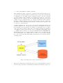
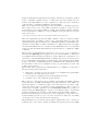
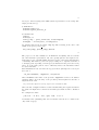
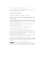
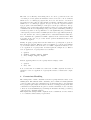
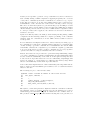
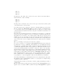
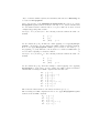
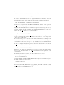
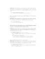
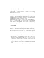
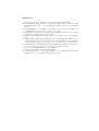
The CIFF System: an Overview
Giacomo Terreni
Dipartimento di Informatica, Università di Pisa
Email: [email protected]
Abstract. This paper details the structure and the main algorithms in
the CIFF System 4.0, a SICStus Prolog implementation of the CIFF
proof procedure.
1
The high-level design of the CIFF System
The CIFF System 4.0 requires SICStus Prolog 3.11.2 (or newer versions of SICStus Prolog 3 release) and it starts by compiling, on the Prolog top-level shell,
the ciff.pl file which, in turn, compiles all the CIFF System modules.
The CIFF System is composed by the following modules:
– the main module1 : it provides the main predicate (run ciff/3) for starting
a CIFF computation and it manages the main computational cycle,
– the flags module: it provides all the CIFF flags an user can set to change the
CIFF behavior (e.g. turning on/off the NAF module, the level of debugging
info returned to the user and so on); all the flags are detailed in the CIFF
manual [8],
– the preprocess module: it provides the translation from the user’s abductive
logic program with constraints to its internal representation,
– the proc module: it provides the predicate sat/2 which, roughly speaking,
implements the CIFF proof rules,
– the proc-aux module: it provides auxiliary predicates to sat/2,
– the aux module: it provides general auxiliary predicates,
– the constraints module: it provides the wrapper around the SICStus CLPFD
constraint solver,
– the debug module: it provides predicates to return debugging info to the
user, and
– the ground-ics module: it provides an efficient algorithm for handling some
classes of integrity constraints (see Section 7).
Once compiled the system, a CIFF computation starts with the run ciff/3
call:2
1
2
Each “module” is implemented in a .pl file having the same name with a ciffprefix. E.g. the ciff-main module is implemented by the ciff-main.pl file
In what follows, we will use several Prolog standard notations: variables names start
with capital letters, ! is the cut operator, [ ] is the notation for lists and \+ stands
for negation. Moreover the notation pred/n stands for “the predicate pred with arity
n” and finally +,- before a predicate argument Arg represent that Arg is an “input”
argument and an “output” argument respectively.
| ?- run_ciff(+ALPFiles,+Query,-Answer).
where ALPFiles is a list of .alp whose conjunction represents an abductive logic
program with constraints (ALPC) and Answer is the output variables which will
be instantiated to the CIFF extracted answers (if any) to the list of literals
provided in Query. The possibility of specifying more than one .alp in the
ALPFiles list is to facilitate the user in writing CIFF applications. A typical
example is a two terms list where one .alp file contains the clauses and the
integrity constraints which specify the problem and the other file contains the
specification of the particular problem instance. In this way the first file could
be reused for others instances.
A CIFF computation is composed by both a preprocessing phase which both
translates ALPFiles into its internal representation and initializes the system
data structures and an abductive processing loop implemented as a recursive
call to the sat/2 predicate. Each call to the sat/2 represents an application
of a CIFF proof rule and at the end of the loop Answer is instantiated either
to a CIFF extracted answer or to the special undefined (if the Dynamic Allowedness rule has been applied). Further answers can be obtained through
Prolog backtracking. If no answer has been found, the system fails returning
the control to the user. The main CIFF computational cycle is described in the
following picture.
Fig. 1. The CIFF System: main computational cycle
The preprocessing phase, detailed in Section 2, stores the iff-definitions derived
from the user program into an internal representation in which the various ele-
ments are maintained in disjoint sets depending on their type: abducibles, defined
atoms, constraints, equalities and so on. The same type-based partition is performed on the first CIFF node of the computation, composed by the conjunction
of the integrity constraints in ALPFiles and the Query.
This node is passed as the first input of the sat(+State, -Answer) predicate,
where State is the state of the CIFF computation, which is composed by the
representation of the current CIFF node plus other auxiliary run-time information, in particular for NAF (see below). A CIFF node is represented by a state
atom of the form:
state(Diseqs,Constraints,Implications,DefinedAtoms,Abducibles,Disjunctions)
where the arguments represent the CIFF conjuncts of the node. They are maintained aggregated, depending on their “type” (and their names are quite selfexplanatory): Diseqs represents the set of CIFF disequalities, Constraints represents the current finite domain constraint store, Implications the set implications, DefinedAtoms the set of defined atoms, Abducibles the set of currently
abduced atoms and finally Disjunctions represents the set of disjunctive CIFF
conjuncts.
Each element in Disjunctions represents a choice point of the computation
and when the Splitting rule is applied on it, the current CIFF node is selected
in a CIFF formula following the left-most criteria. When the computation on a
certain node ends (instantiating Answer or failing), the next node is selected via
Prolog backtracking. Delegating the management of the switching among CIFF
nodes to the Prolog backtracking allows to maintain in the current State only
the information of the selected CIFF node and, for performances, it is the only
possible practical choice.
Each sat/2 clause represents the implementation of a CIFF proof rule and it
has the following general structure:
1. a first part to search for a rule input in the node satisfying the applicability
conditions of the implemented proof rule
2. a second part for applying the rule and updating the State
3. a recursive call to sat/2 with the updated State.
The search for a rule input is done scanning sequentially the CIFF conjuncts
in the current node. Thus, maintaining a type-based partition of the CIFF conjuncts throughout a computation plays a very important role in terms of efficiency and clarity of the code. This is because each CIFF proof rule operates on
certain types of CIFF conjuncts (e.g. the Unfolding atoms rule operates on
defined atoms, the Factoring rule operates over abducibles and so on) and that
separation facilitates the search for a rule input among the CIFF conjuncts.
If such a rule input has been found, the concrete application of the rule is performed (relying upon the procaux, aux and constraints modules, also depending
on the given proof rule), and the State is updated.
Implementing the proof rules as sat/2 clauses, implies that, due to the Prolog
semantics, the order of these clauses determines the priority given by the CIFF
System to a certain proof rule during the computation. Roughly speaking, the
system tries to apply the proof rule implemented in the first sat clause, if no rule
input is found, then the following sat clause is tried. If no rule can be applied
to a node and no inconsistencies have been detected, an abductive Answer is
extracted and then returned to main module.
When all the choice points have been traversed, the CIFF computation ends
returning the answer no to the user indicating that no more answers can be
found.
What described above outlines the implementation of the CIFF selection function. We use a classical Prolog-like selection function, i.e. we always select the
left-most CIFF node in a CIFF formula. It is not a fair selection function in the
sense that it does not ensure completeness (see [6] for further details), but it has
been found as the only possible practical choice in terms of efficiency (in both
time and space) taking advantage of Prolog backtracking.
Concerning the order of selection of the proof rules in a CIFF node, this is
determined by the order of the sat clauses. If a sat clause defining a CIFF proof
rule, e.g. Unfolding atoms (R1), is placed before the sat clause defining, e.g.
Propagation (R3), then the system tries to find a rule input for R1 and if no
such rule input can be found, then the system tries the same for R3 and so on.
Further details on this topic are given in Section 5.
However, some CIFF proof rules, in particular those rules regarding equalities
(Substitution in atoms, Equality rewriting in atoms and so on) and the
most part of the Logical simplification rules, are not implemented each one
as a sat/2 clause. Rather they are “embedded” in the other main CIFF proof
rules, i.e. when a proof rule R, e.g. Unfolding atoms, is applied, the system
first determines all the operations on the equalities and the logical simplifications
“arising” from R and then it performs them immediately. Thus the updated
State is not only derived from the application of R but also from the application
of all the other “embedded” proof rules. This point, as detailed in Section 3,
determines a great enhancement of performances and moreover it allows for a
better readability of a CIFF computation for debugging purposes.
Until now we do not have taken into account the NAF module whose details
will be described in Section 6. Just to have a global picture of the system, the
implementation of the NAF extension, following the specifications given in [6],
can be logically split in two parts: one part which handles the marked integrity
constraints and the production of the prv atoms and the second part,i.e. from
the application of the NAF Switch rule onward, checking the so-far produced
prv atoms avoiding new abductions through the NAF factoring rules.
Whether the NAF extension is activated or not the preprocessing phase changes
accordingly producing marked or non-marked implications in the first node. In
the same way NAF proof rules (implemented again as sat clauses) are taken into
account or not by the system. The NAF extension is activated through a CIFF
flag and it requires a distinct preprocessing for integrity constraints accordingly
to the CIFF¬ specifications.
Moreover the State argument of sat, to embrace the NAF extension is a twoterms structure as follows:
state(Diseqs,Constraints,Implications,DefinedAtoms,Abducibles,Disjunctions):
naf_state(DeltaNAF,NAFSwitch)
where DeltaNAF represents the marking set of a CIFF¬ node and NAFSwitch is
a 1/0 flag indicating whether the NAF Switch rule has been applied or not.
The interactions of the modules in a CIFF computation is displayed in Figure
2.
Fig. 2. The CIFF System: modules interactions
In the rest of the chapter, we detail the main interesting parts of the system
together with the solution adopted, avoiding to describe the CIFF System “lineby-line” from begin to end. We start from the preprocessing phase together with
a description of the user input and the returned answer. Then we describe, in
Section 3 and in Section 4, the management of both variables (in particular
their quantification) and constraints. In Section 5 we discuss about the loop
checking routines in the CIFF System. In Section 6 we describe the issues in the
implementation of the NAF extension and finally in Section 7 we describe the
ground-ics module containing an efficient algorithm for evaluating some classes
of integrity constraints.
2
Input Programs, Preprocessing and Abductive Answers
As said in the previous section, a CIFF run starts with a
run ciff(+ALPFiles,+Query,-Answer)
call where the conjunction of the .alp files in the ALPFiles list represents
the user-defined abductive logic program with constraints.
Each abductive logic program with constraints (ALPC) consists of the following
components, which could be placed in any position in any .alp file:
– Declarations of abducible predicates, using the predicate abducible. For
example an abducible predicate abd with arity 2, is declared via
abducible(abd( , )).
– Clauses, represented as
A :- L1, ..., Ln.
– Integrity constraints, represented as
[L1, ..., Lm] implies [A1, ..., An].
where the left-hand side list represents a conjunction of CIFF literals while
the right-hand side list represents a disjunction of CIFF atoms.
Equality/disequality atoms are defined via =, \== and constraint predicates are
#=, #\=, #<, #>, #=<, #>= together with the domain inclusion predicate in
(e.g. X in 1..100). Finally, negative literals are of the form not(Atom) where
Atom is an ordinary atom.
Example 1. The following is the CIFF System representation of the “grass” Example presented in [5].
% Abducibles:
abducible(sprinkler_was_on).
abducible(rain_last_night).
% Definitions:
grass_is_wet :- rained_last_night.
grass_is_wet :- sprinkler_was_on.
shoes_are_wet :- grass_is_wet.
% ICs:
[rained_last_night] implies [false].
Let assume that the file is named grass.alp. The following is the call to run
CIFF on the query shoes are wet:
run_ciff([grass],[shoes_are_wet],Answer).
2
Example 2. The following is the CIFF System representation of the “lamp” Example presented in [3].
% Abducibles:
abducible(empty(_)).
abducible(power_failure(_)).
% Definitions:
lamp(a).
battery(b,c).
faulty_lamp :- power_failure(X), not(backup(X)).
backup(X) :- battery(X,Y), not(empty(Y)).
Let assume that the file is named lamp.alp. The following is the call to run
CIFF on the query f aulty lamp:
run_ciff([lamp],[faulty_lamp],Answer).
2
The preprocess module translates both ALPFiles and Query and stores them
into their internal representation. We can logically split the user input in two
main parts: a static part (iff-definitions) and a dynamic part (query plus integrity
constraints). The main objectives in preprocessing are to separate elements of
both input parts depending on their types (as discussed in the previous section)
and to store the static part in order to efficiently retrieve the information when
needed at run-time.
Each iff-definition is stored in the Prolog global State (through an assertion) in
the form of
iff_def(+PredName, +Arguments, +Disjuncts)
where PredName is the name of the predicate, Arguments is a list of N distinct
variables (where N is the arity of the predicate) and Disjuncts is the list of
disjuncts in the form
disj(+Constraints,+Equalities,+Diseqs,+Implications,+DefinedAtoms,+Abds)
where the list of Implications is obtained transforming the negative literals in
the clauses in implicative form whose internal representation will be discussed
later.
For example the clause
p(X,Y,d) :- X #> 5, a(Y), q(Z), r(X), Y \== Z
is translated into (assuming that a/1 is abducible and the above clause is the
only clause for p/3):
iff_def(p,[X,Y,W],[disj([X#>5],[W=d],[Y\==Z],[],[q(Z),r(X)],[a(Y)])]).
Suppose now that during the computation, we have to unfold p(2,b,d). To
retrieve the iff-definition of tt p/3 we simply call:
iff_def(p,[2,b,d],-Disjuncts)
where Disjuncts in this case will be:
[disj([2#>5],[d=d],[b\==Z],[],[q(Z),r(2)],[a(b)])]
In this way we have both a direct access to the iff-definitions and a clear separation of the elements by their type in order to update efficiently the current
State when needed.
Integrity constraints, instead, are not stored in the Prolog global state as they,
together with the Query, will represent the first CIFF node of the computation.
However, in the internal representation, their components are again separated
depending on their type as follows:
body(BCons,BEqs,BAts,BAbds) implies head(HCons,HEqs,HDiseqs,HAts,HAbds)
Consider the integrity constraint
[not(c), q(Y), p(X), r(Z), X=Y, X\==Z] implies [false]
Its internal representation (assuming r/1 is abducible) is
body([],[X=Y],[q(Y),p(X)],[r(Z)]) implies head([],[X=Z],[],[c],[])
This is because the preprocessing phase translates the negative elements into
their positive form (including disequalities, transformed into equalities) and put
them into the head, eventually removing false3 .
The implicative form of negative literals in the clauses, e.g. not(p), is as follows.
body([],[],[p],[]) implies head([],[],[],[false],[])
The above representation may seem quite complex, but it allows for maintaining
a type-based separation, thus avoiding many run-time routines of type-checking.
The dynamic part of the input represents the State argument of the sat/2
predicate:
state(Diseqs,Constraints,Implications,DefinedAtoms,Abducibles,Disjunctions)
3
Note that, for now, we do not take into account the NAF extension. When we will
describe the NAF extension we will slightly change this representation because, body
negative literals into the body of a marked integrity constraint have to stay in the
body.
where all the components arise from the various conjuncts in the Query, apart
Implications which is composed of the conjunction of all the preprocessed
integrity constraints and the implicative form of the negative literals in the
Query.
The last remarks of this section are about the form of an abductive Answer.
A CIFF extracted answer is represented by a triple, namely a list of abducible
atoms, a list of CIFF disequalities DE and finally a list of finite domain constraints Γ . The set of equalities E is not returned as the final substitution (in
E) is directly applied by the system.
Abducibles:Disequalities:Constraints:Labels
The Labels component, be discussed in Section 4, contains a consistent assignment (or a labeling) of the constraint variables in Constraints and it is an added
feature of the implementation with respect to CIFF specification.
Example 3. The only CIFF extracted answer of the Example 1 is:
[sprinkler_was_on]:[]:[]:[]
The two answers of the Example 2 are:
A1 =
A2 =
[power_failure(b),empty(c)]:[]:[]:[]
[power_failure(_A)]:[_A\==b]:[]:[]
2
3
Variables Handling
Variables play a fundamental role in both the theory and the implementation
of the CIFF proof procedure. The presence of both existentially quantified and
universally quantified variables is difficult to manage at both levels.
We recall that in a CIFF node, a universal variable U is a variable which occurs
only in an implication which also defines the scope of U , while an existential
variable E is a variable occurring in at least a CIFF conjunct which is not an
implication and the scope of E is the whole CIFF node.
In this section we focus on two issues: checking variable quantification at run-time
and the implementation of the proof rules concerning equalities, i.e. Equality
rewriting and Substitution rules. To simplify the presentation, we refer to
those rules as to equality rules.
The main issue in variable quantification is that existentially quantified variables
may occur inside an implication due to a propagation rule application. The implementation of a CIFF proof rule managing implications must take into account
that a variable can be either existentially or universally quantified, in order to
avoid unintended behaviors. Thus, the CIFF System must know at run-time the
quantification of a variable and moreover, as it is largely required throughout a
CIFF computation, there is the need of an efficient access to this information.
The solution adopted is to associate to existential variables the existential/0
attribute. The mechanism of attributed variables ([4]), i.e., roughly speaking,
“appending” some information (attributes) to a variable, allows for determining
variable quantification in a fast and reliable way through a local access to the
variable itself. The idea is very simple: all the variables occurring outside the
Implications argument of the current State have the existential attributed
associated with; during the application of a CIFF proof rule, the existential
attribute is associated to each variable moving from an implication to outside. In
this way at the end of each CIFF proof rule application, we have two disjoint sets
of variables: the set of existentially quantified variables (with the existential
attribute) and the set of universally quantified variables (without attributes).
As said in Section 1, equality rules are implemented at the end of the other main
proof rules. For example, consider to unfold a CIFF conjunct p(X,Y) in a CIFF
node such that the iff-definition of p/2 is:
iff_def(p, [Arg1,Arg2], [disj([],[Arg1=a,Arg2=b],[],[],[],[])]).
Following the CIFF specifications, unfolding will result into the set of equalities
X=Arg1, Y=Arg2, Arg1=a, Arg2=b.
Successively, this set has to be simplified and propagated to the whole node by
applying a number of “variable” CIFF proof rules. In the CIFF System, instead,
the latter operations are done all-in-one, simplifying locally the set of equalities
resulting from the application of a CIFF proof rule and then propagating the
resulting set of substitutions to the node (in case of existentially quantified
variables) or to the implication (in case of universally quantified variables). In
doing this, the system takes advantage of the underlying Prolog unification as
much as possible.
Following CIFF specifications, equality rules rely upon a slightly modified version of the Martelli-Montanari unification algorithm [7] and the problem in using
Prolog unification is again related to variable quantification: being all the variables existentially quantified, from a Prolog point of view, Martelli-Montanari
conditions on variables quantification cannot be checked by Prolog itself.
Due to this, the implementation of the equality rules relies on:
– Prolog unification for all the equality rules not involving implications: this is
because in that case all the variables are existentially quantified, hence the
Prolog unification is able to manage them;
– an explicit implementation of the Martelli-Montanari algorithm (in the procaux module) otherwise
Addressing equality rules at the end of the other main proof rules brings some
important benefits.
The first one is efficiency. Performing all at once those operations at the end
of a main proof rule grants an immediate and local access to those variables
which need to be unified/propagated and, moreover, the absence of dedicated
sat clauses for those rules avoids searching for suitable equalities in the current
CIFF node to be unified/propagated. To give an idea, in a typical abductive
logic program, each main CIFF proof rule gives out the preconditions to the application of 4-5 equality rules: this would have required a correspondent number
of CIFF iterations. Not surprisingly, this point together with taking advantage
as much as possible of Prolog unification boosts significantly the performances
of the system (execution times of CIFF System 3.0 were approximately halved).
Note also that the use of Prolog unification for existential variables makes useless to maintain the equalities as CIFF conjuncts in the current State. This
is because at the end of a proof rule all the possible substitutions have been
exhaustively applied.
Finally, dropping equality rules from the main sat loop brings also a great enhancement in debugging. This is because for a human eye, even an expert human
eye, it is much easier to follow the trace of a CIFF computation without a “verbose” application of equality rules. Consider again the example above. With a
verbose application of equality rules we would have:
1 - p(X,Y)
2 - X=Arg1, Y=Arg2, Arg1=a, Arg2=b
3 - X=a, Y=Arg2, Arg1=a, Arg2=b
...
Instead, applying all-at-once the equality rules we simply obtain:
1 - p(X,Y)
2 - X=a, Y=b
It is obvious that in a CIFF node with tens of CIFF conjuncts and tens of
variables a “verbose” application of equality rules leads to a untraceable computation!
4
Constraints Handling
The management of CLP constrains is another big implementation issue of the
CIFF System. The SICStus CLP constraint solver for Finite Domains (CLPFD
solver ) is a state-of-the-art constraint solver [2] and its interface to the standard
Prolog engine is quite simple and effective. However, as it happens in general with
constraint solver implementations, given a ceratin constraint store, the only way
to know about its satisfiability is performing an exhaustive checking (or labeling)
of the involved constraint variables.
This implies that during a CIFF computation, the constraint store is not ensured
to be consistent, unless labeling is performed.
Labeling is an expensive operation on big constraint stores, hence it should be
used carefully during a CIFF computation. Applying frequently the constraint
solving rule to exhaustively check the constraint store could not be a good practical solution because if on one side some CIFF branches can be cut if the store
is unsatisfiable, on the other side the overhead due to labeling could be very big.
The choice we did in the system is to perform labeling every N CIFF proof rules
applications, where N is modifiable by the user through a CIFF flag. A further
check is always performed at the very end of a CIFF branch computation, when
no other proof rules can be applied to the current node and before an answer is
returned to the user.
Apart from efficiency issues, the main problem in using labeling during a CIFF
computation is that labeling results in a complete grounding of the constraint
variables, thus, the constraint store in the CIFF extracted answer would be
totally ground.
To solve this issue, the simplest solution is to build, on-the-fly, a working copy of
the constraint store with fresh constraint variables and then to perform labeling
on that working copy. If the constraint store is unsatisfiable the current CIFF
branch fails, otherwise the computation goes on with the original copy. But this
does not work in practice because copying a constraint store is a very expensive
operation in terms of both space and time and it is not reliable.
Instead, the solution we adopted is able to perform labeling maintaining a single
copy of the constraint store by using a backtracking-based algorithm which, when
needed, checks the satisfiability of the CLP store through a labeling and then
it restores the non-ground values via a forced backtracking. Surprisingly, this
is the best solution, to our knowledge, for efficiency and memory usage which
allows both satisfiability checks and non-ground answers.
Now we sketch the implementation of that backtracking-based algorithm. We assume to apply it at the last CIFF step in a branch, before to return an abductive
answer to the user.
The following is a piece of the sat last clause.
%%%Final clause: returns an answer if the solver succeed
S1
sat( State, Answer) :S2
...
S3
!,
S4
(label_flag(0) ; label_flag(1)),
S5
run_time_label(CVars),
S6
make_label_assocs(CVars,0,Assocs),
S7
...
The symbol ; at line S4 represents a disjunction with the “standard” backtracking semantics of Prolog: if label flag(0) succeeds, the disjunction becomes a
backtracking point and label flag(1) is evaluated in case of failure later on.
The predicate label flag represents whether labeling has been performed on
this store (label flag(1) succeeds) or not yet (label flag(0) succeeds). It is
asserted, with value 0, in the Prolog global state at CIFF System initialization
as follows:
assert(label_flag(0)).
The asserted value of label flag is then used in run time label(CVars) which
effectively performs the labeling on the constraint variables CVars. The predicate
in line S6 regards the added component in the implementation of a CIFF abductive answer: the association of a ground solution for the constraint variables
and it will be discussed later on.
The run time label/1 predicate is defined as follows4
L1
L2
L3
L4
L5
L6
L7
L8
L9
L10
L11
L12
L13
L14
L15
L16
L17
run_time_label(CVars) :labeling_mode(Mode),
retract(label_flag(V)),
if (V = 0) {
if (labeling(Mode,CVars)) {
assert_label_list(CVars,0),
assert(label_flag(1)),
!,
fail
} else {
assert(label_flag(0)),
!,
fail
}
} else {
assert(label_flag(0))
}.
Mode in line L2 represents one of the labeling algorithms offered by the SICStus
CLPFD solver [1]. It can be set through the labeling mode CIFF flag.
In line L3 the value V of label flag is checked (recall that in the sat clause
both 0 and 1 are accepted by the system) and the atom is retracted from the
global Prolog state.
If V = 0 (the initial situation), the labeling (line L5) is performed. If it fails, the
label flag(0) is asserted again and run time label fails too. The last assertion
ensures that also sat fails because the disjunction in line S4 fails. Instead if the
labeling succeeds, then label flag(1) is asserted, run time label fails again
but when the control returns, via backtracking, to sat at line S4, it does not
fail due to the presence of label flag(1) in the Prolog global state. Hence
run time label is traversed again, the test at line L4 fails because now the
4
In real Prolog code the if-else statement is represented by the operators -> ;
whose semantics ensures that the second branch is not a backtracking point if the
first branch succeeds. For readability we use an “imperative-like” syntax.
value of V is 1, and, before to succeed, label flag(0) is asserted again in order
to restore the initial situation.
Note that whenever the run time label clause fails, the variables in the constraint store are restored via Prolog backtracking. This happens also when the
labeling succeeds.
In this way, if labeling succeeds, and then label flag(1) is asserted, we are
ensured that the current constraint store is satisfiable but constraint variables
are not bound to ground values.
The assert label list/2 predicate in line L6 simply asserts in the Prolog
global state the numeric values returned by labeling. Those assertions are done
maintaining the positional order of the list of variables CVars and they are used
by the make label assocs to retrieve the consistent assignment to be displayed
to the user together with the abductive answer.
The other use of the algorithm (every N CIFF steps) is very similar. The only
difference is that the assertions of the ground values are not performed and
moreover, in the real code, there is a further flag for distinguishing whether it is
the last step or an N th step.
5
Loop Checking and CIFF Proof Rules Ordering
CIFF specifications do not ensure that a CIFF computation terminates. E.g., a
CIFF computation for the query p with respect to the abductive logic program
composed of the single clause p ← p, will loop forever applying infinitely unfolding. This example (and many other examples) has a theoretical justification: p
is undefined under the three-valued completion semantics thus neither the query
p nor the query ¬ p succeeds, leading to infinite looping.
However, when switching from theory to practice, further non-terminating
sources arise which do not have a theoretical justification. In this section we
address four types of non-termination sources:
–
–
–
–
the order of selection of CIFF nodes in a CIFF formula;
the order of selection of the CIFF proof rules;
the order of selection of CIFF conjuncts in a CIFF node;
CIFF proof rules which cannot be applied twice in a CIFF branch.
Both in the specifications and in the implementation, the number of leaf CIFF
nodes in a CIFF formula can be incremented only by the application of Splitting on a disjunctive CIFF conjuncts. While, theoretically, any leaf node can be
selected at any CIFF step, in the system we implemented the left-most strategy. This implies that, sometimes, abductive answers can never be returned to
the user because the system loops forever in a non-terminating branch. This
choice follows the classical Prolog approach and it allows for using directly the
underlying Prolog backtracking in case of failures. The benefits are in terms
of efficiency and simplicity because no additional machinery is needed to keep
trace of non-selected nodes, while the main drawback is obviously the potential non-termination. However, we argue that managing even small-medium size
CIFF applications, this approach is the only computationally feasible approach
because managing branching without relying upon Prolog backtracking is computationally very expensive in both time and space.
The second source of non-termination is the order of selection of the CIFF proof
rules. Consider the abductive logic program composed of the clause p ← p and
the integrity constraint a → f alse where a is an abducible predicate. A CIFF
computation with the query p, a will loop forever if Unfolding atoms has a
higher priority than Propagation. In this case the system applies infinitely
many times Unfolding atoms on p while propagating a to a → f alse, would
lead to an immediate failure.
This is a main issue in implementing CIFF because in general there is no evidence
of which rule has to be applied at each time in order to avoid non-termination,
or at least to reduce the final size of a proof tree. Above the right choice was
Propagation and it seems that setting a high priority to Propagation rule can
prevent some non-terminating situations. However, in general Propagation is a
computationally expensive rule because it increments the set of implications in
a node which are a main source of inefficiency due to the presence of universally
quantified variables. Hence, in many applications it could be better to give a
lower priority to Propagation and in general to rules managing implications.
As we said in Section 1 each CIFF proof rule is implemented as a sat/2 clause
in the proc module. This was a central choice in the design of CIFF and that
solution implies that each proof rule has a predefined priority during a CIFF
computation and it corresponds to its order among the sat clauses. I.e. the
system, at each iteration, tries to apply the proof rule represented by the first
sat clause. If no rule input can be found in the node, the second sat clause is
explored and so on. The last sat clause represent the fact that no rule can be
applied on the node and then an abductive answer is returned to the user.
It is clear that in certain cases, if the order of the sat clauses is “wrong”,
this solution does not prevent non-termination. Nevertheless we think that this
is a good practical solution because on one side it allows to have a modular
implementation of the proof rules and on the other side it is possible to change
the order of the rules simply moving up and down the sat clauses in the proc
module, thus allowing for a simple domain dependent tuning of the system.
The third potential non-termination source is the order of selection of CIFF conjuncts in a node. Consider an abductive logic program composed of the clauses
p ← p and q ← f alse. The query p, q may not terminate Unfolding atoms p
forever. However, if CIFF unfolds q, the query fails immediately. Note that the
CIFF proof rule is the same but in one case CIFF does not terminate and in the
other case it does.
To prevent such behavior, the CIFF System implements a left-most selection
strategy on the lists of typed CIFF conjuncts, but the insertion of new conjuncts
is done at the end of the lists. Consider again the above example and let suppose
to have, in the current State the list [p, q] of defined atoms. First CIFF selects
p as the rule input for Unfolding atoms because is the first element in the list.
The application of the rule will result in inserting again p in the list, but this is
done at the end of the list. Thus the new list of defined atoms will be [q, p].
At the next CIFF step, q will be selected to be unfolded, thus leading to failure.
We believe that this strategy represent a good compromise between efficiency
and loop prevention.
The fourth and last source of non-termination is represented by those CIFF
proof rules which require an explicit loop-checking in the specification of a CIFF
derivation, i.e. Factoring and Propagation5 .
We first consider Factoring. To implement loop-checking for Factoring we
added two numbers to each abducible CIFF conjunct in the current State: a
unique identifier and a factoring counter. I.e. each element in the Abducibles
argument of state is of the form:
Abd:Id:FactCounter
where Id is a unique system-generated integer while FactCounter indicates the
least abducible Abd’ (i.e. the abducible with the least identifier) such that Abd
and Abd’ have not been factorized yet. The list of abducibles is maintained
ordered with respect to the identifiers throughout the computation and when a
new abducible is inserted in the list, its FactCounter is initialized to 1
When Factoring is selected, the system selects a pivot abducible atom
Abd:Id:FactCounter which is the abducible with the least Id such that
FactCounter < Id. If no pivot is found then all the pairs of abducibles have
already been factorized. Otherwise, if Abd is found then the least abducible
Abd’:Id’:FactCounter’ such that FactCounter <= Id’ < Id is searched for.
If there is such an Abd’, then Abd and Abd’ are factorized and FactCounter is
set to Id’ else FactCounter is set to Id + 1 and the next pivot is selected for
Factoring.
Example 4. Consider the following three abducibles in the current State and
let us assume that no Factoring rule has been applied yet in the branch
(FactCounter is set to 1 for all the abducibles):
a(X):1:1
a(Y):2:1
a(Z):3:1
When Factoring is selected for the first time, a(X) is not selected as a pivot
because 1 = 1. Instead a(Y) is selected and it is factorized to a(X). This is
because 1 <= 1 < 2. Then the FactCounter of a(Y) is set to 1 + 1 = 2. We
obtain:
5
Note that in CIFF specifications, also other rules concerning equalities need loopchecking. This is obtained “for-free” in the implementation by performing them at
the end of the other proof rules.
a(X):1:1
a(Y):2:2
a(Z):3:1
At this stage only a(Z) can be selected as a pivot and it is factorized first to
a(X) and then to a(Y) obtaining:
a(X):1:1
a(Y):2:2
a(Z):3:3
At this point no abducible can be selected as a pivot and, indeed, all the pairs
of abducibles have been factorized.
Note that, given a pivot abducible, only those elements which precede it in the
list are considered for Factoring. This is because each pair of abducibles have
to be factorized only once in a CIFF branch. If for each pivot we have would
considered all the abducibles in the list, each pair of abducibles would have been
factorized twice.
Following the specifications, when two abducibles are factorized, e.g. a(X) and
a(Y), in one successor CIFF node the two abducibles are still in the list and the
disequality X ¯
= Y is added to the current State, while in the other successor
CIFF node, the pivot abducible is deleted from the list and the substitution Y
= X is applied to the whole State. If the two abducibles are both ground, then
only one successor node is computed and if they are equal, the pivot is simply
deleted.
The loop checking for propagation is a bit more complex.
In order to perform a loop checking for Propagation which follows exactly the
specifications, we need to maintain a data structure, for each implication in the
current State, containing all the CIFF conjuncts (abducibles and defined atoms)
to which that implication has been propagated to. This data structure can be
very big and checking whether an element occurs in it could be very expensive,
and the situation is worsened by the presence of existentially quantified variables.
Suppose to have a CIFF conjunct p(X) in the State and the clause p(X) ← p(Y )
in the input program which, when applied by Unfolding atoms, introduces a
fresh existential variable in the node. I.e. the atom p(X) is unfolded to p(X1),
then to p(X2) and so on. Each implication containing p(Z) in its body, has to
be propagated to each atom p(Xi) because the Xi variables are all distinct.
Obviously, maintaining for each implication in a node, that structure and checking against it each potential CIFF conjunct to be propagated to, implies a huge
overhead in terms of efficiency.
Our implemented solution avoids such overhead, paying something in terms of
completeness.
The two main ideas are that (1) in most practical cases, Propagation can be
applied only to abducible CIFF conjuncts and (2) if Propagation is applied
only to abducible CIFF conjuncts, the machinery introduced for Factoring can
be reused for Propagation.
Due to the presence of the Unfolding in implications rule, if we do not apply
Propagation against defined atoms, we can only “loose” failure branches, but
not successful abductive answers. We do not prove this but we show several
examples supporting that evidence.
Example 5. Let hP, A, ICi< be the following abductive framework with constraints:
P :
p←p
A:
{a}
IC : [IC1]
p→a
Let us consider the goal p. In this case, either applying or not applying Propagation to [IC1] and p does not change the CIFF computed abductive answers.
If we do not apply Propagation, CIFF loops forever due to the clause p ← p.
Propagating p to [IC1] will lead to the abduction of a. However CIFF still loops
forever, thus computing no abductive answer.
2
Example 6. Let hP, A, ICi< be the following abductive framework with constraints:
P :
A:
IC :
p←b
{a, b}
[IC2]
p→a
Let us consider the goal p. As in the example 5, either applying or not applying
Propagation to [IC1] and p does not change the CIFF computed abductive
answers. The following is a CIFF computation in the first case:
F0
F1
F2
F3
F4
F5
F6
F7
:
:
:
:
:
:
:
:
p,
p,
p,
b,
b,
b,
b,
b,
[p → a]
[p → a], [> → a]
[p → a], a
[p → a], a
[b → a], a
[b → a], a, [> → a]
[b → a], a, a
[b → a], a
The abductive answer that we can extract from F7 is h{a, b}, ®i.
The following is a CIFF computation if we do not apply Propagation against
defined atoms as CIFF conjuncts.
F0
F1
F2
F3
F4
:
:
:
:
:
p,
b,
b,
b,
b,
[p → a]
[p → a]
[b → a]
[b → a], [> → a]
[b → a], a
The abductive answer that we can extract from F4 is again h{a, b}, ®i. As we
can see, not only the answer is the same as in the first case, but the latter
computation is less expensive than the previous one, in terms of number of
steps.
2
It is quite clear that, as exemplified above, the presence of the Unfolding in implications rule makes Propagation against defined atoms redundant in most
cases. The only cases in which this is not true are shown by the following example.
Example 7. Let hP, A, ICi< be the following abductive framework with constraints:
P :
A:
IC :
p←p
®
[IC2]
p → f alse
Let us consider the goal p. In this case, if we apply Propagation to [IC1] and p,
CIFF fails immediately. If we do not apply Propagation, instead, CIFF loops
forever due to the clause p ← p.
2
If we do not apply Propagation against defined atoms, we “loose” above type
of failures. Nevertheless the system benefits of huge efficiency enhancements
because as we will see we can avoid the maintenance of a Propagation data
structure for each implication in a node and this is a great value for most practical
cases. Moreover we argue that most of the “lost” failure answers derive from “illdefined” abductive logic programs (as in the case of the above example), which
should be avoided.
Propagating only abducible CIFF conjuncts, allows to build an efficient loop
checking algorithm similar to the one for Factoring.
Each implication in the tt Implications list of the current State is of the form:
Implication:Id:PropCounter
where Id is a unique system-generated integer while PropCounter indicates the
least item Abd in the Abducibles list such that Abd has not been propagated to
Implication yet.
The added information is used in the same way as for Factoring but some notes
are needed.
Let BAbds the list of abducible atoms in the body of an implication. Only the
first element of BAbds is considered for Propagation. This is an important
computational enhancement and it is a “safe” optimization in the sense that no
potential abductive answers may be lost. Consider, e.g., an implication of the
form:
a1, a2 → head
where a1 and a2 are abducibles. In order to empty the body, thus firing head
as a CIFF conjunct in the node, both abducibles have to be eliminated and this
can be done only by propagating them. It is obvious that not only the order in
which they are propagated is meaningless in this respect, but if Propagation
is applied to all the abducibles, it results in more CIFF steps and thus higher
computational costs. In the above example, if we would apply Propagation
exhaustively we would obtain the following set of implications:
a1, a2 → head
a1 → head
a2 → head
> → head
> → head
thus, potentially, head is fired twice in a CIFF branch. If instead we apply
Propagation only to the first abducible we obtain:
a1, a2 → head
a2 → head
> → head
In this way, the computation is forced to produce a minimal set of implications
firing head only once.
The PropNumber element is initialized to 1 for each Implication and an empty
BAbds are skipped by the loop checking algorithm, thus leaving PropNumber to
1. Each time a Propagation is performed the newly generated implication has
again PropNumber set to 1 because the first abducible is removed by Propagation itself and the new first element of BAbds can be potentially propagated to
the whole set of abducible CIFF conjuncts. When Unfolding in implication
is performed, instead, the newly generated implications have their PropNumber’
element set to the value of PropNumber because the new abducibles in the body
(if any) are put at the tail of BAbds, thus leaving unchanged the first abducible
atom.
The last note concerns the behavior of the system against two identical abducible
CIFF conjuncts in a node. Suppose to have an implication of the form a → h and
two abducible atoms a and a in the current node. The loop checking algorithm
for Propagation does not detect that the two abducibles are identical, thus
opening the door for potential loops. To avoid this, there are two solutions.
The first one is to maintain a Propagation data structure for each implication
recording the abducibles which have been propagated to that implication. But
we want to avoid it. The second one is very simple: give a higher priority to
the Factoring rule than to the Propagation rule. Due to the behavior of
the Factoring, after that Factoring has been applied exhaustively to a node,
it is ensured that no abducible CIFF conjunct can occur twice. Then, simply
moving up the sat clause for Factoring all potential loops for Propagation
are avoided.
6
The CIFF¬ proof procedure
Until now, we have not taken into account the NAF extension apart from a little
overview in Section 1. The implementation of the NAF extension, which can be
activated through a CIFF flag, has been done trying to be as much modular
as possible but, nevertheless, it requires additional routines and data structures
both in the preprocessing phase and in the abductive phase. We “hidden” them
in the previous sections to clarify the presentation of the system as the added
machinery does not affect the guidelines of what discussed before.
Implementing the CIFF¬ proof procedure requires to handle the following three
main issues:
– marked integrity constraints in the preprocessing phase
– new CIFF¬ proof rules
– labeling of a CIFF¬ node after the application of NAF Switch
The addition of new CIFF¬ proof rules reflects in adding new sat clauses: we do
not focus on this point as their implementation is the same as any other CIFF
proof rule.
More interesting is the preprocessing phase where some changes in the representation of integrity constraints are needed, which in turn change the representation of the implications in the current State. To address the CIFF¬ specifications, each integrity constraint (and thus each implication) needs a further
Mark field indicating if it is marked (Mark = 1) or it is unmarked (Mark = 0).
Moreover, Negation rewriting is never applied to a marked implication, hence
negative literals in their bodies are never moved into the head, requiring a further field Negs for their storage. The final representation of an implication in
the CIFF System is the following:
body(BCons,BEqs,BAts,BAbds,BNegs) implies
head(HCons,HEqs,HDiseqs,HAts,HAbds,Mark).
Note that if the NAF extension is not activated, the Mark field is set to 0 and
the BNegs is empty for each implication throughout the computation.
Whenever no other proof rules can be applied to a node the NAF Switch rule
is applied and the node is marked with the current set of Abducibles in the
state. Roughly speaking the current Abducibles have to be “frozen” in order to
be retrieved by the next CIFF¬ step, in particular in the application of NAF
factoring rules.
Rather than adding a new fixed component in the current State, the NAF
Switch rule starts a new preprocessing phase, building an iff-definition for each
abducible predicate considering each abducible CIFF conjunct as a clause for the
corresponding predicate. For example, if a(1), a(2) are all the abducible CIFF
conjunct for a/1, then the iff-definition for a would be:
a(X) ↔ X = 1 ∨ X = 2
.
Instead, if no atom has been abduced so far for a/1, then we would obtain:
a(X) ↔ ⊥
.
In order to distinguish between the original iff-definitions and these ones, the
new iff-definitions are asserted through the predicate naf def/3 as follows:
naf_def(+PredName, +Arguments, +Disjuncts).
Whenever the system starts the NAF Switch rule, all the all the previous
naf def assertions (if any) are retracted.
Asserting new iff-definitions for abducibles, however, requires a big care due to
the presence of existential variables. Consider again the abducible predicate a/1
and suppose that a(1), a(Y ) (with Y existentially quantified) have been abduced
so far. The naf def atom to be asserted would be:
naf_def(a, [X], [[1],[Y]]).
The problem is that when the naf def atom is asserted, the binding to Y is lost,
but we need exactly that variable Y because it can be shared to other components
of the current CIFF node.
The solution adopted is to skolemise the existential variables occurring in the
abduced atoms and then to assert the skolemised abducibles maintaining in the
current State the skolem bindings, i.e. the bindings between existential variables and skolem constants for performing a deskolemisation when needed. In
the above example, the system generates a skolem constant sk 1 for Y and the
naf def atom becomes:
naf_def(a, [X], [[1],[sk_1]]).
Being sk 1 a ground term, nothing is lost. To restore the right existential variable
when needed, the association Y = sk 1 is maintained as an argument of the
current State.
Recall that, as said in Section 1, the current State is of the form:
state(Diseqs,Constraints,Implications,DefinedAtoms,Abducibles,Disjunctions):
naf_state(DeltaNAF,NAFSwitch)
and that the naf state(DeltaNAF,NAFSwitch) component is initialized (also if
the NAF extension is activated) to:
naf_state([],0).
Summarizing, the application of the NAF Switch rule changes
naf state(DeltaNAF,NAFSwitch) by populating DeltaNAF of all the skolem
bindings and by setting NAFSwitch to 1.
In this way in the next CIFF¬ steps, the system is aware of the fact that NAF
Switch has been applied and all the information about the frozen abducibles
can be easily retrieved.
Indeed the cost of retrieving a naf def atom (plus, eventually, deskolemising
non-ground terms) is much cheaper than maintaining a flat data-structure containing all the frozen abducibles throughout the computation and then traversing
it to check whether it contains a certain abducible atom or not.
In particular, maintaining in the global Prolog state the set of frozen abducibles
simplifies the application of the NAF factoring rules which are implemented
in a similar way of Unfolding atoms. We explain this by a simple example.
Suppose to have the set of frozen abducibles a(1), a(Y ) for the predicate a/1. In
this case, the NAF Switch rule asserts the following naf def atom:
naf_def(a, [X], [[1],[sk_1]])
and the skolem binding Y = sk 1 is maintained in the State. Suppose now
that the new abducible a(X) occurs in the current node with X existentially
quantified. The NAF Factoring rules would produce a disjunction of the form
X =1∨X =Y
But the same disjunction is produced by unfolding a(X) with the new iffdefinition plus a deskolemisation step through the equality Y = sk 1. This is
exactly what the NAF factoring rules do.
7
Ground Integrity Constraints
Much work has been done in order to reach an acceptable level of efficiency.
However, the main source of inefficiency in a CIFF computation is probably
represented by the set of implications in a CIFF node. As each implication
has to be checked against each instance of each universally quantified variable
occurring in it, increasing the number of implications in an node pulls down
performances dramatically.
Example 8. Let us consider the following abductive framework hP, A, ICi which
simply represents a graph specification:
P :
A:
IC :
vertex(v1)
vertex(v2)
vertex(v3)
edge(v1, v2)
edge(v2, v3)
®
edge(X, Y ) → vertex(X)
edge(X, Y ) → vertex(Y )
It is straightforward to see that the instances of both integrity constraints will
be ground. More precisely, through the exhaustive application of Unfolding in
implication rule, we will obtain the following set of implications:
(X
(X
(X
(X
= v1, Y
= v2, Y
= v1, Y
= v2, Y
= v2) → vertex(X)
= v3) → vertex(X)
= v2) → vertex(Y )
= v3) → vertex(Y ).
Then the application of other proof rules managing equalities will eliminate
variables making the next implications totally ground:
> → vertex(v1)
> → vertex(v2)
> → vertex(v2)
> → vertex(v3).
In this case there are only four implications, but what about if the graph was
composed of hundreds of edges? We would get thousands of implications in a
node, heavily pulling down performances. Even worst, the above example is really
simple because the implications will be eliminated from a CIFF node. But what
about if an abducible occurred in the body of the original integrity constraint?
Potentially, the derived set of instantiated implications is maintained all along
a CIFF branch due to the presence of the abducible.
2
To (partially) deal with this problem, we introduce a dedicated algorithm for
managing efficiently some classes of integrity constraints (and, in turn, the instantiated implications).
The idea is that in the above example and in many other cases the integrity
constraints are such that:
– the defined atoms in their bodies are not recursive, i.e. their iff-definitions
do not generate a loop and
– the implications (or at least the most part of them) deriving from the integrity constraints via unfolding will be ground.
The first observation allows for thinking about a pre-compilation of the bodies of
the integrity constraints because all the possible unfolding operations are finite
and they could be determined statically. The second observation, i.e. that the
implications become ground implications allows for thinking about an algorithm
which asserts and checks them in the Prolog global state instead of maintaining
them in a CIFF node. If a ground body is satisfied, the relative ground instance
of the head will be put into the CIFF node as a CIFF conjunct.
We define formally the class of predicates which can occur in the body of an
integrity constraint to be a ground one, and then we sketch the algorithm on
simple examples.
We start defining the class of ground extensional predicates.
Definition 1. Let hP, A, ICi< be an abductive logic program with constraints.
We say that a non-equality and non-constraint predicate p with a certain arity
n in the language of hP, A, ICi< is a ground extensional predicate if and only if
it is
– it is a non-abducible predicate and
– it is defined in P by a (possibly empty) set of ground facts.
2
The second definition concerns predicates whose definitions do not depend from
other predicates.
Definition 2. Let hP, A, ICi< be an abductive logic program with constraints.
We say that a non-equality and non-constraint predicate p with a certain arity
n in the language of hP, A, ICi< is a final safe predicate if and only if
– it is an abducible predicate or
– it is a ground extensional predicate.
2
The next class of predicates is the 1-step safe class. The main idea is that
no variable could cause floundering and that a predicate neither is a recursive
predicate nor it depends from another recursive predicate.
Definition 3. Let hP, A, ICi< be an abductive logic program with constraints
and let GDP the dependency graph of P . We say that a non-equality and nonconstraint predicate p with a certain arity n in the language of hP, A, ICi< is a
1-step safe predicate if and only if
– it is a final safe predicate or
– each clause C = p(t1 , . . . , tn ) ← B in P is such that
• for each defined predicate q in B, q does not belong to a loop in GDP ,
and
• for each variable X occurring in C,
∗ X occurs also in an equality atom X = c with c ground or
∗ X occurs also in a non-equality, non-constraint atom in B
2
We are ready to introduce the class of safe predicates.
Definition 4. Let hP, A, ICi< be an abductive logic program with constraints.
We say that a non-equality and non-constraint predicate p with a certain arity
n in the language of hP, A, ICi< is a safe predicate if and only if
– it is a 1-step safe predicate and
– each clause C = p(t1 , . . . , tn ) ← B in P is such that each defined predicate
q in B is a 1-step safe predicate.
We say that an atom is a safe atom if its predicate is a safe predicate.
2
Finally, we define the syntactical conditions for which an integrity constraint is
a ground one.
Definition 5. Let hP, A, ICi< be an abductive logic program with constraints.
An integrity constraint I in IC is a ground integrity constraints if and only if
– each atom occurring in its body is a safe atom and
– each variable X occurring in I, occurs also in a safe atom in its body.
2
The above syntactical conditions are automatically checked by the system which
decides whether an integrity constraint is a ground one or not.
Now we briefly sketch the algorithm itself. The basic idea of the algorithm is
to assert incrementally in the Prolog global state all the partial instances of the
implications derived from ground integrity constraints.
At preprocessing-time, all the partial instances which can be built through the
grounding of the ground extensional atoms are asserted. If for some of such
instances the body is satisfied, the relative head is added to the query.
In Example 8, the two ground integrity constraints can be instantiated at preprocessing time through the grounding of edge(X, Y ), adding to the query the
set
vertex(v1), vertex(v2), vertex(v3).
However, the most interesting part of the algorithm is in the presence of an
abducible atom in the body of a ground integrity constraint. The idea is to
check, after each application of a CIFF proof rule, if a new ground abducible
Abd has been added to the current CIFF node. If it is the case, Abd is matched
against all the partial instances asserted so far in the current CIFF branch, and
then asserting all the new (partial) instances obtained through Abd.
Example 9. Let us consider the following ground integrity constraint:
[ext(X),abd_1(X,Y),abd_2(Y)] implies [false]
where abd 1/2, abd 2/1 are abducibles and ext/1 is defined as follows:
ext(1)
ext(2).
At preprocessing time the system asserts the following partial instances of the
ground integrity constraint:
[abd_1(1,Y),abd_2(Y)] implies [false]
[abd_1(2,Y),abd_2(Y)] implies [false]
taking into account the iff-definition of ext/1. If during the computation,
abd 1(1,4) is abduced then it is matched with all the instances obtaining the
new set of instances:
[abd_1(1,Y),abd_2(Y)] implies [false]
[abd_1(2,Y),abd_2(Y)] implies [false]
[abd_2(4)] implies [false]
Now if abd 2(3) is abduced, the new set of instances becomes:
[abd_1(1,Y),abd_2(Y)] implies [false]
[abd_1(2,Y),abd_2(Y)] implies [false]
[abd_2(4)] implies [false]
[abd_1(1,3)] implies [false]
[abd_1(2,3)] implies [false]
Finally if abd 2(4) is abduced, then we obtain
[abd_1(1,Y),abd_2(Y)] implies [false]
[abd_1(2,Y),abd_2(Y)] implies [false]
[abd_2(4)] implies [false]
[abd_1(1,3)] implies [false]
[abd_1(2,3)] implies [false]
[abd_1(1,4)] implies [false]
[abd_1(2,4)] implies [false]
[] implies [false]
At this stage, false is added to the current CIFF node, thus failing this branch.
2
The only problem is that, while for the extensional ground atoms we are sure
that all the instances will be ground (due to their iff-definition), we cannot say
the same for abducibles.
To address this point, the solution we adopted is the following: when no other
CIFF proof rules can be applied to the node, if there are some non-ground
abducibles as CIFF conjuncts, they are matched against all the partial instances
asserted in the branch. The so obtained instances are inserted in the CIFF node
and then handled by ordinary CIFF proof rules.
Example 10. Consider again Example 9 and let us assume that no CIFF proof
rule can be applied to a node, an abducible abd 2(Z) (Z existentially quantified)
is in the node and the partial instances asserted are:
[abd_1(1,Y),abd_2(Y)] implies [false]
[abd_1(2,Y),abd_2(Y)] implies [false]
[abd_2(4)] implies [false]
In this case, in the CIFF node will be inserted the following implications:
[abd_1(1,Y),Z=Y] implies [false]
[abd_1(2,Y),Z=Y] implies [false]
[Z=4] implies [false]
Roughly speaking, to obtain the instances to be added to the node, we apply
exhaustively a propagation step.
2
In order to check efficiently at every CIFF proof rule application, if an abducible
has been grounded, a further element GroundAbds is added to the state term
of the current State, containing the current set of non-ground abducibles in
the node. If an abducible becomes ground it is matched to the asserted partial instances of the ground integrity constraints and then it is removed from
GroundAbds. When no other CIFF proof rules can be applied, the elements in
GroundAbds are the remaining non-ground abducibles.
Handling at Prolog global state the ground integrity constraints allows for a
huge boost to performances. The decision whether to use or not this algorithm
is left to the user through a CIFF flag, but however, the only case in which it
should not be used is for debugging. I.e. when the user want to keep track step
by step of the CIFF proof rules over the implications.
8
Conclusions
The CIFF System, a SICStus Prolog implementation of the CIFF proof procedure [6], is a state-of-the-art abductive system. Compared with other related
existing tools, it shows unique features (like negation as failure and handling of
variables) and it is directly comparable in performances, as pointed out in [6].
There are, however, several lines for future work. We argue that the main issue
of the CIFF System 4.0 is the lack of a Graphical User Interface (GUI) which
would hugely improve its usability: we hope to add it in the next CIFF System
5 release.
Other interesting features which are planned to be added to the CIFF System 5
release, are the following.
– Full compatibility to the SICStus Prolog 4 release (which is claimed to be
much faster: a porting of the system will benefit at once of this boost in performances) and to SWI-Prolog [9], an interesting open-source Prolog platform.
– The possibility of invoking Prolog platform functions directly. We think that
this would enhance performances and ease-of-programming in CIFF. However, some work has to be done in order to understand how to integrate them
safely.
– Further improvements in the management of ground integrity constraints.
References
[1] SICStus Prolog. http://www.sics.se/isl/sicstuswww/site/index.html.
[2] A. J. Fernández and P. M. Hill. A comparative study of eight constraint programming languages over the boolean and finite domains. Constraints, 5(3):275–301,
2000.
[3] T. H. Fung and R. A. Kowalski. The IFF proof procedure for abductive logic
programming. J. Log. Program., 33(2):151–165, 1997.
[4] C. Holzbaur. Metastructures versus attributed variables in the context of extensible
unification. In PLILP, pages 260–268, 1992.
[5] A. Kakas, R. Kowalski, and F. Toni. The role of abduction in logic programming,
1998.
[6] P. Mancarella, G. Terreni, F. Sadri, F. Toni, and U. Endriss. The CIFF proof procedure for abductive logic programming with constraints: Theory, implementation
and experiments. Theory and Practice of Logic Programming, submitted, 2008.
[7] A. Martelli and U. Montanari. An efficient unification algorithm. ACM Transactions on Programming Languages and Systems, 4(2):258–282, 1982.
[8] G. Terreni. The CIFF System 4.0: User manual.
.
http://www.di.unipi.it/∼terreni/research.php.
[9] J. Wielemaker. An overview of the SWI-Prolog programming environment. In
WLPE, pages 1–16, 2003. http://www.swi-prolog.org/.