
1
SPECTRON
USER MANUAL
V.2
Developers:
Darius Abramavicius
Cyril Falvo
Previous developers:
Wei Zhuang
Ben Robinson
Ravindra Venkatramani
Thomas LaCour Jansen
Zhenyu Li
Eleftheria Kavousanaki
Benoit Palmieri
Tomoyuki Hayashi
Contributors: Benjamin Bulheller
Our team proudly presents SPECTRON version 2.8.x . It is the bug-fix update to
the 2.7 version of SPECTRON. The number of changes from version 1.x.x includes:
the kernel of the code has been completely rewritten, model excitonic systems
were added. A lot of code can been optimized, numerous bugs have been fixed, a
lot of work have been invested into stability. Concepts of input units and different
types of density matrix dynamics were added in 2.7.x
SPECTRON team:
Principal investigator
Prof. Shaul Mukamel
Funding:
National Institute of Health,
National Science Foundation,
US Department of Energy
Primary developers:
Darius Abramavicius:
(initiator)
2003 -- 2010
Wei Zhuang:
(vibrations of proteins)
2004 -- 2008
Cyril Falvo:
(vibrational excitons)
2007 -- 2009
Contributors:
Daniel Healion
2006 – up to now
(website and computer services)
Benjamin Bulheller
2009
(DichroCalc library: UV of peptides)
Benoit Palmieri
(Lidblad theory)
2007 – 2008
Zhenyu Li
(UV of peptides)
2007 – 2008
Eleftheria Kavousanaki
(semiconductor excitons)
2007 – 2008
Tomoyuki Hayashi
(vibrational amide maps)
2003 – 2007
František Šanda
2004 – 2007
(stochastic Liouville equations)
Ben Robinson:
(user interface)
2005 – 2006
2
Ravindra Venkatramani
2003 – 2004
(sum-over-states CGF correlations)
Thomas LaCour Jansen
2003 – 2004
(stochastic Liouville equations)
3
Contents
1 History and present state....................................................................................6
2 Installation and running examples.......................................................................7
3 Basic usage and functionality..............................................................................8
4 Relevant physical units........................................................................................9
5 Command-line options.......................................................................................11
6 Generic simple systems.....................................................................................13
A. System Made of Known Energy Levels...........................................................14
B. An excitonic aggregate (Frenkel model)........................................................17
C. Generic trajectories (only for SOS approaches).............................................21
D. Fluctuating Hamiltonian (NEP).......................................................................23
7 Physical models of open systems......................................................................24
A. Bath................................................................................................................24
B. Physical system definition..............................................................................27
C. Disordered excitonic complex (aggregate of coupled two-/three-level
oscillators)..........................................................................................................27
D. Square (cubic) lattice aggregate (finite 1D, 2D or 3D system; aggregate of
coupled two-/three-level oscillators): extends excitonic random aggregate......30
E. Cylindrical 1D finite chiral system; aggregate of coupled two-/three-level
oscillators: extends excitonic random aggregate...............................................32
F. Transition property mapping (for vibrational or electronic excitations).........34
G. Tight Binding Electron-Hole Model.................................................................40
H. Protein Excitonic model; DichroCalc parametrization....................................46
8 SIGNALS.............................................................................................................47
A. Setup of excitation fields ..............................................................................48
B. Linear absorption technique..........................................................................50
C. Circular dichroism (CD) technique.................................................................51
D. KI, KII and PP techniques (same options).......................................................52
E. KIII technique.................................................................................................53
F. KIIIA technique...............................................................................................54
G. TDRS technique ............................................................................................55
H. TDLR technique .............................................................................................57
9 Appendix: Extensions and tuning for advanced simulations..............................58
A. Some fine-tuning of signal calculations.........................................................58
B. KI, KII and PP advanced extensions................................................................59
4
C. Output of intermediate system quantities to STDOUT...................................60
D. Fine-tuning of system properties...................................................................62
10 Appendix: source file types..............................................................................65
11 Appendix: SPECTRON binary header................................................................68
12 Appendix: signal representation (simulated data files)...................................68
5
1 History and present state
The project SPECTRON started in 2003, when Darius Abramavicius wrote an
efficient modular computer code for calculation of the time domain linear and
third order response functions for a given set of eigenstates. The code was easy
to apply for calculation of optical signals for systems, which can be converted into
a set of eigenstates. Codes of Ravindra Venkatramani and Tomas LaCour Jensen
have been merged in 2004 with the help of Wey Zhuang. In 2004 the code was
reoranized into a stand-alone application with a clear command-line interface. It
was extensively tuned and optimized for simulations of two-dimensional photonecho signals in vibrational polypeptide IR spectroscopy signals by Darius
Abramavicius and Wei Zhuang. Wei Zhuang develped parametrization routines for
vibrational frequencies. The signal part of the code was extended to simulate
other types of spectroscopic signals.
In the 2005 the code was first applied to photosynthetic energy transport
problems, where optical excitations are electronic and energy transport and
dissipation are relevant. Redfield type relaxation equations for electronic density
matrix propagation were added. The package has been used for electronic and
vibrational spectroscopy signals. It was named SPECTRON.
During 2006 a lot of for bug-fixing was done. Software manual has been written.
However the overall structure of the code was not suitable for extensive
extensions and in 2006 the work has started for SPECTRON version 2 by Darius
Abramavicius. The internal code structure was reorganized using the concepts of
Object Oriented Programming breaking the code into small objects and using
extensively various libraries. The files were organized into various folders with the
help of Ben Robinson and Daniel Healion. New user interface was initiated by Ben
Robinson based on a single central input file was created. These develpments
lead to much shorter program execussion times, much easier bug-tracking, and
easier code management. During 2008 the SPECTRON 1 capabilities were
completely merged into SPECTRON 2 by Cyril Falvo and the new user manual was
written. More options for density matrix propagation have been added starting
from 2009. The concept of manually-defined physical units has been added.
The main work is now bug-fixing.
Currently the code SPECTRON performs simulation of linear and nonlinear optical
signals of nonlinear oscillators and coupled oscillator complexes. The kernel of the
code is the exciton Hamiltonian. Vannier, CT, and Frenkel exciton models are
supported. Some specific system models are supported as well. These include:
1. C=0 Vibrations of protein backbone,
2. Amide UV excitations,
3. Generic exciton models for photosynthetic complexes.
Other types of systems are supported via generic physical models.
The code can calculate certain linear and nonlinear spectroscopy signals:
1. Absorption,
6
2.
3.
4.
5.
Circular Dichroism (CD),
Pump-probe,
photon echo,
double-quantum coherence signal.
This list can be extended by constructing various optical signals manually (like
3PEPS, TG, time-resolved fluorescence, narrow-band pump-probe) from the
response functions, which can be calculated using SPECTRON.
Sophisticated relaxation models for the nonequilibrium density matix of excitons
are available. This includes secular Redfield theory, full Redfield theory, Lindblad
relaxation theory.
Refinement of lineshape simulation techniques and lineshape parameters at
verious theory levels is under constant develpment.
The SPECTRON is developed under Linux OS, and in principle it can run in any
unix environment where gnu compiler is available. This includes windows under
CYGWIN environment. The main code is a single executable to be executed in the
command-line environment. It is controlled by one or few input files specified on
the command line.
Future directions:
A lot depends on the user responses.
1. Parallelization and implementation of the MPI protocol. However, we did not
see real need for this at the moment. More useful approach would be
OpenMP, which hides parallelization from the user and leads to transparent
code execution.
2. Periodic infinite systems are currently supported only in experimental
versions and not available in the release.
2 Installation and running examples
Needed development packages and libraries:
gcc
c++
libstdc++6
gfortran
gnu make
(4.*)
(4.*)
(4.*)
(4.*)
(3.8.0)
Libraries required to build the code (included)
blas
lapack
fftw3
newmat
(3.*)
(3.*)
(3.*)
(11)
Main steps to compile a binary using a shell (bash):
extract
7
tar -zxf spectron-***.tar.gz
change directory into the spectron folder
cd spectron-***
run
./configure
then
make
The executable is created in ./bin directory. To clean build folders, run
make cleanall
The program is executed from a command-line shell:
<path-to-spectron>/bin/spectron2 <options> -i input_file
Basic options are:
-i filename
specifies the input filename,
-v
turns on output of supplementary intermediate information (verbose mode).
Additional tuning of how the code is built is modified via
make.top.in
and
make.extralibs
In the begining of make.top.in there are definitions
USER_INC_DIR= .
USER_LIB_DIR= .
These may be modified to add additional include file or library folders:
USER_INC_DIR= /<my folder of include files>
USER_LIB_DIR= /<my folder of library files>
These may be used when having separate fftw or other libraries.
An important option is
DEBUG_BUILD = TRUE #FALSE
By selecting TRUE, the code (excluding third-party libraries) will be built with
debugging information. This is useful for testing or tuning the code. By selecting
FALSE, the code will be built with speed optimizations. This is useful for extensive
simulations since it speeds up the code considerably.
A compiler for the code may be selected. For the default gnu compiler the options
are:
DC_CC
= gcc
DC_CPP
= g++
DC_F77
= gfortran
DC_F90
= gfortran
CC
= gcc
CPP
= g++
CRR
= cpp
F77
= gfortran
8
F90
LD_CC
LD_CPP
LD_F77
LD_F90
=
=
=
=
=
gfortran
gcc
g++
gfortran
gfortran
Note that currest SPECTRON code includes blas, lapack, fftw and newmat libraries.
By default these will be compiled and installed locally for spectron when building
the SPECTRON code. In order to switch off this compilation and use default OS or
previously pre-built libraries, modify make.extralibs file by deleting or
commenting out the relevant lines.
Complete cleanup of the spectron folder is performed by executing
./clean-all
3 Basic usage and functionality
SPECTRON code calculates certain linear and non-linear spectroscopic signals. The
code uses one or a set of input files as an interface. No interactive usage is
available.
The main input file is supplied on a command line using an option
-i <filename>
The main input file structure is as follows. Different sections start with $XX sign
and end with $END.
-------------------------------$REGISTRATION
< signal1 >
< signal2 >
...
< list of requested signals >
$END
$SYSTEM
< characterization of system properties>
$END
$BATH
< characterization of environment >
$END
9
$<signal1>
< signal1 properties >
$END
$<signal2>
< signal1 properties >
$END
-------------------------------------In some special cases the environment section may be not needed. Other sections
are necessary.
Currently possible signals are:
LA
– linear absorption,
CD
– circular dichroism,
KI
– rephasing photon echo (2D),
KII
– non-rephasing photon echo (2D),
KIII – double-quantum coherence signal (2D),
KIIIA – double-quantum coherence signal (2D - different projection),
PP
– pump-probe (2D).
TDLR
– Time domain linear response function (1D).
TDRS
– Time domain third order response functions I, II and III (3D).
These signals must be listed in REGISTRATION section to turn them on.
The systems are either generic or specific. Generic systems are characterized by
energy levels and transition amplitudes between these levels. These level
properties are given as an additional input files. More specific systems represent
certain models and are switched on by specific keywords. Additional information
of such systems are again listed in the main input file or accessory files.
One section is necessary for each experimet. One may have many experiment
sections. Only those that are specifield in the REGISTRATION section, are
activated.
4 Relevant physical units
Angstrom 1 Å = 10-10 m
The speed of light
c = 2.9979*108 m/s = 2997.9 Å/fs = 2.9979*10-5 cm/fs
The electron charge
Borh Magneton
m b=
e =1.602*10-19 C= 1e
eℏ
= 3.0935*10-32 Cm = 1.9308*10-3 eÅ.
2 mc
10
The following units are used internally in the code.
Energy is equivalently used as frequency using wavenumber representation. The
wavenumber is =1/ , or inverse wavelength. The wavenumber is usually given
in reciprocal centimeters. For instance the green 500 nm wavelength light has
wavenumber 20000 cm-1 . This corresponds to =c / = 599.5 THz oscillation
frequency of electromagnetic field or 2.48 eV energy. 1 eV of energy is equivalent
to 8065.545 cm-1 .
Distance is given using angstroms [Å] or nanometers [nm]. 1 m = 1010 Å, 1 nm =
10 Å. The natural units in the code are angstroms and all distances are converted
into these.
Time is given in femtoseconds [fs].
Rates or timescales is sometimes used to characterize decay process. The
conversion between two is based on relation exp i t−t≡expi 2 t−t/ . The
timescale of a decay process is =1 / . Using [fs] for timescale and [cm-1]
for rate we have relation
fs=1/2 c cm/fs 1 /cm =5308.8/cm .
−1
−1
r . That is the
Transition electric dipole is defined using operator =q
coordinate representation. The natural unit is then electron charge times
angstrom [eÅ]. Additionally, debye [Deb] may be used: 1 [Deb] = 0.2082 [eÅ].
The electric dipole has the same units as the Bohr magneton [BM] defined above.
The conversion 1 [BM] = 1.9308*10-3 [eÅ] is then relevant. Alternatively
sometimes gradient representation (nabla) may be used for the electric transition
. Then [Å-1] should be used. The conversion from ∇
characterization: ∇ = ∇
into is [eÅ] = 6.1459*104 / E[cm-1] * ∇ [Å-1]. Here E is the transition
energy.
e
r × p . The
2m
m c , where
natural units are [eÅ2/fs] . Let me define another representation: m=c
e
m c =
r × p . This quantity has the same units as the electric dipole. So it may
2 mc
[eÅ2/fs] = 2997.9 m c
be given by [eÅ] or by [Deb] or by [BM]. I get relation m
[eÅ2/fs] = 0.2082*2997.9 m c [Deb]. Or m
[eÅ]. And in terms of Debye m
2
-3
[eÅ /fs] = 1.9308*10 *2997.9 m c [BM] .
Transition magnetic dipole
m is defined using operator
m=
e
q = r r . The natural
2
units are [eÅ2] . Other derived units are [Deb Å], [Deb nm], [BM Å] and [BM nm].
Transition quadrupole
Summary of
E [cm-1] =
E [cm-1] =
E [cm-1] =
[cm-1] =
[eÅ] =
q is defined using operator
conversions
8065.545
E
8.065545
E
33.357
E
5308.8 /
0.2082
[eV]
[meV]
[THz]
[fs]
[Deb]
11
q
q
q
q
m
m
m
[eÅ] =
1.9308*10-3 [BM]
[eÅ] =
(6.1459*104 / E[cm-1]) ∇ [Å-1]
q
[eÅ2] = 0.2082
[Deb Å]
q
[eÅ2] = 2.082
[Deb nm]
2
-3
q
[eÅ ] = 1.9308*10
[BM Å]
[eÅ2] = 1.9308*10-2 q
[BM nm]
2
mc [eÅ]
[eÅ /fs] = 2997.9
2
mc [Deb]
[eÅ /fs] = 624.16
2
mc [BM]
[eÅ /fs] = 5.7883
5 Command-line options
The command-line options follow the executable upon execution. Short and long
verions of options are supported. Some options have arguments.
short
long
argument
-v
--verbose
x
verbose mode: prints some extra output on the screen
-h
--help
x
prints some help information
-i
--input
v
specifies the main input file
-r
--rands
v
sets the “seed” of the random number generation
-u
--units
v
specifies the units of imput parameters
Available unit combinations in SPECTRON input
local
(default)
energy
distance
el dipole
m dipole
el quadrupole
time
[cm-1]
[Å]
[eÅ]
[eÅ2/fs]
[eÅ2]
[fs]
de_nm_cm
energy
distance
el dipole
m dipole
el quadrupole
time
[cm-1]
[nm]
[Deb]
[Deb]
[Deb nm]
[fs]
de_an_cm
energy
[cm-1]
12
distance
el dipole
m dipole
el quadrupole
time
[Å]
[Deb]
[Deb]
[Deb Å]
[fs]
bm_nm_ev
energy
distance
el dipole
m dipole
el quadrupole
time
[ev]
[nm]
[Bm]
[Bm]
[Bm nm]
[fs]
bm_an_ev
energy
distance
el dipole
m dipole
el quadrupole
time
[ev]
[Å]
[Bm]
[Bm]
[Bm Å]
[fs]
db_an_cm
energy
distance
el dipole
m dipole
el quadrupole
time
[cm-1]
[Å]
[Deb]
[Bm]
[Deb Å]
[fs]
db_an_ev
energy
distance
el dipole
m dipole
el quadrupole
time
[ev]
[Å]
[Deb]
[Bm]
[Deb Å]
[fs]
db_nm_ev
energy
distance
el dipole
m dipole
el quadrupole
time
[ev]
[nm]
[Deb]
[Bm]
[Deb nm]
[fs]
ia_an_ev
energy
distance
[ev]
[Å]
13
el dipole
m dipole
el quadrupole
time
[Å-1] – (gradient representation)
[Bm]
[eÅ2]
[fs]
ia_an_cm
energy
distance
el dipole
m dipole
el quadrupole
time
[cm-1]
[Å]
[Å-1] – (gradient representation)
[Bm]
[eÅ2]
[fs]
de_nm_th
energy
distance
el dipole
m dipole
el quadrupole
time
[THz]
[nm]
[Deb]
[Deb]
[Deb nm]
[fs]
bm_nm_th
energy
distance
el dipole
m dipole
el quadrupole
time
[THz]
[nm]
[BM]
[BM]
[BM nm]
[fs]
Please note that these options are still under development and may not work in
many cases so it is always safer to use default units.
6 Generic simple systems
In the following the components of the main input file are described for various
system setups. Generic systems are characterized by a set of energy levels and
transition amplitudes between them. The energy levels must fall into certain
manifolds. The ground state is always assumed to have energy 0. In equilibrium
only a single such state is occupied. All other states are accessible only via optical
transitions. The single-exciton manifold is connected to the ground state. The
double-exciton manifold is connected to the single-exciton manifold. All units in
the generic system are standart (corresponds to -u local). Others units are not
supported.
14
A. System Made of Known Energy
Levels
double-ex
In this model the system is assumed as a set of
energy levels. The energy levels should fall into
single-ex
certain manifolds or bands. The signle ground state
is separated and has energy equal to 0. The singleexciton band is shifted from the ground state by a
value close to optical excitation energy. The band
may consist of an arbitrary number of states.
ground
Electric and magnetic transition dipoles as well as
electric quadrupoles may connect the single-exciton states with the ground state.
Energy transport through exciton population relaxation is supported in this
manifold. This amount of information is used for linear signals such as absorption
and CD.
A double-exciton information is additionally necessary for the nonlinear signals.
The double-exciton manifold may consist of an arbitrary number of states as well.
Electric and magnetic transition dipoles, and electric transition quadrupoles can
be given to describe transition amplitudes between the single- and the doubleexciton states. The double-exciton state excitation directly from the ground states
is not supported.
Supported keywords.
ORIENTATION
F_str
RANDOM (default) unoriented system in the lab frame. Complete 3D
orientational averaging is performed when calculating optical signals.
The model corresponds to isotropic ensemble (gas phase or solution).
ALONG_Z - z axis is fixed, averaging is performed for rotation only around
z. The model represents partially oriented ensemble.
FIXED – all axes are fixed. No averaging is performed.
NUMMODES
N_int
(required) the number of states in singly-excited manifold
ES_NUMST
N_int
(required) the total number of states (including the ground state)
ES_EVALS
F_str #[T1]
(required) the filename of the list of eigenstate energies in reciprocal
centimeters with respect to the ground state in increasing order. The file
includes the ground state. Its energy is 0. File type is T1. Number of
entries = ES_NUMST
ES_EDIPS
F_str #[T2]
(required) the filename of the list of transition dipoles between the
15
states. 1st and 2nd columns are the state indices, then x, y, z values. The
number of rows is not fixed: zero-value transition dipoles can be skipped.
ES_QTENS
F_str #[T9]
the filename of the transition quadrupoles. 1st and 2nd columns are the
state indices, then xx, yy, zz, xy, xz, yz. xy=yx type symmetrization is
imposed.
ES_MDIPS
F_str #[T2]
the filename of the transition magnetic dipole. 1st and 2nd columns are
the state indices, then x, y, z as for electric dipoles.
CONST_DEPHASING
X_real
#[cm-1]
Lorentzian linewidth (FWHM = 2X) of all optical transitions. This is the
simplest line-broadening model that can be used almost in all
simulations.
ES_DEPHASINGS
F_str #[T4]
the filename of the matrix of exciton dephasing rates (energy units)
between various exciton states. The file contains a three-column matrix.
First two columns are state indices. The last column is the dephasing
value between the two states. State ordering is equivalent to ES_EVALS.
TRANSPORT
N_int
This flag when N>0 turns on population transport. Populations rates
must then be either supplied from a file or allowed to calculate.
TRANSPORT_RATES
F_str #[T4]
the filename of the matrix of population transport rates in the singleexciton manifold. They must be given in units of fs-1. The diagonal of the
file contains the negative lifetime of the state, corresponding to the
column/row number. The numbers above diagonal are the rates from the
higher to the lower states and the numbers below the diagonal are the
rates from lower to higher states. State ordering is equivalent to
ES_EVALS. The file only the rates between singly-excited states and the
ground state. No doubly-excited states are included.
REDFIELD_RATES
F_str
the filename of the complex Redfield relaxation super-matrix for singleexciton space population-coherence dynamics. This matrix does not
include the ground state. This is the most complete Markovian model for
the describing dynamics of the single-exciton manifold. Other
dephasings should be specified as requested by certain signals. The file
format is equivalent to the one described in PRINT_REDFIELD_M.
Snapshots of the operator can be used when using NUM_SHOTS: the
sanpshots are then separated by 'D' character as the first element on
16
line (from word “Done”); the following content of the line is ignored.
ES_LAMBDA
F_str #[T8]
the filename of the matrices of system-bath couplings for the diagonal
fluctuations (including the ground state for consistency) to different bath
modes (more sophisticated model than CONST_DEPHASING). The
lineshapes and linewidths are calculated. The size is
ES_NUMSTxES_NUMST. The system-bath couplings, ab ,m , corresponds to
''
the spectral density C ab =∑ ab ,m Jm , derived from the correlation
m
1
d −i t
e
1coth ℏ /2C 'ab' . The
function C ab t ≡ 2 〈 a t b 0〉=∫
2
ℏ
number of matrices is equal to the number of bath modes. This option
requires additional $BATH...$END section present in the input file.
ES_K_LAMBDA
F_str #[T8]
the filename of the matrices of system-bath couplings for the offdiagonal fluctuations (singly-excited states+ the ground state for
consistency) to different bath modes (more sophisticated model than
TRANSPORT_RATES). The transport rates are calculated from the model.
The size is ES_NUMSTxES_NUMST. The system-bath couplings, ab , m ,
''
corresponds to the spectral density C ab =∑ ab ,m Jm , derived from
m
the correlation function
ab t ≡ 1 〈 J ab t Jab 0〉=∫ d e−i t 1coth ℏ /2 C
'ab' . The number
C
2
2
ℏ
of matrices is equal to the number of bath modes. This option requires
additional $BATH...$END section present in the input file.
A sample section of three-level system could look like
$SYSTEM
NUMMODES
1
ES_NUMST
3
ES_EVALS
<filename>
ES_EDIPS
<filename>
CONST_DEPHASING
100
$END
This type of setup can be used together with NUM_SHOTS in techniques to calculate
signal by adding disorder in the input files. In such case, the different “snapshots”
of the system dynamics must be recorded in the input files one-after-another
continuously. Comment characters may be used to separate different snapshots.
17
B. An excitonic aggregate (Frenkel model)
This is the core system model for coupled charge-neutral sites (oscillators)
interacting via dipolar interactions. The oscillators may be two-level or three-level
oscillators. Only single-exciton manifold is needed for the linear signals. The
double-exciton manifold is constructed automatically. Only-single-exciton
information is required for the system of two-level molecules. Additional
anharmonicity information is needed for the three-level molecules. The additional
anharmonicity consists of anharmonicity of energies and the anharmonicity of
transition dipoles. The excitonic model is defined by strict relation between the
number of the single-exciton and the double-exciton states.
Supported keywords
ORIENTATION
F_str
check section 6A.
NUMMODES
N_int
(required) the number of coupled oscillators. Must be larger or equal
than 1. If equal to 1, then only one oscillator is considered. This case is
allowed.
INP_HAM_L_
F_str #[T3]
(required) the filename of the zero-order Hamiltonian matrix. The off
diagonal part of the matrix represents real-space Frenkel exciton
quadratic couplings (exciton resonance interactions). The diagonal of the
matrix are the energies of the singly-excited molecules. Size of the
matrix is NxN.
INP_DIP_L_
F_str #[T5]
(required) the filename of the electric transition dipole for each
oscillator. The three columns are X, Y and Z coordinates. The order of the
dipoles is the same as in INP_HAM_L_.
INP_COO_L_
F_str #[T5]
the filename of the transition origin coordinates for each oscillator. The
three columns are X, Y and Z coordinates. The order of the dipoles is the
same as in INP_HAM_L_.
INP_QAD_L_
F_str #[T6]
the filename of the electric transition quadrupole for each oscillator. The
tensors are ordered as in INP_HAM_L_. Different columns are xx, yy, zz,
xy, xz, yz components. xy=yx type symmetrization is imposed.
INP_MAG_L_
F_str #[T5]
the filename of the transition magnetic dipole for each oscillator. The
three columns are X, Y and Z coordinates. The order of the dipoles is the
18
same as in INP_HAM_L_.
ELECTRONIC
N_int
The switch which chooses between two-level or three-level coupled
oscilator models. The default corresponds to three-level coupled
oscillators. Nonzero N switches to two-level oscillators.
ANHARMONICITY
X_real
#[cm-1]
Shift of doubly-excited state energies from harmonic regime for threelevel coupled-oscillator system. All oscillator overtones will get the same
shift from harmonic value specified by X.
INP_ANH_L_
F_str #[T3]
the filename of the shift of double-exciton state energies from the
harmonic model by mn . It may be used as for three-level oscillatos as
for two-level oscillators. In case of two-level oscillators the diagonal is
discarded. The interpretation is as follows: the energy of the doublyexcited state when oscillators m and n are excited is m n mn . The
size of the matrix is NUMMODESxNUMMODES. The keyword replaces
ANHARMONICITY.
EXC_HAM2_ANH_COUPL
F_str
F_str is the file name containing a matrix Amn , kl all non-harmonic
properties, coupling and energy shifts, with respect to harmonic case, for
double-excitons. The keyword replaces both ANHARMONICITY and
INP_ANH_L_. This matrix is added on top to the double-exciton block,
constructed from the single-exciton manifold. It can be used with twolevel or three-level coupled oscillators. In case of two-level oscillators all
overtone properties (if given) are ignored. Only non-zero values may be
specified. Each row in the file reflects one element of the matrix. There
are 5 columns in each row. The first four columns are indices of
oscillators starting from zero. The order of oscillators is the same as in
INP_HAM_L_. The last number os the value of the anharmonicity in
energy units. Types of anharmonic properties:
1. Anharmonicity of overtone states f=(mm): Amm , mm ,
2. Anharmonicity of combination states f=(mn): Amn , mn , m≠n ,
3. the coupling shift between a combination band f=(mn) m≠n and a
combination band f'=(kl) k ≠l from its harmonic approximation
Amn , kl ,
4. couplings between overtones f=(mm) and f'=(nn): Amm , nn , m≠n ,
5. coupling shift between overtone f=(mm) and combination band f'=(kl)
k ≠l : Amm , kl .
This anharmonicity matrix may be used only in SOS signals.
INP_D_2_L_
F_str
19
the filename of the electric transition dipole anharmonic correction 2
. It may be used either in form m2 B m B m B m or in more complicated
2
mnk
Bm B n Bk form. This form is controlled by a keyword FORM_D_2_L_ .
The file structure differs for two different forms. For m2 B m B m B m the
input file consists of three columns, which are X, Y and Z components.
Each line represents one oscillator. The order of the dipoles is the same
2
Bm B n Bk the file consists of six
as in INP_HAM_L_. For the form mnk
columns. The first three columns are m,n and k and then the
corresponding dipole ( X, Y and Z components) is given. This dipole
anharmonicity currently can be used only in SOS-based signals.
FORM_D_2_L_
N_int
A bool value (0 = off or 1 = on) switches between two forms of the
transition dipole anharmonicity. The default (0) corresponds to
2
2
m B m B m B m form. The value 1 corresponds to mnk B m B n B k form.
REDUCTING_HAM
F_str
The Hamiltonian describing the two exciton manifold, is generate
automatically from the one exciton Hamiltonian and the non linear
couplings. If the one exciton Hamiltonian is block diagonal, the two
exciton block will be as well. Depending on the specific spectroscopic
technique used, not all the blocks are probe (this is especially true for
two color experiments). This keyword is designed to reduced the size of
the second block and save computational time.
Restriction: this keyword is valid only for SOS calculation. The current
version only support three level system and is not valid with the
EXC_HAM2_ANH_COUPL keyword.
F_str is the input file containing the block information of the system.
Input file for the REDUCTING_HAM keyword. The BLOCK1 part describe how
the one exciton Hamiltonian is divided into blocks. The BLOCK2 part
describe how the two exciton Hamiltonian should be constructed. For
example the first block is generate by a combination of states from the
first block of the one exciton Hamiltonian. The second block is generate
by a combination of states from the first and second block of the one
exciton Hamiltonian, etc...
------------BLOCK1
nblock1
1
nstates1
1 ... nstates1
2
nstates2
nstates1+1 ... nstates1+nstates2
...
nblock1
BLOCK2
nblock2
1 1
1 2
20
2 2
...
nblock2
------------SB_COUPLING
X_real
#[cm-1]
The simple model of system-bath interaction. A single number on the
input is the system-bath coupling strength . The model is that each
oscillator is coupled to identical local bath by the same strength; these
local baths are uncorrelated. The bath is characterized by a single
stochastic coordinate – a single spectral density. In the real space we
have the following nonzero correlation functions
1
d −i t
C t≡ 2 〈n t n 0〉=∫
e
1coth ℏ /2C ' ' and
2
ℏ
''
C = J , where J is a dimensionless odd function defined
from 0 to infinity. The model is advanced compared to CONST_DEPHASING
since it allows to calculate population transport rates and thus includes
temperature-dependent lineshape. More complex models are available
in specific system models.
INP_LINDBLAD_PARAMETRS
F_str
the filename of the Lindblad operator coefficients. Can be strictly used
only for an excitonic model. However, the model is defined in the basis
of single-exciton eigenstates. The model which is used is that the
∑ u ab B a B b , where a and b are
Lindblad parameters are defined as L=
ab
the single-exciton eigenstates and B are creation/annihilation operators.
Then we define correlation coefficients c ab ,cd =〈u∗ab ucd 〉 . One may assume
different types of correlations. The fully uncorrelated case is when only
“diagonal” elements are non-zero c c
ab =ac bd c ab , cd . This is controlled by a
keyword LINDBLAD_UNCORRELATED. Using Lindblad operators allows to
calculate all dephasing and relaxation rates for an excitonic system for
all manifolds. So this model excludes all system-bath coupling models
based on Redfield theory. This may be used only together with SOS_PRO
type signals. Other SOS or QP signals can not use this Lindblad model.
The file format is as follows. In the case of the uncorrelated coefficients
c
c ab is given in the input file as a square matrix. In case correlated
coefficients case the super-matrix c ab ,cd is given as a set of square
matrices for indices cd (d inside c); index b is looping inside a.
LINDBLAD_UNCORRELATED
N_int
The integer value define the correlation state of the Lindblad correlation
coefficients:
0 = correlated case; here the matrix c ab ,cd =〈u∗ab ucd 〉 is given as a set of
square sub-matrices in a datafile INP_LINDBLAD_PARAMETRS.
21
∗
1 = uncorrelated case (default); here the matrix c c
is given
ab =〈u ab u ab 〉
as a triangular data matrix in file INP_LINDBLAD_PARAMETRS.
For more info read about INP_LINDBLAD_PARAMETRS.
2 = partially correlated case implying weak-coupling limit and real
correlations; here the following restrictions are applied:
〈 uab u cd 〉=〈 ucd uab 〉 ,
〈uab u cd 〉 exp −b /kT exp − d /kT =〈 uba udc 〉exp −c /kT exp − a /kT .
Matrix c abx,cd =〈u ab ucd 〉 is represented as c abx,cd =cos ab ,cd ab cd . ab
are given by relating single-exciton dephasing and population relaxation
matrices, while on the input file the correlation coefficients cos ab ,cd
are specified.On the input file one gives two matrices: The triangular
matrix of cos aa ,bb for coherence transfer. Note that diagonal
cos aa ,aa =1 and is not used. The second is square matrix cos aa ,ab
coupled coherences and populations. Its diagonal is discarded as well.
Other types of correlations are neglected.
INP_RELAXATION_MATRIX
F_str
C_str (under construction)
F_str is the filename of the complete set of relaxation rates of Markovian
relaxation model. Can be strictly used only for an excitonic model. These
rates are given in the basis of single-exciton eigenstates and their
product states. The order of single-exciton eigenstates is in increasing
eigenstate energy. This may be used only together with SOS_PRO type
signals.
The file contains relaxation matrices of the following set of equations:
Ġ=−i hB GR B G for e, g ;[ N×N ]
ĠY =−i hY G Y R Y G Y for e e , g ; [ N 2 ×N 2 ]
Ġ N =−i hN G N R N G N for e e ;[ N 2×N 2 ]
2
1
2,
1
Ġ Z=−ih Z G Z R Z G Z for e e ,e ; [ N 3 ×N 3 ]
all product states e 2 e 1∧e 1 e 2 are included. The rates are given in the
order specified by C_str:
B – denotes that only RB is given
BY – the set RB , RY is given,
BN – the set RB , R N is given,
BNZ – the set RB , R N , RZ is given
BYZ – the set RB , RY , RZ is given and
BYNZ – the full set RB , RY , R N , RZ is given. RB Is given as a
square matrix: columns are lower indices and rows are higher indices
(same holds everywhere else). For two states we have:
[0,0] [0,1]
[1,0] [1,1]
Y
N
are given as square matrices with the following order of
R and R
elements
[(0,0),(0,0)] [(0,0),(0,1)] [(0,0),(1,0)] [(0,0),(1,1)]
[(0,1),(0,0)] [(0,1),(0,1)] [(0,1),(1,0)] [(0,1),(1,1)]
3 2
1
22
[(1,0),(0,0)] [(1,0),(0,1)] [(1,0),(1,0)] [(1,0),(1,1)]
[(1,1),(0,0)] [(1,1),(0,1)] [(1,1),(1,0)] [(1,1),(1,1)]
Z
R is given with the following order of elements
[(0,0,0),(0,0,0)] [(0,0,0),(0,0,1)] ...[(0,0,0),(1,1,1)]
[(0,0,1),(0,0,0)] [(0,0,1),(0,0,1)] ...[(0,0,1),(1,1,1)]
---------------------------------------------------------------------[(1,1,1),(0,0,0)] [(1,1,1),(0,0,1)] ...[(1,1,1),(1,1,1)]
The spectral broadenings may be specified either using CONST_DEPHASING or
ES_DEPHASINGS. Note that these are specified for the eigenstates, not for realspace coupled oscillators. TRANSPORT may be used as well: in this case the
transport rates must be given either using TRANSPORT_RATES keyword, or read
from file with REDFIELD_RATES ( all these are for eigenstates), or must be
calculated using SB_COUPLING. It is also important that eigenstate properties are
properly used in SOS type signal simulations. For QP type calculations all
necessary options and assumptions and possible error messages must be carefuly
considered.
This type of setup can be used together with NUM_SHOTS in techniques to calculate
signal using inhomogeneous averagings. In such case, the different “snapshots”
of the system dynamics must be recorded in the input files one-after another
continuously.
The energy-level and th excitonic models are very versatile models and are basic
ingredientis in most other more sophisticated models. Simulations of
spectroscopic signals rely on these two models. All specific system models are
transformed into one of these models. The SOS simulation techniques usually
proceed from energy-level model. The QP simulation techniques usually start with
the exciton model and then make an intermediate model, where all properties are
given in terms of single-exciton properties and their scatterings.
C. Generic trajectories (only for SOS approaches)
This system representation relies on previous models. Either energy-level
approach or excitonic generic model can be used. The key concept here is that
due to environment the system parameters (energy levels etc.) fluctuate.
Correlation functions of these fluctuations determine spectral line broadenings.
The fluctuating trajectories of generic parameters as used in generic models
above can be used on input and then the correlation functions can be obtained
directly in SPECTRON.
At the moment only fluctuating trajectories of Hamiltonian energy parameters can
be used. It is assumed that fluctuating transition dipoles are not correlated with
the fluctuating transition frequencies. The transition dipole averaged amplitudes
are eventually used.
The Hamiltonian trajectories are essentially employed to get motional narrowing
23
effects using the cumulant expansion techniques. The method is correct when
fluctuations are small and the mean or the reference Hamiltonian can be welldefined (under construction).
The basic system setup is the same as the generic models described above.
Instead of a single Hamiltonian in input files specified via either INP_HAM_L_ or
ES_EVALS , the tranjectories of Hamiltonians must be used: the Hamiltonians of
different snapshots are goven one after another. The time separation between
different snapshots must be equal.
Additional to generic systems, new keywords are as follows:
GENERATE_LS_FUNCT
N_int
Nonzero N turns on calculation of lineshape functions from the
fluctuating Hamiltonian trajectory files for SOS_CGF simulations. The
Hamiltonian given on an input file must contain a trajectory.
TRAJECTORY_NP
N_int
N is number of points in the fluctuating trajectory of the Hamiltonian.
TRAJECTORY_TS
X_real [fs]
Timestep in the fluctuating trajectory of the Hamiltonian (generic time
units).
TRAJECTORY_TRANSITIONS
N_int
Nonzero N adds averaging over fluctuating transition dipoles; these are
treated as uncorrelated with the fluctuations of energies. The transition
dipole files must contain a trajectory.
FLUCTUATION_BASIS
N_int
Nonzero N specifies type of basis sets used in the calculation of
fluctuating trajectories:
N=1 generates energy gap correlations (approximate – more stable:
assumes semiclassical approximation of the correlation functions, I. e.
that the correlation functions are symmetric around zero).
N=2 generates eigen-energy cross-correlations (exact for diagonal
fluctuations: do not assume semiclassical approximation for
fluctuations).
Additional specification of single-exciton block (number of states, etc.) and
double-exciton block (anharmonicities, etc) are necessary. If anharmonicities are
used, they must contain trajectories as well.
The calculation proceeds as follows. The first time the Hamiltonian trajectory is
read and the average Hamiltonian is obtained. It is then used as a reference
Hamiltonian. Its eigenvalues and eigenvectors are calculated. The trajectory is
24
then read the second time. The fluctuating eigenstate energies and their
couplings are obtained with respect to the reference Hamiltonian by transforming
each snapshot Hamiltonian to the reference basis set. The fluctuation trajectories
are written to binary intermediate files.
The intermediate binary files are read and relevant correlation functions are then
calculated. Different correlation functions are used for different basis according to
FLUCTUATION_BASIS. The correlation functions are then used to build the
lineshape functions of optical transitions.
The fluctuating inter-state Hamiltonian elements (couplings) may be used to
calculate population transport matrix by using Markovian approximation. At the
moment it is not possible to separate fast and slow fluctuations. For that various
trajectory windows may be manually used.
D. Fluctuating Hamiltonian (NEP)
This is the core system for a fluctuating Frenkel exciton hamiltonian to be used
with NEP simulation model. This is only valid when used with the calculating
method NEP. Theoretical formalism is detailed in C. Falvo, B. Palmieri and S.
Mukamel, JCP, 130, 184501 (2009). If you are using this methodology please cite
this paper. The following experiments are available : LA, KI, KII and KIII. Using NEP,
the optical response is computed for only one initial condition and one orientation.
Proper average over initial conditions and orientations must be realized
externally. The model is described in
$SYSTEM
...
$END
section. Next is the list of keywords.
NUMMODES
N_int
(required) the number of coupled oscillators. Must be larger or equal
than 1. If equal to 1, then only one oscillator is considered. This case is
allowed.
INP_HAM_L_
F_str #[T3]
(required) the filename of Hamiltonian matrix in reciprocal centimeters.
The off diagonal part of the matrix represents real-space Frenkel exciton
quadratic couplings (exciton resonance interactions). The diagonal of the
matrix are the energies of the singly-excited molecules. The file is a
binary file composed of NUMMODES*(NUMMODES+1)/2*TRAJECTORY_NP
floats.
INP_DIP_L_
F_str #[T5]
(required) the filename of the transition dipole for each oscillator in
Debye. The three columns are X, Y and Z coordinates. The order of the
dipoles is the same as in INP_HAM_L_. The file is a binary file composed
25
of NUMMODES*3*TRAJECTORY_NP floats.
INP_ANH_L_
F_str #[T3]
the filename of the shift of double-exciton state energies from the
harmonic model by mn . The interpretation is as follows: the energy of
the doubly-excited state when oscillators m and n are excited is
m n mn . The file is a binary file composed of
NUMMODES*(NUMMODES+1)/2*TRAJECTORY_NP floats.
TRAJECTORY_NP
N_int
TRAJECTORY_NP is number of points in the fluctuating trajectory of the
Hamiltonian.
TRAJECTORY_TS
X_real [fs]
Timestep in the fluctuating trajectory of the Hamiltonian.
PROPAGATION_ORDER
N_int
To propagate the wavefunction, the Hamiltonian is expanded in the
excitonic coupling. PROPAGATION_ORDER change the order of expansion.
Currently available is 0 (no coupling), 1 and 2.
COUPLING_SCALE
X_real
Scale the excitonic coupling by the factor COUPLING_SCALE.
MEAN_FIELD
N_int
Use the mean field approximation (value 0 or 1)
7 Physical models of open systems
Specific applications of the generic systems are tuned in this section. The
SPECTRON code is done is such way that specific physical systems is like an
envelope over the generic systems. The signal calculation routines see and
interact only with the generic systems. The specific application models described
in this section perform automatic setup of the generic systems.
Specific systems are chosen during runtime with a keyword SYSTEM_KEYWORD. In
this way specific system is selected and its creation is initiated. Each specific
system may be build in its own way. It may be written by any group not involved
in the mainstream code production. In principle the SPECTRON group does not
control different specific systems.
The other type of the ingredient is the surrounding environment. Its properties
may be defined in a separate section $BATH ... $END. The thermal bath is
described by its spectral density resembling various fluctuation correlation
functions. The bath may be characterized by several types of spectral densities or
stochastic oscillators. These may be coupled to different system points and so
26
multi-mode stochastic system-bath model may be realized.
A. Bath
The bath is represented by a set of stochastic modes characterized by specific
dimensionless spectral densities as continuous functions. Three types of the
spectral densities are hard-coded: the overdamped Brownian oscillator (OBO) with
m
''
the system-bath spectral density C m =2 m 2
, the Ohmic spectral
2m
m
''
exp−∣∣/mc and the Lorentzian
density with the spectral density C m =
mc
4
m
m
''
C
=
underdamped bath
m
m 2 −2 2 2 2 . m indicates the bath
m
m
stochastic coordinate. The system-bath coupling is the system property and
therefore we separate it from the bath characterization. In the code we
m
characterize the bath by dimensionaless spectral densities J m =2 2
,
2m
2
J m =
exp−∣∣/ mc and
J m = 2 m2 2 m 2 2 respectively.
mc
−m m
Other type of the spectral density can be specified using a data file containing a
numeric function J m of energy (or frequency). The bath is defined using the
same units as the system, i. e. eV, meV, cm-1 , THz for the energy units, fs for time
units. These are set by a command-line option -u <units>. The temperature is
given in Kelvin.
In the SPECTRON code the same bath object is also used to calculate correlation
functions, spectral densities and lineshape functions using fluctuating trajectories
on the input. Several keywords are used to describe such properties. The are
given in separate section
$BATH
...
$END
in the main input file. The following keywords are relevant:
BATH_MODEL
F_str
the character string selecting a certain bath model:
MM_Brownian_spectral_density – the Overdamped Brownian Oscillator
model (default).
MM_Ohmic_spectral_density – the multimode Ohmic bath model.
MM_Lorentzian_spectral_density – the multimode Lorentzian spectral
density model
MM_Continuous_spectral_density – the most flexible model: the
spectral density must be given on the file by SPECTRAL_DENSITIES
keyword.
27
OSCILLATORS_NUM
N_int
the number of bath stochastic coordinates. Default is 1.
TEMPERATURE
X_real
the bath temperature (Kelvin). Applies for all bath models. Different
baths with different temperatures cannot be specified. All bath
stochastic coordinates have the same temperature.
FREQUENCY
X_real
The effective characteristic frequency in energy units of the bath
stochastic coordinate for the single-mode bath model. It is supported for
the Ohmic and for Lorentzian bath (parameter m or c ).
TIMESCALE
X_real
The effective timescale in femtoseconds of the bath stochastic
coordinate for the single-mode bath model. For the Overdamped
Brownian model it is −1 . For cummulant expansion calculation using
fluctuation Hamiltonian trajectories this keyword specifies the cutoff
used for the calculated function g(t): for t we use the calculated
g(t), fo r t g(t) = g( )+k*(t- ). Here k = dg/dt at value.
OSCILLATORS_FREQS
F_str
the file name of the effective frequencies of the multimode bath when
requested by a certain bath model. It is needed for the Ohmic and
Lorentzian baths. The file consists of a column of frequencies in energy
units.
OSCILLATORS_TIMESCALES
F_str
the file name of the effective timescales of the multimode bath when
requested by a certain bath model. It is needed for the Overdamped
Brownian oscillator model. See TIMESCALE.
SPECTRAL_DENSITIES F_str #[T1]
the file name of the spectral density function: Either a single or a set of
spectral densities J m can be specified. J m Is given from 0 to
some largest frequency with a constant frequency step. The file consists
of a single column of numbers. The first number is the number of points
in the first spectral density. The second number is the frequency step.
The following numbers are the values of the spectral density as a
function of frequency staring from zero with the specified frequency
step. If OSCILLATORS_NUM is larger than 1, the second and the third
spectral densities are appended to the same file.
SMOOTHING F_str
type of smoothing when calculating spectral densities and the lineshape
28
functions from the fluctuationg trajectories. The frequency-domain
spectral density is converted into time domain using Fourier
transformation. A predefined function of time is multiplied to the
quantum time correlation function thus equivalent to the convolution in
the frequency domain. Two possible smoothing functions can be
selected:
Gaussian – exp −t /TimeScale2 /2
Lorentzian - exp−∣t∣/ .
is defined using TIMESCALE keyword.
OUT_CORRELATION
N1_int
N2_int
F_str
outputs the classical correlation function for the transition N1 and N2 to
the file F. If N2 = -1 (N1=-1) all transitions from N1 (N2) are printed.
OUT_GFUNCTION N1_int
N2_int
F_str
output the g function for the transition N1 and N2 to the file F. If N2 = -1
(N1=-1) all transitions from N1 (N2) are printed.
B. Physical system definition
Basic system is initialized in the $SYSTEM section. Only one type of system can be
initiated during a single execussion of the code. The system cannot be changed in
the middle. The system type is defined as follows:
$SYSTEM
SYSTEM_KEYWORD Excitonic_Disordered_ens__
...
$END
In the following we describe different systems, which can be given together with
the $BATH ... $END to describe a physical model.
C. Disordered excitonic complex (aggregate of coupled
two-/three-level oscillators)
Tis model is more advanced compared with the generic model. It has the
possibility of calculating inter-molecular interactions, adding disorder and has
various sophisticaltions of system-bath interactions. It represents a set of weakly
coupled oscillators. These can be molecules, vibrations, etc. The input units are
controlled by -u <units> command line argument.
SYSTEM_KEYWORD
Excitonic_Disordered_ens__
NUMMODES
N_int
the number of coupled oscillators or molecules or vibrations. Only one
29
optical transition per oscillator is allowed. If more than one transition in
realistic molecule is relevant, they must be represented by different
oscillators.
INP_HAM_L_
F_str #[T3]
the filename of the Hamiltonian matrix in energy units. The off diagonal
part of the matrix represents real-space exciton quadratic couplings
(exciton resonance interactions). The diagonal of the matrix are the
energies of the singly-excited oscillators. Size of the matrix is NxN. The
triagonal matrix must be given on the input.
INP_DIP_L_
F_str #[T5]
the filename of the transition dipole moments for each oscillator. The
three columns are X, Y and Z coordinates. Different rows correspond to
different oscillators. The order of the dipoles is the same as in file
INP_HAM_L_. These dipoles may be used to calculate inter-molecular
resonant interactions together with CALCULATE_J.
INP_DIP_1X
F_str #[T5]
the filename of the permanent electric dipoles of singly-excited
oscillators in Debye. The three columns are X, Y and Z coordinates. The
order and file format is the same as in INP_DIP_L_. These dipoles may
be used to estimate quartic intermolecular interactions between excited
oscillators together with CALCULATE_K. This interaction is relevant for
third order nonlinear signals.
INP_QAD_L_
F_str #[T6]
the filename of the transition quadrupole for each oscillator. Each row in
the file follows
XX
XY
XZ
YY
YZ
ZZ
pattern. Each row then represents the quadrupole moment of each
oscillator. The rows are ordered as in INP_HAM_L_.
INP_COO_L_
F_str #[T5]
the filename of the transition origin coordinates for each oscillator. The
three columns are X, Y and Z coordinates. The order of the dipoles is the
same as in INP_HAM_L_.
INP_MAG_L_
F_str #[T5]
the filename of the transition magnetic dipole for each oscillator. The
three columns are X, Y and Z coordinates of the imaginary part of the
magnetic moment (the real parts are assumed to be 0). The order of the
dipoles is the same as in INP_HAM_L_.
DISORDER_INTRA_DIAG_GAUSS
X_real
intra-aggregate transition energy disorder: the disorder is added to each
30
oscillator by shifting its transition energy with a Gaussian random
number with variance X. A new random number is generated for each
oscillator. This model is relevant when repeating signal simulation for
many times and making a statistical average by NUM_SHOTS is various
$<technique> ... $END sections.
DISORDER_INTRA_DIAG_GAUSS_F F_str
intra-aggregate transition energy disorder: the disorder is added to each
oscillator by shifting its transition energy with a Gaussian random
number with variance X. A new random number is generated for each
oscillator. This model is relevant when repeating signal simulation for
many times and making a statistical average by NUM_SHOTS is various
$<technique> ... $END sections. On the input is a file name containing
disorder variances for each oscillator (site). The order of numbers is the
same as of hamiltonian elements.
DISORDER_INTER_DIAG_GAUSS
X_real
inter-aggregate transition energy disorder: the disorder is added to each
oscillator by shifting its transition energy with a Gaussian random
number with variance X. A new random number is generated for each
aggregate. The oscillators in the same aggregate attain the same
random shift. This model is relevant when repeating signal simulation for
many times and making a statistical avrerage by NUM_SHOTS is various
$<technique> ... $END sections.
CALCULATE_J
N_int
Nonzero N turns on calculation of J couplings using dipole-dipole
interaction formula. This requires to specify as excitonic transition
dipoles, INP_DIP_L_, as transition coordinates, INP_COO_L_, as diagonal
transition energies, INP_ENE_DI. INP_HAM_L_ should not be used.
INP_ENE_DI
F_str #[T1]
F is the file name containing a column of diagonal elements of the
excitonic single-exciton Hamiltonian (diagonal transition energies) used
with CALCULATE_J
CALCULATE_K
N_int
Nonzero N turns on calculation of K (quartic) couplings using dipoledipole interaction formula between permanent transition dipoles. This
requires to supply as excitonic permanent dipoles of singly-excited
molecules, INP_DIP_1X, as transition coordinates, INP_COO_L_; threelevel molecules require specifying INP_AND_DI as well.
INP_ANH_DI
F_str #[T1]
F is the file name containing a column of diagonal elements of the
excitonic diagonal anharmonicities (energy differences between actual
31
diagonal doubly-excited overtone energies and their harmonic values);
used together with CALCULATE_K for three-level molecules. For two-level
molecules this information should not be used.
SYSTEM_BATH_COUPLING
X_real
System-bath interaction strength . The model is used that each
oscillator is coupled to its own statistically independent stochastic bath
oscillator. Different bath oscillators are independent. Thus only one
spectral density is needed to specify. The $BATH ... $END section must
be used to define that stochastic bath spectral density (a single mode
bath oscillator). Each system oscillator is then coupled to that bath
coordinate by the same strength . In the real space we have the
following nonzero correlation functions
1
d −i t
C n t ≡ 2 〈 n t n 0〉=∫
e
1coth ℏ /2C ' ' and then
2
ℏ
''
C = J .
SYSTEM_BATH_COUPLING_EQUIVALENT_SITES F_str #[T1]
This model extends the one used by SYSTEM_BATH_COUPLING. Instead of
''
single spectral density here we assume C =∑ m m Jm and
different J m are given as different stochastic coordinates in
$BATH ... $END section. F is the file of the coupling strengths between
system oscillators and different modes of local-bath, m . All system
oscillators are equivalent and statistically independent. However the
couplings strengths to different baths is different. The couplings are in
energy units. The model cannot be used together with
SYSTEM_BATH_COUPLING.
SYSTEM_BATH_COUPLING_MM
F_str
#[T7]
This model extends the one used by
SYSTEM_BATH_COUPLING_EQUIVALENT_SITES. In this model the sites are
not equivalently coupled to different bath oscillators. So some oscillators
(sites) may be coupled to one type bath, while other sites to different
type bath. All system oscillators are statistically independent. Singlemode and well as multi-mode baths are supported. F is the file of the
coupling strengths matrix nm of oscillators -to- multi-mode local-bath
couplings. The coupling between system oscillator and the bath modes
are unique and are listed in the file in energy units. The size of the
matrix is OSCILLATORS_NUMxNUMMODES. Different rows corresponds to
different baths (stochastic coordinates) and the columns represent
different system oscillators (sites). This model is given by spectral
''
density C n =∑ m nm Jm .
SYSTEM_BATH_COUPLING_MM_CORRELATED
F_str #[T8]
32
the filename of the strength matrix of oscillators -to- multi-mode localbath couplings. Similar to SYSTEM_BATH_COUPLING_MM but crosscorrelations between different oscillators are not zero:
SYSTEM_BATH_COUPLING_MM is a special case for only diagonal
system-bath interactions. The units are [cm-1]. This model represents
1
d −i t
C nn ' t ≡ 2 〈 n t n ' 0〉=∫
e
1coth ℏ /2 C ,,nn' with
2
ℏ
,,
C nn ' =∑m nn' ,m Jm .
D. Square (cubic) lattice aggregate (finite 1D, 2D or 3D
system; aggregate of coupled two-/three-level oscillators):
extends excitonic random aggregate
This model is an extension of the specific excitonic system. Instead of specifying
an arbitrary geometry, this model builds linear, square or cubic setup of sites.
Geometrical properties must be defined in the input file.
SYSTEM_KEYWORD
Excitonic_Disordered_ens__
LATTICE_DIMENSIONALITY
N_int
This keyword allows choosing 1, 2, or 3 dimensional square lattice.
LATTICE_LENGTH_X
N_int
number of oscillators in X dimension
LATTICE_LENGTH_Y
N_int
number of oscillators in Y dimension (not used if
LATTICE_DIMENSIONALITY = 1)
LATTICE_LENGTH_Z
N_int
number of oscillators in Z dimension (not used if
LATTICE_DIMENSIONALITY = 1, 2)
LATTICE_CONSTANT_X X_real
lattice constant in length units in X dimension
LATTICE_CONSTANT_Y X_real
lattice constant in length units in Y dimension (not used if
LATTICE_DIMENSIONALITY = 1)
LATTICE_CONSTANT_Z
X_real
lattice constant in length units in Y dimension (not used if
LATTICE_DIMENSIONALITY = 1, 2)
LATTICE_ZEROTH_DIPOLE
X_real
X_real
X_real
Transition dipole vector of the initial oscillator (at origin 0,0,0). All other
33
transition dipoles will be generated from this initial vector by a certain
transformation defined below.
LATTICE_CONTROLLER
F_str
Defines how transition dipoles are created from the one at the origin.
Possible values:
•
transformed_dipoles_with_f_<code> - a vector field
transformation is performed as predefined by <code> (a character
code). Possible codes:
repeat – just repeats the initial vector.
•
random_dipoles – all dipoles in the lattice will be random with the
length of the initial dipole.
•
fluctuated_dipoles – fluctuation is introduced in the predefined
dipole: This can extend method “transformed_dipoles_with_f_”
as fluctuated_dipoles_transformed_dipoles_with_f_<code>.
LATTICE_MEAN_TRANSITION_ENERGY
X_real
Mean (central) transition energy of lattice oscillators
LATTICE_DIP_FLUCTUATION_FACTOR
X_real
# (0<X<1)
Introducing additional fluctuations in the transition dipoles. The original
vector is a and its length is L. I take a random unit-length 3D vector r (it
points into random direction) and I create a new vector
n=((1-X)*a/L+X*r)*L , which I assign to the lattice site. When X=0, n=a,
and there is no disorder in transition dipoles. They are all equivalent in
the lattice. When X=1, the all transition dipoles habe completely random
directions with the constant length L.
COUPLING_CUTOFF_DIST
X_real
Distance from which the coupling between dipoles is not calculated and
is set to 0.
Almost all features of the excitonic special system can be used here. Some
derived available features are useful:
SYSTEM_BATH_COUPLING
SYSTEM_BATH_COUPLING_EQUIVALENT_SITES
DISORDER_INTRA_DIAG_GAUSS
DISORDER_INTER_DIAG_GAUSS
E. Cylindrical 1D finite chiral system; aggregate of coupled
two-/three-level oscillators: extends excitonic random
aggregate
This is the extension of the excitonic system, where automatic creation of
cylindrical Frenkel excitonic system is implemented. The cylinder can contain up
34
to 5 walls. Each wall contains a specified number of rings translated along z
coordinate. Ring areas are perpendicular to the z axis. The following keywords
specify this system.
SYSTEM_KEYWORD Excitonic_Cyllinders_ens__
NUMBER_OF_WALLS
N_int
Number of walls in the cylinder (up to 5 is allowed). Different cylinders
have the same symmetry axis, so that these cylinders penetrate each
other. By default the walls are loosely (randomly) tuned with respect to
each other unless specified otherwise. The idea behind this is that the
cylinders are assumed very long and so the relative orientation should
be sampled randomly to represent realistic mesoscopic systems.
NEXT_WALL
N_int
N>0 switches the active wall index to the next (simple incrementation).
In this way the parameters of all walls can be given one wall after
another. It is impossible to return to previous wall. So all parameters of a
wall must be given in the same block.
NUMBER_OF_RINGS
N_int
Gives the number of rings in the active wall.
RING_DIAMETER
X_real
#[Å]
Diameter of the ring in the active wall.
NUM_SITES_PER_RING N_int
Gives the number sites per ring in the active wall. Sites in the ring are
distributed symmetrically along the ring perimeter.
RING_ROTATION_Z
X_real
#[deg]
The rotation angle in degrees between two adjacent rings in the active
wall.
RING_TRANSLATION_Z X_real
#[Å]
The translation distance between two rings in the active wall.
FIXED_WALLS
N_int
N>0 turns off feature of random cylinder inter-orientation. It is then
defined by the FIXING_VECTOR. The building of the cylinder proceeds by
creating a ring of units by placing NUM_SITES_PER_RING sites around the
ring; then creating NUMBER_OF_RINGS rings, twisting them by
RING_ROTATION_Z around z axis (with respect to each other) and
shifting them vertically by RING_TRANSLATION_Z. All walls are created in
this way.
35
FIXING_VECTOR
X_real
X_real
X_real
#[Å]
Defines the starting point from which the cylinder is being built for each
wall. The building in (x,y,z) coordinate system starts from
(\rho,0,0)+FIXING_VECTOR, where \rho is the diameter/2.
FIRST_DIPOLE
X_real
X_real
X_real
#[D]
Defines the transition dipole in Debyes of the first site for each wall. The
cylinder is being built by rotation/translation operations. The coupling
between the sites is given by the dipole-dipole interaction unless
specified by DISTRIBUTED_CHARGES
RING_ENERGY
X_real
#[cm-1]
Average energy of the ring in the active wall.
RING_INHOMOGENEITY X_real
#[cm-1]
Average energy inhomogeneity (diagonal Gaussian disorder) of the ring
in the active wall.
DIPOLE_FLUCTUATION_CODE
F_str
r – allows adding fluctuations to the dipole vectors in each site (leads to
off-diagonal disorder). The fluctuation to original vector v is introduced
according to vn = l(ar+(1a)v/l), where l=|v| and r is the random unit-length
vector, and 0<a<1 is a real number. a is given by
DIPOLE_FLUCTUATION_MAGNITUDE
DIPOLE_FLUCTUATION_MAGNITUDE X_real
Magnitude of the dipole fluctuation for the active wall (see
DIPOLE_FLUCTUATION_CODE).
DISTRIBUTED_CHARGES
N_int
N>0 turns on the model where each site is represented by a pair of
positive and negative charges to calculate the inter-site couplings by
Coulomb formula.
SITE_DIPOLAR_CHARGE
X_real
#[e]
Charge assigned to each site (positive and negative have the same
value) in the elementary charges (goes together with
DISTRIBUTED_CHARGES).
SITE_DIPOLAR_SEPARATION
X_real
#[Å]
Separation between the positive and the negative charges for each site.
Their placement is decided according to dipole direction. Used together
with DISTRIBUTED_CHARGES.
MEDIUM_DIELECTRIC_CONSTAN
X_real
The relative dielectric contant of the medium. This number goes as
36
denominator in calculation of the inter-site couplings.
Derived available features:
SYSTEM_BATH_COUPLING
SYSTEM_BATH_COUPLING_EQUIVALENT_SITES
F. Infinite periodic Frenkel exciton model (only for QP
approches)
This model represents infinite molecular crystal-like structures. The infinite
system size is realized through cyclic boundary conditions. The unit of the sytem
is a lattice which may contain certain set of oscillators. The unite lattice can be
replicated in x, y, or z directions, which simulates either one- or two- or threedimensional infinite crystal. The infinite problem is reduced by applying spatial
Fourier transformation into the momentum space what introduces the lattice
wavevector (or k-space). The sampling of k-space then defines the accuracy of
simulations. The following keywords describe building of the lattice model. The
following keywords define the system
SYSTEM_KEYWORD Excitonic_Infinite_System_
INF_DIMENSIONALITY
N_int
The dimensionality of the infinite system. It may be 1, 2 or 3. 1 is
associated with x axis, 2 is associated with (xy) plane and 3 is for (xyz)
space.
INF_COUPLING_LENGTH
N_int
The inter-cell coupling length in the cell number. The inter-cell
interactions between N neighbours are included in all dimensions.
INF_LATTICE_CONSTANT_X
X_real
Lattice constant in length units in the lowest dimension.
INF_LATTICE_CONSTANT_Y
X_real
Lattice constant in length units in the y dimension.
INF_LATTICE_CONSTANT_Z
X_real
Lattice constant in length units in the highest dimension.
INF_NUMBER_K
N_int
sampling number of the momentum space. If N=100, 100 points are
used to divide 2\pi interval of the momentum space in each dimension.
37
INF_CELL_TYPE
F_str
A keyword defining how the unit cell is generated. Possible values:
1D-cylinder - defines the onedimensional cylinder according to a finite
cylinder model described in subsection E.
ND-square-F – defines an 1, 2 or 3-dimensional square lattice of
Frenkel excitonic model as described in subsection C.
G. Transition property mapping (for vibrational or electronic
excitations)
This library is designed to describe the mapping of the frequency, the
anharmonicity and the transition dipole of vibrational modes through the
electrostatic field using MD trajectories. In principle this can be used for any
system where the electrostatic interaction play the main role. The current version
does not support the mapping of the couplings but a new version is under work.
Units used in the library
distance : angstroms
transition dipole : debye
Frequencies : wavenumber
Electrostatic parameters : atomic unit
SYSTEM_KEYWORD VIB_MAPPING
NUMMODES N_int
Total number of modes which need to be mapped
NUM_LOCAL_MAPS N_int
Total number of maps used in the system, the minimum is one. One map
can be used by multiple modes.
NUMATOMS N_int
Total number of atoms in the system. This should be fixed during the
simulations so no grand-canonical simulations
NUMRES
N_int
Total number of residues in the system.
BOXSIZE
X_real
X_real
X_real
#[Å]
Dimension of the simulation box.
Restriction: only orthorhombic box are supported in the current version.
38
XSTFILE
F_str
When the simulation box is fluctuating, the library can read a NAMD XST
file containing the box information.
Restriction: only orthorhombic box are supported in the current version.
Should not be used with BOXSIZE keyword.
TRAJECTORY_FORMAT
[PDB/DCD]
Format of the MD simulation trajectory. Only PDB and DCD have been
tested, XYZ is also available but hasn't been tested.
TRAJECTORY_FILE
F_str
File of the MD simulation trajectory, the format should be given by
TRAJECTORY_FORMAT keyword.
TOPOLOGY_FORMAT
[PSF]
Format of the file containing the topology information of the MD
simulation. Currently only PSF is supported.
TOPOLOGY_FILE F_str
File containing the topology information of the MD simulation. The format
should be given by TOPOLOGY_FORMAT keyword.
MAP_FILE
F_str
File containing all the maps informations.
MODE_FILE
F_str
File containing all the modes informations.
STARTSTEP
N_int
Starting snapshot from the MD trajectory to generate the calculation.
SKIPSTEP
N_int
Skipping N steps in the MD trajectory between each calculations
INITIALWRAP
N_int
some MD simulations doesn't wrap the molecules in the box. This keyword
does it at the beginning of the calculation of each snapshot
INITIAL_WRAP = 0 (default) no initial wrapping.
INITIAL_WRAP = 1 wrapping of the system
EFIELD_CUTOFF
X_real
#[Å]
For cutoff electric field calculation this keyword defined the cutoff value.
For Ewald based (full Ewald and PME) calculation this keyword is used to
divide long range and short range interactions. For cutoff calculation and
PME the cutoff should be smaller than half of the box size since only the
minimum distance interaction are taken into account. For full Ewald
39
calculation the result does not depend on the value of the cutoff (with a
specified tolerance) but it should be adjusted to minimize the calculation
costs.
EWALDSUM
N_int
EWALDSUM=0 (default) not using the full Ewald calculation
EWALDSUM=1 using the full Ewald calculation
The full ewald calculation assume the that box is neutral and the boundary
conditions are a vanishing potential a the infinity and no macroscopic
dipole
Restriction: In conflict with PME
PME
N_int
PME=0 (default) not using the PME calculation
PME=1 using the PME calculation
The PME calculation assume the that box is neutral and the boundary
conditions are a vanishing potential a the infinity and no macroscopic
dipole
Restriction: In conflict with EWALDSUM
PMEORDER
N_int
order of the interpolation used in the PME calculation. The interpolation
used currently is Lagrange interpolation
PMEGRID
N_int
N_int
N_int
Size of the grid used to interpolate the charge in the PME calculation.
Typically this should be slightly bigger than the box size (in Å)
EWALDTOLERANCE
X_real
Tolerance for the potential fluctuation in the PME and full Ewald
calculations. Used to define the ewald parameter. Typical value is 10^{-6}
JCOUPL_CUTOFF
X_real
#[Å]
cutoff used to calculate the dipole dipole coupling. The cutoff should be
smaller than half of the box size.
Map file
input file containing the map information. Each map is specified in a
different section. Each section should contains the following information : a
part containing basic information about the map, a file giving the map data,
an atoms list part which define a local coordinate system and a parameter
list part.
------------$MAPNAME
40
NATOM
NPARAM
ORDER
MD_COORD
FILE
ATOM
ATOM
ATOM
3
3
2
0
map.out
1
2
3
C
O
O
-0.123064 -0.033747 0.000000
1.063723 0.252917 0.000000
-1.126233 0.895891 0.000000
PARAM 1
PARAM 2
PARAM 3
X
Y
Z
0.000000 0.000000 0.000000
0.000000 0.000000 0.000000
0.000000 0.000000 0.000000
$END
------------The following keywords are used to describe a map.
NATOM
N_int
Number of atoms describing the map (minimum 3). Theses atoms are used to
defined a local referential. In the current version the first atom is used to set
the translation (comparing with the MD simulation), the second and third
atoms are used to set the rotations. (Developer note : a Powell minimization
should be used to set this local coordinate, in the future ... maybe). In the
current version defining more than 3 atoms are useless.
NPARAM
N_int
Number of parameters defining the map.
ORDER
N_int
The order of the map. The current version support up to the second order in
the electrostatic field. First order means that the exciton parameters are
linear in each electrostatic parameters, second order means that the exciton
parameters are quadratic in each electrostatic parameters.
MD_COORD [0/1]
MD_COORD = 0 the parameters are computed at the coordinate X,Y,Z
specified in the PARAM keywords.
MD_COORD = 1 the parameters are computed at the MD trajectory
coordinate of the atom specified in the PARAM keywords.
FILE
F_str
the file which contains the value of each coefficient.
41
ATOM
N_int
C_char
X_real
Y_real
Z_real
specification of an atom. N is the atom number, C is a character which
designate the atom (never really used), X,Y,Z are the coordinates in the local
frame.
PARAM
N_int
C_string
X_real
Y_real
Z_real
Specification of a parameters using MD_COORD=0. N is the parameter
number, C is string characterizing the parameter and X,Y,Z are coordinate
where the parameter is computed. The list of actual parameters name is U, X,
Y, Z, XX, YY, ZZ, XY, XZ, YZ, XXX, YYY, ZZZ, XYY, XXY, XXZ, XZZ, YZZ, YYZ,
XYZ.
U is the electrostatic potential (assuming U=0 at the infinity and no
macroscopic dipole). X is Ex=-dU/dX the electrostatic field in the x direction
(in the local frame), Y is Ey=-dU/dY, Z is Ez=-dU/dZ, XX is Exx=d2U/dX/dX ....
PARAM
N_int
C_string
A_int
Specification of a parameters using MD_COORD=1. N is the parameter
number, C is string characterizing the parameter and A is the atom number
(in the map file) where the calculation should be done.
GRID_SAMPLING [0/1]
Instead of calculating the electrostatic parameters by an analytic formula,
GRID_SAMPLING use a grid given by the file GRID_FILE of size GRID_SIZE on
which the electrostatic field is computed analytically for each points, then
the derivatives of the potential are generated up to the GRID_ORDER (max 3).
GRID_FILE
F_str
#[T5]
File containing the grid definition
GRID_SIZE
N_int
how many points are defining the grid
GRID_ORDER
N_int
max order of the derivatives of the electrostatic parameters (GRID_ORDER
<= 3)
Mode file format:
input file containing all the mode information. In the current version only two
part are available the mode part and the exclusion part
------------MODE
MODE
1
2
MAP1
MAP1
04 05 06
12 13 14
42
MODE
3
MAP2
EXCLUD
EXCLUD
EXCLUD
-------------
1
2
3
8
8
10
21 22 23
2345678
10 11 12 13 14 15 16 17
19 20 21 22 23 24 25 26 27 28
Each mode field is defined by a number (first integer), the name of the map
used, and a list of atoms (same numbers as in the topology file). The order of
the atoms corresponds to the definition of the map.
Each exclusion field is defined by a number (the mode number), the number
of atoms to exclude from the electrostatic calculations and the list of atoms.
Note: in the full Ewald and PME calculation the exclusion is done only in the
central box, the surroundings box contains all atoms.
Map coefficient file
input file containing the coefficient of a map. This file consist of 7 columns.
------------0 0
1728.00
0 1
-2026.48
0 2
-1202.22
0 3
0.00
1 1
-17900.00
1 2
-8662.50
1 3
0.00
2 2
30568.75
2 3
-16587.50
3 3
-16587.50
-------------
-16.00
95.15
-28.36
0.00
-1931.25
19656.25
0.00
5456.25
7606.25
7606.25
-0.21593
0.00000
0.00000
0.00000
0.00000
0.00000
0.00000
0.00000
0.00000
0.00000
-0.01202
0.00000
0.00000
0.00000
0.00000
0.00000
0.00000
0.00000
0.00000
0.00000
0.00000
0.00000
0.00000
0.00000
0.00000
0.00000
0.00000
0.00000
0.00000
0.00000
the first and second column designated which parameters the coefficient
refers to. 0 0 means the zero order value, 0 1 means first order of the first
parameters, 2 2 means second order of the second parameter. The other
columns designated the coefficient in the following order: frequency,
anharmonicity, transition dipole x, transition dipole y and transition dipole z.
H. Tight Binding Electron-Hole Model
All intermolecular interactions are calculated using Coulomb formulas. The model
is derived from the tight-binding semiconductor model. However it is developed
for an arbitrary excitonic system where CT excitons are relevant. Long-range
charge transfer is available as well through electron transport between CT states.
Calculation of bi-exciton states is painfull. Exciton scattering representation must
43
be used instread. However it is still very time-consuming to calculate exciton
scattering matrix. More efficient approach of direct numerical propagation should
be considered in some cases. However, we do not have an efficient computer
code for this purpose. Hopefully I will write this code some day. Only generic units
are supported at the moment.
SYSTEM_KEYWORD Excitonic_Disordered_CT
NUMSITES
N_int
Total number of sites (atoms, molecules) where electron or hole reside
COO_S
F_str
The file name of site coordinates; This is a three-column vector. Each row
represents the site coordinates in X\tabY\tabZ format. The number of
rows must be equal to NUMSITES.
HAM_E
F_str
The filename of electron energy levels;
energies of electron molecular orbitals h electron levels
hnne . Energy axis is directed up as
shown by arrown on picture on the right.
Requires HAM_H. The file is a singlecolumn vector of energies. Each row
represents a site index. The number of
rows must be equal to NUMSITES. This
parameter together with HAM_H is used
to calculate transition energies of
Frenkel excitons and of electron-hole
pairs. The transition energy of a Frenkel
S
exciton is calculated by hnnehh
.
nn V
S
is
a
manually
introduced
energy
V
hole levels
shift defined by
ENERGY_EH_STABILIZATION and may be
induced by the electron-hole interaction energy being on the same site.
The transition energy of an electron-hole CT exciton when electron is on
site ne and hole is on site nh is calculated by
eh
hnen hnhn V nehn r n , r n V eh
0 / R 0 . In this way the electron and hole
potential surfaces are correctly reproduced. Also for additional
information see the particle-interaction keywords below.
e
HAM_H
e
h
h
e
h
e
h
F_str
The file name of hole energy levels; energies of hole molecular orbitals
hnnh . Energy axis is directed down as shown by arrows on the picture on
the right. Requires HAM_E. The file is a single-column vector of energies.
Each row represents a site index. The number of rows must be equal to
44
NUMSITES. For more information see electron site energies above.
HAM_EXC
F_str
The file name of known exciton transition energies en on each site. This
model is incomplete because it is impossible to decide about energies of
holes and electrons from the specification of excitons only. However the
assumption is made that hnne=e n /2 and hnnh=e n /2 . The file is a singlecolumn vector of energies. Each row represents a site index. The number
of rows must be equal to NUMSITES. For more information see electron
site energies above.
EN_HOPPING_E
X_real
Electron hopping energy. The model is used as follows
e
e
hmn , m≠n=h 0 exp −∣r m−r n∣/ l e . The EN_HOPPING_E is the parameter
Requires DECAY_L_WF_E.
EN_HOPPING_H
X_real
Hole hopping energy. The model is used as follows
hmnh , m≠n=h0h exp−∣r m −r n∣/l h . The EN_HOPPING_H is the parameter
Requires DECAY_L_WF_H.
DECAY_L_WF_E
X_real
Electron hopping radius. The model is used as follows
e
e
hmn , m≠n=h 0 exp −∣r m−r n∣/ l e . The DECAY_L_WF_E is the parameter
Requires EN_HOPPING_E.
DECAY_L_WF_H
X_real
Hole hopping radius. The model is used as follows
h
h
hmn , m≠n=h 0 exp−∣r m −r n∣/l h . The DECAY_L_WF_H is the parameter
Requires EN_HOPPING_H.
e
h0
.
h0h .
le .
lh .
DIP_EH
F_str
The file name of transition dipoles for electon-hole pair excitations. The
file contains a five-column vector. Each row represents a certain electron
hole pair. The first column is the electron site index, the second column is
the hole site index, the third, fourth and fifth columns are X\tabY\tabZ
values of the transition dipole. In this way electron-hole pairs (CT
excitons) as well as Frenkel excitons can be optically active. DIP_EH
cannot be used with DIP_X. The number of rows is not important. Only
non-zero transition dipoles can be given.
DIP_X
F_str
The file name of transition dipoles for Frenkel excitons. The file contains a
three-column vector. Each row represents a certain site. The three
columns are X\tabY\tabZ values of the transition dipole. In this model the
45
Frenkel excitons can be optically active. Electroh-hole pairs (CT excitons)
are dark. The number of rows must be equal to NUMSITES. DIP_X cannot
be used with DIP_EH.
STRENGTH_U_0EE
X_real
Electron-electron interaction energy factor. The model is used as follows
{
V 0ee /
e
,∣r m −r n∣R 0
∣r m−r n∣
V ee
mn =
V 0ee /
,∣r m−r n∣≤R e0
e
R0
}
2
, where by default
V ee
0 =
qe
4 0
e
R0 = 5Å.
and
The STRENGTH_U_0EE allows to change the value of parameter
is a medium dielectric constant defined by
MEDIUM_DIELECTRIC_CONSTANT.
ee
.
V0
LENGTH_U_0EE
X_real
Electron-electron interaction energy parameter. See above definition of
the interaction energy. The LENGTH_U_0EE allows to change the value of
parameter Re0 .
STRENGTH_U_0HH
X_real
Hole-hole interaction energy factor. The model is used as follows
{
V hh
0 /
,∣r m−r n∣R h0
∣r m−r n∣
V hh
mn =
V hh
0 /
,∣r m−r n∣≤Rh0
h
R0
}
2
, where by default
V hh
0 =
qe
4 0
Rh0 = 5Å.
and
The STRENGTH_U_0HH allows to change the value of parameter
is a medium dielectric constant defined by
MEDIUM_DIELECTRIC_CONSTANT.
.
V hh
0
LENGTH_U_0HH
X_real
Hole-hole interaction energy parameter. See above definition of the
interaction energy. The LENGTH_U_0HH allows to change the value of
parameter Rh0 .
STRENGTH_U_0EH
X_real
Electron-hole interaction energy factor. The model is used as follows
{
eh
V /
− 0
,∣r m −r n∣R eh
0
∣r m−r n∣
eh
V mn =
eh
V /
− 0 eh ,∣r m −r n∣≤R eh
0
R0
}
, where by default
V eh
0 =
q2e
4 0
and
5Å. The STRENGTH_U_0EH allows to change the value of parameter
eh
=
R0
eh
V0
46
.
is a medium dielectric constant defined by
MEDIUM_DIELECTRIC_CONSTANT.
LENGTH_U_0EH
X_real
Electron-hole interaction energy parameter. See above definition of the
interaction energy. The LENGTH_U_0EH allows to change the value of
parameter Reh
.
0
LENGTH_U_0FF
X_real
Förster type dipole-dipole interaction energy parameter. This interaction
energy is necessary to describe excitonic interactions between Frenkel
excitons. Dipole-dipole interaction formula is used (the coupling is F dd )
based on Frenkel exciton transition dipole values. The interaction is
scaled by , is a medium dielectric constant defined by
MEDIUM_DIELECTRIC_CONSTANT. The model is used as follows
dd
F
F
V mnF = F m , n , r m , r n ,∣r mF−r n∣R 0 , where by default
R0 = 5Å. The
0,∣r m −r n∣≤R 0
{
}
LENGTH_U_0FF allows to change the value of parameter
R0F .
ENERGY_EH_STABILIZATION
X_real
Electron-hole stabilization energy at zero distance. It enters into
calculation of a Frenkel exciton transition energy. The transition energy of
S
a Frenkel exciton is always hnnehh
. The
nn V nn
S
ENERGY_EH_STABILIZATION tunes the V nn parameter. By default
S
V nn =0 .
MEDIUM_DIELECTRIC_CONSTANT
X_real
Specifies the relative medium dielectric constant
scales all interaction energies.
. This parameter
This system framework can in principle be used with the constant dephasing
(CONST_DEPHASING) to observe various resonances is spectroscopic signals.
However calculation of dephasing parameters and of relaxation rates is
impossible with this information.
The following microscopic bath models are for the purpose of calculating
dephasing and relaxation rates and spectral linewidths. Two bath models are
available. They cannot be used both at the same time.
The polaronic system-bath coupling model
The model assumes that the Frenkel excitons are weakly coupled to the
environment. The coupling in principle doeas not change strongly from site to site
because the permanent dipoles of Frenkel excitons at various sites are zero. The
47
electron-hole pairs induce strong permanent charges separated between the
molecules. As the distance between an electron and a hole increase the
polarization cloud is formed. At long electron-hole separation distances the
electron and hole form their own polarization clouds and thus the bath influence
does not change at varying the distance. We assume that the system-bath
CT
coupling of CT excitons is d CT
mn =d 0 [1−exp−∣r m −r n∣/ R p ] . According to this
expression the system-bath coupling of a CT state is zero for the Frenkel excitons
and grows up to a constant value when separation distance is large. The frenkel
excitons may be coupled to a multimode bath via a set of coupling constants
F
F
d mm ,1 , d mm ,2 ...
The bath for such model must be explicitly specified. The important property is
that at least two bath modes must be given: the last bath mode is always
assigned to the CT excitons. Other than the last modes are assumed to be the
Frenkel exciton modes. All CT and Frenkel state fluctuations are uncorrelated.
Bote that the bath is defined in the $BATH section. Keywords specifying this
system-bath model are as follows
POLARON_BATH_COUPLING
X_real
CT
Specifies the d 0 constant. Only single bath coordinate may be
dedicated to the CT states.
POLARON_RADIUS
Specifies the
X_real
R p constant.
EXCITON_BATH_COUPLING
X_real
F
Specifies the d mm ,1 constant: same value for all sites. Only single bath
coordinate is used for Frenkel excitons. All sites are coupled to bath
equally. The sites are uncorrelated. Two bath oscillators must be used.
The first one is then for Frenkel excitons, the second is for CT excitons.
Cannot be used with EXCITON_BATH_COUPLING_MM.
EXCITON_BATH_COUPLING_MM
F_str
F
Specifies the filename where matrix of d mm
is stored. Many stochastic
,
bath oscillators can be used. For N oscillators given by OSCILLATORS_NUM
(in $BATH section) N-1 oscillators are dedicated to the Frenkel exciton
description and the last N'th oscillator is coupled to the CT excitons. The
matrix is given as follows. Let there be M sites. The first set of M numbers
F
F
are d mm
, etc up to N-1 sets. The
d mm
,1 , the following set is
,2
organization of the numbers is not important but is recommended that
each set should be given as a separate row; then different bath
coordinates are represented by different rows, different sites – as
different columns. Cannot be used with EXCITON_BATH_COUPLING.
The orbital system-bath coupling model
48
The model is based on atomic (molecular) orbitals. Each electron and hole site
fluctuates on its own. This translates into correlated fluctuations of the Frenkel
and CT excitons. In the exciton representation the relevant quantities are the
x
x
x denotes the exciton representation.
correlation functions C xx
nm ,kl = hmn t hkl 0 ;
Now assuming that the Coulomb interaction energy does not fluctuate we may
x
e
h
have h m m n n =h m n m n h m n m n . Additionally here we assume that the electron
and hole hopping elements are very small and we neglect them. So we get
fluctuations of only electron and hole energy levels. We then get
x
e
h
h m m n n =m n m n h m m h m m and I get only correlations of excitonic transition
xx
ee
eh
he
hh
energies: C mn ,kl t =m n k l m n k l c m k t c m k t c m k t c m k t . So no
fluctuations of couplings are involved. This model is possible to use with NEE and
CGF. The spectral densitiy coefficients corresponding to these correlation
functions must be specified in an input file as matrices ee , hh and eh .
he
Note that eh
so only eh is specified. ee and hh are symmetric
mn=nm
matrices so only triangular forms is needed on the input. eh Is not symmetric,
so it must be specified as a square matrix.
1
1
2,
1 2
2,
1 2
1
1
1
2
2
1
2
1
2
2 2
1
2
1
1
1
1
2
2
2
1 1
2 2
1,
1
1,
2
2,
1
2,
2
The bath for such model must be explicitly specified using the $BATH section. An
arbitrary number of bath oscillators is possible. Keywords specifying this systembath model are as follows
ORBITAL_BATH_COUPLING_MM
F_str
Specifies the filename where three matrices ee , eh and hh are
stored for each bath oscillator sequentially. Many stochastic bath
oscillators can be used as specified by OSCILLATORS_NUM in $BATH
section. The first is triangular ee matrix, then square eh matrix and
then triangular hh matrix. If there is second bath oscillator, we have
ee
again
, eh and hh matrices but now with respect to the
ee
second oscillator. There are so many
, eh and hh triplets as
bath oscillators.
I. Protein Excitonic model; DichroCalc parametrization
This model has been tested and used for UV absorption, LD and CD calculation of
proteins based on their PDB files. This section is just an interface to DichroCalc
library developed by Benjamin M. Bulheller (J. D. Hirst research group at
University of Nottingham, Nottingham, UK). All usage for nonlinear signals is
highly experimental and should be performed only with high level of scpeticism.
During the calculation the Dichrocalc library is called to construct the singleexciton Hamiltonian, i. e. transition energies, couplings and electric/magnetic
transition dipoles. In principle this information may be used to construct the biexciton manifold by assuming some model for the bi-exciton interactions. At the
moment a hard-core boson model is assumed. Charge-transfer (CT) states are not
interfaced and should not be used. The following keywords directly reflect
command-line options when calling dichrocalc standalone executable. For their
meaning and for basic usage please read DichroCalc manual first in
49
dichrocalc/doc folder. Units conversion should not be used since DichroCalc
uses predefined set of units corresponding to db_an_cm.
SYSTEM_KEYWORD
DichroCalc
DICHROCALC_INPUT
F_str
Main input file for the DichroCalc library. Corresponds to -i command
line option of DichroCalc.
DICHROCALC_PARAMETERS
F_str
The folder of DichroCalc parameter files. Corresponds to -p command
line option of DichroCalc.
DICHROCALC_VERBOSE
N_int
Verbose option: 1 = true, 0 = false. Corresponds to -v command line
option of DichroCalc.
DICHROCALC_DEBUG
N_int
Debug level. Corresponds to -d command line option of DichroCalc.
DICHROCALC_PRINTVEC
N_int
Create .vec file (for absorbance/LD): 1 = true, 0 = false. Corresponds to
--vec command line option of DichroCalc.
DICHROCALC_PRINTPOL
N_int
Create .pol file (transition polarizations): 1 = true, 0 = false. Corresponds
to --pol command line option of DichroCalc.
DICHROCALC_PRINTMAT
N_int
Create .mat file (matrix, eigenvectors, eigenvalues): 1 = true, 0 = false.
Corresponds to --mat command line option of DichroCalc.
8 SIGNALS
Various optical signals can be calculated using SPECTRON package. The
properties of optical fields involved are characterized in specific section of the
main input file. The title of this section must coincide with the entry in the
$REGISTRATION ... $END section. For instance if one has
$REGISTRATION
LA
$END
then the section
$LA
...
50
$END
is required to describe the properties of the linear absorption spectrum. The most
important parameters are those specifying range of excitation frequencies,
number of points in the spectrum.
Signal names, titles and binary codes:
Linear absorption
LA
1
Linear response function
TDLR
2
Third order response function
TDRS
3
Circular dichroism
CD
4
Pump-probe
PP
5
2D photon echo rephasing
KI
6
2D photon echo non-rephasing
KII
7
2D double quantum coherence [(2,3) representation]
KIII
8
2D double quantum coherence [(1,2) representation]
KIIIA
9
A. Setup of excitation fields
This section describes some generic optional parameters which can be used in
any experiment setup described by their section.
CEN_FREQ1
X_real
#[cm-1]
Central optical frequency of field 1 in multi-color setup.
CEN_FREQ2
X_real
#[cm-1]
Central optical frequency of field 2 in multi-color setup.
CEN_FREQ3
X_real
#[cm-1]
Central optical frequency of field 3 in multi-color setup.
CEN_FREQ4
X_real
#[cm-1]
Central optical frequency of field 4 in multi-color setup.
WID_FREQ1
X_real
#[cm-1]
Optical field bandwidth of field 1 in multi-color setup.
51
WID_FREQ2
X_real
#[cm-1]
Optical field bandwidth of field 2 in multi-color setup.
WID_FREQ3
X_real
#[cm-1]
Optical field bandwidth of field 3 in multi-color setup.
WID_FREQ4
X_real
#[cm-1]
Optical field bandwidth of field 4 (signal) in multi-color setup.
OPT_POL1
X_real
X_real
X_real
#(a.u.)
Optical polarization of field 1 in X Y Z representation.
OPT_POL2
X_real
X_real
X_real
#(a.u.)
Optical polarization of field 2 in X Y Z representation.
OPT_POL3
X_real
X_real
X_real
#(a.u.)
Optical polarization of field 3 in X Y Z representation.
OPT_POL4
X_real
X_real
X_real
#(a.u.)
Optical polarization of field 4 (signal) in X Y Z representation.
OPT_WAV1
X_real
X_real
X_real
#(a.u.)
Optical wavevector of field 1 in X Y Z representation.
OPT_WAV2
X_real
X_real
X_real
#(a.u.)
Optical wavevector of field 2 in X Y Z representation.
OPT_WAV3
X_real
X_real
X_real
#(a.u.)
Optical wavevector of field 3 in X Y Z representation.
OPT_WAV4
X_real
X_real
X_real
#(a.u.)
Optical wavevector of field 4 (signal) in X Y Z representation.
PULSE_ENVELOPES_G
X_r X_r X_r X_r X_r X_r X_r X_r #(cm-1 )
Adds finite Gaussian pulse envelopes in frequency domain (finite
bandwidth of a field). The values are as follows: central frequency of
pulse 1, pulse width 1 (standart deviation), central frequency of pulse 2,
pulse width 2, central frequency of pulse 3, pulse width 3, central
frequency of pulse 4, pulse width 4.
Requires
ADD_PULSE_ENV 1
PULSE_ENVELOPES_L_INTERPOLATED X X X X W N F
Adds finite pulse envelopes in frequency domain of arbitrary spectral
shape. The values: X - central frequency of pulse 1, 2, 3, 4, allocated
52
pulse width W (same for all pulses), N - number of points, defining a
pulse shape, F - name of the data file of the pulse shapes. The shape is
given as a data set covering range from (-W/2) to (+W/2-W/N) with a
step W/N; the data are equally spaced. The required value at a certain
frequency is calculated using linear interpolation between data values.
The file F is one column data set (file type 1). The file contains 8xN
ordered sets as follows.
1 pulse spectral shape real part (N values), imaginary part (N
values),
2 pulse spectral shape real part (N values), imaginary part (N
values),
3 pulse spectral shape real part (N values), imaginary part (N
values),
4 pulse spectral shape real part (N values), imaginary part (N
values).
Note that the data contain not the amplitude but separately real and
imaginary parts. The data corresponds to the amplitude only when the
imaginary part is set to zero.
Requires
ADD_PULSE_ENV
1
ADD_PULSE_ENV
N_int
Turns on the option, which allows using finite pulse bandwidths in any
other technique.
FAKE
N_int
Nonzero N skips generation of the signal (used for system-only
inspection)
B. Linear absorption technique
This section describes contol of the linear absorption technique. The linear
absorption is switched on by
$REGISTRATION
LA
$END
A separate
$LA
...
$END
section is then necessary. The following are keywords of this section
INI_FREQ
X_real
#[cm-1]
Initial frequency from which the looping over frequency proceeds.
53
FIN_FREQ
X_real
#[cm-1]
Final frequency until the looping over frequency proceeds; The actual
final frequency value is FIN_FREQ-(FIN_FREQ-INI_FREQ)/NUM_FREQ
NUM_FREQ
N_int
Number of points in the frequency interval.
NUM_SHOTS
N_int
Number of repeated calculations (needed with system disorder).
OPT_POL
X_real
X_real
X_real
#[a.u.]
Absolute polarization of fields (useful only for oriented systems).
CAL_METHOD
F_str
SOS_CGF_F – simple sum-over-eigenstates approach with the lineshapes
functions (time-domain + FFT) defined through cumulant techniques;
population lifetimes included.
SOS_PRO_ES – sum-over-eigenstates approach, which uses nonsecular
Redfield relaxation matrix; coherence transfer available.
SIM – sum-over-eigenstates approach, which uses constant
dephasing/relaxation matrices.
QP – (default) simple sum-over-eigenstates approach together with the
Markovian limit for lineshapes (sum over Lorentzians in the frequency
domain).
OUT_FILE
F_str
filename for the signal. Default is “sig-la”. The file contains two-column
data set: frequency and absoprtion strength (a.u.)
C. Circular dichroism (CD) technique
This section describes contol of the circular dichroism signal. The CD is switched
on by
$REGISTRATION
CD
$END
A separate
$CD
...
$END
section is then necessary. The following are keywords of this section
INI_FREQ
X_real
#[cm-1]
Initial frequency from which the looping over frequency proceeds.
54
FIN_FREQ
X_real
#[cm-1]
Final frequency until the looping over frequency proceeds; The actual
final frequency value is FIN_FREQ-(FIN_FREQ-INI_FREQ)/NUM_FREQ
NUM_FREQ
N_int
Number of points in the frequency interval.
NUM_SHOTS
N_int
Number of repeated calculations (needed with system disorder).
CAL_METHOD
F_str
SOS_CGF_F – simple sum-over-eigenstates approach with the lineshapes
functions (time-domain + FFT) defined through cumulant techniques;
population lifetimes included.
SOS_PRO_ES – sum-over-eigenstates approach, which uses nonsecular
Redfield relaxation matrix; coherence transfer available.
SIM – sum-over-eigenstates approach, which uses constant
dephasing/relaxation matrices.
QP – (default) simple sum-over-eigenstates approach together with the
Markovian limit for lineshapes (sum over Lorentzians in the frequency
domain).
OUT_FILE
F_str
filename for the signal. Default is “sig-cd”. The file contains two-column
data set: frequency and absoprtion strength (a.u.)
D. KI, KII and PP techniques (same options)
This section describes contol of the non-linear two-dimensional technique. These
techniques are swithed on by
$REGISTRATION
KI
KII
PP
$END
Only one of them may be selected. A separate section describing each of them is
then necessary. For instance for KI techniques one needs to have
$KI
...
$END
The following are keywords of these sections
INI_FREQ1
X_real
#[cm-1]
Initial frequency of Ω1 from which the looping over frequency proceeds.
55
Note that this frequency is negative for KI
FIN_FREQ1
X_real
#[cm-1]
Final frequency of Ω1. Note that this frequency is negative for KI
NUM_FREQ1 N_int
Number of points in the frequency interval.
INI_FREQ3
X_real
#[cm-1]
Initial frequency of Ω3 from which the looping over frequency proceeds.
FIN_FREQ3
X_real
#[cm-1]
Final frequency of Ω3.
NUM_FREQ3 N_int
Number of points in the frequency interval.
DEL_TIME2
X_real
Delay time t2.
#[fs]
NUM_SHOTS N_int
Number of repeated calculations (needed with system disorder).
CAL_METHOD
F_str
SIM – simple sum-over-eigenstates technique with constant
dephasing/relaxation parameters.
SOS_CGF_F – simple sum-over-eigenstates approach with the lineshapes
functions (time-domain + FFT). Exact when transport is off. Transport is
treated by factorizing the Doorway-Window functions unsing the secular
propagation.
SOS_CGF_G – Same as CGF but the Doorway-Window functions are not
factorized; slow bath dynamics may be included.
SOS_CGF_C – Same as CGF_G but includes dynamic Stokes shift.
SOS_PRO_ES – Uses Markovian Redfield propagation beyond secular limit
for all density matrix intervals. The solution is in exciton basis set.
SOS_PRO_LS – Uses Markovian Redfield propagation beyond secular limit
for all density matrix intervals. The solution is in Redfield basis set (may
be faster).
QP – Uses exciton quasiparticle representation for double-excitations and
Markovian limit for lineshapes.
OUT_FILE F_str
filename for the signal. Default file-names are sig-k1, sig-k2, sig-pp, for
the three signals.
56
E. KIII technique
This section describes contol of the non-linear double-quantum coherence (KIII)
technique ( Ω2 Ω3 ) represntation. It is switched on by
$REGISTRATION
KIII
$END
A separate
$KIII
...
$END
section is then necessary. The following are keywords of this section
INI_FREQ2
X_real
#[cm-1]
Initial frequency of Ω2 from which the looping over frequency proceeds.
FIN_FREQ2
X_real
#[cm-1]
Final frequency of Ω2.
NUM_FREQ2
N_int
Number of points in the frequency interval.
INI_FREQ3
X_real
#[cm-1]
Initial frequency of Ω3 from which the looping over frequency proceeds.
FIN_FREQ3
X_real
#[cm-1]
Final frequency of Ω3.
NUM_FREQ3
N_int
Number of points in the frequency interval.
DEL_TIME1
X_real
Delay time t1.
#[fs]
NUM_SHOTS
N_int
Number of repeated calculations (needed with system disorder).
CAL_METHOD
F_str
SIM – simple sum-over-eigenstates technique with constant
dephasing/relaxation parameters.
SOS_CGF_F – simple sum-over-eigenstates approach with the lineshapes
functions (time-domain + FFT). Exact when transport is off. Transport is
treated by factorizing the Doorway-Window functions unsing the secular
propagation.
SOS_CGF_G – Same as CGF but the Doorway-Window functions are not
57
factorized; slow bath dynamics may be included.
SOS_CGF_C – Same as CGF_G but includes dynamic Stokes shift.
SOS_PRO_ES – Uses Markovian Redfield propagation beyond secular limit
for all density matrix intervals. The solution is in exciton basis set.
SOS_PRO_LS – Uses Markovian Redfield propagation beyond secular limit
for all density matrix intervals. The solution is in Redfield basis set (may
be faster).
QP – Uses exciton quasiparticle representation for double-excitations and
Markovian limit for lineshapes.
OUT_FILE F_str
filename for the signal. The default name is “sig-k3”.
F. KIIIA technique
This section describes contol of the non-linear double-quantum coherence (KIII)
technique ( Ω1 Ω2 ) represntation. It is switched on by
$REGISTRATION
KIIIA
$END
A separate
$KIIIA
...
$END
section is then necessary. The following are keywords of this section
INI_FREQ1
X_real
#[cm-1]
Initial frequency of Ω1 from which the looping over frequency proceeds.
FIN_FREQ1
X_real
#[cm-1]
Final frequency of Ω1.
NUM_FREQ1
N_int
Number of points in the frequency interval.
INI_FREQ2
X_real
#[cm-1]
Initial frequency of Ω2 from which the looping over frequency proceeds.
FIN_FREQ2
X_real
#[cm-1]
Final frequency of Ω2.
NUM_FREQ2
N_int
Number of points in the frequency interval.
58
DEL_TIME3
X_real
Delay time t3.
#[fs]
NUM_SHOTS
N_int
Number of repeated calculations (needed with system disorder).
CAL_METHOD
F_str
SIM – simple sum-over-eigenstates technique with constant
dephasing/relaxation parameters.
SOS_CGF_F – simple sum-over-eigenstates approach with the lineshapes
functions (time-domain + FFT). Exact when transport is off. Transport is
treated by factorizing the Doorway-Window functions unsing the secular
propagation.
SOS_CGF_G – Same as CGF but the Doorway-Window functions are not
factorized; slow bath dynamics may be included.
SOS_CGF_C – Same as CGF_G but includes dynamic Stokes shift.
SOS_PRO_ES – Uses Markovian Redfield propagation beyond secular limit
for all density matrix intervals. The solution is in exciton basis set.
SOS_PRO_LS – Uses Markovian Redfield propagation beyond secular limit
for all density matrix intervals. The solution is in Redfield basis set (may
be faster).
QP – Uses exciton quasiparticle representation for double-excitations and
Markovian limit for lineshapes.
OUT_FILE F_str
filename for the signal. Default is “sig-k3a”.
G. TDRS technique
This section describes contol of the simulation of complete set of non-linear timedomain response finctions. This simulation is switched on by
$REGISTRATION
TDRS
$END
A separate
$TDRS
...
$END
section is then necessary. Only SOS – type simulation is allowed. The following are
keywords of this section
INI_TIME1 X_real
#[fs]
Initial time of t1 from which the looping over time delays proceeds.
59
INI_TIME2 X_real
#[fs]
Initial time of t2 from which the looping over time delays proceeds.
INI_TIME3 X_real
#[fs]
Initial time of t3 from which the looping over time delays proceeds.
FIN_TIME1
X_real
#[fs]
Final time of t1 to which the looping over time delays proceeds.
FIN_TIME2
X_real
#[fs]
Final time of t2 to which the looping over time delays proceeds.
FIN_TIME3
X_real
#[fs]
Final time of t3 to which the looping over time delays proceeds.
NUM_TIME1
N_int
Number of points in the time interval.
NUM_TIME2
N_int
Number of points in the time interval.
NUM_TIME3
N_int
Number of points in the time interval.
NUM_SHOTS
N_int
Number of repeated calculations (needed with system disorder).
CAL_METHOD
F_str
SIM – simple sum-over-eigenstates technique with constant
dephasing/relaxation parameters.
SOS_CGF_F – simple sum-over-eigenstates approach with the lineshapes
functions (time-domain + FFT). Exact when transport is off. Transport is
treated by factorizing the Doorway-Window functions unsing the secular
propagation.
SOS_CGF_G – Same as CGF but the Doorway-Window functions are not
factorized; slow bath dynamics may be included.
SOS_CGF_C – Same as CGF_G but includes dynamic Stokes shift.
SOS_PRO_ES – Uses Markovian Redfield propagation beyond secular limit
for all density matrix intervals. The solution is in exciton basis set.
SOS_PRO_LS – Uses Markovian Redfield propagation beyond secular limit
for all density matrix intervals. The solution is in Redfield basis set (may
be faster).
QP – Uses exciton quasiparticle representation for double-excitations and
Markovian limit for lineshapes.
OUT_FILE
F_str
60
name of the signal file
OUT_TYPE
F_str
Type of the output information:
ASCII – simple text file
BIN – binary file.
Allows using
REC_OSCILLATIONS
N_int
Additional required options include
CEN_FREQ1 X_real
#[cm-1]
CEN_FREQ2 X_real
#[cm-1]
CEN_FREQ3 X_real
#[cm-1]
CEN_FREQ4 X_real
#[cm-1]
WID_FREQ1 X_real
#[cm-1]
WID_FREQ2 X_real
#[cm-1]
WID_FREQ3 X_real
#[cm-1]
WID_FREQ4 X_real
#[cm-1]
H. TDLR technique
This section describes contol of the simulation of the linear time-domain response
function. This simulation is switched on by
$REGISTRATION
TDLR
$END
A separate
$TDLR
...
$END
section is then necessary. Only SOS – type simulation is allowed. The following are
keywords of this section
INI_TIME1
X_real
#[fs]
Initial time of t1 from which the looping over time delays proceeds.
FIN_TIME1
X_real
#[fs]
Final time of t1 to which the looping over time delays proceeds.
NUM_TIME1
N_int
Number of points in the time interval.
NUM_SHOTS
N_int
61
Number of repeated calculations (needed with system disorder).
CAL_METHOD
F_str
SOS_CGF_F – simple sum-over-eigenstates approach with the lineshapes
functions (time-domain + FFT) defined through cumulant techniques;
population lifetimes included.
SOS_PRO_ES – sum-over-eigenstates approach, which uses nonsecular
Redfield relaxation matrix; coherence transfer available.
SIM – sum-over-eigenstates approach, which uses constant
dephasing/relaxation matrices.
QP – (default) simple sum-over-eigenstates approach together with the
Markovian limit for lineshapes (sum over Lorentzians in the frequency
domain).
OUT_FILE
F_str
name of the signal file
OUT_TYPE
F_str
Type of the output information:
ASCII – simple text file
BIN – binary file.
Allows:
REC_OSCILLATIONS
Additional required fields:
CEN_FREQ1
X_real
CEN_FREQ2
X_real
WID_FREQ1
X_real
WID_FREQ2
X_real
#[cm-1]
#[cm-1]
#[cm-1]
#[cm-1]
9 Appendix: Extensions and tuning for advanced
simulations
A. Some fine-tuning of signal calculations
(all signal sections)
DIAGRAM_R1
N_int
N=0 turns off R1 Feynman diagram is SOS.
DIAGRAM_R2
N_int
N=0 turns off R2 Feynman diagram is SOS.
DIAGRAM_R3
N_int
62
N=0 turns off R3 Feynman diagram is SOS.
DIAGRAM_R4
N_int
N=0 turns off R4 Feynman diagram is SOS.
ADD_PULSE_ENV N_int
N>0 allows using pulse envelopes in signal calculations.
WAV_CI
N_int
N>0 allows calculating responses to first order in wavevector (these are
chirality-induced techniques.
REC_OSCILLATIONS
N_int
N>0 does not shift response function optical oscillation frequencies. Can
be used with TDRS and TDLR
B. KI, KII and PP advanced extensions
$PP section
SIG_TYPE
F_str
T2W3 – Specifies calculation of two dimensional (τ,Ω) signal, where τ≡t2
and Ω≡ Ω3 ; t1=0. This setup simulates the narrow-band pump – broad
band probe signal when τ is the delay time between pump and probe
pulses and Ω is the probe frequency. Finite pulse parameters should be
used for pump probe as follows:
CEN_FREQ1, CEN_FREQ2 should be used as pump central frequency;
CEN_FREQ3, CEN_FREQ4 should be the center of probe frequency band;
WID_FREQ1, WID_FREQ2 should be pump linewidth; WID_FREQ3,
WID_FREQ4 should cover the probe bandwidth.
Ranges of (τ,Ω) are defined using INI_FREQ3, FIN_FREQ3, NUM_FREQ3
for Ω; and INI_TIME2, FIN_TIME2, NUM_TIME2 for τ (see below).
INI_FREQ1, FIN_FREQ1 are encouraged to use for selecting excitation
bandwidth in SOS. DEL_TIME2 should not be used.
INI_TIME2
X_real
#[fs]
Initial time for t2 interval in fs.
FIN_TIME2
X_real
#[fs]
Final time for t2 interval in fs.
NUM_TIME2
N_int
Number of points in t2 interval.
$KI or $KII section
VARIATION_3D
N_int
63
Nonzero N makes calculation of 3D signal (Ω3,t2,Ω1). Range of t2 is
controlled through INI_TIME2, FIN_TIME2, NUM_TIME2 (see below); this
setup is useful for tracking time evolution of a selected crosspeak.
INI_TIME2
X_real
#[fs]
Initial time for t2 interval in fs.
FIN_TIME2
X_real
#[fs]
Final time for t2 interval in fs.
NUM_TIME2
N_int
Number of points in t2 interval.
C. Output of intermediate system quantities to STDOUT
SPECTRON code has many internal intermediate quantities. Some of them can be
printed on the terminal output. These must be turned on globally using “-v”
command-line option; otherwise they are ignored.
These options must be given in the
$SYSTEM
...
$END
section.
PRINT_POPULATION_M N_int
Nonzero N: prints population transport matrix (if available) in inverse
picoseconds; square matrix.
PRINT_REDFIELD_M
N_int
Nonzero N: prints Redfield operator (Only single-exciton manifold; no
ground state) as it is stored inside (if available); can be used as a
platform for REDFIELD_IN_FILE.
Format:
The full Redfield matrix is R_{mnkl}. The code stores only nonzero
elements. Therefore the output consists of two parts. The first part tells
how many (kl) pairs there are for a pair (mn). The second part gives the
values (real and imaginary) for given (mnkl) indices:
For instance for a dimer with secular approximation we would have
#first part:
0
0
2
0
1
1
1
0
1
64
1
1
2
#Second part:
0
0
0
0
0
1
0
1
0
1
0
1
1
1
0
1
1
1
Done
0
1
1
0
0
1
a
b
c
e
g
h
0
0
d
f
0
0
Where a b c e g h are real parts of the rates and d f are imaginary parts
(the population rates are real)
The Complete Redfield relaxation rate would generate (secular part
precedes other elements as highlighted; that is not necessary, but it is
how its generated):
0
0
4
0
1
4
1
0
4
1
1
4
0
0
0
0
a
0
0
0
1
1
b
0
0
0
0
1
xr
xi
0
0
1
0
xr
xi
0
1
0
1
c
d
0
1
0
0
xr
xi
0
1
1
0
xr
xi
0
1
1
1
xr
xi
1
0
1
0
e
f
1
0
0
0
xr
xi
1
0
0
1
xr
xi
1
0
1
1
xr
xi
1
1
0
0
g
0
1
1
1
1
h
0
1
1
0
1
xr
xi
1
1
1
0
xr
xi
Done
PRINT_DOS
N_int
Nonzero N: prints density of single-exciton states (DOS) if available.
PRINT_EVALUES N_int
Nonzero N: prints single-exciton eigenvalues (if available)
PRINT_EVECTORS N_int
Nonzero N: prints single-exciton eigenvectors (if available)
65
PRINT_EL_DIPOLES_1 N_int
Nonzero N: prints single-exciton transition dipoles (if available)
PRINT_SM_TRUNCATION_INFO
N_int
Nonzero N: prints various information of the scattering matrix related to
truncation (if available).
PRINT_HAM_1
N_int
Nonzero N: prints single-exciton real space Hamiltonian.
PRINT_INVPR_1 N_int
Nonzero N: prints single-exciton eigenstates real space inverse
−1
1
4
participation ratios: e =[ ∑n n ,e ] .
PRINT_ANHARM
N_int
Nonzero N: prints full energy anharmonicity matrix.
PRINT_EIGENVALUES_2
N_int
Nonzero N: prints double-exciton eigen-energies.
PRINT_EIGENVECTORS_2
N_int
Nonzero N: prints double-exciton real space wavefunctions (PRSE basis
set).
PRINT_INVPR_2 N_int
Nonzero N: prints double-exciton real space inverse participation ratios
(PRSE basis):
m≥n
2
4
−1
f =[ ∑ m , n mn , f ]
.
PRINT_EIGENVECTORS_2_PESE
N_int
Nonzero N: prints double-exciton wavefunctions in the basis of productof-single-exciton-eigenstates (PESE basis set).
PRINT_INVPR_2_PESE N_int
Nonzero N: prints double-exciton inverse participation ratios in the basis
of product-of-single-exciton-eigenstates (PESE basis set)
m≥n
−1
f2=[ ∑m,n 4mn , f ]
.
PRINT_PRSE_PESE_TRANSF
N_int
Nonzero N: prints double-exciton transformation matrix from real-space
representation to product-of-single-exciton-eigenstates (PRSE-to-PESE
basis).
66
D. Fine-tuning of system properties
Calculating of single-exciton DOS can be tuned using:
CALCULATE_DOS_NUM_BINS
N_int
N>0 specifies number of “bins” used in calculation of single-exciton
density of states (DOS) in the interval from lowest-energy to the value
shifted up by CALCULATE_DOS_BIN_SIZExCALCULATE_DOS_NUM_BINS.
CALCULATE_DOS_BIN_SIZE
X_real [cm-1]
X specifies width of a single “bin” in DOS calculations.
Fine tuning of the exciton scattering in QP representation is performed using:
TRUNCATION_MAGNITUDE
X_real
Approximation level for the NEE scattering matrix. 0<X<1. Several
levels of truncation are available:
1. the scattering matrix is truncated based on exciton overlap. The
exciton pairs which overlap less than X are neglected.
2. single-exciton states which have transition oscillator strengths smaller
than X*max, are neglected.
3. Exciton pairs which are not connected by “third” exciton are
neglected.
These properties are controlled additionally by
TRUNCATION_ALL_TRANSITIONS and TRUNCATION_ALL_CONNECTIONS.
MEAN_FIELD_APPROX
N_int
When N>0 the scattering matrix is calculated within the Mean Field
Approximation. This works currently for finite systems of soft/hard core
bosons.
TRUNCATION_ALL_TRANSITIONS
N_int
N>0 does not perform truncation based on transition amplitudes (see
TRUNCATION_MAGNITUDE)
TRUNCATION_ALL_CONNECTIONS
N_int
N>0 does not truncation based on “third” excitons connecting the initial
and final exciton pairs (see TRUNCATION_MAGNITUDE).
SCATTERING_FREQ_I
X_real
#[cm-1]
Initial frequency of the scattering matrix (when automatic calculation
does not work for some reasons).
SCATTERING_FREQ_F
X_real
#[cm-1]
Final frequency of the scattering matrix (when automatic calculation
67
does not work for some reasons).
SCATTERING_FREQ_N
N_int
Number of points in the frequency window of the scattering matrix
(when automatic calculation does not work for some reasons).
SCATTERING_MATRIX2_IM_SH
N_int
Nonzero N requests calculation of the scattering matrix with imaginary
shifts (more correct for time-domain NEE signals)
PRECALCULATE_SM
N_int
ZERO N requests calculation of the scattering matrix “on the fly”. This is
more correct than precalculating the scattering matrix (nonzero N),
however the calculations may be extremely slow.
SCATTERING_MEMORY_LIMIT N_int
Sets the limit for the computer memory space allocated for the single
scattering matrix. This is useful for a computer to keep “alive”. The
specification is as follows:
N = nG: n gigabytes (n - integer)
N = nM: n megabytes
N = nk: n kilobytes
READ_IN_SM
F_str
Requests output of the scattering matrix (and all supporting material) to
a binary file. This may be later used with WRITE_OUT_SM keyword to
read and use this information by spectron code for future calculations (in
the case precalculation of the scattering matrix takes a lot of time.
Several snapshots may simply appended to the file.
F_str is the file name
WRITE_OUT_SM
F_str
Reads the scattering matrix (and all supporting material) from a binary
file created using WRITE_OUT_SM keyword.
F_str is the file name
Fine tuning of the exciton transport
REDFIELD_RWA
N_int
ZERO N turns off the rotating-wave approximation in Redfield relaxation
operator for transport.
REDFIELD_RWA_WIDTH X_real
#[cm-1]
Imposes a finite window for the RWA approximation in the Redfield
relaxation operator for transport (used for mixing of populations and
coherences).
68
REDFIELD_REDUCED
N_int
ZERO N turns off the SECULAR approximation in Redfield relaxation
operator for transport.
WF_OVERLAPS_EXTENT X_real
The coefficient (<1), which used to speed-up calculation of the Redfield
relaxation tensor: inside some summations the products of
wavefunctions ∑n e n e n e n e nx are neglected.
4
3
2
1
REDFIELD_WITH_PURE_DEPHASING N_int
ZERO N turns off the limitation of the Redfield relaxation operator, which
neglects the pure dephasing. N=0 includes the pure dephasing.
Control/tuning of the dephasing parameters for quasi-infinite systems
EXCITON_COHERENCE_SIZE
X_real
Phenomenological constant in units of lattices, where realistic excitons
are expected to be delocalized. The constant is used to tune the
transport rates, which vanish for infinitely delocalized excitons.
INF_USE_K0_DEPHASINGS
N_int
Nonzero N requests using of dephasing constant at the zero momentum
for all other momenta.
INF_USE_0_DEPHASING
N_int
Nonzero N requests using of dephasing constant of the first exciton state
at zero momentum for all other single-exciton states.
10 Appendix: source file types
The following fist of data representation on a text file is used in the SPECTRON
code unless specified separately.
Type 1:
Single column of numbers ordered by increasing value. Trajectory (if needed) is
given by appending “snapshots” to the file with no separators.
------------0
14000
16000
29000
69
29800
30200
------------Type 2:
Five columns of numbers. Used to represent matrices of vectors. Usually first two
columns are matrix index and the remaining three columns are the values of X, Y
and Z coordinates.
------------0
1
1.0 1.0 1.0
0
2
1.0 0.0 0.0
1
3
2.0 0.0 0.0
1
4
0.0 2.0 0.0
1
5
0.0 0.0 2.0
2
3
2.0 0.0 2.0
2
4
0.0 2.0 0.0
2
5
2.0 0.0 2.0
------------Type 3:
Triangular
-----------0
0
100
0
-20
0
30
0
30
0
30
-------------
scalar matrix usually representing symmetric square matrix.
100
30
30
30
500
50
50
500
50
500
Type 4:
Square scalar matrix for non-symmetric matrices.
-----------0
0
0
0
-0.01 0.03
0
0.01 -0.03
------------Type 5:
70
Three columns of numbers. Used to represent ordered list of vectors. Usually the
three columns are the values of X, Y and Z coordinates.
------------1.0 1.0 1.0
1.0 0.0 0.0
2.0 0.0 0.0
0.0 2.0 0.0
0.0 0.0 2.0
2.0 0.0 2.0
0.0 2.0 0.0
2.0 0.0 2.0
------------Type 6:
Six columns of numbers. Used to represent ordered list of symmetric second-order
three-dimensional tensors. Usually the six columns are the values of components
XX, YY, ZZ, XY, XZ, YZ.
------------1.0 1.0 1.0 1.0 1.0 1.0
1.0 0.0 0.0 1.0 1.0 1.0
2.0 0.0 0.0 1.0 1.0 1.0
0.0 2.0 0.0 1.0 1.0 1.0
0.0 0.0 2.0 1.0 1.0 1.0
2.0 0.0 2.0 1.0 1.0 1.0
0.0 2.0 0.0 1.0 1.0 1.0
2.0 0.0 2.0 1.0 1.0 1.0
------------Type 7:
A general square (MxN) matrix. In the example the matrix is (3x6).
------------1.0 1.0 1.0 1.0 1.0 1.0
1.0 0.0 0.0 1.0 1.0 1.0
2.0 0.0 0.0 1.0 1.0 1.0
------------Type 8:
A set of T3 matrices. Separator is non-essential.
-----------0
0
100
71
0
-20
#
0
0
100
0
-20
#
0
0
100
0
-20
#
0
0
100
0
-20
-------------
100
100
100
100
Type 9:
Eight columns of numbers. Used to represent the matrix of symmetric secondorder three-dimensional tensors. Usually the first two columns are the indices of
the transitions between the states and six remaining columns are the values of
components XX, YY, ZZ, XY, XZ, YZ.
------------0
1
1.0 1.0 1.0 1.0 1.0 1.0
0
2
1.0 0.0 0.0 1.0 1.0 1.0
0
3
2.0 0.0 0.0 1.0 1.0 1.0
1
4
0.0 2.0 0.0 1.0 1.0 1.0
2
4
0.0 0.0 2.0 1.0 1.0 1.0
3
4
2.0 0.0 2.0 1.0 1.0 1.0
1
5
0.0 2.0 0.0 1.0 1.0 1.0
2
5
2.0 0.0 2.0 1.0 1.0 1.0
-------------
11 Appendix: SPECTRON binary header
If binary signal output is used (currently available for TDLR and TDRS) all binary
files start with a specific header. The binary SPECTRON header is as follows. It
contains the following set of (char) characters
'S','P','E','C','T','R','O','N',':','2','.','x',':','S',':',#,
where # is the signal code. Twenty 0-value chars follow. The header size on the 32
bit linux gnu compiler is 36 byte.
12 Appendix: signal representation (simulated data
files)
The simulated results are given in text format (ASCII, binary in some specific
72
cases).
1D signals (LA and CD) are two-column data sets. The first column is the
frequency (or wavelength), the second column is the relevant intensity.
1D response function (TDLR) is written either in binary or the ASCII formats. An
ASCII representation is a four-column data set. The first column is the time index,
the second – the time in fs, the third and fourth is the real and imaginary value of
the response function at this delay time. The BIN format is created as follows. First
the binary header is created. Then Then the value of INI_TIME1 is written
[sizeof(double)], FIN_TIME1 is written [sizeof(double)], and NUM_TIME1 is written
[sizeof(int)]; in the following the memory block of complex values corresponding
to the response function time-dependent values is written using
f->write(&sig[0],(NUM_TIME1)*sizeof(complex<double>));
The generated file size is
(NUM_TIME1)*sizeof(complex<double>)+
2*sizeof(double)+
sizeof(int)+
36*sizeof(char).
2D signals (PP, KI, KII, KIII) are represented as 6-column data sets in ASCII format.
The signal is characterized by a higher-order coordinate (y axis) and a lower-order
(x axis) coordinate. The first two columns are indices of points in 2D space. The
first column – the higher-order index, the second column – the lower-order index.
The third and fourth columns are actual frequency (wavelength) values
corresponding to these indices in the same order. The fifth and sixth columns are
the real and imaginary part of the signal at these frequencies. The frequencies in
decreasing order are Ω3, Ω2, and Ω1.
3D signals (TDRS) may be written in ASCII or binary representation. The ASCII
output is written into 6 files: the first file with --i extension has six columns and
contains the three time indices of t3 t2 and t1 and the actual values of t3, t2 and t1.
The next file has --1 extension has two columns and contains the real and
imaginary values of the kI response function. The order of the values is the same
as in --i file. The next file has --2 extension, has two columns and contains the
real and imaginary values of the response function kII. The order of the values is
the same as in --i file. The next file has --3 extension, has two columns and
contains the real and imaginary values of the response function kIII. The order of
the values is the same as in --i file. The next file has --4 extension, has two
columns and contains the real and imaginary values of the response function kIV.
The order of the values is the same as in --i file. The last file has no extension. It
combines all the results together for convenience. It has fourteen columns. The
first six columns are the same as in --i file. The next two are those of --1 file and
so on. The binary output is written into four files. These files correspond to four
parts of the response function ( kI , kII , kIII , and kIV ). Their format is identical so
only one of the files will be described. The file starts with the binary-file
SPECTRON header. Then the value of INI_TIME3 is written [sizeof(double)],
FIN_TIME3 is written [sizeof(double)], NUM_TIME3 is written [sizeof(int)]; then the
73
value of INI_TIME2 is written [sizeof(double)], FIN_TIME2 is written
[sizeof(double)], NUM_TIME2 is written [sizeof(int)]; then the value of INI_TIME1 is
written [sizeof(double)], FIN_TIME1 is written [sizeof(double)], NUM_TIME1 is
written [sizeof(int)]; after that follow the values of the response function
[sizeof(complex<double>]: inner-most looping is over t1, then t2 and finally t3.
This is achieved by
for(int i3=0; i3<NUM_TIME3; i3++)
for(int i2=0; i2<NUM_TIME2; i2++)
{
f->write(&sig[i3][i2][0],(NUM_TIME1)*sizeof(complex<double>));
}
This format is used for all four response functions.
74


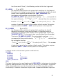


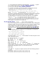


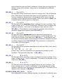


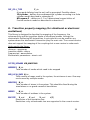


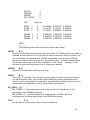

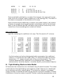
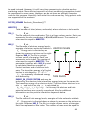

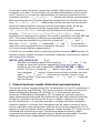


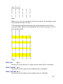


![[ケーススタディ報告書] eDIPS-単層カーボン](http://vs1.manualzilla.com/store/data/006576140_3-f8beca92e422db5ab5db1c5c22753b09-150x150.png)