Download Vimpacct tool v1.0 - University of California, Irvine

User Manual
Vimpacct tool v1.0
Jiwon Hahn, Dexin Li, Qiang Xie
Dept. of Electrical Engineering & Computer Science
University of California
Irvine, CA 92697-2625 USA
{jhahn, dexinl, qxie}@uci.edu
December 15, 2003
Contents
1
Introduction
3
2
An Overview of Vimpacct
6
I
User Manual
7
1
Tool Flow . . . . . . . . . . . . . . . . . . . . . . . . . . . . . . . . . . . . . . . . . . . .
8
2
Input Format . . . . . . . . . . . . . . . . . . . . . . . . . . . . . . . . . . . . . . . . . .
10
2.1
Application Model . . . . . . . . . . . . . . . . . . . . . . . . . . . . . . . . . . .
10
2.2
System Model . . . . . . . . . . . . . . . . . . . . . . . . . . . . . . . . . . . . .
15
3
Control Panel . . . . . . . . . . . . . . . . . . . . . . . . . . . . . . . . . . . . . . . . . .
19
4
Main Window . . . . . . . . . . . . . . . . . . . . . . . . . . . . . . . . . . . . . . . . . .
21
5
Component Editor . . . . . . . . . . . . . . . . . . . . . . . . . . . . . . . . . . . . . . . .
23
5.1
Menu functions . . . . . . . . . . . . . . . . . . . . . . . . . . . . . . . . . . . . .
23
5.2
Editing the Component List . . . . . . . . . . . . . . . . . . . . . . . . . . . . . .
23
5.3
Editing Power Modes . . . . . . . . . . . . . . . . . . . . . . . . . . . . . . . . . .
24
5.4
Editing Mode Transitions . . . . . . . . . . . . . . . . . . . . . . . . . . . . . . . .
24
Policy Generation and Simulation . . . . . . . . . . . . . . . . . . . . . . . . . . . . . . .
26
6.1
Preparing the input files . . . . . . . . . . . . . . . . . . . . . . . . . . . . . . . .
26
6.2
Start Running . . . . . . . . . . . . . . . . . . . . . . . . . . . . . . . . . . . . . .
26
7
Power Command Dispatch . . . . . . . . . . . . . . . . . . . . . . . . . . . . . . . . . . .
27
8
Interactive Simulation Playback . . . . . . . . . . . . . . . . . . . . . . . . . . . . . . . .
28
8.1
Main Window During the Play Back . . . . . . . . . . . . . . . . . . . . . . . . . .
28
8.2
Real-Time Simulation . . . . . . . . . . . . . . . . . . . . . . . . . . . . . . . . .
29
8.3
Step Simulation . . . . . . . . . . . . . . . . . . . . . . . . . . . . . . . . . . . . .
31
8.4
Animation-only Simulation . . . . . . . . . . . . . . . . . . . . . . . . . . . . . .
33
8.5
Zoom I/O . . . . . . . . . . . . . . . . . . . . . . . . . . . . . . . . . . . . . . . .
33
Power Analysis . . . . . . . . . . . . . . . . . . . . . . . . . . . . . . . . . . . . . . . . .
37
9.1
Power profile . . . . . . . . . . . . . . . . . . . . . . . . . . . . . . . . . . . . . .
37
9.2
Pie Chart . . . . . . . . . . . . . . . . . . . . . . . . . . . . . . . . . . . . . . . .
37
Report Generation . . . . . . . . . . . . . . . . . . . . . . . . . . . . . . . . . . . . . . . .
38
10.1
Report Features . . . . . . . . . . . . . . . . . . . . . . . . . . . . . . . . . . . . .
38
10.2
Report Format . . . . . . . . . . . . . . . . . . . . . . . . . . . . . . . . . . . . .
39
6
9
10
1
II Quick User Guide
11
12
40
Getting Started . . . . . . . . . . . . . . . .
Using the tools . . . . . . . . . . . . . . . .
12.1 Simulating Mission . . . . . . . . . .
12.2 Viewing Results . . . . . . . . . . .
12.3 Generating Report . . . . . . . . . .
12.4 Executing Power Commands . . . . .
12.5 Editing Components . . . . . . . . .
12.6 Interactively Playing Back Simulation
12.7 Debugging the Tool at Run-Time . .
2
.
.
.
.
.
.
.
.
.
.
.
.
.
.
.
.
.
.
.
.
.
.
.
.
.
.
.
.
.
.
.
.
.
.
.
.
.
.
.
.
.
.
.
.
.
.
.
.
.
.
.
.
.
.
.
.
.
.
.
.
.
.
.
.
.
.
.
.
.
.
.
.
.
.
.
.
.
.
.
.
.
.
.
.
.
.
.
.
.
.
.
.
.
.
.
.
.
.
.
.
.
.
.
.
.
.
.
.
.
.
.
.
.
.
.
.
.
.
.
.
.
.
.
.
.
.
.
.
.
.
.
.
.
.
.
.
.
.
.
.
.
.
.
.
.
.
.
.
.
.
.
.
.
.
.
.
.
.
.
.
.
.
.
.
.
.
.
.
.
.
.
.
.
.
.
.
.
.
.
.
.
.
.
.
.
.
.
.
.
.
.
.
.
.
.
.
.
.
.
.
.
.
.
.
.
.
.
.
.
.
.
.
.
.
.
.
.
.
.
.
.
.
.
.
.
41
43
43
43
46
46
49
49
51
Chapter 1
Introduction
Welcome to Vimpacct v2.0, a mission-level energy simulator and analyzer. The name Vimpacct stands for
Visual Integrated Management of Power Aware Computing and Communication Technologies. Vimpacct
enables system-level modeling, optimization, and validation of complex power-aware embedded systems by
offering:
• a generic power model for both digital and analog system components, and application models that
capture the environmental knowledge and the application-specific scenarios.
• the capability to exploit mission-awareness in power saving, in addition to the well-known workloaddriven schemes.
• the capability to run in-situ hardware/software co-simulation by sending the generated power commands to the hardware through CORBA interface.
Software Installation
Required Packages
Vimpacct is a cross-platform software written in Python; it runs on Linux/Unix, Mac OS, and Windows
platforms without changing the code. For running the software with full functionality, the following packages
are required:
• Python v2.2 or higher with Tkinter support
• omniORB v4.0 or higher and omniPRBpy v2.0 or higher
• SpecC compiler v1.2 or higher
However, without omniORB and SpecC packages, you can still partially run the tools. omniORB is used
for the execution of power commands through CORBA interface while SpecC is used for re-compiling the
power models for mission simulation. The rest of the user guide assumes the usage of full functionality and
therefore you should have all packages installed.
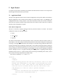
Python is pre-installed on most Unix/Linux and Mac OS platforms. To check whether your python package has Tkinter support, first invoke a Python interpreter by opening the terminal (your system shell) and
type
3
% python
Inside the interpreter, type
% Tkinter
Note that these commands are case sensitive. If no error message appears, then you have the Tkinter module
installed. Similarly, to check whether you have omniORB installed, type
% from omniORB import CORBA
If these packages are not installed, you can download them at
• Python: http://www.python.org
• omniORB: http://omniorb.sourceforge.net/
• SpecC: http://www.ics.uci.edu/∼specc/
How to Install Vimpacct
Here are the quick download links for Vimpacct package:
• http://www.ece.uci.edu/impacct/software/vimpacct-1.0.tar.gz (for Linux/Unix/Mac OS)
• http://www.ece.uci.edu/impacct/software/vimpacct-1.0.zip (for Windows)
To unzip the package, Linux/Unix and Mac OS users can type one of the following commands in the terminal
% gunzip vimpacct-1.0.tar.gz | tar xvf % tar xzvf vimpacct-1.0.tar.gz
Windows users should use Winzip (http://www.winzip.com) or other third party software to unzip the package.
A root directory named jtrs is created on your host. In the rest of this user manual, we will use “$JTRS”
to represent the path to the directory. You do not need to additionally set this path in the shell environment nor build/install the software, since the Python scripts are interpreted rather than pre-compiled. If you
successfully unzipped the package, you are ready to go ahead to the next step.
Setting up the servers
To fully run the tools, you need to have two servers set up. One is the SpecC Simulation Server (SSS), the
other is the CORBA Power Server (CPS).
You can set up each server either on local host, on a remote host. We recommend to set up the servers
on remote hosts (either a Unix/linux machine or an Apple machine with Mac OS X). Let us name your local
host “Host A” and the server host “Host B”. To set up the servers on “Host B”, you need to download and
unzip the same software package on ”Host B” as you did on “Host A”. Run the following command on the
terminal of “Host B” to start the SSS:
% cd $JTRS/daemon
4
% python sc daemon.py 10003
where 10003 is the default port number used by the SSS. The message “Waiting for connection
...” that shows on the terminal confirms that the server is correctly set.
Run the following command on “Host B” to start the CPS:
% $JTRS/corba/mission services server
An IOR (interoperatable object reference) appears in the terminal window and a GUI window of system
diagram pops up. At the moment being, the naming service has not been implemented. You need to manually
pass the IOR to the client side (“Host A”). To do so, on “Host B”, run the following commands to copy the
IOR file securely to “Host A”:
% cd $JTRS/corba
% scp mission service.ior [email protected]:$JTRS/corba/
Each time you restart the CPS, you need to pass the new mission service.ior file to “Host A”. You may
have to explicitly kill the Python processes of the previous server execution, by first finding the PID (process
ID number) of python, by typing on terminal
% ps
then killing the process by typing
% kill -9 PID
How to Use This User Manual
This user manual consists of two parts. Part I provides a comprehensive explanation of Vimpacct tool. It
may be used for thorough understanding of each parts of the tool. Part II is a quick user guide. If the user’s
expectation is the minimal knowledge just enough to be able to use the tool, the user may directly jump to
Part II. The glossary of this manual is provided at the end.
5
Chapter 2
An Overview of Vimpacct
Key Features
Vimpacct provides tools to help you fully optimize and analyze the energy consumption of mission-oriented
embedded systems. The following lists the key features that Vimpacct provides:
• Interpret a high-level mission profile
• Generate a low power schedule
• Simulate schedules via SpecC simulation engine
• Visualize optimal mission power profile
• Interactively play back the power-mode simulation
• Output a comprehensive report that includes power breakdown, component utility, power savings from
the baseline scenario, etc.
• Dispatch power commands to a CORBA power server.
• Let the users edit the power model
These capabilities are supported by the back-end programs including IMPACCT scheduler, SpecC simulator,
and Command dispatcher.
6
Part I
User Manual
7
Application
Model
System
Model
Front-end
VIMPACCT Control Panel
VIMPACCT GUI
Application
Interpreter
Resource
Editor
Power
Analysis
Power
Simulation
Scheduler
Resource
Library
Code
Generator
Simulation
Server
Resource
manager
Corba
Dispatcher
Corba
Server
Report
Generation
Back-end
Policy
Handler
Power
Instrumentation
Figure 1: Block Diagram of Vimpacct Tool Flow
1
Tool Flow
Fig. 1 shows the tool flow of Vimpacct. The top-level partition of the functions is input, front-end, and
back-end. Here, we explain these blocks following the flow of data.
The input to the tool consists of the Application Model and System Model. Application Model captures
the high-level knowledge that is related to mission scenario. System Model captures the architectural information such as the parameters of the hardware resources and dependency among them. Before starting the
tool, these inputs need to be captured in files in the format described in the following section.
Through the control panel of the front-end, the inputs are loaded. Application Interpreter interprets the
XML model into a schedulable format, and the Resource Editor lets the user add/delete/modify parameters
of the System Model.
Then, the back-end of Vimpacct performs scheduling, policy handling and resource management. Scheduler determines the task sequence with exact timestamp; Policy Handler generates mission-aware policies1 ;
Resource Manager determines the power modes of each resource. These three functions generate energyoptimal power command trace.
The finalized resource configuration is stored in Resource Library, and passed to Code Generator, where
the specC simulation code is generated. The generated power command trace from Resource Manager is
dispatched from the CORBA Dispatcher to the CORBA Server. CORBA Server sends the power control
both directly to the Simulation Server and via Power Instrumentation Unit, which is used for hardware cosimulation.
The power command trace passed from Simulation Server is simulated, analyzed, and saved in a report
format. The result is visualized on Vimpacct GUI, which also allows interactive simulation play-back.
The following sections will explain each of the functions in details, in the following order:
1 Policy determines the state of the system. For example, (channel 1 ON, channel 2 OFF) can be a system state. A policy can be
thought of a macro mode of the system, where a macro mode consists of one or more component mode(s); ie., (PA1 ON, Modem1 ON,
GPS ON, PA2 OFF, ...).
8
• 1) input (Section 2),
• 2) front-end (Section 3–4),
• 3) back-end (Section 6–7),
• 4) front-end (Section 8–10)
9
2
Input Format
As Vimpacct uses parameters of both the system and the environment/scenario content, it receives input from
both the application model and the system model.
2.1
Application Model
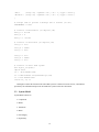
The input of the application model consists of mission configuration, mission profile, and the mission library.
Mission configuration is the an XML file that contains the overall mission scenario. By MAPMgen, this
configuration turns into a message sequence. Since these mission files contain some exclusive information,
both of them are required as Vimpacct input. Mission library also contains exclusive data, those of which not
clarified in either configuration nor profile.
XML Mission Configuration
This part is extracted by mapmgen config.ppt released by Rockwell Collins on 4/14/2003. The mission
configuration contains the following elements:
• mission
• comm manager
• msgprofile
The mission element defines the mission parameters such as start location and time and the sequence of
mission phases. The comm manager element(s) defines parameters that control sending and receiving groups
of messages. The msgprofile element defines what messages are used and message profiles that define sets of
messages and timing values used during a mission phase. Unless otherwise defined all numeric parameters
must be integers. The mapmgen program does not verify the correctness of the configuration before beginning
message simulation. If an error occurs during a waypoint Mapm gen may exit after outputing an incomplete
mission. Examples of errors: a waypoint referencing an undefined profile, a msgtiming element using an
undefined message opcode, or a profile include element referencing an undefined profile. Below, each of
these elements are clearly demonstrated in an XML format.
First, mission is defined by start and phases.
<mission>
<start>
<comment>
Define starting position and time for the mission. Time is in milliseconds. The ticksizemsec is the number of milliseconds the clock
will advance at a time. Each time the clock advances the mission
controller will be notified and will pass the time event to the
comm_manager(s) in order for them to generate messages.
</comment>
<location latitude="42.039" altitude="0" longitude="-91.633" />
<time start="0" ticksizemsec="100" />
</start>
10
<comment>
Define mission phases. The sequence number defines the order in which
the phases are played. This number must start at 0 and increment by 1.
No gaps are allowed in the sequence.
</comment>
+ <phase sequence="0" name="preflight" latitude="42.039" altitude="0"
longitude="-91.633" duration="20000">
+ <phase sequence="1" name="taxi" latitude="42.039" altitude="0"
longitude="-91.625" duration="265000">
+ <phase sequence="2" name="to\_theater" latitude="42.539" altitude=
"5000" longitude="-91.625" duration="571000">
+ <phase sequence="3" name="attack" latitude="42.539" altitude="4000"
longitude="-91.958" duration="313000">
</mission>
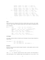
Phases further expand to the following format.
<phase sequence="0" name="preflight" latitude="42.039" altitude="0"
longitude="-91.633" duration="20000">
<comment>
A phase element has attributes defining the destination in
latitude/longitude/altitude measured in degrees and feet and either
a duration in msec or a speed in nautical mph. A phase must have at
least one waypoint. If there are more than one the sequence number
defines their order in the same manner as described in phase. A
waypoint has a duration attribute which defines it’s length in msec.
The last waypoint duration should be 0 and it will last till the end
of the phase. If the duration total for all waypoints exceeds the
phase length the phase will terminate according to the information
in the phase element. If the waypoint total is less and the last
waypoint does not have a duration of 0 the phase will end when that
waypoint is reached. There will be an instantaneous jump in location
to the destination if this occurs.
</comment>
<waypoint sequence="0" duration="0">
<comment>
Waypoints must contain a msgprofile element and one or more
waveform elements. The msgprofile element index attribute
defines the message profile element to use for this segment of
the mission. Within each phase the msgprofiles are accumulative.
At the beginning of a phase the list of messages in use is
cleared. Message timings are then loaded from the profile in the
first waypoint. For each subsequent waypoint the given profile
is added to the message timing list, overwriting settings for
any messages that are currently defined. The waveform attribute
11
indicates which comm_manager will be used for a msgprofile
and thus which waveform will be used to transmit the messages.
</comment>
<msgprofile index=100" waveform=" 0" />
</waypoint>
</phase>
Second, comm manager is defined in the following format.
<comm_manager waveform=0" description="Satcom">
<comment>
Describes parameters needed by a communications manager. waveform is
an integer value that must start with 0 and increment by 1 for each
additional comm_manager. waveform is referenced by a msgprofile element
in a waypoint to indicate which comm_manager is used for the profiles
group of messages. The description attribute is a string without
spaces. The string is output for each message generated by the
comm_manager and describes the waveform used to transmit the message.
request_interval is the time differential between sending groups of
request messages. The round_trip_delay defines how long after a request
group is sent before the associated response is received. Both
parameters are defined in milliseconds. After a request group is sent
the system will not send another until the response is received.
</comment>
<time request_interval="1500" round_trip_delay="1000" />
</comm_manager>
Third, msg profile is defined by messages and profile indices.
<msgprofile>
<comment>
The msgprofile element must include one and only one ’messages’ element
and one or more ’profile’ elements.
</comment>
+ <messages>
+ <profile index="100">
+ <profile index="101">
+ <profile index="200">
+ <profile index="201">
+ <profile index="212">
</msgprofile>
Messages further expand to the following format.
<messages>
<comment>
All messages are described here. Required attributes for a message are
12
opcode, type, size, and family. opcode is a 3 digit hex integer with
leading 0’s. size is a decimal integer. family is a decimal integer
describing what class the message belongs in. type may be one of these
string values: request, response, or broadcast. A broadcast message
is one that the UCAV sends to the ground without being requested. All
other messages must be defined in request/response pairs. request
message must include a ’reply’ attribute that defines the opcode of
the response message. Response messages may include an optional ’gps’
attribute. If this attribute is set to 1 then location coordinates
will be included on the log line whenever the message is sent. The
order which the message elements appear is not important.
</comment>
<message opcode="001" type="request" size="0" reply="801" family="8" />
<message opcode="801" type="response" size="2" family="8" />
<message opcode="003" type="request" size="0" reply="803" family="8" />
<message opcode="803" type="response" size="0" family="8" />
<message opcode="010" type="request" size="0" reply="810" family="2" />
<message opcode="810" type="response" size="16" gps="1" family="2" />
</messages>
Profiles further expand to the following format.
<profile index="100">
<comment>
The profile element contains subelements that define the messages that
are in use during a waypoint leg and the timing parameters used when
sending those messages. Each profile element must include an index
attribute with a unique integer value. This attribute is referenced by
the msgprofile element which is part of a waypoint. The index attribute
must be an integer, but there is no requirement that these numbers be in
order, and the list of profile numbers can contain missing values.
Subelements in a profile can be one of two types: include and msgtiming.
There can be any number of either type of element included. The
msgtiming element defines attributes that control how many of and how
often messages with the given opcode are sent. The interval attribute
defines the time between requests in msec. The repeat attribute is how
many times this message will be sent in a given mission phase. If the
interval is 0 the message will not be sent at all. The include element
must contain two attributes, sequence and index. index references
another profile element. The sequence attribute controls the order in
which the include elements are processed. When a waypoint defines a
profile, that profile element is read in. The system processes the
include elements first and then the msgtiming elements. The result of an
include element being processed is the same as inserting the contents of
the profile it references into the current profile. This include process
13
is recursive, so if the included profile contains include elements, then
those profiles are added as well. Note that there is no checking for
infinite loops, so care must be used when creating an include hierarchy
that has several levels. After the include elements are processed the
system will read the msgtiming elements. The result is that the
msgtiming elements in the current profile will overwrite msgtiming
elements contained in the included profiles. This allows the mission
designer to include a general profile and override particular message
types in this derived profile.
</comment>
<include sequence="0" index="1000" />
<msgtiming opcode="142" interval="1" repeat="1" />
<msgtiming opcode="01f" interval="1" repeat="1" />
</profile>
Mission Profile (.txt)
Mapm gen interprets the XML configuration and generates output in the following format:
timestamp
waveform
opcode
w
x
latitude
longitude
altitude
y
z
The latitude, longitude, and altitude information appears only with a specific opcode, and w, x, y, z are
the parameters not utilized by Vimpacct. The following is an example mission profile.
0.000
0.100
0.100
0.100
0.100
0.100
0.100
Link16
Link16
Link16
Link16
Link16
Link16
Link16
21a
342
346
351
510
3b7
501
2
6
8
4
32
4
6
2
4
2
2
2
1
8
0.305463 -0.338655 0 985097.5683 47.9507
Mission Library (.py)
Mission Library is currently required to be configured manually, although there is a default file for the demo
purpose. It includes:
• Waveform configuration
• Delay for a channel to process a message
• Location of the objects (base station, satellite, and other JTRS objects)
We demonstrate the format in the following sample file.
waveform = {
’Link16’: {’freq’:1000, ’opband’:’hb’, ’ch’: 1, ’type’: ’p2p’},
’Satcom’: {’freq’:225, ’opband’:’lb’, ’ch’: 2, ’type’: ’sat1’},
14
’ATC’:
{’freq’:30, ’opband’:’lb’, ’ch’: 3, ’type’: ’base’},
’MilStar’: {’freq’:30, ’opband’:’lb’, ’ch’: 4, ’type’: ’sat2’}
}
# average time to process a message thru a channel (in sec)
TIMEPERMSG = 0.001
# location of basestation (in degrees, km)
base_la = 42.039
base_al = 0
base_lo = -91.633
# location of satellites (in degrees, km)
sat1_la = 23.0
sat1_al = 35000
sat1_lo = 58.6
sat2_la = 25.5
sat2_al = 38000
sat2_lo = 52.5
# location of other JTRS system
def object_loc(time):
import math
la = 30+0.000001*time
al = 1000+10*math.sin(time*math.pi/720)
lo = 55+0.000001*time
return la, al, lo
Although we assume the location of the other JTRS system as a function over time for now, a mechanism
provided by the communication protocol will enable the system to track the real location.
2.2
System Model
System Model consists of
• Components
• Modes
• Transitions
• Macro
• PowerSupply
• Dependency
15
Components
Components include list of the entire power manageable2 hardware resources in the system and their short
name as shown in following example.
Components= {
’md’: ’Modem’,
’ts’: ’Transciever’,
’pa’: ’Power Amplifier’,...
}
Modes
Modes specify the power mode of each components, each mode having for parameters: metric, tag, power,
para. Metric specifies the application specific information, ie., transmission power of PA for required level
of SNR (Signal-to-Noise Ratio). Tag specifies the active/idle type of mode. Power specifies the actual power
consumption level of the mode considering the efficiency of the real hardware. Para specifies the ideal power
consumption level of the mode. Below shows an example.
Modes= {’md’: {’ON’: {’metric’: ’-’, ’tag’: ’idle’, ’power’: 4.0, ’para’: ’-’},
’OFF’:{’metric’: ’-’, ’tag’: ’idle’, ’power’: 0.01, ’para’: ’-’},
’STB’: {’metric’: ’-’, ’tag’: ’idle’, ’power’: 1.0, ’para’: ’-’}}
’ts’: {’ON’: {’metric’: ’-’, ’tag’: ’idle’, ’power’: 25.0, ’para’: ’-’},
’OFF’:{’metric’: ’-’, ’tag’: ’idle’, ’power’: 0.01, ’para’: ’-’},
’STB’:{’metric’: ’-’, ’tag’: ’idle’, ’power’: 0.1, para’: ’-’}},
’pa’: {’RX’: {’metric’: 6.99, ’tag’: ’idle’, ’power’: 5, ’para’: 5.0 },
’OFF’:{’metric’: -20.0, ’tag’: ’idle’, ’power’: 0.01, ’para’: 0.01},
’STB’: {’metric’: 0.0, ’tag’: ’idle’, ’power’: 1.0, ’para’: 1.0},
’TL1’: {’metric’: 9.4, ’tag’: ’idle’, ’power’: 8.7, ’para’: 1.0},
’TL2’: {’metric’: 16.23, ’tag’: ’idle’, ’power’: 42, ’para’: 10.0},
’TL3’: {’metric’: 25.71, ’tag’: ’idle’, ’power’: 372, ’para’: 100.0},
’TH1’: {’metric’: 9.4, ’tag’: ’idle’, ’power’: 8.7, ’para’: 1.0},
’TH2’: {’metric’: 16.23, ’tag’: ’idle’, ’power’: 42, ’para’: 10.0},
’BYP’: {’metric’: 7.3, ’tag’: ’idle’, ’power’: 5.37, ’para’: 0.1}},
...
}
Transitions
Transitions specify the mode transition overhead. Similar to Modes, power and para is defined, and time
specifies the worst case delay of the transition. Below shows an example. Note that para is an optional field.
Transitions = {
’md’: {’STB_OFF’: {’power’: 1.0, ’para’: ’-’, ’time’: 0},
’ON_STB’: {’power’: 4.0, ’para’: ’-’, ’time’: 100},
2 more
than one power mode
16
’ON_OFF’: {’power’: 4.0, ’para’: ’-’, ’time’: 0},
’STB_ON’: {’power’: 2.5, ’para’: ’-’, ’time’: 0.1},
’OFF_ON’: {’power’: ’4.0’, ’para’: ’-’, ’time’: ’50’},
’OFF_STB’: {’power’: ’4.0’, ’para’: ’-’, ’time’: ’50’}},
’ts’: {’STB_OFF’: {’power’: 0.1, ’para’: ’-’, ’time’: 0},
’ON_STB’: {’power’: 25.0, ’para’: ’-’, ’time’: 100},
’ON_OFF’: {’power’: 25.0, ’para’: ’-’, ’time’: 0},
’STB_ON’: {’power’: 12.5, ’para’: ’-’, ’time’: 0.1},
’OFF_ON’: {’power’: ’25.0’, ’para’: ’-’, ’time’: ’50’},
’OFF_STB’: {’power’: ’25.0’, ’para’: ’-’, ’time’: ’50’}},
...
}
Macro
Macro specifies the power consumption of macro modes. Each macro mode is given a name, such as ‘MAIN’
in the below example, and have the consisting components listed, with the formula for calculating the macro
power consumptions.
Macro = {
’MAIN’
: ([’dc’, ’gu’, ’bi’], ’dc+gu+bi’),
’MAIN/0.85’ : ([’dc’, ’gu’, ’bi’], ’(dc+gu+bi)/0.85’),
’MAIN/0.7’: ([’dc’, ’gu’, ’bi’], ’(dc+gu+bi)/0.7’),
’BLK’ : ([’ts’, ’md’, ’bp’], ’ts+md+bp’),
’BLK/0.9’: ([’ts’, ’md’, ’bp’], ’(ts+md+bp)/0.9’),
’RED’ : ([’ri’, ’rp’, ’eu’], ’ri+rp+eu’),
’RED/0.9’: ([’ri’, ’rp’, ’eu’], ’(ri+rp+eu)/0.9’) }
PowerSupply
PowerSupply specifies the formula to calculate the power consumption of the power supply components, as
shown as below.
PowerSupply = { ’bw’: {’ON’:’BLK/0.9’},
’rw’: {’ON’:’RED/0.9’},
’mw’: {’ON’:’MAIN/0.85’, ’STB’:’MAIN/0.7’}
}
Dependency
Dependency specifies the mode constraints among the components. A mode dependency follows one of the
following two formats:
c0.m0: [c1.m1, ’ ’]
c0.m0: [c1.m1, c2.m2, op]
where ci , mi , i = 0, 1, 2 represents a component and a power mode, respectively. The mode dependency is
used to check whether c0.m0 is a valid mode setting. The first statement says c0 is in m0 only if c1 is in
17
m1. In other words, if c1 is not in m1, c0 cannot be in m0. The second statement says c0 is in m0 only
if c1.m1 op c2.m2 is true. ci .mi is true if the component ci is in the mode mi . op is a logical operator
among AN D, OR, XOR. See the below example. The first constraint says “The PA is on only if the domain
controller is on and main power is on”. The last constraint says “The domain controller is on only if the main
power is on”.
Dependency = {
’pa.ON’:
’ts.ON’:
’bp.ON’:
’dc.ON’:
[’dc.ON’,’mw.ON’,’&’],
[’dc.ON’,’bw.ON’,’&’],
[’dc.ON’,’bw.ON’,’&’],
[’mw.ON’,’ ’] }
18
Mission Load
Policy Generation
Profile Load
Power Profile View
System Power View
Report Generation
Component Edit
Program Exit
Component Load
Profile Simulation
Energy Breakdown
Command Dispatch
Simulating Wheel
Speed Scaling Bar
Figure 2: Conrol Panel
3
Control Panel
Control Panel shown in Fig. 2 is used for running each function of Vimpacct. Table 1 shows the mapping of
icon to menu, and their brief description. The rows are presented in the order of the usage (tool flow).
In the users point of view, C1–C3 are used for loading the inputs, C4,C5,C10,C11 are used for running
the tools, and C6–C9 are used for viewing the results. The simulating wheel and the scaling bar are used
in controlling the user-interactive simulation play back, which will be explained in Section 8. Complete
explanation for each control functions will be presented in Section 5–10.
19
Icon
File Menu
Descryption
C1
File→Load Library
Load the component library, ie., mycomplib.py
C2
File→Load Mission
Load the component library, ie., mission7.txt
C3
File→Load Profile
Load a pre-simulated mission (optional)
C4
Tools→Policy Generation
Generate power control commands.
C5
Tools→Profile Simulation
Run the simulation
C6
Tools→Display Component Power
View the channel/component power profile
C7
Tools→Display Energy Profile
View the energy breakdown
C8
Tools→Display System Power
View the system power profile
C9
Tools→Generate Report
Generate the summary report
C10
Tools→Run Dispatcher
Run the CORBA client dispatcher
C11
Tools→Edit
Open the component editor
C12
File→Exit
Exit the Program
Table 1: Control Panel Functions
20
Simulation Toolbar
Control
Panel
Mode Simulation
Mission Animation
PA and Mission Status
System Power Profile
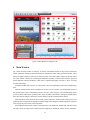
Figure 3: Main Window of Vimpacct Tool
4
Main Window
Fig. 3 shows the main window of Vimpacct. It consists of Simulation Toolbar on top, and four frames that
consist of Mission Animation, Mode Simulation, PA and Mission Status, and System Power Profile. These
frames are tightly coupled. In other words, change of status in one frame applies changes in all other frames
also. This window is utilized for visualizing the simulation, and thus, is related to the interactive play back
(rather than back-end auto-simulation), which will be explained thoroughly in Section 8. Here, we briefly
introduce their usages.
Simulation Toolbar that consist of 11 control icons is used for controlling the interactive simulation play
back.
Mission Animation frame shows the high-level scenario view of a mission. The background consists of
four possible places of the communicating objects: land, sky, water, and space. The communicating objects
are base stations, JTRS objects (possibly UAVs, ships, and tanks), and satellites. During the simulation play
back, these objects animate to show their location, distance, and the communication activities.
Mode Simulation frame shows the layout of the system architecture. In this window, all the power manageable hardware components are displayed, and they change color during the simulation play back. Different
colors specify the power mode of the components.
PA and Mission Status frame consists of four sub-frames: top, middle-left, middle-right, and bottom. The
top frame shows the elapsed time counted from the beginning of simulation, and the current communica21
tion distance. The middle-left frame shows the status of each PAs among TX/RX/IDLE. The middle-right
frame shows the current location of the main JTRS object (our system). The bottom frame shows the power
consumption level of PA in terms of dBW.
System Power Profile displays the entire simulation profile, with Y-axis as system power (Watt) and Xaxis as time (sec). It lets the user analyze the system status at the peak power usages.
22
5
Component Editor
The Component Editor is a user front-end for the component library. The User can use the Component
Editor to create/edit component models which are then compiled into simulatable SpecC models for power
simulation.
The Component Editor allows the user to
• Create a component library
• Add/remove components to a component library
• Change the component ID and the component description of a component
• Add/remove power modes of a component
• Change the name and attributes of a power mode
• Add/remove mode transitions of a component
• Change the name and attributes of a mode transition
• Generate the SpecC model of a component library3
The main window of the Component Editor has three columns. The left column allows the user to edit
the component list of a library. The middle column allows the user to edit the power modes of a component.
The right column allows the user to edit the mode transitions of a component. We will first briefly introduce
the menu functions, followed by the descriptions of the functions in each column.
5.1
5.2
Menu functions
File→New Library...
Create a new library.
Save the currently opened library if it is modified.
File→Open a Library...
Open an existing library.
Save the currently opened library if it is modified.
File→Save
Save the current library.
File→Save As...
Save the current library with a specified name.
File→Close
Close the current library. Save it if modified.
File→Exit
Exit the window.
Tool→SpecC Code Gen...
Code generation of the SpecC power model.
About→Help
Empty stub.
Editing the Component List
The left column of the main window has a list window to show the component list. Once a library is loaded,
the component ID’s and names are listed. The component ID is a short name of a component without a space.
The component name is an elaborated name the user defined for the component.
3A
SpecC compiler v1.2 or higher is required; a GCC compiler v2.9x is required.
23
5.3
Add a component4
Type in the component ID in the short empty field.
Type in the component name in the long empty field.
Click the Add button below the short empty field.
Edit a component
Click a component name.
Type in the updated information.
Click the Edit button below the long empty field.
Remove a component
Click a component name.
Click the Remove button below the long empty field.
Editing Power Modes
Double-click a component name in the left column brings up the available power modes and mode transitions
of the component in the middle and right columns, respectively. The middle column allows the user to edit
the power modes of a component. There are four attributes of a power mode:
• Mode name
• Power Consumption
• Parameter
• Metric
The Power Name must be in capital letters without spaces. The Power Consumption can be either a number
(integer or floating-point), or a formula. The Parameter is used as a variable when the Power Consumption
is represented as a formula. The Metric is application-specific, representing an application-level requirement
or constraint,e.g., quality of service, signal to noise ratio, etc..
5.4
Add a mode
Type in ALL the four attributes in the corresponding fields
(use hyphen if it is empty).
Click the Add button at the bottom of the column.
Edit a mode
Check a mode name.
Type in the updated information.
Click the Edit button at the bottom of the column.
Remove a mode
Click a mode name.
Click the Remove button at the bottom of the column.
Editing Mode Transitions
Double-click a component name in the left column brings up the available power modes and mode transitions
of the component in the middle and right columns, respectively. The right column allows the user to edit the
mode transitions of a component. There are five attributes of a mode transition:
• From mode
• To mode
• Time
• Power
24
• Parameter
The From mode and To mode are two power modes of a mode transition, as the name suggested. The Time
and Power are the time delay and the power consumption of the mode transition, respectively. The Parameter
is used as a variable when either or both of the Time and Power attributes are represented as a formula.
Add a mode transition
Type in ALL the five attributes in the corresponding fields
(use hyphen if it is empty).
Click the Add button at the bottom of the column.
Edit a mode transition
Check a From mode name.
Type in the updated information.
Click the Edit button at the bottom of the column.
Remove a mode transition
Click a From mode name.
Click the Remove button at the bottom of the column.
25
6
Policy Generation and Simulation
Vimpacct policy generation is based on Decoupled Power Management Architecture(DOMA). The main idea
is to decouple system-level policy making from the architectural level device control. For more information
on the DPMA, please refer to [?].
Vimpacct mission simulation is performed using SpecC power models. The advantage of using SpecC
power models is the powerful support for concurrent simulation and sychronized communication between
software modules.
6.1
Preparing the input files
To run the poligy generation, the user need to prepare the mission profile files and the component library file.
Put the mission profiles both in the XML format and in the text format (generated by MAPMgen.exe) in
$JTRS/missionlib/. Some sample files are already in there. Refer to the sample files for the file format.
Put the component library in $JTRS/complib/. The component library is a Python script. Users familiar
with Python language can manually edit the library file, Refer to $JTRS/complib/mycomplib.py as an example. General users can use the GUI (Component Editor) to create/edit a component library without knowing
Python.
6.2
Start Running
When the user starts the policy generation, some text messages are printing on the terminal window showing
the progress of the policy generation. Depending on the size of the mission, the policy generation may take a
while. When it shows “Mode transitions generated by DPMA”, the process is completed.
Once the policy generation is completed, the mission simulation can be started. The power commands
are sent to the SpecC simulation Server for power simulation. Some text messages are printed out on both
the client side and the server side. Once the mission simulation is done, the system power profile appears on
the Main Display Window.
26
7
Power Command Dispatch
We can send the generated power commands to a virtual platform for execution. The CORBA is used as the
common interface between the power manager and the virtual platform.
The CORBA server is written in C++, with a Python wrapper that interacts with a graphic user interface
as the virtual platform. The server receives the power commands of individual components from the client,
execute the commands on the server and displays the power mode changes on the graphic user interface.
The CORBA client is written in Python. It reads a static power schedule from a file in which each power
command is associated with a time stamp. The commands are dispatched at the real time through the CORBA
interface to the server.
The CORBA client identifies the server by the means of the Interoperatable Object Reference (IOR)
which is produced on the server side once the server is started. Therefore the IOR should be sent to the client
prior to its dispatch of power commands.
To start the CORBA server, type the following commands in a terminal on the server host:
%cd $JTRS/corba
% python py mission server.py
To send the IOR to the client side, run the following commands in a separate terminal on the server host:
% cd $JTRS/corba
% scp mission service.ior [email protected]:$JTRS/corba/
where client.host.name is the host name on the client side and username is the user account name
on the client side. Jiwon: is this correct? (’name’ in the address?)
To start the command dispatch on the client side, choose Tools→Run Dispatcher or click
on the
Control Panel. You will see text messages printing to the shell windows on both server side and client side.
At the same time, the commands are executed on the virtual platform on the server side and power modes
transitions are shown in the graphic window on the server side.
The command dispatch is completed when it reaches the end of the power schedule.
To shut down the CORBA server, the user need to explicitly identify and kill the server process.
% ps -ef | grep python
% kill -9 serverProcessNumber
where serverProcessNumber is the process number of the server process.
27
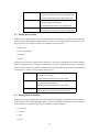
Figure 4: The Main Window Display during Playback
8
Interactive Simulation Playback
Interactive Simulation Playback allows the user to observe the simulation in controlled granularity. The play
back is controlled by the toolbar on top of the main window as shown below, and the simulating wheel on the
control panel (Fig. 1).
Real-Time
Simulation
Step
Simulation
Profile Zoom
Animation-only
Simulation
Exit
We will first explain how to interpret the main window display during the play back, then explain the
usage of each group of controls.
8.1
Main Window During the Play Back
Fig. 4 shows the main display window during the simulation playback. As introduced in Section 4, it shows
the mission animation, mode simulation, PA and mission status, and system power profile frame inside the
quadrant.
In the Mission Animation frame, shown in Fig. 5, the JTRS object moves during the mission, and the
28
Figure 5: Mission Animation during Playback
communication links appears in colored lines. Each color (dark red, red, orange, and yellow) indicates one
channel among four. When the link is accomplished, the communicating objects turns into red.
The Mode Simulation frame, shown in Fig. 6 shows the system architecture. When the simulation is
initialized, each components show their original colors. During the simulation, they switch colors showing
their mode status. Gray indicates OFF mode, blue indicates IDLE mode, light pink indicates RX mode (in
PA only), and red indicates FULL ON mode.
The PA and Mission Status during Playback frame shown in Fig. 7 shows the time, communicating
distance, PA status, location, and the power consumption level of PA. On this example, the elapsed time is
43.2 sec, the distance between active link (where the PA is transmitting message) is 37637 km. PA15 and PA3
are in IDLE6 mode, PA2 is in TX mode, and PA4 is in RX mode. The current location of our JTRS system
is displayed in latitude, longitude (in degrees), and altitude (in km). We can see that PA2 power level bar has
reached the maximum amount, since it is transmitting to a far distance.
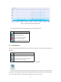
The System Power Profile frame shows the profile of the system through the entire mission as shown in
Fig. 8. This particular mission has the interval of approximately 80 sec. The red anchor line proceeds to the
right while the simulation plays.
8.2
Real-Time Simulation
Real-time simulation lets the user play back a mission at the speed of real time. The user can start, fast
forward, pause, stop, and reset the mission. At any time, the user may either jump forward or backward onto
any timestamp of a mission by clicking on a desired point on the power profile window. For example, if the
user clicks on a point around 40.0 sec as shown on the top of Fig. 9, the anchor (red line) will move to that
point, and all four frames will display the mission status at 40.0 sec.
5 PA
for channel 1
for the PA is determined by whether message is going through the PA or not. ACTIVE includes RX (receiving) or
TX (transmitting) mode.
6 IDLE/ACTIVE
29
Figure 6: Mode Simulation during Playback
Figure 7: PA and Mission Status during Playback
30
Figure 8: System Power Profile during Playback
The following table shows the description of the real-time simulation control.
Icon
Description
Play-back the mission on real-time
Fast-forward the mission
Pause the real-time play-back
Stop a real-time play-back
Return to initial state of the mission
8.3
Step Simulation
The user can also play step simulation to observe the states in finer grain. The below controls support step
simulation.
Icon
Description
Go to the beginning state of a mission
Step backward to the previous state of a mission
Step forward to the next state of a mission
Go to the final state of a mission
Alternatively, the user may use the Simulation Wheel, on the control panel:
The user can first set the speed of the wheel, by controlling the scale bar, where 1 represents the fastest
speed and 20, the slowest speed. Then, the user manually rolls the wheel either clockwise or counter clockwise to proceed the simulation or roll-back the simulation, respectively (see Fig. 10).
31
Click to set anchor
Figure 9: Setting the Anchor Point
32
Roll to manully simulate
Figure 10: Manual Simulation by Rolling the Simulating Wheel
8.4
Animation-only Simulation
Animation-only simulation lets you observe the mission scenario at a glance. Independent of system power
mode, it proceeds the simulation in a rapid speed – faster than fast forward function of real-time simulation.
This functionality is controlled by the following two icons.
Icon
Description
Run the animation of a mission only (fast)
Stop the animation of a mission only
8.5
Zoom I/O
Zoom functions let the user observe the system mode in multi-granular way. Since the time granularity of the
mode transitions is in milliseconds, and the mission length can reach longer than 10 hours, the zoom in/out
is an important functionality. It is controlled either by clicking the below icons, or directly selecting an area
by mouse on the power profile frame.
Icon
Description
Zoom in one step of the system power profile
Zoom out one step of the system power profile
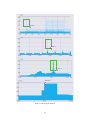
Here, we show the usage of these functions by an example. Fig. 11 is an initial state after a mission load.
On the power profile, it is observed that there is a power glitch around timestamp of 10 sec. To discover the
exact system state that is causing the glitch, the user may click and drag the mouse to select the area to zoom
in (see Fig. 12). The user can repeat zooming in until the desired view is reached. In Fig. 12, the original
33
Figure 11: Initial State after Loading the Mission
profile is zoomed in three times. Then, the user can click on a point (10.101 sec) to exactly set the anchor.
Fig. 13 shows the global view of the main window. Now, the user can see the reason why there seemed
to be a power glitch; 1) there are many communication activities going on at the moment with three PAs on
active power states, 2) more than half of the system is fully ON. Without zooming in, it is hard for the user to
set the anchor to the exact point where this state occurs.
34
zoom 1
zoom 2
zoom 3
set anchor
Figure 12: The Usage of Zoom In
35
Figure 13: The Result of Fig. 12
36
9
Power Analysis
Once the mission simulation is completed, the information about power break-down of channels as well as
that of components are available for analysis.
9.1
Power profile
on the Control Panel.
To obtain the power profiles, choose Tools→Select Component Power or click
A new window of channel-level power profiles shows up, each track representing the power profile of a
channel. The user can zoom in or zoom out the power profile by clicking the corresponding buttons at the top
of the window. The user can double-click a track to view a lower level (component-level) of power profiles.
View more details of the profiles
View less details of the profiles
Generate an EPS file of the window
Exit the window
9.2
Pie Chart
To obtain the pie charts, choose Tools→Display Profile menu item or click
on the Control Panel.
The pie chart shows the power break-down of the system by channels. Double-click each portion in the
energy pie chart to view each channel’s energy break-down by components.
The user can choose to export the power profiles or pie charts to EPS files by clicking
37
.
10
Report Generation
The user can use the report generation tool to generate customized text reports and figures.
10.1
Report Features
Start the report generation tool by choosing Tools→Generate Report or click
3, row 3).
on the Control Panel (col
The user can generate the following items in the text report:
• General mission information
• Channel-level energy information
• Component-level energy information
• Channel-level command information
• Component-level command information
The user can set the sorting criteria for the energy information:
• by channel
• by component name
• by energy usage
• by time usage
The user can set the sorting criteria for the command information:
• by channel
• by component name
• by command count
The user can generate the following figures in the encapsulate postscript EPS format:
• System power profile
• Channel-level power profile
• Component-level power profile
• System-level pie chart
• Channel-level pie chart
The user can save the text report by clicking the Save button. To load a previously stored text report, click
Load button. The EPS figures are stored at $JTRS/report/eps directory.
38
10.2
Report Format
Here is the description of the fields in the report.
General
Mission Name
Mission Length
Total No. of messages
Total No. of commands
Total waveforms
Total channels
Total components
System peak power
Total energy
Baseline Energy
Energy savings
The name of the mission
The length of the mission in seconds
Number of messages in the input mission profile
Number of power commands generated by the tool
total number of waveforms
total number of channels
total number of power-manageable components
Peak power consumption over the mission, in Watt
Total energy after power management, in Joule
Energy consumption without power management, in Joule
Energy savings in percentage
Channel-level energy statistics
Channel
Energy
Percentage
Channel number (0 is shared resources)
Energy consumption of the channle, in Joule
Energy percentage of the channel
Component-level energy statistics
Component Name
Energy(J)
Energy(%)
Ontime(s)
Ontime(%)
Component description
Energy consumption of the component, in Joule
Energy percentage of the component, in percentage
Time in which component has non-zero workload, in second
Time percentage of Ontime, in percentage
Channel-level command statistics
Channel
Command(#)
Command(%)
Channel number (0 is shared resources)
Number of commands for that channel
Percentage of the number of commands
Component-level command statistics
Component Name
Command(#)
Command(%)
Component description
Number of commands for that component
Percentage of the number of commands
39
Part II
Quick User Guide
40
This quick user guide contains the following subsections:
• Getting started
• Using the tools
• Viewing the results
• Generating reports
• Executing power commands
• Editing components
• Interactively playing back the simulation
• Debugging the tool at run-time
11
Getting Started
To get started, you first need to prepare the input files: mission files (mission configuration and mission
profile), and component library. Mission profile is pre-generated by passing mission configuration through
MAPMgen. Put the mission filesin $JTRS/missionlib/. For the demo purpose, some sample files already exists. Refer to the sample files to get the file format. Let us assume the mission to be executed is “mission7”, so
we place mission7.xml and mission7.txt in $JTRS/missionlib/ directory. Put the component library
in $JTRS/complib/. The component library is a Python script. Users familiar with Python can manually edit
a library file. Users may use the GUI (Component Editor) to create/edit a component library without knowing
Python. For the demo purpose, the component library mycomplib.py is already in there.
Now we can run Vimpacct by entering the directory and run the main script as following.
% cd $JTRS/jtrsgui/code/
% python jtrsgui.py
As a quick Vimpacct splash disappears, the Control Panel (the small window on the left) and the Main
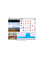
Display Window (the large window on the right) show up (see Fig. 14). Main Display Window consists of a
simulation toolbar on the top, and four frames underneath that display:
• Mission Animation
• Mode Simulation
• PA and Mission Status
• System Power Profile
Fig. 15 shows the icons of the control panel that are used to speed up access to the tools. The following
subsections will reveal the functionalities of the corresponding tools.
41
Simulation Toolbar
Control
Panel
Mode Simulation
Mission Animation
PA and Mission Status
System Power Profile
Figure 14: GUI: the Control Panel and the Main Display Window.
Mission Load
Policy Generation
Profile Load
Power Profile View
System Power View
Report Generation
Component Edit
Program Exit
Component Load
Profile Simulation
Energy Breakdown
Command Dispatch
Simulating Wheel
Speed Scaling Bar
Figure 15: Control Panel
42
12
Using the tools
Vimpacct offers various tools for optimizing, simulating, and analyzing energy consumption of a mission.
We will explain these tools in the sequential order, which let you explore full functionality of Vimpacct.
12.1
Simulating Mission
This subsection shows the sequence of using the tools related to the auto-simulation of a mission. By followStep
File Menu
Explanation
1
File→Load Library
Load the component library, ie., mycomplib.py
2
File→Load Mission
Load the component library, ie., mission7.txt To find the
library, you should navigate to $JTRS/missionlib
3
Tools→Policy Generation
Generate power control commands. Depending on the size of
the mission, this may take a while.
4
Tools→Profile Simulation
File→Save Profile
Run the simulation; on completion, the system components
and the system power profile will appear on the Main Window
(Fig. 16)
Save the simulation result as a user-defined name for later use
File→Load Profile
Load a pre-simulated mission
5
Icon
–
6
Table 2: Steps for Mission Simulation.
ing the steps shown in Table 2, you can simulate/load/save a mission.
In the meanwhile, you can check the progress in the terminal window in which you started the GUI.
For example, when the process of Step 3 is completed, you will see a terminal message, “Mode transitions
generated by DPMA”. Please make sure the previous process is finished, before executing the next step. The
simulated power profile is generated after Step 4, and saved as “result.txt” as default, in $JTRS/.temp.
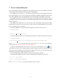
12.2
Viewing Results
The result of simulation is energy analysis of the optimized system for the mission. It could be observed in
two different ways: system power profile in 2D energy/time graph and energy breakdown in pie charts. Both
ways offer multi-level analysis, by letting users choose to zoom into channel-level view, and zoom out to
system-level view.
The below table shows how to view the results.
Icon
File Menu
Description
Tools→Display System Power
View the system power profile
Tools→Display Component Power
View the channel/component power profile
Tools→Display Energy Profile
View the energy breakdown
Table 3: Two Ways to Observe the Optimized Energy
43
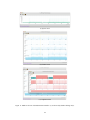
Figure 16: Main Window with System Components and Power Profile Loaded
System Power Profile View
By selecting the first icon/menu in Table 3, a system view of power profile pops up as shown in Fig. 17 (a).
Channel/Component Power Profile View
The second icon/menu in Table 3 will instantiate a new window entitled “JTRS Power Profile Simulator” as
shown in Fig. 17 (b). This is the profile view of the channels. By double clicking a blue area of a channel,
another window will pop up, showing the detail component power of the channel as shown in Fig. 17 (c). In
these window, there are four icons on the top. The following table shows the usage of each.
Icon
Description
Zoom in the power profile within the same system/component level
Zoom out the power profile within the same system/component level
Export the displayed power profiles to an EPS file
Close the window
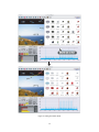
Energy Breakdown View
By clicking the third icon/menu of Table 3, a window showing a pie chart of system power breakdown will
pop up. Double-click each portion in the energy pie chart to view the energy breakdown of a lower level, as
shown in Fig. 18.
44
(a) System View
(b) Channel View
(c) Component View
Figure 17: Multi-Level View of Simulated Power Profiles. (c) is observed by double-clicking on (b).
45
double
click
Figure 18: Pie charts: Energy breakdown. Double-click a slice to navigate a level down.
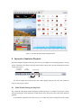
12.3
Generating Report
Icon
File Menu
Tools→Generate Report
Comment: dexin, I don’t see ”Tools→Generate Report” on the Tools menu right now. is it included in
the latest version?
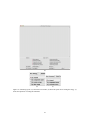
By the above icon or menu, you can generate a report of the simulation profile A new window will pop up
and you can specify the items you want to generate in the report by selecting or deselecting the checkboxes
(see Fig. 19 (a)). You can specify the sorting criteria by selecting the pull-down menu at the bottom of the
window (Fig. 19 (b), (c)). The default is set to sort by channel. When the selection is done, click “Generate
Report” button to generate the report in the main text window. The generated report will look like Fig. 20.
You can save the report by clicking the “Save Report” button. You can load a previously stored report by
clicking Load button. After done, close the window.
12.4
Executing Power Commands
Now you can run the Command Dispatcher to send the power commands to the CORBA Power Server
through a CORBA interface. Click on the below icon or menu to run the CORBA client.
Icon
File Menu
Tools→Run Dispatcher
You will see text messages printing to the shell windows on both server side and client slide hosts as
shown in Fig. 21. At the same time, the commands are executed on the virtual platform on “Host B” and
power modes transitions are shown in the server-side GUI.
46
(a)
(b)
(c)
Figure 19: Generating report. (a) is the main text window. (b) shows the option list of sorting the energy. (c)
shows the option list of sorting the command.
47
Figure 20: The Generated Report
48
Figure 21: Executing power commands through a CORBA client.
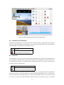
12.5
Editing Components
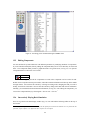
You can simulate the system architecture with different parameters by modifying attributes of components.
If you are familiar with Python, directly editing the component library file in a text editor may be easier and
faster. The Component Editor provides a graphical interface for general users (see Fig. 22). To open the
Component Editor use the below icon or menu.
Icon
File Menu
Tools→Edit
A new window pops up and all the components are listed in the Component List box on the left side.
Double-click a component and its power modes, and mode transition information will show up in the middle
and right frames. You can then edit a mode by selecting an existing mode, changing the field you want to
modify, and click the edit button. You can also add a mode by filling in the fields and click the add button.
Similarly, you can add and edit mode transition information (see Fig. 22). After editing the components, you
can save the component library by choosing File→Save or File→ Save As. 7
12.6
Interactively Playing Back Simulation
Now, let us go back to the main display window (Fig. 14). You will find the following toolbar on the top of
the window.
7 A code generation process needs to be executed to provide the updated power model for the simulation server. To perform the code
generation, a SpecC compiler v1.2 or higher and a GCC compiler v2.9x are required.
49
Figure 22: Component Editor.
Real-Time
Simulation
Step
Simulation
Run-Time
Debugging Tool
Profile Zoom
Animation-only
Simulation
About..
Exit Window
These tools are used for interactive play-back of a simulation. They are separated in groups that have
different functionalities.
Real-Time Simulation
Real-Time Simulation provides a way to simulate the play-back at the speed of the real time. Although it
proceeds automatically once simulation is initiated, you have the control to pause/stop and restart the simulation. You may also speed up by the usage of fast forward. You can also reset the simulation. The following
table summarizes the functions.
Icon
Description
Play-back the mission on real-time
Fast-forward the mission
Pause the real-time play-back
Stop a real-time play-back
Return to initial state of the mission
50
Step Simulation
The step simulation allows you to observe the detailed mode transition of each component with respect to
time. It also provides the high-level view of a mission by the time-accurate animation of communicating
objects and the status of time, location, distance, and a mission-aware component (PA). Step simulation is
controlled by the following icons.
Icon
Description
Go to the beginning state of a mission
Step backward to the previous state of a mission
Step forward to the next state of a mission
Go to the final state of a mission
Alternative to these controls, you can also use the simulating wheel on the Control Panel (Fig. 15) to
manually playback the mission scenario. You can tune the slowdown factor by setting the scale bar underneath
where 1 represents the fastest speed and 20 the slowest speed.
During the simulation, you can set a starting anchor anywhere inside the system power profile frame by
clicking at the position you want to start the playback.
Animation-only Simulation
Animation-only simulation lets you observe the mission scenario at a glance. Independent of system power
mode, it proceeds the simulation in a rapid speed – faster than fast forward function of real-time simulation.
This functionality is controlled by the following two icons.
Icon
Description
Run the animation of a mission only (fast)
Stop the animation of a mission only
Etc.
Zoom functions on the main window let you observe into more depth. They work in the bottom right window
that shows system power profile.
Icon
Description
Zoom in one step of the system power profile
Zoom out one step of the system power profile
Exit the main display window
12.7 Debugging the Tool at Run-Time
The text entry box in the toolbar of the main window lets the user dynamically modify the program. This
box is used by the authors for the debugging purpose. However, if the user is familiar with Python and the
Vimpacct code, he/she can also use it to modify the internal variables as well as the GUI itself.
51
Glossary
CPS
dBW
IOR
IMPACCT scheduler
MAPMgen
Mission Configuration
Mission Profile
Power Model
SSS
Terminal
UCAV
CORBA Power Server
decibel referenced to one watt
Interoperatable Object Reference
??
Mission profile generator developed by Rockwell Collins
A mission scenario specified by start time, phases, waveforms, message indices, etc, captured in a pre-defined XML format
A trace of messages ordered by timestamp, which specifies the released time of a message.
??
SpecC Simulation Server
The system shell
Unmanned Combat Airborne Vehicle
52
Bibliography
53