Download NetLogo Tutorial Notes - Operations, Information and Decisions

NetLogo Tutorial Notes
Steven O. Kimbrough
April 11, 2014
Steven O. Kimbrough, kimbrough[at]wharton.upenn.edu
$Id: NetLogo-tutorial-notes.tex 3684 2013-09-09 20:37:28Z sok $
i
ii
Contents
Preface
ix
1 Starters
1.1 Starters . . . . . . . . . . . . . . . . . . . . . . . . . . . . . .
1.1.1 NetLogo world view (main metaphors) . . . . . . . . .
1.2 The Interface Tab . . . . . . . . . . . . . . . . . . . . . . . .
1.2.1 The Observer . . . . . . . . . . . . . . . . . . . . . . .
1.2.2 Inspecting . . . . . . . . . . . . . . . . . . . . . . . . .
1.2.3 Editing the View (and the World) . . . . . . . . . . .
1.2.4 More on Editing the World . . . . . . . . . . . . . . .
1.2.5 Interface Widgets (on the Toolbar) . . . . . . . . . . .
1.2.5.1 NetLogo Interface Tab: The Interface Toolbar: Buttons . . . . . . . . . . . . . . . . . .
1.2.5.2 NetLogo Interface Tab: The Interface Toolbar: Sliders . . . . . . . . . . . . . . . . . . .
1.2.5.3 NetLogo Interface Tab: The Interface Toolbar: Switches . . . . . . . . . . . . . . . . . .
1.2.5.4 The Interface Toolbar: Choosers . . . . . . .
1.2.5.5 The Interface Toolbar: Input boxes . . . . .
1.2.5.6 The Interface Toolbar: Monitor . . . . . . .
1.2.5.7 The Interface Toolbar: Plot . . . . . . . . . .
1.2.5.8 The Interface Toolbar: Output . . . . . . . .
1.2.5.9 The Interface Toolbar: Note . . . . . . . . .
1.2.6 The Interface Toolbar: Plot . . . . . . . . . . . . . . .
1.2.7 Introduce a Bug . . . . . . . . . . . . . . . . . . . . .
1.3 The Info Tab . . . . . . . . . . . . . . . . . . . . . . . . . . .
1.4 The Code Tab . . . . . . . . . . . . . . . . . . . . . . . . . .
1.4.1 Commands and reporters . . . . . . . . . . . . . . . .
1.4.2 Global and local variables . . . . . . . . . . . . . . . .
iii
1
1
1
2
2
2
3
5
5
5
6
6
7
7
7
8
8
8
8
13
14
15
17
17
1.4.3
1.4.4
1.4.5
1.4.6
1.4.7
1.4.8
1.4.9
1.4.10
1.4.11
1.4.12
Comments and line breaks . . . . . . . . . . . . . .
Assignment: Set . . . . . . . . . . . . . . . . . . .
Agent properties, turtles-own, and patches-own
Agentsets . . . . . . . . . . . . . . . . . . . . . . .
Breeds of turtles . . . . . . . . . . . . . . . . . . .
Lists . . . . . . . . . . . . . . . . . . . . . . . . . .
Character strings . . . . . . . . . . . . . . . . . . .
I/O . . . . . . . . . . . . . . . . . . . . . . . . . .
Control flow and logic . . . . . . . . . . . . . . . .
Typical program structure . . . . . . . . . . . . . .
2 Exercise: Testing Strategies in 2×2
2.1 Needed Programming Elements . .
2.1.1 Local and Global Variables
2.1.2 Reporters . . . . . . . . . .
2.1.3 Lists . . . . . . . . . . . . .
2.1.4 Random Numbers . . . . .
2.1.5 Turtles . . . . . . . . . . . .
2.2 Understanding Simple2x2.nlogo . .
2.3 Exercises . . . . . . . . . . . . . .
Games
. . . . .
. . . . .
. . . . .
. . . . .
. . . . .
. . . . .
. . . . .
. . . . .
3 Exercise: Simple animation with turtles
3.0.1 Exercise 1 . . . . . . . . . . . . .
3.0.2 Exercise 2 . . . . . . . . . . . . .
3.0.3 Exercise 3 . . . . . . . . . . . . .
3.0.4 Solutions . . . . . . . . . . . . .
3.0.4.1 Exercise 1 . . . . . . . .
3.0.4.2 Exercise 2 . . . . . . . .
3.0.4.3 Exercise 3 . . . . . . . .
4 Working with Lists
4.1 Basics . . . . . . . . . . . . . . . . .
4.2 Exercise: map and data manipulation
4.2.1 Exercise 1 . . . . . . . . . . .
4.2.2 Exercise 2 . . . . . . . . . . .
4.2.3 Solutions . . . . . . . . . . .
4.2.3.1 Exercise 1 . . . . . .
4.2.3.2 Exercise 2 . . . . . .
4.3 Exercise 3: Probe and Adjust . .
4.4 Exercise 4: Genetic Operators . . . .
iv
.
.
.
.
.
.
.
.
.
.
.
.
.
.
.
.
.
.
.
.
.
.
.
.
.
.
.
.
.
.
.
.
.
.
.
.
.
.
.
.
.
.
.
.
.
.
.
.
.
.
.
.
.
.
.
.
.
.
.
.
.
.
.
.
.
.
.
.
.
.
18
18
19
20
21
22
23
23
24
25
.
.
.
.
.
.
.
.
.
.
.
.
.
.
.
.
.
.
.
.
.
.
.
.
.
.
.
.
.
.
.
.
.
.
.
.
.
.
.
.
.
.
.
.
.
.
.
.
.
.
.
.
.
.
.
.
.
.
.
.
.
.
.
.
.
.
.
.
.
.
.
.
.
.
.
.
.
.
.
.
27
28
28
29
29
29
29
30
30
.
.
.
.
.
.
.
.
.
.
.
.
.
.
.
.
.
.
.
.
.
.
.
.
.
.
.
.
.
.
.
.
.
.
.
.
.
.
.
.
.
.
.
.
.
.
.
.
.
.
.
.
.
.
.
.
.
.
.
.
.
.
.
.
.
.
.
.
.
.
33
34
34
35
36
36
37
39
.
.
.
.
.
.
.
.
.
43
43
44
44
45
45
45
45
46
48
.
.
.
.
.
.
.
.
.
.
.
.
.
.
.
.
.
.
.
.
.
.
.
.
.
.
.
.
.
.
.
.
.
.
.
.
.
.
.
.
.
.
.
.
.
.
.
.
.
.
.
.
.
.
.
.
.
.
.
.
.
.
.
.
.
.
.
.
.
.
.
.
.
.
.
.
.
.
.
.
.
4.4.1
4.4.2
Mutation . . . . . . . . . . . . . . . . . . . . . . . . .
Recombination . . . . . . . . . . . . . . . . . . . . . .
5 Programming exercise: evo-dyna
48
48
51
6 Diffusion and Hill Climbing
55
6.1 Diffusion . . . . . . . . . . . . . . . . . . . . . . . . . . . . . . 55
6.2 Hill Climbing . . . . . . . . . . . . . . . . . . . . . . . . . . . 55
7 File
7.1
7.2
7.3
I/O (Input & Output)
File Output . . . . . . . . . . . . . . . . . . . . . . . . . . .
Output format . . . . . . . . . . . . . . . . . . . . . . . . .
Exercises . . . . . . . . . . . . . . . . . . . . . . . . . . . .
7.3.1 Modify m1-symmetric-2x2-wID.nlogo to record data
.
.
.
.
57
57
58
61
61
8 Example: A Simple Queuing System
63
8.1 How It Works . . . . . . . . . . . . . . . . . . . . . . . . . . . 63
9 Doing Experiments
9.1 Model Setup . . . . . . . . . . . . . . .
9.2 Variable construction . . . . . . . . . . .
9.3 Response Point Estimation . . . . . . .
9.4 Response Surface Estimation . . . . . .
9.4.1 Cross-tabulation and PivotTables
9.5 Response Discovery . . . . . . . . . . . .
9.6 Back to the Code . . . . . . . . . . . . .
.
.
.
.
.
.
.
.
.
.
.
.
.
.
.
.
.
.
.
.
.
.
.
.
.
.
.
.
.
.
.
.
.
.
.
.
.
.
.
.
.
.
.
.
.
.
.
.
.
.
.
.
.
.
.
.
.
.
.
.
.
.
.
.
.
.
.
.
.
.
.
.
.
.
.
.
.
.
.
.
.
.
.
.
69
70
72
73
79
83
83
83
10 How To’s
89
10.1 Collect Agents in a Neighborhood . . . . . . . . . . . . . . . 89
10.2 Breeds Other than Me . . . . . . . . . . . . . . . . . . . . . . 89
11 Development Notes
91
References
92
Index
93
v
vi
List of Figures
1.1
1.2
1.3
1.4
World & View Edit Dialog Box . . . . . . . . .
Double-Headed Arrow of the Command Center
NetLogo Error Message from a Button . . . . .
The Window for the Code Tab . . . . . . . . .
.
.
.
.
4
11
14
16
2.1
2.2
Interface tab for Simple2x2.nlogo . . . . . . . . . . . . . . . .
The NetLogo Dictionary. Use it! . . . . . . . . . . . . . . . .
27
28
4.1
Pseudo code for basic Probe and Adjust . . . . . . . . . .
47
7.1
Example procedure to write data to a file. Line numbers
added. Code is from Example-data-writing.nlogo. . . . . . . .
60
8.1
8.2
8.3
SimpleQueuingModel.nlogo, Interface tab . . . . . . . . . . .
Initialization of SimpleQueuingModel.nlogo . . . . . . . . . .
Go procedure of SimpleQueuingModel.nlogo . . . . . . . . . .
64
67
68
9.1
9.2
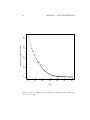
Box plots of queue lengths. 1) 10,000 ticks. 2) 20,000 ticks. .
MasterSetup #3. Nested for loops for a factorial data collection. . . . . . . . . . . . . . . . . . . . . . . . . . . . . . . .
Excel PivotTable report; data generated from MasterSetup #3
Queue length increases rapidly at 1000 ticks when arrival rate
exceeds service rate . . . . . . . . . . . . . . . . . . . . . . . .
78
9.3
9.4
vii
.
.
.
.
.
.
.
.
.
.
.
.
.
.
.
.
.
.
.
.
.
.
.
.
.
.
.
.
80
83
86
viii
Preface
Assumptions:
• Previous exposure to NetLogo models. Previous exposure to programming. In either case exposure can be quite minimal.
• Working with an open, new NetLogo model. Version: 5.X. These notes
separately.
• Here, highlights only. These tutorials are just a beginning, to get you
started and to serve as notes and as a quick reference.
• RTFM principle: read the manual, from NetLogo. Most important:
Programming Guide and NetLogo Dictionary. Read the Programming
Guide. Keep the NetLogo Dictionary to hand as you write code and
refer to it often. You can often find commands that will do exactly
what you need. But there are a lot of commands. Notice that they
are organized by category; see the top of the NetLogo Dictionary.
NetLogo demonstration files, written by me, can generally be downloaded (if available) at http://opim.wharton.upenn.edu/~sok/mandms/
nlogocode/ or perhaps more likely at http://opim.wharton.upenn.edu/
~sok/age/nlogo.
There isn’t much in the way of a NetLogo textbook or instruction manual
at all, other than what is present on the NetLogo Web site—
• NetLogo home page: http://ccl.northwestern.edu/netlogo/.
• NetLogo user manual: http://ccl.northwestern.edu/netlogo/docs/.
Note well: The user manual comes with three tutorials. I recommend
them, especially for beginners. Also, NetLogo comes with a models
library (under the File menu), which is full of interesting examples,
including code examples. Well worth rooting around in.
ix
—which is pretty good. NetLogo programmers should expect to consult it
regularly, especially the dictionary (see the user manual). Also, see the programming examples that come with NetLogo. They are extensive and quite
comprehensive. Recently, however, Agent-Based and Individual-Based Modeling [Railsback and Grimm, 2012] has appeared. It is excellent, if lengthy.
I highly recommend it for going beyond these Notes.
Probably
should
We use R, too, not just NetLogo. The home page for R is http://www.
switch to Python.
r-project.org/. You will find there, besides opportunity to download a
free copy of R, manuals and documentation. The newbie should start (and
probably finish) with An Introduction to R, which you can find online at
http://cran.r-project.org/doc/manuals/R-intro.html.
This booklet is very much a work in progress. It is aimed at helping
people new to NetLogo and with minimal programming experience get up
and running very quickly. Also, I’m trying to build up enough examples
that the booklet can be used as a reference work.
Comments and suggestions are most welcome and will be gratefully received.
For a quick start, see QuickStart.nlogo, with answers in QuickStartSolutions.nlogo.
x
Chapter 1
Starters
1.1
Starters
First of all, remember that NetLogo has a manual with lots of valuable
information. RTFM! For purposes of getting started you might consider
looking here and in the NetLogo manual. Here, begin immediately below. In
the NetLogo manual, begin with “Introduction” then move on to “Learning
NetLogo”. Skim the “Interface Guide” and the “Programming Guide” and
be prepared to consult them as you progress. The “NetLogo Dictionary” is
especially useful on a day-to-day basis.
1.1.1
NetLogo world view (main metaphors)
The NetLogo program/application has a main window with three tabs, for
three different functions:
Interface
Info
Code
The principal metaphors in NetLogo are these:
• From the manual:
The NetLogo world is made up of agents. Agents are beings
that can follow instructions. Each agent can carry out its
own activity, all simultaneously.
In NetLogo, there are four types of agents: turtles, patches,
links, and the observer. Turtles are agents that move around
in the world. The world is two dimensional and is divided
up into a grid of patches. Each patch is a square piece of
1
2
CHAPTER 1. STARTERS
“ground” over which turtles can move. Links are agents that
connect two turtles. The observer doesn’t have a location –
you can imagine it as looking out over the world of turtles
and patches.
• The world: rectangular array of patches on which turtles may sit.
Patches are (like) geographic locations and are fixed. Turtles are
moveable entities. Both have properties. In addition, turtles may
be connected by links, which are also agents.
• The observer: looks down at the world and what is in it.
From the Command Center. From the Procedures.
• The View. A window onto the world of patches and turtles. By default,
a black window on the Interface Tab.
We’ll focus next on the Interface Tab.
1.2
The Interface Tab
1.2.1
The Observer
• Again: The observer: looks down at the world and what is in it.
Can issue commands, from the Command Center. For example,
observer> create-turtles 1 creates a turtle at patch (0,0) or patch
0 0 as it is called in NetLogo.
Note: every patch has a planar or x-y coordinate address, measured
away from 0 0 in the cartesian plane.
observer> ask turtle 0 [fd 12] moves our turtle (ID is 0) forward
12 patches.
observer> ask turtle 0 [forward -12] puts it back at the origin.
1.2.2
Inspecting
• Right-click on the turtle. Investigate: inspect patch 0 0 and turtle
0. Inspect each. Note the properties of each.
Try observer> ask patch 2 2 [set pcolor red], and
observer> ask turtle 0 [set label "My first turtle!"].
1.2. THE INTERFACE TAB
3
Notice how NetLogo makes assignments to variables (and properties):
set <thing> <to value>.
Try observer> print count patches
and observer> print count turtles.
Now start over: observer> clear-all.
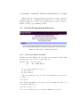
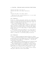
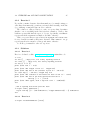
1.2.3
Editing the View (and the World)
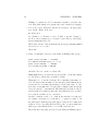
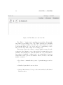
• Click on Edit... in the View window.
You get (by default) the window/dialog box shown in Figure 1.1, page
4.
4
CHAPTER 1. STARTERS
Figure 1.1: World & View Edit Dialog Box
1.2. THE INTERFACE TAB
1.2.4
5
More on Editing the World
• You control the size of the world—the number of patches—here.
Notice the coordinate system (by default): in horizontally and vertically symmetrical offsets from patch 0 0. The boundaries of the
world always have an odd number of patches.
By default, the world is a torus: it wraps horizontally and vertically.
You can modify that here.
If you want to create a world with very many patches, you will probably
also want to reduce the patch size (in pixels), which is done in the View
section of this dialog box.
1.2.5
Interface Widgets (on the Toolbar)
NetLogo has icons on the Toolbar for interface widgets.
Click and draw. Right-click to edit.
There are nine types (see the manual):
1. button
2. slider
3. switch
4. chooser
5. input
6. monitor
7. plot
8. output
9. note
1.2.5.1
NetLogo Interface Tab: The Interface Toolbar: Buttons
• Button: “Buttons can be either once-only buttons or forever buttons.
When you click on a once button, it executes its instructions once.
The forever button executes the instructions over and over, until you
click on the button again to stop the action.”
Click and draw a button. In the “Commands” text area put:
6
CHAPTER 1. STARTERS
print Mutation?
if-else (Mutation?)
[set Mutation? false]
[set Mutation? true]
Accept and try it out.
1.2.5.2
NetLogo Interface Tab: The Interface Toolbar: Sliders
• Slider: “Sliders are global variables, which are accessible by all agents.
They are used in models as a quick way to change a variable without
having to recode the procedure every time. Instead, the user moves
the slider to a value and observes what happens in the model.”
Click and draw a slider. Set “Global variable” to myFirstVariable,
leave “Minimum” at 0, set “Increment” to 0.1, “Maximum” to 10, and
“Value” to 7.3. Click “OK”. Move the slider to a new value.
Try observer> print Myfirstvariable. (We see that NetLogo is
not case-senstive.) Try observer> set myFirstVariable 9.9
then observer> set myFirstVariable 29,
and then observer> print myFirstVariable.
Note well
Note well: Starting in version 4, NetLogo allows you to change slider
variables to values outside those declared in the slider. I’m not sure this is
an improvement, but there you have it. So, you can’t rely on there being a
maximum or minimum value to a slider variable. You will need to program
them yourself.
1.2.5.3
NetLogo Interface Tab: The Interface Toolbar: Switches
• Switch: “Switches are a visual representation for a true/false variable.
The user is asked to set the variable to either on (true) or off (false)
by flipping the switch.”
Click and draw a switch. Set “Global variable” to Mutation?. Toggle
the switch and try observer> print Mutation?.
• Sliders, switches and choosers are the only interface widgets available
for sending information from the user interface to the Observer (or
NetLogo procedures).
1.2. THE INTERFACE TAB
1.2.5.4
7
The Interface Toolbar: Choosers
• Chooser: “Choosers let the user choose a value for a global variable
from a list of choices, presented in a drop down menu.”
One per line. Put strings in double quotes. Numbers directly.
Click and draw a chooser. In the “Global variable” text area, type
person. In the “Choices” text area type:
"Bob"
"Carol"
"Ted"
"Alice"
9
23.34
Accept and try it out. Note: Choosers don’t accept functions to evaluate. (Choosers can’t be beggars?)
Right-click on the monitor and choose “Edit”. Insert person as the
global variable. Accept and try it out.
Comment: You can also use a chooser to control execution of the
program. Think of the choices as determining scenarios.
1.2.5.5
The Interface Toolbar: Input boxes
• Input: “Input Boxes are global variables that contain strings or numbers. The model author chooses what types of values the user can
enter. Input boxes can be set to check the syntax of a string for commands or reporters. Number input boxes read any type of constant
number expression which allows a more open way to express numbers
than a slider. Color input boxes offer a NetLogo color chooser to the
user.”
• Try one out. Use the variable name bob. Type print bob from the
command center.
1.2.5.6
The Interface Toolbar: Monitor
• Monitor: “Monitors display the value of any expression. The expression could be a variable, a complex expression, or a call to a reporter.
Monitors automatically update several times per second.”
8
CHAPTER 1. STARTERS
A reporter is a procedure that returns a value. We’re not there yet
(but we will be).
Click and draw a monitor. In the “Reporter” text area, type Mutation?.
Accept and try it out.
1.2.5.7
The Interface Toolbar: Plot
See §1.2.6 below, page 8.
1.2.5.8
The Interface Toolbar: Output
• Output: “The output area is a scrolling area of text which can be used
to create a log of activity in the model. A model may only have one
output area.”
Click and draw an output area. Edit the button and change the first
line from print Mutation? to output-print Mutation?.
Accept and try it out. You can essentially achieve this by writing to
the Command Center with print etc. However, clear-all clears the
output area, but not the command center output area.
See also: print, show, type, write.
1.2.5.9
The Interface Toolbar: Note
• Note: “Notes lets [sic] you add informative text labels to the Interface
tab. The contents of notes do not change as the model runs.”
Nor can your program modify them. Useful for giving basic directions
to users.
Click and draw a note. Insert “Click here to initialize:” in the text
area. Accept. Right-click and choose “Select”. Move (mouse down
and drag) the note to a point above the button. Click outside the note
to deselect it.
1.2.6
The Interface Toolbar: Plot
We’re going to create a stream (eventually two streams) random walk data,
and plot the results. This will be a bit more complex than what we have
done so far.
1. Begin by creating two buttons: Setup and Random Walking. For now,
just give them display names only, with nothing to do.
1.2. THE INTERFACE TAB
9
2. Create a slider whose global variable is daNewA. Set the minimum to
-1, the increment to 0.000001, the maximum to 1, and the value to
0.1.
Note: Setting the increment to 0.000001 or 1.0E-6 (or some similarly small value) is crucial. If you set it too high, say to 0.1, then
I get unusual and implausible numbers set via the random number
generator.
3. Create a slider whose global variable is streamA. Set the minimum to
0, the increment to 1.0E-5, the maximum to 50, and the value to 30.
4. In the “Commands” text area of the Setup button, type:
clear-all
set daNewA 0.0
set streamA 25.0
random-seed 1
Accept and click the button. The two slider values should change.
This button now: (1) reinitializes the system (clears the World, clears
the plots). (2) Sets the global variable daNewA to have the value 0.0.
(3) Sets the global variable streamA to have the value 25.0. And, (4),
initializes the random number generator using the seed 1.
Comment on random number generators: They play an absolutely
critical role in simulations and experimental mathematics, such as we
are doing. They are, however, only pseudo-random. In fact, given a
starting seed value, they are absolutely deterministic and eventually
they cycle! The thing that unless you know the generator, just looking
at its stream of random numbers you can’t tell (ideally that is), that
they aren’t being generated from an ideal random number generator.
If you don’t set the seed, NetLogo uses the system clock, so on each
run you will see a different random number stream. It is useful when
you are developing a model to set the random number seed yourself,
since that will produce predictable output. When you are exploring
your model, after it is developed, you should explore using multiple
random seeds, either by letting NetLogo pick them or by explicitly
setting them yourself.
It is typical in NetLogo models to have a setup button that initializes the system and a second button—ours here is called “Random
10
CHAPTER 1. STARTERS
Walking”–to run the model. You may find it useful to add other buttons. Especially during development, they can be useful for debugging.
5. Now create a plot. Click and drag the plot widget to an appropriate
spot. In the “Name” field, type:
My first plot
Set “X min” to 0, “X max” to 10.0, “Y min” to 20, and “Y max” to
30. Note: these settings are not crucial, because NetLogo will change
them dynamically as needed.
Click on the “Create” button and name the new plot pen daStreamAPen.
Select its color to be cyan.
Click “Ok”.
6. In the “Commands” text area of the Random Walking button, type:
print (word "streamA " streamA)
set daNewA ((random-float 1) - 0.5)
print (word "daNewA " daNewA)
set streamA (streamA + daNewA)
Click the “Forever” check box. Click “Ok”.
Note well: NetLogo now uses the reporter word to concatenate strings.
See the NetLogo Dictionary on word for details.
What this code does is the following. We’ve initialized streamA to be
25.0. We draw a random number between 0 and 1 (with random-float
1) and add it to streamA, subtracting 0.5 at the same time. So, the
new value of streamA is the old value plus or minus a random amount
between 0 and 0.5. streamA will drift aimlessly, in what is called a
random walk. Note that step intervals other than (0, 0.5) are possible;
we’ve just chosen that one for convenience.
Another comment on the code. word in the first line is being used
as a string concatenator (“concatenator” = “putter together”). In
the third and fourth lines the plus sign is being used for numerical
addition. Notice especially that in NetLogo the operators must have
white space surrounding them. a + b is OK, but a+b is not.
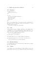
Then click the Setup button followed by the Random Walking button.
1.2. THE INTERFACE TAB
11
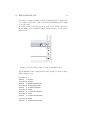
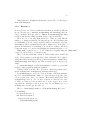
You will see output scrolling by in the Command Center output window. After a short time, click on the Random Walking button again
to stop the run.
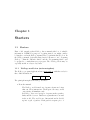
Now click on the double-headed arrow, next to the “Clear” button, at
the far right of the Command Center output window. See the image
that follows.
Figure 1.2: Double-Headed Arrow of the Command Center
The Command Center output window will expand for easier viewing.
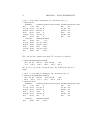
This is what you get:
streamA
daNewA
streamA
daNewA
streamA
daNewA
streamA
daNewA
streamA
daNewA
streamA
daNewA
25.0
-0.082978
24.917022
-0.4998856316786342
24.417136368321366
-0.353244107423887
24.06389
-0.3137397857321689
23.75015
-0.10323251879902084
23.64692
-0.08080549071321619
12
CHAPTER 1. STARTERS
streamA
daNewA
streamA
daNewA
streamA
daNewA
streamA
23.566114509286784
-0.295548
23.270561999999998
-0.47261240282038
22.79795
-0.08269519422643179
22.71525480577357
Note again: Seeding the random number generator with 1 should produce these values reliably. (Actually, sometimes NetLogo seems to
round off the values. I’m not clear why this seemingly irregular behavior occurs.)
Click the Clear button to remove the text from the Command Center
window. Click the double-headed arrow again to return the Command
Center window to its original and diminished position.
7. Now let’s do some plotting. Add the following code to the code area
of the Random Walking button:
set-current-plot "My first plot"
set-current-plot-pen "daStreamAPen"
plot-pen-down
plot streamA
This snippet of code should be readily understandable. First, we tell
NetLogo which (of possibly many) plots we want to access. Next we
tell NetLogo which (of possibly many) pens (for distinct streams of
data) we wish to use. We place the pen down and we plot the current
value of our variable of interest, here streamA. And that’s it.
Click the Ok button in the Random Walking dialog box. Click the
Setup button, then click Random Walking and watch the plot unfold!
8. Now we’ll add a second random walk stream. First, add two new
sliders, for global variables daNewB and streamB, analogous to daNewA
and streamA. Second, edit (right-click then choose “Edit”) your plot,
creating a new pen called daStreamBPen and set its color to magenta.
Third, modify the code for the Setup button to read as follows:
clear-all
1.2. THE INTERFACE TAB
13
set daNewA 0.0
set streamA 25.0
set daNewB 0.0
set streamB 25.0
random-seed 1
And fourth, modify the code for the Random Walking button to read
as follows:
;print (word "streamA " streamA)
set daNewA ((random-float 1) - 0.5)
;print (word "daNewA " daNewA)
set streamA (streamA + daNewA)
set daNewB ((random-float 1) - 0.5)
set streamB (streamB + daNewB)
set-current-plot "My first plot"
set-current-plot-pen "daStreamAPen"
plot-pen-down
plot streamA
set-current-plot-pen "daStreamBPen"
plot-pen-down
plot streamB
Note that lines 1 and 3 now begin with a semicolon – ; – which is the
NetLogo comment symbol. Presumably we don’t need to print out the
values anymore. Commenting out the lines serves the useful purpose
of reminding us of what we did and allows us to quickly remove the
comments if we want to regain the lines of code. Even better would be
to comment profusely, as in this tutorial, but in the code itself, using
comment lines.
9. Experiment!
How long does it take the streams to cross over? Try a different random
number seed. What happens?
1.2.7
Introduce a Bug
The first line of the code for the Random Walking button is now
;print (word "streamA " streamA)
Change it to
14
CHAPTER 1. STARTERS
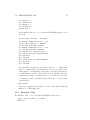
print "streamA " streamA
That is, remove the semicolon, the parentheses, and word.
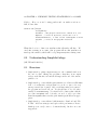
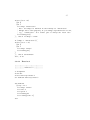
Click the Ok button. Notice that we return to the Interface Tab but the
lettering on the Random Walking button is now in red. This indicates an
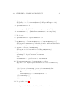
error. Edit the button. Here is what you will see:
Figure 1.3: NetLogo Error Message from a Button
The cursor will also be on the offending line. Fix it.
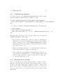
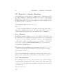
1.3
The Info Tab
Not a lot to say here. A nice design. Two modes: view and edit. Go to edit
mode and notice the simple pattern.
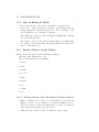
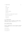
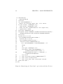
[Later: Using the ODD protocol here for documentation: http://bio.
uib.no/te/papers/Grimm_2010_The_ODD_protocol_.pdf.
1. Purpose
2. State variables and scales
1.4. THE CODE TAB
15
3. Process overview and scheduling
4. Design concepts
5. Initialization
6. Input
7. Submodels
See also nice discussion in Agent-Based and Individual-Based Modeling by
Railsback and Grimm.]
Add in—
EXTRA STUFF
----------You can add categories of your own.
—and return to view mode.
Notice that full URLs are “live,” e.g., try inserting http://opim-sky.
wharton.upenn.edu/~sok/.
Also, vertical bars at the beginning of lines indicate special shading for
emphasis, e.g., to present code.
|
|
|
|
|
|
clear-all
set daNewA 0.0
set streamA 25.0
set daNewB 0.0
set streamB 25.0
random-seed 1
Notice that the shaded area uses “typewriter” font (conventional for code).
1.4
The Code Tab
We can do a great deal of NetLogo programming by proceeding as we have,
adding code to buttons on the Interface Tab. This quickly becomes a software engineering nightmare, however. The Procedures Tab helps us avoid,
or at least postpone, this unhappy eventuality.
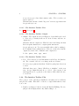
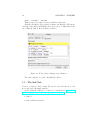
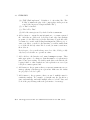
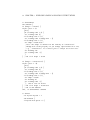
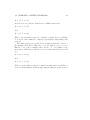
Open a new (blank) NetLogo file and click on the Procedures Tab. Here’s
what you see (and get):
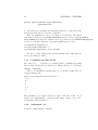
16
CHAPTER 1. STARTERS
Figure 1.4: The Window for the Code Tab
The “Find. . . ” function is for searching for text in the edit area (the
large white area extending below). The “Check” function is for validating
your code, looking for syntax errors. The “Procedures” function is a dropdown list that allows you to see, select, and go to a particular procedure.
The rest is the large white editing area extending below.
There are two types of procedures: commands (which correspond to subroutines in other languages or procedures with void returns) and reporters
(which in other languages are often called functions, or procedures that return values). Commands do things, but do not return values. Reporters
return values. NetLogo is not case-sensitive. Even so, I’ll try to follow this
stylistic convention:
• Procedures—commands and reporters—begin with an upper-case letter
• Variables begin with a lower-case letter
• After the first character, both procedures and variables UseTheCamelBackConvention.
1.4. THE CODE TAB
1.4.1
17
Commands and reporters
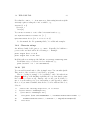
To declare a reporter, call it SumOfTwoNumsSquared, that accepts one argument and returns the argument plus one squared, do this:
to-report SumOfTwoNumsSquared [daFirstNumber daSecondNumber]
report (daFirstNumber + daSecondNumber) * (daFirstNumber + daSecondNumber)
end
To declare a command, call it MyFirstCommand, use the following format:
to MyFirstCommand
print "Hello from MyFirstCommand."
print (word "The square of 3 + 2 is "
end
SumOfTwoNumsSquared(3)(2)
Try typing these into the procedures edit area. Then create a button and
call MyFirstCommand. Points arising:
1. Reporters and commands may or may not require accompanying arguments to be specified. If arguments are specified you show this as
in the declaration for the reporter SumOfTwoNumsSquared, with the
arguments specified between square brackets and separated by white
space if there is more one.
2. NetLogo uses square brackets, [. . . ], to indicate lists (of which more
later). Items in a list are separated by white space.
3. NetLogo supports various arithmetic and mathematical operators, e.g.,
+ for addition, * for multiplication, ^ for exponentiation, and so forth.
NetLogo requires that these operators be surrounded by white space.
So, 2*3 is not legal, but 2 * 3 is.
1.4.2
Global and local variables
NetLogo’s variables are not typed, but they must be declared. NetLogo
supports both global and local variables. Global variables may be declared
in either of two ways. First, using a variable in a slider or switch on the
Interface Tab counts as declaring the variable as global. Second, at the top
of the procedures edit area, you can declare NetLogo global variables using
this format:
".")
18
CHAPTER 1. STARTERS
globals [myFirstVariable mySecondVariable
myThirdVariable
]
So, the notation for declaring global variables in the Procedures Tab is the
keyword globals followed by a list of variables.
There are similarly two ways of declaring local variables. The first is
demonstrated in the reporter SumOfTwoNumsSquared, above. There, [daFirstNumber
daSecondNumber] declares two variables whose scope is the reporter SumOfTwoNumsSquared.
Second, you can place this sort of expression within any procedure:
let myFirstLocalVariable 0
let mySecondLocalVariable ""
let myThirdLocalVariable one-of patches
Use let to declare variables and give them initial values. Thereafter use
set to give them new values.
1.4.3
Comments and line breaks
The semicolon— ; —is NetLogo’s comment symbol. Anything appearing
after a semicolon in a line is considered a comment. NetLogo does not have
multiline commenting.
NetLogo is remarkably forgiving and loose about line breaks. The following is entirely OK:
print (word "Sum from several lines: "
( 3 +
4 3
+
1 )
)
The parentheses are required, but not because of the line breaks. If you
want to use mathematical operators in this string context, you need to
group things with parentheses.
1.4.4
Assignment: Set
Use Set to assign values to variables.
1.4. THE CODE TAB
19
Set myFirstVariable 17.2
Variables may hold complex objects, including lists, turtles and patches.
Just use Set.
1.4.5
Agent properties, turtles-own, and patches-own
Turtles and patches are agents, objects with properties. By default every
patch has the properties: pxcor, pycor (its x and y coordinates on the
world grid), pcolor (its color), plabel, and plabel-color. You can see
the properties of a patch by right-clicking on it, then choosing to inspect it.
Turtles come by default with a longer list of properties. These, too, you can
see (and edit) by right-clicking on a turtle and choosing to inspect it.
Your program can alter any properties a patch or turtle has. In addition,
and most usefully, your program can add properties to turtles and to patches.
For example, placing
patches-own [ playerType ]
at the beginning of the procedures edit area, below globals and above the
first procedure will cause all patches to have a new property, playerType.
If you want more properties added, just add them to the list, which above
contains just playerType. Similarly, you can add properties to turtles with,
e.g.,
turtles-own [ speed availableEnergy]
If you want to set a property of a turtle or patch to a certain value, you
ask, e.g.,
ask turtle 0 [set shape "airplane"]
Note: every turtle has an ID number. Numbering is in sequence, beginning
with 0. There are a number of shapes that ship with NetLogo (ship shapes?).
You can see the current list by typing
show shapes
in the Command Center. Similarly, you can ask a patch to set one of its
properties, whether given by default or added by you, e.g.,
ask patch
1 2 [set playerType "type01"]
20
CHAPTER 1. STARTERS
Note that every patch is identified uniquely by its x-y coordinate numbers
on the world grid.
If you want all the patches or turtles to do something, you just ask, e.g.,
ask patches [set pcolor "blue"]
And similarly for ask turtles. With these commands you exploit NetLogo’s simulation of parallel programming. NetLogo updates the agents in
random order.
NetLogo’s of and one-of mechanisms are also quite useful. -of is used
with a property, e.g.
set [color] of turtle 0 blue
Use of when dealing with one turtle or one patch. You can also use it for
agentsets, collections of NetLogo agents (see §1.4.6 below). See of in the
Dictionary.
You use with to select a set of turtles or patches from a larger group,
e.g.,
ask turtles with [shape = "default"] [set color green]
Again, see the Dictionary.
NetLogo’s one-of randomly selects one item from a list. For example,
print one-of ["Bob" "Carol" "Ted" "Alice"]
1.4.6
Agentsets
See the discussion in the NetLogo manual. An agentset is a set of patches
or a set of turtles. Agentsets are unordered. They are a fundamental and
crucial concept in NetLogo. The turtles built-in primitive is a reporter
that reports the agentset of all turtles presently in the model. Similarly for
patches. Great power of expression comes from the fact that agentsets can
be given as arguments to reporters, which then operate on them, and the
fact that agentsets may be composed or defined under program control, for
example by filtering another agentset. Examples:
count patches applies the count reporter to the patches agentset.
print count turtles with [color = green] filters the agentset turtles,
creating a new agentset of green turtles, then applies the count reporter to
this.
See additional examples on page 81 of the manual. Useful agentset constructors:
1.4. THE CODE TAB
21
• with
• turtles-here
• in-radius
• at-points
• neighbors4, neighbors
• turtles-on
Useful built-in reporters taking agentsets as arguments:
• max-one-of and min-one-of
• one-of, n-of
• values-from
1.4.7
Breeds of turtles
Turtles, but not patches, can be organized by breeds, which are classes—
distinct agentsets—of turtles. Use breed at the top of the procedures edit
area, before the procedures, to declare new breeds, e.g.,
breed [ optimists optimist]
breed [ pessimists pessimist]
Then, where you might say turtles you can now say optimists or pessimists,
and where you might say turtle you can now say optimist or pessimist.
You can still write
create-turtles 17
and you can also write
create-optimists 23
22
1.4.8
CHAPTER 1. STARTERS
Lists
Lists are ordered collections of things and may be heterogeneous, e.g.,
print (list "Bob" 5 [2 "Carol"] turtle 0)
prints out [Bob 5 [2 Carol] (turtle 0)].
If you have more than 2 things to put into the list you must use parentheses in creating it (see above).
There are several built-in reporters that can be used to change a list.
Examples:
set daList replace-item 3 daList (list 1 2 3)
This replaces whatever item 3 was (the fourth item, since we count starting
at 0) with [1 2 3].
set daList fput "Bob" daList
Note well
This adds "Bob" to the beginning (position 0) of daList, making it one item
longer. Use lput for adding to the end. Note well: In NetLogo lists are
naturally accessed from the front. If you need to access (add, delete, find
something in) a list towards the end, it will often be faster to reverse the
list, access it, and then reverse it again.
set daList but-first daList
This removes the first item in daList. Use but-last to remove the last
item.
List are used for controlling iteration. Example:
foreach [1 2 3]
[crt ?]
This does what in other languages might be done with
for i=1 to 3
crt(i)
next i
or with
for (int i=1; i < 4; i++) {
crt(i)
}
1.4. THE CODE TAB
23
Note that the counter— ? —is anonymous, so that nesting interations (with
foreach) requires reading the ? into a variable, e.g.,
foreach [1 2 3]
[set myi ?
crt myi]
You can use n-values to create a list for foreach iteration, e.g.,
set myIterationList n-values 10 [ ? ]
myIterationList is now [0 1 2 3 4 5 6 7 8 9].
See the manual, the “Programming Guide,” for additional examples.
1.4.9
Character strings
Are indicated with double quotes, e.g., "Bob". Generally, if a built-in reporter works on a list it will work on a string, too. Example:
print length (list 2 4 6 8)
print length "Now is the time"
In addition there are string-specific built-ins: is-string?, substring, word.
Recall that string concatenation is done with word, e.g.,
print (word 17 " is " "an odd number").
1.4.10
I/O
You can read from and write to files, in simple ways. You can make QuickTime movies of the execution of your NetLogo program.
Here, too briefly, is example code for writing to a file. It’s taken from
Chapter 9. NetLogo’s file handling capabilities are very basic (maybe primitive would be a better word). Anyway, only one file open at a time, be
sure to close files when you’re done, and writing to a file appends to what’s
there, so if you want a blank file, first check to see if it exists and if it does,
delete it.
4
5
6
18
19
20
; Delete the existing output file, if it exists.
if file-exists? "runsOutput.txt"
[file-delete "runsOutput.txt"]
file-print (word currentRunNumber "," meanCustomerInterarrivalTime ","
meanCustomerServiceTime "," maxTicks "," length(customerQueue))
file-close
24
CHAPTER 1. STARTERS
1.4.11
Control flow and logic
See Control/Logic in the NetLogo Dictionary. Main ones:
1. foreach From the manual:
foreach [1.1 2.2 2.6] [ show (word ? " -> " round ?) ]
=> 1.1 -> 1
=> 2.2 -> 2
=> 2.6 -> 3
Issues: (a) use of ?; getting a list. On the latter, see n-values. From
the manual:
show n-values 5 [1]
=> [1 1 1 1 1]
show n-values 5 [?]
=> [0 1 2 3 4]
show n-values 3 [turtle ?]
=> [(turtle 0) (turtle 1) (turtle 2)]
show n-values 5 [? * ?]
=> [0 1 4 9 16]
2. if and ifelse
From the manual:
ifelse reporter [ commands1 ] [ commands2 ]
Reporter must report a boolean (true or false) value.
If reporter reports true, runs commands1.
If reporter reports false, runs commands2.
ask patches
[ ifelse pxcor > 0
[ set pcolor blue ]
[ set pcolor red ] ]
;; the left half of the world turns red and
;; the right half turns blue
1.4. THE CODE TAB
25
3. while
From the manual:
while [reporter] [ commands ]
If reporter reports false, exit the loop. Otherwise run commands and repeat.
The reporter may have different values for different agents,
so some agents may run commands a different number of times
than other agents.
while [any? other turtles-here]
[ fd 1 ]
;; turtle moves until it finds a patch that has
;; no other turtles on it
1.4.12
Typical program structure
Two main command procedures: Setup and (then) Go, both called by buttons on the Interface tab, and Go a forever button. Setup initializes, Go
handles the main loop of execution. Both can (and usually should) call
various reporters and command procedures as subroutines.
26
CHAPTER 1. STARTERS
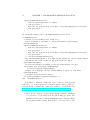
Chapter 2
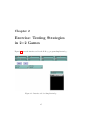
Exercise: Testing Strategies
in 2×2 Games
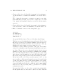
Figure 2.1 shows the interface tab for the NetLogo program Simple2x2.nlogo.
Figure 2.1: Interface tab for Simple2x2.nlogo
27
28 CHAPTER 2. EXERCISE: TESTING STRATEGIES IN 2×2 GAMES
This program is for testing strategies in iterated 2×2 games. Our aim
with this exercise is to understand how Simple2x2.nlogo works and then to
modify and improve it. Before we do that, however, we need to review a
number of NetLogo programming elements.
2.1
Needed Programming Elements
Figure 2.2: The NetLogo Dictionary. Use it!
2.1.1
Local and Global Variables
Variables set on the Interface tab are global, as are variables declared with
globals (at the top of the Procedures window).
globals [Row ; the row player
Col ; the column player
]
To set a global variable, use set, e.g.,
set Row turtle 0
set Col turtle 1
All other variables are local. To declare a local variable use let and give
it a value, e.g.,
let carol 8
Once declared (assuming you are in its scope) you change the value of a
local variable with set, e.g.,
set carol (carol + 1)
Note: you need white space before and after arithmetic operations.
2.1. NEEDED PROGRAMMING ELEMENTS
2.1.2
29
Reporters
to-report bob [x y]
report (list 3 4 x y)
end
to test
let carol bob ("hello")("there")
print first carol
print last carol
print carol
end
This code is in Simple2x2.nlogo. Try typing test in the command line (on
the interface tab). Note that using a test procedure like this is a good idea
during program development.
Note well: use of square and round brackets.
2.1.3
Lists
A list is just an sequence of things. In NetLogo, these things can be
. . . anything more or less, including numbers, strings, turtles and so on.
NetLogo uses square brackets to delineate lists: [bob carol ted alice].
Notice: spaces not commas separate the elements.
Note to create lists use list as in
let bob (list 2 3 4 5 "hello")
Note further this is how you do string building (concatentation):
let myString (word "Now is" " the time " "for all etc.")
Let’s look at the List category in the Dictionary. . . .
2.1.4
Random Numbers
See the Mathematical category in the Dictionary. random-float is perhaps
the most commonly used.
2.1.5
Turtles
See the Turtle category in the Dictionary. Turtles (which can move) and
patches (which cannot move) are, with lists, the main data structures in
30 CHAPTER 2. EXERCISE: TESTING STRATEGIES IN 2×2 GAMES
NetLogo. Here, we won’t be using patches and our turtles won’t move.
Still, we have this:
turtles-own [Player
PolicyOfPlay
NextMove ; the player’s next move, which is 0 or 1
MyMoves ; a list of my moves, moves are 0 or 1
CounterPartMoves ; a list of the counterpart’s moves
Payoffs ; a list of the payoffs received
]
What this does is to define new attributes that all turtles will have. We
can define as many as we want. Our program will use this attributes as
turtle-specific variables, which will be set perhaps many times during a run.
2.2
Understanding Simple2x2.nlogo
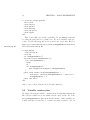
[OK, I’ll handle this live.]
2.3
Exercises
1. Simple2x2.nlogo prints output messages to the command window at
the end of a run. Change the program so that there is an output
widget on the Interface tab and the messages at the end of the run are
printed to it.
2. Simple2x2.nlogo comes with the game matrix set to a Prisoner’s Dilemma.
Add code an Interface widgets that let you choose (use a chooser)
among a stated list of games. Add several interesting 2×2 games to
the program and test it all out. You should have a chooser whose
variable is PickGameSetup. You should add a button that calls the
procedure SetUpGame and, obviously, you need to add a procedure
named SetUpGame that resets the game matrix payoff sliders as appropriate.
3. Simple2x2.nlogo comes with two built-in straties: “Random” and “TitForTat”. Add new strategies and explore their performances. Best to
think up your own (be sure to document them!), but here are some
suggestions.
2.3. EXERCISES
31
(a) “TitForTatComplement”. Defaults to 1, after that, like “TitForTat” it mimics the play of the counter-player in the previous
round. (Also known as “SuspiciousTitForTat”.)
(b) “2 Tits for OneTat”.
(c) “Tit for Two Tats”.
(d) All of the strategies used by Axelrod in his tournaments.
4. Add a feature to output the run information to a comma separated
file. Such files are easily read by R, Excel, and other data analysis
programs. See the Files category in the Dictionary. You should settle
on a name for your file, such as Simple2x2Output.txt. When you go to
write your data to your file for the first time, you will normally want
to see if the file already exists. If it does and you want to start anew,
then delete it.
Don’t forget to close your file when you are done. Also, NetLogo really
only lets you deal with one open file at a time.
5. Add a slider to the Interface tab, named NumReplications. Then
make appropriate code changes so that that number of replications is
run for any given setting. Preferably, make this work with the file
logging feature so that results from each replication are stored (as
rows) in a comma separated file.
6. Add features to the program so that you can run tournaments, say one
strategy playing each strategy in a given list. Make sure the results
are properly recorded a log file.
7. Add features to the program so that you can do multiple runs for
sensitivity analysis. For example, you might vary the payoffs in a
game systematically, undertake multiple runs, record the data, and
see how the payoff changes affect the performance of a strategy.
$Id: strategy-tester-2x2.tex 3684 2013-09-09 20:37:28Z sok $
32 CHAPTER 2. EXERCISE: TESTING STRATEGIES IN 2×2 GAMES
Chapter 3
Exercise: Simple animation
with turtles
In this exercise, or series of exercises, we will have one or more trucks move
between two points, which we might think of as notional supply and delivery
locations.
Since the trucks have to move, we use turtles to embody them. NetLogo
comes, I shall assume, with a truck shape. Verify this by choosing Turtle
Shapes Editor under the Tools menu in NetLogo. You should find a scrolling
window displaying turtle shapes, with truck near the bottom. Note that you
can also click on Import from Library. . . and see an even larger collection
of turtle shapes. Select (click on) truck, then click on Duplicate. In the
new window, type truck-west to name our new shape. Then click Flip
Horizontal to head the truck to the west (left). Click OK. You should now
see your new shape in the Shapes Editor scrolling window. Click the go-away
button on the window and return to the main window of NetLogo.
Why did we do this? Our trucks will start in the west and head east
to a specified point. After that, they will turn around and head west to a
specified point, and so on. The truck shape is not symmetric, so rotating it
(which is all NetLogo can do under program control) won’t make it point
west without being upside down. (Notice that in the Shapes Editor, the
Rotatable check box is unchecked. You can check it and thereby allow your
program to rotate the truck—e.g., with right or rt—but why would you
want an upside-down truck?) So, we will use two shapes with the same
turtle.
In the command center, test things out with:
observer> crt 1
33
34 CHAPTER 3. EXERCISE: SIMPLE ANIMATION WITH TURTLES
observer> ask turtle 0 [set size 4]
observer> ask turtle 0 [set shape "truck-west"]
then
observer> ask turtle 0 [set shape "truck"]
OK. Now we’ll do three exercises in which we move one or more trucks
back and forth across the gridscape.
3.0.1
Exercise 1
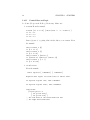
We write two commands: Setup and Go. In Setup, create a single turtle,
and give it a name, say daTruck which should be global. Position the truck
at patch -10 0. Hint: Use setxy. Give the truck the shape "truck", set
its size to 4, and its heading to 90 (due east).
In Go, when the truck has the shape "truck" move it forward east
one patch per run of Go, until the truck is on patch 10 0. Then, set the
shape to "truck-west" and the heading to 270 (due west). If the shape is
"truck-west", move the truck forward west one patch at a time, until the
truck is on patch -10 0. Now, change its shape to "truck" again and its
heading to due east.
Create buttons for Setup and Go, making Go a forever button. Exercise
the code. Use the speed control slider at the top of the world window to
control the speed of the truck. Experiment with the code a bit to add
features, e.g., change the color of the truck depending on its direction.
3.0.2
Exercise 2
We write two commands: SetupPlus and GoPlus, and buttons to call them.
Now we declare delivery-trucks as a new breed with breed [delivery-trucks
delivery-truck] and we add loading-time as a property of delivery-trucks.
Do this with delivery-trucks-own [ loading-time ]. Our truck will
take some time to load and unload.
Write SetupPlus much as you did Setup, but use create-delivery-trucks
instead of create-turtles and set the loading-time of our truck to -1.
Write GoTruckPlus much as you did GoTruck, but when the truck arrives at the eastern terminus, set its loading-time to 4, then decrement
loading-time by 1 each time step until it equals 0. At that time, set the
shape and direction for heading west, and set loading-time to -1 again.
When the truck arrives at the western terminus, it should be handled
analogously to what was done at the eastern terminus.
35
Using buttons for SetupPlus and GoPlus, exercise the code and experiment with changing it.
3.0.3
Exercise 3
Now we’ll create two delivery trucks and run them in parallel at different
speeds. We write two commands: SetupPlusArg and GoPlusArg, and buttons to call them. We’ll also write a command, GoTruckPlusArg that takes
a delivery truck as its calling argument and processes its activities.
There are one or two important issues here. First, we want different
trucks to do things at different, idiosyncratic speeds. We’ll facilitate this
by maintaining a global counter, mytick, which we increment each time
GoPlusArg is called. A particular truck will do things based on the value of
mytick. A truck that does something every 2 ticks, for example, will check
for mytick mod 2 = 0. A slower truck might act when mytick mod 5 = 0.
Note well: Consider how to do all of this more elegantly using the Note well
reserved words in NetLogo, tick and ticks.
The second important issue is that we want a single way to handle all
of the delivery trucks, even though they behave differently. We do this by
giving them different values for their properties and writing a command (here
GoTruckPlusArg) that handles any delivery truck based on its property
values.
So, GoTruckPlusArg is very like GoTruckPlus of exercise 2, except that
it takes a delivery truck as an input argument.
Delivery trucks now have more properties: delivery-trucks-own [
speed loading-time loading-flag loading-time-left].
In SetupPlusArg we create two delivery trucks. Call them daTruck,
as before, and daOtherTruck. Make one of the truck green and the other
yellow (or pick some other color scheme). Both trucks should have their
loading-flag set at -1. Let one have a speed of 2 and give the other
3. Have one truck go between patch -10 0 on the west to 10 0 on the
east, while the other has a route from -10 10 to 10 10. Finally, give one a
loading-time of 3 and give the other a 5.
The job of GoPlusArg is mainly to call GoTruckPlusArg. Here it is:
to GoPlusArg
set mytick mytick + 1
ask delivery-trucks [
if mytick mod speed = 0
[GoTruckPlusArg(self)]
36 CHAPTER 3. EXERCISE: SIMPLE ANIMATION WITH TURTLES
]
end
The role of self is crucial in this quite elegant NetLogo approach to the
problem. ask delivery-trucks iterates in random order through the agentset
delivery-trucks. The agent it happens to be processing at a given time
is called self, which name we use as the argument to GoTruckPlusArg.
(Otherwise, how would we do this?)
Using buttons for SetupPlusArg and GoPlusArg, exercise the code and
experiment with changing it.
3.0.4
Solutions
The NetLogo program is animation-1-truck.nlogo. When all three exercises are implemented the leading declarations are:
globals [ daTruck mytick
daOtherTruck ]
breed [delivery-trucks delivery-truck]
delivery-trucks-own [ speed loading-time loading-flag loading-time-left]
3.0.4.1
Exercise 1
;;;;;;;;;;;;;;;;;;;;;;;;;;;;;;;;
;;;;;;;; Exercise 1 ;;;;;;;;;;;;
to Setup
clear-all
create-turtles 1
set daTruck turtle 0
ask daTruck
[setxy -10 0
set shape "truck"
set size 4
set heading 90]
end
to Go
ask daTruck [
if (shape = "truck") [
37
ifelse (xcor < 9)
[fd 1]
[fd 1
set shape "truck-west"
; Note: the shape is defined in the library as "truck-west"
; Things don’t work properly if you change capitalization at all,
; e.g., "truck-west". It’s safest just to always use lower case.
set heading 270]
] ; end of if shape = truck
if (shape = "truck-west") [
ifelse (xcor > -9)
[fd 1]
[fd 1
set shape "truck"
set heading 90]
]
] ; end of ask daTruck
end ; of Go
3.0.4.2
Exercise 2
;;;;;;;;;;;;;;;;;;;;;;;;;;;;;;;;;
;;;;;;;;;;; Exercise 2 ;;;;;;;;;;
to SetupPlus
clear-all
create-delivery-trucks 1
set daTruck delivery-truck 0
ask daTruck
[setxy -10 0
set shape "truck"
set size 4
set speed 3
set heading 90
set loading-time -1]
end
38 CHAPTER 3. EXERCISE: SIMPLE ANIMATION WITH TURTLES
to GoTruckPlus
ask daTruck [
if (shape = "truck") [
ifelse (xcor < 9)
[fd 1]
[if (loading-time < 0) [
set loading-time 4]
if (loading-time > 0) [
set loading-time loading-time - 1]
if (loading-time = 0) [
set shape "truck-west"
; Note: the shape is defined in the library as "truck-west"
; Things don’t work properly if you change capitalization at all,
; e.g., "truck-west". It’s safest just to always use lower case.
set heading 270
set loading-time -1]
]
] ; end of if shape = truck
if (shape = "truck-west") [
ifelse (xcor > -9)
[fd 1]
[if (loading-time < 0) [
set loading-time 4]
if (loading-time > 0) [
set loading-time loading-time - 1]
if (loading-time = 0) [
set shape "truck"
set heading 90
set loading-time -1]
] ; end of else in ifelse
] ; end of if shape = truck-west
] ; end of ask daTruck
end ; of GoTruckPlus command
to GoPlus
set mytick mytick + 1
ask daTruck [
if mytick mod speed = 0 [
39
GoTruckPlus
]
] ; end of ask daTruck
end
3.0.4.3
Exercise 3
;;;;;;;;;;;;;;;;;;;;;;;;;;;;;;;;;
;;;;;;;;;;; Exercise 3 ;;;;;;;;;;
;;;;;;;;;;;;;;;;;;;;;
;;; SetupPlusArg ;;;;
;;;;;;;;;;;;;;;;;;;;;
to SetupPlusArg
clear-all
create-delivery-trucks 2
set daTruck turtle 0
set daOtherTruck turtle 1
ask daTruck
[setxy -10 0
set shape "truck"
set size 4
set speed 3
set heading 90
set color green
set loading-flag -1
set loading-time 3]
ask daOtherTruck
[setxy -10 10
set shape "truck"
set size 4
set speed 2
set heading 90
set color yellow
set loading-flag -1
40 CHAPTER 3. EXERCISE: SIMPLE ANIMATION WITH TURTLES
set loading-time 5]
end
;;;;;;;;;;;;;;;;;;;;;
;;; GoPlusArg ;;;;;;;
;;;;;;;;;;;;;;;;;;;;;
to GoPlusArg
set mytick mytick + 1
ask delivery-trucks [
if mytick mod speed = 0
[GoTruckPlusArg(self)]
]
end
;;;;;;;;;;;;;;;;;;;;;;;
;;; GoTruckPlusArg ;;;;
;;;;;;;;;;;;;;;;;;;;;;;
to GoTruckPlusArg [daDeliveryTruck]
ask daDeliveryTruck [
if (shape = "truck") [
ifelse (xcor < 9)
[fd 1]
[if (loading-flag > 0) [
set loading-time-left loading-time-left - 1
]
if (loading-flag < 0) [
set loading-time-left loading-time
set loading-flag 1]
if (loading-time-left <= 0 and loading-flag > 0) [
set shape "truck-west"
; Note: the shape is defined in the library as "truck-west"
; Things don’t work properly if you change capitalization at all,
; e.g., "truck-West". It’s safest just to always use lower case.
set heading 270
set loading-flag -1
set loading-time-left 0]
]
] ; end of if shape = truck
41
if (shape = "truck-west") [
ifelse (xcor > -9)
[fd 1]
[ if (loading-flag > 0) [
set loading-time-left loading-time-left - 1]
if (loading-flag < 0) [
set loading-time-left loading-time
set loading-flag 1]
if (loading-time-left <= 0 and loading-flag > 0) [
set shape "truck"
set heading 90
set loading-flag -1
set loading-time-left 0]
] ; end of else in ifelse
] ; end of if shape = truck-west
] ; end of ask daTruck
end ; of GoTruckPlusArg command
42 CHAPTER 3. EXERCISE: SIMPLE ANIMATION WITH TURTLES
Chapter 4
Working with Lists
See §1.4.8, page 22 for our first introduction to lists in NetLogo. Also, read
the Dictionary under Lists.
4.1
Basics
You create lists using the list reporter:
globals [bob carol ted alice]
to setup
set bob (list 1 2 3 4 5)
end
Qua list, bob may be operated on in a number of ways (see the Dictionary
for the full. . . list).
observer> print
[1 2 3 4 5]
observer> print
1
observer> print
[2 3 4 5]
observer> print
[5 4 3 2 1]
observer> print
4
bob
first bob
but-first bob
reverse bob
item 3 bob
Note that item counts in lists start with 0.
Sorting is often very useful. See sort and sort-by.
43
44
CHAPTER 4. WORKING WITH LISTS
observer> print sort reverse bob
[1 2 3 4 5]
observer> print sort-by [?1 > ?2] bob
[5 4 3 2 1]
4.2
Exercise: map and data manipulation
NetLogo’s map command—originating in the list processing language, Lisp—
is extremely useful for iterating over lists. A basic format is:
map [< reporter >] <list>
For example,
print map [? + 2] [1 2 3 4 5]
prints out the list [3 4 5 6 7]. The ? refers to the current item in the list,
as map iterates through the list.
One of the great features of lists is that they can be indefinitely long.
In consequence, with map (and other list reporters) it is possible to write
general procedures that work on lists of any size. This facilitates reuse of
code.
Useful list reporters include: length for the number of items in a list
and sum for the numerical sum of the items in the list.
4.2.1
Exercise 1
As an exercise, let us look at some elementary statistical number processing.
Suppose our data are in a list. We’d like the mean, the sum of squared
deviations from the mean, the variance, and so forth.
Do this: Declare a short list of numerical data and assign it a name, say
bob, and print it out. Get the number of items in the list and print that out.
Get the numerical sum of the elements in the list and print that out. Then,
use map to get the sum of the squared deviations from the mean (ssdm) of
the data in the list. That is, if xi is the ith data element of the list, then
ssdm is
X
(xi − x)2
where x is the average value of x in the list and the summation is over all the
elements in the list. Do this directly in a procedure, then write a reporter
that takes a list (presumably of numbers) as an argument and returns the
list’s ssdm.
4.2. EXERCISE: MAP AND DATA MANIPULATION
4.2.2
45
Exercise 2
If your list contains elements other than numbers, for example strings or
other lists, then numerical operations performed while iterating on the list
(e.g., with map or sum) will cause an error condition.
The solution to this problem is to write a reporter that determines
whether or not everything in the list is in fact a number. NetLogo has
built-in reporters that find the types of objects. Specifically, is-number?
reports true if the argument is a number, and false otherwise.
Write a reporter that accepts a list as its argument and returns true
if every element is a number and false otherwise. Hint: member? xx yy
reports true if xx is a member of list yy and false otherwise.
See NetLogo’s manual for other is- reporters.
4.2.3
4.2.3.1
Solutions
Exercise 1
Here is code that does this. list-processing.nlogo contains this code.
to test
let bob [] ; empty list, but really anything would do
let carol [] ; empty list, but really anything would do
set bob [1 3 5 7 9]
print (word "bob = " bob)
print (word "The length of bob is " length bob)
print (word "The sum of the elements in bob is " sum bob)
set carol map [? - sum bob / length bob] bob
print (word "The elements of bob minus the mean of bob is " carol)
print (word "The sum of the mean squared deviations is "
sum map [ ? * ? ] carol)
print (word "This again, with a reporter call: " ssdm(bob))
end
; sum of squared deviations from the mean
to-report ssdm [ daDataList ]
report sum map [(? - (sum daDataList / length daDataList)) ^ 2] daDataList
end
4.2.3.2
Exercise 2
to-report ListIsAllNumbers? [aList]
46
CHAPTER 4. WORKING WITH LISTS
dummy [] ; empty list, but really anything would do
set dummy map [is-number? ?] aList
ifelse (member? false dummy)
[report false]
[report true]
end
4.3
Exercise 3: Probe and Adjust
Lists are often useful for remembering things. The agent observes something,
notes a value in a list (use fput for efficiency), . . . .
observer> set bob fput 6 bob
observer> print bob
[6 1 2 3 4 5]
. . . and after a time takes an action depending on the contents of the list,
i.e., the data collected and remembered. Then, typically, the agent will reset
the list, making it empty, [].
In this exercise we model a form of learning I call Probe and Adjust.
A source of data, puts out (to begin) a constant value. Our agent wants to
learn what that value is. The agent has an initial guess, currentValue. In
each tick, the agent uses its currentValue to make a guess. Specifically,
the agent’s guess is a uniformly random number between currentValue delta and currentValue + delta, where delta is a global variable (think:
slider) and is small compared to currentValue.
After the agent guesses, the data source returns to the agent the absolute
value of the difference between the guess and the source’s value. The agent
maintains two lists: one for guesses above currentValue and one for guesses
below currentValue. The agent records the source’s responses in whichever
list is appropriate. After a number of guesses, epochLength, another global
variable, the agent adjusts its currentValue. If the high guesses on average
produce smaller errors, then the agent adjust currentValue up by epsilon,
another global variable or parameter, one that should be smaller than delta.
And similarly if the low guesses do better.
You should plot both the source’s value and the agent’s guesses. What
happens?
Now make the source’s values a mild random walk. Can the agent track
the changes? Under what conditions?
See Figure 4.1, page 47, for pseudocode presenting Probe and Adjust.
4.3. EXERCISE 3: PROBE AND ADJUST
47
1. Set parameters δ, ε, currentQuantity, epochLength
(Typically, ε < δ currentQuantity and epochLength ≈ 30.)
2. episodeCounter ← 0
3. returnsUp ← []
(Initialize returnsUp to an empty list.)
4. returnsDown ← []
(Initialize returnsDown to an empty list.)
5. Do forever:
6. episodeCounter ← episodeCounter + 1
7. bidQuantity ∼ U [currentQuantity − δ, currentQuantity + δ]
(The agent’s bidQuantity is drawn from the uniform distribution
within the range currentQuantity ±δ.)
8. return ← Return-of bidQuantity
(The agent receives return from bidding bidQuantity.)
9. If (return ≥ currentQuantity) then:
returnsUp ← Append return to returnsUp
else:
returnsDown ← Append return to returnsDown
10. If (episodeCounter mod epochLength = 0) then:
(Epoch is over. Adjust episodeCounter and reset accumulators.)
(a) If (mean-of returnsUp ≥ mean-of returnsDown) then:
currentQuantity ← currentQuantity + ε
else:
currentQuantity ← currentQuantity − ε
(b) returnsUp ← []
(c) returnsDown ← []
11. Loop back to step 5.
Figure 4.1: Pseudo code for basic Probe and Adjust
48
4.4
CHAPTER 4. WORKING WITH LISTS
Exercise 4: Genetic Operators
It is natural to represent a solution for a multi-variable optimization problem
as a list of numbers. Perhaps the simplest case is the so-called Simple
Knapsack problem in which we have to choose for each of n items whether
it is in the knapsack (=1) or not (=0). In such a problem we might represent
a solution as a list of n 0s and 1s:
let aSolution (list 1 1 0 1 1 0 0 0)
Here n = 8.
Genetic algorithms (GAs) are a popular and often appropriate kind of
approach to treating such problems. Two important genetic operators on
solutions that GAs typically employ are mutation and recombination.
4.4.1
Mutation
In mutation, a solution undergoes one or more changes of its “alleles” (for
us, items in the list constituting a solution) at random. One way this might
be done is to set a probability of mutation for an allele, say ProbMutation
= 0.05, and to consider each allele in turn. For each allele, or item in the
list, we draw a random number uniformly distributed between 0 and 1:
set mutation random-float 1
Then if mutation ≤ ProbMutation we randomly set the allele to 0 or 1. To
do this, we draw another random number and set the allele accordingly.
set newValue random 0 2
Write a reporter that takes as arguments a solution in the form of a list of
0s and 1s and a mutation rate, and returns a possibly mutated solution.
4.4.2
Recombination
In recombination, two (or more, but we’ll stick to two) solutions exchange
genetic material, at least metaphorically. A simple way to this is with singlepoint crossover. Two solutions are identified as well as a crossover point. If
our solutions are
[1 1 0 1 1 0 0 0]
and
4.4. EXERCISE 4: GENETIC OPERATORS
49
[1 1 1 1 1 1 1 1]
and our crossover point is 3, then the two resulting solutions are
[1 1 0 1 1 1 1 1]
and
[1 1 1 1 1 0 0 0]
Write a reporter that accepts two solutions on input and a probability
of crossover, and returns two solutions, appropriately, using single-point
crossover.
The single-point crossover has a bias. It matters what the order is of
the meaning of the alleles. This can be overcome with two-point crossover.
Instead of one point of exchange, there are two. So, for example, if our
previous two solutions were instead crossed over at points 3 and 6, we would
get
[1 1 0 1 1 1 0 0]
and
[1 1 1 1 1 0 1 1]
Write a reporter that accepts two solutions on input and a probability of
crossover, and returns two solutions, appropriately, using two-point crossover.
50
CHAPTER 4. WORKING WITH LISTS
Chapter 5
Programming exercise:
evo-dyna
In this chapter we present a programming exercise to develop a simple model
in NetLogo that exercises an evolutionary dynamic (“evo-dyna”) in a finite
population of players playing a 2×2 game. Here is a schematic for the game:
0
1
0
(row00, col00)
(row10, col10)
1
(row01, col01)
(row11, col11)
Each player, Row and Column, has two stage-game strategies, labeled
0 and 1. The payoffs are listed in the form rowXY and colXY. Row gets
rowXY if Row plays its strategy 0 and Column plays its strategy Y.
This is a discrete (finite population) version of the replicator dynamics,
which is modeled using differential equations. In our finite and discrete
model, we have a population of players represented as patches in the NetLogo
world. Each patch is a player and each player has a playerType.
We distinguish four types of players: "type00" players play strategy 0
as Row and 0 as Column; "type10" players play strategy 1 as Row and 0
as Column; "type01" players play strategy 0 as Row and 1 as Column; and
"type11" players play strategy 1 as Row and 1 as Column.
A run is organized by distinct generations. Each generation consists of a
number of rounds of play, that number being set by the RoundsPerGeneration
slider/global variable. A generation is run the command RunAGeneration.
At the heart of this command is the following mixture of code and pseudocode (indicated by < code goes here >):
51
52
CHAPTER 5. PROGRAMMING EXERCISE: EVO-DYNA
repeat RoundsPerGeneration [
; Pick two players/patches at random
< code goes here >
; Have the two players play one round, collecting appropriate statistics
< code goes here >
]
We can sketch a simple version of RoundsPerGeneration as follows:
to RunAGeneration
< declare local variables here using let >
; Reset accumulator variables to track performance by playerType
ResetAccumulators
repeat RoundsPerGeneration [
; Pick two players/patches at random
< code goes here >
; Have the two players play one round, collecting appropriate statistics
< code goes here >
] ; of repeat RoundsPerGeneration
; Set currentWeightTypeXY to how much return typeXY got in the round overall,
; divided by the total return in the round from all types.
UpdateCurrentWeights
; Re-seed the patches according to the new distribution of types.
ask patches [set playerType GetRandomType
set pcolor TypeColor(playerType)]
; Compute (for display) the new actual number of types of each kind.
UpdateTypeCounts
; Increment the generation counter
set generationCounter generationCounter + 1
end ; of RunAGeneration
Your task is to fill in the blanks and create a basic evo-dyna program
in NetLogo. See finite-pop-2x2-evo-dyna-template.nlogo, which provides the Setup command and considerable structure. You will find it at
http://opim-sky.wharton.upenn.edu/~sok/mandms/nlogocode/.
Note on the Interface Tab:
1. There are two buttons. Setup calls the Setup command, which has
been left more or less intact from the full working program. The
RunAGeneration button calls the RunAGeneration command. When
the program is fully working, this should be a forever button. The
53
RunAGeneration command needs to be developed as part of this exercise, although considerable structure is available for you there.
2. There are 8 sliders for setting the globals row00, row01, row10, row11,
col00, col01, col10, and col11. These are the payoffs to the Row
and Column players. So rowXY is the payoff to Row if Row plays
strategy X and Column plays strategy Y.
Note especially that this representation is quite general and in particular allows for non-symmetric 2×2 games.
Payoffs should not be negative.
3. There are 4 slides for setting the globals initialWeight00, initialWeight01,
initialWeight10, and initialWeight11. The program permits up
to 4 types of players. Players of typeXY play strategy X when they
are Row players and strategy Y when they are Column players.
The expected percentage of the various types in each generation is
determined from the weights. A type’s percentage is just its current
weight divided by the total weight of all the types. These four sliders
initialize the four weights. After that, returns from play are accumulated during a generation and used to determine the percentages for
the next generation.
4. There is a slider for the global variable roundsPerGeneration. During
each generation the number of rounds of play is roundsPerGeneration.
In a single round of play, two patches are randomly chosen, one to be
the Row player, the other to be the Column player. They play as specified and the resulting payoffs are accumulated during the generation.
Note that in the Test command there is some useful code for conducting a round of play:
set
set
set
set
rowPatch patch-at random-pxcor random-pycor
colPatch patch-at random-pxcor random-pycor
rowPlayerType [playerType] of rowPatch
colPlayerType [playerType] of colPatch
random-pxcor finds a random x-coordinate for the patches. patch-at
returns the patch at the coordinates specified by the two arguments
that follow. This example illustrates setting a variable to have the
value of a particular patch.
54
CHAPTER 5. PROGRAMMING EXERCISE: EVO-DYNA
5. There are 6 monitors and an output window on the Interface Tab.
These should have self-evident functionality.
Now, the best next step is probably to study Setup and understand how
it works. After that, you should be able to begin designing and coding for
this exercise.
Chapter 6
Diffusion and Hill Climbing
6.1
Diffusion
Use the diffuse command to create patches with different heights. Use
patches-own [height]
to give each patch a height. Pick one patch, say patch 0 0, to be the top of
a hill. Set its height to some reasonably large number, say 100. Now set the
pcolor of that patch to some extreme on the color table. See “Programming
Guide” and “Colors” within it. For example height = 100 might map to 69.9,
which is white. Height = 0 might map to 60, which is black, the default
patch color. And heights in between to colors between would be various
shades of green.
Now use diffuse to make neighboring patches have non-zero heights.
Do all of this so it displays nicely and the hill is visually evident.
6.2
Hill Climbing
Create a turtle that is able to climb the hill you just built. See uphill (and
downhill). You might also use neighbors.
These methods assume the agent, here a turtle, has a very short field
of vision, i.e., that he can see only his immediate neighbors. Redo the
procedures so that the turtle has a field of vision set by a parameter (≥ 1).
Hint: Look at the documentation for in-radius.
55
56
CHAPTER 6. DIFFUSION AND HILL CLIMBING
Chapter 7
File I/O (Input & Output)
NetLogo has rudimentary file I/O capabilities. We’ll focus here on file
output, because we are primarily interested in writing data to files in a
format convenient for subsequent analysis. For NetLogo documentation,
see “File I/O” in the “Programming Guide,” the “Files” category in the
“NetLogo Dictionary,” and the programs FileOutputExample.nlogo and
FileInputExample.nlogo in the Code Examples folder of the Models Library.
7.1
File Output
To write data to a file, you must do three things, in order:
1. Open the file.
2. Write to the file.
3. Close the file.
You open a file in the current directory with the Netlogo command
file-open, followed by the name of the file as a string (in quotes, if literal). See line 6 in Figure 7.1 on page 60, reproduced here:
file-open "data-dump-example.txt"
If the file you name doesn’t exist, executing the file-open command causes
an empty file to be created. If the file already exists it is opened as is, and
anything you write to it will be appended, preserving what is already there.
57
58
CHAPTER 7. FILE I/O (INPUT & OUTPUT)
Often, the file will exist, but you no longer want the data, you want to write
new data to an empty file. In that case, you need to check whether the file
exists and if so, delete it. Lines 2–4 from Figure 7.1 on page 60 show how
to do this:
; Delete the existing file if there is one.
if (file-exists? "data-dump-example.txt")
[file-delete "data-dump-example.txt"]
Now that the file is open, you can write to it. Line 7 from Figure 7.1 on
page 60 shows how to do this:
file-print "Bob,Carol,Ted,Alice"
file-print prints strings (as here) as well as numbers and even agents, and
then terminates the line, so that the next thing you output begins the next
line of the file. If you don’t want to start a new line, use file-write.
To close a file, use file-close. It’s important to do this, if only because
you can’t open and opened file. Error!
7.2
Output format
Under the Tools menu in NetLogo you will find the BehaviorSpace option.
It is for “parameter sweeping,” that is, running a model multiple times with
different parameter values, and recording data. This is a fine thing to do
and we shall do it. But we’ll do it without BehaviorSpace. Still, it’s worth
looking into.
The format for data from BehaviorSpace is idiosyncratic spreadsheet.
Much better is what I’ll call “R-tabular” format (after R, the statistical
analysis package, http://www.r-project.org/, and what it likes), which I
define as follows.
1. The (text) file consists of rows of one or more items (or fields), with
each row having the same number of items.
2. The items are separated by a common symbol, which I shall take to
be the comma, “,”.
3. The first row in the file contains headers for each of the columns, that
is, names for the data fields under them.
7.2. OUTPUT FORMAT
59
4. After the first row, all rows at data records. The records may mix data
types; specifically, they may include integers, floating point numbers,
and text. The text items should not have spaces in them; use a dash
or underscore if you want to preserve the appearance of a space.
The NetLogo code in Figure 7.1 on page 60 produces output files in
R-tabular format. Here is the top portion of one such file:
Bob,Carol,Ted,Alice
2,3,4,100
2,3,4,101
2,3,5,100
2,3,5,101
2,5,4,100
2,5,4,101
2,5,5,100
2,5,5,101
2,7,4,100
2,7,4,101
2,7,5,100
2,7,5,101
4,3,4,100
4,3,4,101
4,3,5,100
Note well: Although NetLogo has a file-close-all command, only one file
at a time can be available for writing (or for reading). So, if you open a file,
close it as soon as you are done writing. Don’t rely on the file-close-all
command.
Study Figure 7.1 on page 60 to make sure you understand how it works.
60
1
2
3
4
5
6
7
8
9
10
11
12
13
14
15
16
17
18
19
20
21
22
23
24
25
26
27
28
29
30
CHAPTER 7. FILE I/O (INPUT & OUTPUT)
to dump-em
; Delete the existing file if there is one.
if (file-exists? "data-dump-example.txt")
[file-delete "data-dump-example.txt"]
; Print the headers for the file. Assume CSV.
file-open "data-dump-example.txt"
file-print "Bob,Carol,Ted,Alice"
file-close
let firstLoopCounter 0
let secondLoopCounter 0
let thirdLoopCounter 0
let fourthLoopCounter 0
foreach [2 4 6] [
set firstLoopCounter ?
foreach [3 5 7] [
set secondLoopCounter ?
foreach [4 5] [
set thirdLoopCounter ?
foreach [100 101] [
set fourthLoopCounter ?
; Print the records to the file. Assume CSV.
file-open "data-dump-example.txt"
file-print (word firstLoopCounter "," secondLoopCounter ","
thirdLoopCounter "," fourthLoopCounter)
file-close
] ; end of fourth loop
] ; end of third loop
] ; end of second loop
] ; end of first loop
end ; end of to dump-em
Figure 7.1: Example procedure to write data to a file. Line numbers added.
Code is from Example-data-writing.nlogo.
7.3. EXERCISES
7.3
61
Exercises
7.3.1
Modify m1-symmetric-2x2-wID.nlogo to record data
Save m1-symmetric-2x2-wID.html, which you may find at http://opim-sky.
wharton.upenn.edu/~sok/age/nlogo/, to a new file name and modify it
to record data in R-tabular format. Specifically,
1. In the present version the program runs (after setup) using a forever
button to call the go procedure. Add a slider for NumberOfGenerations
and modify the program so that go is executed NumberOfGenerations
times.
2. Having done this, further modify the code so that NumRuns replications
are run with the same parameter input values.
3. Having done this, modify the code to record in a file, in R-tabular form,
key output values from each run. Your file should have 20 columns,
whose headers are as follows:
total-0s,total1s,total2s,total3s,total4s,total5s,total6s,
followed by
total7s,zero-weight,one-weight,two-weight,three-weight,
followed by
four-weight,five-weight,six-weight,seven-weight,
followed by
A-value-cc-to-row,B-value-cd-to-row,C-value-dc-to-row,
followed by
D-value-dd-to-row
Each subsequent row should record data for one run.
(Notice the principle: record both the output data and the run parameters for each run. Full information)
4. Having done this add parameter sweeping by changing one parameter,
setting it at three distinct levels. So, we have the starting parameter
settings, which we run NumRuns times, then we modify the value of
one parameter and run another NumRuns times, then we modify the
parameter once more and do another NumRuns runs. All the while, we
record the data at the end of each run.
62
CHAPTER 7. FILE I/O (INPUT & OUTPUT)
5. Having done all this, conduct the runs, creating the output file with
the data.
6. Then launch R, use the read.table command to load in the data,
creating an R data frame. Now explore.
Chapter 8
Example: A Simple Queuing
System
See: SimpleQueuingModel.nlogo. SinmpleQueuingModel.nlogo embodies a
simple model of a simple queuing system. There is one server and one type
of customer. The customers arrive randomly, go to the end of the line (a
first-in-first-out queue). When it is their turn, they are served, for random
lengths of time, by the single server.
Analytic solutions to this model have long been known. The purpose of
this implementation is to illustrate basic techniques in NetLogo and to serve
as a template for more complex models, which cannot be solved analytically.
8.1
How It Works
There are two procedures: Setup and Go. Both have buttons on the Interface
tab, with Go being a forever button. You initialize the system by clicking on
the Setup button. You then run the system by clicking on the Go button.
You stop the run by clicking on the Go button again.
0. Time proceeds discretely by ticks (of the clock; tick in NetLogo).
1. The queue is represented by a list of turtles waiting to be served. Its
name in the program is customerQueue, a global variable. When a
new turtle arrives it is put at the end of the queue (under a presumed
first-come-first-served regime). In NetLogo
set customerQueue lput nextCustomerToArrive customerQueue
63
64
CHAPTER 8. EXAMPLE: A SIMPLE QUEUING SYSTEM
Figure 8.1: SimpleQueuingModel.nlogo, Interface tab
8.1. HOW IT WORKS
65
2. Turtles arrive randomly with exponential interarrival times (in this
simple model). The mean of the interarrival times is set by the program variable
meanCustomerInterarrivalTime
which itself is set by a slider on the Interface tab.
At initialization (in the Setup procedure), a single turtle is scheduled
for arrival, but it is not put in the queue yet, because it hasn’t arrived.
This is because its arrival time is after 0, which is the time (tick) now,
at initialization. Instead, the turtle assigned to a program variable:
nextCustomerToArrive
3. There are two breeds of turtles: servers and customers.
breed [servers server]
breed [customers customer]
The program assumes that all of the servers are created before any
customer is created. (NetLogo numbers turtles consecutively, regardless of specific breed. The program uses these numbers to identify
customers.)
4. Servers have three distinctive properties:
servers-own [idle scheduledCompletion processingCustomer]
The variable idle may be true or false; it is used to indicate whether
a given (here, the only) server is busy or not. scheduledCompletion is
the time at which the currently-processed customer is scheduled to be
finished. processingCustomer, when not empty, actually holds a copy
of the customer/turtle that the server is processing.
5. Customers have two distinctive properties:
customers-own [arrivalTime dequeueTime]
arrivalTime records the time of scheduled arrival to the queue, and
dequeueTime is the time (in ticks) that the customer was removed
from the queue and begun to be processed by the server.
6. At initialization, the customerQueue is empty:
set customerQueue []
7. In Go,
66
CHAPTER 8. EXAMPLE: A SIMPLE QUEUING SYSTEM
(a) The clock is advanced: tick
(b) The turtle/customer assigned to nextCustomerToArrive is checked.
If its arrival time is greater than now (the current value of ticks),
nothing is done. If its arrival time is at for before now, then:
i. The turtle/customer is placed at the end of the customerQueue.
ii. The next arriving customer/turtle is created, scheduled for
arrival, and assigned to nextCustomerToArrive.
(c) The server(s) is(are) checked. If a server is busy and the completion time of the job is after now, nothing is done.
If a server is busy and the completion time of the job is at or
before now, the job is terminated and the server is made idle.
If the server is idle, and there is a job is the queue, the frontmost
job is removed, the server is made busy, and the completion time
of the job is scheduled (using an exponential distribution with
mean
meanCustomerServiceTime
a global variable set in a slider on the Interface tab).
At this point, the end of Go, statistics, plots etc. may be updated. Monitors
on the Interface tab presently handle what is done directly.
8.1. HOW IT WORKS
1
2
3
4
5
6
7
8
9
10
11
12
13
14
15
16
17
18
19
20
21
22
23
24
25
26
27
28
29
30
31
32
33
34
67
globals [ nextCustomerToArrive ; the who/ID of the customer that is
; scheduled to be the next arrival
customerQueue ; the queue of arrived and waiting customers
]
; We’ll have two breeds of turtles/agents:
; servers and customers.
breed [servers server]
servers-own [idle scheduledCompletion processingCustomer]
breed [customers customer]
customers-own [arrivalTime dequeueTime]
to Setup
clear-all ; For a fresh start.
; We’ll have one server
create-servers 1
; Declare the server(s) to be idle
; and set the scheduled completion times
; for their jobs to -1.
; Notice that we could do without the idle
; field, but having it arguably makes things
; clearer.
ask servers [
set idle true
set scheduledCompletion -1
set processingCustomer []
]
create-customers 1
ask customers [
set arrivalTime random-exponential meanCustomerInterarrivaltime
set dequeueTime -1
]
; Now we assign the customer, a turtle, to a program variable:
set nextCustomerToArrive customer max [who] of customers
set customerQueue []
end
Figure 8.2: Initialization of SimpleQueuingModel.nlogo
68
CHAPTER 8. EXAMPLE: A SIMPLE QUEUING SYSTEM
1
2
3
4
5
6
7
8
9
10
11
12
13
14
15
16
17
18
19
20
21
22
23
24
25
26
27
28
29
30
to Go
tick
if [arrivalTime] of nextCustomerToArrive <= ticks
[set customerQueue lput nextCustomerToArrive customerQueue
create-customers 1
ask customer max [who] of customers
[set arrivalTime (ticks + random-exponential
meanCustomerInterarrivaltime)]
set nextCustomerToArrive customer max [who] of customers
]
ask servers [
if idle = false and scheduledCompletion <= ticks
[let toDie [who] of processingCustomer
ask customer toDie [die]
set idle true
set scheduledCompletion -1
set processingCustomer []
]
; If you are idle and there is a customer to serve,
; dequeue it and start processing it.
if idle = true and length(customerQueue) > 0
[set processingCustomer first customerQueue
set customerQueue but-first customerQueue
set scheduledCompletion (ticks + random-exponential
meanCustomerServiceTime)
set idle false
set [deQueueTime] of processingCustomer ticks
]
]
end
Figure 8.3: Go procedure of SimpleQueuingModel.nlogo
Chapter 9
Doing Experiments
It is appropriate to think of an ABM, or indeed any computational model,
as calculating one or more functions. Given a setting of the parameters,
or more generally a configuration of the model, the model is executed and
produces results. We may—indeed should—think of the configuration of the
model as fixing predictor (exogenous) variables and the results produced as
response (exogenous) variables. The function computed is from the predictor variables to the response variables. To understand or investigate the
computational model is to understand or investigate this function.
At bottom, we investigate a computational model because we want to
describe it partially or in summary form, because we find this valuable.
We summarize the model with certain findings of interest or with a simpler
model, for example a low-order polynomial model, as would be generated
by a regression study.
Directly or indirectly we are presented with a number of issues associated
with any attempt to understand or investigate a computational model.
1. Model setup. Setting up, possibly reprogramming, the computational model so that it can be run in a way that collects the data we
wish to have.
2. Variable construction. Constructing, arranging to generate, the
appropriate response variables.
3. Response point estimation. Estimating the response variables for
a given configuration. Every ABM (or very nearly so) is a stochastic
computational model, so its outputs, the particular realizations of its
response variables, will vary from run to run. The results from any
single run are not likely to be credible unless supported by adequate
69
70
CHAPTER 9. DOING EXPERIMENTS
replication. Experimentation is about doing the replications and interpreting them. That is the main subject of this chapter.
4. Response surface estimation. Estimating the response of the response variables to changes in the model’s configuration. The problem
of response point estimation is compounded by the fact that we are
normally interested understanding the response variables
5. Response discovery. Searching for predictor settings that will generate a response of a particular sort. For example, in seeking to optimize a function, we see to find settings of the decision (predictor;
exogenous) variables that maximize (or minimize) a specified response
variable. Response discovery is central to the use of models for decision
making and design.
In this chapter I aim to illustrate the basics of, the first steps in, experimental
investigation of computational models. There is very much more to the
subject. Here we have only a beginning, but a useful one.
In addressing the issues, above, I shall work with a single example in this
chapter, the SimpleQueuingModel.nlogo, discussed in the previous chapter.
Readers should first be familiar with it. Here, we shall work with a descendant of that model, called SimpleQueuingModelExp.nlogo.
9.1
Model Setup
SimpleQueuingModel.nlogo is typical of NetLogo models in having Setup
and Go command procedures, run by buttons on the Interface tab, with Go
being run as a forever button. There are two initial problems with how
SimpleQueuingModel.nlogo is written (and with how other NetLogo models
are typically written).
First, the Go command procedure should be run not forever but until a
specified stopping condition is met. We solve this problem by using a slider
on the Interface tab to define the program variable maxTicks. So in all we
do this:
1. Convert the Go button by unchecking the forever option.
2. Add a slider to the Interface tab to introduce the new program variable
maxTicks.
3. Modify the Go command procedure. Formerly it began
9.1. MODEL SETUP
71
to Go
tick
Now it begins
to Go
while [ticks < maxTicks]
[
tick
and ends with an added ] to match the one added in line 3 of the
procedure. The former code is completely encompassed within the
body of this added while-loop.
Finally, we need to take care to clear or reset all of the appropriate variables
in globals. When we do this, Setup now begins as follows:
to Setup
clear-all-except-globals ; For a fresh start.
; Now clear the globals we need cleared:
set nextCustomerToArrive nobody
set customerQueue []
There is a third variable in globals, daVersion, which we do not need to
reset here. This solves our first problem.
Our second problem is that the Setup command procedure contains,
indeed begins with, the command clear-all, which (from the NetLogo
manual)
Resets all global variables to zero, and calls reset-ticks, clearturtles, clear-patches, clear-drawing, clear-all-plots, and clearoutput.
We want to do this sort of thing because we want a fresh start with every run.
If we didn’t do it then, for example, we might begin a run with unwanted
stuff left over from the previous run. The problem with keeping clear-all
in Setup is that we want to do multiple runs and store the results. How
may runs? Where do the results go? This information is stored in program
variables which would be wiped out if we called clear-all for each new
run.
The solution to this problem is to eliminate the use of clear-all in
Setup, but clear everything except the global variables at the start of Setup.
To do that, we write a new command procedure, called clear-all-exceptglobals, and substitute it for clear-all in Setup. Here it is.
72
CHAPTER 9. DOING EXPERIMENTS
to clear-all-except-globals
reset-ticks
clear-turtles
clear-patches
clear-drawing
clear-all-plots
clear-output
end
MasterSetup #1
This doesn’t quite give us the capability of doing multiple runs and
recording the data, but we’re getting close. We need a master setup procedure. It will call Setup and Go for us and won’t forget why. Here’s a
first version of MasterSetup, after declaring endingNumInQueue in globals.
We’ll call it MasterSetup #1.
to MasterSetup
; MasterSetup #1
clear-all
let endingNumInQueue []
foreach n-values numRunsToRun [?]
[set currentRunNumber ?
Setup
Go
set endingNumInQueue
lput length(customerQueue) endingNumInQueue
]
print (word "Mean=" mean(endingNumInQueue) ". "
"Variance=" variance(endingNumInQueue) ". Full list:"
endingNumInQueue ".")
print "All done."
end
And so our second problem is solved, at least tentatively.
9.2
Variable construction
We engaged in response variable construction in creating MasterSetup #1.
The response variables were the number in the queue at the end of the
run (endingNumInQueue), plus its mean and variance. Other variables are
possible and there is reason not to construct several if we want to. It’s our
9.3. RESPONSE POINT ESTIMATION
73
system and we can assess it with as many measures of performance (MOP’s)
as we find useful. The program already displays the length of the customer
queue and the time in queue of the customer being served.
Comparing running averages, say of the last 100 customers, is a way
to smooth the data and arguably affords better comparison. However, for
the sake of simplicity, I’ll stick here to non-averaged data and use lots of
replications.
9.3
Response Point Estimation
The system as it is affords experimentation. Here is the output from a
trial consisting of 100 runs in which the maximum number of ticks was 100.
The mean of the customer interarrival times was 4.0, while the mean of the
customer service times was 4.4, so customers are arriving on average faster
than they are being processed.
Mean=4.35.
7 13 0 0 0
13 2 0 3 8
0 11 0 2 2
2 5 7 14 3
All done.
Variance=14.512626262626256. Full list:[
0 0 8 0 5 12 11 8 4 2 4 3 5 2 7 4 6 5 7 2 0 3 6 0
0 1 16 1 3 11 6 7 12 0 0 8 4 0 7 8 3 8 4 1 8 5 6
1 6 2 7 3 4 1 4 0 8 1 8 6 3 9 8 0 5 0 0 3 7 2 0 3
5 2 3 0 9 6 3 1].
We see that the queue lengths are not unduly long. What happens if we run
for more ticks? Here are the results when maxTicks = 1,000.
Mean=21.9. Variance=190.01010101010093. Full list:[
45 8 34 28 19 6 15 14 20 48 15 19 5 24 12 0 52 21 21 1 0
12 20 53 26 1 61 9 34 57 30 14 22 33 39 34 23 12 20 5 15
11 32 23 19 29 20 27 31 5 7 16 22 12 55 35 39 10 28 17 5
2 30 0 25 26 29 12 5 12 32 28 30 10 17 12 14 48 24 28 1
24 22 17 33 29 22 17 33 17 16 46 32 13 9 22 39 3 28 13].
All done.
And here 10,000:
Mean=185.69. Variance=2826.923131313131. Full list:[
145 210 201 219 175 189 177 224 115 189 210 216 57
104 126 109 169 274 322 234 211 103 181 150 186 180
199 186 128 199 122 139 170 150 201 164 211 267 170
191 295 167 182 212 303 174 196 176 192 232 195 139
74
293
208
150
110
All
MasterSetup #2
CHAPTER 9. DOING EXPERIMENTS
184 231
201 188
191 151
147 169
done.
170
146
176
221
199
138
152
221
94 131 266 127 197 265 185 168
150 290 186 286 90 190 154 244
81 187 116 214 98 182 283 169
194 287 191 262].
With these settings it is evident that the queue length will grow without
limit unless the system is stopped. What is perhaps most interesting is how
long it takes, how many customer arrivals it takes, starting from an empty
system (Good morning!) to have intolerable degradation of service. This is
something that simulation is well suited to investigate.
As we extend and deepening our investigations, however, it makes sense
to write the data to files, and then explore the data with a good statistical
analysis package, such as R, our tool of choice. To do that we begin with
version #2 of MasterSetup.
1 to MasterSetup
2
; MasterSetup #2
3
clear-all
4
; Delete the existing output file, if it exists.
5
if file-exists? "runsOutput.txt"
6
[file-delete "runsOutput.txt"]
7
; Print the data column headers to the output file,
8
; separated by commas.
9
file-open "runsOutput.txt"
10
file-print (word "runNumber,meanCustomerInterarrivalTime,"
11
"meanCustomerServiceTime,maxTicks,numInQueueAtEnd")
12
file-close
13
foreach n-values numRunsToRun [?]
14
[set currentRunNumber ?
15
Setup
16
Go
17
file-open "runsOutput.txt"
18
file-print (word currentRunNumber "," meanCustomerInterarrivalTime ","
19
meanCustomerServiceTime "," maxTicks "," length(customerQueue))
20
file-close
21
]
22
print "All done."
23 end
9.3. RESPONSE POINT ESTIMATION
75
Here is what the top of the resulting file, runsOutput.txt, characteristically
looks like. We have a comma-separated values or csv file, in which each headed csv format
column of data is headed by the variable’s name and each row (after the
first) is a distinct data record. Let’s call this the headed csv format.
runNumber,meanCustomerInterarrivalTime,meanCustomerServiceTime,
maxTicks,numInQueueAtEnd
0,4,4.4,10000,163
1,4,4.4,10000,286
2,4,4.4,10000,135
3,4,4.4,10000,83
4,4,4.4,10000,225
5,4,4.4,10000,191
Now, into R. R likes data files in headed csv format (and so do all
statistical packages, as well as spreadsheets). At the R prompt we navigate
to the directory of our output file. On my machine:
getwd() is also helpful.
Type help(getwd) for
> dir()
help.
[1] "BibDesk.app" "Desktop"
"Documents"
"Downloads"
[5] "Library"
"Movies"
"Music"
"Pictures"
[9] "Public"
"Sites"
"diary"
"fos"
[13] "hellobob.py" "skycvs"
"svnrepos"
"yobob.bash"
> setwd(’svnrepos/top/code/NetLogo/’)
> dir()
[1] "March1.nlogo"
[2] "MarriageMatching-1.nlogo"
[3] "MarriageMatching-1a.nlogo"
[4] "MarriageMatching-1b.nlogo"
[5] "NetLogoLite.jar"
[6] "ReplicatorDynamicsWithBalking.html"
[7] "ReplicatorDynamicsWithBalking.nlogo"
[8] "SimpleMarriageMatching.nlogo"
[9] "SimpleQueuingModel.nlogo"
[10] "SimpleQueuingModelExp.nlogo"
[11] "VectorMatchSelection.nlogo"
[12] "runsOutput.txt"
[13] "templateElectricityBidPrices.nlogo"
Now we read the file as a table into our R variable, bob, which becomes an
R dataframe, and then we ask for a summary of the data table resulting.
76
CHAPTER 9. DOING EXPERIMENTS
> bob <- read.table(’runsOutput.txt’,header=T,sep=",")
> summary(bob)
runNumber
meanCustomerInterarrivalTime meanCustomerServiceTime
Min.
: 0.00
Min.
:4
Min.
:4.4
1st Qu.:24.75
1st Qu.:4
1st Qu.:4.4
Median :49.50
Median :4
Median :4.4
Mean
:49.50
Mean
:4
Mean
:4.4
3rd Qu.:74.25
3rd Qu.:4
3rd Qu.:4.4
Max.
:99.00
Max.
:4
Max.
:4.4
maxTicks
numInQueueAtEnd
Min.
:10000
Min.
: 73.0
1st Qu.:10000
1st Qu.:146.8
Median :10000
Median :186.5
Mean
:10000
Mean
:186.1
3rd Qu.:10000
3rd Qu.:226.2
Max.
:10000
Max.
:316.0
Here, only the last column is interesting. We can ask for it explicitly:
> summary(bob$numInQueueAtEnd)
Min. 1st Qu. Median
Mean 3rd Qu.
73.0
146.8
186.5
186.1
226.2
Max.
316.0
OK, now let’s repeat the experiment with only 20,000 ticks, instead of
10,000.
> carol <- read.table(’runsOutput.txt’,header=T,sep=",")
> summary(carol$numInQueueAtEnd)
Min. 1st Qu. Median
Mean 3rd Qu.
Max.
199.0
316.5
355.0
357.5
401.8
645.0
> summary(carol)
runNumber
meanCustomerInterarrivalTime meanCustomerServiceTime
Min.
: 0.00
Min.
:4
Min.
:4.4
1st Qu.:24.75
1st Qu.:4
1st Qu.:4.4
Median :49.50
Median :4
Median :4.4
Mean
:49.50
Mean
:4
Mean
:4.4
3rd Qu.:74.25
3rd Qu.:4
3rd Qu.:4.4
Max.
:99.00
Max.
:4
Max.
:4.4
maxTicks
numInQueueAtEnd
Min.
:20000
Min.
:199.0
9.3. RESPONSE POINT ESTIMATION
1st Qu.:20000
Median :20000
Mean
:20000
3rd Qu.:20000
Max.
:20000
77
1st Qu.:316.5
Median :355.0
Mean
:357.5
3rd Qu.:401.8
Max.
:645.0
As we can see, the queue is lengthening, the server is falling farther and
farther behind. Of course, we can do statistical tests. We’ll use Wilcoxon’s
signed-rank test, which is non-parametric and does not require any assumption of a normal distribution. (See help(wilcox.test).)
> wilcox.test(bob$numInQueueAtEnd,carol$numInQueueAtEnd)
Wilcoxon rank sum test with continuity correction
data: bob$numInQueueAtEnd and carol$numInQueueAtEnd
W = 256, p-value < 2.2e-16
alternative hypothesis: true location shift is not equal to 0
We feel very safe in rejecting the null hypothesis that the means of these
two data sets are identical. And we can see it even better with
> boxplot(bob$numInQueueAtEnd,carol$numInQueueAtEnd)
See Figure 9.1 for the results.
CHAPTER 9. DOING EXPERIMENTS
100
200
300
400
500
600
78
1
2
Figure 9.1: Box plots of queue lengths. 1) 10,000 ticks. 2) 20,000 ticks.
9.4. RESPONSE SURFACE ESTIMATION
9.4
79
Response Surface Estimation
So far we’ve had one setting of the predictor variables per data file, with
multiple runs in order to estimate a response variable. This is all well and
good, and it can take us far. R’s summary command (see above) is in fact
very useful and can often settle issues to hand.
But we want more. In particular it is very often important to understand
the joint effects of several predictor (exogenous) variables on a response
variable. So first we have to get the data, generate it and write it to a file,
then we need to analyze it. We’ll start with what needs to be done first. To
do that we begin with version #3 of MasterSetup.
MasterSetup #3
With maxTicks = 1000 and numRunsToRun=100, we get 900 data records.
As usual, summary is helpful, although not very on the overall data:
> ted <- read.table("runsOutput.txt",header=T,sep=",")
> summary(ted)
runNumber
meanCustomerInterarrivalTime meanCustomerServiceTime
Min.
: 1.0
Min.
:4
Min.
:4
1st Qu.:225.8
1st Qu.:4
1st Qu.:4
Median :450.5
Median :5
Median :5
Mean
:450.5
Mean
:5
Mean
:5
3rd Qu.:675.2
3rd Qu.:6
3rd Qu.:6
Max.
:900.0
Max.
:6
Max.
:6
maxTicks
numInQueueAtEnd
Min.
:1000
Min.
: 0.00
1st Qu.:1000
1st Qu.: 2.00
Median :1000
Median : 10.50
Mean
:1000
Mean
: 21.06
3rd Qu.:1000
3rd Qu.: 36.00
Max.
:1000
Max.
:116.00
We need to simplify. Our first and fourth columns contain data we do not
need for the present, so we extract the needed columns into a:
> a <- ted[,c(2,3,5)]
> summary(a)
meanCustomerInterarrivalTime
Min.
:4
1st Qu.:4
Median :5
meanCustomerServiceTime
Min.
:4
1st Qu.:4
Median :5
numInQueueAtEnd
Min.
: 0.00
1st Qu.: 2.00
Median : 10.50
80
CHAPTER 9. DOING EXPERIMENTS
1 to MasterSetup
2
; MasterSetup #3
3
clear-all
4
set currentRunNumber 0
5
; Delete the existing output file, if it exists.
6
if file-exists? "runsOutput.txt"
7
[file-delete "runsOutput.txt"]
8
; Print the data column headers to the output file,
9
; separated by commas.
10
file-open "runsOutput.txt"
11
file-print (word "runNumber,meanCustomerInterarrivalTime,"
12
"meanCustomerServiceTime,maxTicks,numInQueueAtEnd")
13
file-close
14
foreach [4.0 5.0 6.0]
15
[set meanCustomerInterarrivalTime ?
16
foreach [4.0 5.0 6.0]
17
[set meanCustomerServiceTime ?
18
foreach n-values numRunsToRun [?]
19
[set currentRunNumber (currentRunNumber + 1)
20
Setup
21
Go
22
file-open "runsOutput.txt"
23
file-print (word currentRunNumber ","
meanCustomerInterarrivalTime ","
24
meanCustomerServiceTime "," maxTicks ","
length(customerQueue))
25
file-close
26
] ; end of foreach n-values numRunsToRun [?]
27
] ; end of the second foreach
28
] ; end of the first (the outer-most) foreach
29
print "All done."
30 end
Figure 9.2: MasterSetup #3. Nested for loops for a factorial data collection.
9.4. RESPONSE SURFACE ESTIMATION
Mean
:5
3rd Qu.:6
Max.
:6
Mean
:5
3rd Qu.:6
Max.
:6
81
Mean
: 21.06
3rd Qu.: 36.00
Max.
:116.00
Let us further restrict our attention to those records for which the meanCustomerServiceTime
is 6.0.
> b <- a[a$meanCustomerServiceTime == 6,]
> summary(b)
meanCustomerInterarrivalTime meanCustomerServiceTime
Min.
:4
Min.
:6
1st Qu.:4
1st Qu.:6
Median :5
Median :6
Mean
:5
Mean
:6
3rd Qu.:6
3rd Qu.:6
Max.
:6
Max.
:6
numInQueueAtEnd
Min.
: 0.0
1st Qu.: 13.0
Median : 30.0
Mean
: 37.4
3rd Qu.: 60.0
Max.
:116.0
Now let’s look at the mean of numInQueueAtEnd when meanCustomerInterarrivalTime
is 4, 5, and 6:
> mean(b[b$meanCustomerInterarrivalTime == 4,3])
[1] 69.6
> mean(b[b$meanCustomerInterarrivalTime == 5,3])
[1] 32.25
> mean(b[b$meanCustomerInterarrivalTime == 6,3])
[1] 10.34
And what do we find when the arrival rates are lower than the service rates?
Back to a, doing it only slightly differently.
> mean(a[a$meanCustomerInterarrivalTime == 4 & a$meanCustomerServiceTime == 4,3])
[1] 12.81
> mean(a[a$meanCustomerInterarrivalTime == 5 & a$meanCustomerServiceTime == 4,3])
[1] 3.19
> mean(a[a$meanCustomerInterarrivalTime == 6 & a$meanCustomerServiceTime == 4,3])
[1] 1.23
Well, there are much fancier things to do and more elegant ways of looking at
this, but for starters I can only commend the KISS principle. (The obvious
thing is to write a program to handle this sort of thing and indeed that can
be done, but it’s beyond the scope of these introductory notes.)
And here, FYI, is how we can do linear regression—
82
CHAPTER 9. DOING EXPERIMENTS
> tedregressed <- lm(numInQueueAtEnd ~
meanCustomerInterarrivalTime*meanCustomerServiceTime,data=ted)
> summary(tedregressed)
Call:
lm(formula = numInQueueAtEnd ~ meanCustomerInterarrivalTime *
meanCustomerServiceTime, data = ted)
Residuals:
Min
1Q
-48.437 -5.943
Median
-0.280
3Q
5.507
Max
50.310
Coefficients:
Estimate
(Intercept)
-262.9100
meanCustomerInterarrivalTime
40.9667
meanCustomerServiceTime
75.4267
meanCustomerInterarrivalTime:meanCustomerServiceTime -11.9200
Std. Error t value
(Intercept)
15.6866 -16.76
meanCustomerInterarrivalTime
3.0963
13.23
meanCustomerServiceTime
3.0963
24.36
meanCustomerInterarrivalTime:meanCustomerServiceTime
0.6112 -19.50
Pr(>|t|)
(Intercept)
<2e-16 ***
meanCustomerInterarrivalTime
<2e-16 ***
meanCustomerServiceTime
<2e-16 ***
meanCustomerInterarrivalTime:meanCustomerServiceTime
<2e-16 ***
--Signif. codes: 0 *** 0.001 ** 0.01 * 0.05 . 0.1
1
Residual standard error: 12.22 on 896 degrees of freedom
Multiple R-squared: 0.7563,Adjusted R-squared: 0.7555
F-statistic: 926.9 on 3 and 896 DF, p-value: < 2.2e-16
—which I think is not very helpful in this case.
9.5. RESPONSE DISCOVERY
Average of numInQueueAtEnd
meanCustomerInterarrivalTime
4
5
6
Grand Total
83
meanCustomerServiceTime
4
5
6
14.4
43.71
71.65
2.98
11.25
31.39
1.08
3.14
10.11
6.153 19.366
37.716
Grand Total
43.25333333
15.20666667
4.776666667
21.079
Figure 9.3: Excel PivotTable report; data generated from MasterSetup #3
9.4.1
Cross-tabulation and PivotTables
Cross-tabulation is probably the most useful technique with factorial data,
such as are produced by MasterSetup #3. It is, at the least, something to MasterSetup #3
try early on in your analysis. Figure 9.3 shows a PivotTable report generated
from data produced from MasterSetup #3. To generate this report, and
similar reports, in Excel:
1. Generate data, as in runsOutput.txt produced by MasterSetup #3.
2. In Excel, choose Data | Get External Data | Import Text File . . . , and
import the file.
3. In Excel, choose Date | PivotTable Report . . . .
4. Run the Wizard and complete building the PivotTable.
Here is a nice, slightly dated, tutorial on PivotTables in Excel: http://
www.microsoft.com/dynamics/using/excel_pivot_tables_collins.mspx
What Microsoft Excel calls a PivotTable report the rest of the world calls
a cross-tabulation or crosstab (report). R has two built-in functions for this,
table and xtabs.
9.5
Response Discovery
Just a word. This is a much larger topic and a difficult one. In a nutshell,
this is a kind of optimization problem: define an outcome region of interest,
then select decision variables in order to minimize the difference between
the response variable and the outcome region of interest.
9.6
Back to the Code
We’ll now take a look at version #4 of MasterSetup. Having seen something MasterSetup #4
84
CHAPTER 9. DOING EXPERIMENTS
of the difficulties above, we’ll do more in the code by way of collecting
statistics.
Here’s our example. Let’s fix meanCustomerServiceTime at say 5.0.
Then let’s vary meanCustomerInterarrivalTime from say 2.0 to 8.0 in increments of 0.1. For each setting of meanCustomerInterarrivalTime let us
estimate with 100 replications the value of numInQueueAtEnd when ending
at 1,000 ticks. Here goes.
1 to MasterSetup
2
; MasterSetup #4
3
clear-all
4
;set meanLengthOfQueueAtEndList []
5
set currentRunNumber 0
6
let holdingList []
7
; Delete the existing output file, if it exists.
8
if file-exists? "runsOutput.txt"
9
[file-delete "runsOutput.txt"]
10
; Print the data column headers to the output file,
11
; separated by commas.
12
file-open "runsOutput.txt"
13
file-print (word "meanLengthOfQueueAtEnd")
14
set meanCustomerServiceTime 5.0
15
foreach [2.0 2.1 2.2 2.3 2.4 2.5 2.6 2.7 2.8 2.9
16
3.0 3.1 3.2 3.3 3.4 3.5 3.6 3.7 3.8 3.9
17
4.0 4.1 4.2 4.3 4.4 4.5 4.6 4.7 4.8 4.9
18
5.0 5.1 5.2 5.3 5.4 5.5 5.6 5.7 5.8 5.9
19
6.0 6.1 6.2 6.3 6.4 6.5 6.6 6.7 6.8 6.9
20
7.0 7.1 7.2 7.3 7.4 7.5 7.6 7.7 7.8 7.9
21
8.0]
22
[set meanCustomerInterarrivalTime ?
23
set holdingList []
24
foreach n-values numRunsToRun [?]
25
[set currentRunNumber (currentRunNumber + 1)
26
Setup
27
Go
28
set holdingList lput length(customerQueue) holdingList
29
] ; end of foreach n-values numRunsToRun [?]
30
file-print mean(holdingList)
31
] ; end of the first (the outer-most) foreach
32
file-close
9.6. BACK TO THE CODE
33
print "All done."
34 end
Now in R we do this
> alice <- read.table("runsOutput.txt",header=T,sep=",")
> summary(alice)
meanLengthOfQueueAtEnd
Min.
: 0.77
1st Qu.: 2.49
Median : 13.17
Mean
: 44.16
3rd Qu.: 73.79
Max.
:212.55
> plot(alice$meanLengthOfQueueAtEnd)
and Figure 9.4 results.
85
CHAPTER 9. DOING EXPERIMENTS
150
100
50
0
alice$meanLengthOfQueueAtEnd
200
86
0
10
20
30
40
50
60
Index
Figure 9.4: Queue length increases rapidly at 1000 ticks when arrival rate
exceeds service rate
9.6. BACK TO THE CODE
$Id: doing-experiments.tex 3684 2013-09-09 20:37:28Z sok $
87
88
CHAPTER 9. DOING EXPERIMENTS
Chapter 10
How To’s
10.1
Collect Agents in a Neighborhood
neighbors and neighbors4 return AgentSets of turtles on the immediatelyadjacent patches. With in-radius we can collect (now in a list, not an
AgentSet) the turtles (breeds) within a given radius from the calling turtle.
See MatingGame.nlogo.
to-report ListNeighboringBreed[daBreed daRadius]
let toReturn []
ask daBreed in-radius daRadius [set toReturn fput who toReturn]
report toReturn
end
See also in-cone.
But, but, but . . .
The above reporter produces a list of neighbors. Generally better is to
have an AgentSet. Here’s how:
let myNeighbors daBreed in-radius daRadius
Simple and elegant! That’s how to do it.
Both approaches assume that they are being called by some turtle.
10.2
Breeds Other than Me
See MatingGame.nlogo. XXs and XYs are declared as breeds.
89
90
CHAPTER 10. HOW TO’S
to-report OppositeGender[MyBreed]
let toReturn XXs
if MyBreed = XYs [set toReturn XXs]
if MyBreed = XXs [set toReturn XYs]
report toReturn
end
$Id: netlogo-how-tos.tex 3684 2013-09-09 20:37:28Z sok $
Chapter 11
Development Notes
Creates a list and assigns it to bob.
let bob read-from-string (word "[" "1 2 3" "]")
print length bob
91
92
CHAPTER 11. DEVELOPMENT NOTES
Bibliography
[Railsback and Grimm, 2012] Railsback, S. F. and Grimm, V. (2012).
Agent-Based and Individual-Based Modeling. Princeton University Press,
Princeton, NJ.
93
Index
assignment statement, 3, 6
print, 6, 8
random-seed, 9
button widget, 5
set, 3, 6, 9
set-current-plot, 12
chooser widget, 7
set-current-plot-pen, 12
Code tab, 1
setxy, 34
Command Center, 2
show, 8
Command Center output window, 11
show shapes, 19
commands, 16
sum, 44
ask, 2
turtles-own, 19
ask patch, 20
type, 8
ask patches, 20
with, 20
ask turtle, 2, 19
write, 8
ask turtles, 20
commenting code, 13
clear-all, 3, 8, 9
comments, 18
count, 3
csv files, 75
create-turtles, 2
debugging, 13
fd, 2
downhill, 55
forward, 2
if-else, 6
headed csv format, 75
inspect, 2
is-, 45
in-radius, 55
is-number?, 45
Info tab, 1
length, 44
Interface tab, 1
map, 44
interface widgets, 5
member?, 45
button, 5
mod, 35
chooser, 7
of, 20
monitor, 7
one-of, 20
note, 8
patches-own, 19
output, 8
plot, 12
plot, 8
selecting and deselecting, 8
plot-pen-down, 12
94
INDEX
slider, 6
switch, 6
line breaks, 18
links, 2
Lisp, 44
list commands
length, 44
map, 44
member?, 45
sum, 44
lists, 17, 22, 43
main window, 1
MasterSetup #2, 74
MasterSetup #3, 79, 83
MasterSetup #4, 83
MasterSetup #1, 72
mathematical commands
mod, 35
monitor widget, 7
neighbors, 55
NetLogo
version, ix
note widget, 8
observer, 2
output widget, 8
parallelism, 20
patches, 2
addresses, 2
coordinate system, 5
plot widget, 8
Probe and Adjust, 46
procedures
commands, 16
reporters, 16
QuickStart.nlogo, x
95
R
dataframe, 75
home page, x
summary, 79
wilcox.test, 77
random number generators, 9
reporter, 8
reporters, 16
RTFM principle, ix
self, 36
slider widget, 6
sorting, 43
string concatenation, 10, 23
style conventions, 16
switch widget, 6
ticks, 35
tick, 35
turtle commands
setxy, 34
turtles, 2
uphill, 55
variables
self, 36
View, 2
white space and operators, 10
wilcox.test, 77
world, 2