No category

Download User`s Manual of CAIN - JLC

Transcript

User’s Manual of CAIN
Version 2.1e
Nov.1.1999
Contents
1 Introduction
1.1 General Structure of Input Data . . . . . . . . . . . . . . . . . . . . . . . .
1.2 Change since the last version CAIN2.1b . . . . . . . . . . . . . . . . . . .
1.3 History until the last version CAIN2.1b . . . . . . . . . . . . . . . . . . .
2 Basic Grammer of the Input Data
2.1 System of Units . . . . . . . . . .
2.2 Characters . . . . . . . . . . . . .
2.3 File Lines and Command Blocks .
2.4 Commands . . . . . . . . . . . .
2.5 Expressions . . . . . . . . . . . .
2.6 CAIN functions . . . . . . . . .
3 Commands
3.1 FLAG . . . . . . . .
3.2 SET . . . . . . . . .
3.3 BEAM . . . . . . . .
3.4 LASER . . . . . . .
3.5 LASERQED . . . . .
3.6 CFQED . . . . . . .
3.7 BBFIELD . . . . . .
3.8 EXTERNALFIELD . .
3.9 LUMINOSITY . . . .
3.10 PPINT . . . . . . .
3.11 PUSH, ENDPUSH . . .
3.12 DRIFT . . . . . . .
3.13 LORENTZ . . . . . .
3.14 DO, ENDDO . . . . .
3.15 IF,ELSE, ENDIF . .
3.16 WRITE, PRINT . . .
3.17 PLOT . . . . . . . .
3.18 CLEAR . . . . . . .
3.19 FILE . . . . . . . .
3.20 HEADER . . . . . . .
3.21 STORE and RESTORE
3.22 STOP . . . . . . . .
3.23 END . . . . . . . . .
.
.
.
.
.
.
.
.
.
.
.
.
.
.
.
.
.
.
.
.
.
.
.
.
.
.
.
.
.
.
.
.
.
.
.
.
.
.
.
.
.
.
.
.
.
.
.
.
.
.
.
.
.
.
.
.
.
.
.
.
.
.
.
.
.
.
.
.
.
.
.
.
.
.
.
.
.
.
.
.
.
.
.
.
.
.
.
.
.
.
.
.
.
.
.
.
.
.
.
.
.
.
.
.
.
.
.
.
.
.
.
.
.
.
.
.
.
.
.
.
.
.
.
.
.
.
.
.
.
.
.
.
.
.
.
.
.
.
.
.
.
.
.
.
.
.
.
.
.
.
.
.
.
.
.
.
.
.
.
.
.
.
.
.
.
.
.
.
.
.
.
.
.
.
.
.
.
.
.
.
.
.
.
.
.
.
.
.
.
.
.
.
.
.
.
.
.
.
.
.
.
.
.
.
.
.
.
.
.
.
.
.
.
1
.
.
.
.
.
.
.
.
.
.
.
.
.
.
.
.
.
.
.
.
.
.
.
.
.
.
.
.
.
.
.
.
.
.
.
.
.
.
.
.
.
.
.
.
.
.
.
.
.
.
.
.
.
.
.
.
.
.
.
.
.
.
.
.
.
.
.
.
.
.
.
.
.
.
.
.
.
.
.
.
.
.
.
.
.
.
.
.
.
.
.
.
.
.
.
.
.
.
.
.
.
.
.
.
.
.
.
.
.
.
.
.
.
.
.
.
.
.
.
.
.
.
.
.
.
.
.
.
.
.
.
.
.
.
.
.
.
.
.
.
.
.
.
.
.
.
.
.
.
.
.
.
.
.
.
.
.
.
.
.
.
.
.
.
.
.
.
.
.
.
.
.
.
.
.
.
.
.
.
.
.
.
.
.
.
.
.
.
.
.
.
.
.
.
.
.
.
.
.
.
.
.
.
.
.
.
.
.
.
.
.
.
.
.
.
.
.
.
.
.
.
.
.
.
.
.
.
.
.
.
.
.
.
.
.
.
.
.
.
.
.
.
.
.
.
.
.
.
.
.
.
.
.
.
.
.
.
.
.
.
.
.
.
.
.
.
.
.
.
.
.
.
.
.
.
.
.
.
.
.
.
.
.
.
.
.
.
.
.
.
.
.
.
.
.
.
.
.
.
.
.
.
.
.
.
.
.
.
.
.
.
.
.
.
.
.
.
.
.
.
.
.
.
.
.
.
.
.
.
.
.
.
.
.
.
.
.
.
.
.
.
.
.
.
.
.
.
.
.
.
.
.
.
.
.
.
.
.
.
.
.
.
.
.
.
.
.
.
.
.
.
.
.
.
.
.
.
.
.
.
.
.
.
.
.
.
.
.
.
.
.
.
.
.
.
.
.
.
.
.
.
.
.
.
.
.
.
.
.
.
.
.
.
.
.
.
.
.
.
.
.
.
.
.
.
.
.
.
.
.
.
.
.
.
.
.
.
.
.
.
.
.
.
.
.
.
.
.
.
.
.
.
.
.
.
.
.
.
.
.
.
.
.
.
.
.
.
.
.
.
.
.
.
.
.
.
.
.
.
.
.
.
.
.
.
.
.
.
.
.
.
.
.
.
.
.
.
.
.
.
.
.
.
.
.
.
.
.
.
.
.
.
.
.
.
.
.
.
.
.
.
.
.
.
.
.
.
.
.
.
.
.
.
.
.
.
.
.
.
.
.
.
.
.
.
.
.
.
.
.
.
.
.
.
.
.
.
.
.
.
.
.
.
.
.
.
.
.
.
.
.
.
.
.
.
.
.
.
.
.
.
.
.
.
.
.
.
.
.
.
.
.
.
.
.
.
.
.
.
.
.
.
.
.
.
.
.
.
.
3
3
6
6
.
.
.
.
.
.
7
7
8
8
8
9
11
.
.
.
.
.
.
.
.
.
.
.
.
.
.
.
.
.
.
.
.
.
.
.
13
14
14
14
19
20
21
22
22
23
25
26
27
28
28
29
29
32
35
37
37
37
38
38
4 Installation
4.1 Directory Structure . . . . . . .
4.2 System Dependent Subroutines
4.3 Storage Requirements . . . . . .
4.4 Compilation . . . . . . . . . . .
4.5 Run . . . . . . . . . . . . . . .
.
.
.
.
.
.
.
.
.
.
.
.
.
.
.
.
.
.
.
.
.
.
.
.
.
.
.
.
.
.
39
39
40
40
41
41
5 Physics and Numerical Methods
5.1 Coordinate . . . . . . . . . . . . . . . . . . . . . . . . . . . . . . .
5.2 Particle Variables . . . . . . . . . . . . . . . . . . . . . . . . . . .
5.2.1 Arrays for Particles . . . . . . . . . . . . . . . . . . . . . .
5.2.2 Description of Polarization . . . . . . . . . . . . . . . . . .
5.3 Beam Parameters . . . . . . . . . . . . . . . . . . . . . . . . . . .
5.4 Solving Equation of Motion . . . . . . . . . . . . . . . . . . . . .
5.4.1 Equation of motion under DRIFT EXTERNAL command . . .
5.4.2 Equation of motion under PUSH command . . . . . . . . .
5.5 Luminosity . . . . . . . . . . . . . . . . . . . . . . . . . . . . . .
5.5.1 Luminosity Integration Algorithm . . . . . . . . . . . . . .
5.5.2 Polarization . . . . . . . . . . . . . . . . . . . . . . . . . .
5.6 Beam Field . . . . . . . . . . . . . . . . . . . . . . . . . . . . . .
5.7 Laser . . . . . . . . . . . . . . . . . . . . . . . . . . . . . . . . . .
5.7.1 Laser Geometry . . . . . . . . . . . . . . . . . . . . . . . .
5.7.2 Linear Compton Scattering . . . . . . . . . . . . . . . . .
5.7.3 Quantum Electrodynamics Involving a Strong Laser Field
5.8 Beamstrahlung . . . . . . . . . . . . . . . . . . . . . . . . . . . .
5.8.1 Basic formulas . . . . . . . . . . . . . . . . . . . . . . . . .
5.8.2 Algorithm of event generation . . . . . . . . . . . . . . . .
5.8.3 Polarization . . . . . . . . . . . . . . . . . . . . . . . . . .
5.8.4 Enhancement factor of the event rate . . . . . . . . . . . .
5.9 Coherent Pair Creation . . . . . . . . . . . . . . . . . . . . . . . .
5.9.1 Basic formulas . . . . . . . . . . . . . . . . . . . . . . . . .
5.9.2 Algorithm of event generation . . . . . . . . . . . . . . . .
5.10 Incoherent Pair Production . . . . . . . . . . . . . . . . . . . . .
5.10.1 Breit-Wheeler Process . . . . . . . . . . . . . . . . . . . .
5.10.2 Virtual (almost real) photon approximation . . . . . . . .
5.10.3 Numerical methods . . . . . . . . . . . . . . . . . . . . . .
.
.
.
.
.
.
.
.
.
.
.
.
.
.
.
.
.
.
.
.
.
.
.
.
.
.
.
.
.
.
.
.
.
.
.
.
.
.
.
.
.
.
.
.
.
.
.
.
.
.
.
.
.
.
.
.
.
.
.
.
.
.
.
.
.
.
.
.
.
.
.
.
.
.
.
.
.
.
.
.
.
.
.
.
.
.
.
.
.
.
.
.
.
.
.
.
.
.
.
.
.
.
.
.
.
.
.
.
.
.
.
.
.
.
.
.
.
.
.
.
.
.
.
.
.
.
.
.
.
.
.
.
.
.
.
.
.
.
.
.
42
42
42
42
43
46
48
48
49
50
50
51
52
56
56
57
60
62
62
62
64
65
66
66
67
69
69
71
72
A Subroutine Package for Nonlinear Laser Interaction
A.1 Compton Process . . . . . . . . . . . . . . . . . . . .
A.1.1 Formulas . . . . . . . . . . . . . . . . . . . . .
A.1.2 Usage . . . . . . . . . . . . . . . . . . . . . .
A.1.3 Algorithm . . . . . . . . . . . . . . . . . . . .
A.2 Breit-Wheeler Process . . . . . . . . . . . . . . . . .
A.2.1 Formulas . . . . . . . . . . . . . . . . . . . . .
A.2.2 Usage . . . . . . . . . . . . . . . . . . . . . .
.
.
.
.
.
.
.
.
.
.
.
.
.
.
.
.
.
.
.
.
.
.
.
.
.
.
.
.
.
.
.
.
.
.
.
75
75
75
77
79
80
80
82
.
.
.
.
.
.
.
.
.
.
2
.
.
.
.
.
.
.
.
.
.
.
.
.
.
.
.
.
.
.
.
.
.
.
.
.
.
.
.
.
.
.
.
.
.
.
.
.
.
.
.
.
.
.
.
.
.
.
.
.
.
.
.
.
.
.
.
.
.
.
.
.
.
.
.
.
.
.
.
.
.
.
.
.
.
.
.
.
.
.
.
.
.
.
.
.
.
.
.
.
.
.
.
.
.
.
.
.
.
.
.
.
.
.
.
.
.
.
.
.
.
.
.
.
.
.
.
.
.
.
.
.
.
.
.
.
.
.
.
.
A.2.3 Algorithm . . . . . . . . . . . . . . . . . . . . . . . . . . . . . . . . 84
1
Introduction
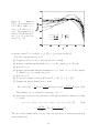
CAIN is a stand-alone FORTRAN Monte-Carlo code for the interaction involving high
energy electron, positron, and photons. Originally, it started with the name ABEL[1]
in 1984 for the beam-beam interaction in e+ e− linear colliders. At that time the main
concern was the beam deformation due to the Coulomb ﬁeld and the synchrotron radiation (beamstrahlung). Later, the pair creation by particle-particle collision was added,
and, it was renamed to CAIN when the interaction with laser beams (radiation by electrons/positrons and pair creation by photons in a strong laser ﬁeld) was added for the
γ-γ colliders.
CAIN home page is located at http://www-acc-theory.kek.jp/members/cain/
The ﬁrst version CAIN1.1[2], which is a combined program of modiﬁed ABEL and
a laser QED code, is limited because it cannot handle the laser interaction and the e+ e−
interaction simultaneously and does not accept mixed e+ e− beams. To overcome these
problems, CAIN2.0 was written from scratch. It now allows any mixture of e− , e+ , γ
and lasers, and multiple-stage interactions. The input data format has been refreshed
completely.
The physical objects which appear in the present version CAIN2.1e are two particle
beams, lasers, and external ﬁelds. Each of the two beams may consist of high-energy
electrons, positrons and photons. One of the beams may be absent. A basic assumption
is that each beam must be a ‘beam’, i.e., most particles in each beam go almost parallel.
(CAIN assumes the two beams go opposite direction. For the case they make a large
angle, you can apply CAIN command for Lorentz transformation so that the collision
looks head-on.) The lasers can go any direction. The present version accepts only constant
external ﬁelds.
The interactions that can be treated by the present version CAIN2.1e are
• Classical interaction (orbit deformation) due to the Coulomb ﬁeld.
• Luminosity between (e− e+ γ).
• Synchrotron radiation (beamstrahlung), and pair creation by high energy photons
(coherent pair creation) due to the beam ﬁeld.
• Interaction of high energy photon or electron/positron beams with laser ﬁeld, including the nonlinear eﬀect of the ﬁeld strength.
• Classical and quantum interactions with a constant external ﬁeld.
• Incoherent e+ e− pair creation by photons, electrons and positrons.
• In almost all interactions the polarization eﬀects can be included.
1.1
General Structure of Input Data
In this section we brieﬂy describe the structure of input data. CAIN is not intended for
interactive jobs because the computing time is normally more than several minutes. Every
3
intruction to the program is given in the input data. Two cases, a simple e+ e− collision
and a γ-γ collider, are given here as examples. For more detail look at the sections for
each command and the example input data ﬁles in the directory cain21e/in.
Consider a simple e+ e− collision. You have ﬁrst to deﬁne the two beams:
BEAM
RIGHT, KIND=2, NP=10000, AN=1E10, E0=500E9, SIGT=1E-4,
BETA=(1E-2,1E-4), EMIT=(3E-12,3E-14);
This deﬁnes the right-going electron (KIND=2) with the bunch population 1 × 1010 , energy
500GeV, bunch length 100µm, etc. Note that every command must end with a semicolon.
You can use variables and mathematical expressions (see Sec.2.5). For example, if you
prefer normalized emittance, you may write
SET
ee=500E9, gamma=ee/Emass, emitx=3D-6/gamma, emity=3D-8/gamma,
betax=1E-2, betay=1E-4,
sigx=Sqrt(emitx*betax), sigy=Sqrt(emity*betay);
BEAM RIGHT, KIND=2, NP=10000, AN=1E10, E0=ee, SIGT=1E-4,
BETA=(betax,betay), EMIT=(emitx,emity);
Emass is a reserved variable and Sqrt is a predeﬁned function. sigx and sigy are deﬁned
for later use. If you like millimeter instead of meter, you may say
SET
BEAM
mm=1E-3, sigz=0.1*mm;
........ SIGT=sigz, ......;
Now you know how to deﬁne the positron (KIND=3) beam. Obviously, BEAM LEFT,
KIND=3, . . .; will do.
For calculating the beam-beam force you need to tell CAIN about the mesh:
SET Smesh=sigz/2;
BBFIELD NX=32, NY=32, WX=8*sigx, R=sigx/sigy/2;
The deﬁnition of the longitudinal mesh Smesh may look bizzarre. This is because the
same mesh is used for luminosity calculation.
For computing the e+ e− luminosity, you have to say, for example,
LUMINOSITY KIND=(2,3), W=(0,2*ee,50), WX=8*sigx, WY=8*sigy, FREP=90*150;
if the rep rate is 90 bunches times 150Hz. WX and WY deﬁne the mesh region (See Sec.3.9).
Now you are ready to start the collision.
FLAG OFF ECHO;
PUSH Time=(-2.5*sigz,2.5*sigz,200);
ENDPUSH;
will track the beam over the speciﬁed time range in 200 steps. It is better to turn oﬀ the
echo before running. You can get the transient information (e.g., plot the beam proﬁle
during collision) by inserting commands (PLOT, WRITE etc) between PUSH and ENDPUSH.
If you want the bamstrahlung, you have to insert
4
CFQED
BEAMSTRAHLUNG;
before PUSH. After ENDPUSH you can plot (generate TopDrawer input ﬁle) the e+ e− differential luminosity by
PLOT LUMINOSITY, KIND=(2,3);
You can also plot particle distribution. For example, for plotting the photon (KIND=1)
energy spectrum,
PLOT
HIST, KIND=1, H=En/1E9, HSCALE=(0,ee/1E9,50),
TITLE=’Beamstrahlung Energy Spectrum;’,
HTITLE=’E0G1 (GeV); XGX
;’;
H deﬁnes the horizontal axis (energy in units of GeV).
You may want various outputs without repeating the time-consuming calculation. You
can do the following. After ENDPUSH, store all the variables and the particle data:
STORE FILE=’aaa’;
WRITE BEAM, FILE=’bbb’;
and restore in another input ﬁle
RESTORE FILE=’aaa’;
BEAM FILE=’bbb’;
PLOT ........;
γ-γ collider is more complex. Three steps, e-γ conversion of right-going electron,
that of left-going electron, and γ-γ collision, are needed. You can do these steps in one
job or in separate jobs using STORE/WRITE and RESTORE/BEAM FILE commands. The
attached example cain21e/in/NLCggCP.i executes the two conversions and NLCggIP.i
the collision at the interaction point.
For the conversion you deﬁne the lasers in addition to the initial electron beam:
LASER LEFT, WAVEL=laserwl, POWERD=powerd,
TXYS=(-dcp,0,off/2,-dcp),
E3=(0,-Sin(angle),-Cos(angle)), E1=(1,0,0),
RAYLEIGH=(rlx,rly), SIGT=sigt, STOKES=(0,1,0) ;
See Sec.3.4 for the meaning of the key words. The type of laser-electron and laser-γ
interactions has to be speciﬁed by LASERQED command:
LASERQED
LASERQED
COMPTON, NPH=5, XIMAX=1.1*xi, LAMBDAMAX=1.1*lambda ;
BREITW, NPH=5, XIMAX=1.1*xi, ETAMAX=1.1*eta ;
The PUSH-ENDPUSH loop is the same as in the e+ e− example.
After ENDPUSH write all the particle data by WRITE BEAM, FILE=... or, if you do not
want to include e-e collision, write the photon data selectively by WRITE BEAM, KIND=1, FILE=....
Then, read this ﬁle in the next job and simulate the γ-γ collision.
See Sec.2 for the basic grammer of the input data. See Sec.2.4 for a list of all the
available commands.
5
1.2
Change since the last version CAIN2.1b
There has been a version CAIN2.1d but the changes since then are only bug ﬁxes. Here
we list up the changes since CAIN2.1b.
• Unequal mesh of energy for diﬀerential luminosity has been introduced.
1.3
History until the last version CAIN2.1b
New entries on physics
• 2D diﬀerential luminosity dL/dE1 dE2 added.
• Lorentz transformation of lasers has been added.
• Field-strength dependence of the anomalous magnetic moment of electron is taken
into account in solving the Thomas-BMT equation.
• Polarization dependence of the beamstrahlung and the coherent pair creation has
been included.
• The kinematics in nonlinear QED subroutines was improved so as to accept nonrelativistic electrons/positrons.
• The ﬁnal polarization of electron in the nonlinear Compton scattering was added.
• Polarization change in linear and nonlinear QED, beamstrahlung and coherent pair
creation processes when event generation is rejected is now taken into account.
• Incoherent e+ e− pair creation by Breit-Wheeler, Bethe-Heitler, and Landau-Lifshitz
processes has been added.
• Luminosity with full polarization information (including linear polarization) can be
computed.
• Diﬀerential luminosities with unequal-space energy bins are introduced.
New entries on user interface
• Following pre-deﬁned variables have been added:
Kind, Gen
• Following pre-deﬁned functions have been added:
Min, Max,
AvrT, AvrX, AvrY, AvrS, SigT, SigX, SigY, SigS,
AvrEn, AvrPx, AvrPy, AvrPs, SigEn, SigPx, SigPy, SigPs,
TestT, TestX, TestY, TestS, TestEn, TestPx, TestPy, TestPs,
LumP, LumWP, LumWbin, LumWbinEdge,
LumEE, LumEEbin, LumEEbinEdge, LumEEH, LumEEP,
BesJ, DBesJ, BesK13, BesK23, BesKi13, BesKi53,
FuncBS, FuncCP, IntFCP
6
• Do-type sequence in PRINT/WRITE command became possible.
• Maximum number of characters of user parameters is increased to 16. Also, the
underscore ‘_’ is allowed in parameter names.
• The ﬂags for beamstrahlung and coherent pair creation, which had been deﬁned
in the BBFIELD command, were moved to a new command CFQED (constant-ﬁeld
QED). This is more logical becuase CAIN computes these phenomenon due to the
external ﬁelds, too.1 Acoording to this change, CFQED operand was added to CLEAR
command. Except for this change, input data ﬁles prepared for CAIN2.1b can be
used for CAIN2.1e.
• New commands STORE and RESTORE were added. You can store the variables and
the luminosity data for later jobs.
• Command PLOT FUNCTION was added.
Bugs (already ﬁxed in the present version)
• There was a bug in CLEAR BEAM command when applied during a PUSH ENDPUSH
loop. Fixed.
• A bug was found in the ﬁle source/physics/bb/bbmain/bbkick.f in solving the
equation of motion under the beam-beam force. It is a kind of double counting of
the beam-beam eﬀect. Fixed.
• Several bugs were found in DRIFT, EXTERNAL command. Fixed.
• There was a miss-spelled variable in subroutine EVUFN (in the directory
source/control/deciph). (This has been overlooked because of missing
IMPLICIT NONE.) Not very harmful. Fixed.
• Total helicity luminosity was not calculated, although diﬀerential helicity luminosity
was. (A bug in physics/lum/dlumcal.f) Fixed.
• PRINT/WRITE command did not correctly understand the KIND operand. Fixed.
• The polarization sign of the ﬁnal positron in the subroutine for linear Breit-Wheeler
process (source/physics/laser/nllsr/lnbwgn.f ) was wrong. Corrected.
• Linear polarization of ﬁnal photons in the linear Compton scattering was wrong.
(ξ1 , ξ3 ) used to come out as (−ξ3 , ξ1 ). Fixed.
2
Basic Grammer of the Input Data
2.1
System of Units
MKSA is used throughout. The particle energy and momentum are eV and eV/c, respectively. An exception is the luminosity which is expressed in cm−2sec−1 . The time (e.g.,
the laser pulse length, time coordinate of particles, etc.) is always expressed in units of
meter by multiplying the velocity of light.
1
Following this logic more faithfully, CAIN should have adopted the word SYNCHROTRONRADIATION
instead of BEAMSTRAHLUNG.
7
2.2
Characters
Upper and lower case alphabets are distinguished. The following characters have special
use:
= ; , ( [ { ) ] } ! < > ’
Also, the following characters are used in mathematical expressions:
+ - * / ^ = . ( [ { ) ] }
2.3
File Lines and Command Blocks
The input data is a collection of ﬁle lines. Upto 256 characters in a line are read in.
(This limitation can be easily changed by modifying the parameter statement in the main
program.)
If a character “!” is encountered, the whole text after it to the end of the ﬁle line is
considered as a comment, unless the “!” is in a pair of apostrophes. Apostrophe pairs
must close within a ﬁle line except for comment parts. Apart from the above two points,
the concept of ‘ﬁle line’ is irrelevant. Therefore, for example, continuing the two ﬁle lines
will give the same results, and the end of a command must explicitly said (by semicolon
“;”) without relying on the end-of-line.
The whole text, after comment part is eliminated, is divided into ‘command blocks’.
The end of a command block is indicated by a semicolon “;”. If “;” is inside a pair of
apostrophes, it is not considered to be a command terminator.
Each command block has the following structure:
operand, operand, · · · operand ;
command name
After the command name before the ﬁrst operand, there must be at least one blanck
character (unless there is no operand). Operands are separated by a comma “,” and the
number of blancks before and after “,” is arbitrary. (In some commands, “,” can be
replaced by one or more blancks). Unless stated in each command description in the next
section, the order of operands is arbitrary.
An operand is either a single keyword or of the form
keyword relational operator right hand side
A keyword is an alphanumerical string predeﬁned for each command. The relational
operator is either one of =, <, >, <=, >=, =<, =>, <>, ><. The right hand side is just a
number or an ‘expression’ (to be explained later) or of the form
( expression, expression, · · · expression)
The parenthesis ( ) may be replaced by [ ] or { }.
2.4
Commands
As stated above, each command block must start with a command name. The present
version has the following commands
FLAG
On-oﬀ ﬂags (echo, etc.). Sec.3.1.
SET
Deﬁne user variables. Sec.3.2.
BEAM
Deﬁne particle beams. Sec.3.3.
8
LASER
Deﬁne lasers. Sec.3.4.
EXTERNALFIELD Deﬁne external (static) electromagnetic ﬁeld. Sec.3.8.
LASERQED
Parameters for the laser-particle interaction. Sec.3.5.
CFQED
Parameters for the interaction between particles and constant electromagnetic ﬁeld (beamstrahlung and coherent pair creation). Sec.3.6.
BBFIELD
Method of calculation of the beam ﬁeld. Sec.3.7.
PPINT
Incoherent particle-particle interaction. Sec.3.10.
LUMINOSITY
Deﬁne what sort of luminosities to be calculated. Sec.3.9.
LORENTZ
Lorentz transformation. Sec.3.13.
DRIFT
Move particles in vaccuum or in external ﬁeld. Sec.3.12.
PUSH,ENDPUSH
Loop of time steps. Sec.3.11.
DO,ENDDO
Do loop. Sec.3.14.
IF,ELSE,ENDIF
If block. Sec.3.15.
WRITE,PRINT
Print on screen or on a ﬁle. Sec.3.16.
PLOT
Plot using TopDrawer. Sec.3.17.
CLEAR
Clear data or disable commands. Sec.3.18.
FILE
Open/close ﬁles. Sec.3.19.
HEADER
Deﬁne the header for graphic outputs. Sec.3.20.
STORE,RESTORE
Save/recall variables and luminosity values. Sec.3.21.
STOP
Stop run. Sec.3.22.
END
End of the input ﬁle. Sec.3.23.
The command names may be shortened if not ambiguous. Therefore, LASERQ is equivalent to LASERQED. This rule applies also to the operand keywords of all commands. (But
does not apply to parameter and function names.)
2.5
Expressions
In the example in Sec.1.1, the right hand sides of some operands are written in the form
of mathematical expressions. In general, ‘expression’ is a mathematical expression which
is almost identical to FORTRAN ﬂoating expression. It may contain
• Literal numbers, such as 2, 2.0, -3E-5, etc.
To indicate the exponent, any of E,e,D,d,Q,q may be used. Note that there is no
integer expression so that 2 is identical to 2.0.
• Operators +,-,*,/,^. Note that power is indicated by “^” instead of “**”.
• Parenthesis: ( [ { ) ] } . Must match.
• Pre-deﬁned parameters: There are three types of predeﬁned parameters. The ﬁrst
type is the universal constants that never change:
9
Pi
E
Euler
Deg
Cvel
Hbar
Hbarc
Emass
Echarge
Reclass
LambdaC
FinStrC
π
e = 2.718 . . .
Euler’s constant γE = 0.577 . . .
0.0174. . . = π/180. You can write, e.g., 10*Deg where the randian
unit is required.
Velocity of light (m/sec).
Planck’s constant (Joule·sec).
Planck’s constant times the velocity of light (eV·m).
Electron mass (eV/c2).
Elementary charge (Coulomb).
Classical electron radius (m).
Compton wavelength (m).
Fine structure constant.
The second type is the parameters whose values are determined by the program.
Users cannot change their values but can refer to.
T,X,Y,S
Running variables for particle coordinate (m).
En,Px,Py,Ps Running variables for energy-momentum (eV, eV/c). The energy
is En but not E.
Sx,Sy,Ss
Electron/positron spin. Helicity may be written approximately as
Ss*Sgn(Ps).
Xi1,Xi2,Xi3 Photon Stokes parameters ξ1 , ξ2 , ξ3 .
Kind
Particle species. 1,2,3 for photon, electron, positron.
Gen
Particle generation.
Time
Running variables for global time coordinate (m).
Ln,Lij
(n=0,1,2,3,4, i,j=0,1,2,3) Luminosity values used in PLOT LUMINOSITY
command.
W
Center-of-mass energy used in PLOT LUMINOSITY command.
The third type is those whose names are predeﬁned with default values and which
the user can change (by SET command) such as
MsgFile
Outfile
OutFile2
TDFile
MsgLevel
File reference number for echo, error messages, and default destination of PRINT command. (default=6)2
File reference number for voluminous outputs. The default destination of WRITE command. (default=12)
Other print output. Not used. (default=12)
TopDrawer ﬁle number. (default=8)
Message level. (default=0, i.e., error messages only)
2
The input ﬁle number is set to 5. If you want to change it, see the variable RDFL in the ﬁle
’cain21e/source/control/main/initlz.f’.
10
Rand
Debug
Smesh
Random number seed. Positive odd integer other than 1, default=12345.
You can reset random number at any time.
Debug parameter for the programmer. If you set Debug≥2, call and
return from major subroutines are announced. (default=0)
Longitudinal mesh size (m) for the calculation of beam-beam ﬁeld,
luminosity, etc. No default value.
• User-deﬁned parameters: Those deﬁned by SET command. Upto 16 characters consisting of upper/lower case alphabets, numericals, and underscore ‘_’. The ﬁrst
character must not be a numerical.
• Predeﬁned functions such as
Int,Nint,Sgn,Step,Abs,Frac,Sqrt,Exp,Log,Log10,
Cos,Sin,Tan, ArcSin,ArcCos,ArcTan,
Cosh,Sinh,Tanh, ArcSinh,ArcCosh,ArcTanh, Gamma,
Mod, Atan2, Min, Max
Deﬁntions are the same as in standard FORTRAN except Sgn and Step:
Sgn(x)=1, 0, −1, for x > 0, x = 0, x < 0.
Step(x)=1, 0, for x ≥ 0, x < 0.
Enclose the argument by ( ) or [ ] or { }. Separate arguments by “,” if there are
more than one argument (Mod, Atan2, Min, Max). (Number of arguments for Min
and Max is arbitrary.)
There are functions of other type, which are deﬁned for CAIN. See the next subsection Sec.2.6.
2.6
CAIN functions
In addition to the predeﬁned functions of general use, such as Sin and Cos, there are
other special functions intrinsic to CAIN. There is one limitation on the arguments of
the CAIN functions: the arguments must not contain any CAIN functions (due to the
problem of FORTRAN recursive call).
Beam statistics functions
Firstly, the number of particles, that of macro particles, the average coordinates/energymomentum and their r.m.s. values of the beam at the given moment are retrieved by
NParticle, NMacro,
AvrT, AvrX, AvrY, AvrS, SigT, SigX, SigY, SigS,
AvrEn, AvrPx, AvrPy, AvrPs, SigEn, SigPx, SigPy, SigPs,
BeamMatrix The calling sequence is common to these functions except BeamMatrix. Let
us take SigX as an example.
SigX(j,k) (j= 1 or 2 or 3, k= 1 or 2 or 3)
returns the horizontal r.m.s. size of right-going (j=1) or left-going (j=2) or both (j=3)
of the photon (k=1) or electron (k=2) or positron (k=3) beam. If there is one more
argument like
SigX(j,k,s0 )
11
then the particles are restricted to those in the region s0 − Smesh/2 ≤ s ≤ s0 + Smesh/2.
The variable Smesh must be deﬁned before.
BeamMatrix requires two more arguments
BeamMatrix(a,b,j,k,s0 ) (1≤a,b≤8)
The returned value is the average of xaxb where xa =(T,X,Y,S,En,Px,Py,Ps) for a=1 to 8.
(In units of m and eV or eV/c.)
Test particle variables
The coordinates and the energy momentum of the test particles can be retrieved by the
functions
TestT, TestX, TestY, TestS, TestEn, TestPx, TestPy, TestPs
The calling sequence is, for example, TestX(’name’) or TestX(n), where ’name’ is
the character string for the particle name and n is an expression representing an integer
−99 ≤ n ≤ 999. (See Sec.3.3 for the test particle name.)
Luminosity-related function
There are functions related to the luminosity:
Lum, LumH, LumP
LumW, LumWbin, LumWbinEdge, LumWH, LumWP
LumEE, LumEEbin, LumEEbinEdge, LumEEH, LumEEP
See Sec.3.9 for deﬁnitions for these functions.
Special functions
Bessel function Jn . (n must be an integer.)
BesJ(n,x)
Bessel function Jn (x). n must be an integer.
DBesJ(n,x)
Derivative of Bessel function, Jn (x).
Modiﬁed Bessel function Kν and its integral. In all the following functions, the last
argument k must be 1 or 2. When k = 2, the output is the function multiplied by ex.
The last argument may be omitted (equivalent to k = 1.)
BesK(ν,x,k)
Modiﬁed Bessel function Kν (x). (x > 0)
DBesK(ν,x,k)
Derivative of the modiﬁed Bessel function Kν (x). (x > 0)
BesK13(x,k)
Modiﬁed Bessel function K1/3 (x). (x > 0)
BesK23(x,k)
Modiﬁed Bessel function K2/3 (x). (x > 0)
BesKi13(x,k)
Integral of Modiﬁed Bessel function, Ki1/3 . (x > 0) See eq.(94) for the
deﬁnition of Ki.
BesKi53(x,k)
Integral of Modiﬁed Bessel function, Ki5/3 . (x > 0)
Functions for beamstrahlung and coherent pair creation.
12
FuncBS(x,Υ)
Beamstrahlung function F00 deﬁned in eq.(92). x (0 < x < 1) is the
photon energy in units of the initial electron energy. Υ > 0.
FuncCP(x,χ)
Spectrum function FCP of coherent pair creation deﬁned in eq.(108).
x (0 < x < 1) is the positron energy in units of the initial photon
energy. χ > 0.
IntFCP(χ,k)
Integral of FuncCP(x,χ) over 0 < x < 1. The√total rate of coherent
pair creation is given by multiplying by αm2 /( 3πEγ ). (See Sec.5.9).
k must be 1 or 2 (can be omitted if 1). If k = 2, the function is
multiplied by exp(8/3/χ).
3
Commands
A command, in general, has the following structure:
op1 , op2 , . . . , opn ;
command name
A command name is a string consisting of upper-case roman letters and numbers only.
There must be one or more than one blanck characters after a command name before the
ﬁrst operand.
‘opj ’ is an operand having either one of the following forms:
(a)
kwd
(b)
expr
(c)
kwd rel expr
(d)
expr rel expr
Here, ‘rel’ is a relational operator which is either one of =, <, >, <=, >=, =<, =>, <>,
><. ‘kwd’ is a keywaod, i.e., a string consisting of upper-case roman letters only, which is
predeﬁned for each command. ‘expr’ is a mathematical expression described in Sec.2.5.
An operand of the form (a) is a ﬂag-type operand. In some commands, the ﬁrst
operand must be a positional operand of the ﬂag-type. (For example, DO command must
be either DO WHILE or DO REPEAT.) In such a case, the “,” after the keyword may be
omitted. (There is no ambiguity because keywords do not contain blanck characters in
contrast to expressions.) FLAG command is special in that all the commas may be omitted
because all the operands are type(a).
The right-hand-side of type(c) can be (expr,expr,. . .), or can be a character string
for some operands
Now, let us describe the each command in detail. When describing the command
formats in this manual, the type-faced characters are those to be typed in the input data
as it is. (The variable names in the FORTRAN source also appear in type-face.) The
items embraced by square brackets [ ] may be omitted in some cases and the vertical
stroke “|” indicates an exclusive choice of one of the items. Thus, [A|B] means to choose
either one of A or B or to omit both. Note that [ ] and [ ] are diﬀerent.
The dagger † indicates that the operands to the left of it are positional operands.
The quantities printed in math-font in command syntax can be expressions.
13
3.1
FLAG
Set ﬂag. example:
FLAG ON ECHO OFF SPIN ;
The keywords ON and OFF act until the opposite one appears. ON is the default after FLAG.
Existing ﬂags
ECHO
input data echo (default=ON)
SPIN
include spin calculation (default=ON) (Sorry, spin calculation cannot be
avoided in the present version.)
3.2
SET
Deﬁnes parameters.
Syntax:
SET
3.3
[p = a ]
[, p = a ]
···
;
p
New or old parameter name. Upto 16 characters consisting of upper/lower
case alphabets, numericals, and underscore ‘_’. The ﬁrst character must
not be a numerical. Unchangeable predeﬁned parameters (Pi, Time, etc)
and the predeﬁned function names (Sin, etc) have to be avoided. All the
predeﬁned parameter names and function names start with an uppercase
letter. Therefore, a user parameter starting with a lower case alphabet will
never hit the predeﬁned ones.
a
An expression. See Sec.2.5.
BEAM
Deﬁnes a beam. (Append particles to the existing list.) There are two ways to create a
beam, one by specifying the Twiss parameters, etc, and the other by reading data from a
ﬁle.
Deﬁnition by Twiss parameters
Note that the beam is deﬁned on a plane s=constant, rather than on the t=constant
plane (snap shot). Thus, e.g., the bunch length is a spread in t rather than in s.
Syntax:
BEAM
RIGHT|LEFT, KIND=k, AN=N, NP=Np , E0=E0 ,
[TXYS=(t,x,y,s),] BETA=(βx,βy ), [ALPHA=(αx ,αy ),] [EMIT=(x,y ),]
[SIGT=σt,] [SIGE=σε ,] [GCUT=(nx ,ny ),] [GCUTT=nt ,] [GCUTE=nε ,]
[GAUSSWEIGHT=ig ,] [ELLIPTIC,] [TUNIFORM,] [EUNIFORM,]
[SLOPE=(θx ,θy ),] [CRAB=(ψx,ψy ),] [ETA=(ηx ,ηy ),]
[ETAPRIME=(ηx ,ηy ),] [ESLOPE=dε/dt,] [XYROLL=φxy ,]
[SPIN=(ζx ,ζy ,ζs ),] ;
14
RIGHT|LEFT Specify whether the beam is right-going or left-going.
k
Particle species. 1 for photon, 2 for electron, 3 for positron. If you cannot
remember these codes, you can do
SET photon=1, electron=2, positron=3 ;
BEAM RIGHT, KIND=electron . . .
N
Number of real particles.
Np
Number of macro-particles.
E0
Beam energy. (eV)
t,x,y,s
Location of the reference point and the time when the beam center comes
there. In units of meter. This is the point where the Twiss parameters
are to be deﬁned. Default=(0,0,0,0).
βx,βy
Beta functions (m).
αx ,αy
Alpha functions. Default=(0,0). The sign of α is positive when the beam
is going to diverge, whichever the beam is right-going or left-going.
x,y
R.m.s geometric emittance (rad·m). Deafault=(0,0).
σt
R.m.s. bunch length (m). Default=0.
σε
Relative r.m.s. energy spread. Default=0.
nx ,ny ,nt ,nε Gaussian tail cutoﬀ in units of corresponding sigmas. The default values
are 3.0 for nx and ny , and 2.5 for nt and nε . (For transverse variables the
cut oﬀ is done in the action variable, which means Ji /i ≤ n2i /2 (i=x,y).)
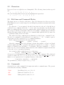
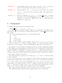
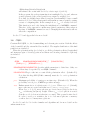
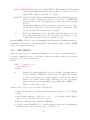
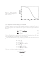
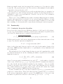
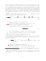
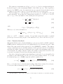
ig
0 or 1. There is a subtle problem on how to take into account the
Gaussian cut oﬀ (nx ,ny ,nt ) in the macro-particle weight. CAIN throws
away the random numbers outside this range and generates exactly Np
macro-particles. This means some fraction outside the region is moved
inside. Therefore, if the simple weight N/Np is assigned to macroparticles
(ig = 1), the eﬀective particle density would become slightly larger than
the physical value, although the sum of the weight is equal to N. If one is
interested in the quantities related to the density (such as luminosities),
this would cause an overestimation.
When ig = 0 (default), a correction factor is multiplied to the weight
such that the real particle density becomes correct. In this case, the sum
of the macro-particle weights is less than N. (When the default n’s are
adopted, for example, the correction of the weight amounts to ∼3.4%.)
In most cases, ig = 0 will be better.
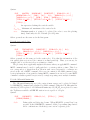
ELLIPTIC
Uniform transverse distribution. (Default is Gaussian.) (x, y) distribution is a uniform ellips with radii (2σx , 2σy ), where σj = j βj (j=x,y).
In this case the beam is parallel, in spite the ﬁnite emittances are speciﬁed. The emittance and beta are only used to deﬁne σx,y . ALPHA and
GCUT are not used.
15
Figure 1: Physical charge
density (dashed curve)
and the simulated density
(solid) for ig =0 and 1
TUNIFORM
√
Uniform t-distribution. (Default is Gaussian.) The full length is 2 3σt.
GCUTT is not used.
EUNIFORM
Uniform E-distribution.
(Default is Gaussian.) The full relative energy
√
spread is 2 3σε . GCUTE is not used.
θx,θy
Angle oﬀset (radian). The right and left-going beams have the same sign
of slope when there is a crossing angle. Default=(0,0).
ψx,ψy
Crab angle ∂x(y)/∂t. (radian). Positive when the bunch tail has larger
x (y).
When the full crossing angle in the horizontal plane is φcross and this is
to be compensated by the crab angle, the SLOPE and CRAB parameters
should be SLOPE=φcross /2, CRAB=φcross /2, for both right-going and leftgoing beams.
If you are not conﬁdent, after beam deﬁnition try, for example,
DRIFT T=t0-dt ;
PLOT SCAT, H=S, V=X,
HSCALE=(smin,smax), VSCALE=(xmin,xmax),
HTITLE=’S(m)’, VTITLE=’X(m)’ ;
DRIFT T=t0 ;
PLOT SCAT, NONEWPAGE, H=S, V=X,
HSCALE=(smin,smax), VSCALE=(xmin,xmax),
DRIFT T=t0+dt ;
PLOT SCAT, NONEWPAGE, H=S, V=X,
HSCALE=(smin,smax), VSCALE=(xmin,xmax),
with appropriate deﬁnitions of t0, smin etc. The DRIFT command transports the beam to the plane t=constant (snap shot). NONEWPAGE operand
suppresses page break so that the (s,x) proﬁles at diﬀerent times appear
on the same page.
ηx , ηy
Eta function (m).
ηx , ηy
Derivative of eta function.
dε/dt
Coherent energy slope from bunch head to tail (1/m).
φxy
Roll angle of the beam in the x-y plane. (radian)
ζx ,ζy ,ζs
Polarization vector. Default=(0,0,0). Note the sign of ζs for left-going
particles. In the case of photon beams, these are the Stokes parameter
(ξ1 , ξ2 , ξ3 ). The basis vector of the Stokes parameter is (e(1) , e(2) , e(3) )
16
where e(3) is the unit vector along the particle momentum, e(1) is the
unit vector along ex − e(3) (e(3) ·ex ), and e(2) = e(3) ×e(1) .
See Sec.5.3 for rigorous deﬁnitions.
Read particle data from a ﬁle
Syntax:
FILE=fn |’ﬁle name’,
BEAM
[N=Np ,]
[NAMELIST,] ;
fn
File reference number.
ﬁle name
Existing ﬁle name. Must be enclosed by apostrophes. Either full path or
relative path. Note that CAIN is run in the directory cain/exec.
The ﬁle is opened with the reference number 99 and is closed immediately
after reading.
Np
Maximum number of macro-particles to be read in from ﬁle. If 0, nonactive. Default=0.
NAMELIST
FORTRAN NAMELIST format. Othewise the standard format.
Reading ﬁle stops when one of the following conditions are satisﬁed.
• Np Reached (when Np > 0).
• A ﬁle line found whose ﬁrst three characters are ‘END’ in the case of the
standard format. Or, END=.TRUE. found in the case of the NAMELIST
format.
• End of ﬁle detected.
In the case of the standard format, the ﬁle is assumed to be created by the following
FORTRAN statement.
WRITE(*,’(I2,I6,1X,A4,1P12D20.12)’) KIND,GEN,NAME,WGT,
1
(TXYS(I),I=0,3),(EP(I),I=0,3),(SPIN(I),I=1,3)
Here, NAME is blanck unless the particle is a test particle or a lost particle or an incoherentpair particle, WGT is the number of real particles expressed by one macro-particle and GEN
is an integer expressing the generation (1 for the initial particles, 2 for secondaries, etc.).
SPIN is the polarization vector for electron/positron and the Stokes parameter for photons.
The ﬁle can also be MATHEMATICA style (automatically detected). The format
string is (’{’,I1,’,’,I5,’,’,A4,12(’,’,1PD19.12),’},’)
In the case of the NAMELIST format, the namelist BEAMIN must be inserted for each
particle.
&BEAMIN
KIND=2, GEN=1, PNAME=’
’, WGT=0.0, TXYS=0.0, 0.0, 0.0, 0.0,
EP=0.0, 0.0, 0.0, 1.0, SPIN=0.0, 0.0, 0.0,
END=.FALSE., SKIP=.FALSE.
&END
17
Here, the r.h.s. show the number of data, the data type, and the default. The last
component of EP, i.e., Ps , must not be zero. All the particles
√ must be either right- or
left-going. (Actually the particle energy is calculated from p2 + m2. The input data is
not used.)
If the ﬁrst character of PNAME is T, the particle is treated as a test particle. (The test
particle name must be unique.) PNAME should be blanck for normal particles.
If SKIP=.TRUE., the present data is omitted. If END=.TRUE., the present data and all
the following data are ignored. Comments in NAMELIST statements follow the local rule
on the platform.
To modify the ﬁle data (shift of origin, rotation, etc) can be done to some extent by
using the command LORENTZ.
Test particles
Deﬁnition of test particles can also be done by BEAM command. One BEAM command is
needed for each test particle. The number of test particles times the number of PUSH time
steps must be less than 5000 (parameter MTSTP in the ﬁle ’cain/source/include/tstpcm.h’).
Test particles do not create a ﬁeld but feel a ﬁeld. They do not interact with lasers and
do not create particles (such as beamstrahlung, incoherent pair, etc). Therefore, ‘test
photon’ does not make sense.
Coordinates and energy-momentum of test particles can be refered to at any time by
functions TestT, etc. See Sec.2.6.
Syntax:
BEAM
TESTPARTICLE,
P=(px ,py ,ps ) ;
NAME=n,|’name’,
KIND=k,
[TXYS=(t,x,y,s),]
n,name
A test particle must have a name, consisting of upto 3 characters. The
‘name’ (left-adjusted) must be enclosed by a pair of apostrophes. It can
also be speciﬁed by an integer −99 ≤ n ≤ 999, which is converted to a
decimal character string (right-adjusted). Thus, NAME=1 and NAME=’ 1’
is identical. (In the computer, one character ‘T’ is added at the top. Thus,
NAME=999 becomes T999.)
k
Particle specie.
t,x,y,s
Location of the test particle (m).
px , py , ps
3-momentum (eV/c). ps must not be zero (i.e., either right-going or
left-going).
What is actually deﬁned by the particle variables (t, x, y, s) and (E, px , py , ps ) is not
a particle at a deﬁnite space-time coordinate, but rather is a straight trajectory (a world
line) which passes the space-time point (t, x, y, s). At the time when the PUSH command
is executed, they are ﬁrst pulled to the intercept on t = t0 plane, where t0 is the starting
time of the PUSH loop.
When a BEAM command is inserted within a PUSH loop, the particles are taken to the
corresponding time t=Time. However, it is safer not to insert BEAM command within PUSH
18
loop unless you know well what is going on. One exception is the test particles, which in
some cases you want to create during a PUSH loop (for example to see the behavior of a low
energy particle created during interaction). If you do not want them to be time-shifted in
such cases, you can deﬁne the TXYS operand as TXYS=(Time,. . .), where Time is the PUSH
running time (‘present time’).
3.4
LASER
Deﬁnes a laser. There can be upto 5 lasers but this can easily be increased (parameter
MLSR in source/include/lasrcm.h). One LASER command deﬁnes one laser. Note that
lasers, if there are more than one, act incoherently. Their interference eﬀects cannot be
included in the present version.
The longitudinal (time) pulse shape can be Gaussian or trapezoidal but the transverse
is Gaussian only.
Syntax:
LASER
[RIGHT|LEFT,] WAVELENGTH=λL , POWERDENSITY=Ppeak ,
(3)
(3)
(1)
(1)
E1=(e(1)
[TXYS=(t,x,y,s),] E3=(e(3)
x ,ey ,es ),
x ,ey ,es ),
RAYLEIGH=(β1,β2), [GCUT=ncut ,] SIGT=στ |TTOT=τtot, [GCUTT=ntcut ,]
[TEDGE=τedge ,] [STOKES=(ξ1 ,ξ2 ,ξ3 ),] ;
RIGHT|LEFT Right-going or left-going. If RIGHT(LEFT) is speciﬁed, the laser acts only
onto the left(right)-going particles (to save computing time). If omitted,
acts on both.
λL
Laser wavelength (m).
Ppeak
Peak power density (Watt/m2 ).
t,x,y,s
Laser focal point and the time when the laser pulse comes there (m).
(3) (3)
(3)
along the direction of laser propagation.
(e(3)
x , ey , es ) Unit vector e
(1) (1)
(1)
(e(1)
perpendicular to e(3) . (e(1) , e(2) , e(3) ) with e(2) =
x , ey , es ) Unit vector e
e(3) ×e(1) forms a right-handed orthonormal frame. e(3) and e(1) need not
be normalized exactly and need not be perpendicular to each other exactly (The component parallel to e(3) is subtracted from e(1) by Schmidt
orthogonalization).
β1,β2
Rayleigh length in e(1) , e(2) direction. (meter)
ncut
Cut oﬀ of transverse tail in units of sigmas. Default=2.5.
στ
R.m.s. pulse length (times velocity of light) in power, not in ﬁeld amplitude, assuming Gaussian structure. (meter)
ntcut
Cut oﬀ of longitudinal tail in units of sigmas for Gaussian time structure.
Default=2.5.
τtot
Total pulse length for trapezoidal longitudinal structure (meter). Either
one of SIGT or TTOT must be speciﬁed.
19
τedge
Longitudinal edge length (meter) for trapezoidal time structure. The
ﬂat-top length is then τtot − 2τedge . Default=0 (i.e., rectangular shape).
ξ1 ,ξ2,ξ3
Stokes parameter deﬁned in the (e(1) , e(2) , e(3) ) frame. Default=(0,0,0).
See Sec.5.7.1 for more detail.
3.5
LASERQED
Deﬁnes the method and parameters for the calculation of the interaction between lasers
and particles.
Syntax:
LASERQED
COMPTON|BREITWHEELER[,]† NPH=nph , [NY=ny ,]
[NLAMBDA=nλ ,] [NQ=nq ,] XIMAX=ξmax , LAMBDAMAX=λmax ,
ETAMAX=ηmax , [PMAX=pmax ,] [ENHANCEFUNCTION=fenh ,] ;
[NXI=nξ ,]
COMPTON|BREITWHEELER Speciﬁes which parameters to deﬁne here.
nph
Maximum number of laser photons to be absorbed in one process.
If < 0, turn oﬀ Compton or Breit-Wheeler.
If =0, use linear Compton/Breit-Wheeler formula.
If ≥ 1, use nonlinear formula.
Note that nph = 0 and nph = 1 are diﬀerent. The former is the limit of ξ → 0,
which contains nph = 1 term only, whereas the latter is a truncation of the
exact series with respect to nph . When nph = 0, none of the variables (ny , nξ ,
nλ , nq , ξmax , λmax , ηmax ) are needed.
When nph ≥ 1, only longitudinal polarization is considered and the lasers must
be circularly polarized by 100% (i.e., ξ1 = ξ3 = 0, ξ2 = ±1).
ny
Number of abscissa for ﬁnal energy. Default=20.
nξ
Number of abscissa for ξ parameter. Default=20.
nλ
Number of abscissa for λ parameter. Applies to Compton case only. Default=20.
nq
Number of abscissa for q parameter. Applies tp Breit-Wheeler case only. Default=50.
ξmax
Maximum value of ξ for the table.
λmax Maximum value of λ for the table. Applies to Compton case only.
ηmax Maximum value of η for the table. Applies to Breit-Wheeler case only.
pmax Maximum probability of events per one time step. If the computed probability
exceeds pmax , CAIN of present version stops with a message.
fenh
Deﬁnes a function in order to enhance a part of spectrum. It is deﬁned as an
expression containing Y as the ﬁnal energy parameter (0 ≤Y≤ 1). Its value
must be ≥ 1 for 0 ≤Y≤ 1. Generally speaking, Y close to 1 generates low
energy charged particles. For example,
20
ENH=1+Step(Y-0.8)*(Y-0.8)*10
will enhance the events with Y> 0.8 by a factor upto 3 (at Y=1).
In the program, the real spectrum function is multiplied by fenh and, when an
event is generated, the created particles are asigned a weight 1/fenh .
Note that fenh slightly larger than 1 is useless (even harmful) because a small
fraction 1−1/fenh of the parent particle will remain as a macro-particle, causing
a waste of computing time. In the example above, fenh = 1 exactly for Y<0.8.
This function is used only during the initialization by LASERQED command.
Therefore, if the expression contains user-deﬁned parameters, their values at
the time of LASERQED command are used. Changing them afterwards will not
aﬀect the computation.
See Sec.5.7.3 and Appendix.A for more detail
3.6
CFQED
Constant-Field QED, i.e., the beamstrahlung and coherent pair creation. Both the eﬀects
of the beam ﬁeld and the external ﬁeld are included. The angular distribution of the ﬁnal
particles is not included.
When the polarization ﬂag (see below) is on, all the polarization eﬀects (longitudinal
and transverse spin of electron/positron and linear and circular polarization of photon)
are included.
Syntax:
CFQED
BEAMSTRAHLUNG|PAIRCREATION[,]†
[PMAX=pmax ,] [WENHANCE=wenh ,] ;
[POLARIZATION,]
BEAMSTRAHLUNG|PAIRCREATION Speciﬁes which parameters to deﬁne here. Only one
of these may be speciﬁed by one CFQED command.
POLARIZATION Flag to take into account all the polarization eﬀect. (default=No).
Note that the ﬂag SPIN (FLAG command) must also be on for polarization
calculation.
pmax Maximum probability of events per one time step. (Default=0.1). When the
probability exceeds pmax , CAIN stops with a message.
wenh Enhancement factor of radiation rate. 0 ≤ wenh . When wenh = 1 (default),
macro-photons are created such that nmacroγ /nmacroe = nrealγ /nreale
When wenh > 1 (< 1), macro-photons are created more (less) by the factor
wenh , each having less (more) weight. When wenh = 0, no photon is created
(but the recoil of electron is taken into account.) This operand is introduced
in order to avoid poor statistics due to too less macro-photons or memory
overﬂow due to too many macro-photons.
See Sec.5.8 and Sec.5.9 for the formulas and algorithm and for more detail on the
enhancement factor.
21
3.7
BBFIELD
Deﬁne the parameters for the calculation of beam-beam ﬁeld.
Syntax:
BBFIELD
WX=wx1 |WX=(wx1 [,wx2 ]), [WXMAX=wxm1 |WXMAX=(wxm1 ,wxm2),]
R=r, [NX=nx ,] [NY=ny ,] [PSIZE=∆,] [NMOM=nmom ,] ;
wx1 ,wx2
Horizontal width of the mesh in meters for right and left-going beams.
If wx2 is not speciﬁed, wx2 = wx1 is adopted. No default for wx1 .
wxm1,wxm2 If WXMAX is given, the with of the mesh region can vary in the range
(wx , wxm ) when the beam fraction outside the range deﬁned by WX and R
is signiﬁcant. Note wxm ≥ wx.
r
Aspect ratio (wx /nx )/(wy /ny ) of the horizontal to vertical mesh size.
This is common to right and left-going beams. No default.
nx ,ny
Number of horizontal and vertical bins. Present version uses Fast Fourier
Transformation so that a power of 2 is the best choice. Other numbers are
also allowed but those of the form 2n or 3×2n or 5×2n are recommended.
Default=32.
∆
Macro-particle size in units of the bin size. Macro-particles are treated as
a rectangular of uniform distribution. Must be 0 ≤ ∆ ≤ 1. Default=1.
nmom
For (x, y) points outside the mesh region, a harmonic expansion using the
elliptic coordinate is used. The parameter nmom speciﬁes the truncation
of harmonics. nmom = 0 takes only the total charge term and nmom < 0
ignores the ﬁeld outside. Default=10.
Note that the particles outside mesh region receive the beam-beam kick
unless nmom < 0, but the ﬁeld created by them is not taken into account.
See Sec.5.6 for more detail.
Note that the longitudinal mesh size, which is common to beam-beam ﬁeld and luminosity
calculations, has to be deﬁned by the parameter Smesh by the SET command. Its value
at the time when PUSH started is used thoughout the PUSH loop.
3.8
EXTERNALFIELD
Deﬁne external ﬁeld. The present version allows only a constant ﬁeld over an interval
bordered by two parallel planes.
Syntax:
EXTERNALFIELD
[S=(s1,s2 ),]
[B=(Bx ,By ,Bs ),] ;
[V=(cx ,cy ,cs ),]
[E=(Ex ,Ey ,Es ),]
sj , cj
Deﬁne the range of the ﬁeld as s1 ≤ cx x + cy y + cs s ≤ s2 .
Must be s1 < s2 . Default s1 = −∞, s2 = +∞ and (cx ,cy ,cs )=(0,0,1).
Ej
Electric ﬁeld components in units of V/m. Default=(0,0,0).
22
Bj
3.9
Magnetic ﬁeld components in units of Tesla. Default=(0,0,0).
LUMINOSITY
Deﬁne the transverse mesh size, number of bins, etc, for luminosity calculation. One
luminosity command is needed for each combination of particles γ, e− , e+ , right-going
and left-going. Thus, there can be at most 9 LUMINOSITY commands.
Syntax:
LUMINOSITY
KIND=(kr ,kl ), [FREP=frep ,]
[W=(Wmin ,Wmax ,nbin ),|W=(W0 ,W1 ,. . .,Wnbin ),]
[E1=(E1min ,E1max [,n1bin ]),|E1=(E1,0 ,E1,1 ,. . .,E1,n1bin ),]
[E2=(E2min ,E2max [,n2bin ]),|E2=(E2,0 ,E2,1 ,. . .,E2,n2bin ),] WX=(wx [,wxm ]),
WY=(wy [,wym ]), [HELICITY,] [ALLPOL,] ;
kr ,kl
Particle species of right and left-going beams.
frep
Repetition frequency (Hz). Used for the luminosity scale only. Default=1Hz.
Wmin,Wmax ,nbin Parameters for diﬀerential luminosity with respect to the center-ofmass energy W . (Wmin ,Wmax) is the range in eV and nbin is the number
of bins. If (Wmin ,Wmax) is not given, the center-of-mass spectrum is not
calculated. Default for nbin is 50.
Wj ,nbin
Deﬁne the center-of-mass energy bins in the case of non-equal spaced
bins. nbin is the number of bins, W0 is the lower edge of the ﬁrst bin
and Wnbin is the upper edge of the last bin. nbin must be ≥ 3 in order to
distinguish from the equal-space case.
E1min ,E1max ,n1bin ,E2min ,E2max ,n2bin 2-D diﬀerential luminosity dL/dE1 dE2 . (Ejmin ,
Ejmax ) is the range in eV and njbin is the number of bins. (j=1 for rightgoing beam and j=2 for left-going beam.) Both or none of E1 and E2
have to be speciﬁed. If none is speciﬁed, 2-D luminosity is not calculated.
Default for ni, bin is 50.
Ei,j ,ni,bin (i = 1, 2) Deﬁne non-equal spaced bins. Similar to the case of the centerof-mass energy.
wx ,wy
Full horizontal/vertical width of the mesh region (m). The origin is
adjusted automatically from time to time.
wxm ,wym
Maximum width of the mesh region (m). If not given, wx (wy ) is used
throughout. If given, an increased size upto wxm (wym ) is used when
a signiﬁcant particle fraction gets out of the mesh region deﬁned by
(wx , wy ). The number of mesh points is determined automatically.
HELICITY
Calculate luminosity for every combination of helicity, (++), (−+), (+−),
(−−).
ALLPOL
Calculate luminosity for all possible 16 combinations of the spins. (see
Sec.5.5.2 for detail.)
23
All the LUMINOSITY commands must have the same value of wx ,wy ,wxm,wym , and frep .
(Specify them at the ﬁrst LUMINOSITY command.)
Note that the longitudinal mesh size, which is common to beam-beam ﬁeld and luminosity calculations, has to be deﬁned by the parameter Smesh by the SET command.
The luminosity is actually computed by the PUSH-ENDPUSH loop. The calculated luminosity can be referred to by the following functions. (If during the loop, the accumulated
luminosity upto that moment is returned.)
Lum(kr ,kl )
Luminosity of KIND=(kr ,kl ) in units of cm−2 sec−1 .
LumH(kr ,kl ,h)
Helicity luminosity: helicity combination (++) (h = 1), (−+) (h =
2), (+−) (h = 3), (−−) (h = 4). h = 0 will give the total luminosity
Lum(kr ,kl ). (cm−2 sec−1)
LumP(kr ,kl ,s1 ,s2 ) Polarization luminosity. (0 ≤ s1 ≤ 3, 0 ≤ s2 ≤ 3) See Sec.5.5.2
for deﬁnition. (cm−2sec−1 )
LumW(kr ,kl ,n)
Diﬀerential luminosity in the n-th bin. (cm−2sec−1 /bin)
LumWbin(kr ,kl ,n) Bin center (eV) of the n-th bin. If n = 0, the number of bins is
returned. (Error if n < 0 or n is larger than the number of bins.)
LumWbinEdge(kr ,kl ,n) Bin edge (eV) of the n-th bin. (0 ≤ n ≤ number of bins.
n = 0 is the lower edge of the ﬁrst bin and n =number of bis is the
upper edge of the highest bin. (Error if n < 0 or n is larger than
the number of bins.)
LumWH(kr ,kl ,n,h) Diﬀerential helicity luminosity. (cm−2sec−1 /bin)
LumWP(kr ,kl ,n,s1 ,s2) Diﬀerential polarization luminosity. (0 ≤ s1 ≤ 3, 0 ≤ s2 ≤ 3)
See Sec.5.5.2 for deﬁnition. (cm−2sec−1 /bin)
LumEE(kr ,kl ,n1,n2 ) 2-D diﬀerential luminosity dL/dE1 dE2 for the bin (n1 ,n2).
(cm−2 sec−1 /bin)
LumEEbin(kr ,kl ,l,n) Bin center (eV) of the n-th bin of E1 (l=1) or E2 (l=2). If
n = 0, the number of bins is returned. (Error if n < 0 or n is larger
than the number of bins.)
LumEEbinEdge(kr ,kl ,l,n) Bin edge of the n-th bin of E1 (l=1) or E2 (l=2). See
LumWbinEdge for the deﬁnition of n.
LumEEH(kr ,kl ,n1 ,n2,h) 2-D diﬀerential helicity luminosity
LumEEP(kr ,kl ,n1 ,n2,s1 ,s2 ) 2-D diﬀerential polarization luminosity.
These functions can be included in expressions. Thus, you can write the computed luminosity on a ﬁle. In particular, the only way to retrieve the 2-D luminosity dL/dE1 dE2
is to use the above functions because PLOT LUMINOSITY command cannot plot it (KEK
TopDrawer cannot draw 3-D plot). So, for example, to write e+ e− luminosity, say
SET m1=LumEEbin(2,3,1,0), m2=LumEEbin(2,3,2,0);
WRITE ((LumEE(2,3,n1,n2),n1=1,m1),n2=1,m2),
FORMAT=(. . .);
If you are satisﬁed with a pre-deﬁned format, you can use PRINT/WRITE LUMINOSITY
command.
24
3.10
PPINT
Incoherent particle-particle interaction such as incoherent pair creation and bremsstrahlung.
The following processes are included:
Breit-Wheeler
γ + γ → e− + e+
Bethe-Heitler
γ + e± → e± + e− + e+
Landau-Lifshitz
e + e → e + e + e− + e+
Bremsstrahlung
e+e→ e+e+γ
All the processes except for Breit-Wheeler are cvalculated using the virtual photon
approximation.
The circular polarization eﬀect of the initial photons is included in the Breit-Wheeler
process but all other polarization eﬀects are ignored.
Particles created by incoherent processes do not contribute in creating the beam ﬁeld.
Also note that the parent macro-particles do not change by particle-particle interaction.
All these come from the actual situation in linear colliders where the incoherent particles
are much less in number compared with the initial particles.
Syntax: Specify virtual photon options
PPINT
LOCAL
VIRTUALPHOTON[,]†
[LOCAL,] [FIELDSUPPRESSION,] [EMIN=Emin ,] ;
Flag to adopt local virtual photon, i.e., to ignore the eﬀects due to the
ﬁnite transverse extent of virtual photons. Default is non-local.
FIELDSUPPRESSION Flag to include the virtual-photon suppression eﬀect due to strong
external ﬁelds (normally, the beam-ﬁeld by the on-coming beam). This
can be eﬀective when LOCAL is not speciﬁed. See section 3.4 of [6]. Default: does not include this eﬀect.
Emin
Minimum energy of ﬁnal electron/positron energies in eV. Default is twice
the rest mass of electron. = 1.022. . .E6. This parameter is not directly
related to virtual photons but included here because it is common to all
the processes. The purpose of this parameter is to save computing time.
The creation of pairs does not take too much computing time but to track
extremely low-energy pairs in a strong beam ﬁeld is very expensive. The
worst ones are the pair particles having the sign of charge opposite to
that of the on-coming beam because they are trapped in the strong ﬁeld
region. If you are not interested in them, you can eliminate them during
the PUSH loop as
CLEAR BEAM, INCP, RIGHT, KIND=2;
CLEAR BEAM, INCP, LEFT, KIND=3;
if the right(left)-going beam is electron(positron).
Syntax: Specify individual processes
PPINT
BW|BH|LL|BREMSSTRAHLUNG[,]†
[ENHANCE=fenh ,] ;
25
[RIGHT,]
[LEFT,]
BW,BH,LL,BREMSSTRAHLUNG Specify one of Breit-Wheeer, Bethe-Heitler, Landau-Lifshitz,
and Bremsstrahlung interactions. If more than one of these are needed,
apply PPINT command repeatedly. No default.
RIGHT,LEFT Applies to Bethe-Heitler and Bremsstrahlung. The Bethe-Heitler process
has two possible combinations, namely, (γ,e± ) and (e± ,γ). RIGHT/LEFT
option speciﬁes the photon is right-going or left-going or both. Default
is both.
The Bremsstrahlung is treated as the interaction between real e± and a
virtual photon. Therefore, it also has two possible combinations. This
operand speciﬁes which beam is the real particle.
fenh
Event rate enhancement factor. It is unity when the number of created
macro-pairs is the same as the expected number of real pairs, i.e., the
weight of the pair particle is 1/fenh . Default fenh =0.1.
In using ABEL one had to deﬁne the minimum scattering angle and minimum transverse
momentum. This was due to the ultra-relativistic approximation employed there. CAIN
does not need these parameters.
3.11
PUSH, ENDPUSH
Deﬁne the time step loop of tracking. Tracking is done by a pair of commands instead of
one single command in order to allow users to take action such as print, plot, insert test
particles, etc, at arbitrary time steps.
Syntax:
PUSH
Time=(t0 ,tf ,nt ) ;
. . . any commands . . .
ENDPUSH
;
t0,tf
Start and end time (multiplied by velocity of light) of tracking (meter).
Note the spelling of Time which contains lower case alphabet in contrast
to other operand keywords consisting of upper case letters only. In fact,
Time is a pre-deﬁned variable name. Therefore, you can, for example,
print its current value during PUSH loop by PRINT Time, FORMAT=. . ..
nt
Number of time steps. (≥ 0)
Actual control of the loop is done in the following way.
• Before the ﬁrst time step, all the particles are made to drift to t = t0 (by straight
lines).
• At the PUSH command of j-th loop (j = 0, 1, . . . , nt ), the time variable Time is
set to tj = t0 + j∆t where ∆t = (tf − t0 )/nt .
• Execute commands between PUSH and ENDPUSH.
• Control comes to ENDPUSH. If j < nt , make tracking (beam-beam, beamstrahlung,
laser interaction etc) for the time step tj ≤ Time ≤ tj+1 .
26
• If j < nt, returns to PUSH.
Note that the commands between PUSH and ENDPUSH are executed nt + 1 times. If nt = 0,
the actions taken are to drift all particles to t0 and to do commands between PUSH and
ENDPUSH once. If nt < 0, CAIN stops at PUSH with an error message rather than at
ENDPUSH.
3.12
DRIFT
Drift the particles to a certain time or to a certain s coordinate.
Syntax:
DRIFT
T=t1 |DT=∆t|S=s1,
[EXTERNALFIELD,] ;
[RIGHT,]
[LEFT,]
[KIND=k|(k1 ,k2 ),]
t1
Drift until Time=t1 (meter).
∆t
Drift over time interval ∆t (meter).
s1
Drift to s coordinate = s1 (meter).
In any of the three cases T, DT, and S, the particles may go backwards in
time depending on the parameters.
RIGHT,LEFT Drift right- or left-going particles only.
k
Drift only particles of kind k.
EXTERNALFILED Take into account the external ﬁeld.
When there is only external ﬁeld without beam interaction, DRIFT EXTERNAL is much
better (more accurate and faster) than the PUSH command. The diﬀerence is that DRIFT
EXTERNAL uses an exact solution in a constant ﬁeld whereas PUSH carries out step-by-step
integration, and that PUSH accepts only t as the independent variable while DRIFT also
allows s (as in most accelerator program codes).
How to use DRIFT EXTERNAL may be understood by the following example. Suppose
that the region s1 < s < s2 is shined by a laser. An electron beam comes from the left
and goes through the laser region to created back-scattered photons, and subsequently
goes through a magnetic ﬁeld region s3 < s < s4 . If the interval (s2, s3 ) is shorter than
the bunch length, the bunch head is already in the ﬁeld region when the tail gets out of
the laser region. If you use PUSH command, you have to track the beam till the end of
the magnetic ﬁeld region. Instead, you can do more elegantly,
Deﬁne electron beam
BEAM .....
Deﬁne laser
LASER .....
Deﬁne laser QED parameters
LASERQED .....
Start push without magnetic ﬁeld
PUSH ....
End push
ENDPUSH;
Deﬁne external ﬁeld
EXTERNALFIELD ....
Pull back the beam to the plane s3
DRIFT S=s3;
DRIFT S=s4, EXTERNALFIELD; Calculate the ﬁeld eﬀects
27
3.13
LORENTZ
Coordinate transformation (shift of origin, rotation, Lorentz transformation) of particle
coordinate, energy-momentum, polarization, etc. Using this command, you can transform a collision at an angle into a head-on collision.
Syntax:
LORENTZ
[TXYS=(∆t,∆x,∆y,∆s),] [ANGLE=φ,] [BETAGAMMA=βγ ,]
[AXIS=(ax ,ay ,as ),] [EV=(evx ,evy ,evs ),] [NOBEAM,] [RIGHT,] [LEFT,]
[KIND=k|(k1 ,k2 ),] [EXTERNALFIELD,] [LASER,] ;
(∆t, ∆x, ∆y, ∆s) Shift of origin. (m)
φ
Spacial rotation angle (radian). (rotation of the coordinate axis.)
βγ
Lorentz boost parameter β × γ. (Boost of the coordinate axis).
(ax, ay , as ) Unit vector along the rotation axis. Need not be normalized exactly.
(evx , evy , evs ) Unit vector along the boost direction. Need not be normalized exactly.
NOBEAM
No transformation of particles. If speciﬁed, RIGHT, LEFT, KIND operands
are ignored.
RIGHT,LEFT Select right- or left-going particles only. If omitted, both are transformed.
k
Select only particles of kind k. If omitted, all species are transformed.
EXTERNALFIELD Lorentz transformation of external ﬁeld (transformation of the ﬁeld
strength and the boundary).
LASER
Lorentz transformation of lasers.
The three types of transformations are carried out in the order of the input keywords TXYS,
ANGLE, BETAGAMMA. With one LORENTZ command, each transformation can be speciﬁed at
most once.
Note that, for any type, the transformation is that of the coordinate axis rather than
the particles themselves. Thus, for example, if you say TXYS=(0,0,0,1), then the scoordinate of the particles decreases by 1 meter.
3.14
DO, ENDDO
Do loop. Can be nested. Two forms are possible.
Syntax: form-1
DO
n
REPEAT[,]†
n;
Number of repetition. Can be an expression (evaluated when entering the
loop). n > 0. (n = 0 causes a jump to ENDDO. n < 0 causes an abnormal
term.)
28
Syntax: form-2
DO
WHILE[,]†
a
rel
b;
a, b
Expressions.
rel
A relational operator. One of =, <, >, <=, >=, =<, =>, <>, ><.
The loop is repeated so long as the condition is satiﬁed. The check is made at the time of
DO command. The values of expressions are REAL*8. If you want integers for deﬁniteness,
use Nint( ) or Int( ). End of do loop is
Syntax:
ENDDO ;
Do not forget “;”.
3.15
IF,ELSE, ENDIF
Deﬁne if block. Can be nested. Note that ‘THEN’ is not needed. The ELSE clause may be
absent. More complicated forms of logical expressions including ‘and’/‘or’ are not ready
yet.
Syntax:
IF
a rel
............ ;
ELSE ;
............ ;
ENDIF ;
b;
a, b
Expressions.
rel
A relational operator. One of =, <, >, <=, >=, =<, =>, <>, ><.
Do not forget “;”.
3.16
WRITE, PRINT
Write some data. The only diﬀerence between WRITE and PRINT is the default destination
which is OutFile for WRITE and MsgFile for PRINT. Therefore, they are identical if FILE
operand is speciﬁed. Another diﬀerence is that errors in reading the command cause
abnormal termination for WRITE whereas the command is ignored for PRINT.
Write the macro-particle data
Syntax:
WRITE
BEAM, [FILE=fn |’ﬁle name’,] [APPEND,]
[KIND=k,] [INCP,] [SHORT|MATHEMATICA] ;
29
[RIGHT|LEFT,]
BEAM
Write beam data.
fn
File reference number. See above for default.
ﬁle name
New or old ﬁle name. Must be enclosed by apostrophes. Either full path
or relative path. Note that CAIN is run in the directory cain/exec.
When ﬁle name is speciﬁed, the input ﬁle reference number is ignored
and the ﬁle is opened with the reference number 98.
APPEND
Append in an existing ﬁle. (Ignored if does not exist.)
SHORT
Short format which ﬁts to a wide screen.
METHEMATICA MATHEMATICA style format. Use standard format (see Sec.3.3) if
none of the avobe two are speciﬁed.
RIGHT|LEFT Write only either right-going or left-going particles. Default=both.
INCP
Write particles created by incoherent processes (deﬁned by PPINT command). Otherwise, normal particles only. If you want both, execute the
command twice.
k
Write only photon (k = 1) or electron (k = 2) or positron (k = 3)
selectively. Default=all.
Write the beam statistics data
Syntax:
PRINT
STATISTICS,
[INCP,] [SHORT|LONG,]
[FILE=fn ,]
[APPEND,] ;
STATISTICS Write beam global data such as number of particles, r.m.s. size, etc.
SHORT
Print only the number of macro- and real particles. If none of SHORT and
LONG is speciﬁed, print average and r. m. s. of (t, x, y, s) and (E, px , py , ps )
as well as the average spin components.
LONG
Print max. and min. in addition to the standard items.
INCP
Include incoherent particles only. Otherwise, normal particles only. If
you want both, execute the command twice.
fn
File reference number. See above for default.
Write the calculated luminosity
Syntax:
PRINT
LUMINOSITY,
KIND=(k1 ,k2 )
[FILE=fn ,]
[APPEND,] ;
LUMINOSITY Write calculated luminosity speciﬁed by (k1 ,k2 ).
30
k1 ,k2
Deﬁne right and left-going beams. All the luminosities (diﬀerential and
polarization) deﬁned by the LUMINOSITY command will be printed. The
print format is complicated. Just try.
fn
File reference number. See above for default.
Write the values of parameters and expressions
Syntax:
PRINT
[PARAMETER,]
[FILE=fn ,]
x1 [, x2 [, x3 . . .]],
[FORMAT=(fmt),] ;
PARAMETER Write values of (predeﬁned or user deﬁned) parameters or expressions.
Can be omitted.
fn
File reference number. See above for default.
xj
Expressions. It is safer to enclose each expression by ( ) or [ ] or { }.3
It is also possible to write a do-type sequence of the form (almost like
FORTRAN)
(y1,. . .,yn ,i=i1,i2,i3)
where yj ’s are expressions, i is a user-parameter name (need not be deﬁned by SET command), i1, i2, and i3 are expressions for initial, ﬁnal,
and increment values of i. If i3 is omitted, i3 = 1 is adopted. Note that
i1 , i2 , and i3 are considered to be integers. (Nint is applied.)
Do-type sequence may be nested as in FORTRAN. The do-control variable must not duplicate, of course. (Duplication within the sequence is
checked but possible interference with variables outside PRINT or WRITE
is not checked.)
(fmt)
Fortran format. Must be enclosed by ( ). CAIN does not check the
grammer so that a wrong format will cause an abnormal term by your
computer system. Note that all the expressions are REAL*8. You cannot use I-format. If format is not speciﬁed, printed as ‘expression=value’
by 1PD15.8 (one line for each).
If format is given but there is no expression to be printed, the format is
executed as in FORTRAN. For example,
WRITE FORMAT=(’nothing’);
will cause ‘nothing’ be printed.4
Unfortunately, the grammer of CAIN does not allow an un-paired apostrophe so that, for example, 1H’ will cause an error.
3
There is no such a rule that a user parameter name must not be identical to some keyword. Here,
however, there is an inconsistency of grammer. If you deﬁne a parameter with the name ST, for example,
PRINT ST may be understood as printing the parameter or printing the statistics, unless the keyword
PARAMETER is explicitly written. This can be avoided by writing PRINT (ST) because (ST) is not a
keyword but is an expression actually identical to ST.
4
A known bug. WRITE (i=1,2), FORMAT=(’nothing’); will not work as you expect in FORTRAN.
31
3.17
PLOT
Plot using TopDrawer.
Histogram of particle data
Syntax:
PLOT
HIST, [NONEWPAGE,] [RIGHT|LEFT,] [KIND=k|(k1 ,k2 ),]
[GENERATION rel n,] [INCP,] H=fx , [HSCALE=(xmin,xmax,nbin ),]
[HLOG,] [VLOG,] [TITLE=’head title’,] [HTITLE=’bottom title’,]
[VTITLE=’left title’,] [FILE=fn ,] ;
NONEWPAGE Do not insert ‘NEWFRAME’ of TopDrawer so that the ﬁgure is written
on the previous plot on the same ﬁle. This makes sense when the new plot
has the same scale as the previous plot.
RIGHT|LEFT Select right(left)-going particles only.
k,k1,k2
Select photons (k = 1), electrons (k = 2), positrons (k = 3) only.
rel
Relational operator. One of =, <, >, <=, >=, =<, =>, <>, ><.
n
Generation. Select particles whose generation satisﬁes the relation “ngen rel
n”.
INCP
Include particles created by incoherent incoherent processes only. Otherwise
normal particles only.
fx
An expression deﬁning the horizontal variable. Following running variables
can be used. (See Sec.2.5)
T, X, Y, S, En, Px, Py, Ps, Sx, Sy, Ss, Xi1, Xi2, Xi3, Kind, Gen
For example,
H=Sqrt[(Px^2+Py^2)/Ps^2]*1E6
deﬁnes the orbit angle in micro-radians.
xmin,xmax,nbin Minimum and maximum of the horizontal scale and the number of
bins. If omitted, the minimum and maximum in the particle data are used
for xmin,xmax and nbin = 50.
HLOG,VLOG Log scale of horizontal and vertical axes. When HLOG is speciﬁed, xmin
and xmax must be speciﬁed explicitly. The binning interval will be equal in
log-scale.
top title, etc Title string. Must be enclosed by a pair of apostrophes. Topdrawer
case string can be speciﬁed by using “;” as the delimitor like
TITLE=’E0G1; XGX;’, for writing Eγ . It is recommended to put “;” also at
the end, as in this example, to avoid writing unnecessary blanck characters.
fn
Output ﬁle reference number. Default=TDFile.
Scatter plot of particle data
32
Syntax:
PLOT
SCATTER, [NONEWPAGE,] [RIGHT|LEFT,] [KIND=k|(k1 ,k2 ),]
[GENERATION rel n,] [INCP,] H=fx , V=fy , [HSCALE=(xmin ,xmax ),]
[VSCALE=(ymin ,ymax),] [HLOG,] [VLOG,] [MAXNP=nmax ,]
[TITLE=’top title’,] [HTITLE=’bottom title’,] [VTITLE=’left title’,]
[FILE=fn ,] ;
fy
An expression deﬁning the vertical variable.
ymin,ymax Minimum and maximum of the vertical scale.
nmax
Maximum number of points to be plotted (in order to save the plotting
time). Randomly selected. Default: plot all points.
Other operands are the same as for the histogram.
Plot the test particle data
Syntax:
PLOT
TESTPARTICLE, [RIGHT|LEFT,] [KIND=k|(k1 ,k2 ),] H=fx ,
V=fy , [HSCALE=(xmin ,xmax ),] [VSCALE=(ymin ,ymax ),]
[TITLE=’top title’,] [HTITLE=’bottom title’,] [VTITLE=’left title’,]
[FILE=fn ,] ;
Other operands are the same as for the scatter plot. Note that the information of the
test particle history is stored (in contrast to normal particles). Thus, you can say, for
example, H=T to see the trajectory as a function of time.
The plot may show apparently unphysical features when you apply DRIFT command.
DRIFT command may be used to pull particles to a certain position or time. This does
not corresponds to a physical motion. Even in such cases, test particle coordinates are
stored at the end of DRIFT command. Moreover, in contrast to the PUSH command, stepby-step information of test particles during DRIFT command is not stored because DRIFT
command calculates particle trajectories by a single step using exact analytic formulas.
Plot the diﬀerential luminosity
The diﬀerential luminosity w.r.t. the center-of-mass energy can be plotted if deﬁned
by LUMINOSITY command and calculated by PUSH command. Only the 1-D diﬀerential luminosity dL/dW is plotted. 2-D diﬀerential luminosity dL/dE1 dE2 is not plotted because
the TopDrawer available at KEK HP station is not capable of 3-D plot.
Syntax:
PLOT
LUMINOSITY,
[PERBIN|PERHVAR,] ;
k1 ,k2
KIND=(k1 ,k2 ),
[FILE=fn ,]
[VLOG,]
Deﬁne right and left-going beams. When HELICITY operand has been
speciﬁed in the LUMINOSITY command, all the 5 spectrums (unpolarized
and 4 combinations of helicities) come out in 5 separate plots.
33
VLOG
Log scale of vertical axis. The horizontal axis cannot be log-scale.
PERBIN
Luminosity per bin (1/cm2 /sec/bin) is plotted.
PERHVAR
Luminosity per unit increment of horizontal axis (energy) is plotted.
(1/cm2 /sec/eV). Default is PERBIN.
More ﬂexible plot is possible with the complicated syntax
Syntax:
PLOT
LUMINOSITY, KIND=(k1 ,k2 ), V=f , [NONEWPAGE,]
[VSCALE=(ymin ,ymax),] [VLOG,] [PERBIN|PERHVAR,]
[TITLE=’top title’,] [HTITLE=’bottom title’,] [VTITLE=’left title’,]
[FILE=fn ,] ;
f
Deﬁnes what is plotted. You can use the following variables.
L0: unpolarized luminosity.
Ln: n=1,2,3,4. helicity luminosity.
Lij: i,j=0,1,2,3. general polarization luminosity.
These are in units of 1/cm2 /s/bin. (Or 1/cm2 /s/eV if PERHVAR is speciﬁed.) Ln (Lij) is allowed when HELICITY (ALLPOL) has been speciﬁed in
LUMINOSITY command.
The operands KIND, PERBIN, PERHVAR are the same as in the ﬁrst syntax. The rest is the
same as in PLOT SCATTER except for V=f. The titles are automatically created in the ﬁrst
syntax but not in the second.
Plot charge distribution and beam-beam ﬁeld
The charge distribution and the beam ﬁeld data for beam-beam interaction are computed
at each time step for each longitudinal slice but they are not kept in the memory. They
can be plotted only at the time moment and for the slice which is being proccessed. Thus,
this command is to be inserted during PUSH loop. The slice is speciﬁed by the S operand.
Syntax:
PLOT
sj
BBFIELD,
S=s1 |S=(s1 ,s2,. . .),
[FILE=fn ,] ;
Deﬁne the s-coordinate. Plot for the slice which contains one of sj ’s.
Upto 5 sj ’s can be speciﬁed.
Plot a function
Syntax:
PLOT
FUNCTION, [NONEWPAGE,] H=fx , V=fy , PARAMETER=name,
RANGE=(x1 ,x2 [,n]), [XLOG,] [HSCALE=(xmin,xmax ),]
[VSCALE=(ymin ,ymax),] [HLOG,] [VLOG,] [LINEMODE=(l1,l2 ,,,. . .),]
[TITLE=’top title’,] [HTITLE=’bottom title’,] [VTITLE=’left title’,]
[FILE=fn ,] ;
34
fx ,fy
Deﬁne the function to be plotted in the parameterized form. They should
normally contain the variable deﬁned by the PARAMETER command.
name
Name of the parameter to vary. Must satisfy the constraints as a userdeﬁned variable and must not be the pre-deﬁned names.
If you want to plot the sine function, for example, you would say
PLOT FUNCTION, PARAMETER=x, RANGE=(0,2*Pi),
H=x, V=Sin(x), HSCALE=(0,2*PI), VSCALE=(-1,1) ;
x1,x2
Deﬁne the range of the parameter. (x1 = x2)
n
Number of points (−1) in the range (x1, x2). (Default n = 100.)
XLOG
Divide the range uniformly in log scale. Otherwise linear.
l1,l2,. . . Deﬁne the line mode, meaning a line segment of length l1 (in units of inches)
followed by a space of length l2, followed by a line l3, etc. The whole pattern
is repeated. For example, LINEMODE = (0.1,0.1) will cause a dashed line.
If LINEMODE is not deﬁned or only l1 is speciﬁed, a solid line is plotted.
Other operands are the same as for the histogram. You can plot many functions in a
frame by using NONEWPAGE option.
3.18
CLEAR
Clear/disable the beam, laser, etc. The ﬁrst operand is a positional keyword.
Clear particles
Syntax:
CLEAR
BEAM[,]† [TESTPARTICLE,]
[KIND=k|(k1 ,k2 ),] ;
[INCP,]
[RIGHT|LEFT,]
TESTPARTICLE Clear test particles.
INCP
Clear particles created by incoherent processes (deﬁned by PPINT). If
none of TESTPARTICLE and INCP is speciﬁed, normal particles are eliminated. Therefore, if you want to eliminate all, you need CLEAR command
twice:
CLEAR BEAM, TESTPARTICLE, INCP;
CLEAR BEAM;
RIGHT,LEFT Clear right or left-going particles only. (Default=both).
k,k1,k2
Clear photon (k = 1) or electron (2) or positron (3) only.
Turn oﬀ lasers
35
Syntax:
CLEAR
LASER[,]† ;
Turn oﬀ LASERQED
Syntax:
CLEAR
LASERQED[,]† [COMPTON,] [BREITWHEELER,] ;
Clear parameters for the laser QED. If either one of COMPTON or BREITWHEELER is
speciﬁed, the other one is not turned oﬀ.
Clear luminosity
Syntax:
CLEAR
LUMINOSITY[,]† ;
Clear luminosity integrals as well as the deﬁnitions of luminosities. Note that the
contents of luminosity integrals are cleared whenever the PUSH command starts. Thus, if
you do another PUSH without CLEAR LUMINOSITY, the luminosity command will be still
active and the integration starts from scratch..
Turn oﬀ beam-beam ﬁeld
Syntax:
CLEAR
BBFIELD[,]† ;
Turn oﬀ the external ﬁeld
Syntax:
CLEAR
EXTERNALFIELD[,]† ;
Turn oﬀ CFQED
Syntax:
CLEAR
CFQED[,]† [BEAMSTRAHLUNG,] [COHERENTPAIR,] ;
If none of BEAMSTRAHLUNG and COHERENTPAIR is speciﬁed, both is turned oﬀ.
Turn oﬀ PPINT
Syntax:
CLEAR
PPINT[,]† ;
Turn of particle-particle interaction deﬁned by PPINT command. Note that this does not
mean to eliminate particles already created.
36
3.19
FILE
Open, close, rewind a ﬁle. The ﬁrst operand is positional.
Syntax:
FILE
OPEN|CLOSE|REWIND|ENDFILE[,]†
[NAME=’fname’,] ;
UNIT=nf ,
[STATUS=’status’,]
nf
Logical ﬁle number. No default.
status
For OPEN, one of NEW, OLD, SCRATCH, UNKNOWN. Default=UNKNOWN.
For CLOSE, one of KEEP, DELETE. Default=KEEP. Not used for REWIND
and ENDFILE. Need not be enclosed by apostrophes.
fname
File name. Used for OPEN only. Need not be enclosed by apostrophes
if the name does not include parenthesis, comma, and semicolon.
3.20
HEADER
Deﬁne the header for TopDrawer plots. Eﬀective until next HEADER command appears.
Syntax:
HEADER
’header string’ ;
header string Character string. Upto 120 characters. Strings delimited by commas
like ’string1 ’,string2 ’,. . . are concatenated. The ‘case’ string for TopDrawer can be deﬁned by using semicolon “;” as delimiter, like
HEADER ’JLC E0CM1=500GeV;
X X
’ ;
If header string is not written, the header is cleared.
3.21
STORE and RESTORE
Store/restore the current variables or the luminosity data in/from a ﬁle.
Syntax:
STORE
[LUMINOSITY,]
[FILE=’fname’,] ;
Syntax:
RESTORE
[LUMINOSITY,]
[FILE=’fname’,] ;
LUMINOSITY Store/restore luminosity data. If not speciﬁed, store/restore variables.
fname
File name. Need not be enclosed by apostrophes if the name does not
include parenthesis, comma, and semicolon.
The ﬁle is opened with the unit number 98 and is closed after reading/writing. If the ﬁle name is omitted, the standard name (’stdstfl.dat’
for variables and ’stdstolum.dat’ for luminosity both in exec directory) is used. The ﬁle is written in ascii format but do not try to edit it.
No protection against wrong formats.
37
When STORE is called, all the variables are written in a ﬁle. At the time of RESTORE
there can be three kinds of variables (except for unchangeable ones): those already deﬁned
and appear in the ﬁle, already deﬁned but do not appear in the ﬁle, and undeﬁned variables. The ﬁrst kind variables are overwritten. The second ones are kept (not eliminated)
and the last ones are added.
When STORE LUMINOSITY is called, all the luminosity data at that time will be written
in the speciﬁed ﬁle. When RESTORE LUMINOSITY is invoked, all the luminosity data in
the present run is erased and replaced by the data in the ﬁle.
These two commands are introduced for convenience in splitting a job into two jobs
for calculation and for output. For example, if you expect a long job but do not know
what is to be printed/plotted. You write
WRITE BEAM, FILE=’beam_file’;
STORE;
STORE LUMINOSITY;
near the end of the long job. Then, you can print/plot the beam in the next job by
BEAM
FILE=’beam_file’;
RESTORE;
RESTORE LUMINOSITY;
PLOT .........
Here, in the PLOT command you can use the variables you deﬁned in the previous job. If
you want diﬀerent plots, you can repeat the second job.
However, keep in mind that these commands are not intended to split a job at arbitrary
point. Only the user variables, luminosity data and particle data can be transfered to
later jobs by STORE, RESTORE, and WRITE BEAM commands.
3.22
STOP
Stop CAIN run.
3.23
END
Indicates the end of input data. If absent, added at the end of ﬁle. At the beginning
of CAIN run, the input ﬁle is read through until END (or end-of-ﬁle) and the command
structure (command names and the terminator “;”) is checked. Thus, the grammer
beyond END is not checked in contrast to STOP.
38
4
Installation
The present version CAIN2.1e is working on a UNIX system. It should be very easy to
install CAIN2.1e in other UNIX system.
To obtain CAIN by anonymous ftp
1. Go to the CAIN home page http://www-acc-theory.kek.jp/members/cain/ and
click at cain21e.tar.gz. Then you get cain21e.tar.gz. (about 375kB).5
2. ‘gunzip’ it, you get cain21e.tar. It is a ‘tar’ed ﬁle. Move it to an appropriate
directory on UNIX.
3. ‘untar’ it by
tar -xvf cain21e.tar
Then, a new directory cain21e (overwritten if already exists) will be created under
the current directory. This new directory contains ﬁve subdirectories exec, in, out,
source, doc.6 The directory doc contains a ﬁle readme.
You can also download the manual you are reading from the same home page (gzip’ed
postscript ﬁle: manual-cain21e.ps.gz). 7
4.1
Directory Structure
Everything is in a directory named cain21e. The directory structure is shown below.
cain21e
source
control
physics
main
deciph
eval
basic
bb
beamst
extfld
lum
laser
bbmain
bbfpack
lsrmain
nllsr
ppint
local
topdraw
util
util2
include
exec
in
out
doc
5
6
7
main program, reading input data
character manipulation to read input
package to evaluate ‘expressions’
basic physics routines
entrance to bbfpack
subroutine package for beam ﬁeld
beamstrahlung, coherent pair
external ﬁeld
luminosity integration
entrance to nllsr
linear and nonlinear laser QED.
incoherent particle-particle interaction
system dependent subroutines
topdrawer
special functions, etc.
histogram, scatter plot, etc.
common blocks
load module, shell scripts
input data
outputs
documents
Or directly to the ftp site ftp://lcdev.kek.jp/pub/Yokoya/cain21e.tar.gz
There may be one more directory out0 containing the outputs from example data.
Or from the ftp site ftp://lcdev.kek.jp/pub/Yokoya/manual-cain21e.ps.gz
39
4.2
System Dependent Subroutines
There are two subroutines which are system dependent.8 They are all in the directory
cain21e/source/local:
CLOCK1
returns the cpu time in seconds (from any origin) (for printing cputime
only)
JOBDAT
job date and time in 20 byte character string. (for printing header only)
Following is the source at KEK-HP work station. (TIME and DATE are KEK-HP system
functions and SECOND is given by a C program.)
SUBROUTINE CLOCK1(T)
IMPLICIT NONE
REAL*8 T,SECOND
T=SECOND()
RETURN
END
4.3
SUBROUTINE JOBDAT(JOBTIM)
CHARACTER*20 JOBTIM
CALL TIME(JOBTIM(1:8))
JOBTIM(9:9)=’(’
CALL DATE(JOBTIM(10:18))
JOBTIM(19:20)=’) ’
RETURN
END
Storage Requirements
A compressed array method has been used in ABEL but this was given up in CAIN,
because it makes inter-lab collaboration in programming very hard. In CAIN, dimensions
of large arrays are given by parameter statements. Major ones are the following. The
given numbers are those in the present version. You can change them and re-compile all
the ﬁles.
MXY
in include/bbcom.h. For the mesh of beam-beam force. Upto MXY×MXY
bins. 48×MXY2 = 0.75MB (MXY=128)
MMX,MMY
in bb/bbfpack/bbpkcm.inc. Also for beam-beam force. Upto MMX×MMY
bins. 40×MMX×MMY = 0.62MB (MMX=MMY=128)
It is better to set MXY=MMX=MMY.
MMM
in include/lumcom.h. For the mesh of luminosity. Upto 2MMM × 2MMM bins.
152×22×MMM = 2.4MB (MMM=7)
MWLUM
in include/lumcom.h. Store diﬀerential luminosity. 8×MWLUM = 1.6MB
(MWLUM=200000).
MP
in include/beamcm.h. Maximum number of macro particles, including photons, electrons, positrons, test particles, right-going and left-going. (Actual
maximum number is 90% of MP because 10% is reserved for newly created
particles in one time step.)
192×MP = 19.2MB (MP=100000)
8
The older version used to have a system-dependent random number routine. It was replaced by a
new one which is believed to be system independent. Please tell the programmer if you have any trouble
in compiling source/util/rand.f.
40
MVPH
in include/beamcm.h. Maximum number of virtual photons in a time step
in an s-slice. 80×MVPH = 0.8MB (MVPH=10000)
MTSTP
in include/tstpcm.h. Store the history of test particles. MTSTP is the
maximum number of the number of time steps times the number of test
particles.
100×MTSTP = 0.5MB (MTSTP=5000).
The sum is about 30MB. The size of the load module is about 0.8MB.
4.4
Compilation
The directory cain21e/exec contains a csh script ﬁle @make which can be used when
your system is UNIX, though the script might be system dependent. Otherwise, you have
to write a compile command by yourself. @make works only when the current directory is
cain21e/exec. (You can modify it so that it works anywhere. The only problem is that
CAIN does not know in which directory you put him.)
When you compile all the source ﬁles, you say @make all, and when compiling only
the ﬁles you changed, you should just say @make. (When @make all stopped due to a
compilation error, @make will be enough next time, because @make all ‘touches’ all the
ﬁles at the beginning.)
Before doing this, you have to do one thing: to specify the compiler option because it is
quite system dependent. There is a csh envioronment variable foption in the ﬁle @make.
It is passed to Makefiles in each directory. You need to change it for your system. Because
of this, you cannot simply make in each directory without calling @make. Hopefully, an
empty compiler option will do. (In an old version of CAIN, directories for include ﬁles
were speciﬁed by a compiler option -I. Since this turned out to be system-dependent, the
include statements in all the FORTRAN ﬁles in the present version, contains the directory
names by relative paths. You must not therefore change the directory structure.)
4.5
Run
All the input data have to be written in the directory cain21e/in with ﬁle names having
the extension ‘.i’. The ﬁle set sent to you has some example data (see the doc/readme
ﬁle). The directory cain21e/exec contains a csh script ﬁle @go for execution. As @make
it works only when the current directory is cain21e/exec
When you want to run CAIN with the input data example.i, for example, you would
say @go example (without ‘.i’). If you use the same input ﬁle as in the previous run,
@go suﬃces. TopDrawer output will be written on cain21e/out/example.tdr, OutFile
on cain21e/out/example and OutFile2 on cain21e/out/example.out2 .
If you want a submit job, please write an approproate shell script by yourself.
41
5
Physics and Numerical Methods
5.1
Coordinate
One of the basic assumptions of CAIN is that the main part (i.e., the part which contributes to the beam ﬁeld dominantly) of the high energy beams consists of either (almost)
right-going or left-going particles. The longitudinal coordinate s is the right-going direction. (The reason s is used instead of z is only historical since ABEL.) The x and y axes
are perpendicular to s and (x, y, s) forms a right-handed orthonormal frame. The time
coordinate t is always multiplied by the velocity of light.
In contrast to ABEL, CAIN does not use the longitudinal coordinate (z1, z2) attached
to the beams.
5.2
Particle Variables
5.2.1
Arrays for Particles
All the particles (photons, electrons, positrons) carry the following variables.
TXYS(i)
(i = 0, 1, 2, 3) Particle coordinates in meter.
Note that, in contrast to ABEL, the time and the s-coordinates are also
deﬁned for each particle. During tracking by PUSH-ENDPUSH command all
the particles have basically the same time coordinate (an exception is the
particles just created), whereas in some cases (e.g., after deﬁned by BEAM
command, after DRIFT S=s1 command, etc.) they have diﬀerent t but same
s.
Also note that, in contrast to ABEL, s-coordinate does not simply change
as s0 ±ct but changes according to the instantaneous longitudinal velocity so
that longitudinal mixing may occur for low energy or large angle particles.
EP(i)
(i = 0, 1, 2, 3) Energy-momentum in units of (eV,eV/c).
SPIN(i)
(i = 1, 2, 3) The polarization component (Sx , Sy , Ss ) for electrons/positrons,
and the Stokes parameter (ξ1 , ξ2 , ξ3 ) for photons.
(Sx , Sy , Ss ) is deﬁned, as usual, in particle’s rest frame. Therefore, it aquires
the Thomas precession under Lorentz transformation by LORENTZ command.
For deﬁning the Stokes parameter, one needs a set of orthonormal basis
vectors (e(1) , e(2) , e(3) ) with the third vector e(3) parallel to the momentum.
In CAIN, the ﬁrst vector e(1) is taken to be the unit vector along ex −
e(3) (ex·e(3) ) and e(2) = e(3) ×e(1) . This is ill-deﬁned when the momentum is
exactly parallel to the x-axis but this possibility is simply ignored. Except
for large angle photons, (e(1) , e(2) , e(3) ) is almost equal to (ex , ey , ez ) for
right-going photons, and (ex , −ey , −ez ) for left-going photons.
See the next subsection for more detail on the polarization.
GEN
Generation. When a particle is generated by BEAM command by Twiss
parameters, etc, GEN=1. Created particles such as beamstrahlung photons
have GEN larger by one than that of the parent particle. (This is also true for
42
the ‘spent’ parents.) GEN of the secondary particles due to particle-particle
interaction (such as incoherent pairs) is the sum of GENs of the parents. In
this case GENs of the parents do not change.
WGT
Weight. Number of real particles represented by the macro-particle.
NAME
4-byte character string. Normally blanks. The test particles have Tnnn
where nnn is a three-digit number. NAME of the particles created by incoherent (particle-particle) interactions starts with ‘I’. For example, ‘IBW ’,
‘IBH ’, ‘ILL ’ for the pairs created by incoherent Breit-Wheeler, BetheHeitler, Landau-Lifshitz processes, respectively.
5.2.2
Description of Polarization
Convention for electron/positron polarization
In most applications, one is interested in the helicity states. Therefore, one possible way
of expressing the electron/positron spin is to store the information whether each macroparticle is in the helicity h = +1 state of −1 state. The unpolarized state is represented
by an equal number of macro-particles with h = +1 and −1. The spin may ﬂip at the
interactions such as laser-Compton scattering and beamstrahlung.
However, this simple way cannot be applied to our case because, for example, a pure
transverse polarization may become longitudinal during the precession in a magnetic ﬁeld
(beam-beam ﬁeld or external ﬁeld). In order to include such classical precession eﬀects,
the phase relation between the up and down components of the spinor is important.
This problem can be solved by using the density matrix. Let us express an electron(positron) state by a two-component spinor ϕ. The 2×2 density matrix ρ(e) is deﬁned
as
(e)
(i, j = 1, 2)
(1)
ρij = ϕi ϕ†j ,
where † denotes the Hermitian conjugate and is the average over a particle ensemble.
Since ρ(e) is Hermitian and its trace is unity by normalization, ρ(e) can be written as
ρ(e) = 12 (1 + ζ·σ),
ζ = Trace(ρ(e) σ) = ϕσϕ†
(2)
where σ is the Pauli matrices. The 3-vector ζ is called polarization vector.
In the case of pure states, ϕ can be represented by a superposition of spin up(down)
states ϕ± :
|c+ |2 + |c− |2 = 1.
(3)
ϕ = c+ ϕ + + c− ϕ − ,
With the standard representation of the Pauli matrices
σ1 =
0 1
,
1 0
σ2 =
0 −i
,
i 0
1 0
,
0 −1
(4)
ζ3 = |c+ |2 − |c− |2 ,
(5)
σ3 =
ζ can be written as
ζ1 = 2
(c∗+ c− ),
ζ2 = 2(c∗+ c− ),
43
and its length is unity: |ζ| = 1. CAIN allows |ζ| ≤ 1 so that each macro-particle is
in a mixed state, representing an ensemble of particles having almost the same energymomentum and space-time coordinate.
If one observes the particle spin with the quantization axis e (|e| = 1), the probability
to be found in the spin ±e state is given by (1 ± ζ·e)/2.
The polarization vector ζ obeys the Thomas-BMT equation (33) in the absense of
quantum phenomena.
Convention for photon polarization
A similar way is used for photon polarization, too. The polarization vector (3-vector) (normalized as || = 1) is orthogonal to the photon momentum k. It can be represented
by the components along two unit vectors e(1) and e(2) perpendicular to k. The three
vectors (e(1) , e(2) , k/ |k|) form a right-handed orthonormal basis. The density matrix is
deﬁned as
(γ)
(6)
ρij = (·ei )(∗ ·ej ) .
This is Hermitian with unit trace as in the case of electron density matrix so that it can
be written as
ξ = Trace(ρ(γ) σ).
(7)
ρ(γ) = 12 (1 + ξ·σ),
The 3-vector ξ is called the Stokes parameter. In the standard representation of the Pauli
matrices, the three components of ξ have the meaning
√
ξ1
Linear√polarization along the direction (e(1) + e(2) )/ 2 (ξ1 > 0) or (e(1) −
e(2) )/ 2 (ξ1 < 0)
ξ2
Circular polarization
ξ3
Linear polarization along the direction e(1) (ξ3 > 0) or e(2) (ξ3 < 0).
The linear polarization can also be written as ξ3 = ξL cos 2φL and ξ1 = ξL sin 2φL (ξL ≥ 0)
where ξL is the magnitude of linear polarization and φL (modulo π) is the angle of the
polarization plane measured from the e(1) -axis counterclockwise.
Completely polarized states have |ξ| = 1. A single photon is always in a completely
polarized state. Mixed states may have |ξ| < 1.
In contrast to the case of electron/positron the polarization of a photon with a given
momentum cannot be deﬁned by the three numbers ξi : one has to deﬁne the e(1) -axis.
The most general way is that every macro-photon carries its own e(1) -axis but this is
too much redundant. CAIN adopts the convention that e(1) is parallel to ex − ex ·k/ |k|
where k is the photon momentum. This is ill-deﬁned when k is parallel to ex but it will
not cause a serious problem. (For lasers e(1) -axis must be speciﬁed explicitly.)
Polarization-related processes
In any process involving polarizations, the transition rate (or crosssection) is given by
multiplying the density matrices and by taking the trace. Therefore, the expressions for
the rates are bilinear forms for each polarization vector, initial/ﬁnal electron/positron or
44
photon. The ﬁnal polarization needs some comments. The transition rate is written in
general as
1
dΓ (w + g·ζ)
(8)
W =
2
where Γ represents the ﬁnal energy-momentum variables and w and g are functions of
Γ . The vector ζ itself is not the ﬁnal polarization. Its direction is deﬁned by the setup
of the detectors. What the term g·ζ means is that, if one observes the spin direction e
(|e| = 1), the probability to be found in the state ±e is given by 12 dΓ (w ± g·e).
The ﬁnal energy-momentum distribution is determined by w(Γ ). For given Γ , the
ﬁnal polarization vector is (see [3], page 254)
ζ = g(Γ )/w(Γ ).
(9)
Now, consider a process involving initial and ﬁnal electrons, summing over other possible particles. The transition rate is written as
1
T
dΓ (w + f ·ζ i + g·ζ f + ζ f Hζ i )
(10)
dW =
2
where the subscripts i and f denote initial and ﬁnal variables, T represents transpose, and
H is a 3×3 matrix. For given ζ i , the ﬁnal energy-momentum distribution is determined by
w + f·ζ i . In a Monte Carlo algorithm, Γ is decided by using random numbers according
to w + f ·ζ i . Once Γ is decided, the ﬁnal polarization is deﬁnitely (without using random
numbers) given by
g(Γ ) + H(Γ )ζ i
.
(11)
ζ f,trans. =
w(Γ ) + f(Γ )·ζ i
This expression does not satisfy |ζ| = 1. If one does not allow a macro-particle in a mixed
state, one has to choose a pure state by using random numbers.
The macro-particles which did not make transition must carefully be treated. One
might say their ﬁnal polarization is equal to ζ i but this is not correct because of the
selection eﬀect due to the term f ·ζ i .
The probability that a transion does not occur in a time interval ∆t is 1−(w +f ·ζ i )∆t,
where the underlines indicates quantities integrated over the whole kinetic range of Γ .
Consider an ensemble (one macro-particle) of N (real) particles having the polarization
vector ζ i,α (α = 1, 2, . . . , N). Each of these is a unit vector |ζ i,α | = 1 and the average
over the ensemble is ζ i = ζ i,α .
Let us arbitrarily take the quatization axis e. The probability in the state ±e is
(1 ± e·ζ i,α )/2 and the non-transition probability is 1 − (w ± f ·e)∆t. Therefore, the sum
of the ﬁnal polarization along e over the ensemble is
α
±
1 ± e·ζ i,α
[1−(w±f·e)∆t] = [e·ζ i,α (1−w∆t)−f·e∆t] = Ne·[ζ i (1−w∆t)−f∆t].
2
α
The axis e is arbitrary. Therefore, the sum of the ﬁnal polarization vector is given by the
above expression with e taken away. The total number of particles without transition is
N[1 − (w + f ·ζ i )∆t]. Thus, the ﬁnal polarization vector is
ζ f,no
trans.
=
ζ i (1 − w∆t) − f∆t
1 − (w + f ·ζ i )∆t
45
(12)
The average ﬁnal polarization over the whole ensemble, with and without transition, is
then given by
ζ f = [1 − (w + f ·ζ i )∆t] ζ f,notrans. +
dΓ [w(Γ ) + f (Γ )·ζ i ]∆t ζ f,trans.
= ζ i + [g − f − wζ i + Hζ i ]∆t.
(13)
If one can ignore the change of energy-momentum during the transition, the evolution of
the polarization is described by the diﬀerential equation
dζ
= g − f − wζ + Hζ.
dt
(14)
Polarization eﬀects included in CAIN
The present version of CAIN does not include all the polarization eﬀects. The following
table shows what eﬀects are included. In any case, the correlation of polarization between
ﬁnal particles is not taken into account.
±
±
Beamstrahlung
Linear laser-Compton
Nonlinear laser-Compton
e →e + γ
e± + laser →e± + γ
e± + n·laser →e± + γ
Coherent pair
Linear laser-Breit-Wheeler
Nonlinear laser-Breit-Wheeler
γ →e+ +e−
γ + laser →e+ +e−
γ + n·laser →e+ +e−
Incoherent Breit-Wheeler
Incoherent Bethe-Heitler
Incoherent Landau-Lifshitz
γ + γ →e+ +e−
γ+e→e+e+ +e−
e+e→e+e+e+ +e−
Bremsstrahlung
e+e→e+e+γ
5.3
initial e±
LT
LT
L
initial γ
LT
LT
L
initial
L
N
N
initial
N
laser ﬁnal e±
−
LT
LT
LT
L∗
L
laser ﬁnal e±
−
LT
LT
LT
L∗
L
ﬁnal pair
N
N
N
ﬁnal
N
ﬁnal γ
LT
LT
L
L
Longitudinal spin of electron/positron (or circular polarization of photon).
T
Transverse spin of electron/positron (or linear polarization of photon).
L∗
±100% circular polarization only.
N
Not computed. (No change for existing particles, zero for created particles)
−
Irrelevant.
Beam Parameters
The BEAM command makes it possible to deﬁne a beam in terms of the conventional Twiss
parameters. A beam is deﬁned by many parameters described in Sec.3.3. Here, we will
give formulas how to generate a beam using these parameters. An important point is that
the beam is deﬁned on a plane s=constant rather than t=constant. Thus, the longitudinal
structure of the beam appears as the time structure. Note that t is larger at the bunch
tail.
The parameters are
46
(t0, x0, y0 , s0) Reference point of the Twiss parameters. (m)
E0
Reference energy. (eV)
βx,y , αx,y , ηx,y , ηx,y
Twiss parameters.
x,y
Geometric emittance. (rad·m)
σt
R.m.s. bunch length. (m)
σε
R.m.s. relative energy spread.
nx , ny , nt , nε Gaussian tail cut oﬀ.
θx , θy
Orbit slope. (rad)
ψx , ψy
Crab angle. (rad)
φxy
Beam roll in the x-y plane. (rad)
dε/dt
Coherent energy slope (1/m).
First, generate particle variables in usual accelerator coordinate:
t 1 = σ t r1
ε1 = σε r2 + (dε/dt)t1
(15)
(16)
x1 =
2x u1 βx cos ϕ1 + ηx ε1
(17)
2x u1 /βx(−αx cos ϕ1 − sin ϕ1) + ηx ε1
(18)
2y u2βy cos ϕ2 + ηy ε1
(19)
2y u2/βy (−αy cos ϕ2 − sin ϕ2 ) + ηy ε1
(20)
x1 =
y1 =
y1 =
where r1 (r2 ) is a Gaussian random number of zero mean and unit standard deviation
cut at nt (nε ), uj (j=1,2) is a random number of exponential distribution (∝ e−u ) cut at
u = n2x /2, n2y /2 and ϕj a uniform random number in (0, 2π).
These variables are then transformed to
t = t0 + t1
x
x0
ψx
cos φxy − sin φxy
x1
=
+
t1 +
y0
ψy
sin φxy
cos φxy
y1
y
x
θx
cos φxy − sin φxy
x1
=
+
y
θy
sin φxy
cos φxy
y1
s = s0
(21)
(22)
(23)
(24)
Finally, the energy-momentum is given by
E = E0 + E0 ε1
E 2 − m2
1 + x2 + y 2
px = |ps | x
py = |ps | y ps = ±
(25)
(26)
(27)
(28)
where ± is + for right-going beam and − for left-going (note that right/left appears only
here) and m is the relevant particle mass in units of eV/c2.
47
5.4
Solving Equation of Motion
Under the PUSH command, the equation of particle motion is solved step by step with the
Time as the independent variable. The time step size is determined automatically for each
particle. Smaller step size is used for low energy particles. On the other hand, an exact
solution is used in the case of DRIFT EXTERNAL command which uses either the time or s
as the independent variable.
5.4.1
Equation of motion under DRIFT EXTERNAL command
The present version of CAIN accepts a constant external ﬁeld only. The covariant form
of the equation of motion
1
dxµ
= pµ ,
dτ
m
e
dpµ
= F µν pν .
dτ
m
(29)
where τ is the proper time and F µν the electromagnetic ﬁeld tensor, can be solved exactly
when the ﬁeld is constant. The eigenvalues of the matrix f µν ≡ eF µν /m is given by ±ω1
and ±ω2 , where
1
2
ω1 =
√
( a2 + 4b2 + a),
with
a=
ω2 = i
e2
(E 2 − B 2 ),
m2
b=
1
2
√
( a2 + 4b2 − a)
(30)
e2
(E·B).
m2
(31)
Then, the solution is
sinh ωτ ν
±1
√
(ω 2 + f˜µαf˜αν ) cosh ωτ + (ω 2 f µν + bf˜µν )
p (0),
p (τ ) =
2
2
ω
a + 4b
ω=ω1 ,ω2
µ
(32)
where the upper (lower) sign applies to ω1 (ω2 ) and f˜µν ≡ 12 µναβ fαβ with µναβ being the
antisymmetric tensor of rank 4.
The classical spin motion of electrons is given by the Thomas-BMT equation
1
E
dS
e
(γa + 1)B T + (a + 1)B L − γ(a +
×S,
=−
)βev ×
dt
mγ
γ+1
c
(33)
where a is the coeﬃcient of anomalous magnetic moment and
B L = ev (B·ev ),
B T = B − B L = ev ×(B×ev ).
(34)
When the ﬁeld is very strong, a is diﬀerent from the well-known value α/2π + O(α2 )
but is a function of the ﬁeld strength characterized the parameter Υ.
Υ=
e 0
e µν p )2 =
−(F
(p E T + p×B)2 + E 2L .
ν
3
3
m
m
(35)
The functional form of a(Υ)/a(0) is shown in Fig.2. Simple polynomial approximations
are used in CAIN.
48
Figure 2:
Field dependence
of the anomalous magnetic moment of electron
5.4.2
Equation of motion under PUSH command
Solving the equation of motion in PUSH command is much more complicated because of
the possible presense of the beam ﬁeld. The equation of motion is in general written in
the form
p
dr
= v(p) = √ 2
dt
m + p2
dp
= F (r, p)
dt
(36)
(37)
The force F includes the beam ﬁeld and the external ﬁeld. The p dependence of F comes
from v×B although very weak in the case of the beam ﬁeld.
Given the initial variables (r 0 , p0 ), a simple approximation after the time interval ∆t
is
F0
p1
r1
F1
p
r
=
=
=
=
=
=
F (r 0 , p0 )
p0 + F 0∆t
r 0 + 12 [v(p0 ) + v(p1 )]∆t
F (r 1 , p1 )
p0 + 12 (F 0 + F 1 )∆t
r 0 + 12 [v(p0 ) + v(p)]∆t.
The error of r by these formulas is estimated by
δr =
1 F1 −F0
(∆t)2.
4 m 2 + p2
1
49
If this is not small enough, divide the interval ∆t by an integer nd . Note that δr ∝ (∆t)3
because F 1 − F 0 is proportional to ∆t. The total error, after multiplied by the number
of intervals nd , is proportional to 1/n2d .
However, the above prescription is not really enough when there are extremely low
energy particles (e.g., those from incoherent pair creation). It often happens that nd so
determined bocomes over several hundreds. In such a case the above error estimation
may not be accurate at all.
When nd is too large, CAIN tries the fourth-order Runge-Kutta integration. Starting
from the whole interval ∆t, it is divided by 2 at each step until the diﬀerence becomes
small enough. This method is a little better than the simple formulas above but is still
time consuming. So, the users should be aware that incoherent pair creation is expensive.
5.5
5.5.1
Luminosity
Luminosity Integration Algorithm
Let us denote the position-velocity distribution
function of j-th beam (j=1,2) at time t
by nj (r, v, t). It is normalized such that ñj drdv is the total number of particles in the
j-th beam. The luminosity (per crossing) is in general given by
L=
(v 1 − v 2 )2 − (v 1 ×v 2 )2ñ1 (r, v 1 , t)ñ2(r, v 2, t)drdv1 dv 2dt.
(38)
If all the particles in the j-th beam are ultrarelativistic and have almost the same velocity
v j (|v j | ≈ 1), then the expression is simpliﬁed as
L = (1 − cos φ)
n1 (r, t)n2(r, t)drdt
(39)
where φ is the polar angle between v 1 and v 2, and nj (r, t) is the number density of the
j-th beam. CAIN uses this formula with φ = π, ignoring the velocity distribution and
the crossing angle.
The integration is done by introducing the time step size ∆t, longitudinal slice width
∆s , transverse mesh size ∆x and ∆y . Summing the number of particles in each bin, the
luminosity is given by
L=C
(1)
(2)
Nix ,iy ,is,it Nix ,iy ,is ,it ∆x∆y ∆s ∆t
(40)
ix ,iy ,is ,it
(j)
where C is an appropriate normalization factor, and Nix ,iy ,is,it is the number of particles
of the beam j in the bin (ix , iy , is , it). A problem is how to determine the transverse
size of the bin (∆t and ∆s is mainly determined by the dynamics — they are actually
speciﬁed by the user). If the bin is too large, detail of the distribution is lost, whereas
if too small, statistical error becomes large because each bin will contain only a small
number of macro-particles. CAIN adopts the following way.
At ﬁrst, determine the size of the whole transverse region (wx, wy ) such that most
particles are contained there. Then, divide this region into as many bins n × n as allowed
by the storage requirement (n must be a power of 2. CAIN uses n = 128.), and count
(j)
the number of particles in each bin for both beams Nk (k = 0, 1, 2 . . . , n2 − 1).
50
Figure 3: Bin numbering for luminosity
integration.
Example with n=8 and the
double-sized bin n=4.
If the number of macro-particles in any of the neighbouring 4 bins are less than some
number Nmin (CAIN adopts 5) for both beams, then sum these numbers and put the
sum into a larger bin (2∆x , 2∆y ). (For the example in Fig.3, the sum of the bins 12, 13,
14, and 15 in the ﬁgure on the left corresponds to the bin 3 on the right.) Otherwise,
(1) (2)
add Nk Nk into the luminosity sum. This doubling of the bin size is repeated so long
as N (j) < Nmin . In order to make this algorithm eﬃcient, the bin numbering system is a
little complicated. Instead of using two indices (ix , iy ), the bins are numbered as in Fig.3.
With this numbering, the sum of neighbouring bins can be simply written as
n/2
n
n
n
n
+ N4k+1
+ N4k+2
+ N4k+3
= Nk
N4k
(41)
where Nkn is the number of particles in the k-th bin (k = 0, 1, 2, . . . , n2 − 1) in n × n bin
system.
5.5.2
Polarization
In the present version of CAIN, the particles are either photon or electron or positron.
They all have two polarization eigenstates and can be speciﬁed by three real numbers,
the Stokes parameter (ξ1 , ξ2 , ξ3 ) for photons or the polarization vector (ζx , ζy , ζs ) for electrons/positrons. Let us denote the three numbers in general by s ≡ (s1, s2 , s3).
Then, the crossection of a particular interaction integrated over a given ﬁnal state
(energy-momentum and polarization) is in general written in the form
σ=
3
(R) (L)
σi,j si sj ,
(42)
i,j=0
where (R) and (L) represent the right and left-going particles and s0 = 1 for notational
convenience.
The number of events N during a beam collision is obtained by integrating eq.(42)
with an appropriate factor over the momentum, the interaction volume and time:
N=
dr dt dp(Ê) dp(Ä) σf
(43)
where f is the particle density functions with kinematic factors and is found in eq.(38).
Since s(R) and s(L) depend on the particles in general, we get diﬀerent coeﬃcients from
51
term to term of eq.(42). Thus, the number of events is written in the form
N=
3
σi,j Li,j ,
Li,j =
dr dt dp(Ê) dp(Ä) si sj f
(R) (L)
(44)
i,j=0
When the right and left-going beams are primary beams, the polarization is often uniform
(i.e., independent of energy-momentum and space-time) to a good approximation. In such
(R) (L)
(R,L)
a case Li,j is simply given by Lsi sj , where L = L00 is the total luminosity and si
is the polarization vectors of the beams. Then, the number of events is Lσ where σ is
(R,L)
plugged-in.
given by eq.(44) with beam polarization value si
Let us consider the helicity component in electron-electron collision. The helicity is
approximately ζs and −ζs for right and left-going particles, respectively. The crosssections
for four possible helicity combinations are
σ++
σ−+
σ+−
σ−−
σ00 + σ30 − σ03 − σ33
σ00 − σ30 − σ03 + σ33
σ00 + σ30 + σ03 + σ33
σ00 − σ30 + σ03 − σ33
=
=
=
=
(45)
The number of events is written as
N = σ++L++ + σ−+L−+ + σ+− L+− + σ−− L−−
with
L++
L−+
L+−
L−−
=
=
=
=
1
4
1
4
1
4
1
4
(L00 + L30 − L03 − L33 )
(L00 − L30 − L03 + L33 )
(L00 + L30 + L03 + L33 )
(L00 − L30 + L03 − L33 )
(46)
(47)
The total luminosity is L00 . Note that the helicity is ξ2 for photons. Thus, if both beams
are photons, the above expression becomes
L++
L−+
L+−
L−−
=
=
=
=
1
4
1
4
1
4
1
4
(L00 + L20 + L02 + L22 )
(L00 − L20 + L02 − L22 )
(L00 + L20 − L02 − L22 )
(L00 + L20 + L02 + L22 )
(48)
The helicity luminosity is calculated by LUMINOSITY command by specifying the operand
HELICITY. If you want all 16 combinations or the linear polarization eﬀects, you need
to specify ALLPOL operand. For electrons, the expression (47) is not exact because the
helicity is deﬁned as ζ·p/ |p| rather than ±ζs .
5.6
Beam Field
One of the basic assumptions of CAIN is that the most particles in the beams have high
energy and are almost either right- or left-going. This assumption leads to the following
facts:
52
• A ﬁeld due to a particle is almost concentrated in a transverse plane with the same
s-coordinate of the particle because of the Lorentz contraction.
• If the electric ﬁeld is E, the magnetic ﬁeld is given by B = ±ces ×E, where es is
the unit vector along the s-axis, c the velocity of light, and the upper (lower) sign
is for the ﬁeld created by the right(left)-goin beam.
In contrast to ABEL, CAIN does not assume that all the particles have the above
property. Some particles may have low energies and large angles with respect to the saxis. CAIN will work, unless the sum of their weight becomes a signiﬁcant fraction of
the beam. The equation of motion under the Lorentz force is integrated with possible low
energies and large angles taken into account.
The calculation of the beam electric ﬁeld is done in the following way. First, cut
the right(left)-going particles into longitudinal slices (the width ∆s is deﬁned by the
parameter Smesh). Within each slice the following Poisson equation is solved.
∆Φ(x, y) = 2πρQ (x, y),
E=
2mre
∇Φ,
∆s
(49)
where m is the electron mass in units of eV/c2, re the classical electron radius in meters,
ρQ (x, y) is the charge (divided by the elementary charge) per unit transverse area, then
E is given in units of V/m.
For each slice and for each of right- and left going beams, a region (xc ±wx/2, yc ±wy /2)
is selected, where (xc , yc ) is the center-of-mass and (wx , wy ) is the width determined by
the input parameters. The ﬁeld created by the particles outside this region is ignored.
Let us name this region [O].
[O] Fast Fourier Transformation
In the region [O], the Poisson equation is solved using the FFT. Eq.(49) can formally be
solved as
∞
G(r − r )ρQ (r )dr ,
G(r) = log |r| .
(50)
Φ(r) =
−∞
Divide this region by nx × ny grid. Within each cell (i, j) (i = 1, . . . nx , j = 1, . . . ny ), the
the density ρQ (x, y) is approximated by Qij /∆x ∆y , where ∆x = wx /nx , ∆y = wy /ny , and
Qij is the total charge in the cell:
Qij =
(x,y) in mesh (ij)
ρQ (x, y)dxdy.
(51)
where (xi , yj ) is the cell center coordinate. Then, eq.(50) becomes a sum over the cells.
Φ(xi , yj ) =
Gi−i ,j−j Qi ,j .
(52)
i ,j The kernel matrix Gi,j has to be calculated by taking average over the source cell:
Gi,j
1
=
∆x ∆y
(x,y) in cell
1
log[(xi − x)2 + (yj − y)2]dxdy
(i,j) 2
53
(53)
Figure 4:
Doubled region for FFT. The solid
frame indicates the doubled region for FFT and
its left-bottom quadrant is
the charge region wx ×
wy . The region hatched by
solid lines is the real charge
region and that by dotted lines the ghost charge
due to the periodicity of
Fourier transformation.
This averaging is important when ∆x /∆y is far from unity. The convolution in eq.(52)
can be done eﬃciently by using FFT.
However, if we apply FFT for the ﬁnite region (wx , wy ) instead of the inﬁnite region in
eq.(50), we would be assuming a periodic charge distribution, i.e., the charge distribution
in (wx , wy ) is inﬁnitely repeated. To avoid this problem, we use the following trick. First
double the region to (2wx , 2wy ) by padding zero in the extended region and carry out
FFT. This still means a periodic charge distribution as depicted in Fig.4. However, if we
use the kernel matrix with zero padded in the extended region (Gi,j = 0 if nx < i ≤ 2nx
or ny < i ≤ 2ny ), the ﬁeld due to the ghost charges will never reach the real charge region
because their horizontal(vertical) distance is larger than wx (wy ). Thus, the potential Φ
in the region (wx , wy ) is calculated correctly although incorrect in the extended region.
The obtained values of the potential are those at cell centers. They are interpolated
by 2-dimensional cubic spline and diﬀerentiated to get ∂Φ/∂x and ∂Φ/∂y.
Outside the mesh region
When a charged particle gets out of the mesh region, the ﬁeld created by it is ignored
in CAIN2.1e. However, the force by the other beam is taken into account even if the
particle is outside the mesh region of the other beam. To this end, CAIN2.1e adopts three
methods, namely, [A] direct Coulomb force by the charge distribution in the mesh, [B]
harmonic expansion in polar coordinate, and [C] harmonic expansion in elliptic coordinate.
Let (wx , wy ) be the total width of the mesh region. If it is close to a square, or more
precisely, if 0.8 < wx /wy < 1.25, the whole region is divided into three regions [O],[A],[B],
as depicted in Fig.5a. If the mesh region is far from square, the whole region is divided
into four, [O],[A],[B],[C], as in Fig.5b. In the region [O] the mesh is used for calculating
the ﬁeld. In other regions, the methods mentioned above are used.
[A] Direct sum of Coulomb force
54
Figure 5: Regions for calculating the beam ﬁeld
Since the sum is time consuming, this is used only in region [A], where two other methods
fail to converge. The method is trivial and given by
(x − xi ) + i(y − yj )
∂Φ
∂Φ
Q ,
+i
=−
2
2 ij
∂x
∂y
i,j (x − xi) + (y − yj )
(54)
However, this formula is not accurate when the bin size ratio ∆x/∆y is far from unity.
It is needed to take average over a bin when the bin is close to the ﬁeld point (x, y).
CAIN makes a table for the Coulomb force by a bin (∆x , ∆y ) for faster computation.
[B] Harmonic expansion in polar coordinate
In the region [B] the following formula is used.
∞
∂Φ
r0
∂Φ
−i
=−
∂x
∂y
m=0 x + iy
m+1
QBm ,
(55)
1
x + iy m
ρQ (x, y)
dxdy.
(56)
Qm =
r0
r0
Here, r0 is arbitrary (introduced for avoiding overﬂow/underﬂow). The formula is valid
2
2
2
for x + y > rmax , where rmax = wx2 + wy2 /2 is the maximum radius of the mesh region.
B
[C] Harmonic expansion in elliptic coordinate
When wx > wy (otherwise, exchange x and y), the elliptic coordinate (u, v) deﬁned by
x = f cosh u cos v
y = f sinh u sin v
cosh(u + iv) = (x + iy)/f
(u ≥ 0, 0 ≤ v < 2π)
55
(57)
is used. Here, f is chosen as
f=
(wx2 − wy2 )/2.
(58)
The maximum of the radial-like coordinate u in the mesh region is
u0 =
wx + wy
1
log
,
2
wx − wy
(59)
which is taken at the four corners.
Then, the expansion of Φ is
∞
∂Φ
∂Φ
−i
=−
e−(m+1)(u−u0 +iv) QCm,
∂x
∂y
m=0
QCm =
2 −(m+1)u0
e
f
ρQ (x, y)
(60)
sinh[(m + 1)(u + iv)]
dxdy.
sinh(u + iv)
(61)
Actually, there is a ﬁnite relation between QBm and QCm :
QCm = e−(m+1)u0
[m/2]
(−1)r
r=0
m−r
r
2r0
f
m−2r+1
QBm−2r .
(62)
The formula converges if u > u0 , which corresponds to the region [C] (and [B]) in Fig.5b.
The truncation of the series is deﬁned by the operand NMOM of the command BBFIELD
(common to the two types of expansions for simplicity).
5.7
5.7.1
Laser
Laser Geometry
Deﬁne a coordinate system attached to a laser. Let e(3) be the unit vector along the
direction of propagation, and introduce a unit vector e(1) perpendicular to e(3) and another
unit vector e(2) = e(3) ×e(1) . The three vectors (e(1) , e(2) , e(3) ) form an orthonormal frame.
Deﬁne the components of these vectors in the original frame (ex , ey , es ) as

e(1)

V11


=  V21  ,
V31

e(2)

V12


=  V22  ,
V32

e(3)

V13


=  V23  .
V33
(63)
Then, V = {Vij } is a 3 × 3 orthogonal matrix. Let (ξ, η, ζ) be the spatial coordinate
in this frame. Deﬁne the origin of (u1, u2, u3 ) as the laser focus and let (x0 , y0, s0 ) be
its coordinate in the original frame and t0 the time when the laser pulse center passes
the origin. Introduce a time coordinate τ whose origin is t0 . Now, the relation between
(t, x, y, s) and (τ, ξ, η, ζ) is
τ = t − t0

ξ
V11 V21
 

 η  =  V12 V22
V13 V23
ζ


56


V31
x − x0


V32   y − y0  .
V33
s − s0
(64)
(65)
A plane wave is written in the form, in the (τ, ξ, η, ζ) coordinate,
E = E 0 eik(n·r−τ )
(66)
where k = 1/λ̄ L = 2π/λL is the wave number, n is the unit vector along the propagation
direction of the wave component, and E 0 is a complex vector perpendicular to n. A laser
beam is considered to be a superposition of plane waves with slightly diﬀerent n and k.
If the distribution of n around e(3) and that of k are Gaussian and if one ignores the n
dependence of E 0 , the laser ﬁeld can be approximated by
√
E = E 0eik(ζ−τ ) AeiΦ ,
(67)
where
ξ2
η2
(ζ − τ )2
A= exp −
−
−
λ̄β1(1 + (ζ/β1 )2) λ̄β2(1 + (ζ/β2)2 )
2στ2
1 + (ζ/β1)2 1 + (ζ/β2 )2
(68)
where βi (i = 1, 2) is the Rayleigh length and στ is the r.m.s. pulse length.
The wave front is given by the contour of kζ +Φ. If one deﬁnes n by kn = ∇(kζ +Φ),
n is nearly a unit vector and approximated by
1
1
n =
e(3) + c1 e(1) + c2 e(2)
,
1 + c21 + c22
ξζ
ηζ
,
c2 = 2
.
c1 = 2
2
β1 + ζ
β2 + ζ 2
(69)
(70)
In CAIN, when the relevant particle is at (t, x, y, s), or at (τ, ξ, η, ζ) in laser coordinate, the laser ﬁeld is considered to be locally a plane wave with the power density
A(τ, ξ, η, ζ)Ppeak , wave number k, and the propagation direction n (ξ, η, ζ).
There is some problem on the polarization because eq.(67) does not exactly satisfy the
Maxwell equation. For simplicity, the basis (e(1) , e(2), e(3) ) (e(3) = n) for polarization
is deﬁned in the following manner: e(1) is the unit vector along e(1) − (e(1) ·n)n and
e(2) = n ×e(1) . (This is irrelevant if only the longitudinal polarization is needed.)
The Lorentz transformation is a little complicated because eq.(67) is far from a covariant form. The particle coordinates and the external ﬁelds are transformed immediately
when LORENTZ command is invoked and the transformation parameters are forgotten. In
the case of lasers, the transformation is not done immediately but instead the transformation parameters are stored. When the laser is called at every time step for each particle,
the particle coordinates are Lorentz transformed back to the frame where the laser was
deﬁned, and the calculated parameters (A, ω , e(1) , e(2) , e(3) ) are transformed to the
current Lorentz frame. Therefore, the Lorentz transformation is a little time-consuming.
5.7.2
Linear Compton Scattering
When the parameter NPH=0 is speciﬁed in LASERQED command, the formulas of linear
Compton scattering are used.
Let us deﬁne the following variables in the rest frame of the initial electron:
57
ω,ω Initial (laser) and ﬁnal energies of the photon.
k,k
Initial (laser) and ﬁnal momenta of the photon.
θ, φ
Polar and azimuthal scattering angle of the photon.
dΩ
Solid angle = sin θdθdφ = (m/ω 2 )dω dφ.
ξ(L) ,ξ (L)
Photon Stokes parameters before and after collision as deﬁned in[3](page
361).9
The range of ω is given by
ω
≤ ω ≤ ω,
1+λ
λ=
2ω
m
(71)
The Compton relation is
1
1
1 − cos θ
−
=
.
ω ω
m
The crosssection is given by eq(87.22) in [3]. 10 :
1
ω
dσ
= re2
dΩ
8
ω
2
(L)
(L)
(L)
(72)
(L)
× F0 + F3(ξ3 + ξ 3 ) + F11 ξ1 ξ 1
(L)
(L)
(L)
+ F22 ξ2 ξ 2
(L)
+(f·ζ + g·ζ )ξ2 + (f ·ζ + g ·ζ )ξ 2
(L)
(L)
+ F33 ξ3 ξ 3
+ ζ ·G·ζ + . . .
(73)
See Sec.5.2.2 for the meaning of the bars on ζ and ξ (L) . The omitted terms are products
(L)
of three and four among ζ, ζ , ξ (L) , and ξ . (Actually, we need the terms ζ × ξ × ζ and
ζ × ξ × ξ but they are not found in literature.) The functions introduced in the above
expression are:
ω
ω
+
F3 = sin2 θ,
− sin2 θ,
ω
ω
ω
ω
F11 = 2 cos θ,
F22 =
+
cos θ,
F33 = 1 + cos2 θ,
ω
ω
1
1
f = − (1 − cos θ)(k + k cos θ),
f = − (1 − cos θ)(k cos θ + k),
m
m
2
sin θ
ω+ω
g
f
(k − k),
=
+
g
f
m ω − ω + 2m
ω − ω
ω + ω
sin2 θ) +
(1 + cos θ)(n ⊗ n − n ⊗ n )
G = I(1 + cos2 θ +
2m
2m
ω − ω
−
[(n + n) ⊗ (n + n ) + (n×n) ⊗ (n×n)]
2m
ω − ω
(1 + cos θ)(k − k) ⊗ (n + n )
+
m(ω − ω + 2m)
sin2 θ + 2 cos θ
(k − k ) ⊗ (k − k).
−
m(ω − ω + 2m)
F0 =
9
(74)
(75)
(76)
(77)
(78)
Actually, [3] adopts left-handed basis after collision so that the ﬁrst and the second components of
ξ are −ξ1 and −ξ2 in [3]. Our ξ (L) is not (−ξ1 , −ξ2 , ξ3 ) but (ξ1 , ξ2 , ξ3 ).
10
The term G is given in eq(4.6) in [4]
58
These formulas are used in their exact forms in CAIN.
Summation over the ﬁnal polarization and the azimuthal angle φ gives the diﬀerential
crosssection with respect to the ﬁnal photon energy ω . Introducing the variables z inplace
of ω by
z = z/Lλ
(0 ≤ z ≤ 1),
cos θ = 1 − 2(ez − 1)/λ,
z = log(ω/ω ),
Lλ ≡ log(1 + λ),
(79)
(80)
we write the diﬀerential crossection as
Lλ
dσ
= 4πre2 F (z),
dz
λ
(81)
where
1 1 + e−2z − e−z sin2 θ − h cos θ(1 − e−2z ) ,
2Lλ
k
(L)
h = ·ζ ξ2 .
ω
F (z) =
(82)
(83)
Note that ξ3 does not appear here because it is based on the scattering plane and, therefore, disappears after integration over the azimuthal angle. The function F (z) satisﬁes
0 ≤ F ≤ 1 for any z and λ and is O(1) except when h is close to +1 and λ is extremely
large. The Function F (z) is plotted in Fig.6.
Figure 6: Function F (z) for h = 0, ±1 for various values of λ
The total crosssection for given initial momenta and polarizations is given by
σtot = 4πre2
Lλ
Fint (λ),
λ
59
(84)
1 4 8
1 8
2
1
1
Fint (λ) =
1− − 2 Lλ + + −
+
h
−
1+
Lλ +2+
2
2Lλ
λ λ
2 λ 2(1+λ)
λ
2(1+λ)2
(85)
Figure 7:
Function
Fint (λ) for h = 0, ±1 as a
function of λ. Fint is less
than unity and is O(1) unless h is close to +1 and λ
is extremely large.
Let us drieﬂy describe the algorithm of event generation.
1. Compute the total event rate P0 in the given time interval using σtot without the
factor Fint. Since Fint ≤ 1, this is an over estimation of the rate. If P0 is too large,
divide the time interval by an integer N and repeat the following procedure N times.
2. Generate a random number r1 uniform in (0,1). Reject if r1 ≥ P0 .
3. Compute Fint and multiply it to P0 . Reject if still r1 ≥ P0 . Otherwise accept.
Note that the Lorentz transformation of ξ (L) is not needed for the computation of
h because ξ2 is Lorentz invariant. Also note that input ζ is deﬁned already in the
rest frame of electron. Only the Lorentz transformation of k is needed.
4. Generate two random numbers z and r2 in (0,1). Repeat this step until r2 < F (z)
is satisﬁed. Once or twice repetition is normally enough unless h is close to +1 and
λ is very large.
5. Compute ω from z. Generate the azimuthal angle, compute the ﬁnal polarization if needed, and go back to the laboratory frame. In this step many Lorentz
transformations are needed.
5.7.3
Quantum Electrodynamics Involving a Strong Laser Field
When the laser ﬁeld is strong, the simple formulas of Compton/Breit-Wheeler can nolonger be used. The laser strength is characterized by the parameter
λ̄L µ0 cP
(86)
ξ=
m
60
where λ̄L is the laser wavelength /(2π) in meter, m the electron rest mass in eV/c2, c the
velocity of light in m/s, µ0 = 4π × 10−7 , and P the power density in Watt/m2 . When
ξ 1, the simple formas are enough but as ξ becomes large, the probability of absorbing
more than one photon in the laser ﬁeld cannot be ignored. When ξ 1, the constant-ﬁeld
approximation11 becomes good. If ξ < O(1), the expansion in terms of the number of
absorbed photons, n, shows good convergence. The expansion takes a relatively simple
form when the laser is circularly polarized by 100%. The present version accepts such
case only.
In the case of the nonlinear Compton process e + laser → e + γ, the number of emitted
photons per unit time can be expanded in the form12
∞ ωn
αm2 ξ 2 W =
dω [(1 + hehe )F1n + hL (he + he )F2n + he he F5n + hγ (hL F3n + he F4n )].
4E 2 n=1 0
(87)
E, ω Energy of the initial electron and ﬁnal photon.
he , hL Helicity of the initial electron and laser (−1 ≤ he ≤ 1, hL = ±1).
he ,hγ ‘Detector helicity’ of the ﬁnal electron and photon.
ωn
Maximum photon energy when n laser photons are absorbed:
ωn =
λ
Fkn
nλ
E.
1 + ξ 2 + nλ
(88)
Laser energy parameter: λ = 4ωL E/m2 . (ωL : laser photon energy)
Functions involving Bessel functions. See Sec.A.1 for the deﬁnition.
The photon emission angle is uniquely determined from n and ω.
The formula for the nonlinear Breit-Wheeler process γ + laser → e+ + e− can be
written in a similar form. The total number of pair electrons per unit time summed over
the positron polarization is
W =
αm2ξ 2
2ω2
n>(1+ξ2 )/η
ω−En
En
dE [G1n + hL hγ G3n + he (hL G2n + hγ G4n )]
(89)
ω, E Energy of the initial photon and ﬁnal electron.
hγ , he Initial photon helicity and ‘detector helicity’ of the ﬁnal electron.
η
Laser energy parameter: η = ωL ω/m2 (ωL : laser photon energy).
11
This should be treated by the CFQED command. If users want, EXTERNALFIELD command will be
rewritten so as to accept varying ﬁelds.
12
The formulas bellow adopt the kinematics in a frame where the incident particle energy is much
higher than electron mass and collide with the laser head-on. Actually, CAIN is valid in more general
case. See Sec.A.
61
En
Minimum energy of the ﬁnal electron for given n:
1
En =
1 − 1 − (1 + ξ 2 )/(nη) ω.
2
Gkn
(90)
Functions involving Bessel functions. See Sec.A.2 for the deﬁnition.
When NPH≥ 1 is speciﬁed in LASERQED command, the above formulas are used with
the terms upto n =NPH. See Sec.A for the algorithm of the event generation.
5.8
5.8.1
Beamstrahlung
Basic formulas
When the orbit of a high energy electron(positron) with energy E0 = mc2γ is bent by a
magnetic ﬁeld B or by an electric ﬁeld E with the curvature radius ρ, the critical energy
of synchrotron radiation is given by
Ec = ΥE0 ,
3
Υ ≡ Υ,
2
Υ = γ2
λC
E
B
=γ
=γ
ρ
BSch
ESch
(91)
where λC is the Compton wavelength, BSch = m2/e = 4.4×109Tesla is Schwinger’s critical
ﬁeld and ESch = cBSch = 1.32 × 1018 V/m.
The energy spectrum of emitted photons is given by the Sokolov-Ternov formula.
(Radiation angle is not included in CAIN. All the photons are emitted forward.) The
number of photons per unit time in the interval (x, x+dx) of the energy fraction x = Eγ /E0
is
αm
x2
dW = √
F00 = Ki5/3 (z) +
(92)
F00 dx,
K2/3 (z).
1−x
3πγ
Here, α is the ﬁne structure constant and
z=
Eγ
Eγ E0
1 Eγ
1 x
1
.
=
=
=
Ec 1 − Eγ /E0
Ec E Υ E
Υ1−x
(93)
E = E0 − Eγ = E0(1 − x) is the ﬁnal electron energy, Kν the modiﬁed Bessel function
and Kiν is its integral:
∞
Kν (z)dz.
(94)
Kiν (z) =
z
The function F0 0 is available as a CAIN function FuncBS, and so are some of the Kν ’s
and Kiν ’s. (See Sec.2.6).
5.8.2
Algorithm of event generation
The random number generation using the acception-rejection method is applicable when
the distribution function is everywhere ﬁnite and is most eﬃcient when the function is
ﬂat.
62
Since the function F00 is inﬁnite at Eγ → 0, the following variable y is introduced in
CAIN instead of the photon energy fraction x in order to make the distribution function
ﬁnite and relatively ﬂat.13
x=
Υy 3
,
1 − y 3 + 12 Υ(1 + y 6)
(0 < y < 1),
(95)
The number of photons during a time interval ∆t in the photon energy range (y, y+dy)
is then given by
(96)
dnγ = p0 G(Υ, y)dy,
where
c0
1
αγ∆t
p0 = √
,
3π (1 + 12 Υ)1/3 ρ
G(Υ, y) =
(1 + 12 Υ)1/3 dx
F00 ,
c0 Υ
dy
∆t E
γ∆t
=
ρ
λC ESch
c0 =
9
21/3
Γ(2/3).
(97)
(98)
The function G(Υ, y) is less than or equal to unity for any Υ and y. It is plotted in Fig.8.
Figure 8:
Function
G(Υ, y) for various values
of Υ. Unpolarized case
only.
The photon generation in CAIN proceeds in the following way.
(1) Calculate p0 14 for given ﬁeld, electron energy, and time interval ∆t.
13
The deﬁnition of y has changed since ABEL and CAIN2.1b in order to keep high eﬃciency even
when Υ is extremely large.
14
This must be much smaller than 1. Otherwise, the probability of emitting more than one photon
during ∆t cannot be ignored. The maximum p0 is deﬁned by the keyword PMAX. When Υ is very large,
p0 is suppressed by the factor (1 + 12 Υ)1/3 . However, in deﬁning ∆t (by the number of steps in PUSH
command) so as to make p0 small enough, you have to omit this factor because the energy of some
electrons can be much smaller after ﬁrst radiation.
63
Figure 9: The acception
probability in the step (6)
as a function of Υ. The
solid line is the unpolarized case The dot-dash and
dotted lines are polarized
cases with ζ i ·e2 = 1 and
−1, respectively.
(2) Generate one random number p which is uniform in (0,1).
(3) If p ≥ p0 , reject emitting a photon. Otherwise,
(4) Generate one more random number y uniform in (0,1).
(5) Calculate G(Υ, y). (A polynomial approximation is used for K2/3 and Ki5/3 . The
relative error is less than 10−4 .)
(6) If p ≥ p0 G(Υ, y), reject emitting a photon. Otherwise,
(7) Emit a photon whose energy is given by eq.(95).
The cases when accepted in (3) but rejected in (6) cause a waste of time because the
calculation of G(Υ, y) is the most time consuming. The probability to be accepted in (6)
is plotted in Fig.9 is given by 01 G(Υ, y)dy and is plotted as a function of Υ. One ﬁnds
the probability is very high for any Υ owing to the choice of the variable y.
5.8.3
Polarization
Polarization eﬀects have been added since CAIN2.1. In order to describe polarizations,
let us introduce an orthonormal basis vector (e1 , e2 , ev ). Here, ev is the unit vector
along the initial electron velocity, e1 the unit vector along the direction of the transverse
component of acceleration, and e2 = ev ×e1. If the acceleration is due to a transverse
magnetic ﬁeld, −e2 is the unit vector along the magnetic ﬁeld (times the sign of charge).
The transition rate from the initial electron polarization ζ i to the ﬁnal polarization ζ f
with the photon Stokes parameter ξ (based on the basis vector (e1, e2, ev )) is
x
αdEγ
×
F
K1/3 (e2 ·ζ f )
dW = √
00 (1 + ζ i ·ζ f ) − xK1/3 (e2 ·ζ i ) −
1−x
4 3πγ 2
x2 (ev ·ζ i )(ev ·ζ f )Ki1/3 + (ζ i ·ζ f − ev ·ζ i ev ·ζ f )K2/3
−
1−x
64
(99)
x
x(2 − x)
x
+
K1/3 (e1 ·ζ i )ξ 1 −
K2/3 (ev ·ζ i )ξ2 + K2/3 −
K1/3 (e2 ·ζ i ) ξ3
1−x
2(1 − x)
1−x
where F00 is deﬁned in eq.(92) and the argument of the Bessel functions is z. We omitted
the terms involving ζ f and ξ simultaneously, which means to ignore the correlation of
polarization between the ﬁnal electron and photon. (See Sec.5.2.2 for the meaning of bars
on ζ f and ξ.)
The radiation energy spectrum summed over the ﬁnal polarization is given by eq.(92)
with F00 replaced by
(100)
F0 = F00 − xK1/3 (e2 ·ζ i ).
Since the function G(Υ, y) with F00 replaced by F0 has still the above mentioned property,
the same algorithm of generating the photon energy can be used. (G(Υ, y) is slightly larger
when e2 ·ζ i = −1 but still G(Υ, y) ≤ 1.)
For the given radiation energy Eγ = xE0, the polarizations of the ﬁnal electron and
photon are calculated by the prescription described in Sec.5.2.2. Thus,
1
x
x2 K1/3 e2 −
F00 ζ i −
(ev ·ζ i )ev Ki1/3 + [ζ i − (ev ·ζ i )ev ]K2/3 , (101)
ζf =
F0
1−x
1−x
ξ1 =
x K1/3
(e1 ·ζ i ),
1 − x F0
ξ2 = −
x(2 − x) K2/3
(ev ·ζ i ),
2(1 − x) F0
ξ3 =
K2/3 −
x
K (e2·ζ i )
1−x 1/3
F0
.
(102)
In the case when the event generation is rejected, the polarization of the electron must
be changed according to eq.(12):
ζ f = ζ i + [e2 − (e2·ζ i )ζ i ]
1
0
αm
√
xK1/3 (z)dx.
3πγ
(103)
In storage rings, the electron polarization builds up slowly along the direction of the
magnetic ﬁeld. This eﬀect comes from the diﬀerence between the coeﬃcient of ζ i and ζ f
(see eq.(14)):
x2
x
K1/3 − xK1/3 =
K1/3 .
(104)
1−x
1−x
−5
When Υ is small (<
∼ 10 in storage rings), each term on the left hand side is proportional
to Υ whereas the right hand side is Υ2 because of cancellation. CAIN cannot reproduce
such slow buildup, even if the computing time allows, because the approximate polynomials adopted do not have that accuracy. They are enough, however, for beam-beam
problems.
5.8.4
Enhancement factor of the event rate
CAIN normally produces macro-photons such that the expected number of macro-photons
per macro-electron is equal to the expected number of real photons per real electron. In
some cases, however, too many macro-photons are created causing the memory overﬂow,
or the statistics is too poor due to a small number of macro-photons. To solve this
problem, a variable WENHANCEMENT=wenh is introduced in the CFQED command.
65
When wenh > 1, more macro-photons are created. They have the weight smaller
than that of the parent electron/positron by the factor 1/wenh . However, the recoil of
electron/positron is taken into account only with the probability 1/wenh so that their
statistical property does not depend on wenh .
When wenh < 1, the event generation goes the same as in the case wenh =1, but the
ﬁnal photons are stored in the memory only with the probability wenh . The recoil of
electron/positron is taken into acount regardless the photon is stored or not.
Thus, if there is no bug, wenh does not cause any physical change.
5.9
5.9.1
Coherent Pair Creation
Basic formulas
When a high energy photon goes through a strong transverse ﬁeld, it can create a real
electron-positron pair. This process is known as ‘coherent pair creation’ and is characterized by the parameter
Eγ B
Eγ E
χ=
=
,
(105)
2
mc BSch
mc2 ESch
where Eγ is the energy of the initial photon. (BSch and ESch are deﬁned in eq.(91).) The
probability of the process is exponentially small (∝ e−8/(3χ)) when χ is small.
Let us denote the energy and polarization vector of initial photon and ﬁnal positron/
electron by Eγ , E± (E+ + E− = Eγ ), ξ, and ζ ± . The transition rate is obtained by the
following replacement in the formula (99):
Eγ → −Eγ ,
E → E− ,
E0 → −E+ ,
Eγ2 dEγ → −E+2 dE+ ,
(ξ 1, ξ 2 , ξ 3 ) → (ξ1 , −ξ2 , ξ3 ),
2 Eγ2
2 Eγ
→η=
.
z=
3Υ E 3χ E+ E−
(106)
Ignoring the terms related to the polarization correlation between the ﬁnal electron and
positron, we obtain
αm2dE+
Eγ (E+ − E− )
dW = √
× FCP − K2/3 ξ3 +
K2/3 en ·(ζ + − ζ − )ξ2
2
2E+ E−
4 3πEγ
Eγ
Eγ
Eγ
Eγ
+K1/3 e2·
ζ+ +
ζ − + K1/3 (e1 ξ1 + e2 ξ3 )·
ζ+ +
ζ
E+
E−
E−
E+ −
where FCP is deﬁned as
FCP
, (107)
E− E+
= Ki1/3 +
+
K2/3 .
E+ E−
(108)
Kν is the modiﬁed Bessel function and Kiν is deﬁned in eq.(94). Their arguments are η
deﬁned in eq.(106).
The transition rate summed over the ﬁnal polarization is
αm2 dE+
(FCP − K2/3 ξ3 ).
dW = √
3πEγ2
66
(109)
Figure 10:
Function
FCP − K2/3 ξ3 for three values of χ. The solid, dotdash and dashed curves are
for ξ3 = 0, 1, −1, respectively. The curves for
ξ3 = 0 are normalized such
that FCP dE+ /Eγ = 1,
and those for ξ3 = 0 are
drawn with the same scale
as the corresponding ξ3 =
0 curves.
The function FCP − K2/3 ξ3 is plotted in Fig.10 as a function of E+ /Eγ . The function
FCP is available as a CAIN function FuncCP, and its integral over 0 < E+ /Eγ < 1 as
IntFCP. (See Sec.2.6).
5.9.2
Algorithm of event generation
The total rate for given ξ is approximately
W ≈ Wapp
αm2
≡
U,
Eγ
U(χ, ξ3 ) ≡ e
where
8
,
η0 ≡
3χ
−η0
ξ3 χ
χ
−
, (110)
3
3 1/3
3
[c1 + c2χ]
[(3c1 ) + (5c2 )3 χ]1/3
√
16 2
c1 = √ ,
3 3
c2 =
1
7π 22/3
.
2/3
5 3 [Γ (5/6)]2
In order to make the spectrum function ﬂatter, CAIN introduces the variable y (−1 <
y < 1) instead of x = E+ /Eγ (0 < x < 1):
1
y
x=
1 + sgn y
,
2
η0 + y y2
y = − log 1 −
.
√
[1 + (1 − y 2 )/(2 η0 )]2
(111)
The spectrum function with respect to y then becomes
αm2
dW
=
c3 U(χ, ξ3 )F̃ (y, χ, ξ3),
d(y/2)
Eγ
√
(FCP − K2/3 ξ3 )/ 3π dx
,
F̃ ≡
c3 U
d(y/2)
where y/2 is used because the range of y is 2. The constant
√
7 π
c3 =
= 1.35286 . . . .
6Γ (5/6)Γ (2/3)
67
(112)
Figure 11:
Function
F̃ (y, χ, ξ3) as a function of
y for three values of χ
=0.3, 2, 40 and for ξ3 =
0, ±1. The parameter χ is
indicated by the line mode
and ξ3 is by crosses (no
cross for ξ3 = 0).
is chosen so that F̃ ≤ 1 for any (y, χ, ξ3). F̃ (y, χ, ξ3) is plotted in Fig.11.
Now, the event generation goes as
(1) Compute χ and reject if χ < 0.05 (the rate is too small).
(2) Generate a uniform random number 0 < p < 1 and compute p0 ≡ c3 Wapp ∆t.
(3) Reject if p > p0 .
(4) Generate another uniform random numbers 0 < q < 1 and −1 < y < 1 and compute
F̃ . (Instead of q, one can also use p/p0 .)
(5) Reject if q > F̃ .
(6) Accept and compute x from eq.(111) and E+ = xEγ , E− = (1 − x)Eγ .
(7) Compute the ﬁnal polarization of e± from
(FCP − K2/3 ξ3 )ζ + =
1
1
2x − 1
K1/3 e2 +
K1/3 (ξ1 e1 + ξ3 e2 ) +
K2/3 ξ2 en (113)
x
1−x
2x(1 − x)
The formula for ζ − is obtained by replacing x by 1 − x.
(8) In the case of rejection, the polarization of the photon should be changed according
to eq.(12):
ξ1,f in = ξ1 − aξ3 ξ1 ,
ξ2,f in = ξ2 − aξ3 ξ2 ,
αm2 ∆t
a= √
3πEγ
1
0
K2/3
ξ3,f in = ξ3 + a(1 − ξ32 ),
(114)
1
2
dx.
3χ x(1 − x)
The error of the formula (110) does not cause any inaccuracy of event generation (but
causes ineﬃciency).
68
5.10
Incoherent Pair Production
In addition to the interactions between a particle and a macro-scopic ﬁeld such as beamstrahlung and laser-Compton, there are particle-particle interactions between e− , e+ and γ
that have to be simulated. The present version of CAIN include the following processes:
Breit-Wheeler
γ + γ → e− + e+
Bethe-Heitler
γ + e± → e± + e− + e+
Landau-Lifshitz
e + e → e + e + e− + e+
Bremsstrahlung
e+e→e+e+γ
These QED processes have relatively large event rates even at high energies.
The treatment of these incoherent processes in CAIN is slightly diﬀerent from other
(coherent) processes since the event rates of the former are usually much smaller than the
latter.
• The parent macro particles are not eliminated nor changed after interaction. The
polarization change described in Sec.5.2.2 is not taken into account.
• More than one event may be generated in one time step because the change of parent
partciles after the ﬁrst event need not be taken into account.
In contrast to ABEL, CAIN does not assume the particles are ultra-relativistic.
Therefore, unless the beam-beam ﬁeld created by the pair particles becomes signiﬁcant,
their trajectories are correctly calculated. (Note, however, that only the beam ﬁeld due
to the on-coming beam is taken into account in the present version. The beam ﬁeld in
the same beam may have signiﬁcant eﬀects on low energy particles.)
Among the four QED processes above, the Breit-Wheeler process is treated as a fundamental process. Others are reduced to the former (or to the Compton process, in the case
of Bremsstrahlung) by using the virtual photon approximation. As for the polarization,
only the circular polarization of initial photons in the direct (non-virtual) Breit-Wheeler
process is taken into account.
5.10.1
Breit-Wheeler Process
The diﬀerential crosssection with respect to the scattering angle of the ﬁnal electron in
the center-of-mass frame is given by
π m2
dσBW
= re2 2 f,
dc
2 ω
f=
p
(f0 − f2 h)
ω
(115)
with

ω 2 + p2 c2 1 
2m2
+
1
−
1
−
f0 = 2
ω − p2 c2 2
ω 2 − p2 c2
ω 2 + p2 c2
2m2
1
−
f2 = 2
ω − p2 c2
ω 2 − p2 c2
where
69
2 

(116)
(117)
ω, p
Energy and momentum of ﬁnal electron in the center-of-mass frame.
c
Cosine of the scattering angle θ of the ﬁnal electron in the center-of-mass
frame.
h
Product of circular polarizations of the two initial photons.
The total crosssection is
σBW = πre2
where
G=
1
0
m2
G
ω2
(118)
2a2 − 1
b
1
−1
f dc = 2 1 − h +
sinh
b
+
−(1
+
) + 3h ,
2a4
a
a2
where
a = ω/m,
b = p/m,
(119)
a2 = b2 + 1.
Events are generated by the following algorithm using inverse function.
(a) Compute ω, p, a, b, G and σ for given initial parameters (reject if a ≤ 1, i.e., below
threshold) and calculate the event probability for the given time step
w1w2 σBW ∆t
w
V
where w1 and w2 are the weights of initial photons (number of real photons divided
by that of macro photons), w the weight of the pair to be created, ∆t the time
interval and V the volume in which the macro phtons are located.
P =
(b) If P is too large (say, > 0.1), divide the interval ∆t (and P ) by an integer ndiv , and
repeat the following procedure ndiv times.
(c) Generate a random number r1 ∈ (0, 1). Reject if r1 ≥ P .
(d) Generate another random number r2 ∈ (−1, 1) and solve the equation
2a2 − 1
2a2h − 1
2 1−h+
z
−
(1
−
h)
tanh
z
+
sinh z cosh z = |r2 | G.
2a4
a4
(120)
with respect to z. Here z is deﬁned by |c| = |cos θ| = (a/b) tanh z (0 ≤ z ≤ sinh−1 b).
The left hand side is the integral of f from 0 to |c|. The sign of c = cos θ is determined
by the sign of r2.
(e) Generate another random number r3 ∈ (0, 2π) and compute the transverse component of electron momentum by
p⊥ = p sin θ(e1 cos φ + e2 sin φ)
(121)
where e1 and e2 are arbitrary unit vectors perpendicular to e3 , the unit vector along
the initial photon momentum in the center-of-mass frame. The latter is given by
e3 =
(ω + ω2 )k1 − (ω + ω1 )k2
ω(2ω + ω1 + ω2 )
70
where (ωj , kj ) are the energy momentum of the photons in the original frame.
The value of sin θ should be computed from
sin2 θ =
b2 − sinh2 z
,
b2 cosh2 z
(sin θ ≥ 0)
rather than from |cos θ| because the latter is usually very close to unity when ω is
much larger than the electron rest mass.
(f) Then, the momentum of the electron in the original frame is calculated by
pc
pc
k·p⊥
1
k
(1 + )k1 + (1 − )k2 + p⊥ +
p=
2
ω
ω
2ω + ω1 + ω2 2ω
(122)
where k = k1 + k2 . Note that 1 − p |c| /ω must be computed from e−z / cosh z in
order to avoid round oﬀ errors.
(g) The momentum of positron is computed from the momentum conservation.
5.10.2
Virtual (almost real) photon approximation
To treat the Bethe-Heitler, Landau-Lifshitz and the Bremsstrahlung processes, the socalled almost-real-photon approximation, or equivalent photon approximation, or WeizäckerWilliams approximation, is employed. An electron is accompanied by virtual photons
which look like real photons at ultra-relativistic limit. They interact with on-coming (real
or virtual) photons incoherently. Thus, the Bethe-Heitler and Landau-Lifshitz processes
above are reduced to the Breit-Wheeler process and the Bremsstrahlung to the Compton
process:
Bethe-Heitler
γ + ‘γ’ → e− + e+
Landau-Lifshitz
‘γ’ + ‘γ’ → e− + e+
Bremsstrahlung
e + ‘γ’ → e + γ
where ‘γ’ is a virtual photon.
Let the electron energy be E = mγ (γ 1). The number of virtual photons with
energy ω and transverse momentum q ⊥ is given by
dn =
q 2⊥ dq ⊥
α dω 1
,
π ω π (q 2⊥ + ω 2 /γ 2 )2
< m)
(|q ⊥ | ∼
(123)
where α is the ﬁne structure constant. For given ω, the typical transverse momentum
is very small, q⊥ ∼ ω/γ, so that it is not important in collision kinematics but, instead,
the ﬁnite transverse extent ∼ 1/q⊥ can bring about signiﬁcant eﬀects. In the (transverse)
conﬁguration space, the above expression becomes
dn =
α dω 2 ωρ ω dr⊥
K1 ( ) 2
,
π ω
γ γ π
(ρ >
∼ 1/m)
(124)
where r ⊥ is the transverse coordinate with respect to the parent electron, ρ = |r ⊥ |, and
K1 the modiﬁed Bessel function.
71
> 1/m) is somewhat umbiguous.
The transverse momentum cut oﬀ |q ⊥ | <
∼ m (or ρ ∼
It should depend on the momentum transfer of the whole process. This dependence
is ignored in CAIN because the virtual photons are generated independently from the
following processes and because it does not much aﬀect the low energy pairs.
The lower limit ωmin of the integration over ω is, in our case, determined by the pair
creation threshold. Let us introduce dimensionless variables y = ω/E, ymin = ωmin /E,
and x = ωρ/γ. The total number of the virtual photons is given by15
α 1
n=
π ymin
α 1
=
π ymin
with
dy ∞ 2
K1 (x)2xdx
y y
dy
V (y),
y
(125)
(126)
V (x) = x2[K0 (x)K2 (x) − K12 (x)].
(127)
When ymin 1, the total number is
n=
α 2
log ymin − (2 log 2 − 2γE − 1) log ymin ,
π
(128)
where γE = 0.577 . . . is Euler’s constant. At very high energies the number of virtual
photons per electron is O(1), in spite of the small factor α/π, due to the factor log2 ymin.
5.10.3
Numerical methods
When Bethe-Heitler and/or Landau-Lifshitz processes are speciﬁed by PPINT command,
CAIN generates virtual photons in each longitudinal slice at each time step and counts
them in the same mesh as that generated by the LUMINOSITY command. The number
of macro-virtual photons is somewhat arbitrary. In the present version it is determined
such that the weight of the macro-virtual photons is equal to the maximum weight of the
electrons in the on-coming beam (not equal to the weight of each parent electron in order
to prevent low-weight electrons from generating many photons).
Since the y (energy) spectrum is approximately proportional to log y/y for small y, the
spectrum becomes almost ﬂat if one chooses log2 y as the primary variable. To account
for relatively large y too, CAIN adopts the variable η instead of y:
η
y = exp − √
,
c+η
1
2
η=
log y + log4 y + 4c log 2 y .
2
(129)
Here, c > 0 is introduced so that the function G(η) deﬁned later, is ﬁnite. It is chosen to
be 0.2 but is almost arbitrary provided c >
∼ 0.1. The maximum η is
ηmax
15
1
2
=
log ymin + log4 ymin + 4c log2 ymin .
2
(130)
The upper limit y = 1 is not regorous. The recoil eﬀect must be taken into account when y is large.
72
Figure 12: Function G(η)
deﬁned in eq.(132). It is
close to unity because only
large η region is important. G(0) is ﬁnite and depends on the parameter c.
G(0) < 1 if c > 0.1035 . . ..
Here, c = 0.2 is adopted.
Now, the spectrum with respect to η is
dn =
with
G(η) =
α
G(η)dη,
π
2c + η
V (y).
2(c + η)3/2
(131)
(132)
For 0 < η < ∞, G(η) ≤ 1 and close to 1 except for the small η region which is umimportant
in practice. Thus,
α ηmax
α
n=
G(η)dη ≤ ηmax .
(133)
π 0
π
For given η (or y) the distribution of x is proportional to dV (x)/V (y) and, therefore, can
be random-generated by using inverse function V −1 (V ).
The algorithm is as follows.
(a) From the given parameters, compute ymin, ηmax and
α ηmax
π w
where w is the weight of virtual photon to be created. P0 is the expected number
of macro-virtual photons. If P0 is not small enough (say, > 0.1), divide it by an
integer N and repeat the following steps N times.
P0 ≡
(b) Generate a uniform random number r1 ∈ (0, 1). Reject if r1 ≥ P0 . Otherwise
redeﬁne r1 by r1 /P0 .
(c) Generate a random number r2 ∈ (0, 1), deﬁne η = r2 ηmax and calculate G(η) from
a table. Reject if r1 ≥ G. (The probability to be rejected here is small because G
is close to unity.) Otherwise, accept.
73
(d) Calculate y using eq.(129) and ω = Ey. If LOCAL option is speciﬁed, stop here and
return r ⊥ = (0, 0). Otherwise, calculate the value of V (y) from G using eq.(132).
(e) Generate a random number r3 ∈ (0, 1) and solve the equation r3 = V (x)/V (y) with
respect to x. This is done by using a table of inverse function of V .
(f) Compute ρ = λe x/y, λe being the Compton wave length.
(g) Generate a random number r4 ∈ (0, 1) and compute the photon coordinate
r ⊥ = (ρ cos 2πr4 , ρ sin 2πr4 ).
74
A
Subroutine Package for Nonlinear Laser Interaction
For the nonlinear laser-electron and laser-gamma interactions, CAIN uses the subroutine package nllsr. This appendix is written for the description of the package. Some
arguments of subroutines haven been modiﬁed when installed into CAIN, these are not
reﬂected here. Also note that the notation of some variables is diﬀerent.
Included items in nllsr are
• Compton scattering (e + laser → e + γ) and Breit-Wheeler scattering (γ + laser →
e+ + e− ) with nonlinear eﬀects with respect to the laser intensity.
• The laser is circularly polarized. Longitidinal polarization of all the particles except
that of the ﬁnal electron of Compton scattering is included.
The laser intensity paramater ξ must not be too large because the multiple-photon
expansion is used. When ξ is large, the computing time and the storage requirement will
be enormous.
In both the Compton and Breit-Wheeler processes, the laser ﬁeld intensity is characterized by the parameter
√
e −a·a
,
(134)
ξ=
m
where m the electron rest mass in eV/c2 , and a is the vector potential (4-vector) of the
laser ﬁeld. When the laser is circularly polarized completely, ξ is a constant and is given,
in terms of the laser power density, as
ξ=
λ̄L µ0 cP
m
(135)
where λ̄L is the laser wavelength /(2π) in meter, c the velocity of light in m/s, µ0 =
4π × 10−7 , and P the power density in Watt/m2 .
A.1
A.1.1
Compton Process
Formulas
In the following, ≈ is an approximation in the frame where the initial electron and laser
collide head-on and the electron is ultra-relativistic.
p,kL ,p ,k
E,ωL ,E ,ω
λ
4-momenta of initial electron, laser photon, ﬁnal electron and emitted photon, respectively.
Energies of initial electron, laser photon, ﬁnal electron and emitted photon,
respectively.
Laser energy parameter: λ = 2kL ·p/m2 ≈ 4ωL E/m2 .
75
Number of absorbed laser photon. The kinetic relation q µ + nkLµ = q µ + k µ
holds exactly. Here, q is deﬁned as
n
q = p+
x
v
vn
xn
hL
he ,he
hγ
he ,hγ
Eef f
θγ
zn
m2 ξ 2
kL ,
2p·kL
( q 2 = (1 + ξ 2 )m2 )
(136)
(p is replaced by p for q ) and is called quasimomentum.
x = (k·kl )/(p·kL ) ≈ ω/E, (0 < x < 1)
v = x/(1 − x), x = v/(1 + v). (0 < v < ∞) dv/(1 + v)2 = dx.
Maximum v for given n: vn = nλ/(1 + ξ 2 ).
Maximum x for given n: xn = vn /(1 + vn ) = nλ/(1 + ξ 2 + nλ).
Laser helicity (−1 or +1)
Initial and ﬁnal electron helicities (−1 ≤ he ≤ 1)
Final photon helicity
‘Detector helicity’ of the ﬁnal particles. See section 65 of [3].
= q 0 = E + (ξ 2 /λ)ωL is the eﬀective energy of initial electron in the laser
ﬁeld.
Final photon angle.
v
m
m
1−x
n
θγ ≈
(1 + ξ 2 )
nλ
−1 =
− (1 + ξ 2 )
E
v
E
x
The argument ofthe Bessel functions in the following expressions:
v
ξ
v
1
−
zn = 2n √
vn
1 + ξ 2 vn
Number of photons per unit time is
∞ xn
αm2 ξ 2 dx[(1 + he he )F1n + hL (he + he )F2n + he he F5n + hγ (hL F3n + he F4n)]
4Eef f n=1 0
(137)
The terms involving hγ and he simultaneously are ignored, i.e., the correlation of polarization between ﬁnal particles is ignored. The ultra-relativistic approximation has been
applied in the terms related to electron helicity (he and/or he ). (Note that the electron
helicity is a Lorentz invariant quantity only in the ultra-relativistic limit.)
The sum over the ﬁnal electron and photon helicities gives
W =
W =
∞ xn
αm2 ξ 2 dx[F1n + hL he F2n]
Eef f n=1 0
(138)
The functions Fkn are deﬁned by
F1n
F2n
1
1
v2
2
2
= − 2 Jn2 +
1+
(Jn−1
+ Jn+1
− 2Jn2 )
ξ
2
2(1 + v)
v v(1 + v/2) 2
1
2
=
)
−
(Jn−1 − Jn+1
2 vn
1+v
76
(139)
(140)
F3n
F4n
F5n
v2
1
v
2
2
=
1+
(Jn−1
− Jn+1
)
−
2 vn
2(1 + v)
v 1 2 1 v(1 + v/2) 2
2
= −
J +
− 2Jn2 )
(Jn−1 + Jn+1
1 + v ξ2 n 2 1 + v
v2 1 2
= −
J
1 + v ξ2 n
(141)
(142)
(143)
F1n , F2n, F3n , F4n are identical to D1n , D2n , N1n , N1n divided by 8ξ2 in Tsai’s paper[5],
although the expressions in his paper look much more complicated.
Once x and n are given, the ﬁnal momentuma are given, in any frame, by
2 + ξ2
1−x
x kLµ + mx nλ
− (1 + ξ 2 ) (eµ1 cos φ + eµ2 sin φ) (144)
k µ = xpµ + n(1 − x) −
λ
x
ξ2 x
kLµ − k µ .
pµ = pµ + n −
λ 1−x
(145)
Here, φ is the azimuthal angle in a head-on frame (therefore its distribution is uniform in
[0,2π]) and eµ2 and eµ1 are given by

eµ2
0

=  p×kL  ,
|p×kL |
eµ1
µναβ eν2 pα kLβ
≡−
=
p·kL
|p×kL | /p·kL
e2 ×(Ek L − pωL )/p·kL
,
(146)
where µναβ is the completely anti-symmetric tensor (0123 = +1). These vectors satisfy
p·ej = kL ·ej = 0,
ej ·ej = −1,
(j = 1, 2),
e1 ·e2 = 0.
(147)
The vector eµ2 in eq.(146) is ill-deﬁned when p and kL are colinear in the original frame.
In such a case the spatial part of eµ2 is an arbitrary unit vector perpendicular to kL .
A.1.2
Usage
Initialization
First you must initialize the event generators, i.e., create a table of the functions
F1n and F2n . They are three-argument functions. In the program, ξ, λ, and y = v/vn
(0 ≤ y ≤ 1) are used as the independent variables. To initialize the generators, you must
specify the range and number of mesh points for these variables.
The present version allows to enhance the probability of a part of spectrum. See below.
CALL NLCPST(MY,MPH,MXI,MLM,XIMAX,LMMAX,LENHCP,ENHCPF,IRTN)
MY
MPH
MXI
MLM
Number of y’s. (i-th y point is yi = i/MY, i = 0, MY)
Maximum number of laser photons. (n = 0, MPH)
Number of ξ’s. (ξj2 = XIMAX2 × j/MXI, j = 0, MXI)
Number of λ’s. (λl = LMMAX × l/MLM, l = 0, MLM)
77
Maximum ξ.
Maximum λ.
Flag to apply a rate enhancement function.
Enhancement function name declared external. Used when LENHCP≥1.
Return code.
XIMAX
LMMAX
LENHCP
ENHCPF
IRTN
A second call of NLCPST will replace the parameters and the arrays created in the ﬁrst
call.
The enhancement function, if needed, has to be deﬁned as
FUNCTION ENHCPF(Y)
REAL*8 ENHCPF,Y
ENHCPF=......
RETURN
END
The enhancement function has to be a function of y = v/vn (0 ≤ y ≤ 1) only and it
must be ≥ 1 for all y. The probability functions Fkn are multiplied by ENHCPF(y). Note
that y close to 1 represents events with high energy photons and, hence, low energy recoil
electrons. See NLCPGN for how the enhancement should be treated in the simulation.
Possible errors
Memory insuﬃcient. You have to reduce MY×MPH×MXI×MLM or increase the parameter MW in the FORTRAN source.
IRTN=1001 to 1004 Either one of MY,MPH,MXI,MLM is too large.
IRTN=1100
The enhancement function less than 1 at some y.
IRTN=1000
Event generation
After initialization, an event can be generated by
CALL NLCPGN(PE1,WL,NL,HE1,HL,PD,DT,PMAX,IRR,NPH,PE2,HE2,PG,HG,
PROB,WGT,IRTN)
Input variables
PE1
WL
NL
HE1
HL
PD
DT
Array of dimension (0:3). Initial electron 4-momentum (eV/c).
Laser photon energy (eV).
Array of dimension 3. Unit vector along the laser direction.
Initial electron helicity. (−1 ≤HE1 ≤ 1).
Laser helicity. (+1 or −1).
Laser power density (Watt/m2 ).
Time interval times velocity of light. (meter).
78
Maximum radiation probability in the given time interval. If the probability exceeds PMAX, return with IRTN=100 without event generation. You
need to reduce the time interval DT.
If you set, for example, PMAX=0.1, then you are ignoring the probability
(=PMAX2 =0.01) of two (and more) events within DT. A smaller PMAX is
safer but more time consuming.
Random number seed.
PMAX
IRR
Output variables
If = 0, one event is created with NPH laser-photon absorption. If =0, no
radiation (following variables are meaningless.)
Array of dimension (0:3). Final electron 4-momentum (eV/c).
Final electron helicity. (−1 ≤HE2 ≤ 1).
Array of dimension (0:3). Final photon 4-momentum (eV/c).
Final photon helicity. (−1 ≤HG ≤ 1).
Calculated event probability. When an error occurs with IRTN=100, you
have to multiply DT at least by a factor PROB/PMAX.
Weight factor of the event. It is always 1 if LENH=0 at the initialization.
If not equal to 1, then you should asign a weight w0×WGT for the ﬁnal
photon end electron and let the initial electron survive with the weight
w0 × (1 − WGT), where w0 is the weight of the initial electron before the
event. If WGT=1, you should eliminate the initial electron and asign the
weight w0 for the ﬁnal photon and electron.
Return code.
NPH
PE2
HE2
PG
HG
PROB
WGT
IRTN
Possible errors
IRTN=1000
Initialization not yet done.
IRTN=1001
ξ is larger than XIMAX.
IRTN=1002
λ is larger than LMMAX.
IRTN=100
The total rate exceeds PMAX.
A.1.3
Algorithm
The functions Fkn (k=1,2) are stored in a 5-dimensional array FF(k,n,i,j,l) (n=1,MPH),
(i=0,MY), (j=0,MXI), (l=0,MLM). The integral over y from 0 to yi is stored in FINT(k,n,i,j,l).
The integral over the full range 0 ≤ y ≤ 1 is then FINT(k,n,MY,j,l) For integration, the
trapezondal rule is used, which means the function Fkn is approximated by a piecewise
linear function. The sum of FINT(k,n,MY,j,l) over n is stored in FALL(k,j,l).
For a given initial condition, calculate the parameters ξ 2 and λ and ﬁnd FALL(∗) by
2-dimensional interpolation. (The asterisk ∗ indicates the appropriate sum over the initial
79
polarization, i,e., FALL(∗)=FALLk=1 + hL he FALLk=2 ). Then, calculate the total probability
P (eq.(138) times the time interval DT):
P = C0 × FALL(∗),
C0 =
αm2ξ 2 ∆t
.
Eef f
(148)
Generate a uniform random number r1 in the interval (0,1). If r1 < P , decide to emit a
photon and, otherwise reject.
If rejected, the helicity of the electron should be changed, according to eq.(12), to
he,new =
he (1 − P1 ) − hL P2
,
1−P
Pk = C0 × FALLk
(k = 1, 2).
(149)
If accepted, decide how many laser photons to absorb. To do so, sum up FINT(∗,n,MY,j,l)
from n = 1 to n = n1 until the sum becomes larger than r1 . Then, n1 will be the number
of photons.
Once n1 is determined, the photon energy is determined by
y
0
dy FF(∗) = r2 × FINT(∗)
where r2 is another uniform random number. The left hand side is known for the mesh
point of y (i.e., FINT(k,n,MY,j,l)). Since we approximate Fkn by a piecewise linear function
of y, the left hand side is a quadratic function between successive y’s. Thus, inverse
interpolation with respect to i by solving a quadratic equation gives the photon energy
to be emitted.
The helicities of the ﬁnal photon and electron are calculated from
hL F3n + he F4n
F1n + hL he F2n
he (F1n + F5n ) + hL F2n
=
F1n + hL he F2n
hγ =
(150)
he
(151)
for n = n1. This is done by directly calling a Bessel function routine.
A.2
A.2.1
Breit-Wheeler Process
Formulas
k,kL ,p,p
ω,ωL ,, ξ
η
n
x
4-momenta of the initial photon, laser photon, ﬁnal electron and positron.
Energies of the initial photon, laser photon, ﬁnal electron and positron.
Laser intensity parameter
Laser energy parameter: η = k·kL /2m2 ≈ ωL ω/m2 .
Number of absorbed laser photons
=p·kL /k·kL ≈ /ω. (0 < x < 1)
u
u = 1/[4x(1 − x)], x = 12 [1 ±
un
Maximum u for given n: un = nη/(1 + ξ 2 ).
1 − 1/u], (1 < u < ∞).
80
xn = 12 [1 − 1 − 1/un ]
Initial photon helicity
Laser helicity
Final electron helicity
‘Detector’ helicity of the ﬁnal electron.
Final electron
angle
m
m
un
θe ≈
(1 + ξ 2 )
4ηnx(1 − x) − (1 + ξ 2 )
−1 =
u
The argument ofthe Bessel functions in the following expressions:
ξ
u
u
1
−
zn = 2n √
un
1 + ξ 2 un
xn
hγ
hL
he
he
θe
zn
Total number of pair electrons per unit time summed over the positron polarization is
W =
αm2 ξ 2
2ω
1−xn
∞
n=1, n>(1+ξ2 )/η
xn
dx[G1n + hL hγ G3n + he (hL G2n + hγ G4n )]
(152)
Sum over ﬁnal electron polarization gives
W =
αm2 ξ 2
ω
1−xn
∞
n=1,
n>(1+ξ2 )/η
xn
dx[G1n + hL hγ G3n ]
1 2 1
2
2
J + (2u − 1)(Jn−1
+ Jn+1
− 2Jn2 )
ξ2 n 2
u
1
2
2
−
= (1 − 2x)2u
(Jn−1
− Jn+1
)
2 un
u
1
2
2
−
= −(2u − 1)
(Jn−1
− Jn+1
)
2 un
1 2
2
2
=
J − u(1 − 2x)(Jn−1
+ Jn+1
− 2Jn2)
xξ 2 n
(153)
G1n =
(154)
G2n
(155)
G3n
G4n
(156)
(157)
These formulas can be obtained from those of Fkn by the replacement
ω → −ω,
hγ → −hγ ,
This implies
E → −
he → −he .
v
→ −1/(1 − x),
v/vn →
u/un ,
(158)
vn → −4xun
zn →
zn .
(159)
For convenience, we have changed the sign as
F1n → −G1n ,
F2n → +G2n ,
F3n → +G3n ,
81
F4n → −G4n .
(160)
For given x and n, the ﬁnal momenta are given by
4ξ2
p = xk + n(1 − x) −
kL + m 4nηx(1 − x) − (1 + ξ 2 )(e1 cos φ + e2 sin φ),
ηx
(161)
4ξ2
p = (1−x)k+ nx −
kL −m 4nηx(1 − x) − (1 + ξ 2 )(e1 cos φ+e2 sin φ). (162)
η(1 − x)
Here, φ is the azimuthal scattering angle in a head-on frame and

eµ2
0

=  k ×k L  ,
| k ×k L |
eµ1
µναβ eν2 k α kLβ
≡−
=
k·kL
|k×kL | /k·kL
e2 ×(ωkL − kωL )/k·kL
.
(163)
These vectors satisfy
k·ej = kL ·ej = 0,
A.2.2
ej ·ej = −1,
(j = 1, 2),
e1·e2 = 0.
(164)
Usage
Initialization
Gkn are 3-argument functions. In order to avoid discontinuities due to the n-photon
threshold, following variables (in addition to ξ 2 ) are used as the independent variables
instead of (ξ, η, x):
q
Deﬁned by q = η/(1 + ξ 2 ). The n-photon threshold is given by q ≥ 1/n.
y
Deﬁned by x = 12 − 12 1 − 1/un y. 0 ≤ y ≤ 1 represents electrons with energy
≤ ω/2 and −1 ≤ y ≤ 0 those ≥ ω/2. Since G1n and G3n are even functions of y,
only the part y ≥ 0 is tabulated.
Now, the initialization is done by
CALL NLBWST(MY,MPH,MXI,MQ,XIMAX,ETAMAX,LENHBW,ENHBWF,IRTN)
MY
MPH
MXI
MQ
XIMAX
ETAMAX
LENHBW
ENHBWF
IRTN
Number of y’s. (i-th y point is yi = i/MY, i = 0, MY)
Maximum number of laser photons. (n = 0, MPH)
Number of ξ’s. (ξj2 = XIMAX2 × j/MXI, j = 0, MXI)
Number of q’s. Non-equally-spaced MQ points are selected in 1/MPH ≤ q ≤
ETAMAX.
Maximum ξ.
Maximum η. Must satisfy ETAMAX > 1/MPH. Otherwise, no pair creation
is possible.
Flag to apply a rate enhancement function.
Enhancement function name declared external. Used when LENHCP≥1.
Return code.
82
The parameters MY, MPH, MXI can be diﬀerent from those for nlcpst. A second call of
NLBWST will replace the parameters and the arrays created in the ﬁrst call.
The enhancement function, if needed, has to be deﬁned as
FUNCTION ENHBWF(Y)
REAL*8 ENHBWF,Y
ENHBWF=......
RETURN
END
The enhancement function has to be a function of y = (1 − 2x)/ 1 − 1/un (−1 ≤ y ≤ 1)
only and it must be an even function of y and ≥ 1 for all y. (Actually, only the part
0 ≤ y ≤ 1 is used.) The probability functions Gkn are multiplied by ENHBWF(y). Note that
|y| close to 1 represents events with a large unbalance of energy between ﬁnal electron
and positron. See NLBWGN for how the weight should be treated in the simulation.
Possible errors
Memory insuﬃcient. You have to reduce MY×MPH×MXI×MQ or increase the parameter MW in the FORTRAN source.
IRTN=1001 to 1004 Either one of MY,MPH,MXI,MQ is too large.
IRTN=1100
The enhancement function less than 1 at some y.
IRTN=1000
Event generation
An event is generated by
NLBWGN(PG,HG,WL,NL,HL,PD,DT,PMAX,IRR,NPH,PELE,HELE,PPOS,HPOS,
PROB,WGT,IRTN)
Input variables
PG
HG
WL
NL
HL
PD
DT
PMAX
IRR
Array of dimension (0:3). Initial (high energy) photon 4-momentum (eV/c).
Photon helicity. (−1 ≤ HG ≤ 1).
Laser photon energy (eV).
Array of dimension 3. Unit vector along the laser direction.
Laser helicity (−1 or +1).
Laser power density (Watt/m2 ).
Time interval times the velocity of light (meter).
Maximum probability of pair creation in DT. Same as in NLCPGN.
Random number seed.
Output variables
NPH
PELE
If = 0, number of absorbed laser photons. If 0, no pair creation.
Array of dimension (0:3). 4-momentum of ﬁnal electron.
83
Helicity of ﬁnal electron.
Array of dimension (0:3). 4-momentum of ﬁnal positron.
Helicity of ﬁnal positron.
Calculated event probability. Same as in NLCPGN.
Event weight. Same as in NLCPGN.
Return code.
HELE
PPOS
HPOS
PROB
WGT
IRTN
The event weight is always 1 if initialized with LENHBW=0. When WGT= 1 (actually, ≤ 1),
each of the ﬁnal pair should be asigned the weight w0 × WGT and the initial photon still
be retained with the weight w0 × (1 − WGT), where w0 is the weight of the initial photon
before the event. When WGT=1, the initial photon should be eliminated.
Possible errors
IRTN=1000
IRTN=1001
IRTN=1002
IRTN=100
Initialization nit yet done.
ξ is larger than XIMAX.
η is larger than ETAMAX.
The total rate exceeds PMAX.
Useful subroutines
Real∗8 function
NLBWFN(KK,K,NPH,XI,ETA,X)
returns the value of the function Gkn (ξ, η, x), where k=K, n=NPH, ξ=XI, η=ETA, and
x=X=/ω. The ﬁrst argument KK selects either the direct calculation using a Bessel
function routine (KK=1) or use interpolation of the stored table (KK=2). In the latter
case, initialization must be done in advance and K must be 1 or 3.
A.2.3
Algorithm
Because of the threshold behavior, the algorithm is slightly diﬀerent from that for the
Compton process. The mesh for q cannot be equally spaced. Select q’s such that all the
threshold points 1/n (n = nmin , nmin + 1, . . . MPH, nmin = integer part of 1/ETAMAX) are
included, that q are equally spaced between successive thresholds, and that the spaces are
not very diﬀrent. Thus, the total number of q’s may not exactly equal to MQ.
The functions stored in the array GG(k,n,i,j,l) are G1n (k=1) and G3n (k=2). The
integral GINT(k,n,i,j,l) is calculated as in the Compton case. The sum of GINT(k,n,MY,j,l)
over n does not make sense because the result would be a quite discontinuos function of
ξ and q, which makes the interpolation inaccurate. However, for given q, the sum from
n = n(q) to MPH is continuous where n(q) is the minimum integer which does not exceed
1/q. Thus, the sum over n = n to MPH is stored in GALL(k,n,j,l).
For given initial condition, calculate ξ and q. Then, interpolate GALL(k,n(q),j,l) for j
and l and calculate the total probability P by summing for appropriate polarization:
P = C0 × GALL(∗),
GALL(∗) = GALLk=1 + GALLk=2 ,
84
C0 =
αm2 ξ 2 ∆t
.
ω
(165)
Generate a uniform random number r1 and reject an event if r1 ≥ P . In this case the
helicity of the photon should change to
hγ,new =
hγ (1 − P1 ) − hL P2
,
1−P
Pk = C0 × GALLk ,
(k = 1, 2).
(166)
If r1 < P , decide to create a pair. The number of laser photons to absorb is determined
from GINT(∗,n,MY,j,l) as in the Compton case.
To determine the electron energy, generate another random number r2 in the range
(−1,+1). Then, y (0 ≤ y ≤ 1) is determined from |r2| as in the Compton case. Adopt
−y instead of y if r2 ≤ 0.
The helicity of electron is given by
he =
hL G2n + hγ G4n
.
G1n + hL hγ G3n
(167)
The positron momentum is calculated by the momentum conservation and the helicity
from the above formula with y replaced by −y.
References
[1] K .Yokoya, A Computer Simulation Code for the Beam-Beam Interaction in Linear
Colliders, KEK report 85-9, Oct. 1985. 3
[2] 3
[3] V. B. Berestetskii, E. M. Lifshitz and L. P. Pitaevskii, Quantum Electrodynamics,
volume 4 of Course of theoretical Physics, second edition translated. Pergamon Press.
45, 58, 58, 58, 58, 76
[4] H. A. Tolhoek, Rev. Mod. Phys. 28 (1956) 277. 58
[5] Y. S. Tsai, SLAC-PUB-5924 Nov. 1992. 77
[6] T. Tauchi, K. Yokoya and P. Chen, Part. Acc. 41 (1993) 29. 25
85
Index
virtual photon, 71
ENDDO, 28
endﬁle, 37
ENDIF, 29
ENDPUSH, 26
enhancement of event rate, 20, 26, 78, 82
equivalent photon approximation, 71
expression, 9, 31
EXTERNALFIELD, 22, 27, 28
EXTERNALFIELD clear, 36
almost real photon, 71
anomalous magnetic moment, 48
BBFIELD, 22, 34
BBFIELD clear, 36
BEAM, 14
beam ﬁeld, 22, 52
beam function, 11
beamstrahlung, 21, 62
BEAMSTRAHLUNG clear, 36
Bessel function, 12
Bethe-Heitler process, 71
BMT equation, 6, 44, 48
Breit-Wheeler process, 20, 61, 69, 75, 80
fast Fourier transformation, 53
FILE, 37
ﬁle close, 37
ﬁle open, 37
ﬁle rewind, 37
ﬁne structure constant, 10
FLAG, 14
FuncBS, 13, 62
FuncCP, 13, 67
CAIN function, 11
CFQED, 21
classical electron radius, 10
CLEAR, 35
coherent pair creation, 21, 66
coherent pair creation(clear), 36
command, 8, 13
command terminator, 8
comment, 8
compilation of CAIN, 41
Compton scattering, 20, 57, 61, 75
Compton wavelength, 10
crab angle, 16, 47
crossing angle, 16
generation, 17, 32, 42
harmonic expansion, 55
HEADER, 37
helicity, 23, 24
IF, 29
incoherent pair creation, 25, 69
incoherent pair creation(clear), 36
installation of CAIN, 39
IntFCP, 13, 67
Landau-Lifshitz, 71
LASER, 19, 28
LASER clear, 36
laser geometry, 56
LASERQED, 20
LASERQED clear, 36
log scale, 32, 34
longitudinal coordinate s, 42
longitudinal mesh, 22, 53
LORENTZ, 18, 28
Lorentz transformation, 28
LUMINOSITY, 23
dagger †, 13
diﬀerential luminosity, 23, 24
directory of CAIN ﬁle, 39
DO, 28
DRIFT, 27
ECHO, 14
elliptic coordinate, 55
elliptic distribution, 15
ELSE, 29
emittance, 15, 47
END, 38
43
LUMINOSITY clear, 36
luminosity function, 12, 24
luminosity integration, 50
transverse mesh, 23, 50
modiﬁed Bessel function, 12
uniform distribution, 16
UNIX, 39
user-deﬁned parameter, 11, 14
nonlinear QED, 75
velocity of light, 10
Planck’s constant, 10
PLOT, 32
Poisson equation, 53
polarization luminosity, 51
polarization vector, 16, 17, 42, 43
positional operand, 13
PPINT, 25
predeﬁned function, 11
predeﬁned parameter, 9
PRINT, 29
print parameters, 31
PUSH, 18, 26
Weizäcker-Williams approximation, 71
WRITE, 29
zero padding, 54
random number, 11
Rayleigh length, 19, 57
relational operator, 8, 13, 29, 32
RESTORE, 37
rotation, 28
running CAIN, 41
running variable, 10, 32
Schwinger’s critical ﬁeld, 62
SET, 14
shift of origin, 28
Smesh, 11, 22, 24, 53
Sokolov-Ternov formula, 62
SPIN, 14
standard format, 17, 30
statistics of beam, 30
Stokes parameter, 16, 17, 20, 42
STOP, 38
STORE, 37
tar, 39
test particle, 12, 18
Thomas precession, 42
Thomas-BMT equation, 6, 44, 48
Time, 10, 18, 26
time coordinate t, 42
44

Top types

Top brands

Top types

Top brands

Top types

Top brands

Top types

Top brands

Top types

Top brands

Top types

Top brands

Top types

Top brands

Top types

Top brands

Top types

Top brands

Top types

Top brands

Top types

Top brands

Top types

Top brands

Top types

Top brands

Download User`s Manual of CAIN - JLC