Download "user manual"

Software Power Estimation
Course:
Examiner:
Student:
Date:
Digital System Synthesis (ELEC6016)
Prof Bashir M Al-Hashimi
Dimitris Kouzis – Loukas (DKL105 - 21270031)
26 May 2006
1. Introduction................................................................................................................2
2. Previous Work ...........................................................................................................2
2. Powprof: Our power estimation framework ..............................................................5
2.1 Instruction traces..................................................................................................5
2.1.1 Tools .............................................................................................................5
2.1.2 Bochs.............................................................................................................5
2.1.3 Our approach.................................................................................................6
2.3 Power estimation flow with powprof framework ................................................7
2.4 The powest configuration file ..............................................................................7
2.5 The powest tool..................................................................................................10
2.6 Feature discussion..............................................................................................11
3. Estimation results.....................................................................................................12
3.1 Energy estimation on mergesort ........................................................................12
3.2 Comments on the results....................................................................................14
3.3 Power reduction tips ..........................................................................................15
4. Conclusion ...............................................................................................................16
5. References................................................................................................................16
Appendix A. User manual............................................................................................18
A.1 Installing Cygwin..............................................................................................18
A.2 Installing bochs .................................................................................................19
A.3 Your first bochs session ....................................................................................19
A.4 Installing powprof framework ..........................................................................21
A.5 Using powprof framework ................................................................................23
A.6 Installing bochs power estimation extensions...................................................23
A.7 Using bochs for accurate system-aware power estimation ...............................24
A.8 Compiling your own programs for FreeDOS ...................................................26
A.9 Your way through .............................................................................................27
Appendix B. Static power consumption ......................................................................28
Appendix C. Graphs.....................................................................................................28
Appendix D. Mergesorts’ source code.........................................................................29
1. Introduction
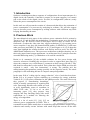
Software is nothing more than a sequence of configurations for an important part of a
digital circuit; the controller. Controller’s purpose, as its name suggests, is to control
part or the whole of the digital circuit. As such, its configuration (software) vastly
affects the power consumption of the circuit.
In this work we will present the creation of a framework that allows the estimation of
power consumption of a processor by analyzing its software. We will also suggest
ways to decrease power consumption by writing software with a different way while
keeping functionality the same.
2. Previous Work
The most historical early papers in the software power estimation field is written by
Tiwari et al. [1] and describes the methodology of estimating power on a 486 with an
analytical way. We heavily relied on this paper and we used its values for our
framework. At about the same time they suggest techniques [2] for creating power
aware compilers. Later they did characterization studies on SPARClite [3] and some
other processors and DSPs [4]. Hasegawa et al. [5] and Segars et al. [6] at about the
same time highlight the relation between code density and low power for SH3 and
ARM/Thumb instruction sets. Their processor architecture techniques that they use in
their early papers latter became mainstream. At architectural level, principles from the
extended addressing mode [7] of Kalambur et Al could be considered.
Benini et al. summarize [8] the available solutions for low power design with
extensive references. Probably this was done in order to support their later paper [9]
where they compare very well different C constructs on their energy efficiency. They
talk about recursion that we also studied. Their claim that “On the ARM processor the
overhead is small - only four instructions” is wrong. The problem isn’t the
calling/returning but parameter passing (possibly via the expensive stack). The whole
paragraph is a bit misleading because it compares unequal algorithms.
In the same field of “coding tips for energy reduction” a lot of work has been done.
Metha [10] et al. propose register relabeling as a technique for energy reduction.
Vishal et Al. [11] do power estimation for the ARM processor. The most effective tip
they propose is “transforming branchings”
which is actually synonymous to repairing bad
code. Decreasing function calls (which we used
as well) significantly seems to contribute in
ARM 32-bit code. Li Lai et al. on their
interesting paper [12], they propose loop
merging and loop unrolling along with scalar
replacement as a method for reducing the
energy of an algorithm.
There is a lot of work [13], [14], [15] on
software power optimization on DPSs. This is
reasonable because DSPs usually have to retain their high performance despite energy
reduction and usually execute software with small loops that execute all the time
2
(easier to optimize) instead of general purpose control-oriented code. A software
power reduction technique that could fit very well DSPs needs is that of the energyquality (E-Q) factor presented by Sinha et Al [16]. By using different algorithms or by
simply changing the order of calculations one can have acceptable accuracy with a
minimum number of iterations in arithmetic calculations as the previous figure shows.
If there is enough power, you continue the calculation and get extra accuracy. In noncritical applications like an mp3 player you can trade-off quality with energy to
prologue battery life. They successfully apply this technique for a Microsensor Node
[17].
Brandolese et Al [18] give models of power consumption of software in different
levels of abstraction and as a result with different level of accuracy. They also present
[19] some abstract models based on instruction decomposition in functions based on
their earlier work [20]. The final model includes the inter-instruction effects and is
supposed to be accurate enough. They report to have assembly listings in the order of
107 – 108 lines, which is actually a bottleneck in the whole power estimation process.
After the buzz of the first period, simplicity and efficiency are always the values that
survive. Russell et al. [21] in their brilliant paper verify that the simplest and most
efficient is also accurate. Assuming constant power and just calculating the time is
enough to give energy estimations with 8% of accuracy. This is very important and
can be verified from our work as well. If we haven’t assumed different currents for
each instruction, but we used just a constant current value, small differences in the
results would be noticed. The most important parameter in software power estimation
is time. Much later Sinha et al. [22] used the same assumption to develop JouleTrack,
a web-based power estimation application for StrongARM processors. They also
applied the same principles [23] later to profile an operating system. They highlight
the importance of system function calls which we also verify that are very important
and if overlooked, only wrong conclusions can be drawn. Just estimating the energy
required by malloc could be the subject of a thesis.
Nikolaidis et Al. [24] came late. At their paper we can see how dirty, the work of
estimating software energy can be. They were forced to decode from binary
instructions available from traces of the ARM debugger. The good point is that model
both the core and the memory. Now that they had done it “the hard way” they might
consider taking binary traces directly from the bus [25].
In the System on Chip era new problems arise. Marcello et Al. in their very good
paper [26] show how heterogeneous tools can be used together for software/hardware
power co-estimate. The important about this paper is that they focus on the industry’s
need of both reasonable accuracy but also fast execution time of simulation which is
important when (and it’s always the case) the power estimation is part of an iterative
refinement process. They also give an important literature review on current SOC
power estimation research. Vijaykrishnan et Al. [27] present their SimplePower, one
of the best power estimating tools available at the moment in terms of accuracy and
execution speed. Wehmeyer et Al. [28] propose register file size design space
exploration in order to meet both energy and area budget. Hung-Ming et Al. [29]
summarize what we need to make practically power efficient software development:
1. Use a power-aware compiler
3
2. Establish a set of coding guidelines based on system’s characteristics, and let
the programmers write this way.
3. Collaborate the characteristics of application software such as load with
hardware to dynamically adjust the system processing performance.
Sometimes researchers try to hard in their area and loose the big picture. Gurumurthi
Et al. [30] bring us back to reality with some interesting system-level perspectives.
They rate the power consuming elements of a computer with the following way:
1. “The disk is the single largest consumer of power accounting for 34% of the
system power.”
2. After that comes “clock distribution and generation network and the on-chip
first level instruction cache”
3. “The memory subsystem has a higher average power than the processor core”
The most power consuming parts are more likely to give better energy saving with
least effort. A 3% power reduction in a disk is orders of magnitude better than a 3%
power reduction on a processor’s core. In an mp3 player I suspect that most of the
energy is spent in the analog subsystem. Using cheap Delta-Sigma D/As who operate
in large frequency and with full voltage swing may be more power consuming than
the expensive R-2R D/As. Matching headphones typical resistance with amplifier’s
output resistance and using more efficient headphones (more dB/mV) will be
beneficial as well.
From a software perspective, they observe that the user mode is the most power
consuming (because of the various protection schemes) but the kernel mode consumes
15% of system’s energy due to frequent calls. Over 5% of system’s energy is
consumed in idle mode. Because nothing is being done in that time, a power down
mode could be used instead.
Finally, Hu et Al. [31] give a detailed overview of the latest software power
optimization techniques including techniques for processors with reconfigurable
resources (e.g. reconfigurable caches). They also give an example of one of the few
cases where faster program doesn’t mean less power consumption (compiler-guided
speculative cache prefetching).
4
2. Powprof: Our power estimation framework
2.1 Instruction traces
2.1.1 Tools
In order to estimate power in a platform one thing that is necessary is instruction
traces. Many open source profilers were tested but most of them didn’t provide the
functionality we wanted.
gprof1, the GNU profiler provides information only for the number of calls on
functions (gprof’s internatl operation can be found here2). PIN3 is useful but it doesn’t
provide disassembly of the instructions out of the box. gcov4, the GNU coverage tool
was much closer to what we needed. It provided the number of times each C line was
executed. With a closer look at its source code, it was clear that it was more complex
than we needed in order to be cross-platform. Additionally, by looking at the source
code it generated, it was obvious that the profile files it generated weren’t suitable for
our needs, because they were directed towards profiling C code. For example for a
conditional branch of C with multiple conditions like if (a==0 && b==0), it would
probe just if the branch is taken or not while in assembly this condition translates to
two branches. The second one didn’t get profiled.
2.1.2 Bochs
“Bochs is a highly portable open source IA-32 (x86) PC emulator written in C++, that
runs on most popular platforms. It includes emulation of the Intel x86 CPU, common
I/O devices, and a custom BIOS. Currently, Bochs can be compiled to emulate a 386,
486, Pentium, Pentium Pro or AMD64 CPU, including optional MMX, SSE, SSE2
and 3DNow! instructions.”5.
Bochs is a very accurate and it allows instruction level emulation of arbitrary
programs as complicated as operating systems. Operating systems like dos (FreeDOS)
and linux (DLX linux) are available as images from Bochs’ web site and have been
tested successfully but they don’t provide compiler internally. Bohcs can also be used
for debugging BIOS implementations.
Bochs provides a powerful instrumentation facility. The problem is that it’s not as
complete as I expected.
Problem 1: It’s enabled by default and doesn’t turn off. There is so much time
consuming tracing that doesn’t allow FreeDOS to boot in a reasonable amount of
time.
Solution: I modified instrument.cc and instrument.h by adding two missing functions:
void bx_instr_start() {
active = 1;
}
1
http://www.cs.utah.edu/dept/old/texinfo/as/gprof_toc.html
http://www.informatik.uni-hamburg.de/RZ/software/gnu/gcc/gprof_9.html
3
http://rogue.colorado.edu/Pin/docs/pin-2.0-1061-gcc.3.2-ia32/html/
4
http://gcc.gnu.org/onlinedocs/gcc-3.0/gcc_8.html
5
http://bochs.sourceforge.net/
2
5
void bx_instr_stop() {
active = 0;
}
and turned instrumentation off by default:
static bx_bool active = 0;
Problem 2: “instrument stop” instruction doesn’t work. You can start probing a
program but you can’t stop.
Solution: This is a bug of bochs. I quickly fixed it by changing the instruction to
“instrument stops” by modifying “bx_debug/dbg_main.cc”. I submitted a detailed bug
report to bochs’ forum.
2.1.3 Our approach
A set of Perl scripts were written that take x86 assembly source code from the gcc –S
and analyze it. When program flow changes are detected, a small chunk of code is
interleaved that increases the appropriate profiling counter. At the exit points of
main() a special function call is also called. This function takes these profiling
counters and writes them to a regular text file. The profiling counters are 64 bits long.
The assembly listing for the function that writes the counters to the file were created
with gcc and modified by hand. The whole idea was inspired by the way gcov works.
The second Perl script takes the profile file and the original assembly file and creates
a file of the powest format (see Appendix A.5) that is ready to be used from the rest of
the flow. The main advantage of this technique is that it’s extremely fast because it
runs at native system’s speed. It even allows probing of optimized assembly files (e.g.
gcc –O3). The main disadvantage is that it doesn’t trace system calls and is limited to
a single assembly file.
Another alternative for creating instruction traces is Bochs Emulator that we
described above. We have implemented instrumentation modules that create powest
formatted files directly. Internally we use STL’s map object to minimize the amount
of memory that is needed to store profiling data. By using the instrument start,
instrument stops, instrument reset and instrument print commands we can control the
instrumentation functionality of bochs (see Appendix A.7). The main disadvantage of
bochs is that it’s too slow. Its main advantage and disadvantage at the same time is
that it’s too accurate meaning that it gives realistic instruction traces, including
operating system’s and library call’s overhead. Note that no source code is needed in
order to estimate the energy of a program with blochs.
6
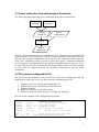
2.3 Power estimation flow with powprof framework
The following figure shows the power estimation flow with our framework.
Perl binary
profiling
Bochs
emulator
powest
format file
powest
configuration
powest
Power
estimations
We have already discussed the two instruction traces’ alternatives, perl profiling and
bochs emulator. After using them, we have a powest formatted instruction trace file.
This file and a powest configuration file are given to the powest tool that creates the
final power estimation results. It must be noted that pwoest formatted instruction
traces and powest configuration files are platform dependant but powest is not. It can
be used with any processor or instruction format like binary, Intel or AT&T assembly
or even more be integrated inside any profiling framework to provide power
estimations.
2.4 The powest configuration file
The real power and flexibility of the powest tool relies on its configuration file. By
modifying its entries one can re-use the powest for estimating power on:
1.
2.
3.
4.
5.
Different processor with the same instruction set
Different processors with different instruction sets
Different systems
Different compilers or assembly notions.
Different operation modes in terms of voltage and frequency
We can see the example of the configuration file bellow.
Comment: All values in mA.
#config
#config
#config
#config
#config
static
volt 3.3
freq 133
dcurre
dclock
push.*
pop.* 428
451
4
100
100 mA static current
3.3V power supply
Frequency in MHz
400.0 Default cost 400mA
2
Default cost 2 clock cycles
1
stack opperations Push functions
stack opperations Pop functions
7
(mov|add|adc|sub|sbb|xor|and|or|cmp|test|xchg).*\$[^,]+,[^%]*%.* 300
2
Arithmetic operations
Arithmetic
opperations
with
immediate
The configuration file is divided in columns. Each column is separated by its next one
by a tab (\t) character. If the first column is empty, it ignores the whole line. If it
contains the #config directive, it tries to parse the following as configuration data.
There are 5 configuration parameters up to now and more may be added on demand:
1.
2.
3.
4.
5.
static
volt
freq
dcurrent
dclock
This is the static current in mA
This the voltage in Volts
This the Frequency in MHz
This is the default current in mA for unknown instructions
This is the default number of clock cycles for unknown instructions
All the parameters are doubles. Even the clock cycles are doubles in powest because
they usually represent mean values. The rest of columns on a #config line are
comments and are not being considered.
If the first column is not empty or #config then we have an instruction line. Every
such line represents a set of instructions. The first column in an instruction line is a
regular expression that matches the specified instruction. A good starting point for
someone who wants to learn regular expressions is wikipedia6. So, for example
“push.*” matches the push instruction followed by anything and the cryptic…
(mov|add|adc|sub|sbb|xor|and|or|cmp|test|xchg).*\$[^,]+,[^%]*%.*
matches all the instructions listed above that operate on an immediate in AT&T
syntax e.g. mov $4324, %eax or movl $WRONG, %MEANINGLESS. What I want
emphasize is that regular expressions are being used in order to distinguish if a line
contains that given instruction. They are able to verify the correctness of an assembly
line (e.g. saying that the second example is wrong) but I don’t think it would be
extremely beneficial because the code is probably correct if created by a compiler or
another automated way. It would just make the whole procedure slower.
The order matters. Instructions are being checked from top to the bottom and the first
match is being accepted. If you have for example:
push.*
pusha.*
the second instruction will never match anything because the first one matches pusha
as well. The best way to build these regular expressions is to start with a clear
configuration file and add one by one ensuring that each one matches exactly what it
should. The commonly used process of starting with a working example and
modifying isn’t beneficial in this case. Note also that arranging the most often used
instruction patterns first improves average performance.
6
http://en.wikipedia.org/wiki/Regular_expression
8
The second column on an instruction argument is the average current in mA that these
instructions consume. This is a value of double type.
The third column is the number of clock cycles for these instructions. This is also a
double value for the reason explained above.
The total energy of the instruction is being calculated by:
Energy = I instr ⋅ Vcc ⋅ Time = I instr ⋅ Vcc ⋅ Cyclesinstr ⋅ (1 freq )
The fourth column is very important. It is the (optional) class of the instruction.
Instructions can be grouped in classes like “Memory write instructions” or “Flow
control instructions”. At the end of power estimation an energy breakdown of all the
classes appears. This way you can find out where your algorithm lacks of energy
efficiency and optimize it e.g. you may find out that stack operations dominate the
power consumption because of excessive use of functions (poor compiler
performance on inlining). The number of classes is unlimited. A default class named
“other” is always being added and contains unclassified instruction i.e. instructions
that have that column empty or instructions that don’t match any pattern.
If something exists beyond the fourth column it is a comment and doesn’t get
considered.
An unlimited number of instructions is being supported. Instruction classification is a
very important feature and has been implemented with this very flexible way.
The configuration file is being passed as (the first) parameter to powest tool. This
means that someone can have tenths of different configurations for different kinds of
processors, voltages clock frequencies or any other property included on the
configuration. By invoking powest with a different configuration file, one gets the
results for the different conditions without any need of recompilation of the program
or re-acquisition or modification of the (usually expensive to obtain) profiling data.
By using regular expressions and not hard-coding the instructions format on the
binary, we are able to use the same program with a new instruction set (e.g. Sparc,
MIPS) within minutes.
9
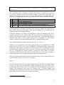
2.5 The powest tool
The powest tool is written in C++. The UML diagram can be seen in the figure
bellow.
As one can easily see powest is nothing more than a wrapper to the PowerEstimator
class. This class does all the work and is autonomous enough to be integrated easily
within each framework. There is no public constructor for the PowerEstimator class
instances of which can be created only by using the static method:
PowerEstmator::createPowerEstimator(). This function returns NULL if the
configuration file passed as parameter doesn’t exist or is faulty. The configuration file
is being parsed to a Configuration Class that includes Instructions and Instruction
classes. PowerEstimator provides three functions; reset(), parseLine() and
printStatistics().
reset() resets its internal accumulators of energy, clock cycles etc. This can be useful
in case you integrate the PowerEstimator to another platform and you want to
measure just a part of a program. You just reset() on the beginning of the part and
printStatistics() at the end.
The parseLine() method should be called each time an instruction is being executed
with the disassembled text as parameter. By calling it instruction’s text is being
compared with the regular expressions from the configuration file. If a match is
found, the energy for the given instruction is being added to the total and its class’s
energy. Otherwise the default energy is being added to the total and the “others”
class’s energy and the instruction is being added to the unknown list.
10
printStatistics() method prints the statistics gathered by the previous procedure. It
prints the total energy, the static energy, the static energy factor (see Appendix B).
Then it prints the breakdown of the energy into instruction classes sorted in reverse
energy consumption order. Finally, if unknown instructions exist, it prints them.
PowerEstmator could be directly integrated on bochs but this wasn’t technically easy
in our development environment (Cygwin) because of some library conflicts. (The
whole bochs is being compiled with the –mno-cygwin flag that prevents the use of the
original Cygwin libraries in order to keep the final executable independent from
Cygwin’s DLLs. Unfortunately regular expression libraries weren’t available on
Cygwin-independent libraries).
2.6 Feature discussion
Our power estimation model allows different average currents for each instruction. As
we will show in the next chapter, this is not extremely important but it allows
somehow more accurate estimations. It also allows approximate modelling of cache
misses, pipeline effects and other inter-instruction effects as described in [1].
11
3. Estimation results
3.1 Energy estimation on mergesort
We have used 3 different implementations of mergesort. A third one that didn’t write
an element to the memory if there was no change was tested but gave worst results
than the original so it didn’t get used. The source code for these three mergesorst can
be found in Appendix D.
msort_original.c
msort_less_calls.c
msort_less_calls_l
ess_writes.c
The original mergesort implementation. Heavily based on
Michael Lamont’s implementation7.
This is a version that has unrolled the 4 last levels of
recursion of mergesort in order to save call overhead. It was
implemented by me, but latter it was found that Knuth8
proposed a similar optimization.
This is the most efficient implementation that has more
complex coding but uses both arrays to half the number of
memory writes.
I would like to comment a little the second one. In
the figure on the right, one can see the way
mergesort works. It breaks the region that has to
be sorted in two and calls itself till it ends to single
numbers. Then it merges the left and right sorted
sub-lists and backtracks. The last e.g. 2 stages get
called n + n/2 times and the merge operation is trivial (nothing or swap) which means
that we just pay the overhead for calling a function for something. This is what is
being attacked by second optimization.
Why mergesort? First of all I believe that it’s the sorting algorithm of the future. It
may be slow but it can be easily parallelized. You just send each sub-list to a different
processor for sorting and then you merge the results. Secondly it is recursive and nontrivial and thus there are a lot of ways to be coded.
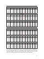
In the tables presented bellow we can see the results obtained by a series of
estimations using profiling and bochs as source of our instruction traces.
The Eest column is the energy estimated by using a constant current of 411 mA instead
of different current for each instruction. For profiling derived data the difference
between the two estimates is 4% on average and 11% worst case. For bochs derived
data the difference is on average 1% and 4% worst case. Obviously we can draw
similar results as in the literature. Using a constant value for current and counting
only the time is not so inaccurate as it sounds.
7
8
http://linux.wku.edu/~lamonml/algor/sort/merge.html (Western Kentucky University)
D. Knuth. The Art of Programming, Vol. 3 (Sorting and Searching). Addison-Wesley, 1973
12
Results from Profiling
Original
n
100
1000
10000
100000
1000000
n
100
1000
10000
100000
1000000
n
100
1000
10000
100000
1000000
Time (s)
0.001
0.006
0.074
0.873
10.100
E (J)
0.001
0.008
0.098
1.160
13.412
Eest (J)
0.001
0.008
0.100
1.185
13.707
Estatic Earith_w
0.000
0.000
0.002
0.003
0.024
0.033
0.288
0.396
3.333
4.657
Less calls
Eflow
0.000
0.002
0.028
0.329
3.828
Earith
0.000
0.001
0.018
0.212
2.496
Earith_r
0.000
0.001
0.012
0.142
1.625
Estack
0.000
0.000
0.004
0.044
0.441
Eother
0.000
0.000
0.004
0.037
0.365
Time (s)
0.000
0.005
0.068
0.813
9.450
E (J)
0.001
0.007
0.090
1.071
12.445
Eest (J) Estatic Earith_w
Eflow
0.001 0.000
0.000 0.000
0.007 0.002
0.002 0.002
0.092 0.022
0.029 0.026
1.103 0.268
0.350 0.313
12.825 3.118
4.110 3.662
Less calls less writes
Earith
0.000
0.001
0.018
0.219
2.589
Earith_r
0.000
0.001
0.011
0.129
1.486
Estack
0.000
0.000
0.002
0.024
0.233
Eother
0.000
0.000
0.004
0.037
0.365
Time (s)
0.000
0.004
0.051
0.604
6.860
E (J)
0.000
0.005
0.067
0.791
8.976
Eest (J)
0.000
0.005
0.069
0.819
9.310
Eflow
0.000
0.002
0.022
0.269
3.088
Earith
0.000
0.001
0.014
0.178
2.075
Earith_r
0.000
0.000
0.005
0.060
0.644
Estack
0.000
0.000
0.003
0.030
0.297
Eother
0.000
0.000
0.004
0.037
0.365
Estatic
0.000
0.001
0.017
0.199
2.264
Earith_w
0.000
0.001
0.018
0.217
2.508
Results from bochs
Original
n
100
500
1000
5000
10000
n
100
500
1000
5000
10000
n
100
500
1000
5000
10000
Time (s)
0.053
0.071
0.102
0.330
0.614
E (J)
0.069
0.094
0.137
0.447
0.833
Eest (J)
0.072
0.096
0.139
0.448
0.833
Estatic Earith_w
0.017
0.009
0.023
0.022
0.034
0.041
0.109
0.183
0.203
0.361
Less calls
Eflow
0.020
0.028
0.042
0.141
0.265
Earith
0.010
0.011
0.013
0.029
0.047
Earith_r
0.006
0.010
0.016
0.068
0.135
Estack
0.024
0.022
0.024
0.026
0.025
Eother
0.001
0.001
0.001
0.001
0.001
Time (s)
0.040
0.052
0.065
0.291
0.618
E (J)
0.053
0.069
0.088
0.395
0.838
Eest (J) Estatic Earith_w
Eflow
0.054 0.013
0.007 0.015
0.071 0.017
0.021 0.021
0.088 0.021
0.037 0.028
0.394 0.096
0.179 0.125
0.838 0.204
0.361 0.265
Less calls less writes
Earith
0.007
0.007
0.006
0.021
0.049
Earith_r
0.005
0.008
0.013
0.063
0.134
Estack
0.017
0.012
0.005
0.006
0.029
Eother
0.001
0.000
0.000
0.000
0.001
Time (s)
0.033
0.045
0.088
0.300
0.587
E (J)
0.043
0.061
0.118
0.407
0.797
Eest (J)
0.044
0.062
0.120
0.407
0.796
Earith
0.006
0.006
0.011
0.023
0.044
Earith_r
0.004
0.007
0.014
0.057
0.113
Estack
0.013
0.009
0.018
0.017
0.026
Eother
0.000
0.000
0.001
0.001
0.001
Estatic
0.011
0.015
0.029
0.099
0.194
Earith_w
0.007
0.020
0.039
0.180
0.358
Eflow
0.013
0.019
0.037
0.130
0.256
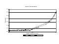
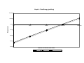
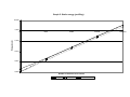
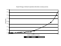
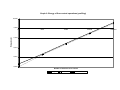
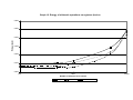
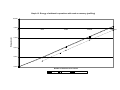
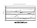
The easiest way to understand those tables is by looking their graphs on Appendix C.
It must be noted that both axes are logarithmic which means that small offsets may
mean great changes. It must also be noted that bochs’ graphs are in the 100-10000
range. We couldn’t go further because emulation times were prohibiting.
13
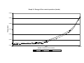
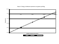
In respect of Total time and energy (Graphs 1-6) we see the same pattern. The second
version of mergesort offers almost no performance benefits while the third one offers
energy reduction of 33% in profiling results and 5% in boch’s results.
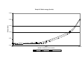
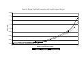
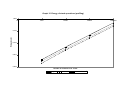
Why this happens is clear in the next graphs (Graphs 7-8) where we see that we have
significantly reduced number of memory writes in profiled results but in bochs’s
results we have almost no difference. Additionally the number of writes doesn’t seem
to be O(n) something like O(an). It must be mentioned however that the third version
of mergesort has approximately half energy consumption on write operations which
means that our optimization was successful.
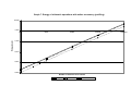
The only interesting thing to note about flow control instructions (Graphs 9-10) is that
in bochs’ version, the second version of mergesort changes in an unexpected way in
respect with the third version of mergesort. The same pattern repeats with arithmetic
operations in registers (Graphs 11-12) and stack operations (Graphs 15-16).
Arithmetic operations with memory read (Graphs 13-14), follow the same pattern
with arithmetic writes and get significantly reduced on the third version.
In profiling stack operations (Graph 15) we can see that the second version is the most
efficient as we expected by having almost half the energy of the original version. This
means that our optimization for reducing the calls was successful. It also means as we
noted before, that the main overhead involved with function calls is not the call/ret but
parameter passing via stack. In the third version of mergesort we have a slight
(although it seems large) increase of 27% on stack operations because of the extra
parameter that is being passed on them (swap). In bochs’ version, the pattern is funny.
No correlation seems to exist and an amplified version of the pattern of flow control
appears.
3.2 Comments on the results
The results are quite the expected for the profiled version and quite unexpected for
bochs’ version. The problem is that what you are going to “pay” as energy to the real
hardware is that of bochs’ version! All these strange patterns in bochs’ version exist
because:
1. DOS compiler is less optimizing than gcc
2. Because of system calls
3. Because of the overhead of the operating system
File loading and unloading the program uses a large number of read/writes and
branches. The number of these calls is independent of ‘n’ and can be larger than the
cost for sorting e.g. 100 numbers.
The most important cause of inconsistency is because of memory allocation/deallocation routines for both loading/unloading the program and program’s needs. The
memory has to be allocated and initialized. Then random number generation has to
take place. Depending on the used algorithm this may add from small to very large
overhead.
14
Random numbers created with naïve random algorithms are not so random. What we
may actually be seeing in many of the energy profiles may be just a result of
correlations between numbers in the array under sort after a certain point (e.g. the
array may be somehow sorted between 1000 elements and 10000 elements). Just one
seed has been used in bochs’ experiment and it’s not checked to have fair statistical
properties.
It takes about half a second to execute the 10000 element’s sorting. During this time a
lot of interrupts to serve even the non-multi-tasking DOS will have taken place.
In conclusion all these high-level effects make the actual energy consumption of a
program running on a real system 10 times more energy consuming than it would be
expected from a first order analysis. The only think we can do given a program file,
without details about the operating system and the libraries is just to tell that it’s more
or less power consuming in comparison with another.
3.3 Power reduction tips
It’s tempting to follow the tradition of each power estimation paper in the past and
provide some power estimation tips. I will do it very briefly because it’s not one of
the aims of this research and because most of the important ideas have already been
highlighted in the literature. I will focus in things that a compiler can’t do, because a
good time-optimizing compiler is also energy efficient in general.
1. Adjust buffer sizes to fit data caches
2. Adjust code size including calling function of loops in order to fit instruction
caches and far jumps are not needed.
3. Allocate the memory on the beginning and manage it yourself. malloc is generally
not supposed to be energy efficient.
4. In general, don’t assume that system calls are energy efficient.
5. Distribute the load. If you can’t power down individual modules, use them in order
to finish earlier or lower the operation frequency. Modern DSPs for example have a
lot of extra features that may remain unused. E.g. setup DMA transfer to send data to
the audio decoder. Don’t pass everything from the CPU.
6. Use interrupts instead of polling for large wait intervals
7. Get to know the compiler. If you make a change e.g. to decrease the number of
writes and you finally end up with more writes then there is some sort of
“misunderstanding” between you and the compiler. See the assembly listings and
understand them to see what’s wrong. After a while you will be able to understand the
compiler and avoid mistakes.
8. Reduce data redundancy (e.g. XML)
9. Know your data and do clever data transformations. For example sometimes storing
an array in a differential form (a[n] = a[n-1]+a[n]) results in small numbers that are
beneficial in a power aspect. You may also be able to transfer more than one such
small number in one memory transaction.
10. Do transformations such as most data have the same bits all the time. It reduces
swing on busses and switching activities. If this means extra time then do a data
transform to save time. E.g. butterfly based FFT, multiply, IFFT instead of FIR with
many taps.
11. Try to compress and de-compress data at runtime. Especially applicable if the
processor has special instructions that help.
15
4. Conclusion
With our program we are able to provide numbers. We provide answer to the question
how much energy is needed to complete a software task. We also provide answer to
the question if a piece of code is more energy efficient than another with the same
functionality.
We give that answer with a piece of software that is portable, configurable, extensible
and relatively fast. Someone with knowledge of regular expression can port it to
another processor. Someone with average C++ knowledge can integrate it to any
profiling framework.
Yet the engineer that uses it has to choose between accuracy and efficiency. Accuracy
is not a matter of current measurement and platform characterization but a matter of
deciding which are the most power consuming hardware (disks, external memories,
buses, caches, cores) and software (operating system, communication protocols,
application) elements of the system and including them in your estimation. Of course
the more items you include, the more inefficient the estimation gets.
So, no, software power estimation is not just a summation. Tracking system’s state is
not an easy job either. Software power estimation is an open problem that has not
been solved both accurately and an efficiently for more than 10 years.
5. References
[1] Vivek Tiwari, Sharad Malik, and Andrew Wolfe: “Power Analysis of Embedded
Software: A First Step Towards Software Power Minimization”, 1994
[2] Vivek Tiwari, Sharad Malik, Andrew Wolfe: “Compilation Techniques for Low
Energy: An Overview”, 1994
[3] V.Tiwari and M.T.C. Lee: “Power analysis of a 32-bit Embedded Microcontroller”, VLSI Design Journal, 1996.
[4] Vivek Tiwari, Sharad Malik, Andrew Wolfe, Mike Tien-Chien Lee: “Instruction
Level Power Analysis and Optimization of Software”, 1996
[5] A. Hasegawa, I.Kawasaki, K.Yamada, S.Yoshioka, S. Kawasaki, and P. Biswas:
"SH3: High code density, low power", IEEE Micro, Dec. 1995.
[6] Keith Clarke Simon Segars and Liam Goudge: “Embedded control problems,
thumb, and the arm7tdmi”, IEEE Micro, 15(5):22--30, October 1995.
[7] A. Kalambur and M. J. Irwin: “An extended addressing mode for low power”,
Proc. Int. Symp. Low Power Electronics Design, Aug. 1997, pp. 208—213
[8] Tajana Simunic, Luca Benini, Giovanni De Micheli: “System-Level Power
Optimization: Techniques and Tools”, 1996
[9] Tajana Simunic, Luca Benini, Giovanni De Micheli: "Energy-Efficient Design of
Battery-Powered Embedded Systems", 1999
[10] H. Mehta, R. Owens, M. Irwin, R. Chen, and D. Ghosh: "Techniques for low
energy software,", Proc. ISLPED Int. Symp. Low Power Electronics and Design,
1997, pp. 72--75.
16
[11] Vishal Dalal, C.P. Ravikumar: “Software Power Optimizations In An Embedded
System”, 2000
[12] Shan Li Lai, E.M.K.; Absar, M.J.: “Minimizing Embedded Software Power
Consumption Through Reduction of Data Memory Access”, 2003
[13] Mike Tien-Chien Lee; Tiwari, V.; Malik, S.; Fujita, M.: “Power analysis and
minimization techniques for embedded DSP software”, 1996
[14] Catherine H. Gebotys, Robert J. Gebotys: “Empirical Comparison of
Algorithmic, Instruction, Architectural Power Prediction Models for High
Performance Embedded DSP”, Proc of ISLPED, 1998
[15] Gebotys, C.H.; Gebotys, R.J.: “Designing for low power in complex embedded
DSP systems”, 1999
[16] Amit Sinha, Alice Wang, Anantha P. Chandrakasan: “Algorithmic Transforms
for Efficient Energy Scalable Computation”, 2000
[17] Rex Min, Manish Bhardwaj, Seong-Hwan Cho, Amit Sinha, Eugene Shih, Alice
Wang, Anantha Chandrakasan: “An Architecture for a Power-Aware Distributed
Microsensor Node”, 2000
[18] C. Brandolese, W. Fomaciari, L. Pomante, F. Salice, D. Sciuto: “A Multi-Level
Strategy for Software Power Estimation”, 2000
[19] Beltrame, G.; Brandolese, C.; Fornaciari, W.; Salice, F.; Sciuto, D.; Trianni, V.:
“An assembly-level execution-time model for pipelined architectures”, 2001
[20] Brandolese, C.; Fornaciari, W.; Salice, F.; Sciuto, D.: “Energy estimation for 32bit microprocessors”, 2000
[21] Russell, J.T.; Jacome M.F.: "Software power estimation and optimization for
high performance, 32-bit embedded processors", 1998
[22] Amit Sinha, Anantha P. Chandrakasan: “JouleTrack A Web Based Tool for
Software Energy Profiling”, Design Automation Conference, 2001
[23] Amit Sinha, Nathan Ickes, Anantha P. Chandrakasan: “Instruction Level and
Operating System Profiling for Energy Exposed Software”, 2003
[24] Nikolaidis, S.; Laopoulos, T.; Chatzigeorgiou, A.: “Developing an environment
for embedded software energy estimation”, 2003
[25] P Bosch, A Carloganu, and D Etiemble: “Complete x86 instruction trace
generation from hardware bus collect”, 1997.
[26] Marcello Lajolo, , Anand Raghunathan, Sujit Dey, and Luciano Lavagno:
“Cosimulation-Based Power Estimation for System-on-Chip Design”, 2002
[27] W. Ye, N. Vijaykrishnan, M. Kandemir, M. J. Irwin: "The Design and Use of
SimplePower: A Cycle-Accurate Energy Estimation Tool", Design Automation
Conference, 2000
[28] Wehmeyer, L.; Jain, M.K.; Steinke, S.; Marwedel, P.; Balakrishnan, M.:
“Analysis of the influence of register file size on energy consumption, code size, and
execution time”, 2001
[29] Hung-Ming Chen; Po-Hung Chen; Tai-Jee Pan; Feipei Lai: “Designing platformbased system power management on a smart tablet appliance”, 2003
[30] Gurumurthi, S.; Sivasubramaniam, A.; Irwin, M.J.; Vijaykrishnan, N.; Kandemir,
M.: “Using Complete Machine Simulation for Software Power Estimation: The
SoftWatt Approach”, 2002
[31] J. Hu, G. Chen, M. Kandemir and N. Vijaykrishnan: “Software Power
Optimisation”, System On Chip: Next Generation Electronics, 2006. pp. 289-316.
17
Appendix A. User manual
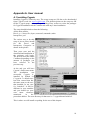
A.1 Installing Cygwin
Installing Cygwin is relatively easy. The setup (setup.exe) file has to be downloaded
from Cygwin’s web site www.cygwin.com. The default options on the setup are OK
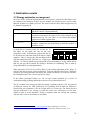
till the “Cygwin setup - select packages” dialog. Here we have to select the packages
for Cygwin installation witch is similar task with any Linux installation.
The setup should include at least the following:
All the base utilities.
Devel: g++, bison, flex, byacc, autoconf, automake, make.
Interpreters: perl
The easiest way to do this
setup is just to select install
for
the
Devel
and
Interpreters Categories as
shown in the picture.
Then press next and the
download and installation of
the packages will begin.
The process will take about
5 minutes depending on the
amount of packages you
have selected in the
previous step.
At the end you will have
Cygwin’s link in start menu.
The
installation
was
successful. Cygwin is
installed by default in
C:\cygwin. A default user
has been created that has
the same name as the user
that installed. In my case
it’s “lookfwd”. It will be
different in your machine
and you should use your
own
name
whenever
mentioned
in
the
procedures bellow. The root directory for that user is: C:\cygwin\home\lookfwd\.
This is where we will install everything for the rest of this chapter.
18
A.2 Installing bochs
Download the latest version of bochs from bochs’ web site
http://bochs.sourceforge.net/. In my case the latest version is bochs-20060518.tar.gz.
Put that file in your root directory (described above). Start Cygwin with the link on
the start menu. Now decompress the archive with the following command:
$ tar –xzf bochs-20060518.tar.gz
Download my framework’s package archive: swcost.tar.gz. Put it in your root
directory and then untar it with the following command.
$ tar –xzf swcost.tar.gz
This creates a swcost directory in your machine. Therein there are some updates to the
original bochs release that must be applied before compilation. Do the following:
$ cp swcost/original_bochs_updates/dbg_main.cc bochs20060518/bx_debug/dbg_main.cc
$ cp swcost/original_bochs_updates/instrument.h bochs20060518/instrument/example0/instrument.h
$ cp swcost/original_bochs_updates/instrument.cc bochs20060518/instrument/example0/instrument.cc
Now we are ready to compile bochs. Goto bochs’ directory
$ cd ~/bochs-20060518
Compile bochs from the source code with the following commands. Configuration
will take about 4 minutes and make will take about 8 minutes.
$ configure --enable-debugger --enable-disasm --enableinstrumentation="instrument/example0" --enable-vbe --enable-clgd54xx
--enable-icache
$ make
$ make install
The installation of bochs is complete.
A.3 Your first bochs session
We can now test bochs with the following procedure. In my swcost directory, there
exists a FreeDOS version from bochs’ web-site (slightly modified). Other operating
systems (like dlxlinux) can be downloaded and tested but this one is already
configured and will work straight out of the bochs! Go to the freedos-img directory
and run bochs.
$ cd ~/swcost/freedos-img/
$ bochs
IMPORTANT NOTE: If you’ve installed Cygwin in a directory other than C:\cygwin,
you will have to modify the following two lines of the bochsrc file in that directory.
romimage: file="C:\cygwin\usr\local\share\bochs\BIOS-bochs-latest",
address=0xf0000
19
vgaromimage:
latest"
file="C:\cygwin\usr\local\share\bochs\VGABIOS-lgpl-
Now I assume that you have initiated a bochs session and you see something like this:
Please choose one: [5]
Press enter. After a while bochs console appears as it can be seen in the figure bellow.
Bochs’ console
Cygwin’s console
So now we have two consoles. The one is Cygwin’s console and the other one is
bochs’ console. This terminology will be used for the rest of the chapter. The
simulation is initially paused. So go in Cygwin’s console and enter ‘c’ <enter> to
continue the simulation. You will now see a familiar DOS booting prompt on bochs’
console. Press enter two times. You will now end up with a DOS prompt: C:\ in
bochs’ console. Goto progs directory.
> cd progs
This is where I’ve put some sorting executables: msor, mslc and mslclw
corresponding to the three versions of the sorting functions. Run one of them:
> msor 200
A “Done.” must appear that indicates that the sorting is complete. Because these
programs are used for instrumentation, detailed messages are not included to
minimize I/O overhead.
20
Now go to Cygwin’s console and press Ctrl+C. Now we are in debug mode and
boch’s console is inactive. Start the instrumentation facility and continue the
simulation by entering c.
<bochs:2> instrument start
<bochs:3> c
You will immediately see a listing of the assembly code that bochs is running just and
only to prompt for your key-press on your DOS window. You may now begin to
realize that instrumentation and power estimation is really much more complex task
than you thought.
Press Ctrl+C again in Cygwin’s console. Stop the instrumentation and continue.
<bochs:4> instrument stops
<bochs:5> c
This feature didn’t actually work in the original bochs’ and was one of the
modifications done with the patch files we used before. Now press the power button
in bochs’ console window. This will end your bochs session. Congratulations, you
have successfully run your first session on bochs’ virtual processor.
For more information about bochs consult the bochs documentation at
http://bochs.sourceforge.net/.
A.4 Installing powprof framework
You have already installed my powprof framework by unpacking the swcost archive.
I will provide some more details in case that you want to modify or extend the
framework. You can safely skip this chapter if you are interested only on using the
framework.
The frameword directory is the swcost directory.
Here you will find the source code of the powest power estimator. This consists of
three files: PowerEstimator.cc, PowerEstimator.hh and powest.cc. The first
two files are completely self contained and it’s extremely easy to integrate them to
another profiling suite. You can compile them with the following command.
$ g++ -O3 powest.cc PowerEstimator.cc -o powest
This generates “powest.exe” on Cygwin platform or “powest” on most unix
platforms. This powest tool uses can parse files with listings of assembly instructions
and their frequency of usage in the following “powest format”:
|------ 19 characters --|- tab -|--------- Instruction --------|
180000
mov (%eax), %ebx
222
jmp L3
This format is powest.cc - specific. The PowerEstimator.cc provides a generic class.
21
There are two demo configuration files: gcc_x86.powconf and bochs_x86.powconf.
The first one is being used for the gcc AT&T assembly syntax and the second one is
being used for bochs’ disassembled instruction syntax.
There are also two very important perl scripts that are the backbone of the powprof
framework. These are: add_probes.pl and back_annotate_probes.pl.
add_probes.pl takes as parameter a .s assembly file as created with gcc if a
compilation with the –S option and creates a _probed.s file that has a small probe
function each time the flow control may changes within the file; labels (entry points)
and jumps/rets (exit points). At the end(s) of the main routine, a call to a special
assembly function (_prof_print_prof_data) is being added to write probing results
to a file named prof_data.txt. All these functions are assembly functions and are
highly likely to change on a port to another instruction set.
The back_annotate_probes.pl takes the original .s file and the profiling result
(prof_data.txt) and creates a file in the powest format with the frequency of
occurrence for each instruction. This is very similar to the add_probes.pl and is also
highly probable to change on a port to another instruction set.
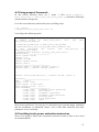
The powprof.sh file is a bash script that executes all the actions required to profile a
.c source file. We will comment its procedure because it’s very important to
understand the flow of data through the tools.
> gcc "$1.c" $3 –S
This compiles the .c file using as parameters the third command line parameters
(usually a –Ox parameter that will give the optimization level) and by using the –S
switch creates an assembly listing of the program.
> add_probes.pl "$1.s" > "$1_probed.s"
This script adds probes to the places that the flow changes within the assembly
program.
> gcc "$1_probed.s" -o "$1_probed"
Then we compile this modified assembly program.
> `$1_probed $2`
And we execute it with the second command line parameter as parameter. In the
sorting cases, this is the number of elements to be sorted.
> back_annotate_probes.pl "$1.s" prof_data.txt > "$1_back.s"
This back annotates profiling data back to the original assembly level file. The
generated file is in powest format.
> powest gcc_x86.powconf "$1_back.s"
At the end we run powest and this gives us the actual numbers about the energy
consumption with the given parameters.
This modular structure of the powprof framework gives it so much flexibility and the
ability to easily be modified to other platforms and execution environments with
minimum coding effort.
22
A.5 Using powprof framework
In the swcost directory there are 3 demo .c files (msort_original.c,
msort_less_calls.c, msort_less_calls_less_writes.c) with three differently
coded versions of mergesort.
Go to the swcost directory and run the power profiling script.
$ cd ~/swcost
$ powprof.sh msort_less_calls 1000 -O3
You will get the following result:
>> Creating msort_less_calls.s file, optimization level: -O3
>>
Adding
probes
to
msort_less_calls.s
file.
New
msort_less_calls_probed.s
>> Compiling probed file to msort_less_calls_probed
>> Executing msort_less_calls_probed with parameter 1000
>>
Back
annotating
the
results
from
prof_data.txt
msort_less_calls_back.s
>> Running power estimator on msort_less_calls_back.s
Configuration______________________
Static current 100 mA
Voltage 3.3 V
Frquency 133 MHz
Default current 400 mA
Default clock 2
___________________________________
Pattern: pusha.*, current: 451 mA, cycles: 9
Pattern: popa.*, current: 428 mA, cycles: 9
file:
to
...
Pattern: (rol|ror|sal|shl|sar).*, current: 300 mA, cycles: 4
Statistics_________________________
time:
0.0054 s
energy: 0.0071 Joule
static energy: 0.0018 Joule
static energy factor:
25.0 %
Class breakdown____________________
1
0.0022 Joule
arithmetic write operations
2
0.0020 Joule
flow control
3
0.0014 Joule
arithmetic operations
4
0.0009 Joule
arithmetic read operations
5
0.0004 Joule
floating point
6
0.0002 Joule
stack opperations
7
0.0000 Joule
other
How easier could it be? You just give it a file and it gives you the energy estimation
and the breakdown in instruction classes. Test it with other functions and other
parameters to see it working.
A.6 Installing bochs power estimation extensions
Now we are going to install some extensions to bochs in order to allow it to be used
for instrumentation.
23
cp -r ~/swcost/bochs_powest/* ~/bochs-20060518/instrument/
Now we go back to bochs’ directory and clean the old configuration.
$ cd ~/bochs-20060518
$ make dist-clean
Then we re-run the configuration and make process with slightly different parameters.
$ configure --enable-debugger --enable-disasm --enableinstrumentation="instrument/powest" --enable-vbe --enable-clgd54xx -enable-icache
$ make
$ make install
The re-installation of bochs is now complete.
A.7 Using bochs for accurate system-aware power estimation
Let’s go back to our FreeDOS example. We will go through a process similar to the
one of chapter A.3.
$ cd ~/swcost/freedos-img/
$ bochs
Press Enter and c <enter> in Cygwin’s console. Then press two enters in bochs’
console. Then goto progs directory by typing cd progs on bochs’ console. Now write
in bochs’ console and DON’T press enter.
> msor 200
Press Ctrl+C on Cygwin’s console. You will see something like this:
Next at t=77192901
(0) [0x000f4c23] f000:4c23 (unk. ctxt): mov ax, 0x0082
; b88200
Start the instrumentation.
<bochs:2> instrument start
<bochs:3> c
By pressing enter after c go quickly to bochs’ console and press enter. This way you
don’t account much of system’s overhead before program’s execution start. Wait until
you see “Done.”. Then go quickly to Cygwin’s console and press Ctrl+C. You will se
something like this:
Next at t=56309027
(0) [0x000016ea] 0060:10ea (unk. ctxt): mov word ptr ss:[bp+0xfffc],
0x0000 ; c746fc0000
Now write the following instruction to force instrumentation file’s printing.
<bochs:4> instrument print
24
Profile data successfully saved in file "probe.stat"
An probling file named “probe.stat” has been saved in the local directory
(~/swcost/freedos-img/). This is already in pwoest format. An example of that file can
be seen in the figure bellow.
350
29
600
600
600
3
adc
adc
adc
adc
adc
adc
ah,
ax,
ax,
ax,
ax,
cx,
0x00
word
word
word
word
cx
ptr
ptr
ptr
ptr
ds:[bx+0x1b7a]
ss:[bp+0xfffa]
ss:[bp+0xfffc]
ss:[bp+0xfffe]
Then you type the following instructions:
<bochs:5> instrument stops
<bochs:6> instrument reset
<bochs:7> c
And the DOS execution continues as usually. The instrument reset command resets
the internal structures of our boch’s instrumentation module. This way, you can now
continue re-applying the above procedure to probe another program or to probe the
same program with other parameters. Once you are done, press the Power button on
bochs’ window to end the bochs session.
Be careful. Each time you execute “instrument print”, the old “probe.stat” file (if
exists) gets overridden which means that if you need it you should have already
renamed it.
We have some sample files of our execution probing in the ~/swcost/statistics files/.
We will see how the process continues by using one of them. So we assume that you
have one of your probe “.stat” files from bochs. You then go to the powprof folder by
typing:
$ cd ~/swcost/
Then you run the powest tool directly (without using powprof.sh) by typing:
$ powest bochs_x86.powconf statistics\ files/probe_msor_1000.stat
As we said above, bochs’ “.stat” files are already in powest format so no conversion is
needed. Note also that we now use the bochs_x86.powconf that has the configuration
for bochs’ style disassembly listings and includes more instructions that appear in a
realistic system that runs operating system and library functions as well.
The results that you will get are similar to the following:
Configuration______________________
Static current 100 mA
Voltage 3.3 V
Frquency 133 MHz
Default current 400 mA
Default clock 2
25
___________________________________
Pattern: pusha.*, current: 451 mA, cycles: 9
Pattern: popa.*, current: 428 mA, cycles: 9
...
Pattern: stos.*, current: 451 mA, cycles: 5
Statistics_________________________
time:
0.1023 s
energy: 0.1366 Joule
static energy: 0.0338 Joule
static energy factor:
24.7 %
Class breakdown____________________
1
0.0416 Joule
flow control
2
0.0405 Joule
arithmetic write operations
3
0.0244 Joule
stack opperations
4
0.0164 Joule
arithmetic read operations
5
0.0131 Joule
arithmetic operations
6
0.0007 Joule
other
As you can see bochs gives much higher energy consumption even for simple
programs. This is true. Just for loading executable’s file to the memory and printing
the “Done.” message requires a lot of operations, maybe more than sorting.
A.8 Compiling your own programs for FreeDOS
In the swcost/tools/ folders you will find all the tools you need to compile and run
your own programs in this FreeDOS environment. I use the freeware HI-TECH
Pacific DOS compiler to compile programs for FreeDOS.
The functions have to be de-unixified in order to be compiled successfully with
pacific compiler. More specifically the time.h library doesn’t exist and as a result, we
use a constant to initialize our random routine. The three DOS compatible source files
can be found in the swcost\dos_versions directory and are msor.c, mslc.c and
mslclw.c. Note that these should have the old 8.3 DOS filename format in order to
work with FreeDOS. In the same directory are the corresponding executables and the
executables which start with “o” which are cygwin executables for the same
algorithms. The latter can’t be executed in the FreeDOS environment.
Back to our compilation process. To compile a program you use the Pacific C
compiler picc.exe. Assuming that you are in the binary directory of the pacific
compiler (e.g. C:\pacific\bin) and that your source file is there as well, you write e.g.:
pacc.exe msor.c
This creates msor.exe. Now that you have the executable the problem is that you have
to insert into bochs’ disk image in order to be able to run it with FreeDOS. To do it,
we use a Japanese program, DiskExplorer9 that can also be found in the tools
directory. We open c.img image file (on C:\cygwin\home\lookfwd\swcost\freedos.img\) as “vmware plain disk” and add the files via the graphical interface. Note
that a large part of the user interface is written in Japanese, so good luck!
9
http://hp.vector.co.jp/authors/VA013937/editdisk/index_e.html
26
A.9 Your way through
This tutorial has provided you with everything you need to start using the powprof
framework to estimate power consumption of programs. The problem that you may
have now is that you have too many options. To summarize, there are two main ways
to use the powprof framework.
If you want to optimize the power of your own small algorithmic functions then you
will probably work with powprof.sh to have very easy, fast and noise-free power
estimation. Limitations of this option are that up to the moment it works with single
file programs and of course it doesn’t profile anything that isn’t included in that single
file e.g. library calls. Both of them are not major drawbacks but limit its usage to
small algorithmic functions as described above.
If you want more detailed system-aware power estimation then you will probably use
bochs. If you want to use FreeDOS you can use Hitech’s Pacific dos compiler or any
other DOS compiler or assembler. Of course this limits you a lot and who develops
for DOS anymore anyway? The reason I used this option is because I wanted a quick
and easy evaluation platform for our bochs extensions. You can use bochs with linux
(http://bochs.sourceforge.net/diskimages.html)
or
windows
(http://www.psyon.org/projects/bochs-win32/) distributions. You can also use any
compiler tool you want. The only problem that exists in this option is simulation’s
performance. You can overcome this problem by applying instrumentation only on
the time it’s needed. Further development (e.g. indexing of instructions’ regex’s) and
integration inside bochs of the PowerEstimator class can drastically improve the
performance as well. This is a really powerful option of simulation that can give very
realistic values for the power consumption including operating system’s and library
calls’ overhead.
If you want to port the powprof framework to another instruction set or architecture
you can do it easily by modifying two perl scripts and a configuration file. (Refer to
chapter A.4). The fact that powprof.sh is based on gcc, which has already been ported
to many platforms and supports cross-compiling, makes porting significantly easier.
If you want to extend powprof framework to support more options or to include more
things on power estimation you will find it extremely easy. For example to include the
cost of interrupts call PowerEstimator’s parseLine function with a string like
“<interrupts>” as a parameter and add a similar line to the configuration file.
To integrate the PowerEstimator into another profiling environment or another data
flow just study the PowerEstimator class and you will be able to integrate it quickly.
There are certain things that can be done easily and others that can’t. In the later case
you may have to modify the source code.
I hope you found this User Manual useful and inspiring.
Dimitris Kouzis – Loukas
24 May 2006
27
Appendix B. Static power consumption
The main property of static power consumption that makes us consider it separately is
that it doesn’t depend only on the clock cycles of a program but also on clock’s
frequency.
A program executed on a CMOS processor on 1Mhz in 1second requires the same
dynamic (switching) energy with the same program executed in 2 seconds on 500kHz.
The second version requires twice the static energy in comparison to the first one.
Static power consumption is being caused by leakage power on transistors and thus
depends on their state. If we wanted to be extremely precise we would have to go
down to a spice model of a processor. Obviously this is not a reasonable decision in
most of cases. We estimate this with a constant current value that can be measured by
averaging the current, with stopped clocked, for different internal states.
By using “base energy costs” [1] we include the static power consumption in our
measurements. We only have to consider it separately if we want to calculate the
percentage of our energy that gets wasted on leakage. To do this we multiply the total
execution time with the static power and the result is static energy. Then we divide the
static energy with the total energy and we have the static energy factor.
t ⋅i
⋅V
static energy factor (%) = 100 ⋅ total static CC %
Etotal
Obviously the slowest the frequency, the higher the waster static energy is. With the
increasing participation of the leakage power to the total power consumption this may
become an important metric.
Appendix C. Graphs
28
Graph 1. Total time (profiling)
100,000
10,000
Energy (Joule)
1,000
100
1000
10000
100000
0,100
0,010
0,001
0,000
Number of elements to be sorted
original
less calls
less calls & writes
1000000
Graph 2. Total time (bochs)
0,700
0,600
Energy (Joule)
0,500
0,400
0,300
0,200
0,100
0,000
100
1000
10000
Number of elements to be sorted
original
less calls
less calls & writes
Graph 3. Total Energy (profiling)
100,000
10,000
Energy (Joule)
1,000
100
1000
10000
100000
0,100
0,010
0,001
0,000
Number of elements to be sorted
original
less calls
less calls & writes
1000000
Graph 4. Total Energy (bochs)
0,900
0,800
0,700
Energy (Joule)
0,600
0,500
0,400
0,300
0,200
0,100
0,000
100
1000
10000
Number of elements to be sorted
original
less calls
less calls & writes
Graph 5. Static energy (profiling)
10,000
Energy (Joule)
1,000
100
1000
10000
100000
0,100
0,010
0,001
0,000
Number of elements to be sorted
original
less calls
less calls & writes
1000000
Graph 6. Static energy (bochs)
0,250
Energy (Joule)
0,200
0,150
0,100
0,050
0,000
100
1000
10000
Number of elements to be sorted
original
less calls
less calls & writes
Graph 7. Energy of arithmetic operations with writes on memory (profiling)
10,000
Energy (Joule)
1,000
100
1000
10000
100000
0,100
0,010
0,001
0,000
Number of elements to be sorted
original
less calls
less calls & writes
1000000
Graph 8. Energy of arithmetic operations with writes on memory (bochs)
0,400
0,350
0,300
Energy (Joule)
0,250
0,200
0,150
0,100
0,050
0,000
100
1000
10000
Number of elements to be sorted
original
less calls
less calls & writes
Graph 9. Energy of flow control operations (profiling)
10,000
Energy (Joule)
1,000
100
1000
10000
100000
0,100
0,010
0,001
0,000
Number of elements to be sorted
original
less calls
less calls & writes
1000000
Graph 10. Energy of flow control operations (bochs)
0,300
0,250
Energy (Joule)
0,200
0,150
0,100
0,050
0,000
100
1000
10000
Number of elements to be sorted
original
less calls
less calls & writes
Graph 11. Energy of arithmetic operations on registers (profiling)
10,000
Energy (Joule)
1,000
100
1000
10000
100000
0,100
0,010
0,001
0,000
Number of elements to be sorted
original
less calls
less calls & writes
1000000
Graph 12. Energy of arithmetic operations on registers (bochs)
0,060
0,050
Energy (Joule)
0,040
0,030
0,020
0,010
0,000
100
1000
10000
Number of elements to be sorted
original
less calls
less calls & writes
Graph 13. Energy of arithmetic operations with read on memory (profiling)
10,000
Energy (Joule)
1,000
100
1000
10000
100000
0,100
0,010
0,001
0,000
Number of elements to be sorted
original
less calls
less calls & writes
1000000
Graph 14. Energy of arithmetic operations with read on memory (bochs)
0,160
0,140
0,120
Energy (Joule)
0,100
0,080
0,060
0,040
0,020
0,000
100
1000
10000
Number of elements to be sorted
original
less calls
less calls & writes
Graph 15. Energy of stack operations (profiling)
1,000
100
1000
10000
100000
Energy (Joule)
0,100
0,010
0,001
0,000
Number of elements to be sorted
original
less calls
less calls & writes
1000000
Graph 16. Energy of stack operations (bochs)
0,035
0,030
Energy (Joule)
0,025
0,020
0,015
0,010
0,005
0,000
100
1000
10000
Number of elements to be sorted
original
less calls
less calls & writes
Appendix D. Mergesorts’ source code
msort_original.c
#include
#include
#include
#include
#include
<stdio.h>
<stdlib.h>
<time.h>
<string.h>
<sys/time.h>
#define DATA_RANDOM 1
#define DATA_INCREASING_RAMP 2
#define DATA_DECREASING_RAMP 3
// Change this to one of the options from the list above
// to select source data type
#define DATA_TYPE DATA_RANDOM
#define bool int
#define true 1
#define false 0
void Merge(int numbers[], int temp[], int left, int middle, int right) {
int i, leftend, elements, pos;
leftend = middle - 1;
pos = left;
elements = right - left + 1;
while((left <= leftend) && (middle <= right)) {
if(numbers[left] <= numbers[middle]) {
temp[pos] = numbers[left];
pos++;
left++;
}
else {
temp[pos] = numbers[middle];
pos++;
middle++;
}
}
while(left <= leftend) {
temp[pos] = numbers[left];
left++;
pos++;
}
while(middle <= right) {
temp[pos] = numbers[middle];
middle++;
pos++;
}
for(i=0;i<=elements;i++) {
numbers[right] = temp[right];
right--;
}
}
void m_sort_original(int *numbers, int *temp, int left, int right,
depth){
int middle;
if (right > left) {
middle = (right + left) >> 1;
m_sort_original(numbers, temp, left, middle, depth+1);
middle++;
m_sort_original(numbers, temp, middle, right, depth+1);
int
29
Merge(numbers, temp, left, middle, right);
}
}
void Merge_Sort(int *numbers, int size) {
int * temp = (int *)malloc(size * sizeof(int));
m_sort_original(numbers, temp, 0, size-1, 0);
free(temp);
}
void generateData(int *numbers, int type, int size) {
int i;
struct timeval tv;
switch (type) {
case DATA_RANDOM:
if (SEED == -1) {
gettimeofday(&tv, NULL);
srand ( tv.tv_usec );
}
else srand((unsigned int)SEED);
for(i=0;i<size;i++) {
// Better method for generating random numbers according to the man
numbers[i] = 1+(int) (100.0*rand()/(RAND_MAX+1.0));
}
break;
case DATA_INCREASING_RAMP:
for(i=0;i<size;i++) numbers[i] = i;
break;
case DATA_DECREASING_RAMP:
for(i=0;i<size;i++) numbers[i] = size-i;
break;
}
}
void printData(int *numbers, int size, char * message) {
int i;
printf("%s\n", message);
for(i=0;i<size;i++) printf("%d ", numbers[i]);
printf("\n");
}
int main(int argc, char **argv)
{
int i, size;
int* numbers;
int* numbers2;
if (argc < 2) {
printf("Usage m_sort <number of samples>\n");
return;
}
if (sscanf(argv[1], "%d", &size) != 1) {
printf("Expected integer\n");
return;
}
numbers = (int *)malloc(size * sizeof(int));
//
//
generateData(numbers,DATA_TYPE, size);
printData(numbers, size, "Before");
Merge_Sort(numbers, size);
printData(numbers, size, "After");
free(numbers);
}
30
msort_less_calls.c
… the same with msort_original.c with the only change of:
void m_sort(int *numbers, int *temp, int left, int right, int depth) {
int middle;
int dif = right - left;
if(dif > 0) {
if (dif >= 16) {
middle = (right + left) >> 1;
m_sort(numbers, temp, left, middle, depth+1);
middle++;
m_sort(numbers, temp, middle, right, depth+1);
Merge(numbers, temp, left, middle, right);
}
else {
switch (dif) {
case 1:
Merge(numbers, temp, left+0, left+1, left+1);
break;
case 2:
Merge(numbers, temp, left+0, left+1, left+1);
Merge(numbers, temp, left+0, left+2, left+2);
break;
case 3:
Merge(numbers, temp, left+0, left+1, left+1);
Merge(numbers, temp, left+2, left+3, left+3);
Merge(numbers, temp, left+0, left+2, left+3);
break;
case 4:
Merge(numbers, temp, left+0, left+1, left+1);
Merge(numbers, temp, left+0, left+2, left+2);
Merge(numbers, temp, left+3, left+4, left+4);
Merge(numbers, temp, left+0, left+3, left+4);
break;
…
default:
break;
}
}
}
}
msort_less_calls_less_writes.c
… the same with msort_original.c with the only change of:
void Merge(int * numbers, int * temp, int left, int middle, int right, bool
swap) {
int i, leftend, elements, pos;
int * tmp;
leftend = middle - 1;
pos = left;
elements = right - left + 1;
if (swap) {
tmp = temp;
temp = numbers;
numbers = tmp;
}
while((left <= leftend) && (middle <= right)) {
if(numbers[left] <= numbers[middle]) {
31
temp[pos] = numbers[left];
pos++;
left++;
}
else {
temp[pos] = numbers[middle];
pos++;
middle++;
}
}
while(left <= leftend) {
temp[pos] = numbers[left];
left++;
pos++;
}
while(middle <= right) {
temp[pos] = numbers[middle];
middle++;
pos++;
}
}
bool m_sort(int *numbers, int *temp, int left, int right) {
int middle;
bool i_swap = true;
int dif = right - left;
if(dif > 0) {
if (dif >= 16) {
middle = (right + left) >> 1;
m_sort(numbers, temp, left, middle);
middle++;
if (middle < right)
i_swap = m_sort(numbers, temp, middle, right);
Merge(numbers, temp, left, middle, right, i_swap);
}
else {
switch (dif) {
case 1:
Merge(numbers, temp, left+0, left+1, left+1, false);
i_swap = false;
break;
case 2:
Merge(numbers, temp, left+0, left+1, left+1, false);
temp[left+2] = numbers[left+2];
Merge(numbers, temp, left+0, left+2, left+2, true);
i_swap = true;
break;
case 3:
Merge(numbers, temp, left+0, left+1, left+1, false);
Merge(numbers, temp, left+2, left+3, left+3, false);
Merge(numbers, temp, left+0, left+2, left+3, true);
i_swap = true;
break;
…
default:
printf("Bug!");
break;
}
}
}
return !i_swap;
}
32