1
ISSN 1342-2804
Research Reports on
Mathematical and
Computing Sciences
SDPA (SemiDefinite Programming Algorithm)
and SDPA-GMP User’s Manual — Version 7.1.1
Katsuki Fujisawa, Mituhiro Fukuda, Kazuhiro
Kobayashi, Masakazu Kojima, Kazuhide Nakata,
Maho Nakata, and Makoto Yamashita
June 18th 2008, B–448
Department of
Mathematical and
Computing Sciences
Tokyo Institute of Technology
SERIES
B: Operations Research
Research Report B-448
Department of Mathematical and Computing Sciences
Tokyo Institute of Technology
June 2008
SDPA (SemiDefinite Programming Algorithm) and SDPA-GMP
User’s Manual — Version 7.1.1
Katsuki Fujisawa∗1 , Mituhiro Fukuda∗2 , Kazuhiro Kobayashi∗3 , Masakazu Kojima∗4 ,
Kazuhide Nakata∗5 , Maho Nakata∗6 , and Makoto Yamashita∗7
Abstract. The SDPA (SemiDefinite Programming Algorithm) [5] is a software package for solving semidefinite programs (SDPs). It is based on a Mehrotra-type predictor-corrector infeasible
primal-dual interior-point method. The SDPA handles the standard form SDP and its dual. It
is implemented in C++ language utilizing the LAPACK [1] for matrix computations. The SDPA
version 7.1.1 enjoys the following features:
• Efficient method for computing the search directions when the SDP to be solved is large
scale and sparse [4].
• Block diagonal matrix structure and sparse matrix structure are supported for data matrices.
• Sparse or dense Cholesky factorization for the Schur matrix is automatically selected.
• An initial point can be specified.
• Some information on infeasibility of the SDP is provided.
Also we provide the SDPA-GMP, multiple precision arithmetic version of the SDPA via the
GMP Library (the GNU Multiple Precision Arithmetic Library) with additional feature.
• Ultra highly accurate SDP solution by utilizing multiple precision arithmetic.
This manual and the SDPA can be downloaded from the WWW site
http://sdpa.indsys.chuo-u.ac.jp/sdpa/index.html
i
Key words.
∗1
∗2
∗3
∗4
∗5
∗6
∗7
Semidefinite programming, interior-point method, computer software, multiple precision arithmetic
Department of Industrial and Systems Engineering
Chuo University
1-13-27 Kasuga, Bunkyo-ku, Tokyo 112-8551, Japan
Global Edge Institute
Tokyo Institute of Technology
2-12-1-S6-5 Oh-Okayama, Meguro-ku, Tokyo 152-8550, Japan
Center for Logistics Research
National Maritime Research Institute
6-38-1 Shinkawa, Mitaka-shi, Tokyo 181-0004, Japan
Department of Mathematical and Computing Sciences
Tokyo Institute of Technology
2-12-1-W8-29 Oh-Okayama, Meguro-ku, Tokyo 152-8552, Japan
Department of Industrial Engineering and Management
Tokyo Institute of Technology
2-12-1-W9-62, Oh-Okayama, Meguro-ku, Tokyo 152-8552, Japan
Advanced Center for Computing and Communication
RIKEN
2-1 Hirosawa, Wako-shi, Saitama 351-0198, Japan
Department of Mathematical and Computing Sciences
Tokyo Institute of Technology
2-12-1 Oh-Okayama, Meguro-ku, Tokyo 152-8552, Japan
ii
Preface
We are pleased to release a new version 7.1.1 of the SDPA and the SDPA-GMP.
The SDPA 7.1.1 was completely revised from its source code, and there are great performance
improvements on its computational time and memory usage. In particular, it uses and stores less
variables internally, and its overall memory usage is less than half of the previous version. Also
it performs sparse Cholesky factorization when the Schur Complement Matrix is sparse. As a
consequence, the SDPA can efficiently solve SDPs with a large number of block diagonal matrices
or non-negative constraints. Additional, there are some improvements on its numerical stability
due to a better control in the interior-point algorithm.
The differences between this version and the previous version, 6.2.1, are summarized in Section 9.
Finally, we also provide the SDPA-GMP to solve SDPs highly accurately utilizing multiple
precision arithmetic via the GMP Library (the GNU Multiple Precision Arithmetic Library).
Note that the SDPA-GMP is typically several hundred times slower than the SDPA. Details of the
SDPA-GMP are summarized in the Appendix.
We hope that the SDPA and the SDPA-GMP support many researches in various fields. We
also welcome any suggestions and comments that you may have. When you want to contact us,
please send an e-mail to the following address.
iii
Contents
1. Build and Installation
1
1.1
Prerequisites . . . . . . . . . . . . . . . . . . . . . . . . . . . . . . . . . . . . . . .
1
1.2
How to Obtain the Source Code . . . . . . . . . . . . . . . . . . . . . . . . . . . . .
1
1.3
How to Build . . . . . . . . . . . . . . . . . . . . . . . . . . . . . . . . . . . . . . .
2
1.3.1
Fedora 8 and 9 (i386/x86 64/ppc), Red Hat Enterprise Linux (CentOS) 4,
5 (i386/x86 64) . . . . . . . . . . . . . . . . . . . . . . . . . . . . . . . . . .
2
1.3.2
Ubuntu 7.10 Desktop (i386/x86 64) . . . . . . . . . . . . . . . . . . . . . .
2
1.3.3
Vine Linux 4.2 (i386) . . . . . . . . . . . . . . . . . . . . . . . . . . . . . .
2
1.3.4
MacOSX Leopard (Intel/PowerPC) . . . . . . . . . . . . . . . . . . . . . . .
3
1.3.5
MacOSX Tiger (Intel/PowerPC) . . . . . . . . . . . . . . . . . . . . . . . .
3
1.3.6
FreeBSD 6 and 7 . . . . . . . . . . . . . . . . . . . . . . . . . . . . . . . . .
3
1.4
How to Install . . . . . . . . . . . . . . . . . . . . . . . . . . . . . . . . . . . . . . .
4
1.5
Test Run . . . . . . . . . . . . . . . . . . . . . . . . . . . . . . . . . . . . . . . . .
4
1.6
Performance Tuning: Optimized BLAS and LAPACK . . . . . . . . . . . . . . . .
5
1.6.1
Configure Options . . . . . . . . . . . . . . . . . . . . . . . . . . . . . . . .
5
1.6.2
Linking Against ATLAS . . . . . . . . . . . . . . . . . . . . . . . . . . . . .
7
1.6.3
Linking Against GotoBLAS . . . . . . . . . . . . . . . . . . . . . . . . . . .
7
1.6.4
Linking Against Intel Math Kernel Library . . . . . . . . . . . . . . . . . .
7
Performance Tuning: Compiler Options . . . . . . . . . . . . . . . . . . . . . . . .
8
1.7
2. Semidefinite Program
8
2.1
Standard Form SDP and Its Dual . . . . . . . . . . . . . . . . . . . . . . . . . . . .
8
2.2
Example 1 . . . . . . . . . . . . . . . . . . . . . . . . . . . . . . . . . . . . . . . . .
9
2.3
Example 2 . . . . . . . . . . . . . . . . . . . . . . . . . . . . . . . . . . . . . . . . .
9
3. Files Necessary to Execute the SDPA
10
4. Input Data File
11
4.1
“example1.dat” — Input Data File of Example 1 . . . . . . . . . . . . . . . . . . .
11
4.2
“example2.dat” — Input Data File of Example 2 . . . . . . . . . . . . . . . . . . .
11
4.3
Format of the Input Data File . . . . . . . . . . . . . . . . . . . . . . . . . . . . . .
12
4.4
Title and Comments . . . . . . . . . . . . . . . . . . . . . . . . . . . . . . . . . . .
12
4.5
Number of the Primal Variables . . . . . . . . . . . . . . . . . . . . . . . . . . . . .
12
4.6
Number of Blocks and the Block Structure Vector . . . . . . . . . . . . . . . . . .
13
4.7
Constant Vector . . . . . . . . . . . . . . . . . . . . . . . . . . . . . . . . . . . . .
14
4.8
Constraint Matrices . . . . . . . . . . . . . . . . . . . . . . . . . . . . . . . . . . .
14
iv
5. Parameter File
15
6. Output
17
6.1
Execution of the SDPA . . . . . . . . . . . . . . . . . . . . . . . . . . . . . . . . .
17
6.2
Output on the Display . . . . . . . . . . . . . . . . . . . . . . . . . . . . . . . . . .
17
6.3
Output to a File . . . . . . . . . . . . . . . . . . . . . . . . . . . . . . . . . . . . .
20
6.4
Printing DIMACS Errors . . . . . . . . . . . . . . . . . . . . . . . . . . . . . . . .
21
7. Advanced Use of the SDPA
22
7.1
Initial Point . . . . . . . . . . . . . . . . . . . . . . . . . . . . . . . . . . . . . . . .
22
7.2
Sparse Input Data File . . . . . . . . . . . . . . . . . . . . . . . . . . . . . . . . . .
23
7.3
Sparse Initial Point File . . . . . . . . . . . . . . . . . . . . . . . . . . . . . . . . .
24
7.4
Obtaining More Precision on the Approximate Solution . . . . . . . . . . . . . . .
25
7.5
More on Parameter File . . . . . . . . . . . . . . . . . . . . . . . . . . . . . . . . .
25
8. Transformation to the Standard Form of SDP
26
8.1
Inequality Constraints . . . . . . . . . . . . . . . . . . . . . . . . . . . . . . . . . .
26
8.2
Norm Minimization Problem . . . . . . . . . . . . . . . . . . . . . . . . . . . . . .
27
8.3
Linear Matrix Inequality (LMI) . . . . . . . . . . . . . . . . . . . . . . . . . . . . .
28
8.4
SDP Relaxation of the Maximum Cut Problem . . . . . . . . . . . . . . . . . . . .
28
8.5
Choosing Between the Primal and Dual Standard Forms . . . . . . . . . . . . . . .
29
9. For the SDPA 6.2.1 Users
29
A SDPA-GMP
30
A1
Build and Installation . . . . . . . . . . . . . . . . . . . . . . . . . . . . . . . . . .
30
A2
Prerequisites . . . . . . . . . . . . . . . . . . . . . . . . . . . . . . . . . . . . . . .
30
A3
How to Obtain the Source Code . . . . . . . . . . . . . . . . . . . . . . . . . . . . .
31
A4
How to Build . . . . . . . . . . . . . . . . . . . . . . . . . . . . . . . . . . . . . . .
31
A4.1
Fedora 8 and 9 . . . . . . . . . . . . . . . . . . . . . . . . . . . . . . . . . .
31
A4.2
MacOSX . . . . . . . . . . . . . . . . . . . . . . . . . . . . . . . . . . . . .
31
A5
How to Install . . . . . . . . . . . . . . . . . . . . . . . . . . . . . . . . . . . . . . .
32
A6
Test Run . . . . . . . . . . . . . . . . . . . . . . . . . . . . . . . . . . . . . . . . .
32
A7
Parameters . . . . . . . . . . . . . . . . . . . . . . . . . . . . . . . . . . . . . . . .
34
v
1.
Build and Installation
This section describes how to build and install the SDPA. Usually, the SDPA is distributed as
source codes, therefore, users must build it by themselves. We have done build and installation
tests on Fedora 8, 9 (i386/x86 64/ppc), Red Hat Enterprise Linux (CentOS) 4, 5 (i386/x86 64),
Ubuntu 7.10 (i386/x86 64), Vine Linux 4.2 (i386), MacOSX Leopard/Tiger (Intel/PowerPC) and
FreeBSD 6/7. You may also possibly build on other UNIX like platforms and the Windows cygwin
environment.
For better performance, the SDPA should link against optimized Basic Linear Algebra Subprograms (BLAS) and Linear Algebra PACKage (LAPACK). Please refer to the Section 1.6 for
more details.
Alternatively, you can also use our online solver, or check for pre-build binary packages at the
SDPA homepage (see Section 1.2).
1.1
Prerequisites
It is necessary to have at least the following programs installed on your system except for the
MacOSX.
• C, C++ compiler.
• FORTRAN compiler.
• BLAS (http://www.netlib.org/blas/) and LAPACK (http://www.netlib.org/lapack/).
For MacOSX Leopard (Intel/PowerPC), you will need the Xcode 3.0, and you cannot build the
SDPA on the Leopard with Xcode 2.5. For MacOSX Tiger (Intel/PowerPC), you will need either
the Xcode 2.4.1 or the Xcode 2.5.
You can download the Xcode at Apple Developer Connection (http://developer.apple.com/)
at free of charge.
In the following instructions, we install C, C++, FORTRAN compilers, BLAS and LAPACK
and/or Xcode as well. You can skip this part if your system already have them. If not, you may
need root access or administrative privilege to your computer. Please ask your system administrator for installing development tools.
If your system only lacks BLAS and LAPACK, you can build them by yourself without root
privileges and passing appropriate flags at the command line.
1.2
How to Obtain the Source Code
You can obtain the source code following the links at the SDPA homepage:
http://sdpa.indsys.chuo-u.ac.jp/sdpa/index.html
You can find the latest news at about the SDPA at the index.html file.
1
1.3
How to Build
This section describes how to build the SDPA on Fedora 8, 9 (i386/x86 64/ppc), Ubuntu 7.10
(i386/x86 64), Vine Linux 4.2 (i386) MacOSX Intel/PowerPC Leopard (Xcode 3.0)/Tiger (Xcode
2.4.1 and 2.5) and FreeBSD 6/7. We assume that users have a root access via the command “su”
or “sudo”. If you do not have such privileges, please ask your system administrators.
1.3.1
Fedora 8 and 9 (i386/x86 64/ppc), Red Hat Enterprise Linux (CentOS) 4, 5
(i386/x86 64)
To build the SDPA, type the following.
$ bash
$ su
Password:
# yum update glibc glibc-common
# yum install gcc gcc-c++ gcc-gfortran
# yum install lapack lapack-devel blas blas-devel
# yum install atlas atlas-devel
# exit
$ tar xvfz sdpa.7.1.1.src.2008xxxx.tar.gz
$ cd sdpa-7.1.1
$ ./configure
$ make
1.3.2
Ubuntu 7.10 Desktop (i386/x86 64)
To build the SDPA, type the following.
$
$
$
$
$
$
$
$
bash
sudo apt-get install g++ patch
sudo apt-get install lapack3 lapack3-dev
sudo apt-get install atlas3-base atlas3-base-dev
tar xvfz sdpa.7.1.1.src.2008xxxx.tar.gz
cd sdpa-7.1.1
./configure
make
1.3.3
Vine Linux 4.2 (i386)
$ bash
$ su
Modify /etc/apt/sources.list (add the word “extras” between “updates” and “nonfree”) from
rpm
[vine] http://updates.vinelinux.org/apt 4.2/$(ARCH) main plus updates nonfree
rpm-src [vine] http://updates.vinelinux.org/apt 4.2/$(ARCH) main plus updates nonfree
to
2
rpm
[vine] http://updates.vinelinux.org/apt 4.2/$(ARCH) main plus updates extras nonfree
rpm-src [vine] http://updates.vinelinux.org/apt 4.2/$(ARCH) main plus updates extras nonfree
Then, type
#
#
#
#
$
$
$
$
apt-get update
apt-get install gcc-g77
apt-get install lapack lapack-devel blas blas-devel
exit
tar xvfz sdpa.7.1.1.src.2008xxxx.tar.gz
cd sdpa-7.1.1
./configure
make
1.3.4
MacOSX Leopard (Intel/PowerPC)
Download and install the Xcode 3 from Apple Developer Connection (http://developer.apple.com/)
and install it. Note that we support only the Xcode 3 on Leopard. We do not support Leopard
with Xcode 2.5.
$
$
$
$
$
bash
tar xvfz sdpa.7.1.1.src.2008xxxx.tar.gz
cd sdpa-7.1.1
./configure
make
1.3.5
MacOSX Tiger (Intel/PowerPC)
Download and install either the Xcode 2.4.1 or the Xcode 2.5 from Apple Developer Connection.
Then type the following.
$
$
$
$
$
bash
tar xvfz sdpa.7.1.1.src.2008xxxx.tar.gz
cd sdpa-7.1.1
./configure
make
1.3.6
FreeBSD 6 and 7
$ cd /usr/ports
$ su
Password:
# make update
# cd /usr/ports/math/sdpa
# make install
# exit
3
1.4
How to Install
You will find the “sdpa” executable binary file at this point, and you can install it as:
$ su
Password:
# mkdir /usr/local/bin
# cp sdpa /usr/local/bin
# chmod 777 /usr/local/bin/sdpa
or you can install it to your favorite directory.
$ mkdir /home/nakata/bin
$ cp sdpa /home/nakata/bin
1.5
Test Run
Before using the SDPA, type “sdpa” and make sure that the following message will be displayed.
$ sdpa
SDPA start at
Tue Jan 22 15:28:59 2008
*** Please assign data file and output file.***
---- option type 1 -----------sdpa DataFile OutputFile [InitialPtFile] [-pt parameters]
parameters = 0 default, 1 aggressive, 2 stable
example1-1: sdpa example1.dat example1.result
example1-2: sdpa example1.dat-s example1.result
example1-3: sdpa example1.dat example1.result example1.ini
example1-4: sdpa example1.dat example1.result -pt 2
---- option type 2 -----------sdpa [option filename]+
-dd : data dense :: -ds : data sparse
-id : init dense :: -is : init sparse
-o : output
:: -p : parameter
-pt : parameters , 0 default, 1 aggressive
2 stable
example2-1: sdpa -o example1.result -dd example1.dat
example2-2: sdpa -ds example1.dat-s -o example2.result -p param.sdpa
example2-3: sdpa -ds example1.dat-s -o example3.result -pt 2
Let us solve the SDP “example1.dat-s”.
$ sdpa -ds example1.dat-s -o example1.out
SDPA start at
Fri Dec 7 18:30:56 2007
data
is example1.dat-s : sparse
parameter is ./param.sdpa
out
is example1.out
4
DENSE computations
mu
thetaP
0 1.0e+04 1.0e+00
1 1.6e+03 0.0e+00
2 1.7e+02 2.3e-16
3 1.8e+01 2.3e-16
4 1.9e+00 2.6e-16
5 1.9e-01 2.6e-16
6 1.9e-02 2.5e-16
7 1.9e-03 2.6e-16
8 1.9e-04 2.5e-16
9 1.9e-05 2.7e-16
10 1.9e-06 2.6e-16
thetaD
1.0e+00
9.4e-02
3.6e-03
1.5e-17
1.5e-17
3.0e-17
1.6e-15
2.2e-17
1.5e-17
7.5e-18
5.0e-16
objP
-0.00e+00
+8.39e+02
+1.96e+02
-6.84e+00
-3.81e+01
-4.15e+01
-4.19e+01
-4.19e+01
-4.19e+01
-4.19e+01
-4.19e+01
objD
+1.20e+03
+7.51e+01
-3.74e+01
-4.19e+01
-4.19e+01
-4.19e+01
-4.19e+01
-4.19e+01
-4.19e+01
-4.19e+01
-4.19e+01
alphaP
1.0e+00
2.3e+00
1.3e+00
9.9e-01
1.0e-00
1.0e-00
1.0e-00
1.0e-00
1.0e-00
1.0e-00
1.0e-00
alphaD
9.1e-01
9.6e-01
1.0e+00
9.9e-01
1.0e-00
9.0e+01
1.0e-00
1.0e-00
1.0e-00
9.0e+01
9.0e+01
beta
2.00e-01
2.00e-01
2.00e-01
1.00e-01
1.00e-01
1.00e-01
1.00e-01
1.00e-01
1.00e-01
1.00e-01
1.00e-01
phase.value = pdOPT
Iteration = 10
mu = 1.9180668442024010e-06
relative gap = 9.1554505577840628e-08
gap = 3.8361336884048019e-06
digits = 7.0383202783481345e+00
objValPrimal = -4.1899996163866390e+01
objValDual
= -4.1899999999999999e+01
p.feas.error = 3.2137639581876834e-14
d.feas.error = 4.7961634663806763e-13
total time
= 0.010
main loop time = 0.010000
total time = 0.010000
file
read time = 0.000000
1.6
Performance Tuning: Optimized BLAS and LAPACK
We highly recommend to use optimized BLAS and LAPACK for better performance, e.g.,
• Automatically Tuned Linear Algebra Software (ATLAS): http://math-atlas.sourceforge.net/ .
Note that in Section 1.3, we described how to use ATLAS which comes with Fedora Core 6, Fedora
7, 8, and Ubuntu. ATLAS optimizes itself while it is built, and we recommend users to rebuild it on
the target computers. For convenience, some pre-build packages are available at :
https://sourceforge.net/project/showfiles.php?group id=23725 .
• GotoBLAS: http://www.tacc.utexas.edu/resources/software/ .
• Intel Math Kernel Library (MKL):
http://www.intel.com/cd/software/products/asmo-na/eng/266858.htm .
Table 1 and 2 show how the SDPA 7.0.5 performs on several benchmark problems when replacing
the BLAS and LAPACK libraries. Typically, the SDPA 7.0.5 with optimized BLAS and LAPACK seems
much faster than the one with BLAS/LAPACK 3.1.1. Furthermore, we can receive benefits of multi-thread
computing when using SMP and/or multi-core machines.
1.6.1
Configure Options
There are some configure options you need to specify. We specify at least two of them when using optimized
BLAS and LAPACK. Type ”configure –help” for more details.
• --with-blas
5
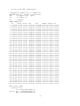
Table 1: Numerical experiments(SDPA 7.0.5 + BLAS library) : time:sec.(# of iterations)
BLAS library(# of threads)
BLAS/LAPACK 3.1.1(1)
ATLAS 3.8.1(1)
ATLAS 3.8.1(4)
Intel MKL 10.0.2.018(1)
Intel MKL 10.0.2.018(2)
Intel MKL 10.0.2.018(4)
Intel MKL 10.0.2.018(8)
GotoBLAS 1.24(1)
GotoBLAS 1.24(2)
GotoBLAS 1.24(4)
GotoBLAS 1.24(8)
Prob(1)
70.51(36)
53.00(35)
32.76(35)
44.25(35)
32.88(35)
26.61(35)
25.17(35)
42.94(34)
31.81(35)
26.60(36)
23.84(35)
Prob(2)
128.36(15)
49.86(15)
19.66(15)
39.92(15)
24.43(15)
16.38(15)
13.38(15)
40.37(15)
23.89(15)
14.81(15)
11.57(15)
Prob(3)
226.24(18)
41.24(18)
18.26(18)
34.63(18)
22.44(18)
16.37(18)
14.83(18)
32.42(18)
21.07(18)
15.59(18)
13.95(18)
Prob(4)
342.42(20)
182.65(19)
81.73(19)
172.05(21)
110.41(22)
67.78(18)
63.01(19)
160.75(21)
99.76(20)
64.29(18)
67.47(21)
CPU : Intel Xeon 5345 (2.33GHz) × 2 CPUs, 8 cores
OS : CentOS Ver 5.1 64bit
Compiler : Intel (C/C++ & Fortran) 10.1.012
Table 2: Numerical experiments(SDPA 7.0.5 + BLAS library) : time:sec.(# of iterations)
BLAS library(# of threads)
BLAS/LAPACK 3.1.1(1)
ATLAS 3.8.1(1)
ATLAS 3.8.1(2)
Intel MKL 10.0.2.018(1)
Intel MKL 10.0.2.018(2)
GotoBLAS 1.24(1)
GotoBLAS 1.24(2)
Prob(1)
49.48(36)
40.29(35)
29.76(35)
33.39(35)
25.00(35)
33.91(36)
24.52(35)
Prob(2)
67.23(15)
37.27(15)
23.22(15)
30.49(15)
18.72(15)
40.23(15)
18.37(15)
CPU : Intel Core 2 E8200 (2.66GHz) × 1 CPU, 2 cores
OS : CentOS Ver 5.1 64bit
Compiler : Intel (C/C++ & Fortran) 10.1.012
Prob(1)
Prob(2)
Prob(3)
Prob(4)
:
:
:
:
Structural Optimization : g1717.dat-s
Combinatorial Optimization(1) : mcp1000-10.dat-s
Combinatorial Optimization(2) : theta5.dat-s
Quantum Chemistry : CH.2Pi.STO6G.pqg.dat-s
6
Prob(3)
143.84(18)
32.14(18)
21.12(18)
26.68(18)
17.56(18)
24.53(18)
16.11(18)
Prob(4)
220.38(20)
145.72(20)
99.04(21)
129.72(21)
84.24(22)
109.72(19)
71.53(19)
Supply a command line to link against your BLAS, e.g.,
--with-blas="-L/home/nakata/gotoblas/lib -lgoto" .
• --with-lapack
Supply a command line to link against your LAPACK, e.g.,
--with-lapack="-L/home/nakata/gotoblas/lib -lgoto -llapack" .
1.6.2
Linking Against ATLAS
Install ATLAS, and assume that the ATLAS libraries are installed at “/home/nakata/atlas/lib”.
If there exists “liblapack.a” at ‘/home/nakata/atlas/lib”, we recommend rename or remove it. Then,
reconfigure and rebuild the SDPA like following.
$ make clean
$ ./configure --with-blas="-L/home/nakata/atlas/lib -lptf77blas -lptcblas -latlas"
$ make
The number of cores uses is determined at the build process, and you need a multi-core CPU to accelerate
BLAS operations.
1.6.3
Linking Against GotoBLAS
Install GotoBLAS, and assume that the GotoBLAS libraries are installed at “/home/nakata/gotoblas/lib”.
Reconfigure and rebuild the SDPA like following.
$ make clean
$ ./configure --with-blas="-L/home/nakata/gotoblas/lib -lgoto" \
--with-lapack="-L/home/nakata/gotoblas/lib -lgoto -llapack"
$ make
You can set the number of threads uses via setting the “OMP NUM THREADS” environment variable
before running the SDPA like following. In this case, two cores will be used for BLAS operations. You need
a multi-core CPU to accelerate BLAS operations.
$ export OMP_NUM_THREADS=2
$ sdpa -ds example1.dat-s -o example1.out
1.6.4
Linking Against Intel Math Kernel Library
Install Intel Math Kernel Library, and assume that the library is installed at “/opt/intel/mkl/10.0.3.020/lib/em64t”.
Reconfigure and rebuild the SDPA like following.
$ make clean
$ ./configure --with-blas="-L/opt/intel/mkl/10.0.3.020/lib/em64t -lmkl_em64t -lguide" \
--with-lapack="-L/opt/intel/mkl/10.0.3.020/lib/em64t -lmkl_lapack -lmkl_sequential -lmkl_core"
$ make
You can set the number of threads uses via setting the “OMP NUM THREADS” environment variable
before running the SDPA like following. In this case, four cores will be used for BLAS operations. You
need a multi-core CPU to accelerate BLAS operations.
$ export OMP_NUM_THREADS=4
$ sdpa -ds example1.dat-s -o example1.out
7
1.7
Performance Tuning: Compiler Options
We also recommend adding some optimized flags to the compilers. Our recommendations are
• -O2 -funroll-all-loops (default)
• -static -O3 -funroll-all-loops -march=nocona -msse3 -mfpmath=sse (on Core2).
The above default options are sufficient for better performance in many cases. To pass your optimization
flags, set them in CFLAGS and CXXFLAGS environment variables. Here is an example:
$
$
$
$
$
bash
make clean
export CFLAGS="-static -funroll-all-loops -O3 -m64 -march=nocona -msse3 -mfpmath=sse"
export CXXFLAGS="-static -funroll-all-loops -O3 -m64 -march=nocona -msse3 -mfpmath=sse"
./configure --with-blas="-L/home/nakata/gotoblas/lib -lgoto" \
--with-lapack="-L/home/nakata/gotoblas/lib -lgoto -llapack"
$ make
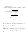
2.
Semidefinite Program
2.1
Standard Form SDP and Its Dual
The SDPA (Semidefinite Programming Algorithm) solves the following standard form semidefinite program
and its dual.
m
X
P: minimize
ci xi
i=1
m
X
SDP
subject
to
X
=
F i xi − F 0 , S 3 X º O,
i=1
D: maximize
F0 • Y
subject to F i • Y = ci (i = 1, 2, . . . , m), S 3 Y º O.
S : set of n × n real symmetric matrices
F i ∈ S (i = 0, 1, . . . , m) : constraint matrices
O ∈ S : zero matrix
c1
x1
c2
x2
c = . ∈ Rm : cost vector, x = .
..
..
cm
X ∈ S, Y ∈ S : variable matrices
∈ Rm : variable vector
xm
U • V : inner product between U and V ∈ S, i.e.,
n X
n
X
Uij Vij
i=1 j=1
U º O ⇐⇒ U ∈ S is positive semidefinite
Throughout this manual, we denote the primal SDP by P and its dual problem by D. The SDP is determined
by m, n, c ∈ Rm , and F i ∈ S (i = 0, 1, . . . , m). When (x, X) is a feasible solution (or a minimum solution,
resp.) of the primal problem P and Y is a feasible solution (or a maximum solution, resp.), we call (x, X, Y )
a feasible solution (or an optimal solution, resp.) of the SDP.
We assume:
8
Condition 1.1. {F i : i = 1, 2, . . . , m} ⊂ S is linearly independent.
If a given SDP does not satisfy this assumption, the SDPA can abnormally stop due to some numerical
instability, but it does not mean that it will necessarily happen.
If we deal with a different primal-dual pair P 0 and D0 of the form
P’ : minimize
A0 • X
subject to Ai • X = bi (i = 1, 2, . . . , m), S 3 X º O,
m
X
D’ : maximize
bi yi
SDP’
i=1
m
X
subject to
Ai yi + Z = A0 , S 3 Z º O,
i=1
we can easily transform it into the standard form SDP as follows:
³
−Ai (i = 0, . . . , m) −→ F i (i = 0, . . . , m)
−bi (i = 1, . . . , m)
X
y
Z
µ
2.2
−→
−→
−→
−→
ci (i = 1, . . . , m)
Y
x
X
´
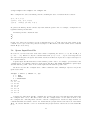
Example 1
P:
minimize
48y1 −
µ 8y2 + 20y
¶3
µ
µ
10 4
0
0
0
X=
y1 +
y2 +
4 0
0 −8
−8
X
µ º O.
−11 0
•Y
0 23
µ
µ
10 4
0
0
• Y = 48,
• Y = −8
0 −8
µ 4 0
0 −8
• Y = 20, Y º O.
−8 −2
subject to
D: maximize
subject to
Here
−8
−2
µ
y3 −
m
F1
µ
48
−11 0
= 3, n = 2, c = −8 , F 0 =
,
0 23
20
µ
µ
µ
10 4
0
0
0 −8
=
, F2 =
, F3 =
.
4 0
0 −8
−8 −2
The data of this problem is contained in the file “example1.dat” (see Section 4.1).
2.3
Example 2
m
= 5, n = 7, c =
1.1
−10
6.6
19
4.1
9
,
−11
0
0
23
F0
=
F1
=
−1.4 −3.2 0.0
0.0
0.0 0.0
0.0
−3.2 −28 0.0
0.0
0.0 0.0
0.0
0.0
0.0
15 −12
2.1 0.0
0.0
0.0
0.0 −12
16 −3.8 0.0
0.0
,
0.0
0.0 2.1 −3.8
15 0.0
0.0
0.0
0.0 0.0
0.0
0.0 1.8
0.0
0.0
0.0 0.0
0.0
0.0 0.0 −4.0
0.5
5.2
0.0
0.0 0.0
0.0
0.0
5.2 −5.3
0.0
0.0 0.0
0.0
0.0
0.0
0.0
7.8 −2.4 6.0
0.0
0.0
0.0
0.0 −2.4
4.2 6.5
0.0
0.0
,
0.0
0.0
6.0
6.5 2.1
0.0
0.0
0.0
0.0
0.0
0.0 0.0 −4.5
0.0
0.0
0.0
0.0
0.0 0.0
0.0 −3.5
•
•
•
F5
=
−6.5 −5.4
−5.4 −6.6
0.0
0.0
0.0
0.0
0.0
0.0
0.0
0.0
0.0
0.0
0.0
0.0
6.7
−7.2
−3.6
0.0
0.0
0.0
0.0
−7.2
7.3
−3.0
0.0
0.0
0.0
0.0
−3.6
−3.0
−1.4
0.0
0.0
0.0
0.0
0.0
0.0
0.0
6.1
0.0
0.0
0.0
0.0
0.0
0.0
0.0
−1.5
.
As shown in this example, the SDPA handles block diagonal matrices. The data of this example is contained
in the file “example2.dat” (see Section 4.2).
3.
Files Necessary to Execute the SDPA
We need the following files to execute the SDPA:
• “sdpa” — The executable binary for solving an SDP.
• “input data file” — Any file name with the postfix “.dat” or “.dat-s” are accepted; for example,
“problem.dat” and “example.dat-s” are legitimate names for input files. The SDPA distinguishes a
dense input data file with the postfix “.dat” from a sparse input data file with the postfix “.dat-s”.
See Sections 4. and 7.2 for details.
• “param.sdpa” — The file describing the parameters used in the “sdpa”. See Section 5. for details.
The name is fixed to “param.sdpa”.
• “output file” — Any file name excepting “sdpa” and “param.sdpa”. For example, “problem.1” and
“example.out” are legitimate names for output files. See Section 6. for more details.
The files “example1.dat” (see Section 4.1) and “example2.dat” (see Section 4.2) contain the input date
of Example 1 and Example 2, respectively, which we have stated in the previous section. To solve Example 1,
type
$ ./sdpa example1.dat example1.out
Here “example1.out” denotes an “output file” in which the SDPA stores computational results such as an
approximate optimal solution, an approximate optimal value of Example 1, etc. Similarly, we can solve
Example 2.
10
4.
Input Data File
4.1
“example1.dat” — Input Data File of Example 1
"Example 1: mDim = 3,
3 = mDIM
1 = nBLOCK
2 = bLOCKsTRUCT
{48, -8, 20}
{ {-11, 0}, { 0, 23}
{ { 10, 4}, { 4, 0}
{ { 0, 0}, { 0, -8}
{ { 0, -8}, {-8, -2}
4.2
nBLOCK = 1, {2}"
}
}
}
}
“example2.dat” — Input Data File of Example 2
*Example 2:
*mDim = 5, nBLOCK = 3, {2,3,-2}
5 = mDIM
3 = nBLOCK
(2, 3, -2)
= bLOCKsTRUCT
{1.1, -10, 6.6, 19, 4.1}
{
{ { -1.4, -3.2 },
{ -3.2,-28
} }
{ { 15, -12,
2.1 },
{-12,
16,
-3.8 },
{ 2.1, -3.8, 15
}
}
{ 1.8, -4.0 }
}
{
{ { 0.5, 5.2 },
{ 5.2, -5.3 }
}
{ { 7.8, -2.4, 6.0 },
{ -2.4, 4.2, 6.5 },
{ 6.0, 6.5, 2.1 }
}
{ -4.5, -3.5 }
}
•
•
•
{
{ {
{
{ {
{
{
{
}
-6.5,
-5.4,
6.7,
-7.2,
-3.6,
6.1,
-5.4 },
-6.6 }
}
-7.2, -3.6 },
7.3, -3.0 },
-3.0, -1.4 }
-1.5 }
}
11
4.3
Format of the Input Data File
In general, the structure of an input data file is as follows:
Title and Comments
m — number of the primal variables xi ’s
nBLOCK — number of blocks
bLOCKsTRUCT — block structure vector
c
F0
F1
..
.
Fm
In Sections 4.4 through 4.8, we explain each item of the input data file in details.
4.4
Title and Comments
On the top of the input data file, we can write a single or multiple lines for “Title and Comments”. Each
line of “Title and Comments” must begin with " or * and should consist of no more than 75 letters; for
example
"Example 1: mDim = 3, nBLOCK = 1, {2}"
in the file “example1.dat”, and
*Example 2:
*mDim = 5, nBLOCK = 3, {2,3,-2}
in the file “example2.dat”. The SDPA displays “Title and Comments” when it starts. “Title and Comments”
can be omitted.
4.5
Number of the Primal Variables
We write the number m of the primal variables in a line following the line(s) of “Title and Comments” in
the input data file. All the letters after m through the end of the line are neglected. We have
3
=
mDIM
in the file “example1.dat”, and
5
=
mDIM
in the file “example2.dat”. In either case, the letters “= mDIM” are neglected.
12
4.6
Number of Blocks and the Block Structure Vector
The SDPA handles block diagonal matrices as we have seen in Section 2.3. We express a common matrix
data structure for the constraint matrices F 0 , F 1 , . . . , F m using the terms number of blocks, denoted by
nBLOCK, and block structure vector, denoted by bLOCKsTRUCT. If we deal with a block diagonal matrix
F of the form
B1
O O ··· O
O B2 O · · · O
F
=
,
..
..
.. . .
(1)
. O
.
.
.
O
O O · · · B`
Bi :
a pi × pi symmetric matrix (i = 1, 2, . . . , `),
we define the number nBLOCK of blocks and the block structure vector bLOCKsTRCTURE as follows:
nBLOCK
bLOCKsTRUCT
=
=
βi
=
For example, if F is of the form
1
2
3
0
0
0
0
`,
(β1 , β2 , . . . , β` ),
½
pi if B i is a symmetric matrix,
−pi if B i is a diagonal matrix.
2
4
5
0
0
0
0
3
5
6
0
0
0
0
0
0
0
1
2
0
0
0
0
0
2
3
0
0
0
0
0
0
0
4
0
0
0
0
0
0
0
5
,
(2)
we have
nBLOCK = 3
If
?
F = ?
?
?
?
?
and
bLOCKsTRUCT =
(3, 2, −2)
?
? , where ? denotes a real number,
?
is a usual symmetric matrix with no block diagonal structure, we define
nBLOCK = 1 and bLOCKsTRUCT = 3
We separately write each of nBLOCK and bLOCKsTRUCT in one line. Any letter after either of nBLOCK
and bLOCKsTRUCT through the end of the line is neglected. In addition to blank letter(s), and the tab
code(s), we can use the letters
,
( ) { }
to separate elements of the block structure vector bLOCKsTRUCT. We have
1
2
= nBLOCK
= bLOCKsTRUCT
in Example 1 (see the file “example1.dat” in Section 4.1), and
3
2
=
nBLOCK
-2
3
= bLOCKsTRUCT
in Example 2 (see the file “example2.dat” in Section 4.2). In either case, the letters “= nBLOCK” and “=
bLOCKsTRUCT” are neglected.
13
4.7
Constant Vector
Specify all the elements c1 , c2 , . . ., cm of the cost vector c. In addition to blank letter(s) and tab code(s),
we can use the letters
,
( ) { }
to separate elements of the vector c. We have
{48, -8, 20}
in Example 1 (see the file “example1.dat” in Section 4.1), and
{1.1, -10, 6.6, 19, 4.1}
in Example 2 (see the file “example2.dat” in Section 4.2).
4.8
Constraint Matrices
We describe the constraint matrices F 0 , F 1 , . . . , F m according to the data format specified by nBLOCK
and bLOCKsTRUCT stated in Section 4.6. In addition to blank letter(s) and tab code(s), we can use the
letters
,
( ) { }
to separate elements of the matrices F 0 , F 1 , . . . , F m and their elements. In the general case of the
block diagonal matrix F given in (1), we write the elements of B 1 , B 2 , . . . B ` sequentially; when B i is a
diagonal matrix, we write only the diagonal elements sequentially. For instance, for the matrix F given by
(2) (nBLOCK = 3, bLOCKsTRUCT = (3, 2, −2)), the corresponding representation of the matrix F turns
out to be
{ {{1
2
3} {2
4
5} {3
5
6}}, {{1
2} {2
3}}, {4, 5} }
In Example 1 with nBLOCK = 1 and bLOCKsTRUCT = 2, we have
{
{
{
{
{-11, 0},
{ 10, 4},
{ 0, 0},
{ 0, -8},
{ 0, 23} }
{ 4, 0} }
{ 0, -8} }
{-8, -2} }
See the file “example1.dat” in Section 4.1.
In Example 2 with nBLOCK = 3 and bLOCKsTRUCT = (2, 3, −2), we have
{
{ { -1.4, -3.2 },
{ -3.2,-28
}
}
{ { 15, -12,
2.1
{-12,
16,
-3.8
{ 2.1, -3.8, 15
{ 1.8, -4.0 }
}
{
{ { 0.5, 5.2 },
{ 5.2, -5.3 }
}
{ { 7.8, -2.4, 6.0
{ -2.4, 4.2, 6.5
{ 6.0, 6.5, 2.1
{ -4.5, -3.5 }
}
},
},
}
}
},
},
}
}
14
•
•
•
{
{ {
{
{ {
{
{
{
}
-6.5,
-5.4,
6.7,
-7.2,
-3.6,
6.1,
-5.4 },
-6.6 }
}
-7.2, -3.6 },
7.3, -3.0 },
-3.0, -1.4 }
-1.5 }
}
See the file “example2.dat” in Section 4.2.
Remark. We can also write the input data of Example 1 without using any letters
,
(
)
{
}
such as
"Example 1: mDim = 3, nBLOCK = 1, {2}"
3
1
2
48 -8 20
-11
0
0 23
10
4
4
0
0
0
0 -8
0 -8 -8 -2
5.
Parameter File
First we show the default parameter file “param.sdpa” below.
40
1.0E-7
1.0E2
2.0
-1.0E5
1.0E5
0.1
0.2
0.9
1.0E-7
unsigned int maxIteration;
double 0.0 < epsilonStar;
double 0.0 < lambdaStar;
double 1.0 < omegaStar;
double lowerBound;
double upperBound;
double 0.0 <= betaStar < 1.0;
double 0.0 <= betaBar < 1.0, betaStar <= betaBar;
double 0.0 < gammaStar < 1.0;
double 0.0 < epsilonDash;
The file “param.sdpa” needs to have these 10 lines which sets 10 parameters. Each line of this file contains
one of the 10 parameters followed by an comment. When the SDPA reads the file “param.sdpa”, it neglects
the comments.
• maxIteration — Maximum number of iterations. The SDPA stops when the iteration exceeds maxIteration.
15
• epsilonStar, epsilonDash — The accuracy of an approximate optimal solution of the SDP. When the
current iterate (xk , X k , Y k ) satisfies all of the inequalities
¯
(¯
)
m
¯
¯
¯ k X
¯
k
epsilonDash ≥ max ¯[X −
F i xi + F 0 ]pq ¯ : p, q = 1, 2, . . . , n ,
¯
¯
i=1
¯
n¯
o
¯
¯
epsilonDash ≥ max ¯F i • Y k − ci ¯ : i = 1, 2, . . . , m ,
Pm
| i=1 ci xki − F 0 • Y k |
n
o
epsilonStar ≥
Pm
max (| i=1 ci xki | + |F 0 • Y k |)/2.0, 1.0
=
|primal objective value − dual objective value|
,
max{(|primal objective value| + |dual objective value|)/2.0, 1.0}
the SDPA stops. Too small epsilonStar and epsilonDash may cause numerical instability. A reasonable
choice is epsilonStar and epsilonDash ≥ 1.0E − 7.
• lambdaStar — This parameter determines an initial point (x0 , X 0 , Y 0 ) such that
x0 = 0, X 0 = lambdaStar × I, Y 0 = lambdaStar × I.
Here I denotes the identity matrix. It is desirable to choose an initial point (x0 , X 0 , Y 0 ) having the
same order of magnitude of an optimal solution (x∗ , X ∗ , Y ∗ ) of the SDP. In general, however, choosing
such lambdaStar is difficult. If there is no information on the magnitude of an optimal solution
(x∗ , X ∗ , Y ∗ ) of the SDP, we strongly recommend to take a sufficiently large lambdaStar such that
X ∗ ¹ lambdaStar × I
and
Y ∗ ¹ lambdaStar × I.
• omegaStar — This parameter determines the region in which the SDPA searches an optimal solution.
For the primal problem P, the SDPA searches a minimum solution (x, X) within the region
O ¹ X ¹ omegaStar × X 0 = omegaStar × lambdaStar × I,
and stops the iteration if it detects that the primal problem P has no minimum solution in this region.
For the dual problem D, the SDPA searches a maximum solution Y within the region
O ¹ Y ¹ omegaStar × Y 0 = omegaStar × lambdaStar × I,
and stops the iteration if it detects that the dual problem D has no maximum solution in this region.
Again we recommend to take a large lambdaStar and a small omegaStar > 1.
• lowerBound — Lower bound of the minimum objective value of the primal problem P. When the
m
X
SDPA generates a primal feasible solution (xk , X k ) whose objective value
ci xki gets smaller than
i=1
the lowerBound, the SDPA stops the iteration; the primal problem P is likely to be unbounded and
the dual problem D is likely to be infeasible if the lowerBound is sufficiently small.
• upperBound — Upper bound of the maximum objective value of the dual problem D. When the
SDPA generates a dual feasible solution Y k whose objective value F 0 • Y k gets larger than the
upperBound, the SDPA stops the iteration; the dual problem D is likely to be unbounded and the
primal problem P is likely to be infeasible if the upperBound is sufficiently large.
• betaStar — Parameter controlling the search direction when (xk , X k , Y k ) is feasible. As we take a
smaller betaStar > 0.0, the search direction tends to get closer to the affine scaling direction without
centering.
• betaBar — Parameter controlling the search direction when (xk , X k , Y k ) is infeasible. As we take a
smaller betaBar > 0.0, the search direction tends to get closer to the affine scaling direction without
centering. The value of betaBar must be no less than the value of betaStar; 0 ≤ betaStar ≤ betaBar.
• gammaStar — Reduction factor for the primal and dual step lengths; 0.0 < gammaStar < 1.0.
16
6.
Output
6.1
Execution of the SDPA
To execute the SDPA, we specify and type the names of three files, “sdpa”, an “input data file” and an
“output file” as follows.
$ sdpa
"input data file"
"output file"
To solve Example 1, type:
$ sdpa example1.dat example1.out
6.2
Output on the Display
The SDPA shows some information on the display. In the case of Example 1, we have
SDPA start at
Fri Dec 7 18:30:56 2007
data
is example1.dat-s : sparse
parameter is ./param.sdpa
out
is example.1.out
DENSE computations
mu
thetaP
0 1.0e+04 1.0e+00
1 1.6e+03 0.0e+00
2 1.7e+02 2.3e-16
3 1.8e+01 2.3e-16
4 1.9e+00 2.6e-16
5 1.9e-01 2.6e-16
6 1.9e-02 2.5e-16
7 1.9e-03 2.6e-16
8 1.9e-04 2.5e-16
9 1.9e-05 2.7e-16
10 1.9e-06 2.6e-16
thetaD
1.0e+00
9.4e-02
3.6e-03
1.5e-17
1.5e-17
3.0e-17
1.6e-15
2.2e-17
1.5e-17
7.5e-18
5.0e-16
objP
-0.00e+00
+8.39e+02
+1.96e+02
-6.84e+00
-3.81e+01
-4.15e+01
-4.19e+01
-4.19e+01
-4.19e+01
-4.19e+01
-4.19e+01
objD
+1.20e+03
+7.51e+01
-3.74e+01
-4.19e+01
-4.19e+01
-4.19e+01
-4.19e+01
-4.19e+01
-4.19e+01
-4.19e+01
-4.19e+01
phase.value = pdOPT
Iteration = 10
mu = 1.9180668442024010e-06
relative gap = 9.1554505577840628e-08
gap = 3.8361336884048019e-06
digits = 7.0383202783481345e+00
objValPrimal = -4.1899996163866390e+01
objValDual
= -4.1899999999999999e+01
p.feas.error = 3.2137639581876834e-14
d.feas.error = 4.7961634663806763e-13
total time
= 0.010
main loop time = 0.010000
total time = 0.010000
file
read time = 0.000000
file
read time = 0.000000
17
alphaP
1.0e+00
2.3e+00
1.3e+00
9.9e-01
1.0e-00
1.0e-00
1.0e-00
1.0e-00
1.0e-00
1.0e-00
1.0e-00
alphaD
9.1e-01
9.6e-01
1.0e+00
9.9e-01
1.0e-00
9.0e+01
1.0e-00
1.0e-00
1.0e-00
9.0e+01
9.0e+01
beta
2.00e-01
2.00e-01
2.00e-01
1.00e-01
1.00e-01
1.00e-01
1.00e-01
1.00e-01
1.00e-01
1.00e-01
1.00e-01
• mu — The average complementarity X k • Y k /n (optimality measure). When both P and D get
feasible, the relation
Ãm
!
X
k
k
mu =
ci xi − F 0 • Y
/n
i=1
=
primal objective function - dual objective function
n
holds.
• thetaP — The SDPA starts with thetaP = 0.0 if the initial point (x0 , X 0 ) of the primal problem P
is feasible, and thetaP = 1.0 otherwise; hence it usually starts with thetaP = 1.0. In the latter case,
the thetaP at the kth iteration is given by
¯
o
n¯
Pm
¯
¯
max ¯[X k − i=1 F i xki + F 0 ]p,q ¯ : p, q = 1, 2, . . . , n
¯
©¯
ª;
thetaP =
Pm
max ¯[X 0 − i=1 F i x0i + F 0 ]p,q ¯ : p, q = 1, 2, . . . , n
The thetaP is theoretically monotone non-increasing, and when it gets 0.0, we obtain a primal feasible
solution (xk , X k ). In the example above, we obtained a primal feasible solution in the 1st iteration.
• thetaD — The SDPA starts with thetaD = 0.0 if the initial point Y 0 of the dual problem D is feasible,
and thetaD = 1.0 otherwise; hence it usually starts with thetaD = 1.0. In the latter case, the thetaD
at the kth iteration is given by
¯
n¯
o
¯
¯
max ¯F i • Y k − ci ¯ : i = 1, 2, . . . , m
¯
©¯
ª;
thetaD =
max ¯F i • Y 0 − ci ¯ : i = 1, 2, . . . , m
The thetaD is theoretically monotone non-increasing, and when it gets 0.0, we obtain a dual feasible
solution Y k . In the example above, we obtained a dual feasible solution in the 3rd iteration.
• objP — The primal objective function value.
• objD — The dual objective function value.
• alphaP — The primal step length.
• alphaD — The dual step length.
• beta — The search direction parameter.
• phase.value — The status when the iteration stops, taking one of the values pdOPT, noINFO, pFEAS,
dFEAS, pdFEAS, pdINF, pFEAS dINF, pINF dFEAS, pUNBD and dUNBD.
pdOPT : The normal termination yielding both primal and dual approximate optimal solutions.
noINFO : The iteration has exceeded the maxIteration and stopped with no information on the
primal feasibility and the dual feasibility.
pFEAS : The primal problem P got feasible but the iteration has exceeded the maxIteration and
stopped.
dFEAS : The dual problem D got feasible but the iteration has exceeded the maxIteration and
stopped.
pdFEAS : Both primal problem P and the dual problem D got feasible, but the iteration has
exceeded the maxIteration and stopped.
pdINF : At least one of the primal problem P and the dual problem D is expected to be infeasible.
More precisely, there is no optimal solution (x, X, Y ) of the SDP such that
O ¹ X ¹ omegaStar × X 0 ,
O ¹ Y ¹ omegaStar × Y 0 ,
m
X
ci xi = F 0 • Y .
i=1
18
pFEAS dINF : The primal problem P has become feasible but the dual problem is expected to be
infeasible. More precisely, there is no dual feasible solution Y such that
O ¹ Y ¹ omegaStar × Y 0 = lambdaStar × omegaStar × I.
pINF dFEAS : The dual problem D has become feasible but the primal problem is expected to be
infeasible. More precisely, there is no feasible solution (x, X) such that
O ¹ X ¹ omegaStar × X 0 = lambdaStar × omegaStar × I.
pUNBD : The primal problem is expected to be unbounded. More precisely, the SDPA has stopped
generating a primal feasible solution (xk , X k ) such that
objP =
m
X
ci xki < lowerBound.
i=1
dUNBD : The dual problem is expected to be unbounded. More precisely, the SDPA has stopped
generating a dual feasible solution Y k such that
objD = F 0 • Y k > upperBound.
• Iteration — The iteration number when the SDPA terminated.
• relative gap — The relative gap
|objP − objD|
.
max {1.0, (|objP| + |objD|) /2}
This value is compared with epsilonStar (Section 5.).
• gap — The gap is mu × n.
• digits — This value indicates how objP and objD resemble by the following definition.
digits
=
− log10
=
− log10
|objP − objD|
(|objP| + |objD|)/2.0
Pm
| i=1 ci xi k − F 0 • Y k |
Pm
(| i=1 ci xi k | + |F 0 • Y k |)/2.0
• objValPrimal — The primal objective function value
objValPrimal =
m
X
ci xki .
i=1
• objValDual — The dual objective function value
objValD = F 0 • Y k .
• p.feas.error — This value indicates the primal infeasibily in the last iteration,
¯
(¯
)
m
¯
¯
¯ k X
¯
k
p.feas.error = max ¯[X −
F i xi + F 0 ]p,q ¯ : p, q = 1, 2, . . . , n
¯
¯
i=1
This value is compared with epsilonDash (Section 5.). Even if the primal problem is feasible, this
value may not be 0 due to numerical errors.
• d.feas.error — This value indicates the dual infeasibily in the last iteration,
¯
n¯
o
¯
¯
d.feas.error = max ¯F i • Y k − ci ¯ : i = 1, 2, . . . , m .
This value is compared with epsilonDash (Section 5.). Even if the dual problem is feasible, this
value may not be 0 due to numerical errors.
19
• total time — This value indicates how much time the SDPA needs to execute all subroutines.
• main loop time —This value indicates how much time the SDPA needs between the first iteration
and the last iteration.
• file read time — This value is how much time the SDPA needs to read from the input file and store
the data in memory.
6.3
Output to a File
We show the content of the file “example2.out” on which the SDPA has written the computational results
of Example 2.
SDPA start at Fri Dec 7 18:32:10 2007
*Example 2:
*mDim = 5, nBLOCK = 3, {2,3,-2}
data
is example2.dat
parameter is ./param.sdpa
out
is example2.out
mu
thetaP thetaD objP
objD
0 1.0e+04 1.0e+00 1.0e+00 -0.00e+00 +1.44e+03
1 3.3e+03 1.2e-01 3.4e-01 +4.94e+02 +2.84e+02
2 9.0e+02 4.9e-16 6.2e-02 +8.66e+02 -2.60e+00
3 1.4e+02 4.9e-16 8.8e-17 +9.67e+02 +9.12e-01
4 1.8e+01 2.6e-16 8.6e-16 +1.46e+02 +2.36e+01
5 2.7e+00 3.3e-16 4.2e-16 +4.62e+01 +2.74e+01
6 5.7e-01 3.2e-16 2.0e-16 +3.43e+01 +3.03e+01
7 9.5e-02 3.3e-16 4.1e-17 +3.24e+01 +3.18e+01
8 1.3e-02 3.2e-16 1.9e-17 +3.21e+01 +3.20e+01
9 1.5e-03 3.5e-16 2.8e-17 +3.21e+01 +3.21e+01
10 1.5e-04 3.2e-16 1.7e-17 +3.21e+01 +3.21e+01
11 1.5e-05 3.4e-16 3.7e-17 +3.21e+01 +3.21e+01
12 1.5e-06 3.2e-16 4.3e-17 +3.21e+01 +3.21e+01
13 1.5e-07 3.3e-16 3.1e-17 +3.21e+01 +3.21e+01
phase.value = pdOPT
Iteration = 13
mu = 1.5017857203245200e-07
relative gap = 3.2787330975500860e-08
gap = 1.0512500042271640e-06
digits = 7.4842939352608049e+00
objValPrimal = 3.2062693405e+01
objValDual
= 3.2062692354e+01
p.feas.error = 3.7747582837e-14
d.feas.error = 5.8841820305e-14
total time
= 0.000
Parameters are
maxIteration =
epsilonStar =
lambdaStar
=
omegaStar
=
lowerBound
=
upperBound
=
betaStar
=
100
1.000e-07
1.000e+02
2.000e+00
-1.000e+05
1.000e+05
1.000e-01
20
alphaP
8.8e-01
1.0e+00
1.0e+00
9.5e-01
9.3e-01
8.1e-01
9.2e-01
9.5e-01
9.8e-01
9.9e-01
9.9e-01
9.9e-01
9.9e-01
9.9e-01
alphaD
6.6e-01
8.2e-01
1.0e+00
5.4e+00
1.5e+00
1.4e+00
9.3e-01
9.6e-01
1.0e-00
1.0e+00
1.0e+00
1.0e+00
1.0e+00
1.0e+00
beta
2.00e-01
2.00e-01
2.00e-01
1.00e-01
1.00e-01
1.00e-01
1.00e-01
1.00e-01
1.00e-01
1.00e-01
1.00e-01
1.00e-01
1.00e-01
1.00e-01
betaBar
gammaStar
epsilonDash
= 2.000e-01
= 9.000e-01
= 1.000e-07
Time(sec)
Predictor time =
0.000000,
... abbreviation ...
Total
=
0.000000,
Ratio(% : MainLoop)
nan
nan
xVec =
{+1.552e+00,+6.710e-01,+9.815e-01,+1.407e+00,+9.422e-01}
xMat =
{
{ {+6.392e-08,-9.638e-09 },
{-9.638e-09,+4.539e-08 }
}
{ {+7.119e+00,+5.025e+00,+1.916e+00 },
{+5.025e+00,+4.415e+00,+2.506e+00 },
{+1.916e+00,+2.506e+00,+2.048e+00 }
}
{+3.432e-01,+4.391e+00}
}
yMat =
{
{ {+2.640e+00,+5.606e-01 },
{+5.606e-01,+3.718e+00 }
}
{ {+7.616e-01,-1.514e+00,+1.139e+00 },
{-1.514e+00,+3.008e+00,-2.264e+00 },
{+1.139e+00,-2.264e+00,+1.705e+00 }
}
{+4.087e-07,+3.195e-08}
}
main loop time = 0.000000
total time = 0.000000
file
read time = 0.000000
Now we explain the items that appeared above in the file “example2.out”.
• Lines with start ‘*’ — These lines are comments in “example2.dat”.
• Data, parameter, initial, output — These are the file names we assigned for data, parameter, initial
point, and output, respectively.
• Lines between “Predictor time” to “Total time” — These lines display the profile data. These
information may help us to tune up the parameters, but the details are rather complicate, because
the profile data seriously depends on internal algorithms.
• xVec — Approximate optimal primal variable vector x.
• xMat — Approximate optimal primal variable matrix X.
• yMat — Approximate optimal dual variable matrix Y .
6.4
Printing DIMACS Errors
To display the error measures defined at the 7th DIMACS Implementation Challenge on Semidefinite and
Related Optimization Problems [6],
1. Go to the subdirectory where SDPA source code is.
2. Edit the file sdpa io.cpp, line 22
21
#define DIMACS_PRINT 0
to
#define DIMACS_PRINT 1
3. Type “make clean”.
4. Type “make” to re-compile SDPA.
The SDPA will output on the display and in the output file the following DIMACS errors at the last
iteration:
• Err1 — The relative dual feasibility error on the constraints
qP
m
k
2
i=1 (F i • Y − ci )
1 + max{|ci | : i = 1, 2, . . . , m}
• Err2 — The relative dual feasibility error on the semidefiniteness
(
)
−λmin (Y k )
max 0,
1 + max{|ci | : i = 1, 2, . . . , m}
• Err3 — The relative primal feasibility error on the constraints
Pm
kX k − i=1 F i xki + F 0 kf
}
1 + max{|[F 0 ]ij | : i, j = 1, 2, . . . , n}
• Err4 — The relative primal feasibility error on the semidefiniteness
(
)
−λmin (X k )
max 0,
1 + max{|[F 0 ]ij | : i, j = 1, 2, . . . , n}
• Err5 — The relative duality gap 1
Pm
1+|
i=1
P
m
ci xki − F 0 • Y k
k
i=1 ci xi |
+ |F 0 • Y k |
• Err6 — The relative duality gap 2
1+|
Xk • Y k
k
k
i=1 ci xi | + |F 0 • Y |
Pm
where k · kf is a norm defined as a sum of the Frobenius norm of each block diagonal matrix, and λmin (·)
is the smallest eigenvalue of a matrix.
7.
Advanced Use of the SDPA
7.1
Initial Point
If a feasible interior solution (x0 , X 0 , Y 0 ) is known in advance, we may want to start the SDPA from
(x0 , X 0 , Y 0 ). In such a case, we can optionally specify a file which contains the data of a feasible interior
solution when we execute the SDPA; for example if we want to solve Example 1 from a feasible interior
initial point
µ
¶ µ
0.0
11.0 0.0
5.9 −1.375
(x0 , X 0 , Y 0 ) = −4.0 ,
,
,
1.0
0.0 9.0
−1.375
0.0
type
22
$ sdpa example1.dat example1.out example1.ini
Here “example1.ini” denotes an initial point file containing the data of a feasible interior solution:
{0.0, -4.0, 0.0}
{ {11.0, 0.0}, {0.0, 9.0} }
{ {5.9, -1.375}, {-1.375, 1.0} }
In general, the initial point file can have any name with the postfix “.ini”; for example, “example.ini” is a
legitimate initial point file name.
An initial point file contains the data
0
x
X0
Y0
in this order, where the description for the m-dimensional vector x0 must follow the same format as the
constant vector c (see Section 4.7), and the description of X 0 and Y 0 , the same format as the constraint
matrix F i (see Section 4.8).
7.2
Sparse Input Data File
In Section 4., we have stated the dense data format for inputting the data m, n, c ∈ Rm and F i ∈ S
(i = 0, 1, . . . , m). When not only the constant matrices F i ∈ S (i = 0, 1, . . . , m) are block diagonal, but
also each block is sparse, the sparse data format described in this section gives us a compact description of
the constant matrices.
A sparse input data file must have a name with the postfix “.dat-s”; for example, “problem.dat-s” and
“example.dat-s” are legitimate names for sparse input data files. The SDPA distinguishes a sparse input
data file with the postfix “.dat-s” from a dense input data file with the postfix “.dat”.
We show below the file “example1.dat-s”, which contains the data of Example 1 (Section 2.2) in the
sparse data format.
"Example 1: mDim = 3, nBLOCK = 1, {2}"
3 = mDIM
1 = nBLOCK
2 = bLOCKsTRUCT
48 -8 20
0 1 1 1 -11
0 1 2 2 23
1 1 1 1 10
1 1 1 2 4
2 1 2 2 -8
3 1 1 2 -8
3 1 2 2 -2
Compare the dense input data file “example1.dat” described in Section 4.1 with the sparse input data
file “example1.dat-s” above. The first 5 lines of the file “example1.dat-s” are the same as those of the
file “example1.dat”. Following them, each line of the file “example1.dat-s” describes a single element of a
constant matrix F i ; the 6th line “0 1 1 1 -11” means that the (1, 1)th element of the 1st block of the matrix
F 0 is −11, and the 11th line “3 1 1 2 -8” means that the (1, 2)th element of the 1st block of the matrix F 3
is −8.
23
In general, the structure of a sparse input data file is as follows:
Title and Comments
m — the number of the primal variables xi ’s
nBLOCK — the number of blocks
bLOCKsTRUCT — the block structure vector
c
k1 b1 i1 j1 v1
k2 b2 i2 j2 v2
...
kp bp ip jp vp
...
kq bq iq jq vq
Here kp ∈ {0, 1, . . . , m}, bp ∈ {1, 2, . . . , nBLOCK}, 1 ≤ ip ≤ jp and vp ∈ R. Each line “kp , bp , ip , jp , vp ”
means that the value of the (ip , jp )th element of the bp th block of the constant matrix F kp is vp . If the bp th
block is an ` × ` symmetric (non-diagonal) matrix then (ip , jp ) must satisfy 1 ≤ ip ≤ jp ≤ `; hence only
nonzero elements in the upper triangular part of the bp th block are described in the file. If the bp th block
is an ` × ` diagonal matrix then (ip , jp ) must satisfy 1 ≤ ip = jp ≤ `.
7.3
Sparse Initial Point File
We show below the file “example1.ini-s”, which contains an initial point data of Example 1 in the sparse
data format.
0.0
1 1
1 1
2 1
2 1
2 1
-4.0 0.0
1 1 11
2 2 9
1 1 5.9
1 2 -1.375
2 2 1
Compare the dense initial point file “example1.ini” described in Section 7.1 with the sparse initial file
“example1.ini-s” above. The first line of the file “example1.ini-s” is the same as that of the file “example1.ini”, which describes x0 in the dense format. Each line of the rest of the file “example1.ini-s” describes
a single element of an initial matrix X 0 if the first number of the line is 1, or a single element of an initial
matrix Y 0 if the first number of the line is 2; The 2nd line “1 1 1 1 11” means that the (1, 1)th element of
the 1st block of the matrix X 0 is 11, the 5th line “2 1 1 2 -1.375” means that the (1, 2)th element of the
1st block of the matrix Y 0 is −1.375.
A sparse initial point file must have a name with the postfix “.ini-s”; for example, “problem.ini-s” and
“example.ini-s” are legitimate names for sparse input data files. The SDPA distinguishes a sparse input
data file with the postfix “.ini” from a dense input data file with the postfix “.ini-s”
In general, the structure of a sparse input data file is as follows:
0
x
s1 b1 i1 j1 v1
s2 b2 i2 j2 v2
...
sp bp ip jp vp
...
sq bq iq , jq vq
Here sp = 1 or 2, bp ∈ {1, 2, . . . , nBLOCK}, 1 ≤ ip ≤ jp and vp ∈ R. When sp = 1, each line
“sp bp ip jp vp ” means that the value of the (ip , jp )th element of the bp th block of the constant matrix X 0
24
is vp . When sp = 2, the line “sp bp ip jp vp ” means that the value of the (ip , jp )th element of the bp th block
of the constant matrix Y 0 is vp . If the bp th block is an ` × ` symmetric (non-diagonal) matrix then (ip , jp )
must satisfy 1 ≤ ip ≤ jp ≤ `; hence only nonzero elements in the upper triangular part of the bp th block are
described in the file. If the bp th block is an ` × ` diagonal matrix then (ip , jp ) must satisfy 1 ≤ ip = jp ≤ `.
7.4
Obtaining More Precision on the Approximate Solution
By default, each element of the approximate optimal solution (xk , X k , Y k ) saved in the output file (see
Section 6.3) has a coefficient with 4 digits in scientific notation.
It is possible to increase its precision.
1. Go to the subdirectory where SDPA source code is.
2. Edit the file sdpa struct.cpp, line 25
#define P_FORMAT "%8.3e"
to, for instance,
#define P_FORMAT "%8.5e"
3. Type “make clean”.
4. Type “make” to re-compile SDPA.
Now, each element of the approximate optimal solution will have a coefficient with 6 digits in scientific
notation.
7.5
More on Parameter File
We may encounter some numerical difficult during the execution of the SDPA with the default parameter
file “param.sdpa”, and/or we may want to solve many easy SDPs with similar data more quickly. In such
a case, we need to adjust some of the default parameters: betaStar, betaBar, and gammaStar. We present
below two sets of those parameters. The one is the set “Stable but Slow” for difficult SDPs, and the other
is the set “Unstable but Fast” for easy SDPs.
Stable but Slow
1.0E4
double 0.0 < lambdaStar;
0.10 double 0.0 <= betaStar < 1.0;
0.30 double 0.0 <= betaBar < 1.0, betaStar <= betaBar;
0.80 double 0.0 < gammaStar < 1.0;
Unstable but Fast
0.01 double 0.0 <= betaStar < 1.0;
0.02 double 0.0 <= betaBar < 1.0, betaStar <= betaBar;
0.95 double 0.0 < gammaStar < 1.0;
Besides these parameters, the value of the parameter lambdaStar, which determines an initial point
(x0 , X 0 , Y 0 ), affects the computational efficiency and the numerical stability. Usually a larger lambdaStar
is safe although the SDPA may consume few more iterations.
25
8.
Transformation to the Standard Form of SDP
SDP has many applications, but frequently problems are not described in the standard form of SDP. In this
section, we show some examples on how to transform to the standard form of SDP.
8.1
Inequality Constraints
First, we consider the case where inequality constraints are added to the primal standard form of SDP. For
example,
m
X
minimize
ci xi
i=1
m
X
subject to X =
F i xi − F 0 , X º O,
i=1
m
m
X
X
1
1
αi xi ≤ β ,
αi2 xi ≥ β 2 .
i=1
Here,
αi1 , αi2
1
i=1
(i = 1, . . . , m), β , β ∈ R. In this case, we add slack variables (t1 , t2 ).
m
X
minimize
2
ci xi
i=1
subject to
X=
t1 =
m
X
F i xi − F 0 , X º O,
i=1
m
X
(−αi1 )xi − (−β 1 ),
i=1
t2 =
m
X
αi2 xi − β 2 ,
(t1 , t2 ) ≥ 0.
i=1
Hence we can reduce the above problem to the following standard form SDP.
m
X
minimize
ci xi
i=1
subject to
X̄ =
m
X
F̄ i xi − F̄ 0 , X̄ º O,
i=1
where
F̄ i =
Fi
−αi1
F0
,
F̄
=
0
αi2
, X̄ =
−β 1
β
X
,
t1
2
t2
nBlock = 2, blockStruct = (n, −2).
Next, we consider the case where
For example,
maximize
subject to
inequality constraints are added to the dual standard form of SDP.
F0 • Y
F 1 • Y = c1 , F 2 • Y = c2 ,
F 3 • Y ≤ c3 , F 4 • Y ≤ c4 , F 5 • Y ≥ c5 ,
Y º O.
In this case, we add slack variables (t3 , t4 , t5 ) to each inequality constraint.
maximize F 0 • Y
subject to F 1 • Y = c1 , F 2 • Y = c2 ,
F 3 • Y + t3 = c3 , F 4 • Y + t4 = c4 , F 5 • X − t5 = c5 ,
Y º O, (t3 , t4 , t5 ) ≥ 0.
26
Thus we can reduce the above problem to the following standard form SDP.
maximize F̄ 0 • Ȳ
subject to F̄ 1 • Ȳ = c1 , F̄ 2 • Ȳ = c2 ,
F̄ 3 • Ȳ = c3 , F̄ 4 • Ȳ = c4 , F̄ 5 • Ȳ = c5 ,
Ȳ º O,
where
Ȳ =
F̄ 2 =
F̄ 5 =
Y
, F̄ 0 =
t3
t4
t5
F2
0
0
0
0
F3
, F̄ 4 =
1
0
F1
,
0
0
0
F4
1
0
,
0
0
−1
nBlock = 2, blockStruct = (n, −3).
8.2
Norm Minimization Problem
Let Gi ∈ Rq×r (0 ≤ i ≤ p). The norm minimization problem is defined as:
°
°
p
°
°
X
°
°
minimize °G0 +
Gi xi °
°
°
i=1
subject to
xi ∈ R (1 ≤ i ≤ p).
Here kGk denotes the 2-norm of G, i.e.,
kGk = max kGuk = the square root of the maximum eigenvalue of GT G.
kuk=1
We can reduce this problem to an SDP:
minimize
xp+1
subject to
p µ
X
O
Gi
i=1
GTi
O
µ
xi +
I
O
O
I
µ
xp+1 +
O
G0
GT0
O
Thus if we take
m
Fi
F p+1
= p + 1,
µ
O
=
Gi
µ
I
=
O
µ
O
−GT0
n = r + q, F 0 =
,
−G0
O
GTi
, ci = 0 (1 ≤ i ≤ p),
O
O
, cp+1 = 1,
I
then we can reformulate the problem as the primal standard form of SDP.
27
,
0
0
F5
, F̄ 1 =
0
, F̄ 3 =
0
F0
º O.
8.3
Linear Matrix Inequality (LMI)
Let Gi ∈ S n (0 ≤ i ≤ p). We define the linear combinations of the matrices,
G(x) = G0 +
p
X
xi Gi ,
i=1
where x ∈ Rp . The Linear Matrix Inequality (LMI) [3] is defined as follows
G(x) º O.
We want to find x ∈ Rp which satisfies the LMI, or detect that any x ∈ Rp cannot satisfy the LMI.
Here we introduce an auxiliary variable xp+1 and convert the LMI into an SDP.
minimize
xp+1
subject to
X = G0 +
p
X
xi Gi − xp+1 I
º O, x ∈ Rp
i=1
We can reduce this LMI to the primal standard form of SDP if we take
m = p + 1, F 0 = −G0 , F i = Gi , ci = 0 (1 ≤ i ≤ p), F p+1 = −I, cp+1 = 1.
One important point of this SDP is that it always has a feasible solution. When we can get the optimal
solution with xp+1 ≥ 0, then (x1 , . . . , xp ) satisfies the LMI. On the other hand, if xp+1 < 0 then we can
conclude that the LMI cannot be satisfied by any x ∈ Rp .
8.4
SDP Relaxation of the Maximum Cut Problem
Let G = (V, E) be a complete undirected graph with a vertex set V = {1, 2, . . . , n} and an edge set
E = {(i, j) : i, j ∈ V, i < j}. We assign a weight Wij = Wji to each edge (i,
Pj) ∈ E. The maximum cut
problem is to find a partition (L, R) of V that maximizes the cut w(L, R) = i∈L,j∈R Wij . Introducing a
variable vector u ∈ Rn , we can formulate the problem as a nonconvex quadratic program:
n
maximize
n
1 XX
Wij (1 − ui uj ) subject to
4 i=1 j=1
u2i = 1 (1 ≤ i ≤ n).
Here each feasible solution u ∈ Rn of this problem corresponds to a cut (L, R) with L = {i ∈ V : ui = −1}
and R = {i ∈ V : ui = 1}. If we define W to be the n × n symmetric matrix with elements Wji = Wij
1
((i, j) ∈ E) and Wii = 0 (1 ≤ i ≤ n), and the n × n symmetric matrix C ∈ S n by C = (diag(W e) − W ),
4
where e ∈ Rn denotes the vector of ones and diag(W e) the diagonal matrix of the vector W e ∈ Rn , we
can rewrite the quadratic program above as
maximize
xT Cx subject to
x2i = 1 (1 ≤ i ≤ n).
If x ∈ Rn is a feasible solution of the latter quadratic program, then the n × n symmetric and positive
semidefinite matrix X whose (i, j)th element Xij is given by Xij = xi xj satisfies C • X = xT Cx and
Xii = 1 (1 ≤ i ≤ n). This leads to the following semidefinite programming relaxation of the maximum cut
problem:
maximize
C •X
(3)
subject to E ii • X = 1 (1 ≤ i ≤ n), X º O.
Here E ii denotes the n × n symmetric matrix with (i, i)th element 1 and all others 0.
28
8.5
Choosing Between the Primal and Dual Standard Forms
Any SDP can be formulated as a primal standard form P or as a dual standard form D (see Section 2.1). This
does not mean that one is the dual of the other, but simply that they are indeed two different formulations
of the same problem, each one having its dual counterpart.
Many times, it is advantageous to choose between the primal and the dual standard forms since one of
the formulations is more natural, has a smaller size, it is faster to solve, or it avoids numerical instability
on the software.
Let us consider as an example the SDP relaxation of the maximum cut problem (Section 8.4). We
formulated this SDP as a dual standard form D where the problem size is:
m = n
nBLOCK = 1
bLOCKsTRUCT = n.
We can also formulate (mathematically) the same problem as a primal standard form P, too.
Let H ij an n × n symmetric matrix with (i, j)th and (j, i)th element(s) 1 and all others 0. Problem (3)
is equivalent to
minimize
subject to
−2
n X
n
X
Cij xij −
i=1 j>i
n X
n
X
n
X
Cii xii
i=1
H ij xij º O,
(4)
i=1 j=i
xii ≥ 1 (1 ≤ i ≤ n),
xii ≤ 1 (1 ≤ i ≤ n),
where xij (1 ≤ i ≤ n, i ≤ j ≤ n) is a variable vector now.
This SDP is in primal standard form P and its size is
n(n + 1)
2
nBLOCK = 2
bLOCKsTRUCT = (n, −2n)
m
=
which seems less advantageous than the dual standard from D (3). Also the problem (4) in primal standard
form P does not have a strict feasible solution which many cause numerical instability.
In the case of n = 100, a typical running time for the formulation (3) in dual standard form is 0.18s,
while for the for the formulation (4) in primal standard form is 201.3s.
In some cases, however, a slight increase in the size of the problem can be advantageous if the new
formulation has more sparsity in its data.
9.
For the SDPA 6.2.1 Users
The major differences between the SDPA 6.2.1 and the SDPA 7.1.1 are the followings:
29
• The source code was completely revised, unnecessary variables were eliminated, and auxiliary variables
re-used. Consequently, the memory usage became less than half of the previous version.
• It utilizes the sparse Cholesky factorization when the Schur Complement Matrix becomes sparse. For
that, it uses the SPOOLES library for sparse matrices [2] to obtain an ordering of rows/columns
which possibly produces lesser fill-in. Now, the SDPA can solve much more efficiently SDPs with
– multiple block diagonal matrices
– multiple non-negative constraints
• There is a modification in the control subroutine in the interior-point algorithm which improved its
numerical stability when compared to the previous version.
Though it should be noted there is a remaining problem:
• The current version does not have a callable library interface as SDPA 6.2.1 does, but it will be
implemented in the updated version of the SDPA.
A
SDPA-GMP
The SDPA-GMP is an SDP solver intended to solve SDPs very accurately by utilizing the GNU Multiple
Precision Arithmetic Library (GMP). Current version of the SDPA-GMP is 7.1.1 which shares the same
features with the SDPA except for user settable accuracy usually for extraordinary accurate calculations.
Expect for newly added one parameters “precision”, user experience is the same as the SDPA. Note that
the SDPA-GMP is typically several ten or hundred times slower than the SDPA.
A1
Build and Installation
This subsection describes how to build and install the SDPA-GMP. Usually, the SDPA is distributed as
source codes, therefore, users must build it by themselves. We have build and installation tests on Fedora 8,
Ubuntu 7.10, MacOSX Leopard and Tiger, and FreeBSD 6/7. You may also possibly build on other UNIX
like platforms and Windows cygwin environment.
A2
Prerequisites
It is necessary to have at least the following programs installed on your system except for the MacOSX.
• C and C++ compiler.
• GMP library (http://gmplib.org/).
For MacOSX Leopard, you will need the Xcode 3.0, and you cannot build the SDPA on the Leopard with
Xcode 2.5. For MacOSX Tiger, you will need either the Xcode 2.4.1 or the Xcode 2.5.
You can download the Xcode at Apple Developer Connection (http://developer.apple.com/) at free
of charge.
In the following instructions, we install C/C++ compilers, GMP library and/or Xcode as well. You
can skip this part if your system already have them. If not, you may need root access or administrative
privilege to your computer. Please ask your system administrator for installing development tools.
30
A3
How to Obtain the Source Code
Current source code is “sdpa-gmp.7.1.1.src.2008xxxx.tar.gz”
You can obtain the source code following the links at the SDPA homepage:
http://sdpa.indsys.chuo-u.ac.jp/sdpa/index.html
You can find the latest news at about the SDPA at the index.html file.
A4
A4.1
How to Build
Fedora 8 and 9
To build the SDPA-GMP, type the following.
$ bash
$ su
Password:
# yum update glibc glibc-common
# yum install gcc gcc-c++
# yum install gmp gmp-devel
# exit
$ tar xvfz sdpa-gmp.7.1.1.src.2008xxxx.tar.gz
$ cd sdpa-gmp-7.1.1
$ ./configure
$ make
A4.2
MacOSX
If you use Leopard:
Download and install the Xcode 3 from Apple Developer Connection (http://developer.apple.com/)
and install it. Note that we support only the Xcode 3 on Leopard. We do not support Leopard
with Xcode 2.5.
If you use Tiger:
Download and install either the Xcode 2.4.1 or the Xcode 2.5 from Apple Developer Connection. First, download GMP from http://gmplib.org/ install GMP by: (You may change
“/Users/maho/gmp” to appropriate one)
$
$
$
$
$
$
bash
tar xvfz gmp-4.2.2.tar.gz
cd gmp-4.2.2
./configure --enable-cxx --prefix=/Users/maho/gmp
make install
make check
Then, build the SDPA-GMP by:
$ bash
$ tar xvfz sdpa-gmp.7.1.1.src.2008xxxx.tar.gz
$ cd sdpa-gmp-7.1.1
31
$
$
$
$
$
$
CXXFLAGS="-I/Users/maho/gmp/include"; export CXXFLAGS
CPPFLAGS="-I/Users/maho/gmp/include"; export CPPFLAGS
CFLAGS="-I/Users/maho/gmp/include"; export CFLAGS
LDFLAGS="-L/Users/maho/gmp/lib"; export LDFLAGS
./configure
make
.
A5
How to Install
You will find the “sdpa gmp” executable binary file at this point, and you can install it as:
$ su
Password:
# mkdir /usr/local/bin
# cp sdpa_gmp /usr/local/bin
# chmod 777 /usr/local/bin/sdpa
or you can install it to your favorite directory.
$ mkdir /home/nakata/bin
$ cp sdpa_gmp /home/nakata/bin
A6
Test Run
Before using the SDPA, type “sdpa gmp” and make sure that the following message will be displayed.
$ sdpa_gmp
SDPA-GMP start at
Fri Apr
4 16:02:00 2008
*** Please assign data file and output file.***
---- option type 1 -----------./sdpa_gmp DataFile OutputFile [InitialPtFile] [-pt parameters]
parameters = 0 default, 1 fast (unstable), 2 slow (stable)
example1-1: ./sdpa_gmp example1.dat example1.result
example1-2: ./sdpa_gmp example1.dat-s example1.result
example1-3: ./sdpa_gmp example1.dat example1.result example1.ini
example1-4: ./sdpa_gmp example1.dat example1.result -pt 2
---- option type 2
./sdpa_gmp [option
-dd : data dense
-id : init dense
-o : output
-pt : parameters
-----------filename]+
:: -ds : data sparse
:: -is : init sparse
:: -p : parameter
, 0 default, 1 fast (unstable)
2 slow (stable)
example2-1: ./sdpa_gmp -o example1.result -dd example1.dat
example2-2: ./sdpa_gmp -ds example1.dat-s -o example2.result -p param.sdpa
example2-3: ./sdpa_gmp -ds example1.dat-s -o example3.result -pt 2
32
Let us solve the SDP “example1.dat-s”.
$ sdpa_gmp -ds example1.dat-s -o example1.out
SDPA-GMP start at
Fri Apr 4 16:05:39 2008
data
is example1.dat-s : sparse
out
is example1.out
set
is DEFAULT
DENSE computations
mu
thetaP thetaD
0 1.0e+08 1.0e+00 1.0e+00
1 1.6e+07 0.0e+00 1.0e-01
2 2.5e+06 2.6e-71 9.9e-03
3 4.6e+05 4.8e-71 9.4e-04
4 7.3e+04 7.8e-71 3.6e-05
5 1.5e+04 7.4e-71 5.2e-72
6 2.0e+03 7.8e-71 5.9e-72
7 2.2e+02 8.1e-71 1.2e-71
8 2.2e+01 5.9e-71 1.2e-71
9 2.2e+00 6.3e-71 2.4e-70
10 2.2e-01 6.8e-71 1.8e-71
11 2.2e-02 7.7e-71 1.2e-71
12 2.2e-03 7.3e-71 1.2e-71
13 2.2e-04 7.7e-71 1.2e-71
14 2.2e-05 7.9e-71 3.1e-70
15 2.2e-06 8.3e-71 5.9e-72
16 2.2e-07 8.5e-71 1.2e-71
17 2.2e-08 9.4e-71 1.2e-71
18 2.2e-09 1.0e-70 5.2e-72
19 2.2e-10 1.1e-70 5.6e-72
20 2.2e-11 1.4e-70 1.5e-69
21 2.2e-12 1.4e-70 5.9e-72
22 2.2e-13 1.5e-70 1.2e-71
23 2.2e-14 1.6e-70 5.9e-72
24 2.2e-15 1.6e-70 4.1e-70
25 2.2e-16 1.8e-70 5.9e-72
26 2.2e-17 2.0e-70 3.6e-70
27 2.2e-18 2.3e-70 1.2e-71
28 2.2e-19 2.7e-70 1.2e-71
29 2.2e-20 3.0e-70 1.3e-69
30 2.2e-21 3.3e-70 5.9e-72
31 2.2e-22 3.3e-70 5.9e-72
32 2.2e-23 3.6e-70 3.0e-70
33 2.2e-24 3.9e-70 1.2e-71
34 2.2e-25 4.1e-70 1.2e-71
35 2.2e-26 4.1e-70 1.2e-71
36 2.2e-27 4.4e-70 1.2e-71
37 2.2e-28 4.5e-70 1.2e-71
38 2.2e-29 4.6e-70 4.9e-70
39 2.2e-30 4.8e-70 1.1e-71
objP
+0.00e+00
+1.10e+05
+1.68e+05
+2.40e+05
+1.00e+05
+2.99e+04
+3.88e+03
+3.93e+02
+2.19e+00
-3.75e+01
-4.15e+01
-4.19e+01
-4.19e+01
-4.19e+01
-4.19e+01
-4.19e+01
-4.19e+01
-4.19e+01
-4.19e+01
-4.19e+01
-4.19e+01
-4.19e+01
-4.19e+01
-4.19e+01
-4.19e+01
-4.19e+01
-4.19e+01
-4.19e+01
-4.19e+01
-4.19e+01
-4.19e+01
-4.19e+01
-4.19e+01
-4.19e+01
-4.19e+01
-4.19e+01
-4.19e+01
-4.19e+01
-4.19e+01
-4.19e+01
objD
+1.20e+05
+1.20e+04
+1.15e+03
+7.05e+01
-3.76e+01
-4.19e+01
-4.19e+01
-4.19e+01
-4.19e+01
-4.19e+01
-4.19e+01
-4.19e+01
-4.19e+01
-4.19e+01
-4.19e+01
-4.19e+01
-4.19e+01
-4.19e+01
-4.19e+01
-4.19e+01
-4.19e+01
-4.19e+01
-4.19e+01
-4.19e+01
-4.19e+01
-4.19e+01
-4.19e+01
-4.19e+01
-4.19e+01
-4.19e+01
-4.19e+01
-4.19e+01
-4.19e+01
-4.19e+01
-4.19e+01
-4.19e+01
-4.19e+01
-4.19e+01
-4.19e+01
-4.19e+01
phase.value = pdOPT
Iteration = 39
mu = 2.2051719065342495e-30
relative gap = 1.0525880222120523e-31
gap = 4.4103438130684991e-30
33
alphaP
1.0e+00
9.0e-01
9.1e-01
3.9e+00
1.4e+00
9.7e-01
9.9e-01
1.0e+00
1.0e+00
1.0e+00
1.0e+00
1.0e+00
1.0e+00
1.0e+00
1.0e+00
1.0e+00
1.0e+00
1.0e+00
1.0e+00
1.0e+00
1.0e+00
1.0e+00
1.0e+00
1.0e+00
1.0e+00
1.0e+00
1.0e+00
1.0e+00
1.0e+00
1.0e+00
1.0e+00
1.0e+00
1.0e+00
1.0e+00
1.0e+00
1.0e+00
1.0e+00
1.0e+00
1.0e+00
1.0e+00
alphaD
9.0e-01
9.0e-01
9.1e-01
9.6e-01
1.0e+00
9.7e-01
9.9e-01
1.0e+00
9.0e+01
1.0e+00
1.0e+00
1.0e+00
1.0e+00
9.0e+01
1.0e+00
1.0e+00
1.0e+00
1.0e+00
1.0e+00
9.0e+01
1.0e+00
1.0e+00
1.0e+00
9.0e+01
1.0e+00
9.0e+01
1.0e+00
1.0e+00
9.0e+01
1.0e+00
1.0e+00
9.0e+01
1.0e+00
1.0e+00
1.0e+00
1.0e+00
1.0e+00
9.0e+01
1.0e+00
1.0e+00
beta
3.00e-01
3.00e-01
3.00e-01
3.00e-01
3.00e-01
1.00e-01
1.00e-01
1.00e-01
1.00e-01
1.00e-01
1.00e-01
1.00e-01
1.00e-01
1.00e-01
1.00e-01
1.00e-01
1.00e-01
1.00e-01
1.00e-01
1.00e-01
1.00e-01
1.00e-01
1.00e-01
1.00e-01
1.00e-01
1.00e-01
1.00e-01
1.00e-01
1.00e-01
1.00e-01
1.00e-01
1.00e-01
1.00e-01
1.00e-01
1.00e-01
1.00e-01
1.00e-01
1.00e-01
1.00e-01
1.00e-01
digits = 3.0977741576287968e+01
objValPrimal = -4.1900000000000000e+01
objValDual
= -4.1900000000000000e+01
p.feas.error = 4.7832028277324550e-66
d.feas.error = 1.1127618452062264e-66
relative eps = 3.7092061506874214e-68
total time
= 0.080
main loop time = 0.080000
total time = 0.080000
file
read time = 0.000000
A7
Parameters
First we show the default parameter file “param.sdpa” below. Only the difference between Section 5. is the
“precision” parameter.
200
1.0E-30
1.0E4
2.0
-1.0E5
1.0E5
0.1
0.3
0.9
1.0E-30
200
unsigned int maxIteration;
double 0.0 < epsilonStar;
double 0.0 < lambdaStar;
double 1.0 < omegaStar;
double lowerBound;
double upperBound;
double 0.0 <= betaStar < 1.0;
double 0.0 <= betaBar < 1.0, betaStar <= betaBar;
double 0.0 < gammaStar < 1.0;
double 0.0 < epsilonDash;
precision
The file “param.sdpa” needs to have these 11 lines which sets 11 parameters. Each line of this file contains
one of the 11 parameters followed by an comment. When the SDPA reads the file “param.sdpa”, it neglects
the comments.
The newly added “precision” sets the number of significant bits used in the SDPA-GMP. More precicely
passing “precision” to “mpf set default prec” function of the GMP library. When precision is “X”, then
log10 X is the approximate significant digits in the floating point calculation. At default, precision is set to
200, then
log10 2200 = 60.205999133
Therefore, we calculate approximately floating point numbers with sixty significant digits. If we use double
precision, this is approximately sixteen. Note that the GMP is not IEEE754 compliant.
References
[1] E. Anderson, Z. Bai, C. Bischof, L. S. Blackford, J. Demmel, J. Dongarra, J. Du Croz, A. Greenbaum,
S. Hammarling, A. McKenney, and D. Sorensen, “LAPACK Users’ Guide, Third Edition” Society for
Industrial and Applied Mathematics (1999) Philadelphia, PA.
[2] C. Ashcraft, D. Pierce, D. K. Wah, and J. Wu,
“The reference manual for SPOOLES,
release 2.2:
An object oriented software library for solving sparse linear systems of
equations,”
Boeing Shared Service Group. Seattle, WA, January 1999. Available at
http://www.netlib.org/linalg/spooles/spooles.2.2.html.
[3] S. Boyd, L. El Ghaoui, E. Feron, and V. Balakrishnan, “Linear Matrix Inequalities in System and
Control Theory” Society for Industrial and Applied Mathematics (1994) Philadelphia, PA.
34
[4] K. Fujisawa, M. Kojima, and K. Nakata, “Exploiting sparsity in primal-dual interior-point methods
for semidefinite programming,” Mathematical Programming, Series B 79 (1997) 235–253.
[5] K. Fujisawa, K. Nakata, M. Yamashita, and M. Fukuda, “SDPA project: Solving large-scale semidefinite programs,” Journal of Operations Research Society of Japan 50 (2007) 278–298.
[6] H. D. Mittelmann, “An independent benchmarking of SDP and SOCP solvers,” Mathematical Programming, Series B 95 (2003) 407–430.
35