Download 2.15 В 10 А4 atmБm3/mol, which is in good agreement with

38
DETERMINATION OF HENRY’S LAW CONSTANTS
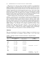
0
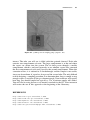
Ln (C/C0) in water
–1
Rep-1
Rep-2
Linear Fit
Linear Regression:
ln(C/C0) = –0.879t
–2
–3
–4
–5
–6
–7
–8
0
1
2
3
Time (hours)
4
5
6
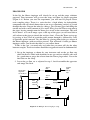
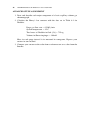
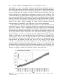
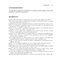
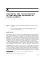
Figure 4-3. Linear transformation of data to obtain the depletion rate constant (Dr).
2:15 104 atmm3/mol, which is in good agreement with literature values
(2:19 104 to 5:48 104 ).
ACKNOWLEDGMENT
I would like to thank Josh Wnuk (Whitman College, Class of 2003) for data
collection and analysis.
REFERENCES
Bamford, H. A., F. C. Ko, and J. E. Baker, Environ. Sci. Technol., 36(20), 4245–4252 (2002).
Charizopoulos, E. and E. Papadopoulou-Mourkidou, Environ. Sci. Technol., 33(14), 2363–2368
(1999).
Cooter, E. J., W. T. Hutzell, W. T. Foreman, and M. S. Majewski, Environ. Sci. Technol., 36(21), 4593–
4599 (2002).
Harmon-Fetcho, J. A., L. L. McConnell, C. R. Rice, and J. E. Baker, Environ. Sci. Technol., 34(8),
1462–1468 (2000).
Mackay, D., W. Y. Shiu, and R. P. Sutherland, Envion. Sci. Technol., 13(3), 333–337 (1979).
Mamontov, A. A., Mamontova, E. A., and E. N. Tarasova, Environ. Sci. Technol., 34(5), 741–747
(2000).
Subhash, S., R. E. Honrath, and J. D. W. Kahl, Environ. Sci. Technol., 33(9), 1509–1515 (1999).
Thurman, E. M. and A. E. Cromwell, Environ. Sci. Technol., 34(15), 3079–3085 (2000).
IN THE LABORATORY
39
IN THE LABORATORY
During the first laboratory period, you will prepare your purge apparatus (Sherer
impinger) and during the following 24 hours take samples to determine the
Henry’s law constant for selected pesticides and PCBs. Your samples (Tenax resin
tubes) can be extracted as you take them or during the beginning of the next
laboratory period. In the second laboratory period you will analyze the sample
extracts on the gas chromatograph and process your data.
Safety Precautions
Safety glasses must be worn at all times during this laboratory experiment.
Most if not all of the compounds you will use are carcinogens. Your
instructor will prepare the aqueous solution of these compounds so that
you will not be handling high concentrations. The purge solution you will be
given contains parts per billion (ppb)-level concentrations and is relatively
safe to work with. You should still use caution when using these solutions
since the pesticides and PCBs are very volatile when placed in water. Avoid
breathing the vapors from this solution.
Extracts of the Tenax tubes should be conducted in the hood since you will
be using acetone and isooctane, two highly flammable liquids.
Chemicals and Solutions
Neat solutions of the following compounds will be used by your instructor to
prepare your aqueous solution:
2,20 -Dichlorobiphenyl
Lindane
4,40 -Dichlorobiphenyl
2,20 ,6,60 -Tetrachlorobiphenyl
Aldrin
2,20 ,4,40 ,6,60 -Hexachlorobiphenyl
3,30 ,4,40 -Tetrachlorobiphenyl
Dieldrin
4,40 -DDD (dichlorodiphenyldichloroethane)
4,40 -DDT (dichlorodiphenyltrichloroethane)
Methoxychlor
Endosulfan I (not added to purge system, but used as a GC internal standard)
You will need, in addition:
Tenax resin, chromatography grade
Deionized water
40
DETERMINATION OF HENRY’S LAW CONSTANTS
Equipment and Glassware
Sherer impingers (one per student group) (available from Ace Glassware;
use the frit that allows gas to exit at the bottom of the impinger)
Pasteur pipets filled with Tenax resin
15-mL glass vials equipped with a Teflon-lined septum (12 per Sherer
impinger setup or student group)
Tygon tubing
Brass or stainless steel fine metering valves
Brass or stainless steel tees
PROCEDURE
41
PROCEDURE
In the lab, the Sherer impinger will already be set up and the purge solutions
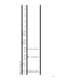
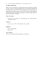
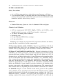
prepared. Your instructor will go over the setup and show its proper operation
(Figure 4-4). Before you start the experiment, you will need to prepare Tenax
resin sampling tubes. Tenax is a resin that has a high affinity for hydrophobic
compounds and will absorb them when water or gas containing analytes is passed
through the resin. Prepare the tubes by taking a glass Pasteur pipet and filling the
narrow end with a small amount of glass wool. Next, place the Tenax resin tube in
the pipet, leaving enough room for more glass wool at the constriction. This will
leave about 1 to 2 cm of empty space at the top of the pipet (we will need this to
add solvent to the pipet to desorb the analytes later). Clean the Tenax resin traps
by passing at least 5 mL of pesticide-grade acetone through it, followed by 5 mL
of pesticide-grade isooctane. Dry the tubes by placing them in the gas stream of
the Sherer impinger (with no analyte present). You will need 14 tubes per Sherer
impinger unless you desorb the tubes as you collect them.
If this is the case, you need only two tubes but you must still dry the tubes
between samples. Tenax resin tubes should be wrapped and stored in aluminum foil.
1. Set up the impinger as shown by your instructor and set the gas flow rate
while the flask is filled with deionized water (no analyte solution) (this will
be a good time to purge the solvent from the Tenax purge tubes). Leave the
final tube on the setup.
2. Leave the gas flow set as adjusted in step 1, but disassemble the apparatus
and empty the flask.
Tenax
tube
Secondary
regulator
set at 50 psi
Pasteur
pipet
Tenax
trap
Cu tubing and
T connectors
Ultrapure N2 or He
Tenax
tube
Fine
metering
valves
Sherer
impinger
Tenax
tube
Tenax
tube
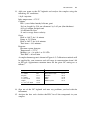
Figure 4-4. Multiple Sherer impinger setup.
42
DETERMINATION OF HENRY’S LAW CONSTANTS
3. Fill the flask with 300 mL of analyte-containing water.
4. Have a stopwatch or clock ready, assemble the Sherer flask, turn the groundglass joint tightly to ensure a seal, and note the time. This is t ¼ 0.
5. Check the flow rate and if needed, adjust it to 0.500 L/min.
6. Sample at the following times to obtain a complete purge profile:
20 minutes
40 minutes
1.00 hour
1.50 hours
2.00 hours
3.00 hours
4.00 hours
5.00 hours
7.00 hours
17.0 hours
29.0 hours
Desorbing the Tenax Resin Tubes
7. Place the Tenax resin tube in a small clamp attached to a ring stand. Lower
the tube so that it just fits into a 15-mL glass vial.
8. Pipet 5.00 mL of pesticide-grade acetone onto the top of the Tenax resin
trap. Allow the acetone to reach the top of the resin with gravity. You may
have to apply pressure with a pipet bulb to break the pressure lock caused
by bubbles in the tube, but be careful not to blow more air into the tube.
After the second or third application (with a bulb) the acetone should flow
with gravity. (The reason for adding acetone is to remove any water from
the resin tube that will not mix or be removed by the hydrophobic
isooctane.)
9. Pipet 5.00 mL of pesticide-grade isooctane onto the resin trap. After the
isooctane has passed through the resin trap, force the remainder of the
isooctane out of the pipet with a bulb. Remove the vial from below the
tube, being careful not to spill any of the contents.
10. Add 10.0 mL of deionized water to the extraction vial and 0.25 g of NaCl.
(NaCl will break any emulsion that forms in the solvent extraction step.)
11. Add 8.0 mL of a 32.70-ppm Endosulfan I (in isooctane) that your instructor
will have prepared for you. Endosulfan I will act as an internal standard for
the gas chromatographic (GC) analysis.
12. Seal the vial and shake it vigorously for 30 seconds. Allow the layers to
separate, transfer 1 to 2 mL of the top (isooctane) layer into a autoinjection
vial, and seal it.
PROCEDURE
43
13. Add your name to the GC logbook and analyze the samples using the
following GC conditions:
1.0-mL injection
Inlet temperature ¼ 270 C
Column:
HP-1 (cross-linked methyl silicone gum)
30.0 m (length) by 530 mm (diameter) by 2.65 mm (film thickness)
4.02-psi column backpressure
3.0-mL/min He flow
31-cm/s average linear velocity
Oven:
Hold at 180 C for 1.0 minute
Ramp at 5.0 C/min
Hold at 265 C for 16.0 minutes
Total time ¼ 34.0 minutes
Detector:
Electron-capture detector
Temperature ¼ 275 C
Makeup gas ¼ Ar with 1 to 5% CH4
Total flow ¼ 60 mL /min
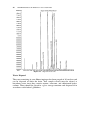
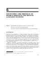
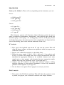
A sample chromatogram is shown in Figure 4-5. Calibration standards will
be supplied by your instructor and will range in concentrations from 1.00
to 500 ppb. Approximate retention times for the given GC setting are as
follows:
Analyte
0
Elution Time (min) Analyte
2,2 -DCB
Lindane
4,40 -DCB
2,20 6,60 -TCB
Aldrin
2,20 ,4,40 ,6,60 -TCB
9.63
12.13
12.71
13.82
16.86
18.86
Elution Time (min)
Endosulfan I (IS)
Dieldrin
DDD
DDT
Methoxychlor
19.75
20.95
22.20
24.72
28.33
14. Sign out of the GC logbook and note any problems you had with the
instrument.
15. Analyze the data and calculate the HLC for all the compounds in your
samples.
44
DETERMINATION OF HENRY’S LAW CONSTANTS
Figure 4-5. Output from the GC.
Waste Disposal
The water remaining in your Sherer impinger has been purged of all analytes and
can be disposed of down the drain. Your sample extracts must be treated as
hazardous waste since they contain acetone, isooctane, and chlorinated hydrocarbons. These should be placed in a glass storage container and disposed of in
accordance with federal guidelines.
ASSIGNMENT
ASSIGNMENT
1. Turn in a diagram of your purge setup.
2. Turn in a spreadsheet showing the HLC calculation.
3. Compare the HLC values calculated to values from the literature.
45
46
DETERMINATION OF HENRY’S LAW CONSTANTS
ADVANCED STUDY ASSIGNMENT
1. Draw and describe each major component of a basic capillary column gas
chromatograph.
2. Calculate the Henry’s law constant with the data set in Table 4-2 for
Dieldrin:
Purge gas flow rate ¼ 0:500 L=min
System temperature ¼ 25 C
Total mass of Dieldrin in flask ðC0 Þ ¼ 725 ng
Volume in Sherer impinger ¼ 300 mL
Mass in each purge interval is in measured in nanograms. Express your
answer in atmm3/mol.
3. Compare your answer to the value from a reference text or a value from the
Internet.
47
0.01389
0.02778
0.04167
0.0625
0.08333
0.125
0.16667
0.20833
0.2917
Purge
Interval Time
(days)
Purge
Interval Time
(hrs)
TABLE 4-2. Sample Data Set
65.16
77.76
73
72.8
69.9
86.9
80.7
76.1
77.5
Mass in Purge
Interval R-1
66.5
74.8
71.9
75.2
70
84.5
69.8
61.6
63
Mass in Purge
Interval R-2
Cummulative
Mass in Purge
Interval R-1
Cummulative
Mass in Purge
Interval R-2
C/Co R1
C/Co R2
ln (C/Co) R1
ln(C/Co) R2
DATA COLLECTION SHEET
5
GLOBAL WARMING:
DETERMINING IF
A GAS IS INFRARED ACTIVE
Purpose: To learn to use an infrared spectrophotometer
To determine if a gas is infrared active
BACKGROUND
Although global warming has drawn growing political attention in recent decades,
relatively few people understand its causes and implications. Global warming has
two faces, one that benefits us and another that may cause serious environmental
and economic damage to the planet. Conditions on Earth would be very different
without the greenhouse effect of atmospheric warming. Natural atmospheric
gases, including carbon dioxide and water vapor, are responsible for adjusting
and warming our planet’s atmosphere to more livable conditions. In fact, there is
one popular theory that the Earth is actually a living organism and that under
normal conditions (without human interference), the Earth will maintain the lifesustaining environment that it has acquired over the last 100 million years or so.
This theory is the Gaia hypothesis proposed by James Lovelock, and there are
several short books on the subject.
The bad side, the anthropogenic side, of global warming is still strongly
debated between some politicians and scientists, but it is generally well accepted
among scientists that humans are contributing exponentially to the warming of the
planet. Unfortunately, some governments and political parties side with the
Environmental Laboratory Exercises for Instrumental Analysis and Environmental Chemistry
By Frank M. Dunnivant
ISBN 0-471-48856-9 Copyright # 2004 John Wiley & Sons, Inc.
49
50
GLOBAL WARMING: DETERMINING IF A GAS IS INFRARED ACTIVE
economists, who often have little knowledge of the science behind the argument
but are concerned primarily with constant economic growth rather than sustained
growth. This bad side to global warming has been studied for several decades and
data from these studies is presented below.
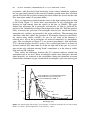
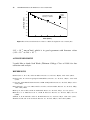
First, it is important to understand the nature of the light coming from our Sun
to the Earth. Figure 5-1 shows three representations of the wavelengths and
intensity of light coming from the surface of the Sun (at 5900 K). The upper
dashed line represents the wavelengths and intensity of light as predicted by
physicists for a blackbody residing at the temperature of the sun. This line predicts
fairly accurately the spectrum of wavelengths observed just outside the Earth’s
atmosphere by satellites (represented by the upper solid line). The remaining line
(the lower solid line) shows the spectrum of wavelengths detected at the Earth’s
sea surface using similar satellites. As you can see, some of the intensity is
reduced and a few of the wavelengths are removed completely by atmospheric
gases. The wavelengths in Figure 5-1 are given in micrometers, with ultraviolet
(UV) radiation between 0 and 0.3 on the x axis, visible light from 0.3 to about 0.8
and near-infrared (IR) from about 0.8 to the far right side of the plot. As you see,
most of the solar radiation entering Earth’s atmosphere is in the form of visible
light and near-IR radiation.
Next, notice the difference between the UV radiation intensity outside the
atmosphere and at sea level. These wavelengths, which cause damage to skin and
other materials, are removed in the stratosphere during the formation of ozone
shown below (diatomic oxygen absorbs these wavelengths, splits into free oxygen
0.25
Energy Density H2 (W/m2 ⋅ Å)
0.20
Solar Irradiation Curve Outside Atmosphere
Solar Irradiation Curve at Sea Level
Curve for Blackbody at 5900 °K
0.15
O3
0.10
H2O
H2O
H2O
H2O
0.05
O2
0
H2O
O2, H2O
0
H2O, CO2
H2O, CO2
H2O, CO2
0.2 0.4 0.6 0.8 1.0 1.2 1.4 1.6 1.8 2.0 2.2 2.4 2.6 2.8 3.0 3.2
Wavelength (µm)
Figure 5-1. Wavelengths and intensity of wavelengths of radiation emitted by the sun and reaching
Earth’s sea surface. (From Department of the Air Force, 1964.)
BACKGROUND
51
radicals, and binds to another O2 to form O3). This is the source of concern with
chlorofluorohydrocarbons, which interfere with this process and promote the
destruction of O3, thus allowing more high energy UV to reach Earth’s surface.
O2 ðgÞ þ hn ! 2O2 ðgÞ
O2 ðgÞ þ O2 ðgÞ þ M ! O3 ðgÞ þ M ðgÞ þ heat
Visible light is also attenuated significantly by Earth’s atmosphere, but not to
the extent that it limits the growth of plant life. Some of the visible light is simply
absorbed and rereleased as heat in the atmosphere. Other visible wavelengths are
scattered and reflected back into space, which is why the astronauts can see the
Earth from space. Several compounds in the atmosphere partially or completely
absorb wavelengths in the near-IR radiation on the left side of the figure.
Absorption of these wavelengths is represented by the shaded areas for O3,
H2O, O2, and CO2. This is one mechanism of global warming, in which the
atmosphere is heated by IR radiation incoming from the Sun rather than reradiated
from Earth’s surface. To fully understand the importance of these gases in global
warming, we must also look at the type of radiation the Earth is emitting.
As visible light reaches Earth’s surface, it is absorbed by the surface and
transformed into heat. This heat is reemitted back into the atmosphere and space
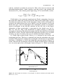
by Earth. When physicists estimate the wavelengths and intensity of wavelengths
for Earth as a blackbody at 320 K, the dashed-line spectrum shown in Figure 5-2
results. Note that the wavelengths released by Earth are much longer wavelength
(far, far to the right of the wavelengths shown in Figure 5-1). These far-infrared
Radiance (mW/m ⋅ sr ⋅ cm–1)
320 K
150
100
H2O
atm
window
O3
CO2
CH4
50
H2O
0
400
600
800
1000
1200
1400 1500
–1)
Wavenumber (cm
25
15
10
7.5
Wavelength (µm)
Figure 5-2. Wavelengths and intensity of wavelengths of radiation emitted by the Earth. (From
Hanel et al., 1972.)
52
GLOBAL WARMING: DETERMINING IF A GAS IS INFRARED ACTIVE
wavelengths are very susceptible to being absorbed by atmospheric gases, as
indicated by the decrease in intensity shown by the solid line. The solid line shows
the wavelength and intensity of wavelengths measured by a satellite above Earth’s
surface, but this time the satellite is pointed at Earth instead of the Sun. Note the
strong absorbance by atmospheric constituents, primarily water, methane, and
carbon dioxide. By absorbing the IR radiation instead of letting it pass freely into
space, the gases heat Earth’s atmosphere. The amount of global warming resulting
from the reflected IR radiation is related directly to the concentration of atmospheric gases that can absorb the emitted IR radiation. Before we can evaluate the
cause of the ‘‘bad’’ global warming, we must look at historical data on
concentrations of greenhouse gases (IR-active gases) in the atmosphere.
In the 1950s the U.S. government initiated a project to collect baseline data on
planet Earth. One of the most important studies was to monitor the concentration
of CO2 in a remote, ‘‘clean’’ environment. The site selected for this monitoring
program was the observatory on Mauna Loa in Hawaii. This site was selected for
its location in the middle of the Pacific, away from major pollution sources, and
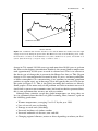
for its high altitude (about 14,000 feet). Data from this monitoring program are
shown in Figure 5-3 and are available from the LDEO Climate Data Catalog,
which is maintained by the International Research Institute at Columbia University (http://www.ingrid.ldgo.columbia.edu/). Data from 1958 to the
year 2000 (not shown) consistently show an increase in atmospheric CO2
concentrations. In addition, for the first time we can actually see the Earth
‘‘breath,’’ as indicated in the inset in Figure 5-3: In the summer, when plant
growth is highest in the northern hemisphere, CO2 levels are at a minimum. This
is followed by fall, when plant growth is subsiding and dying, and CO2 levels start
to increase. The CO2 concentration reaches a maximum in winter, followed by a
decrease in spring as plants start growing again to repeat the cycle.
Figure 5-3. CO2 measurements from Mauna Loa. (Data from http://ingrid.ldgo.
columbia.edu/.)
BACKGROUND
53
One problem with the data set from Mauna Loa is that it represents only a
small snapshot in time; with issues such as global warming, we must look at longterm geological time scales. To do this, scientists have collected ice cores from a
variety of places across the Earth. Ice cores represent a long history of atmospheric data. As snow falls over cold areas and accumulates as snow packs and
glaciers, it encapsulates tiny amounts of atmospheric gases with it. When ice
cores are taken and analyzed carefully, they can give information on the
composition of the atmosphere at the time the snow fell on the Earth. An example
of these data for the Vostok ice core is shown in Figure 5-4. This data set goes
back in time 160,000 years (from left to right) from the present and gives us a
long-term idea of the composition of the atmosphere. The three figures show the
concentration of CH4 with time (Fig. 5.4a), the concentration of CO2 with time
(Fig. 5.4b), and the estimated temperature with time (Fig. 5.4c). The CH4 and CO2
data are self-explanatory and are simply the gases trapped in the glacier, but the
temperature data are a bit more complicated. To estimate the temperature as a
function of time, scientists look at the abundance of the oxygen-18 isotope in
glacial water. Water on Earth contains mostly oxygen-16, but a small amount of
oxygen-18 is present. During warmer geologic times on Earth, more water
containing 18O is evaporated from the oceans and falls as snow over cold regions.
In contrast, cooler geologic times will have less 18O in the atmospheric and snow.
By conducting experiments we can estimate how much 18O is present at a given
temperature and estimate what the temperature was when each layer of the glacial
water was deposited. This allows Figure 5-4c to be created. When the three figures
are compared, a strong correlation between high CH4 concentrations, high CO2
concentrations, and high temperature is noticed. This can be understood by
Figure 5-4. ðaÞ CH4, ðbÞ CO2, and ðcÞ temperature data from the Vostok ice core study. (Data from
http://ingrid.ldgo.columbia.edu/.)
GLOBAL WARMING: DETERMINING IF A GAS IS INFRARED ACTIVE
Change in Temperature (°C) Relative to Present
54
4
2
0
–2
–4
–6
–8
–10
0
20000
40000
60000 80000 100000 120000 140000 160000
Age (years)
(c)
Figure 5-4. ðContinued Þ
returning to Figures 5-1 and 5-2 and noting which gases absorb or trap energy in
Earth’s atmosphere.
Now we combine the CO2 data from the Vostok ice core and the Mauna Loa
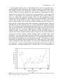
data set to create Figure 5-5. Note in the figure that the direction of time changes,
going back in time from left to right. This figure contains data going back 160,000
years, and we notice two distinct spikes in CO2 concentration (and in temperature
if we look again at Figure 5-4). The important point to note in Figure 5-5 is the
rate at which the CO2 (and temperature) has changed over time. The natural
BACKGROUND
55
400
{
350
300
250
200
150
100
Vostok Ice Core Data
CO2 Concentration (ppmv)
Mauna Loa Data Set
50
0
150000
100000
50000
0
Years in the Past
Figure 5-5. Combined data from the Vostok ice core and the Mauna Loa studies. Note the rapid
change in CO2 levels during the present time. The Mauna Loa data are from Keeling (1995, 1996);
the Vostok ice core data are from Barnola et al. (1987), Genthon et al. (1987), and Jouzel et al.
(1987). (Data from http://ingrid.ldgo.columbia.edu/.)
change in CO2 around 130,000 years ago took more than 30,000 years to go from
the lowest to the highest concentration. Similarly, the recent climb in temperature
took approximately 20,000 years to reach its current level. This is in contrast to
the drastic rate of change that is present in the Mauna Loa data set. This 50-ppm
change in CO2 concentration has occurred in only 50 years, and most predictions
of future atmospheric CO2 concentrations (if we continue to consume petroleum
products at current rates) are in the range 700 to 800 ppm by the year 2100 (locate
this point in Figure 5-5). This is the global warming that concerns us directly.
Some people call for more study of the problem and wish to maintain our use of
fossil fuels to preserve our economic status, but based on the data presented here,
this is one experiment that we may not wish to conduct.
Although many scientists accept that global temperatures are rising, they are
less in agreement about the effects of global warming, Most, however, agree on
the following predictions:
Warmer temperatures (averaging 5 to 10 C by the year 2100)
Loss of coastal areas to flooding
Damage to coral reefs (bleaching)
Increased incidence of violent weather
Increased outbreaks of diseases (new and old)
Changing regional climates (wetter or drier, depending on where you live)
56
GLOBAL WARMING: DETERMINING IF A GAS IS INFRARED ACTIVE
O C O
O C
(a)
O
O
(b)
C O
O C O
(c)
(d)
Figure 5-6. Vibrational structures for CO2.
THEORY
In the background section we saw which greenhouse gases absorb IR radiation
and at what wavelengths. But what actually makes a gas IR active? There are two
prerequisites for a gas to be IR active. First, the gas must have a permanent or
temporary dipole. Second, the vibration of the portion of the molecule having the
dipole must be at the same frequency as the IR radiation that is absorbed. When
these two criteria are met, the gas molecule will absorb the radiation, increase its
molecular vibrations, and thus retain the heat in the atmosphere. This is why gases
such as O2 and N2 are not IR active; they do not have permanent or sufficiently
temporary dipoles. Molecules such as chlorofluorocarbons (CFCs), on the other
hand, have permanent dipoles and are very IR active (actually, this is the only
connection between global warming and ozone depletion—CFCs are active in
both cases). However, what about symmetrical molecules such as CO2 and CH4?
To understand how these molecules are IR active, we must draw their molecular
structures.
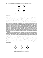
Figure 5-6 shows several possible vibrational structures for CO2. The arrows
indicate the direction of the stretch. Figure 5-6a is the normal way we think about
CO2, with each carbon–oxygen bond stretching in unison and away from the
central carbon atom and no dipole present in the molecule. However, the stretches
in Figure 5-6b, c, and d are also possible and result in a temporary dipole that can
absorb IR radiation. Similar observations can be made for methane (Figure 5-7).
The symmetrical orientation is shown in Figure 5-7a, while asymmetrical
molecules are shown in Figure 5-6b and c, which contain temporary dipoles.
The latter two molecules absorb IR radiation and result in a heating of the
atmosphere.
H
H
C
H
H
H
C
H
H
H
C
H
H
H
(a)
(b)
(c)
H
Figure 5-7. Molecular vibrations for methane.
REFERENCES
57
ACKNOWLEDGMENT
I would like to thank Dr. Paul Buckley for taking the IR readings given in the
instructor’s version of this manual.
REFERENCES
Barnola, J. M., D. Raynaud, Y. S. Korotkevich, and C. Lorius, Nature, 329, 408–414 (1987).
Berner, E. K. and R. A. Berner, Global Environment: Water, Air, and Geochemical Cycles, Prentice
Hall, Upper Saddle River, NJ, 1996, p. 32.
Department of the Air Force, Handbook of Geophysics and Space Environmental, 1965, p. 16–2.
Genthon, C., J. M. Barnola, D. Raynaud, C. Lorius, J. Jouzel, N. I. Barkov, Y. S. Korotkevich, and V.
M. Kotlyakov, Nature, 329, 414–418 (1987).
Hanel, R. A., B. J. Conrath, V. G. Kunde, C. Prabhakara, I. Revah, V. V. Salomonson, and G. J.
Wolfrod, J. Geophys. Res., 77(15), 2629–2641 (1972).
Houghton, J. T., F. J. Jenkins, and J. J. Ephraums (eds.), Climate Change: The IPCC Scientific
Assessment, Cambridge University Press, Cambridge, 1990.
Houghton, J. T., L. G. Meira Filho, B. A. Callander, N. Harris, A. Katterberg, and K. Maskell (eds.)
Climate Change: The Science of Climate Change, The IPCC Scientific Assessment, Cambridge
University Press, Cambridge, 1995.
Jager, J. and F. L. Ferguson (eds.), Climate Change: Science, Impacts, and Policy, Proceedings of the
2nd World Climate Conference, Cambridge University Press, Cambridge, 1991.
Jouzel, J., C. Lorius, J. R. Petit, C. Genthon, N. I. Barkov, V. M. Kotlyakov, and V. M. Petrov, Nature,
329, 403–408 (1987).
Keeling, C. D., T. P. Whorf, M. Wahlen, and J. van der Plicht, Nature, 375, 666–670 (1995).
Keeling, C. D., J. F. S. Chine, and T. P. Whorf, Nature, 382, 146–149 (1996).
LDEO Climate Data Catalog, maintained by International Research Institute (IRI) at Columbia
University, http://www.ingrid.ldgo.columbia.edu/.
Mintzer, I. M. (ed.), Stockholm Environmental Institute, Confronting Climate Change: Risks,
Implications, and Responses, Cambridge University Press, Cambridge, 1992.
Skoog, D. A., F. J. Holler, and T. A. Nieman (eds.), Principles of Instrumental Analysis, 5th ed.,
Saunder College Publishing, Philadelphia, 1998.
World Resources Institute, World Resources, 1996–1997, Oxford University Press, Oxford, 1996.
58
GLOBAL WARMING: DETERMINING IF A GAS IS INFRARED ACTIVE
IN THE LABORATORY
There is no exact procedure for conducting this laboratory other than consulting
the users’ guide for your IR instrument. Sign in the instrument logbook and
remember to record any problems with the instrument when you finish. You will
be provided with a variety of gases that you will measure on your IR instrument.
Print out the spectrum for each gas and use the resources in your library to
determine what type of vibration is occurring at each wave number where you
observe absorption of IR radiation.
Safety Precautions
Avoid the use of methane or other flammable gases around electronic
equipment or flames.
Chemicals
Gases: N2, O2, a CFC, a CFC substitute, CO2, and CH4
Equipment
IR spectrophotometer
IR gas cell
Waste Disposal
The gas cells should be filled and emptied in a fume hood.
ASSIGNMENT
59
ASSIGNMENT
Turn in your IR spectrum and label each peak with respect to the vibration that is
occurring.
60
GLOBAL WARMING: DETERMINING IF A GAS IS INFRARED ACTIVE
ADVANCED STUDY ASSIGNMENT
1. What are the requirements for a gas to be IR active?
2. Look up the composition of Earth’s atmosphere. Which gases would you
expect to be IR active?
3. Draw a diagram of a basic IR instrument and explain how it works.
4. Using the Internet, find how much CO2 is emitted each year by the most
productive nations. Which nation has the largest emissions?
6
MONITORING THE PRESENCE OF
HYDROCARBONS IN AIR AROUND
GASOLINE STATIONS
Purpose: To determine the exposure of citizens to gasoline vapors
To learn to use a personal sampling pump
To learn to analyze gasoline components on a gas chromatograph
BACKGROUND
Each day we are exposed to a variety of organic vapors. Yet we experience
perhaps the greatest level of exposure when we fill our automobiles with gasoline.
Gasoline contains a variety of alkanes, alkenes, and aromatics. In California
alone, it has been estimated that 6,100,000 lb of gasoline vapors per year are
released into the atmosphere (http://www.arb.ca.gov). It is also interesting
to note that at least 23 of the 1430 National Priorities List sites (compiled by the
U.S. Environmental Protection Agency) contain automotive gasoline (http://
www.atsdr.cdc.gov).
Table 6-1 shows the approximate composition of unleaded gasoline. You
should note several carcinogens in this list. The right-hand column shows data
on exposure limits (http://www.bpdirect.com); the allowed concentrations
shown are relatively high compared to some pollutant exposures, but if you
consider how often you (or the gas station attendant) are exposed to these vapors,
you may start to appreciate the problem and potential cancer risk.
Environmental Laboratory Exercises for Instrumental Analysis and Environmental Chemistry
By Frank M. Dunnivant
ISBN 0-471-48856-9 Copyright # 2004 John Wiley & Sons, Inc.
61
62
MONITORING THE PRESENCE OF HYDROCARBONS IN AIR
TABLE 6-1. Composition of Unleaded Gasoline
Component
Benzene
Butane
Cyclohexane
Ethylbenzene
Heptane
Hexane
Pentane
Toluene
Trimethylbenzene
Xylene
Percent Range
by Weight
0–3
4–6
0–1
0–2
6–8
6–8
9–11
10–12
0–3
8–10
Exposure Limits
(ppm)
1–5
800
300
100–125
400–500
50–500
600–1000
100–200
25
100
Source: http://www.bpdirect.com
But what exactly are the risks of exposure? Laboratory animals (rats and mice)
exposed to high concentrations of gasoline vapors (at 67,262 and 2056 ppm)
showed kidney damage and cancer of the liver. n-Heptane and cyclohexane can
cause narcosis and irritation of the eyes and mucous membranes. In studies using
rabbits, cyclohexane caused liver and kidney changes. Benzene, a known human
carcinogen, has an eight-hour exposure limit of 0.5 ppm. Studies have shown that
exposure to benzene vapor induce leukemia at concentrations as low as 1 ppm.
Trimethylbenzene (isooctane) has an eight-hour exposure limit of 25 ppm and
above this limit can cause nervousness, tension, and anxiety as well as asthmatic
bronchitis. n-Hexane has been shown to cause peripheral nerve damage and
hexanes show narcotic effects at 1000 ppm. Toluene can cause impairment of
coordination and momentary memory loss at 200 to 500 ppm. Palpations, extreme
weakness, and pronounced loss of coordination can occur at 500 to 1500 ppm.
The eight-hour exposure limit for toluene is 100 ppm. (Data in this paragraph
were obtained from http://www.brownoil.com.)
As you can see from the discussion above, exposure to gasoline vapors,
although routine, should be of concern to anyone filling his or her automobile’s
gas tank.
THEORY
The sampling of gasoline vapors is a relatively easy process. Figure 6-1 shows a
typical sampling pump and sample cartridge. The pump comes calibrated from
the factory with respect to airflow, and the flow can be adjusted on most pumps.
The pump pulls the air and vapors through the sampling tube, thus avoiding both
contamination of the sample tube with compounds from the pump and contamination of the sampling pump with gasoline vapors. A variety of sample tubes are
available, with difference resins designed for efficient adsorbance of analytes of
REFERENCES
63
Figure 6-1. Q-Max personal sampling pump. (Supelco, Inc.)
interest. The tube you will use is filled with fine-grained charcoal. Each tube
contains two compartments of resin. The large compartment is at the end where
the vapors are drawn into the system. The air then passes through a smaller
compartment, which is analyzed separately to see whether vapors have saturated
the first compartment of resin and passed to the second compartment. When this
saturation occurs, it is referred to as breakthrough, and the sample is not usable,
since you do not know if vapor has also passed the second tube. The only difficult
task in designing a sampling procedure is to determine how long to sample to trap
enough vapors to analyze on the gas chromatograph. Your instructor will specify
how long you should sample but typically a 5 to 10 minute sample will suffice.
You will also be using decane as an internal standard for the GC. Your instructor
will review the use of this approach at the beginning of the laboratory.
REFERENCES
http://www.arb.ca.gov, accessed Oct. 5, 2003.
http://www.atsdr.cdc.gov, accessed Oct. 5, 2003.
http://www.bpdirect.com, accessed Oct. 5, 2003.
http://www.brownoil.com, accessed Oct. 5, 2003.
http://www.cdc.gov/niosh/homepage.html, accessed Oct. 5, 2003.
64
MONITORING THE PRESENCE OF HYDROCARBONS IN AIR
IN THE LABORATORY
You will be divided into groups and sent to a local gasoline station to take
samples. Your instructor will have already contacted the owner of the station and
asked for permission. You may actually fill cars with gasoline, or you may simply
stand beside car owners (or station attendants) as they operate the pumps. Next,
you will extract the samples and analyze them on the GC. There are many
compounds present in gasoline, but we will only be analyzing selected compounds.
Safety Precautions
Safety glasses must be worn when in the laboratory.
All of these vapors have exposure limits, and many are carcinogens. Avoid
exposure to these vapors in the laboratory by working in fume hoods. Your
instructor may choose to use carbon disulfide, a highly toxic and cancercausing agent. Always work in the fume hood with this solvent, even when
filling the syringe for injection into the GC.
Chemicals and Solutions
We will analyze for the compounds shown in Table 6-2. Decane will be used as
the internal standard that will be added to your desorption (extraction) solvent
(pentane or carbon disulfide) as well as the GC calibration standards at a
concentration of 29.2 ppm. You will use the density to calculate the concentration
in your calibration standards (volume added times density equals mass added to
volumetric).
Use the data shown in Table 6-3 to prepare your GC calibration standards if
these standards are not provided from the stockroom. The solvent used for your
samples and standards will be pentane or carbon disulfide containing the same
concentration of decane as used in the calibration standards. You will also need
approximately 50 mL of internal standard solution for extraction of your samples
from the charcoal. Your instructor may also have this solution prepared.
TABLE 6-2. Density of Compounds to Be Used in Calibration Standards
Compound
Benzene
Ethyl benzene
n-Heptane
Isooctane
Toluene
Density
(g/mL or mg/mL)
0.8787
0.866
0.684
0.6919
0.866
Compound
Density
(g/mL or mg/mL)
m-Xylene
o-Xylene
0.8684
0.8801
Decane
0.73 (internal standard)
65
50
Decane
36.5
43.935
43.3
34.2
34.595
43.3
43.42
44.005
Mass (mg)
in Vol.
1460
1757.4 ppm
1732
1368
1383.8
1732
1736.8
1760.2
Stock
Conc. in
25-mL Vol.
29.2
3.5148
3.464
2.736
2.7676
3.464
3.4736
3.5204
Std. 1
1 : 50 Dilution,
Then 1 : 10
29.2
7.0296
6.928
5.472
5.5352
6.928
6.9472
7.0408
Std. 2
1 : 50 Dilution
Then 2 : 10
29.2
17.574
17.32
13.68
13.838
17.32
17.368
17.602
Std. 3
1 : 50 Dilution,
Then 5 : 10
29.2
35.148
34.64
27.36
27.676
34.64
34.736
35.204
Std. 4
1 : 50
Dilution
29.2
70.296
69.28
54.72
55.352
69.28
69.472
70.408
Std. 5
1 : 25
Dilution
a
Use the densities shown in Table 6-2. Concentrations of analytes in standards 1–5 are in ppm. Note that the concentrations of Decane should be the same (29.2 ppm) in all standards
and sample extracts.
50
50
50
50
50
50
50
Benzene
Ethyl Benzene
n-Heptane
Isooctane
Toluene
m-Xylene
o-Xylene
Compound
mL Neat to a
25-mL Vol.
TABLE 6-3. Solutions for Making Calibration Standards from Pure (Neat) Compoundsa
66
MONITORING THE PRESENCE OF HYDROCARBONS IN AIR
TABLE 6-4. Approximate Retention Times for Analytes on a
DB-1 Column
Analyte
Benzene
Ethyl Benzene
n-Heptane
Isooctane
Retention Time
(min)
4.52
10.67
6.33
5.95
Analyte
Toluene
m-Xylene
o-Xylene
Retention Time
(min)
8.05
10.88
11.43
GC Conditions
Splitless for the first 2 minutes, split mode for the reminder of the analysis
Injector temperature: 250 C
Detector temperature: 310 C
Oven: Initial temp 40 C
Hold for 5 minutes
Ramp at 10 C/min to 200 C
Hold for 5 minutes (or less)
Column: DB-1 or DB-5
Injection volume: 1 mL
Integrator settings: Attenuation 3
Threshold 3
Retention times (Table 6-4)
Equipment and Glassware
10-mL Teflon-septum capped vials for extracting sample charcoal
Needle-nosed pliers for breaking the sample containers
Capillary column gas chromatograph
1-, 2-, and 5-mL volumetric pipets
PROCEDURE
67
PROCEDURE
Week 1
1. Your instructor will assign you times and dates to sample at a local gasoline
filling station. Each group will take one sample. Use a piece of plastic tubing
to position the sample point at shoulder level.
2. If you are using carbon disulfide as your extraction solvent, take a sample
over a 5 to 10 minute period. It typically takes 0.75 to 1.5 minutes to fill an
empty tank, so you will have to take a composite sample while filling several
cars. Remember to turn the pump off between cars. If you are using pentane
as your extraction solvent, you will need to sample for 10 minutes.
3. Cap the ends of the sampling tube with the caps included in your kit when
you are finished.
Week 2
4. Start the GC, and run your calibration standards while you prepare your
samples.
5. Extract (desorb) your sample tubes as illustrated by your laboratory
instructor. You will need to place the charcoal from the front and back in
two separate vials.
6. Add 1.00 mL of your extraction solvent containing decane (your internal
standard).
7. Cap the vial and allow it to stand for 5 minutes.
8. Analyze each sample on the GC.
Waste Disposal
All extraction solvents, calibration standards, and liquid waste should be collected
in an organic waste container and disposed of by your chemistry stockroom. Your
sample tubes can be disposed of in the broken-glass container.
68
MONITORING THE PRESENCE OF HYDROCARBONS IN AIR
ASSIGNMENT
1. Calculate the concentration of each analyte in an extract and the total mass
of each analyte in your extraction vial.
2. Use the flow rate and sample period to convert the total mass collected to the
average concentration in the air (mg/m3 or ng/m3).
3. Does your dose exceed the limit mentioned in the background material?
ADVANCED STUDY ASSIGNMENT
ADVANCED STUDY ASSIGNMENT
1. Draw and label a basic capillary column gas chromatograph.
2. Describe each major component in one to three sentences.
69
DATA COLLECTION SHEET
PART 3
EXPERIMENTS FOR WATER SAMPLES
7
DETERMINATION OF
AN ION BALANCE
FOR A WATER SAMPLE
Purpose: To determine the ion balance of a water sample and learn to perform
the associated calculations
To learn the use of flame atomic absorption spectroscopy unit
To learn the use of an ion chromatograph unit
BACKGROUND
A favorite cartoon from my childhood shows Bugs Bunny preparing water from
two flasks, one containing Hþ ions and another containing OH ions. Although
this is correct in theory, only Bugs could have a flask containing individual ions.
In reality, counterions must be present. For example, in highly acidic solutions,
the Hþ ions are in high concentration but must be balanced with base ions, usually
chloride, nitrate, or sulfate. In high-pH solutions, the OH ions are balanced by
cations such as Naþ, Kþ, or Ca2þ. The combined charge balance of the anions and
cations must add up to zero in every solution. This is the principle behind the
laboratory exercise presented here. You will analyze a water solution for anions
by ion chromatography (IC) and for cations by flame atomic absorption spectroscopy (FAAS) and use these data to determine the ion balance of your solution. Of
course, this exercise is easier than in real life, where you would have no idea
which ions are present and you would have to analyze for every possible cation
and anion. In this exercise we tell you which anions and cations are present.
Environmental Laboratory Exercises for Instrumental Analysis and Environmental Chemistry
By Frank M. Dunnivant
ISBN 0-471-48856-9 Copyright # 2004 John Wiley & Sons, Inc.
73
74
DETERMINATION OF AN ION BALANCE FOR A WATER SAMPLE
The presence of a variety of cations and anions in solution is very important to
organisms living in or consuming the water. For example, we could not live by
drinking distilled or deionized water alone. We need many of the ions in water to
maintain our blood pressure and the ion balance in our cells. This need for ions in
solution is important even for microorganisms living in water, since water is their
medium of life. In distilled water, microbial cells try to balance the ionic strength
between the internal (cell) and external water. In doing so in distilled water, the
microbe cell will expand and could rupture, due to the increased volume of water
required to balance the osmotic pressure across the cell membrane.
Another important point concerning ionic strength is the toxicity of inorganic
pollutants, specifically metals and nonmetals. In general, the predominant toxic
form of inorganic pollutants is their hydrated free ion. However, notable exceptions to this rule include organic forms of mercury and the arsenic anion.
Inorganic pollutants are also less toxic in high–ionic strength (high-ion-containing) waters, due to binding and association of the pollutant with counterions in
solution. This is called complexation and is the focus of computer models such as
Mineql, Mineqlþ, and Geochem. For example, consider the toxicity of the
cadmium metal. The most toxic form is the Cd2þ ion, but when this ion is
dissolved in water containing chloride, a significant portion of the cadmium will
be present as CdClþ, a much less toxic form of cadmium. Similar relationships
occur when other anions are present to associate with the free metal.
THEORY
When the concentration of all ions in solution is known, it is relatively easy to
calculate an ion balance. An example is shown in Table 7-1 for a river water
TABLE 7-1. Example Calculation of the Electroneutrality of a Hypothetical River
Water Sample
Ion
Cations
Ca2þ
Mg2þ
Naþ
Kþ
Molar Concentration
(mol/L)
3:8 104
3:4 104
2:7 104
5:9 105
Charge Balance
Total
Ion Balance
7:6 104
6:8 104
2:7 104
5:9 105
Total cations:
Anions
HCO
3
Cl
F
SO2
4
NO
3
9:6 104
2:2 104
5:3 106
1:2 104
3:4 104
Source: Adapted from Baird (1995).
1:77 103
9:6 104
2:2 104
5:3 106
2:4 104
3:4 104
Total anions:
1:77 103
Net difference: 0:00 103
REFERENCES
75
sample. In the data analysis for this laboratory report, you must first convert from
mg/L to molar concentration. Cations and anions in Table 7-1 are separated into
two columns, and each molar ion concentration is multiplied by the charge on the
ion. For calcium, the molar concentration of 3:8 104 is multiplied by 2 because
calcium has a þ2 charge. The molar charges are summarized, and if all of the
predominant ions have been accounted for, the difference between the cations and
anions should be small, typically less than a few percent of the total concentration.
A sample calculation is included in the Advanced Study Assignment. Note that an
important step in going from your analyses to your final ion balance number is to
account for all dilutions that you made in the lab.
REFERENCES
Baird, C., Environmental Chemistry, W.H. Freeman, New York, 1995.
Berner, E. K. and R. A. Berner, Global Environment: Water, Air, and Geochemical Cycles, Prentice
Hall, Upper Saddle River, NJ: 1996.
Dionex DX-300 Instrument Manual.
76
DETERMINATION OF AN ION BALANCE FOR A WATER SAMPLE
IN THE LABORATORY
Safety Precautions
As in all laboratory exercises, safety glasses must be worn at all times.
Use concentrated HNO3 in the fume hood and avoid breathing its vapor. For
contact, rinse your hands and/or flush your eyes for several minutes. Seek
immediate medical advice for eye contact.
Glassware
Standard laboratory glassware: class A volumetric flasks and pipets
Chemicals and Solutions
ACS or reagent-grade NaCl, KCl, MgSO4, NaNO3, and Ca(NO3)2 (salts
should be dried in an oven at 104 C and stored in a desiccator)
1% HNO3 for making metal standards
Deionized water
0.2-mm Whatman HPLC filter cartridges
0.2-mm nylon filters
Following are examples of preparation of IC regenerate solutions and eluents;
consult the user’s manual for specific compositions.
IC Regenerate Solution (0.025 N H2SO4). Prepare by combining 1.00 mL of
concentrated H2SO4 with 1.00 L of deionized water. The composition of this
solution will vary depending on your instrument. Consult the user’s manual.
IC Eluent (1.7 mM NaHCO3/1.8mM Na2CO3). Prepare by dissolving 1.4282 g
of NaHCO3 and 1.9078 g of Na2CO3 in 100 mL of deionized water. This 100-fold
concentrated eluent solution is then diluted with 10.0 mL diluted to 1.00 L of
deionized water and filtered it through a 0.2-mm Whatman nylon membrane filter,
for use as the eluent. Store the concentrated solution at 4 C. Deionized water is
also a reagent for washing the system after completion of the experiment. For
each run, set the flow rate at 1.5 mL/min. The total cell value while running
should be approximately 14 mS. Inject one or two blanks of deionized water
before any standards or water samples, in order to achieve a flat baseline with a
negative water peak at the beginning of the chromatogram. The composition of
these solutions will vary depending on your instrument. Consult the user’s manual.
IC Standards. Prepare a stock solution of the anions present in the synthetic
water (chloride, nitrate, and sulfate) for each anion. For chloride, 0.208 g of NaCl
should be dissolved in 100.0 mL of deionized water, yielding 1.26 g of Cl/L.
Dilute this stock Cl solution 1 : 10 to give 0.126 g or 126 mg of Cl per litre of
working standard. For nitrate, dissolve 0.155 g of Ca(NO3)2 in 100.0 mL of
IN THE LABORATORY
77
deionized water to yield 1172 mg NO
3 /L. For the sulfate stock solution, dissolve
15.113 g of MgSO4 in 100.0 mL of deionized water to yield 120,600 mg of SO2
4 /
L. An additional 1 : 1 100 mL dilution of the sulfate stock may aid in the
preparation of lower-concentration sulfate standards. Thus, the working stock
solution concentrations of the anions are
126 ppm Cl
1172 ppm NO
3
1206 ppm SO2
4
IC standards are made from the stock solutions by dilutions using 100-mL
volumetric flasks and the appropriate pipets. Each calibration level shown below
contains all three anions in one 100-mL volumetric flask. Final solutions should
be stored in plastic bottles to prevent deterioration of the standards.
Calibration Standard I: 0.063 ppm Cl, 0.565 ppm NO
3 , and 0.603 ppm
2
SO4 . Make a 0.05 : 100 dilution of chloride stock and nitrate stock using a
50.0- or 100.0-mL syringe and a 100 mL volumetric flask. Make a 0.05 : 100
dilution of the 1206-ppm sulfate solution using a 50.0- or 100.0-mL syringe and
fill to the 100-mL mark with deionized water.
Calibration Standard II: 0.252 ppm Cl, 1.13 ppm NO
3 , and 1.21 ppm
.
Make
a
0.2
:
100
dilution
of
chloride
stock
using
a
500.0-mL
syringe, a
SO2
4
0.1 : 100 dilution of nitrate stock using a 250.0-mL syringe, and a 0.1 : 100 dilution
of the 1206-ppm sulfate solution using a 100.0-mL syringe. Fill to the 100-mL
mark with deionized water.
Calibration Standard III: 1.26 ppm Cl, 5.65 ppm NO
3 , and 6.03 ppm
.
Make
by
a
1
:
100
dilution
of
chloride
stock,
a
0.5
:
100
dilution of nitrate
SO2
4
stock using a 500.0-mL syringe, and a 0.5:100 1206-ppm sulfate solution using a
500.0-mL syringe. Fill to the 100-mL mark with deionized water.
Calibration Standard IV: 2.52 ppm Cl, 11.3 ppm NO
3 , and 12.06 ppm
.
Make
by
a
2
:
100
dilution
of
chloride
stock,
a
1:100
dilution of nitrate
SO2
4
stock, and a 1 : 100 dilution of the 1206-ppm sulfate solution. Fill to the 100-mL
mark with deionized water.
Calibration Standard V: 5.04 ppm Cl, 22.6 ppm NO
3 , and 24.12 ppm
.
Make
by
a
4
:
100
dilution
of
chloride
stock,
a
2
:
100
dilution of nitrate
SO2
4
stock, and a 2 : 100 dilution of the 1206-ppm sulfate solution. Fill to the 100-mL
mark with deionized water.
Calibration Standard VI: 11.34 ppm Cl, 50.85 ppm NO
3 , and 54.45 ppm
.
Make
by
a
1
:
10
dilution
of
chloride
stock,
a
0.5
:
10
dilution of nitrate
SO2
4
stock using a 500.0-mL syringe and a 0.5 : 10 dilution of the 1206-ppm sulfate
solution using a 500.0-mL syringe. Fill to the 100-mL mark with deionized water.
78
DETERMINATION OF AN ION BALANCE FOR A WATER SAMPLE
Figure 7-1. IC output for chloride, nitrate, and sulftate.
Each calibration standard solution should be filtered through a 0.45-mm
Whatman HPLC filter cartridge and injected into the ion chromatograph system
twice. Average peak areas should be taken based on the two injections and used to
produce linear calibration graphs using the linear least squares Excel program
described in Chapter 2.
To aid in your analysis, a typical ion chromatogram of chloride, nitrate, and
sulfate is shown in Figure 7-1. Your retention times may differ from those shown
below, but the elution order should be the same. Adjust the elution times to have a
total run time of less than 15 minutes.
FAAS Standards. The cations in the synthetic water are Ca2þ, Mg2þ, Naþ, and
Kþ. Unlike the IC solution preparation, you must figure out how to make the
calibration solutions. Stock solution concentrations should be 1000 ppm (mg/L)
for each cation made from the dried and desiccated salts. Standards should be
made for each cation using the approximate solution concentrations shown in the
list that follows. Note that you will have to make serial dilutions of the 1000-mg/L
stock solution to obtain the concentration shown below using standard class A
pipets. The exact range and approximate concentrations of standards and detection limits may vary depending on the FAAS unit that you use. You may have to
lower or raise the standard concentrations.
Ca2þ: 1 ppm, 5 ppm, 10 ppm, 15 ppm, 20 ppm, 25 ppm, and 50 ppm
Mg2þ: 0.05 ppm, 0.1 ppm, 0.2 ppm, 0.5 ppm, 1 ppm, 1.5 ppm, and 2 ppm
Naþ: 0.2 ppm, 0.5 ppm, 1 ppm, 3 ppm, 5 ppm, 10 ppm, and 12 ppm
Kþ: 0.5 ppm, 1 ppm, 2 ppm, 3 ppm, 4 ppm, and 5 ppm
Each element will be analyzed using FAAS to create a linear calibration curve
for each cation. The data can be analyzed using the linear least squares Excel
sheet described in Chapter 2. You will be given a water sample by your instructor
that contains each of the cations and anions mentioned above. You must determine
the concentrations of each ion. Alternatively, the cations can be analyzed by IC.
Consult the user’s manual for specific details.
PROCEDURE
79
PROCEDURE
Limits of the Method. (These will vary depending on the instrument you use.)
Anions
0.0001 ppm Cl
0.01 ppm SO2
4
0.002 ppm NO
3
Cations
0.4 ppm Ca2þ
0.02 ppm Mg2þ
0.002 ppm Naþ
0.1 ppm Kþ
This laboratory exercise will take three 4-hour laboratory periods if you are
asked to perform all experiments. Alternatively, your professor may divide you
into three groups: an IC group, a Ca and Mg group, and a Na and K group. If you
are divided into groups, the entire exercise can be completed in one lab period, but
you will be sharing your results with the remainder of the class.
IC Analysis
1. First, sign in the logbook, turn on the IC, and start the system. This will
allow the eluent, column, and detector to equilibrate while you prepare your
calibration standards.
2. Prepare your calibration standards as described above.
3. Dilute your water sample 1 : 500, 1 : 250, 1 : 100, and 1 : 1 for analysis, and
in step 4, analyze each sample from low to high concentration until you
determine the appropriate dilution to be analyzed. Analyze each water
sample twice as time permits, and determine the most appropriate sample
dilution based on your calibration curve (again from step 4).
4. Analyze your IC standards and then your unknown samples, making
duplicate injections as time permits. Remember to record any instrument
problems in the logbook as you sign out.
5. Use the linear least squares Excel program to analyze your data.
FAAS Analysis
1. First, turn on the FAAS unit and lamp. This will allow the system to warm
up while you prepare your calibration standards and sample dilutions.
80
DETERMINATION OF AN ION BALANCE FOR A WATER SAMPLE
2. Note that all solutions/dilutions should be made in 1% HNO3 to preserve
your samples and standards.
3. Prepare your FAAS calibration standards as described earlier.
4. Dilute your water sample 1 : 500, 1 : 250, 1 : 100, and 1 : 1 and analyze each
sample from low to high concentration until you determine which dilution is
appropriate for analysis. Analyze each sample twice as time permits and
determine the most appropriate dilution based on your calibration curve.
5. Analyze each metal separately.
6. Use the linear least squares Excel program to analyze your data.
Waste Disposal
After neutralization, all solutions can be disposed of down the drain with water.
ASSIGNMENT
81
ASSIGNMENT
Calculate the ion balance for your water sample based on the undiluted solution.
82
DETERMINATION OF AN ION BALANCE FOR A WATER SAMPLE
ADVANCED STUDY ASSIGNMENT
1. Why is the electroneutrality of a water sample important to document?
2. How do the anion and cation content affect toxicity?
3. Using your library’s online search engine, find an example in the literature
describing the toxicity of a complexed metal ion. The two important
journals Environmental Science and Technology and Environmental Toxicology and Chemistry Journal should be included in your search.
4. Complete Table 7-2 to determine the net electroneutrality of the water
sample. Is the solution balanced with respect to cations and anions?
TABLE 7-2. Calculation of the Electroneutrality of Seawater
Ion
Cations
Ca2þ
Mg2þ
Naþ
Kþ
Concentration
(mg/L)
Molar Concentration
(mol/L)
Charge
Balance
Total
Ion Balance
4,208
1,320
11,012
407
Total cations:
Anions
HCO
3
Cl
SO2
4
122
19,780
2,776
Total anions:
Net difference:
Source: Based on data in Berner and Berner (1996).
8
MEASURING THE CONCENTRATION
OF CHLORINATED PESTICIDES IN
WATER SAMPLES
Purpose: To determine the concentration of chlorinated pesticides in a water
sample
To use a capillary column gas chromatograph equipped with an
electron-capture detector
BACKGROUND
Chlorinated pesticides are considered to be ubiquitous in the environment due to
their refractory behavior (very slow chemical and biochemical degradation) and
widespread use. For example, chemicals such as DDT and PCBs have been
observed in water, soil, ocean, and sediment samples from around the world.
Although the production and use of these chemicals has been banned in the
United States since the 1970s, many countries (with the help of American-owned
companies) continue to produce and use these chemicals on a routine basis.
Chlorinated hydrocarbons can be detected at incredibly low concentrations by
a gas chromatograph detector [the electron-capture detector (ECD)] developed by
James Lovelock (also the originator of the Gaia hypothesis, described in the
background section of Chapter 5.) In fact, the first version of this detector was so
sensitive that the company reviewing Lovelock’s proposal did not believe his
results and rejected his findings. Lovelock persisted and today is responsible for
one of the most important and most sensitive GC detectors. The ECD can detect
less than a picogram of a chlorinated compound. But with this sensitive detection
Environmental Laboratory Exercises for Instrumental Analysis and Environmental Chemistry
By Frank M. Dunnivant
ISBN 0-471-48856-9 Copyright # 2004 John Wiley & Sons, Inc.
83
84
CONCENTRATION OF CHLORINATED PESTICIDES IN WATER SAMPLES
limit comes a dilemma: How sensitive should our environmental monitoring be?
Although the wisdom behind this policy is questionable, we set many exposure
limits for pesticides based on how little of it we can measure with our expensive
instruments. As we develop better and better instruments, we push the detection
limits lower, and consequently, we set our exposure limits lower. Given the longterm presence of these compounds, we seem to be chasing a never-ending
lowering of the exposure limits. Thus, we often turn to toxicology studies to
determine exactly what level of exposure is acceptable.
The determination of the solubility of a specific compound is a relatively
straightforward process in pure distilled water, and solubility values can be found
in the literature. But how relevant are these published values to real-world
samples? Literature values are available for the maximum solubility of compounds in water. In general, solubilities of hydrophobic compounds increase with
temperature. But if you take a lake water sample and measure the concentration of
DDT, is the DDT present only in the dissolved phase? One highly complicating
factor in solubility measurements is the presence of a ‘‘second phase’’ in natural
water samples that is usually described as colloidal in nature. Colloids can take
the form of inorganic particles that are too small to filter from the sample or as
natural organic matter (NOM) that is present in most water samples. Hydrophobic
pollutants in water greatly partition to these additional particles in water and result
in an apparent increase in water solubility. So if you measure the pesticide
concentration of a water sample and your data indicate that you are above the
water solubility, the solution may not actually be supersaturated but rather, may
contain a second phase that contains additional analyte. Scientists have developed
ways to detect the presence of colloid and colloid-bound pollutants, but these
techniques are beyond the scope of this manual.
In this laboratory experiment you will be using a separatory funnel extraction
procedure to measure the concentration of chlorinated pesticides in a water
sample. This water sample is relatively pure and does not contain appreciable
amounts of a second phase. This technique has been used for decades to monitor
the presence of pesticides in water samples.
THEORY
If you consider only one contact time in the separatory funnel, we can define a
distribution ratio, D, which describes the equilibrium analyte concentration,
C organic, between the methylene chloride and the water, C water, phases:
D¼
½Cmethylene chloride
½Cwater
The extraction efficiency is given by
E¼
100D
D þ Vmethylene chloride =Vwater
REFERENCES
85
When D is greater than 100, which it is for most hydrophobic analytes, a single
equilibrium extraction will quantitatively extract virtually all of the analyte into
the methylene chloride phase. However, as you will note during the experiment,
some of the methylene chloride will stick to the sides of the separatory funnel and
not pass into the collection flask (a 100-mL volumetric flask). To achieve
complete recovery of the methylene chloride, as well as complete extraction,
you will extract the sample three times and combine the extractions in a 100-mL
collection flask.
We can also estimate how many extractions are necessary to remove a specified
quantity of the analyte for a series of extractions. This effectiveness can be
evaluated by having an estimate of D and calculating the amount of solute
remaining in the aqueous phase, ½Cwater, after n extractions, where
½Cwater n ¼ Cwater
Vwater
DVorganic þ Vwater
n
ACKNOWLEDGMENT
I would like to thank Josh Wnuk for the experimental design, data collection, and
analysis.
REFERENCES
Fifield, F. W. and P. J. Haines, Environmental Analytical Chemistry, 2nd ed., Blackwell Science,
London, 2000.
Perez-Bendito, D. and S. Rubio, Environmental Analytical Chemistry, Elsevier, New York, 2001.
86
CONCENTRATION OF CHLORINATED PESTICIDES IN WATER SAMPLES
IN THE LABORATORY
Your laboratory procedure involves the extraction of very low concentrations of
chlorinated pesticide/PCB in water. You will accomplish this by performing three
extractions in a separatory funnel, combining these extracts, and concentrating the
extract for analysis on a GC. Finally, you will analyze your samples on a capillary
column GC equipped with an electron-capture detector.
Safety Precautions
Safety glasses must be worn at all times during this laboratory experiment.
Most, if not all of the compounds that you will use are carcinogens.
Your instructor will prepare the aqueous solution of these compounds
so that you will not be handling high concentrations. The purge solution
you will be given contains ppb levels and is relatively safe. You should still
use caution when using these solutions since the pesticides and PCBs are
very volatile when placed in water. Avoid breathing the vapors from this
solution.
Most of the solvents used in this experiment are flammable. Avoid their use
near open flames.
Chemicals and Solutions
Neat solutions of the following compounds will be used by your instructor to
prepare the aqueous solution:
Lindane
Aldrin
2,20 ,4,40 ,6,60 -Hexachlorobiphenyl
Dieldrin (not added to the solution to be extracted, but to be used as a analyte
recovery check standard)
Endosulfan I (not added to the purge solution, but to be used as a GC internal
standard)
You will need, in addition:
80.0-ppm solution of Endosulfan I
80.0-ppm solution of Dieldrin
Solid NaCl (ACS grade)
Anhydrous Na2SO4 dried at 104 C
IN THE LABORATORY
Glassware
For each student group:
1-L separatory funnel
10 cm by 2.0 cm drying column
100.0-mL volumetric flask
Pasteur pipets
Two 5- or 10-mL microsyringes
Figure 8-1. Standard chromatograph of pesticide mix on a GC–ECD (column: HP-1).
87