Download Automated Analysis of Parametric Timing

Automated Analysis of Parametric
Timing-Based Mutual Exclusion Algorithms
R. Bruttomesso1 , A. Carioni1 , S. Ghilardi1 , and S. Ranise2
1
2
Università degli Studi di Milano, Milan, Italy
FBK (Fondazione Bruno Kessler), Trento, Italy
Abstract. Deadlock-free algorithms that ensure mutual exclusion crucially depend on timing assumptions. In this paper, we describe our experience in automatically verifying mutual-exclusion and deadlock-freedom
of the Fischer and Lynch-Shavit algorithms, using the model checker
modulo theories mcmt. First, we explain how to specify timing-based
algorithms in the mcmt input language as symbolic transition systems.
Then, we show how the tool can verify all the safety properties used by
Lynch and Shavit to establish mutual-exclusion, regardless of the number of processes in the system. Finally, we verify deadlock-freedom by
following a reduction to “safety problems with lemmata synthesis” and
using acceleration to avoid divergence. We also show how to automatically synthesize the bounds on the waiting time of a process to enter the
critical section.
1
Introduction
In distributed systems, deadlock-free algorithms that ensure mutual exclusion
crucially depend on timing assumptions. For example, the one proposed by Fischer cannot guarantee mutual exclusion when all the steps of a process do not
take time in a fixed interval, while that proposed by Lynch and Shavit [15] guarantees that mutual exclusion is never violated even when the timing constraints
are not satisfied. As witnessed by the pen-and-paper proofs in [15], the verification of such a class of algorithms is a subtle and time-consuming activity.
This is so because of the following two main difficulties. First, the verification
should be done regardless of the number n of processes in the systems, i.e., it
must be parametric in n. Second, the waiting time of a process to enter the
critical section is usually specified by means of a linear polynomial that is parametric in c1 and c2 , where [c1 , c2 ] is the interval time in which any other step
can be executed. Hence, for such a class of timing-based systems, there are two
meanings of the word “parametric”. This, in turn, implies that these systems
have (at least) two dimensions along which they are infinite state. To overcome these difficulties, we first introduce a class of symbolic transition systems,
called parameterized timed systems, that support the declarative specification of
timing-based systems that are parametric in both the number of processes and
the timing-constraints (Section 2) by using certain classes of formulae. We also
sketch how the three algorithms for mutual exclusion in [15] can be formally
described as parameterized timed systems (Section 4). Then, we explain how
to automatically solve reachability problems for parametric timed systems by
using the Model Checker Modulo Theories (mcmt) [11] (Section 3). The tool
uses Satisfiability Modulo Theories (SMT) techniques that cope with both kinds
of parameters uniformly. Although the reachability problem for parameterized
timed systems is undecidable, our experiments show that mcmt terminates when
analyzing mutual exclusion and all the other safety properties considered in [15]
for all the three algorithms (Section 5). Interestingly, safety properties can also
be used to automatically verify deadlock-freedom by reducing the analysis of the
liveness property to reachability problems as outlined below. The key observation
is that the bound on the waiting time to enter the critical section is independent
of the number n of processes in the system. Thus, deadlock-freedom reduces to
show that it is impossible, starting from a reachable state of the system, to reach
the states where an interval of time has passed which is longer than the bound
without recording the event that a process has entered the critical section. In
order to make the tool converge on these new problems, we use acceleration
techniques. The role of lemmata is crucial to specify invariants overapproximating the notion of a “reachable state”: first (Section 6.1), we show how mcmt is
able to check the invariants identified in [15] and use them as lemmata to prove
deadlock-freedom. Then (Section 6.2), we explain a technique to automatically
synthesize such lemmata again by using mcmt and we report about our findings
in its application for the fully automated verification of deadlock-freedom.
2
Parameterized Timed Systems
The notion of parameterized time system is an extension of that of parametrised
timed network in [3] with shared variables and universal conditions in the time
elapsing transitions. Informally, a parameterized timed system is formed by a
collection of finitely many identical processes. Each process is a finite state automaton extended with data and clock variables, that may be local or shared.
There are two kinds of transitions: one modelling the passing of time (specified
by incrementing the clocks of the same amount of time) and another one in
which data variables are updated and a given number of processes (usually 1 or
2) synchronize and change their states simultaneously. Transitions of the first
kind (called time elapsing) may be guarded by “universal” conditions on the values of the clocks, i.e. by predicates involving the values of a finite but unknown
number of clocks. If the guard is satisfied, all the clock variables are added of
the same amount of time while the values stored in the data variables are left
unchanged. Universal conditions in time elapsing transitions allow us to model
the so-called location invariants, i.e. guards forcing a process to leave a certain
location before a fixed amount of time has passed. Transitions of the second kind
(called location) are guarded by “existential” conditions on the data and clock
variables, i.e. by predicates involving a finite and known number of processes. If
the guard is satisfied, both the data and clock variables of the involved processes
are updated; for example, the value of some clocks may be reset. Initially, all
the processes are in a distinguished initial state and their clock variables are set
to zero. The value of the clocks is always positive and ranges over R, thereby
modeling a continuous flow of the time.
In the rest of this section, we explain how parameterized timed systems can
be specified in the formal framework of [10] underlying the infinite state model
checker mcmt [11]. The idea is to use guarded assignment transition systems
whereby state variables are functions mapping a subset of the integers (used as
identifiers of the processes) to either a finite subset of the integers representing
the locations of the automaton or an infinite set of time points, representing the
values of the clocks. For simplicity, we provide only an abstract characterization
of the fragment of the mcmt input language that will be used to specify the
class of parameterized timed systems; the concrete syntax can be found in the
on-line user manual available at [21].
Formalization. We use multi-sorted first-order logic extended with the ternary
expression constructor “if-then-else.” We consider a sort INDEX for indexes of
arrays, the sorts INT and REAL for elements of arrays, ARRAYINT and ARRAYREAL
for arrays indexed over INDEX and storing elements of sort INT and REAL, respectively. We assume the availability of the arithmetic symbols of Linear Arithmetic
(e.g., + and ≤) and of the binary symbols [ ]INT : ARRAYINT , INDEX → INT and
[ ]REAL : ARRAYREAL , INDEX → REAL to denote the array dereferencing operations
(by abuse of notation, we omit the subscript INT or REAL when this is clear from
the context). Semantically, we shall consider the class of structures where (i)
INDEX is interpreted as a finite subset of the integers; (ii) INT is interpreted as Z,
REAL as R, and the usual arithmetic symbols have their standard meanings; and
(iii) ARRAYINT and ARRAYREAL are interpreted as the set of functions from a finite
subset of the integers to Z and R, respectively, and [ ] is interpreted as function
application. According to the SMT-LIB standard [18], a pair comprising a set
of symbols and a class of structures (also called models) identifies a theory: the
theory described above will be called PTS in the rest of the paper.
If i is a tuple of variables of sort INDEX and a a tuple of array variables, a[i]
is a tuple comprising all terms of the kind a[i] for a ∈ a, i ∈ i; when writing
φ(i, a[i]), we mean that φ is a quantifier-free formula, that the i’s are the only
variables of sort INDEX occurring in φ and that all the variables of sort INT or
REAL occurring in φ have been replaced by the terms a[i] of the corresponding
sorts. A ∀I -formula is a formula of the kind ∀iφ(i, a[i]) and an ∃I -formula is a
formula of the kind ∃iφ(i, a[i]).
A parameterized timed system pts is a tuple
hp, a, Ax, I, {Li (a, a0 )}i , E(a, a0 )i
where p is a tuple of parameters, a is a tuple of state variables, Ax is a finite
set of system axioms, I is the initial state formula, Li is a finite set of location
transitions, and E is a time elapsing transition. (Intuitively, a and a0 denote
the values of the state variables immediately before and after, respectively, of
the execution of a transition.) We also assume the following proviso on the
components of the pts.
Parameters. The tuple p is composed of an array constant id of sort ARRAYINT
and a tuple pr of constants of sort REAL. The constant id maps indexes to a finite
(unknown) set of integers to allow for indirect dereference of arrays by integers.
We assume id to be injective—i.e., it satisfies ∀i, j.(id[i] = id[j] → i = j)—and its
co-domain to be the set of positive integers—i.e., it also satisfies ∀i.(id[i] > 0). In
other words, id is a “casting” function from integers to indexes; for more details
on the role of id, the reader is pointed to [4]. In the rest of the paper, for the
sake of simplicity, we will simply write i in place of id[i] (this syntactic sugar is
also allowed by mcmt input language) and omit to list id among the parameters
in p. The fact that 0 and negative integers cannot be considered as identifiers
will turn out to be useful in the specification of the algorithms considered in this
paper. The constants in the tuple pr are called real-valued parameters and will
be used to represent time bounds of a parameterized timed system which can be
subject to some constraints, such as being strictly positive or one being larger
than another. All the elements in p do not change their values over any run of
the parameterized timed system.
State variables. The tuple a is partitioned into two disjoint tuples b and c
of sort ARRAYINT and ARRAYREAL , respectively. The variables in b are the data
variables and those in c are the clock variables. Concerning data variables, we
assume that there exists a distinguished variable pc, short for program counter,
mapping indexes to a finite (known) set of integers that represent the control
locations of an automaton. Without loss of generality, we assume pc to be constrained by ∀i.(1 ≤ pc[i] ∧ pc[i] ≤ `) (abbreviated as pc ∈ [1, `]) for some given
value ` ≥ 1 (corresponding to the number of control locations). The updates to
the clock variables in c model the flow of time. We assume that the tuple c contains a distinguished variable pcclock that measures the time a process is staying
in a given location. Thus, pcclock is initialized to zero and reset every time the
corresponding location is changed. In our framework, a shared (data or clock)
variable a is modeled as a “constant” array, i.e. a is initialized and updated so
that the invariant ∀i, j.(a[i] = a[j]) (abbreviated as global(a)) is maintained.
In the rest of the paper, abusing notation, we shall write a instead of a[i] or
a[j], etc. to emphasize that the exact value of the index used to dereference a
constant array is immaterial.
System axioms. Constraints on parameters p (linear inequalities and the like)
are included in the set Ax of system axioms: these axioms are added to the
theory PTS and used in the satisfiability tests modulo PTS mentioned in next
Section. Obvious invariants known to the user (e.g., the fact that the values of
the clocks are always nonnegative, the above assertions pc ∈ [1, `], global(a),
etc.) can be introduced as further system axioms in mcmt specification files so
that the tool can make use of them too.
Initial state formula. We assume I(a) to be a ∀I -formula.
Location transition formulae. We assume Li (a, a0 ) to be of the form
∃i (φL (i, a[i]) ∧
^
a∈a
a0 = λj. Upd a (j, i, a[i], a[j])),
(1)
where i is a variable of sort INDEX, φL is a conjunction of literals, and the Upd a
are functions defined by cases, i.e., by suitably nested if-then-else expressions
whose conditionals are again conjunctions of literals. To keep the technicalities
to a minimum and since this is sufficient for the systems considered in this
paper, we consider only one existentially quantified variable i in (1). However,
the discussion can be generalized to location transitions with two quantified
variables, which are supported by mcmt and allow one to model a wide class of
systems, as observed in [10].
Time elapsing transition. We assume E(a, a0 ) to be of the form
∃ε ≥ 0 ∀j φG (j, a[j], ε) ∧ b0 = b ∧ c0 = λj.(c[j] + ) ,
(2)
where φG is a quantifier free formula, ε is a variable of sort REAL, and equality
of tuples of variables is interpreted as the conjunction of componentwise equalities. The universal guard ∀j φG (j, a[j], ε) is typically used to model a location
invariant.
3
Reachability for Parameterized Timed Systems
Let π := hp, a, Ax, I, {Lh (a, a0 )}h , E(a, a0 )i be a parameterized timed system
and U (a) be an ∃I -formula, i.e., a formula of the form ∃i.φ(i, a[i]). Assuming
that the unsafe formula is an ∃I -formula allows us to express the complement of
a large class of safety properties as these can usually be encoded as ∀I -formulae.
For example, if location 4 is the critical section location, the set of unsafe states
violating the mutual exclusion property can be expressed by the ∃I -formula
∃i1 , i2 .(i1 6= i2 ∧ pc[i1 ] = 4 ∧ pc[i2 ] = 4), saying that two distinct processes are
in the critical section at the same time.
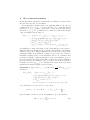
Given π and U (a), the symbolic backward reachability procedure iteratively
computes the set of backward
reachable states BR(a) as follows. Preliminarily,
W
let us put τ (a, a0 ) := h Lh (a, a0 ) ∨ E(a, a0 ); define also (for n ≥ 0) the n-preimage of a formula K(a) as
P re0 (τ, K) := K and P ren+1 (τ, K) := P re(τ, P ren (τ, K)),
where P re(τ, K) := ∃a0 .(τ (a, a0 ) ∧ K(a0 )). Intuitively, P ren (τ, U ) describes the
set of backward reachable states in n ≥ 0 steps. At the n-th iteration,
the backWn
ward reachability procedure computes the formula BRn (τ, U ) := i=0 P rei (τ, U )
representing the set of states which are backward reachable from the states in
U with at most n steps. While computing BRn (τ, U ), the procedure also checks
whether the system is unsafe by establishing if the formula I ∧ P ren (τ, U ) is
satisfiable modulo PTS (safety test) or whether a fix-point has been reached by
checking if (BRn (τ, U ) → BRn−1 (τ, U )) is PTS-valid or, equivalently, if the formula BRn (τ, U ) ∧ ¬BRn−1 (τ, U ) is PTS-unsatisfiable (fix-point test). If a safety
test is positive, the procedure returns UNSAFE; if this does not happen and a
fixed point is reached, the procedure returns SAFE.
The essential requirement in order to mechanize the procedure (which might
be non-terminating for various known general reasons) is the closure of ∃I formulae under preimage computation. In this way, in fact, a formula in the
sequence BR0 , BR1 ..., is an ∃I -formula and we need to check the satisfiability of
conjunctions of ∃I - and ∀I -formulae, which is decidable by using a general result
in [10]. Let K be an ∃I formula; while it is easy to show that P re(L, K) is equivalent to an ∃I -formula for any location transition L, it is unfortunately impossible
to prove it for P re(E, K). Although the existential variable ε can be eliminated
by using a standard quantifier-elimination procedure for Linear Real arithmetic,
the main difficulty is posed by the universal guard in (2), namely ∀j.φG (j, a[j], ).
In fact, it is known (see, e.g., [2]) that universal conditions are difficult to analyze automatically and require approximation techniques. In mcmt, the system
is approximated by using the stopping failures model [16] (similar to the “approximate model” of [1, 2]). According to this model, processes can crash at any
time and crashed processes remain so. In this way, the approximated system admits more runs than the original one and thus satisfies fewer safety properties.
As a consequence, if the approximated system enjoys a safety property, then we
are entitled to conclude that also the original system does so. In fact, establishing a safety property for the approximate system means that the system enjoys
that property in a “fault-tolerant way”, i.e., even in presence of failures. This
will be the case for all safety properties considered in this paper and also for
the deadlock freedom properties (modulo some provisoes discussed in Section 6
below). For a detailed description of how mcmt implements the stopping failures
model and for information on how to check whether an unsafety trace applies
to the original system, the reader is pointed to [4] (again, all unsafety traces
found in the experiments of this paper can be proved to apply to the original
version of the system without failures). We just point out that after moving to
the stopping failures model the desired closure property of ∃I -formulae under
preimages holds.
4
The Lynch-Shavit Algorithm
Lynch and Shavit [15] develop a time-based algorithm for mutual exclusion by
combining two other algorithms for mutual exclusion: a Lamport style asynchronous algorithm (see, e.g., [16]) and the well-known Fischer’s timed mutual
exclusion algorithm. The three algorithms presented in [15] consist of a finite
(but unknown) number n of identical processes running concurrently. Each process is composed of four regions of code:
Process i:
– remainder: the region of code not concerned with
the access to critical resources;
repeat forever
– trying: the region of code where the process tries
remainder region
to acquire access to the critical region;
trying region
– critical: the region of code with exclusive access;
critical region
– exit: the region of code where the process exits
exit region
from the critical region.
end repeat
Algorithm 1
Algorithm 2
Algorithm 3
x, y: shared registers
initially y = 0
x: shared register, initially 0
delay: positive integer constant
x, y: shared registers initially 0
delay: positive integer constant
repeat forever
0b: remainder exiti
L: x := i;
1: if y 6= 0 then goto L;
2: y := 1;
3: if x 6= i then goto L;
4a: critical entryi
4b: critical exiti
5: y := 0;
0a: remainder entryi
end repeat
repeat forever
0b: remainder exiti
L: if x 6= 0 then goto L;
1: x := i;
2: pause(delay);
3: if x 6= i then goto L;
4a: critical entryi
4b: critical exiti
5: x := 0;
0a: remainder entryi
end repeat
repeat forever
0b: remainder exiti
L: if x 6= 0 then goto L;
1: x := i;
2: pause(delay);
3: if x 6= i then goto L;
% Start of Critical Region
4: if y 6= 0 then goto L;
5: y := 1;
6: if x 6= i then goto L;
7a: critical entryi
7b: critical exiti
8: y := 0;
% End of Critical Region
9: x := 0;
0a: remainder entryi
end repeat
(1)
(2)
(3)
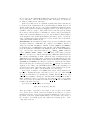
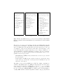
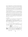
Fig. 1. The three Algorithms from [15] (code for process i): (1) Lamport’s Style Mutual
Exclusion; (2) Fisher’s Timed Mutual Exclusion; (3) Lynch-Shavit’s Combined Mutual
Exclusion.
The pseudo-code of a process i belonging to the three algorithms (taken verbatim
from [15]) is shown in Figure 1. Algorithm 1 is asynchronous while Algorithms 2
and 3 are timing-based: the time interval between successive steps of a process
i is assumed to range in some interval of time when i is in its trying or exit
region. The instruction pause(k) causes the process to delay by a number k − 1
of steps. Intuitively, pause(k) is equivalent to a sequence of k − 1 no-operations.
The idea is to choose values for time parameters in Algorithms 2 and 3 so as to
guarantee the two key properties:
– Mutual Exclusion (MEX): in any reachable state, at most one process is in
its critical region;
– Deadlock Freedom (DF): in any execution, if some process is in the trying
region, and no process is in the critical region, then eventually some process
enters the critical region.
Algorithm 1 enjoys property MEX but not DF. Two timing constraints are
crucial for Algorithms 2 and 3 [15]: (TC1) the time interval between successive
steps of a process i should be contained in [c1 , c2 ] (for 0 < c1 ≤ c2 < ∞) when
i is in its trying or exit region and (TC2) delay ≥ C = c2 /c1 where C is called
the time uncertainty. If (TC1)-(TC2) are satisfied, then both Algorithms 2,
3 satisfy MEX and DF, otherwise Algorithm 2 satisfies only property DF and
Algorithm 3 satisfies only property MEX. Since, ideally, timing-based algorithms
should guarantee mutual exclusion regardless of the timing constraints, in this
sense, Algorithm 3 is better designed than Algorithms 1 and 2.
Algorithm 1 can be formalized by a parameterized timed system
π1 := h∅, hpc, x, yi, {global(x), global(y), pc ∈ [1, 9]}, I, LT 1 , ∅i
where I := ∀i.pc[i] = 1 ∧ y = 0 and the integers 1, ..., 9 stands for the labels
0b, ..., 0a in the pseudo-code, LT 1 contains the location transition corresponding
to the various instructions in the pseudo-code. The tuple of parameters and the
set of time elapsing formulae of π1 are empty since time plays no role for an
asynchronous algorithm like the Algorithm 1.
Algorithm h ∈ {2, 3} is formalized by a parameterized timed system of the
form πh := hp, ah , Axh , Ih , LT h , TE h i, where
p := hC, F, Gi, a2 := hpc, pcclock , xi, a3 := hpc, pcclock , x, yi,
Ax2 := Ax ∪ {pc ∈ [1, 9]}, Ax3 := Ax ∪ {pc ∈ [1, 13], global(y)},
with Ax := {G ≥ F, F ≥ C, C ≥ 1, global(x), ∀i.pcclock [i] ≥ 0},
I2 := ∀i.pc[i] = 1 ∧ x = 0, I3 := ∀i.pc[i] = 1 ∧ x = 0 ∧ y = 0 ,
the location transition formulae in LT h are derived from the pseudo-code as
for Algorithm 1, the time elapsing formulae in TE h is of the form (2), and the
matrix φG of the universal guard is a conjunction of formulae of the form
pc[j] = q → pcclock [j] + ε ≤ Bq
(3)
saying that the location q has a bound Bq that cannot be violated if pcclock [j] is
updated to pcclock [j] + ε. (Recall that transitions of the form (1) should have set
the special clock variable pcclock [j] to 0 as soon as the process j enters location q.)
Two clarifications about the role of the parameters C, F , and G are mandatory
(the full formalization of Algorithm 2 is reported in Appendix B).
First observe that, without loss of generality, it is possible to assume c1 = 1: in
this way we will be able to use only Linear Arithmetic constraints, as prescribed
by the definition of parameterized timed system of Section 2. Thus we have
C = c2 /c1 = c2 . Because of the timing constraint (TC1), a process is forced
to remain in a location belonging to the trying or exit regions for at least 1
and at most C time units. This is encoded in πh (for h ∈ {2, 3}) with the two
following conditions (i)-(ii). Condition (i ) adds pcclock [i] ≥ 1 to the guards of
those location transition formulae that modify a control location inside the trying
or the exit regions. Condition (ii ) adds a conjuct of the form (3) to the universal
guard of the time elapsing formulae with Bq set to C, for each location inside
the trying or exit regions; the only exception is for the location corresponding
to the pause instruction, i.e., line 2 in the pseudo-code of Algorithms 2 and 3.
The second clarification is about the absence of the parameter delay and the
presence of the parameters F and G that do not occur in the pseudo-code of
Algorithms 2 and 3. The idea is to replace the obvious Non-Linear Arithmetic
constraint in the formulae of πh (for h ∈ {2, 3}) modelling pause(delay) with a
linear one involving F and G. In fact, the naive encoding of pause(delay) would
require the use of the non-linear term delay ∗ C to count the the number of
nullary operations that the process should wait before continuing its computations. Fortunately, as observed in [15], the key property of pause(delay) is that
its duration is greater than the time uncertainty C. Thus, the two additional
parameters F and G are used to model the minimum and maximum time span
that a process can spend inside pause(delay). In this way, the time constraint
(TC2) is encoded in πh (for h ∈ {2, 3}) by adding (i ) the condition pcclock [i] ≥ F
to the guard of the transition location in LT h modifying the control location q
and (ii ) a conjunct of the form (3) in the universal guard of the time elapsing
formulae in TE h with Bq set to G, where q is the control location associated to
the pause instruction (i.e., line 2 in the pseudo-code of Algorithms 2 and 3).
5
Automated Verification of Mutual Exclusion
We begin by reporting the results of our experiments on verifying the mutual
exclusion and other safety properties of the three algorithms. All the specification
files and scripts used in our experiments can be downloaded from the web page
http://www.oprover.org/mcmt_lynch_shavit.html.
Protocol
Lamport
Property
MEX
MEX
Fischer
MEX
MEX + I1
MEX
Lynch-Shavit MEX
MEX abstr.
Result Time (s)
safe
0.04
safe
2.64
unsafe
3.73
safe
(0.02 + 0.17) 0.19
safe
24.39
safe
353.91
safe
8.56
Notes
T. c. specified
T. c. not specified
Invariant added
T. c. specified
T. c. not specified
Uses mcmt’s abstraction
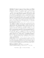
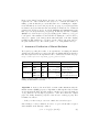
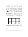
Table 1. Mutual exclusion experiments. Experiments were run on an Intel i7 2.70 GHz
running Ubuntu Linux 11.10 32-bits.
Algorithm 1. As it is clear from Table 1, mcmt verifies instantaneously the
mutual exclusion (MEX) property of Algorithm 1. Although the related results
are not shown in the Table, the same applies to the three properties of Lemma 3.2
of [15], which are used as helper properties to derive theorems in the original
paper. We briefly discuss Property I3 because it is not a safety property. It is
formulated as follows:
– I3: If y = 1 then some process i is not inside the remainder region.
Since mcmt proceeds by refutation, in order to be proved, I3 should be negated
and formalized as the unsafety condition
y = 1 ∧ ∀i. (pc[i] ∈ {0a, 0b})
(4)
which is not an existential formula, i.e., it cannot be handled directly by mcmt.
However it is not difficult to build an existential formula whose negation implies
the safety property represented by the negation of (4). The idea is to add a
historical variable H that records the id of the process that set y to 1 last
(initially H = 0); we use H to replace (4) with the weaker statement
y = 1 ∧ ∃i. (i = H ∧ pc[i] ∈ {0a, 0b})
(5)
which corresponds to the invariant
– I3’: If y = 1 then the process H that set y = 1 last is not inside the remainder
region.
We shall implicitly use similar tricks to transform some other safety lemma
statements arising in our experiments.
Algorithm 2. As discussed in Section 4, mutual exclusion for Algorithm 2
depends on timing constraints. This is confirmed by mcmt, as reported in the
rows 2-3 of Table 1. Also, it appears that checking mutual exclusion with the
help of Lemma 4.1 (I1), as suggested by [15], yields a substantial performance
improvement, see row 4, MEX + I1 (in order to use a Lemma, mcmt first verifies
it and then adds it to the set of system axioms).
Algorithm 3. Algorithm 3 combines the previous two and guarantees both
mutual exclusion (even without timing constraints) and deadlock-freedom (with
timing constraints). In Table 1 we check with mcmt that Algorithm 3 has the
mutual exclusion property, even without timing constraints (rows 5-6). mcmt
implements only a rudimentary form of abstraction which might be used during
invariant search. Since mutual exclusion for Algorithm 3 does not depend on
timing information at all, one can try to ask the tool to abstract away any
timing information: with this proof strategy, mutual exclusion without timing
constraints is established much quicker (compare lines 7 and 6 from Table 1). We
just mention that it is possible to quickly check with mcmt also other lemmata
from [15], e.g., those that are used as ingredients for the proof of the deadlockfreedom property.
6
Automated Verification of Deadlock Freedom
Algorithms 2 and 3 have the deadlock freedom property: interestingly, time
bounds for waiting time are independent on the size of the network and can
be expressed as linear polynomials p(C, G) involving the parameters G and C.
This raises the possibility of verifying deadlock-freedom using mcmt, even if
mcmt can only accept safety problems. We first show how to do it with manual
intervention and then we fully automatize the whole procedure by synthesizing
both invariants and polynomial bounds.
6.1
Verification
We first suppose that we already know the linear polynomials giving the time
bounds (p(C, G) = 2 ∗ G + 5 ∗ C for Algorithm 2 and p(C, G) = 2 ∗ G + 9 ∗ C
for Algorithm 3); we just want to check that such bounds are correct by using
mcmt. Thus we want to check that “if some process is in the trying region, and
no process is in the critical region, then before p(C, G) time units have passed
some process enters the critical region”. The first idea is the following:
(i) we add an absolute clock absclock and a boolean flag k to the specification
(the Boolean flag k is permanently turned to true as soon as one process
reaches the critical region);
(ii) we initialize the system by putting absclock := 0, k := false, and by
saying that no process is in critical region and that the process having N
as an id is in the trying region (N is a new parameter of type INT subject
to the constraint N > 0);
(iii) we consider unsafe the states in which absclock > p(C, G) and k = false.
For various reasons, the above idea is not correct (indeed mcmt returns
UNSAFE if you implement it, even if the chosen bound p(C, G) is correct). We
need to identify these reasons and make the suitable adjustments to our plan.
The reason for a first adjustment is clear: mcmt adopts the stopping failures
model (due to the presence of universal quantifiers in transitions guards) and in
the stopping failures model deadlock freedom does not hold (as a trivial counterexample, consider the run in which a process i sets the shared register x to i
and then crashes, thus preventing any other process to access the critical region
forever). However, crashes can be tolerated without losing deadlock freedom,
provided some key actors do not crash: there is a limited (albeit sufficient) possibility to tell this to mcmt. Notice that, whenever mcmt adopts the stopping
failures models, it automatically relativizes quantifiers to non-crashed processes
(see [4] for details). Recall also that a process that crashes is crashed forever:
as a consequence, processes that are existentially quantified in the unsafety formula cannot be crashed. Thus, the proposal is to use as unsafety formula the
disjunction of the following three existential sentences:
∃i1 ∃i2 (i1 = N ∧ i1 6= i2 ∧ x = i2 ∧ k = false ∧ absclock > p(C, G))
(6)
∃i1 (i1 = N ∧ x = i1 ∧ k = false ∧ absclock > p(C, G))
(7)
∃i1 (i1 = N ∧ x = 0 ∧ k = false ∧ absclock > p(C, G))
(8)
In this way we are guaranteed that process N (i.e., the one who was trying to
access the critical region from the very beginning) does not get crashed and
that, in case an undesired state is reached, it will be reached either with an
uninitialized shared register or with the shared register set to the id of a non
crashed process. This is much weaker than saying that there are no crash failures
at all, but it is sufficient for our problems.
Still, mcmt gives UNSAFE and now comes the reason for our second adjustment: we need to constrain the initial states to be “reachable” states of our
Algorithms 2 and 3. The notion of “reachable state” needs not to be definable,
however we can overapproximate it by using suitable lemmata. This is in a sense
the strategy of [15]: suitable lemmata describing seemingly interesting properties
of the reachable states are invented, then they are formally proved and finally
they are used when proving the correctness of time bounds for deadlock freedom. In our experiments, we proposed two lemmata for Algorithm 2 and three
lemmata for Algorithm 3; such lemmata are checked by using mcmt itself (in a
total amount of time of 8.95 sec. for Algorithm 2 and 236.51 sec. for Algorithm
3) and then they are added as system axioms to the specification file of the time
bounds for deadlock-freedom (we shall see below how to automatically synthesize the lemmata). In other words, we try to prove that the deadlock-freedom
property and the related time bound for the access to the critical region apply to
all the states that satisfy the lemmata we found, independently on whether such
states are really reachable or not.
But now another problem arises: mcmt diverges. In fact, termination is not
guaranteed at all, because we are outside the scope of decidability results known
from the literature. However, the divergence source is limited and we can fruitfully apply a well-know model checking technique, namely acceleration (this will
be our third and last adjustment). The point is that the sequence of the two
transitions formed by line code L (for a fixed process i) and time elapsing can be
indefinitely applied: we need to insert a further transition modeling n executions
of this sequence for an arbitrary n. This is definable in the format accepted by
mcmt, details are shown in the Appendix A below. After this last adjustment,
mcmt is able to check the time bounds in 80.97 sec. and in 1374.38 sec. for
Algorithms 2 and 3, respectively.
6.2
Synthesis
The insertion of the accelerated transition is the only manual intervention that
is actually needed. In fact, both the lemmata used to overapproximate the set
of reachable states and the polynomial p(C, G) can be synthesized.
Invariant Synthesis. Suppose first the polynomial p(C, G) is fixed; let us run
mcmt on our Algorithm 2 (or 3), with the unsafety formula given by the disjunction of (6)-(8) and with the initial formula I(a, absclock , k) given by the
statement suggested in 6.1(ii), namely
absclock = 0 ∧ k = false ∧ ∀i (i = N → pc[i] ∈ T ry)
(9)
(here pc[i] ∈ T ry) abbreviates a disjunction saying that pc[i] is equal to one
of the locations of the trying region). The tool returns UNSAFE by producing
an ∃I -formula P := ∃iφ(i, a[i], k, absclock , N ), which means that that during the
safety check the formula
∃iφ(i, a[i], k, absclock , N ) ∧ I(a, absclock , k)
(10)
is reported to be PTS-satisfiable. Now notice that (6)-(8) all contain the conjunct i1 = N , which is not modified during the calculus of preimages, thus
φ(i, a[i], k, absclock , N ) is of the kind i1 = N ∧ ψ(i1 , j, a[i1 ], a[j], k, absclock , N ).
Taking into consideration (9) and the instantiation algorithm for PTS-satisfiability given in [10], the PTS-unsatisfiability of (10) means that the formula
^
(i = i1 → pc[i] ∈ T ry)
(11)
ψ(i1 , j, a[i1 ], a[j], false, 0, i1 ) ∧
i∈i1 ,j
is not PTS-satisfiable. The idea is to check whether the negation of this formula
can be used as a lemma, i.e., if it is an overapproximation of the set of reachable
states. To check this, it is sufficient to run mcmt on the problem having the
standard initialization of Algorithm 2 (resp. 3) and having precisely (11) as
an unsafe formula. If the tool returns UNSAFE, then the bound p(C, G) is not
correct, because composing the two traces leading to the unsafe sets of states,
we have a counterexample showing that the time bound can be violated. If
the tool returns SAFE, then we can repeat our attempt of verifying the time
bound, but in the new run we add the negation of (11) as a system axiom. As a
consequence, the formula (10) is not satisfiable anymore and the tool won’t exit
if ∃iφ(i, a[i], k, absclock , N ) is produced. Of course, the tool may still produce an
UNSAFE outcome, in which case the procedure must be repeated. In the end,
provided divergence does not arise, the tool either synthesizes enough lemmata
and certifies that the time bound is correct or it finds a counterexample for it.
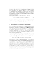
Time Bounds Synthesis. The above procedure works independently on the
fact whether the time bound we suggest to the tool is correct or not, thus it is
possible to use it in order to get the optimal polynomial p(C, G). In fact, what
we are looking for is a linear polynomial α ∗ C + β ∗ G with positive integers
coefficients: we can just begin with α = 1, β = 1 and then increment the values
with a dichotomic search as soon as we get a counterexample. The statistics of
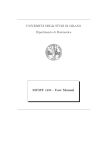
our experiments, for values close to the optimum, are reported in Table 2.
Protocol
α, β Bound Holds Iterations Time (s)
2, 2
NO
1
62.06
2, 4
NO
5
110.68
Fischer
2, 5
YES
8
155.56
2, 6
YES
6
130.69
2, 10
YES
3
51.25
2, 2
NO
1
224.74
2, 8
NO
11
5764.42
Lynch-Shavit 2, 9
YES
16
27995.78
2, 10
YES
10
6935.91
2, 14
YES
3
974.06
Table 2. Time bounds synthesis. The table reports the attempts of checking a polynome with given α and β coefficients. The optimal values found (2 5 for Fischer and 2
9 for Lynch-Shavit) coincide with the known theoretical optimal bounds. Experiments
were run on an Intel i7 2.70 GHz running Ubuntu Linux 11.10 32-bits.
7
Discussion
We have described how mutual exclusion and deadlock-freedom of a class of
timing-based algorithms can be specified and automatically verified by the model
checker mcmt. We have highlighted how two kinds of being parametric are supported by our framework, namely with respect to the number of processes in the
system and the symbolic constants in the timing constraints. We have illustrated
our approach on the Lynch-Shavit algorithm.
To the best of our knowledge, it is the first time that a formal and automatic
analysis of this algorithms is performed. Key to the automated verification of
deadlock-freedom is the use of acceleration (to avoid non-termination) combined
with the automated synthesis of invariants to be used as lemmata in the main
proof (to realize a fully automated analysis procedure).
Related Work. To the best of our knowledge, analysis techniques for the verification of parameterized systems seldom consider the two dimensions of the
parameters as we do here. For example, [9, 17] consider only finite-state processes while [3] presents a method for the verification of a parametric number
of timed automata with real-valued clocks. Our notion of parameterized timed
systems is strictly more general than that in [9, 17] by allowing for arithmetic
variables and that of [3] by allowing for location invariants (see Section 2) in
timed transitions.
There is also a substantial body of work on the analysis of safety properties
for parameterized systems with an arbitrary number of processes operating on
bounded and unbounded variables, see, e.g., [13, 14, 20]. These methods are not
targeted to the verification of timing-based algorithms and consider only safety
properties whereas we also tackle the problem of verifying a restricted class of
liveness properties. The approach in [8] uses SMT techniques to verify systems
with several dimensions in the parameters but it only supports invariant checking
or bounded model checking.
In [5, 7, 19], SAL is used to model check several timed systems. In contrast
to our approach that is fully automatic, these approaches require some amount
of user interaction, which is reasonable given the large size of some of the systems (especially those in [5]). The model checker Uppaal [22] is capable of automatically checking both safety and liveness of timed automata without timing
parameters. An extension of Uppaal described in [12] is capable of synthesizing
linear parameter constraints for the correctness of the timed automata. Both of
these approaches are not parametric in the number of processes. Our approach
is parametric both in the number of processes and in the time constraints but
does not attempt to perform the synthesis of linear arithmetic constraints although, in principle, this would possible and we leave it to future work. Here, we
focus on the automated synthesis of invariants to be used as lemmata in proving
deadlock-freedom.
In our previous work on mcmt [6,10], we have only considered safety properties of parametric systems while here we verify also a restricted class of liveness
properties. Furthermore, the analysis presented here is much more fine-grained
than that in [6], because, for instance, specific time interval bounds are considered for each step of the protocols and not just for few relevant locations. This
additional precision in the formalization significantly increases the difficulty of
the verification tasks.
References
1. P. A. Abdulla, G. Delzanno, N. B. Henda, and A. Rezine. Regular model checking
without transducers. In TACAS, volume 4424 of LNCS, pages 721–736, 2007.
2. P. A. Abdulla, G. Delzanno, and A. Rezine. Parameterized verification of infinitestate processes with global conditions. In CAV, LNCS, pages 145–157, 2007.
3. Parosh Aziz Abdulla and Bengt Jonsson. Model checking of systems with many
identical timed processes. Theoretical Computer Science, pages 241–264, 2003.
4. F. Alberti, S. Ghilardi, E. Pagani, S. Ranise, and G. P. Rossi. Universal Guards,
Relativization of Quantifiers, and Failure Models in Model Checking Modulo Theories. JSAT, 8:29–61, 2012. Available at http://jsat.ewi.tudelft.nl/
content/volume8/JSAT8_2_Alberti.pdf.
5. G. Brown and L. Pike. Easy Parameterized Verification of Biphase and 8N1 Protocols. In TACAS, pages 58–72, 2006.
6. A. Carioni, S. Ghilardi, and S. Ranise. MCMT in the Land of Parametrized Timed
Automata. In Proc. of VERIFY 10, 2010.
7. B. Dutertre and M. Sorea. Timed systems in sal. Technical Report SRI-SDL-04-03,
SRI International, Menlo Park, CA, 2004.
8. J. Faber, C. Ihlemann, S. Jacobs, and V. Sofronie-Stokkermans. Automatic Verification of Parametric Specifications with Complex Topologies. In IFM, volume
6396 of LNCS, pages 152–167, 2010.
9. Yi Fang, Nir Piterman, Amir Pnueli, and Lenore D. Zuck. Liveness with invisible
ranking. Software Tools for Technology, 8(3):261–279, 2006.
10. S. Ghilardi and S. Ranise.
Backward reachability of array-based systems
by SMT-solving: termination and invariant synthesis.
LMCS, 6(4), 2010.
Available at http://www.lmcs-online.org/ojs/viewarticle.php?id=
694&layout=abstract.
11. S. Ghilardi and S. Ranise. MCMT: A Model Checker Modulo Theories. In Proc.
of IJCAR 2010, LNCS, 2010.
12. T. Hune, J. Romijn, M. Stoelinga, and F. W. Vaandrager. Linear Parametric
Model-Checking of Timed Automata. In TACAS, pages 189–203, 2001.
13. S. Krstic. Parameterized system verification with guard strengthening and parameter abstraction. In AVIS, 2005.
14. S. K. Lahiri and R. E. Bryant. Predicate abstraction with indexed predicates.
ACM Transactions on Computational Logic (TOCL), 9(1), 2007.
15. N. A. Lynch and N. Shavit. Timing-based mutual exclusion. In Proc. of IEEE
Real-Time Systems Symposium, pages 2–11, 1992.
16. Nancy A. Lynch. Distributed Algorithms. Morgan Kaufmann, 1996.
17. A. Pnueli, S. Ruath, and L. D. Zuck. Automatic deductive verification with invisible invariants. In Proc. of TACAS 2001, volume 2031 of LNCS, 2001.
18. S. Ranise and C. Tinelli. The SMT-LIB Standard: Version 1.2. Technical report,
2006. Available at http://www.SMT-LIB.org/papers.
19. W. Steiner and B. Dutertre. Automated Formal Verification of the TTEthernet
Synchronization Quality. In Proc. of the NASA Formal Methods Symposium, 2011.
20. M. Talupur and M. Tuttle. Going with the flow: Parameterized verification using
message flows. In Proc. of FMCAD 08, page ??, 2008.
21. mcmt web site. http://www.dsi.unimi.it/˜ghilardi/mcmt/.
22. Uppaal. http://www.uppaal.com.
A
The accelerated transition
In this Appendix we discuss the formal details concerning the accelerated transitions we introduced in our experiments.
Let us analyze the following sequence of steps (in Algorithm 2 or 3): a process
i with local clock pcclock [i] ≥ c1 executes the line code L, then time has an
increment by ε ∈ [c1 , c2 ], then i executes line L again, then time has another
increment ε ∈ [c1 , c2 ], etc. etc. If this is done n times, the result is the following
composed transition (let us call it τn )
Vn
∃i ∃ε1 · · · εn
(pc[i] = L ∧ pcclock [i] ≥ c1 ∧
k=1 c1 ≤ εk ≤ c2 ∧
P
∧ ∀j 6= i (pc[j] 6∈ RM ∪ {2} → pcclock [j] + k εk ≤ c2 ) ∧
P
∧ ∀j (pc[j] = 2 → pcclock [j] + k εk ≤ G) ∧
P
∧ abs0clock = absclock + k εk ∧
P
∧ pc0clock = λj.(if j = i then 0 else pcclock [j] + k εk ))
(for simplicity, we omitted the updates of the arrays, like the location array pc,
which are updated identically; we also generically called RM the locations in the
remainder region). Now, during mcmt runs for our deadlock freedom problems,
existential formulae K such that the formulae P re(τn , K) are more and more
informative (varying n) arise, so that backward search does not terminate.
W The
acceleration technique consists in inserting a single extra transition n≥M τn
(for some M ) in the specification file: if this operation succeeds, the termination
problems caused by theWpreimages of the τn would be solved.The key question
is whether transitions n≥M τn are definable in the format allowed for mcmt
transitions. An answer is supplied by the following
W
1
. Then n≥M τn is
Proposition 1. Suppose that c2 > c1 and that M ≥ c2c−c
1
equivalent to
∃i ∃ε ≥ M ∗ c1
(pc[i] = L ∧ pcclock [i] ≥ c1 ∧
∧ ∀j 6= i (pc[j] 6∈ RM ∪ {2} → pcclock [j] + ε ≤ c2 ) ∧
∧ ∀j (pc[j] = 2 → pcclock [j] + ε ≤ G) ∧
∧ abs0clock = absclock + ε ∧
∧ pc0clock = λj.(if j = i then 0 else pcclock [j] + ε))
Proof. All what we need is to show for every ε that
ε ≥ M ∗ c1
⇔
∃n ≥ M ∃ε1 , . . . , εn ∈ [c1 , c2 ] s.t. ε =
n
X
εk .
k=1
Since the right-to-left side is obvious, it is sufficient to prove the inclusion
[
[M ∗ c1 , ∞) ⊆
[n ∗ c1 , n ∗ c2 ]
(12)
n≥M
(in fact, if (12) holds, for any ε ≥ M ∗ c1 there is some n ≥ M such that n ∗ c1 ≤
ε ≤ n ∗ c2 and we can take ε1 = · · · = εn := ε/n). To show (12) it is sufficient to
prove that for ñ ≥ M the intervals [ñ ∗ c1 , ñ ∗ c2 ] and [(ñ + 1) ∗ c1 , (ñ + 1) ∗ c2 ]
overlap, i.e. are such that (ñ + 1) ∗ c1 ∈ [ñ ∗ c1 , ñ ∗ c2 ]. However (since c1 is
positive) (ñ + 1) ∗ c1 ∈ [ñ ∗ c1 , ñ ∗ c2 ] is equivalent to (ñ + 1) ∗ c1 ≤ ñ ∗ c2 and to
c1 ≤ ñ ∗ (c2 − c1 ), thus any ñ ≥ M has this property.
a
In our situation, we have c1 = 1 and c2 = C; thus Proposition 1 applies for
C > 1 and M ≥ 1/(C −1). If we put M := d1/(C −1)e, the above Proposition
indicates an accelerated transition solving our divergence problem (we say that
a transition is accelerated if, after adding it to the current set of transitions, the
new runs that arise are obtained from old runs by replacing a sequence of steps
1
e is
by a single new step). Still there is the problem that the atom ε ≥ d C−1
not linear (hence it cannot be handled by the backhand SMT solver of mcmt);
in addition, the case C = 1 is not covered. In our experiments we used the
transition
∃i ∃ε ≥ 1
(pc[i] = L ∧ pcclock [i] ≥ 1 ∧
∧ ∀j 6= i (pc[j] 6∈ RM ∪ {2} → pcclock [j] + ε ≤ C) ∧
∧ ∀j (pc[j] = 2 → pcclock [j] + ε ≤ G) ∧
∧ abs0clock = absclock + ε ∧
∧ pc0clock = λj.(if j = i then 0 else pcclock [j] + ε))
By the above Proposition, this transition is an accelerated transition in case
1
1 ≥ C−1
and C > 1, that is only in case C ≥ 2 (otherwise it may introduce
spurious runs). However, since we luckily succeeded in proving time bounds for
deadlock freedom in this way, these time bounds apply to the general case too
(trivially, if they apply to honest and possibly spurious runs, they in particular
apply to all honest runs). Notice also that whenever we check tightness of these
time bounds, mcmt returns UNSAFE, hence it does not diverge and we do not
need the accelerated transition at all.
B
The formalization of Algorithm 2
We report the full formalization of Algorithm 2 (the Fischer protocol) as a
parameterized timed system π := hp, a, Ax, I, LT , TE i. We have
p := hC, F, Gi,
a := hpc, pcclock , xi,
Ax := {G ≥ F, F ≥ C, C ≥ 1, pc ∈ [1, 9], global(x), ∀i.pcclock [i] ≥ 0},
I := ∀i.pc[i] = 1 ∧ x = 0.
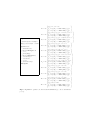
The location transition formulae in LT are derived from the pseudo-code of
Algorithm 2 and are reported in Figure 2 (the names of the locations from
Figure 1 have been renamed progressively as 1, . . . , 9 to make comparison with
location transitions easier).
The time elapsing transition TE is specified as follows:
0
x = x ∧ pc0 = pc ∧ ∀j φG ∧
∃ε > 0.
pc0c = λj.(pcc [j] + ε)
where φG is the conjunction of the following two conditions
pc[j] 6= 1 ∧ pc[j] 6= 4 ∧ pc[j] 6= 6 ∧ pc[j] 6= 9 → pcc [j] + ε ≤ C
pc[j] = 4 → pcc [j] + ε ≤ G
(the two conditions give upper bounds for the time a process can stay in a
location from the trying or exit region).

pc[i] = 1 ∧ x0 = x∧
0
∃i.  pc = λj. (if j = i then 2 else pc[j]) ∧ 
pc0c = λj. (if j = i then 0 else pcc [j])


pc[i] = 2 ∧ pcc [i] ≥ 1 ∧ x = 0 ∧ x0 = x ∧
0

∃i.  pc = λj. (if j = i then 3 else pc[j]) ∧
pc0c = λj. (if j = i then 0 else pcc [j])


pc[i] = 2 ∧ pcc [i] ≥ 1 ∧ x 6= 0 ∧ x0 = x ∧

∃i.  pc0 = λj. (if j = i then 2 else pc[j]) ∧
pc0c = λj. (if j = i then 0 else pcc [j])


pc[i] = 3 ∧ pcc [i] ≥ 1 ∧ x0 = i ∧
∃i.  pc0 = λj. (if j = i then 4 else pc[j]) ∧ 
pc0c = λj. (if j = i then 0 else pcc [j])


pc[i] = 4 ∧ pcc [i] ≥ F ∧ x0 = x ∧
0
∃i.  pc = λj. (if j = i then 5 else pc[j]) ∧ 
pc0c = λj. (if j = i then 0 else pcc [j])


pc[i] = 5 ∧ pcc [i] ≥ 1 ∧ x = i ∧ x0 = x∧
0

∃i.  pc = λj. (if j = i then 6 else pc[j]) ∧
pc0c = λj. (if j = i then 0 else pcc [j])


pc[i] = 5 ∧ pcc [i] ≥ 1 ∧ x 6= i ∧ x0 = x∧
0

∃i.  pc = λj. (if j = i then 2 else pc[j]) ∧
pc0c = λj. (if j = i then 0 else pcc [j])


pc[i] = 6 ∧ pcc [i] ≥ 1 ∧ x0 = x∧
∃i.  pc0 = λj. (if j = i then 7 else pc[j]) ∧ 
pc0c = λj. (if j = i then 0 else pcc [j])


pc[i] = 7 ∧ pcc [i] ≥ 1 ∧ x0 = x∧
∃i.  pc0 = λj. (if j = i then 8 else pc[j]) ∧ 
pc0c = λj. (if j = i then 0 else pcc [j])


pc[i] = 8 ∧ pcc [i] ≥ 1 ∧ x0 = 0∧
0
∃i.  pc = λj. (if j = i then 9 else pc[j]) ∧ 
pc0c = λj. (if j = i then 0 else pcc [j])


pc[i] = 9 ∧ x0 = 0∧
0
∃i.  pc = λj. (if j = i then 1 else pc[j]) ∧ 
pc0c = λj. (if j = i then 0 else pcc [j])

L1 :=
L2 :=
Algorithm 2
L3 :=
x: shared register, initially 0
delay: positive integer constant
L4 :=
repeat forever
1: remainder exiti
2: if x 6= 0 then goto L;
3: x := i;
4: pause(delay);
5: if x 6= i then goto L;
6: critical entryi
7: critical exiti
8: x := 0;
9: remainder entryi
end repeat
L5 :=
L6 :=
L7 :=
L8 :=
L9 :=
L10 :=
L11 :=
Fig. 2. Algorithm 2: pseudo-code and location transitions (pcc above abbreviates
pcclock ).