Download Thin Film Deposition & Vacuum Technology

Thin Film Deposition
& Vacuum Technology
THIN FILM DEPOSITION & VACUUM TECHNOLOGY
By
Stefan Cannon Lofgran
A senior thesis submitted to the faculty of
Brigham Young University–Idaho
in partial fulfillment of the requirements for the degree of
Bachelor of Science
Department of Physics
Brigham Young University–Idaho
April 2013
c Stefan Lofgran
2013 All Rights Reserved
Brigham Young University–Idaho
Department Approval
of a senior thesis submitted by
Stefan Cannon Lofgran
This thesis has been reviewed by the research committee, senior thesis coordinator and department chair and has been found to be satisfactory.
Date
David Oliphant, Advisor
Date
Ryan Nielson, Committee Member
Date
Stephen McNeil, Senior Thesis Coordinator
ABSTRACT
THIN FILM DEPOSITION & VACUUM TECHNOLOGY
Stefan Cannon Lofgran
Department of Physics
Bachelor of Science
The study and development of thin films via physical vapor deposition has
played a significant role in the development of optical coatings, semiconductors, and solar cells. Closely related to the study of thin films is the development of vacuum technology and systems capable of reaching pressures
suitable for growing uniform films at reasonable deposition rates. This paper
explores the method of physical vapor deposition known as thermal evaporation via resistive or Joule heating as a means for growing thin aluminum
(Al) films on a mineral glass substrate. Methods for measuring thickness are
also discussed and investigated in an attempt to determine the experimentally produced film thickness. A detailed explanation of the development and
operation of the vacuum system in which the Al films were grown is given as
well as future improvements that could be made.
iii
ACKNOWLEDGEMENTS
To my loving wife & family who have supported me the
whole way, and to David Oliphant who has guided me on
this project.
iv
Table of Contents
Abstract . . . . . .
Acknowledgements
List of Figures . . .
List of Tables . . .
.
.
.
.
.
.
.
.
.
.
.
.
.
.
.
.
.
.
.
.
.
.
.
.
.
.
.
.
.
.
.
.
.
.
.
.
.
.
.
.
.
.
.
.
.
.
.
.
.
.
.
.
.
.
.
.
.
.
.
.
.
.
.
.
.
.
.
.
.
.
.
.
.
.
.
.
.
.
.
.
.
.
.
.
.
.
.
.
.
.
.
.
.
.
.
.
.
.
.
.
.
.
.
.
.
.
.
.
.
.
.
.
.
.
.
.
.
.
.
.
Page
.
iii
.
iv
. vii
. viii
1 Introduction
1.1 A Brief History of Thin Film &
Vacuum Technology . . . . . . . . . . . . . . . . . . . . . . . . . . . .
1.2 Review of Theory . . . . . . . . . . . . . . . . . . . . . . . . . . . . .
2 Experimental Design & Setup
2.1 Vacuum System Design . . . . . . . . . . . . . . . . . . . . .
2.1.1 Recent Developments . . . . . . . . . . . . . . . . . .
2.1.2 Using a Viton Gasket . . . . . . . . . . . . . . . . . .
2.1.3 Vacuum Conditioning . . . . . . . . . . . . . . . . . .
2.2 Deposition System Design . . . . . . . . . . . . . . . . . . .
2.2.1 The Original Experiment . . . . . . . . . . . . . . . .
2.2.2 New Crucibles & Improved Temperature Calculations
2.2.3 Power Supplies & Feedthroughs . . . . . . . . . . . .
2.2.4 Substrate Holder Design . . . . . . . . . . . . . . . .
3 Procedures & Documentation
3.1 Equipment Documentation . . . . . .
3.1.1 Silicon Heating Tape . . . . .
3.1.2 Type C Thermocouple . . . .
3.1.3 Quartz Crystal Microbalance
3.1.4 Residual Gas Analyzer . . . .
3.1.5 Crucibles, Baskets, & Boats .
v
.
.
.
.
.
.
.
.
.
.
.
.
.
.
.
.
.
.
.
.
.
.
.
.
.
.
.
.
.
.
.
.
.
.
.
.
.
.
.
.
.
.
.
.
.
.
.
.
.
.
.
.
.
.
.
.
.
.
.
.
.
.
.
.
.
.
.
.
.
.
.
.
.
.
.
.
.
.
.
.
.
.
.
.
.
.
.
.
.
.
.
.
.
.
.
.
.
.
.
.
.
.
.
.
.
.
.
.
.
.
.
.
.
.
.
.
.
.
.
.
.
.
.
.
.
.
.
.
.
.
.
.
.
.
.
.
.
.
1
1
4
.
.
.
.
.
.
.
.
.
9
9
9
10
12
14
14
15
17
18
.
.
.
.
.
.
21
21
21
22
23
24
25
.
.
.
.
.
25
26
26
27
28
4 Thin Film Deposition Rates
4.1 Initial Rate Calculations . . . . . . . . . . . . . . . . . . . . . . . . .
4.2 Effects of Slide Outgassing . . . . . . . . . . . . . . . . . . . . . . . .
29
29
31
5 Future Experiments & Summary
5.1 Improving Film Quality . . . . . . . . . . . . . . . . . . . . . . . . .
5.2 Improved Deposition Rates . . . . . . . . . . . . . . . . . . . . . . . .
35
35
36
Bibliography
38
Appendix A
40
Appendix B
42
Appendix C
45
Appendix D
49
Appendix E
50
Appendix F
53
3.2
3.3
3.1.6 Power Supplies . . . . . .
Vacuum Procedures . . . . . . . .
3.2.1 Pumping to Low Vacuum
3.2.2 Pumping to High Vacuum
Deposition Procedure . . . . . . .
vi
.
.
.
.
.
.
.
.
.
.
.
.
.
.
.
.
.
.
.
.
.
.
.
.
.
.
.
.
.
.
.
.
.
.
.
.
.
.
.
.
.
.
.
.
.
.
.
.
.
.
.
.
.
.
.
.
.
.
.
.
.
.
.
.
.
.
.
.
.
.
.
.
.
.
.
.
.
.
.
.
.
.
.
.
.
.
.
.
.
.
.
.
.
.
.
List of Figures
1.1
1.2
1.3
RGA cracking patterns . . . . . . . . . . . . . . . . . . . . . . . . . .
Langmuire-Knudsen angle dependence . . . . . . . . . . . . . . . . .
Initial deposition system configuration . . . . . . . . . . . . . . . . .
2.1
2.2
2.3
2.4
2.5
2.6
2.7
2.8
2.9
2.10
BYU-Idaho Vacuum system . . .
25” OD CF Flange . . . . . . . .
O-ring over compression failure .
RGA P vs T graph . . . . . . . .
Various boats and baskets [1] . .
Broken tungsten baskets . . . . .
Broken quartz crucibles . . . . . .
New crucible holder configuration
Old crucible configuration . . . .
Substrate holder design . . . . . .
.
.
.
.
.
.
.
.
.
.
10
11
12
14
15
16
17
18
19
20
3.1
3.2
Quartz Crystal Microbalance Positioning . . . . . . . . . . . . . . . .
Crucible & basket combination . . . . . . . . . . . . . . . . . . . . .
24
25
4.1
4.2
4.3
Filmed slide projection . . . . . . . . . . . . . . . . . . . . . . . . . .
Average change in slide mass over time . . . . . . . . . . . . . . . . .
Change in slide mass between consecutive days . . . . . . . . . . . . .
30
33
34
vii
.
.
.
.
.
.
.
.
.
.
.
.
.
.
.
.
.
.
.
.
.
.
.
.
.
.
.
.
.
.
.
.
.
.
.
.
.
.
.
.
.
.
.
.
.
.
.
.
.
.
.
.
.
.
.
.
.
.
.
.
.
.
.
.
.
.
.
.
.
.
.
.
.
.
.
.
.
.
.
.
.
.
.
.
.
.
.
.
.
.
.
.
.
.
.
.
.
.
.
.
.
.
.
.
.
.
.
.
.
.
.
.
.
.
.
.
.
.
.
.
.
.
.
.
.
.
.
.
.
.
.
.
.
.
.
.
.
.
.
.
.
.
.
.
.
.
.
.
.
.
.
.
.
.
.
.
.
.
.
.
.
.
.
.
.
.
.
.
.
.
.
.
.
.
.
.
.
.
.
.
.
.
.
.
.
.
.
.
.
.
5
6
7
List of Tables
1.1
Vacuum quality pressure ranges . . . . . . . . . . . . . . . . . . . . .
2
3.1
3.2
3.3
Silicon Heat Tape Specifications . . . . . . . . . . . . . . . . . . . . .
Type C thermocouple specifications . . . . . . . . . . . . . . . . . . .
Genesys 60-12.5 power supply details . . . . . . . . . . . . . . . . . .
22
23
26
viii
Chapter 1
Introduction
1.1
A Brief History of Thin Film &
Vacuum Technology
Vacuum technology is becoming increasingly important within physics due to its
several applications. The ideal vacuum is a space devoid of all particles. All vacuum
systems aren’t created equal, and like many things in physics actual vacuum
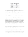
systems fall short of the ideal. The base pressure a system maintains determines the
quality of its vacuum. These levels aren’t strictly defined, but are generally
described as rough, low, medium, high, or ultra high (see Table 1.1). The most
obvious factors determining the type of vacuum achieved are the equipment used
and the system configuration. Before delving into the details of vacuum design and
its importance in developing thin films it will be beneficial to review a brief history
of how vacuum systems were first developed.
One of the first contributors to vacuum technology was Otto von Guericke. Von
Guericke developed the first vacuum pump sometime in the 1650’s[2]. With his
pump, he was able to study some of the most basic properties of vacuums. Von
Guericke believed that his pump pulled the air out of a container, which is actually
incorrect. Vacuum pumps cannot pull the gases out of a container rather they
1
Table 1.1: Vacuum quality pressure ranges
create a difference in pressure which causes the gas in the high-pressure area to
move to the low-pressure area. Essentially, a vacuum pump generates a vacuum by
creating pressure differences, which creates a flow of gas that exits the chamber at a
rate faster than the rate at which gas enters the chamber.
Aside from Von Guericke, there were several other contributors to what is now
considered modern vacuum technology. Many of these individuals lived before or
during the same time as Otto von Guericke. Evangelista Torricelli, the man who the
unit of pressure Torr is named after, was one of the first to recognize a sustained
vacuum while observing mercury in a long tube. He noted his discovery, but never
actually published his findings because he was more interested in mathematics.
Hendrik Lorentz, Blaise Pascal, Christiaan Huygens, and others all played crucial
roles in defining and developing the fundamental principles upon which modern
vacuum systems run.
Modern vacuum technology is constantly adapting to be used in a broader range
of applications in a plethora of disciplines within physics and engineering, such as
vacuum packaging, welding, and electron microscopes. Even though vacuum
technology has developed rapidly since the 1600’s, what most would define as
modern vacuum technology isn’t that old. Scientists and engineers developed most
of the technology that we use today during and after World War II. During the
2
period of development after World War II people began to revisit thin films and
explore the possibilities of their uses in industry, particularly in the semiconductor
industry.
One of the most important applications of vacuum systems is the development of
thin films. Physical vapor deposition (PVD) is just one method of producing thin
films. Michael Faraday pioneered the first PVD process in the early 1800’s [1].
Many sub processes fall under the description of PVD including electron beam,
sputtering, thermal, and plasma arc deposition methods. At BYU-Idaho the
method used to produce thin films is a thermal evaporative deposition. Thermal
evaporation deposition is the most basic method used to produce thin films. The
first use of the term PVD was used in C. F. Powell, J. H. Oxley, and J. M. Blocher
Jr.’s book Vacuum Coatings in 1966 [3]. They were not the first to use PVD
methods for developing thin coatings either, but their text helped to establish and
clarify the PVD processes that were known by that time. Since Powell, Oxley, and
Blocher’s publication scientists have devised many new methods for growing films.
Recent developments in the past few decades have produced methods capable of
growing alloy films and processes suitable for large scale production in order to
better meet the demands of consumers.
Today’s society overlooks the importance of vacuum coatings in products they
use. The semiconductor industry relies heavily on thin film technology to produce
flash memory and computer chips. Companies developing optical products often use
optical polarizers and beam splitters in their designs. Other industries also use thin
film technology most of which is for cosmetic purposes, such as mirrors and toys.
3
1.2
Review of Theory
At this point an in depth exploration of gas flow regimes will not be discussed, but
if the reader is interested they would benefit greatly from reading O’Hanlon’s A
User’s Guide to Vacuum Technology [4]. Film quality and vacuum system pressure
are inseparably connected. Uniformity and purity are the main elements in
determining a film’s quality. Uniformity is an issue that was not addressed during
the development of the BYU-Idaho deposition system. Getting the system to
function properly is a prerequisite to tasks concerning the film uniformity. The
purity of the material prior to deposition is the largest factor in determining the
films purity. The second biggest factor is most likely the gas composition and
pressure of the system in which the film was developed. Vacuum technicians know
that these two elements of a vacuum system are difficult to control. At BYU-Idaho,
we focus on trying to analyze these factors rather than control them at the present
time. To analyze the gas composition in our vacuum system we rely on a 200 AMU
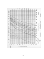
residual gas analyzer (RGA). The RGA is a quadrapole mass spectrometer that can
determine the atomic mass of gas molecules in a system by ionizing the particles
and measuring the change in voltage of an electrode when the ionized gas collides
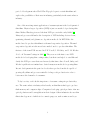
with it. The RGA uses the voltages to then produce cracking patterns used to
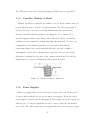
determine the gas composition of the chamber (see figure 1.1).
A substantially low pressure is required to prevent film oxidation and reduce the
contaminant density. A pressure of 10−5 Torr is sufficient, but lower pressures would
help reduce the density of contaminants in the film. At 10−5 Torr the mean free
path of gas in the chamber is approximately 8 meters, which without the unit of
measurement is often referred to as the Knudsen number. The mean free path can
4
Figure 1.1: RGA cracking patterns
be calculated using the following equation
kB T
,
l=√
2πd2 P
(1.1)
where kB is the Boltzman constant, T is the temperature in Kelvin, d is the
diameter of the molecule in meters, and P is the pressure in Pascals. As the mean
free path of the gas particles increases, so does the Knudsen number. When the
Knudsen number is close to or greater than one, gas particles obey principles of free
molecular flow more than viscous flow. The Langmuire-Knudsen equation is
founded on the assumption that the molecules follow a molecular flow regime. The
Langmuire-Knudsen equation is
r
Rm = Cm
M
1
cos θ sin φ 2 (Pe (T ) − P ),
T
r
(1.2)
mol·K
where Rm is the rate per unit area of the source, Cm = 1.85 × 10−2 s·T
a constant,
orr
M is the gram-molecular mass of the deposition material, T is the temperature of
5
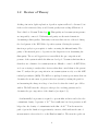
Figure 1.2: Langmuire-Knudsen angle dependence
the deposition material, θ is the angle between the normal of the source and the
substrate, φ is the angle normal to the surface of the substrate and crucible, r is the
distance between the crucible and substrate, and P and Pe are the system pressure
and evaporant partial pressure in Torr respectively. Another assumption of the
Langmuire-Knudsen equation is that the evaporant molecules will travel from the
crucible where they are heated to the substrate without “picking” up any other gas
particles in the chamber (see figure 1.2). Subsequently, a decrease in the base
pressure of the vacuum will also reduce the number of particles “picked” up as they
flow towards the substrate to be deposited.
The Langmuire-Knudsen equation necessitates the use of other methods and
equations to calculate an accurate deposition rate. Among these is Stefan-Boltzman
equation for blackbody radiation:
P = IV = σAT 4 ,
(1.3)
where P is the electrical power through the crucible, I is the current, V is the
voltage, σ is the Stefan-Boltzman constant, is the emissivity, A is the surface area
6
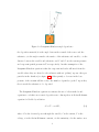
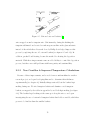
Figure 1.3: Initial deposition system configuration
of the black body, and T is the temperature. Solving for T we find
T =[
IV 1
]4 .
σA
(1.4)
I also used an experimentally derived equation for determining the partial pressure
of liquid Al[5] given by
log P = −
15993
+ 12.409 − 0.999 log T − 3.52 × 10−6 T,
T
(1.5)
where P is the pressure in Torr and T is the temperature. There are, of course,
many other methods capable of deriving the necessary quantities. At the time of the
initial experiment, these were the best approximations available to us, but with the
addition of a type C thermocouple, new vacuum feedthrough, and power supply; our
capability to derive the temperature more accurately has improved. Feasible
alternatives to approximating the crucible temperature solely by using a blackbody
approximation include incorporating power loss/transmission calculations and the
use of a thermocouple.
7
Understanding the fundamentals of vacuum theory can prevent many of the
complications that diminish the accuracy and precision of collected data.
Recognizing the sources of leaks in a vacuum system is one item that is of particular
interest for experimentalists. A variety of sources lead to unwanted gas added to the
chamber by leaks. Vacuum leaks are often due to the pressure gradient that exists
within a vacuum, which creates a surplus of interesting and inimical problems. Thus
vacuum leaks should be addressed prior to experimentation. At a standard
temperature and pressure, almost everything absorbs water vapor and other gases.
One factor that affects how much water vapor is absorbed by a material is the
humidity. Inside a vacuum, these materials release the gases they absorbed because
the same forces that helped trap gasses in them have diminished. As a result,
preparing materials prior to use inside the chamber and considering their impact on
the data is an important step in the experimental process.
All materials will experience some outgassing within a vacuum chamber. A
judicious selection of materials will reduce the effects of outgassing, or leaking of
gas, from materials that are used. For this reason, conditioning of the vacuum
chamber and, if possible, all the materials used in the chamber is also an important
step of experimentation. Chemical cleaning or pre-exposure to vacuum pressures are
both ways to condition materials for use in vacuum. More technical processes such
as those used in developing semiconductors have prescribed standard methods for
cleaning materials prior to use in vacuum.
8
Chapter 2
Experimental Design & Setup
2.1
2.1.1
Vacuum System Design
Recent Developments
BYU-Idaho purchased the vacuum chamber, pressure gauges, roughing pump, and
residual gas analyzer; but received the oil diffusion pump and gate valve as a
donation from another university. The important details about almost all of the
equipment are known. However, we don’t know the material or manufacturer of the
O-ring used with the chamber.
Within the past year, improvements to the vacuum system have helped to achieve
lower pressures more consistently. Initially, the BYU-Idaho vacuum chamber
operated with only a couple thermocouple pressure gauges, ion pressure gauge, oil
diffusion pump backed by a rotary vane roughing pump, viewport, RGA, and single
high voltage electrical feedthrough (The current design can be seen in figure 2.1).
While these are sufficient to achieve pressures suitable for PVD, there is always
room for improvement.
9
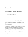
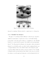
Figure 2.1: BYU-Idaho Vacuum system
The goal that drives development of the vacuum system is that of achieving the
lowest base pressure possible. It is far more difficult to achieve an ultra-high
vacuum than it is to reach a low vacuum. Fortunately, the oil diffusion pump that is
used has a very high throughput rate of about 2,000 L/s. This makes it possible to
achieve pressures as low as 10−8 Torr with the current pump configuration. Despite
this advantage, other elements of the system do more to limit the achievable
pressure than the pump.
2.1.2
Using a Viton Gasket
A pitfall of the current design is lack of smaller ports to transfer materials in and
out of the chamber. The system has a cylindrical design with feedthrough ports
along the sidewall and the chamber separates above the feedthroughs with a 25”
outer diameter (OD) conflat flange (CF) (this can be seen in figure 2.2). The Viton
10
Figure 2.2: 25” OD CF Flange
O-ring that is used, however, makes this flange a possible source of significant
leaking. If a metal gasket and the securing bolts were used this flange wouldn’t be a
big problem.
In order to moderate the side-effects of using a large Viton gasket it must fit
snuggly around the flange. Determining the true size of the O-ring that best fits the
flange is very difficult because small changes in the cut length make the difference
between whether it fits snuggly or not. The equation for calculating the cut length
of an O-ring is
L = π(
OD + ID
),
2
(2.1)
where OD stands for the outer diameter and ID for the inner diameter which is
calculated using:
ID = OD − 2 × (Cs ),
(2.2)
where Cs is the cross sectional diameter of the cord. These equations have been
extremely helpful in determining the appropriate dimensions needed to manufacture
an O-ring.
11
b.
a.
Figure 2.3: O-ring over compression failure
a. reference photo[6] b. actual O-ring
In addition to engineering an O-ring, diagnosing the failure of one is also very
important. In April 2012 the initial O-ring broke due to over-compression, resulting
from too much pressure and high temperatures due to baking. A stable fix to this
obstacle is still in development. After several failed attempts to purchase the
correctly sized O-ring from manufacturers a temporary solution was achieved with a
razor blade and some cyanoacrylate adhesive (super glue). The details of how we
constructed the new O-ring is in appendix D. Minimizing the over-compression and
preventing the breaking of the cyanoacrylate bond of a temporary O-ring is done by
monitoring baking temperatures via an infrared thermometer. Exercising caution in
avoiding the temperature limits, usually 80◦ C, specified by the manufacturer of the
cyanoacrylate will prevent other more serious problems that would ensue if the seal
broke.
2.1.3
Vacuum Conditioning
Vacuum conditioning and upkeep aids in achieving consistent results from in
vacuum experiments. A vacuum system left alone at atmospheric pressure will
require a several days of conditioning prior to use for research, due to water vapor
build-up [7]. We condition our vacuum chamber using two techniques. The first,
12
commonly known as baking, reduces outgassing through heating the chamber walls
and components. The second technique is to backfill the chamber with a dry gas
such as argon, nitrogen, etc., which has a “molecular scrubbing” effect. The
procedure for conditioning the chamber is found in appendix D.
Water vapor is the most detrimental molecule in most vacuum systems. Because
water molecules adsorb easily onto clean surfaces, it is difficult to remove them from
vacuum systems [7]. Removing many of the monolayers of water from the stainless
steel walls takes anywhere from several hours to days. Accelerating desorption of
water molecules is achieved by providing additional energy via heat tape on the
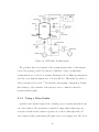
outside of the chamber. An RGA can characterize desorption of water monolayers
during baking (see figure 2.5). Note how the partial pressure due to water vapor
gradually decreases over time. If this same process was repeated without baking,
desorption of water would occur more slowly. Baking via heating tape is a low cost
solution for conditioning a vacuum. There are alternatives that are more effective
such UV radiation and sputtering with an inert gas [7].
In addition to baking, the practice of backfilling, or refilling a vacuum with a dry
gas, is another common technique used to clean systems. Argon is probably the
most common gas used because of its large atomic size, which makes it better for
sputtering off unwanted molecules from chamber walls. However, dry nitrogen is a
more cost effective alternative that also works fairly well. Molecular “scrubbing”
works by adding molecules, in this case nitrogen gas, which then collide with
adsorbed molecules “knocking” them off so they will be pumped out. This is best
done near the crossover pressure of the roughing pump, and requires the use of a
leak vale to precisely control the backfilling of dry nitrogen. The crossover pressure
is the pressure at which the pump can no longer keep up with the gas load it is
under. Carrying out both conditioning processes simultaneously yields better results
13
Figure 2.4: RGA P vs T graph
than they would separately. Implementing additional conditioning methods would
show only minimal improvement until a better process for transfering material into
and out of the chamber is developed so that the 25” flange can remain sealed. The
best practice for keeping a vacuum clean is to avoid putting anything in it that
would contaminate its surfaces.
2.2
2.2.1
Deposition System Design
The Original Experiment
Designing a deposition system is remarkably difficult. Knowing the difficulty, it is
understandable that flashing metal wire created the first films. Essentially, flashing,
or flash evaporation, occurs when you run a high current through a wire so that it
sublimates. The original flashing experiment at BYU-Idaho used a nickel-silver alloy
14
Figure 2.5: Various boats and baskets [1]
wire wrapped around a tungsten wire. Unfortunately, during the flashing the
tungsten sublimated and created a nonhomogeneous film on the glass substrate
instead of the nickel-silver. Research done by Phillip Scott helped improve this
process by exploring the use of boats and baskets (see figures 2.5 and 2.6). In
addition, gradual Joule heating became the method for heating the deposition
material. With these improvements came an added ability to control the deposition
process, but there were still problems with homogeneity and sustainability.
2.2.2
New Crucibles & Improved Temperature Calculations
Because of these improvements, and a need for more uniform films for another
research project, we began developing films and to determine their thickness
experimentally (see chapter 4). Initially things went well, but the baskets kept
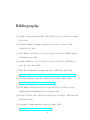
melting during use. We tried tungsten baskets and alumina coated tungsten
baskets, as suggest by the tables in appendix A, and both kept melting (see figure
2.6). The baskets kept breaking at the same spot along the wire so we began
investigating the use of a stranded tungsten basket that holds a crucible, which has
proven to be hardier than the smaller baskets.
15
Figure 2.6: Broken tungsten baskets
An exploration of the theory behind Joule heating revealed the baskets were
breaking because of the wire’s small diameter. Joule proposed that the heat lost by a
wire filament with a known resistance and current passing through it is proportional
to I 2 R, where R represents the resistance. In our case, we assumed all of the power
P was lost in the form of heat through the filament. Thus we approximate that
P = I 2 R.
(2.3)
Incorporating the definition of resistance, which is R ≡ ρ Alcs , where ρ is the
resistivity of the material, l is the length, and Acs is the cross sectional area, we end
up with
P = I 2ρ
l
.
Acs
(2.4)
Using this equation, in conjunction with values found in the CRC Handbook for the
emissivity of tungsten [8] and the Stefan-Boltzman law,
P = σAs T 4 ,
16
(2.5)
Figure 2.7: Broken quartz crucibles
where σ is the Stefan-Boltzman constant, is the emissivity, As is the surface area
of the black body, and T is the temperature; yields
T =[
I 2 lρ 1
]4 .
As Acs σ
(2.6)
This equation can then be used to approximate the temperature of a wire with a
known current running through it. This approximation serves two purposes, first it
explains why the wire baskets began to melt, and second it provides a more
accurate calculation of the temperature for calculating the deposition rate. Hence,
we adopted a crucible and stranded tungsten basket combination. Although the
tungsten wire won’t melt until about 2300◦ C the crucibles will often break well
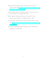
before that temperature (see figure 2.7). For Al deposition, a boron nitride (BN)
crucible works best because of its high thermal conductivity, and thermal resistance
and its low thermal expansion [9]. A BN crucible can sustain temperatures up to
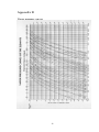
roughly 1800◦ C without breaking. Vapor pressure curves, which can be found in
appendix B, show that the Al will begin to evaporate prior to 1800◦ C in the 10−5 to
10−8 Torr range.
17
2.2.3
Power Supplies & Feedthroughs
Upgrading the heating element meant we also needed to find a more suitable
power supply. The previous power supplies could only provide 20 and 40 amps,
which was not enough to heat the new filament design to an adequate temperature.
Joule heating requires large currents and/or high voltages to accelerate the electrons
traveling through a conductor. Applying a high current is analogous to a large river
of electrons moving through the structure and high voltages are similar to a strong
accelerating force to the electrons. Energy is transferred to the lattice structure of
the conductor as moving electrons ”collide” with other atoms. Increasing the
number of ”collisions” or increasing the energy transferred per collision results in a
greater macroscopic temperature change. To reach our desired temperature, we
purchased a power supply with a power output of 750 watts (60 amps and 12.5
volts). During the research of power supplies, we reassessed the equipment that was
being used and looked for improvements. The high voltage feedthrough we were
using wasn’t suited use with high current. To avoid future complications, we also
purchased a high current feedthrough with solid oxygen free copper (OFE) leads to
help reduce the power loss through the feedthrough pins. Additionally, work was
done to design a new support system for connecting the tungsten filament to the
copper leads. The new configuration can be seen in figure 2.8 and the previous
design in figure 2.9.
2.2.4
Substrate Holder Design
Another feature of the new design is a substrate holder that won’t chip the edges
of the substrates. A substrate is the surface on which films are grown. In theory, the
substrate consists of any type of material. However, the application usually
determines the material that is used (i.e. silicon for semiconductors). As the float
glass substrates were wedged between the threads of two screws positioned above
18
Figure 2.8: New crucible holder configuration
Figure 2.9: Old crucible configuration
19
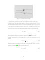
Figure 2.10: Substrate holder design
the deposition source they often chipped and damaged the slides. The remedy to
this problem was to design a new holding system, seen in figure 2.10, and switch the
substrate from float glass slides to round mineral watch glass. A lathe was used to
craft the designed holder from Al; and it was secured in place inside the vacuum
using 4 21 inch steel bolts mounted seated on a 6 inch blank flange on the top of the
chamber.
The design and implementation steps for the vacuum and deposition systems
represent a substantial fraction of my thesis work. However, to fully comprehend
the impact these developments made on the respective systems a deeper explanation
of each individual piece of equipment is given in the next chapter.
20
Chapter 3
Procedures & Documentation
3.1
Equipment Documentation
Purchasing equipment is an important aspect of all experimental physics research.
For further information regarding part numbers or companies from which equipment
was purchased, refer to appendix C. The parts purchased for this project are
detailed in this section.
3.1.1
Silicon Heating Tape
The purpose of the silicon heating tape is strictly for vacuum bakeout. Capable of
heating the chamber to 120◦ C, the heat tape is primarily designed to reduce the
water vapor content of the vacuum chamber. Heating the chamber walls with the
tape gives the sorbed, or adhered, water on the stainless steel the energy needed to
eventually evacuate the system and thereby reducing the overall contribution to the
total pressure from water vapor.
21
Length
72 in
Power density
4.3 W atts/in2
Note: has a high chemical resistance.
Table 3.1: Silicon Heat Tape Specifications
Placing the heat tape flat against the chamber walls during installation provides
the best thermal transfer and can prevent hot spots on the tape during use. In
addition, the tape should not overlap itself at any point. The installer should be
mindful of the proximity of the tape to specific chamber components to prevent
damage to sensitive equipment. When installing the user should make note to only
use high temperature tape to adhere the silicon to the chamber. During use, a
variable transformer in conjunction with the tape will help to control the bakeout
temperature of the chamber. Correct operation of the heat tape leads to lower base
pressures and faster pump down times.
3.1.2
Type C Thermocouple
Thermocouples are capable of providing accurate temperature measurements both
in and out of vacuum. A special feedthrough is required in order to use a
thermocouple within a vacuum. There are several classifications of thermocouples
that cover different temperature ranges and have varying accuracies. A type C
thermocouple is used with the BYU-Idaho vacuum system, as it is capable of
measuring temperatures up to 2300◦ C. By comparing the measured voltage across
two different metals to that of a reference voltage a thermocouple can determine the
temperature. For this process to determine an accurate temperature a cold junction
is often required. We use this thermocouple, in conjunction with power loss
calculations, to help evaluate consistency of our temperature calculations. The
approximation provided by the thermocouple will assist future students in
determining the melting point of the Al. Within the chamber, the hot junction is
22
Temperature Range
0 - 2300 ◦ C
Positive wire
W/5% Re
Negative wire
W/26% Re
Note: Made for use in high and ultra high vacuums.
Table 3.2: Type C thermocouple specifications
placed about an inch from the W filament so a correct temperature is read.
3.1.3
Quartz Crystal Microbalance
The quartz crystal microbalance (QCM) is one of the more costly purchases made
for my research. The purpose of the QCM is to measure the deposition rate of
material onto the substrate. A QCM operates on the piezoelectric principle. During
use, the crystal resonates to a frequency generated by an oscillating circuit. Most
cut crystals are tuned to resonate to a 6 MHz frequency, but as mass is added to the
crystal during the deposition process the frequency of oscillation increases, as
explained by the Saurbrey equation:[10]
2f 2
∆f = − √ 0 ∆m,
A ρ q µq
(3.1)
where ∆f is the change in frequency, δm the change in mass, A the crystal area, f0
g
the resonant frequency, ρq = 2.648 cmg 3 the density of quartz, µq = 2.947 × 1011 cm·s
2
the shear modulus of quartz for the crystal. Positioning the sensor head on the
same spherical wave front as the substrate enables the QCM to provide a reasonable
approximation for the rate of deposition. To correctly position the sensor head, the
water cooling lines that support the sensor were bent, using a tube bending tool, to
an angle slightly past 90◦ C (see figure 3.1). In this position, the QCM software can
be calibrated to provide real time graphs of the rate of deposition and film thickness.
As of the moment, the QCM still needs calibration before it will provide accurate
results. The calibration of the QCM is a project that future students might be
23
Figure 3.1: Quartz Crystal Microbalance Positioning
interested in completing. Calibration should be completed prior to collecting data.
3.1.4
Residual Gas Analyzer
The purpose of a residual gas analyzer (RGA) is to analyze the gas composition
within the vacuum chamber. A quick review of how to use the RGA will help
prolong its life, as all of the repairs for this piece of equipment are costly. The RGA
should not be operated if the base pressure of the chamber reads a pressure higher
than 10−5 Torr. Exposing the hot filament to the atmosphere oxidizes and ruins the
filament. Second, the RGA repeller cage, which looks like a miniature Faraday cage
covering the filament, tends to short with the chamber walls. When the repeller
cage shorts with the chamber the software reads noise around 10−9 Torr. Carefully
bending the repeller cage may fix the problem. If this doesn’t work, you can check
the resistance across the supply and return pins to test if the filament itself is bad.
24
For additional resources and details regarding troubleshooting, see appendix C.
3.1.5
Crucibles, Baskets, & Boats
Thermal deposition is achievable via a number of tools. Boats, baskets, wires, etc.
provide different ways to heat the deposition material. The table in appendix A
describes the best tools to use for heating different materials. As previously
discussed, the first baskets frequently broke during use. So we switched to a
stranded tungsten basked setup. Using a wire basket and crucible combination
facilitates an easy transition to making films with other materials. To avoid cross
contamination, each element should have its own crucible. Knowing the
temperature limits of the crucible material will help to prevent breaking or
damaging the crucible due to thermal stress. Appendix C also provides useful
information regarding the properties of the common materials used for crucibles.
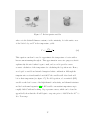
Lastly, figure 3.2 contains an illustration of the current W basket.
Figure 3.2: Crucible & basket combination
3.1.6
Power Supplies
Each power supply that we have used has its own pros and cons. We have used,
or just recently purchased; 20, 40, and 60 amp power supplies. The most capable
power supply is definitely the 60-amp supply both in features and power output. As
with any piece of complex equipment, it would be wise to study the user manual
prior to use. Also, when using any power supply make sure to use the proper gauge
25
Power Output
750 Watts
Max Current
60 Amps
Max Voltage
12.5 Volts
Features: OVP, UVP, Foldback & over-temperature protection
Table 3.3: Genesys 60-12.5 power supply details
for the load cables for the intended power transmission. Connecting several load
cables in parallel works in a pinch to prevent the wires from overheating.
Over voltage protection (OVP) and under voltage protection (UVP) are features of
the Genesys 60-12.5 power supply that allow the user to set a maximum or
minimum output voltage respectively. Foldback protection is an overload protection
feature that lowers the output voltage and current to below normal levels in the
event of a short circuit.
3.2
Vacuum Procedures
As a forewarning, neglecting to follow the outlined procedure for use of the vacuum
chamber may damage pumps, gauges, or the chamber itself. In almost all cases, it is
beneficial to leave the chamber in a low vacuum state. There is no limit to how long
the chamber may remain at low vacuum as the lower pressure helps prevent the
sorbtion of water onto the stainless steel walls. Leaving the oil diffusion pump on at
all times is impractical as the oil takes approximately two hours to cool and may
crack if the power went out.
3.2.1
Pumping to Low Vacuum
1. Turn on the pressure gauge controller and verify that the chamber is
pressurized.
26
2. Close all vent or leak valves that connect the chamber or pumps to the
atmosphere. For the large flange make sure that the Viton O-ring fits snuggly
in its groove before closing the chamber lid.
3. Open the gate valve between the chamber and diffusion pump, and the ball
valve connecting the roughing pump to the diffusion pump.
4. Turn on the roughing pump.
5. Wait until the pressure controller for the chamber reads ∼ 10−3 Torr.
3.2.2
Pumping to High Vacuum
1. Make sure that the thermocouple gauge for the chamber reads ∼ 8 × 10−3 Torr.
2. Turn on the water cooling for the diffusion pump.
3. Plug in the diffusion pump, and wait until the heating element reaches 170◦ C.
4. Wait another five minutes for the diffusion pump to reach approximately 10−5
Torr.
5. Turn on the ion gauge and RGA as necessary.
Procedure for Removing Slides
1. After turning off the power supply and giving the crucible time to cool
proceed with the following steps.
2. If the ion gauge or RGA are on, turn them off.
3. Firmly close the gate valve between the chamber and diffusion pump.
4. Confirm that the valve between the chamber and the roughing pump is also
closed.
5. Vent the chamber.
6. Open the chamber, retrieve/replace the slide, place the Viton O-ring on the
flange, and shut the chamber.
7. Close the vent valve to the chamber.
8. Close the ball valve between the diffusion and roughing pumps. This step
should be done as quick as possible to prevent the diffusion pump from
pressurizing, which can result in cracked oil.
9. Open the valve between the chamber and the roughing pump.
10. Pump down to ∼ 10−3 Torr.
27
11. Open the gate valve and the ball valve.
12. Close the valve between the chamber and roughing pump.
13. Turn on any gauges as necessary.
3.3
Deposition Procedure
The deposition process is still under development. Some factors, such as slide
outgassing, have been investigated but the effects aren’t fully known. It is best to
clean the slides with methanol or isopropyl alcohol and then let cleaning agent
evaporate fully prior to placement in the chamber. Recording more data will help
future students to better tune this process and improve control over film
characteristics.
1. Weigh the glass slide after cleaning and prior to placing it in the chamber.
2. While the chamber is open place a few Al pellets in the BN crucible.
3. Also, position the shield at 55◦ to cover the substrate.
4. After reaching a high vacuum connect the power supply to the feedthrough.
5. Turn on the power supply and turn the voltage control all the way up so the
power output is dependent on the current control knob.
6. Slowly increase the current output. This is done by increasing the output by
3-5 amps and then waiting a few minutes for the crucible to reach a thermal
equilibrium with the W basket.
7. At the desired power output & temperature turn the mechanical feedthrough
clockwise to move the shield out of the way.
8. During deposition record the time elapsed, power supply settings, and the
chamber pressure before and during the deposition process.
9. When done, decrease the current output in the same manner that you
increased it (you can decrement the current in larger amounts) and eventually
turn off the power supply.
10. Lastly, immediately after opening the chamber measure mass of the slide.
28
Chapter 4
Thin Film Deposition Rates
4.1
Initial Rate Calculations
A simple method for approximating the rate of deposition during deposition is done
by weighing the slides pre- and post-deposition and then calculating the average
rate by using equation 4.1. This method is difficult and is prone to many additional
factors that don’t affect rates calculated by equipment such as a QCM. The purchase
of the QCM actually came after this experiment failed to determine a realistic rate.
The rate calculated by the Langmuire-Knudsen equation gives the rate in units of
grams per square centimeter seconds. The experimental rate should look like
Rexp =
m
.
At
(4.1)
The mass m in the equation is the change in mass, or the mass of Al deposited, of
the slide. Measuring the slide pre and post deposition is an easy task, but the scale
used needs to be capable of measuring differences of milligrams at minimum.
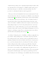
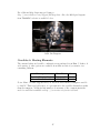
Calculating the filmed area of the slide required a more creative approach. After
projecting a filmed slide onto a wall and tracing the filmed area onto grid paper, we
were able to approximate the deposition area via a scale and the number of filmed
squares on the grid paper. Figure 4.1 shows a copy of the grid paper where the
29
Figure 4.1: Filmed slide projection
shaded squares represent the filmed area.
Assuming no angular dependence in the Langmuire-Knudsen equation further
simplifies the theoretical model to look like
r
Rm = Cm
M 1
(Pe (T ) − P ).
T r2
(4.2)
This justification is acceptable given the crucible is positioned directly beneath and
sufficiently far from the substrate[11]. An appropriate distance should meet the
requirement that the mean free path of molecules in the chamber be much greater
than the distance between the crucible and substrate. Black body temperature
approximations include an emissivity factor relating to the fraction of power that is
emitted as radiation. For initial calculations we used an emissivity of one.
Realistically the emissivity of tungsten between 1700 and 2500◦ C is roughly 0.41 [8].
Using an accurate emissivity doesn’t change the outcome of the early experiment.
30
The uncertainty in the temperature calculations was the biggest factor affecting the
deposition rate calculations. Initial temperature calculations had an uncertainty of
±75◦ C. Improving the accuracy of temperature calculations may make this method
reasonable.
Calculating the uncertainties associated with the composition of equations is a
mathematical mess. MATLAB code for analyzing the data and determining the χ2ν
value is in appendix F. This code accounts for the effects of slide outgassing while in
vacuum by adding an empirically calculated amount as well as a coefficient for the
black body emissivity and its related uncertainty.
The data from the experiment indicates that our model is far from accurate. Data
from eleven slides was analyzed to compare the theoretical deposition rate under the
given conditions and deposition time to the experimentally calculated rate. The
reduced χ2 value was around 3.3 × 107 . This alludes to the inadequacy of the tested
model in calculating the deposition rate of Al vapor. Despite the results the
experiment was useful in determining several areas of improvement for the
deposition system and the process used for calculating rates.
4.2
Effects of Slide Outgassing
After measuring a post-deposition slide mass that was less than its pre-deposition
weight, we realized that the mineral glass must have been outgassing. So we devised
an experiment to quantify the slide outgassing. Determining how much a material
outgasses is simple. After cleaning each slide individually and letting the methanol
evaporate off, they were weighed and placed inside the vacuum chamber. To
maintain a controlled environment all of the slides were placed side-by-side inside
31
the vacuum for the same length of time. After several hours the slides were removed
and weighed. Weighing each slide daily for several days after the experiment
provided additional insight about the environmental effects on the slide’s weight.
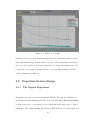
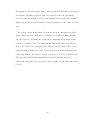
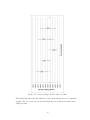
Figures 4.2 and 4.3 show the change in each slides weight over the course of several
days.
The average change in slide mass between pre and post outgassing was 0.0012
grams. This is the same value used to adjust for the weight lost during the film
deposition process. Adjusting the weight due to outgassing effects improves the
accuracy of calculated rates. Producing thicker films in the future would negate
most of the effects from outgassing as the difference in slide mass would be more
significant with a thicker layer of Al deposited on them. Further inquiry into the
causes that influence the weight of a slide on a given day would be helpful as well.
The data suggests that environmental factors such as humidity and room
temperature may play a more crucial role in the weight of a slide than was at first
believed.
32
Figure 4.2: Average change in slide mass over time
The initial time interval is the difference between the initial and post outgassing
weights. The error bars also provide the high and low deviation from the mean
change in mass.
33
Figure 4.3: Change in slide mass between consecutive days
34
Chapter 5
Future Experiments & Summary
Fully automating the deposition system is still a long ways down the road. This
means there is an ample supply of projects left for future students. Developing the
system will expand the research opportunities for future students enabling them to
conduct experiments requiring the use of films. Since we are now able to
consistently produce films, students may want to work on improving film quality
and deposition rate calculations. In addition, it may interest some students to look
into alternative deposition methods.
5.1
Improving Film Quality
There are two sides to improving film quality. The first is the ability to recognize
and characterize a films quality. This is known as film tribology. The other side
emphasizes applying methods for ensuring the desired film characteristics during
deposition. Film tribology requires additional equipment that we currently don’t
own. Using this equipment characteristics of films such as adhesion, hardness, and
homogeneity can be determined. Some of the tribology methods are also an effective
35
at determining film thickness after deposition. Students wanting to learn more
about film tribology would find the Handbook of Hard Coatings helpful in their
research[12]. This book also contains ample information regarding many CVD and
PVD methods and their theory.
An important step in building a quality deposition system is implementing
preventative methods. Better substrate preparation is one item requiring more
attention, and something that would definitely improve the film quality. Typical
substrate preparation often involves chemical etching and cleaning prior to
deposition followed by heating during and after deposition to anneal the film and/or
bias the substrate surface. These methods would also require new equipment.
Methods such as e-beam or sputter deposition can also provide improved film
quality and purity. Ample resources regarding the best practices regarding film
quality are available in many of the cited texts.
5.2
Improved Deposition Rates
During the rates experiment we made several questionable approximations to
calculate our theoretical rates. A few alternative approximations still exist that may
improve results. This may lead to practical application in calibrating the QCM and
use with films of other materials. Analyzing the magnitude of uncertainties of
variables in an experiment can be quite revealing of what needs improvement. Such
is the case with the deposition rates, and the variable with the largest uncertainty is
the temperature. We believe the large uncertainty in the temperature to be related
to the significant amount of power that is lost by the load cables. Preliminary
calculations suggest that the actual voltage across the W basket used to heat the
crucible is significantly less than previously believed. Incorporating the loss of
36
power during transmission may improve the accuracy and precision of the calculated
temperature.
These projects are just a few of many that would be valuable for future students
wanting to work with the BYU-Idaho vacuum and deposition systems. Excellent
opportunities for research still exist for students. Unlike the deposition system, the
vacuum system has limited room for further development without conducting a
complete overhaul. However, this doesn’t limit the possibilities for research in any
way.
37
Bibliography
[1] John L. Vossen and Werner Kern. Thin Film Processes II. Boston: Academic
Press, 1991.
[2] James M. Lafferty. Vacuum: from art to exact science. Physics Today,
34(11):211–231, 1981.
[3] D.M. Mattox. Foundations of Vacuum Coating Technology. William Andrew
Publishing/Noyes, 2003.
[4] John F. O’Hanlon. A User’s Guide to Vacuum Technology. John Wiley ’&’
Sons, Inc., 3rd edition, 2003.
[5] Wake Forest University. Vacuum evaporation. PDF, Mar. 2012. URL:
http://users.wfu.edu/ucerkb/Nan242/L06-Vacuum_Evaporation.pdf.
[6] Problem Solving Problems Inc. O-ring and seal failure [online]. URL:
http://www.pspglobal.com/abrasion.html.
[7] D.M. Mattox. Handbook of Physical Vapor Deposition (PVD) Processing.
William Andrew Publishing/Noyes, 1st edition, 1998.
[8] Robert C. Weast, editor. Handbook of Chemistry and Physics. CRC Press, Inc.,
66th edition, 1985.
[9] Accuratus. Ceramic materials’ character [online]. URL:
http://accuratus.com/materials.html.
38
[10] Stanford Research Systems. Quartz crystal microbalance theory and
calibration. PDF. URL: http://www.thinksrs.com/downloads/PDFs/
ApplicationNotes/QCMTheoryapp.pdf.
[11] M. A. Herman, H. Sitter, and W. Richter. Epitaxy: Physical Principles and
Technical Implementation. Springer-Verlag, 2010.
[12] R. F. Bunshah. Handbook of Hard Coatings. Norwich, N.Y.: Noyes
Publications and Park Ridge, N.J.: William Andrew Pub., 2001.
[13] Jonathan Stolk. Materials guide for thermal evaporation [online]. Jan. 2012.
URL: http://www.lesker.com/newweb/menu_depositionmaterials.cfm?
section=MDtable.
[14] Dr. Walter Umrath. Fundamentals of vacuum technology. Technical report,
Oerlikon Leybold Vacuum, 2007.
39
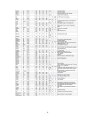
Appendix A
Materials Guide for Thermal Evaporation
Adapted from Kurt J.Lesker Co. [13]
40
41
Appendix B
Vapor pressure curves
42
43
44
Appendix C
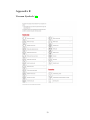
Equipment Purchasing Information
Type C Thermocouple
Purchased from Kurt J. Lesker, which can be found online at www.lesker.com.
Description
Part No.
Cost
Type C CF Feedthrough TFT3CY00003 $295.00
Alloy 405/426 Wire*
FTAWC056
$10.00
Note(s): *This is the type C thermocouple wire.
Quartz Crystal Microbalance (QCM)
Purchased from Sycon Instruments, which can be found online at www.sycon.com.
The QCM was purchased as a package with the STM2 and the out of vacuum BNC
cable. The in vacuum microdot cable was purchased separately. All parts can be
purchased directly from the company.
Description
Part No.
6 Mhz Gold Coated Sensor Crystals 10pk
500-117
Vacuum Feedthrough
500-017
Single Head Sensor
500-042
Oscillator & Transducer (STM-2)
500-408
30” Microdot Cable
500-024
10” Vacuum Microdot Cable
500-023
Cost
$67.00
$491.00
$375.00
$620.00
$80.00
N/A
Notes: The microdot cable shouldn’t be further than 30” from the sensor head while
using the STM-2. Despite this we’ve tried to see if the STM-2 will still work with
our 30” microdot cable. Preliminary findings have yielded no significant results
because the power supply couldn’t heat the material to a temperature that a
substantial deposition rate could be detected. Additionally, the water cooling for
the sensor head should be used in the future to reduce noise and improve accuracy.
Power Supplies
Several power supplies were used for thin film deposition at BYU-Idaho, but the
only one purchased during my research was from TDK. The website url that the
technical details can be found at is
http : //www.us.tdk − lambda.com/hp/producth tml/genh.htm.
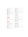
45
Description
Part No.
Cost
12.5V 60A Power Supply GENH 12.5-60 $1890.00
Note(s): We purchased the additional USB option
Viton O-ring
Viton is used because of its low permeation rate at low pressures, and because it is
resistant to many chemicals. Viton-A is the standard material used for vacuum
system seals. A quick google search should provide several companies that are
willing to sell Viton-A cord stock, which you can use to make your own O-rings. We
are still working with a company called Quick Cut Gasket to make us some custom
O-rings, but this process is time consuming and we haven’t found a good fit yet.
When purchasing Viton cord stock make sure you buy stock that has a cross section
(CS) 0.108 inches.
Heating Tape
Purchased from BriskHeat at www.briskheat.com.
Description
1” x 96” Silicone Heat Tape
High Temperature Tape
Part No.
Cost
BS0101080L $173.65
PSAT36A
$16.00
Notes: The high temperature adhesive tape is made to function up to 80◦ C, but
we’ve used it past this temperature and it has held the tape in place at around
125◦ C.
Mineral Glass Slides
Several companies sell mineral glass slides, but they don’t often refer to them as
slides. You will find better results for a Google search using the term ”watch glass”.
Due to the effects of outgassing of the mineral glass it is best that you try and
purchase the thinnest slides possible. The substrate holder is designed to hold slides
that are 1” or (25.4mm) in diameter.
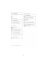
Residual Gas Analyzer (RGA)
Replacement equipment & more detailed documentation can be found at
www.thinksrs.com.
Description
Part No.
200 amu RGA
RGA200
ThO2Ir Replacement Filament
O100RF
Replacement Ionizer Kit
O100RI
46
Cost
$4750.00
$200.00
$450.00
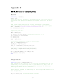
For additional help diagnosing problems see
http : //www.thinksrs.com/support/RGAsup.htm. Also, the RGA pin diagram
from ThinkSRS’ website is available below.
RGA Pin Diagram
Crucibles & Heating Elements
The current basket and crucible combination was purchased from Kurt J. Lesker. A
wide variety of other options are available from their website if you want to try
something different.
Description
Part No.
Cost
Stranded Tungsten Basket EVB8A3025W $34.00
Boron Nitride Crucible
EVC1BN
$34.00
Notes: Kurt J. Lesker suggests that you only heat their stranded tungsten crucible
to 1800◦ C. This is probably more of a precaution for the crucibles themselves rather
than the tungsten. Additional information about many of the common materials
used for crucibles is available at http : //accuratus.com/materials.html.
47
Gas Leak Valve
This item was made by Varian, but was purchased from Ebay. Equivalent leak
valves are sold by Kurt J. Lesker and other companies, but the cost is significantly
greater than those sold on Ebay.
Description
Varian Leak Valve
Part No.
N/A
48
Cost
$80.00
Appendix D
Equipment Troubleshooting & Repair
O-ring Construction Procedure
This step-by-step process describes the procedure used to construct a temporary
O-ring for use with the 25” OD CF Flange of the vacuum chamber. Only Viton-A
cord with a cross section of 0.108 in. should be used in the construction of this
O-ring.
• First, as with any process involving a vacuum system, you should put on
powder-free gloves.
• Take the old O-ring and cut it once so that it forms one long cord.
• Tape the old O-ring to a flat surface in a straight line. You may find the
straight edge of a meter stick to be helpful in placing the cord in a straight
line.
• Place the new cord stock next to the old O-ring with one end of the cord
stock flush to one end of the old O-ring and tape it down if needed.
• Next, using the razor blade and a squaring tool, cut the cord stock
perpendicular to the cord so that it is the same length as the old O-ring.
• Then perpendicularly cut a small amount of cord stock (about 1mm) off the
other end of the newly cut Viton cord.
• At this point, in order to ensure a better bond between the cyanoacrylate
and the Viton, both ends should be cleaned with isopropyl alcohol and allowed
15-20 minutes to dry.
• Once the alcohol has evaporated off of the Viton you will then place a small
drop of cyanoacrylate on one end of the newly cut cord stock and the hold the
ends together gently until the cyanoacrylate holds.
• Gently place the new O-ring in a safe location and let it cure for an hour or
two before using.
This method will produce a stable O-ring capable of functioning properly under
mild baking (less than 80◦ C) that should last long enough to order a new O-ring.
49
Appendix E
Vacuum Symbols [14]
50
51
52
Appendix F
MATLAB Code for Analyzing Data
Rates.m
function [] = Rates()
clear; clc;
%Using the Vapor.m, Knudsen.m, and Temperature.m files this function
%calculates the appropriate reduced Chi-squared values for the data
%set.
%The column order should be as follows, pre-weight, post-weight,
%pressure, pressure uncertainty, current, voltage, and time elapsed
Data = xlsread('E:/Film Calculations/RateData.xlsx');
N = size(Data(1,:),2);
%Separating the data
Pre = Data(:,1);
Post = Data(:,2);
P = Data(:,3).*133.322368; %converting from Torr to Pa
P_u = Data(:,4).*133.322368;
C = Data(:,5);
V = Data(:,6);
Time = Data(:,7);
%Calculating theoretical values & uncertainties
[T,T_u] = Temperature(C,V);
[Pp,Pp_u] = Vapor(T,T_u);
[R,R_u] = Knudsen(T,T_u,Pp,Pp_u,P,P_u);
%Calculating actual values & uncertainties
[Rex,Rex_u] = Experimental(Pre,Post,Time);
Chi = sum(sum((R-Rex).^2)./(Rex_u.^2))
Chi_reduced = Chi/(N-1)
end
Temperature.m
function [T,T_u] = Temperature(C,V)
%The purpose of this function is to calculate the Temperature and its
%uncertainty for a black body with a given emissivity (eps). This is
%done using a combination of Joule's power relation for resistive
%heating and Ohm's law for resistors.
%This function assumes an uncertainty in the voltage and current of 0.1
%A/V respectively
sig = 5.67*10^(-8); %Stefan-Boltzmann constant
53
eps = 0.41; %emissivity of W between ~1700-2500 degree C
eps_u = 0.05; %the rough uncertainty of the emissivity
A = 0.00005141; %crucible surface area
A_u = 0.00000025; %uncertainty in the surface area
C_u = 0.1; %uncertainty in current
V_u = 0.1; %uncertainty in voltage
%There is a constant term in the partial derivative of T
dT_cons = (1/4)*(C.*V./(sig*eps*A)).^(-3/4);
%Calculating T
T = (C.*V./(sig*eps*A)).^(1/4);
%Calculating the uncertainty in T
T_u = sqrt( (C_u^2)*(dT_cons.*(V/(sig*eps*A))).^2 +... %current term
(V_u^2)*(dT_cons.*(C/(sig*eps*A))).^2 +... %voltage term
(eps_u^2)*(dT_cons.*(-C.*V/(sig*eps^2*A))).^2 +...
%emissivity
(A_u^2)*(dT_cons.*(-C.*V/(sig*eps*A^2))).^2); %area term
end
Vapor.m
function [Pp, Pp_u] = Vapor(T, T_u)
%This function is designed to calculate the experimental vapor pressure
%and its associated uncertainties due to heated Al at a given
%temperature as given by Wake Forest University's lab report.
%Calculate the partial pressure
Pp = 10.^((-15993./T) + 12.409 - 0.999*log10(T) - 3.52*10^(-6)*T);
%Calculate the uncertainty in the partial pressure
%If y = 10^x, then
%dy/dx = (10^x)*(ln 10)
Pp_u = sqrt((T_u.^2).*((Pp*log(10)).^2));
end
Knudsen.m
function [R,R_u] = Knudsen(T,T_u,Pp,Pp_u,P,P_u)
%This function calculates the deposition rate and its uncertainty using
%the angular independent form of the Langmuire-Knudsen relation.
Cm = 1.85*10^(-2); %a constant term
M = 26.9815386; %gram molecular mass of Al (courtesy of Wolfram Alpha)
54
r = 16.3; %source-substrate distance in cm
r_u = 0.5; %uncertainty in r
%Calculate R
R = Cm*sqrt(M./T).*(1/(r.^2)).*(Pp - P);
%Calculate the uncertainty in R
R_u = sqrt( (r_u^2)*(R.*(-2./r)).^2 +... %distance term
(T_u.^2).*((1-2)*(M./(T.^2)).*(M./T).^(-1)).^2 +... %T term
(P_u.^2).*(-Cm*sqrt(M./T).*(1/(r^2))).^2+... %P term
(Pp_u.^2).*(Cm*sqrt(M./T).*(1/(r^2))).^2); %Pp term
end
Experimental.m
function [Rex,Rex_u] = Experimental(Pre,Post,Time)
%This function calculates the experimental deposition rates. This is
%done assuming the uncertainty in the deposition time to be constant,
%and accounting for slide outgassing by a constant adjustment factor in
%weight.
A = 2.68; %film surface area measure through scale projection method
(cm^2)
A_u = 0.08; %uncertainty in film surface area
out = 0.0012; %outgassing mass adjustment
Time_u = 1.5; %a generous uncertainty of 1.5 seconds
M_u = 0.0007; %uncertainty in the difference of mass measurement
%Calculating the difference in mass pre & post deposition
M = (Post + out) - Pre;
%Experimental rate calculation
Rex = M./(A.*Time);
%Experimental rate uncertainties
Rex_u = sqrt( (M_u^2)*(1./(A*Time)).^2 +... %mass term
(Time_u^2)*(-1*(M./(A*Time.^2))).^2 +... %time term
(A_u^2)*(-1*(M./(A^2*Time))).^2); %area term
end
55
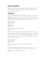
Power Loss Calculator
This file should provide an approximate power lost during Joule heating on standard
annealed copper wire. The purpose of which is to better estimate the power input
provided by our power supply in order to better calculate the deposition rate of the
material in our vacuum chamber.
Assumptions
For this calculation I'm assuming that the temperature of the wire doesn't change. The
length of the wire is also assumed to be fixed (aka no thermal expansion). I'm also
assuming that the gauge of the copper fixture inside the vacuum chamber is negligible.
As of the moment, I'm also assuming that the resistivity of my wires per 1000 ft (values
obtained from CRC F-114) is constant for both my 10 & 18 AWG wire.
R10 = 0.9989/304.8;
R18 = 6.385/304.8;
Length1 = 1;
Length2 = 0.7;
Current = 23.0;
Pow = 46.0;
Current^2*(R10*Length1 + R18*Length2)
%/Pow
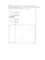
This means that I'm losing almost 10 watts of power initially through my wires when I
start it up. That is about 20% of my power lost through heat to the room. Lets see how
much I lose when I add two more 18 AWG wires in parallel with my first 18 AWG wire.
In this case though, I should note that my resistivty/meter coefficients are different (for
this case I'll assume that the 18 gauge wire is hot ~75 degrees Celsius & the 10 gauge
wire is still ~50 degrees Celsius).
R10 = 1.117/304.8;
R18 = 7.765/304.8;
Current = 39.0;
Pow = 237.9;
Current^2*(R10*Length1) + (1/3*Current)^2*(3*R18*Length2)
%/Pow
This means I'm losing roughly 14 watts at full power, which is roughly 6% of my total
power input. Not a surprising amount, but I could use those extra 14 watts.
R[wlength_,rconst_] = rconst/304.8*wlength;
cmax = 42;
56
57