Download Lab 2: Getting familiar with LabVIEW: Part II

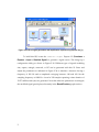
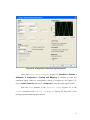
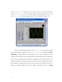
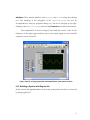
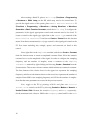
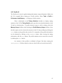
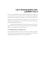
Lab 2: Getting familiar with
LabVIEW: Part II
Now that an initial familiarity with the LabVIEW programming environment has
been acquired in Lab 1, this second lab covers an example where a simple DSP
system is built, thus enhancing the familiarity of the reader with LabVIEW. This
example involves a signal generation and amplification system. The shape of the
input signal (sine, square, triangle, or saw tooth) as well as its frequency and gain are
altered by using appropriate FP controls.
The system is built with Express VIs first, then the same system is built with
regular VIs. This is done in order to illustrate the advantages and disadvantages of
Express VIs versus regular VIs for building a system.
L2.1 Building a System VI with Express VIs
The use of Express VIs allows less wiring on a BD. Also, it provides an interactive
user-interface by which parameter values can be adjusted on the fly. The BD of the
signal generation system using Express VIs is shown in Figure 2-33.
1
Figure 2-33: BD of signal generation and amplification system using Express VIs [1].
To build this BD, locate the Simulate Signal Express VI (Functions »
Express » Input » Simulate Signal) to generate a signal source. This brings up a
configuration dialog as shown in Figure 2-34. Different types of signals including
sine, square, triangle, sawtooth, or DC can be generated with this VI. Enter and
adjust the parameters as indicated in Figure 2-34 to simulate a sinewave having a
frequency of 200 Hz and an amplitude swinging between -100 and 100. Set the
sampling frequency to 8000 Hz. A total of 128 samples spanning a time duration of
15.875 milliseconds (ms) are generated. Note that when the parameters are changed,
the modified signal gets displayed instantly in the Result Preview graph window.
2
Figure 2-34: Configuration of Simulate Signal Express VI.
Next, place a Scaling and Mapping Express VI (Functions » Express »
Arithmetic & Comparison » Scaling and Mapping) to amplify or scale this
simulated signal. When its configuration dialog is brought up, see Figure 2-35,
choose Linear (Y=mx+b) and enter 5 in Slope (m) to scale the input signal 5 times.
Wire the Sine terminal of the Simulate Signal Express VI to the
Signals terminal of the Scaling and Mapping Express VI. Note that a wire
having a dynamic data type gets created.
3
Figure 2-35: Configuration of Scaling and Mapping Express VI.
To display the output signal, place a Waveform Graph (Controls » Modern
» Graph » Waveform Graph) on the FP. The Waveform Graph can also be created
by right-clicking on the Scaled Signals terminal and choosing Create » Graph
Indicator from the shortcut menu.
Now, in order to observe the original and the scaled signal together in the
same graph, wire the Sine terminal of the Simulate Signal Express VI to the
Waveform
Graph. This inserts a Merge
Signals function on the wire
automatically. An automatic insertion of the Merge Signals function occurs when
a signal having a dynamic data type is wired to other signals having the same or
other data types. The Merge Signals function combines multiple inputs, thus
allowing two signals, consisting of the original and scaled signals, to be handled by
4
one wire. Since both the original and scaled signals are displayed in the same graph,
resize the plot legend to display the two labels and markers. The use of the dynamic
data type sets the signal labels automatically.
To run the VI continuously, place a While Loop. Position the While Loop
to enclose all the Express VIs and the graph. Now the VI is ready to be run.
Figure 2-36: FP of signal generation and amplification system.
Run the VI and observe the Waveform Graph. The output should appear as
shown in Figure 2-36. To extend the plot to the right-end of the plotting area, rightclick on the Waveform Graph and choose X Scale, then uncheck Loose Fit from
the shortcut menu. The graph shown in Figure 2-37 should appear.
5
Figure 2-37: Plot with Loose Fit.
If the plot runs too fast, a delay can be placed in the While Loop. To do this,
place a Time Delay Express VI (Functions » Programming » Timing » Time
Delay) and set the delay time to 0.2 in the configuration window. This way, the loop
execution is delayed by 0.2 seconds in the BD shown in Figure 2-33.
Although this system runs successfully, no control of the signal frequency
and gain is available during its execution since all the parameters are set in the
configuration dialogs of the Express VIs. To gain such a flexibility, some
modifications need to be made.
To change the frequency at run time, place a Vertical Pointer Slide
control (Controls » Modern » Numeric » Vertical Pointer Slide) on the FP and
wire it to the Frequency terminal of the Simulate Signal Express VI. The
control is labeled as Frequency. The Express VI can be resized to show more
6
terminals at the bottom of the expandable node. Resize the VI to show an additional
terminal below the Sine terminal. Then, click on this new terminal, error out by
default, to select Frequency from the list of the displayed terminals.
Next, replace the Scaling and Mapping Express VI with a Multiply
function (Functions » Programming » Numeric » Multiply). Place another
Vertical Pointer Slide control and wire it to the y terminal of the Multiply
function to adjust the gain. This control is labeled as Gain. These modifications are
illustrated in Figure 2-38.
Figure 2-38: BD of signal generation and amplification system with controls.
Now on the FP, set the maximum range of each slide control to 1000 for the
Frequency control and 5 for the Gain control, respectively. Also, set the default
values for these controls to 200 and 2, respectively.
By running this modified VI, it can be observed that the two signals get
displayed with the same label since the source of these signals, i.e. the Sine terminal
7
of the Simulate Signal Express VI, is the same. Also, due to the autoscale feature
of the Waveform Graph, the scaled signal appears unchanged while the Y axis of
the Waveform Graph changes appropriately. This is illustrated in Figure 2-39.
Figure 2-39: Autoscaled graph of two signals shown together.
Let us now modify the property of the Waveform Graph. In order to disable
the autoscale feature, right-click on the Waveform Graph and uncheck Y Axis »
AutoScale Y. The maximum and minimum scale can also be adjusted. In this
example -600 and 600 are used as the minimum and maximum values, respectively.
This is done by modifying the maximum and minimum scale values of the Y axis
with the Labeling tool. If the automatic tool selection mode is enabled, just click on
the maximum or minimum scale of the Y axis to enter any desired scale value. To
modify the labels displayed in the plot legend, right-click and choose Ignore
8
Attributes. Then, edit the labels to read Original and Scaled using the Labeling
tool. The changing of the properties of the Waveform Graph can also be
accomplished by using its properties dialog box. This box is brought up by rightclicking on the Waveform Graph and choosing Properties from the shortcut menu.
The completed FP is shown in Figure 2-40. With this version of the VI, the
frequency of the input signal and the gain of the output signal can be controlled
using the controls on the FP.
Figure 2-40: FP of signal generation and amplification system with controls.
L2.2 Building a System with Regular VIs
In this section, the implementation of the same system discussed above is achieved
by using regular VIs.
9
After creating a blank VI, place a While Loop (Functions » Programming
» Structures » While Loop) on the BD, which may need to be resized later. To
provide the signal source of the system, place a Basic Function Generator VI
(Functions » Programming » Waveform » Analog Waveform » Waveform
Generation » Basic Function Generator) inside the While Loop. To configure the
parameters of the signal, appropriate controls and constants need to be wired. To
create a control for the signal type, right-click on the signal type terminal of the
Basic Function Generator VI and choose Create » Control from the shortcut
menu. Note that an enumerated (Enum) type control for the signal gets located on the
FP. Four items including sine, triangle, square, and sawtooth are listed in this
control.
Next, right-click on the amplitude terminal, and choose Create » Constant
from the shortcut menu to create an amplitude constant. Enter 100 in the numeric
constant box to set the amplitude of the signal. In order to configure the sampling
frequency and the number of samples, create a constant on the sampling
information terminal by right-clicking and choosing Create » Constant from the
shortcut menu. This creates a cluster constant which includes two numeric constants.
The first element of the cluster shown in the upper box represents the sampling
frequency and the second element shown in the lower box represents the number of
samples. Enter 8000 for the sampling frequency and 128 for the number of samples.
Note that the same parameters were used in the previous section.
Now, toggle to the FP by pressing <Ctrl-E> and place two Vertical
Pointer Slide controls on the FP by choosing Controls » Modern » Numeric »
Vertical Pointer Slide. Rename the controls Frequency and Gain, respectively.
Set the maximum scale values to 1000 for the Frequency control and 5 for the Gain
10
control. The Vertical Pointer Slide controls create corresponding icons on
the BD. Make sure that the icons are located inside the While Loop. If not, select
the icons and drag them inside the While Loop. The Frequency control should be
wired to the frequency terminal of the Basic Function Generator VI in order
to be able to adjust the frequency at run time. The Gain control is used at a later
stage.
The output of the Basic Function Generator VI appears in the
waveform data type. The waveform data type is a special cluster which bundles
three components (t0, dt, and Y) together. The component t0 represents the trigger
time of the waveform, dt the time interval between two samples, and Y data values
of the waveform.
Next, the generated signal needs to be scaled based on a gain factor. This is
done by using a Multiply function (Functions » Programming » Numeric »
Multiply) and a second Vertical Pointer Slide control, named Gain. Wire the
generated waveform out of the signal out terminal of the Basic Function
Generator VI to the x terminal of the Multiply function. Also, wire the Gain
control to the y terminal of the Multiply function.
Recall that the Merge Signals function is used to combine two signals
having dynamic data types into the same wire. To achieve the same outcome with
regular VIs, place a Build Array function (Functions » Programming » Array »
Build Array) to build a 2D array, i.e. two rows (or columns) of one dimensional
signal. Resize the Build Array function to have two input terminals. Wire the
original signal to the upper terminal of the Build Array function, and the output
of the Multiply function to the lower terminal. Remember that the Build Array
function is used to concatenate arrays or build n-dimensional arrays. Since the
11
Build Array function is used for comparing the two signals, make sure that the
Concatenate Inputs option is unchecked from the shortcut menu. More details on
the use of the Build Array function can be found in [2].
A Waveform Graph (Controls » Modern » Graph » Waveform Graph) is
then placed on the FP. Wire the output of the Build Array function to the input of
the Waveform Graph. Resize the plot legend to display the labels and edit them.
Similar to the example in the previous section, the AutoScale feature of the Y axis
should be disabled and the Loose Fit option should be unchecked along the X axis.
Place a Wait (ms) function (Functions » Programming » Timing » Wait)
inside the While Loop to delay the execution in case the VI runs too fast. Rightclick on the milliseconds to wait terminal and choose Create » Constant
from the shortcut menu to create and wire a Numeric Constant. Enter 200 in the
box created.
Figure 2-41 and Figure 2-42 illustrate the BD and FP of the designed signal
generation system, respectively. Save the VI as Lab02_ Regular_Waveform.vi and run
it. Change the signal type, gain and frequency values to see the original and scaled
signal in the Waveform Graph.
12
Figure 2-41: BD of signal generation and amplification system using regular VIs.
Figure 2-42: Original and scaled output signals.
13
The waveform data type is not accepted by all the functions or subVIs. To
cope with this issue, the Y component (data value) of the waveform data type is
extracted to have the output signal as an array of data samples. This is done by
placing a Get Waveform Components function (Functions » Programming »
Waveform » Get Waveform Components). Then, wire the signal out terminal
of the Basic Function Generator VI to the waveform terminal of the Get
Waveform Components function. Click on t0, the default terminal, of the Get
Waveform Components function and choose Y as the output to extract data values
from the waveform data type, see Figure 2-43. The remaining steps are the same as
those done for the version shown in Figure 2-41. In this version, however, the
processed signal is an array of double precision samples.
Figure 2-43: Matching data types.
14
L2.3 Profile VI
The Profile tool is used to gather timing and memory usage information. Make sure
the VI is stopped before setting up a Profile window. Select Tools » Profile »
Performance and Memory … to bring up a Profile window.
Place a checkmark in the Timing Statistics checkbox to display timing
statistics of the VI. The Timing Details option provides more detailed statistics of the
VI such as drawing time. To profile memory usage as well as timing, check the
Memory Usage checkbox after checking the Profile Memory Usage checkbox. Note
that this option can slow down the execution of the VI. Start profiling by clicking the
Start button on the profiler, then run the VI. A snapshot of the profiler information
can be obtained by clicking on the Snapshot button. After viewing the timing
information, click the Stop button. The profile statistics can be stored into a text file
by clicking the Save button.
An outcome of the profiler is exhibited in Figure 2-44 after running the
Lab02_Regular VI. More details on the use of the Profile tool can be found in [3].
15
Figure 2-44: Profile window after running Lab02_Regular VI.
L2.4 Bibliography
[1]
National Instruments, Getting Started with LabVIEW, Part Number 323427A01, 2003.
[2]
National Instruments, LabVIEW User Manual, Part Number 320999E-01, 2003.
[3]
National Instruments, LabVIEW Performance and Memory Management,
Application Note 168, Part Number 342078B-01, 2004.
L2.5 Lab Experiments
Carry out the following experiments with and without the MathScript feature of
LabVIEW 8.
1. Build a VI to generate two sinusoid signals with the frequencies f1 Hz and f2 Hz
and the amplitudes A1 and A2, based on a sampling frequency of 8000 Hz with
16
the number of samples being 256. Set the frequency ranges from 100 Hz to 400
Hz and set the amplitude ranges from 20 to 200. Generate a third signal with the
frequency f3 = (mod (lcm (f1, f2), 400) + 100) Hz, where mod and lcm denote the
modulus and least common multiple operation, respectively, and the amplitude
A3 being the sum of the amplitudes A1 and A2. Use the same sampling frequency
and number of samples as used for the first two signals. Display all the signals
using the legend on the same waveform graph and label them accordingly. When
not using the MathScript feature, it is easier to use the Express VIs.
2. Build a VI to check whether a given positive integer ‘n’ is a prime number or not
and display a warning message if it is not a prime number.
3. Build a VI to generate two sinusoid signals the same as the ones in Experiment 2.
Generate a third signal with the frequency f3 = (gcd (f1, f2) + mean (f1, f2)) Hz,
where gcd and mean denote the greatest common divisor and the average
operation, respectively, and the amplitude A3 being the sum of the amplitudes A1
and A2. Use the same sampling frequency and number of samples as used for the
first two signals. Display all the signals using the legend on the same waveform
graph and label them accordingly. When not using the MathScript feature, it is
easier to use the Express VIs.
4. Build a VI to generate the first ‘n’ prime numbers and store them using an
indexing array. Display the outcome.
17