Download Quick Tour Guide

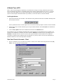
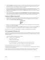
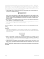
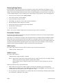
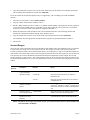
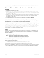
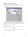
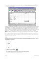
$4XLFN7RXURI)3URIHVVLRQDO
9HUVLRQ
$4XLFN7RXURI)
This is a short tutorial designed to familiarize you with the basic concepts of creating a financial report with F9.
Every F9 financial report starts as a spreadsheet and uses the features of Microsoft Excel or Lotus 1-2-3. For this
reason you will also find Excel’s or Lotus’s online Help to be an invaluable aid when you create your financial
reports. To find complete information about any F9 feature, see the index in the F9 Version 4 Manual.
/HW
VEHJLQWKHWRXU
1.
Open Excel and ensure F9 is attached – there should be an F9 pull-down menu between Window and Help in the
Excel menu list like this:
If the F9 pull-down menu is not listed, please refer to Installation and Setup chapters of the F9 Version 4 Manual.
2.
Ensure that you have a blank workbook open. To open a blank workbook, choose )LOH_1HZ, select Workbook,
and click 2..
3.
Choose 7RROV_2SWLRQV. Select the Calculation tab and click on the 0DQXDO button.
The workbook is now set to Manual Calculation mode. This means that you must instruct Excel to calculate your
formulas. Press the ) key to calculate your entire workbook, 6KLIW) to calculate the active spreadsheet only, or
)(QWHU to calculate the active cell. To save time, all F9 reports should be created with Excel set to Manual
Calculation, so that the entire workbook does not recalculate every time you edit a cell. For more information on
Manual Calculation see the Excel Help under Calculation.
9LHZ<RXU&KDUWRI$FFRXQWV&KDUW
1.
Now we will want to view your Chart of Accounts. To do this, select Chart from the F9 pull-down menu ()_
&KDUW). This will open the F9 Chart window:
$4XLFN7RXURI)
3DJH
2.
Click on the 5HVHW button in the Chart window. Clicking Reset will set the Chart options to be the same as those
specified in F9 Setup. If your company and current year are not listed in the Company and Year dialog boxes,
refer to the Installation and Setup chapters of the F9 User Manual.
3.
Now click the )LQG button. F9 will then run through an Account Match Count. When all the accounts in your GL
have been found you will get a message box stating the number of account keys that were copied to the
Clipboard. Click on the 2. button in this message box and 4XLW the Chart window. This will bring you back to
your blank workbook.
4.
Click on cell A1 and Paste the contents of the clipboard ((GLW_3DVWH). This will fill the spreadsheet with your
basic account information, including your account numbers (column A), descriptions (column B), and balances
for the current open period (column D). The cells may need to be resized to show all of your information.
5HVL]LQJ&HOO:LGWKV8VLQJ$XWR)LW
1.
Select the entire sheet by clicking on the Select All button, which is located at the corner between Row 1 and
Column A. After clicking the Select All button the entire sheet will be highlighted. To AutoFit the column
widths, choose )RUPDW_&ROXPQ_$XWR)LW6HOHFWLRQ.
2.
Rename this spreadsheet GL Formula by double clicking the Sheet1 tab at the bottom left of the Excel window
and typing "GL Formula". Press (QWHU.
3.
Save the workbook as F9 Tour by selecting )LOH_6DYH, typing the File name "F9 Tour", and clicking 6DYH. You
will want to save all F9 Reports often, and always be sure to save a backup copy when it is completed.
Now that we have our Chart of Accounts in Excel, we will want to start learning the basic F9 formulas.
7KH)XQGDPHQWDO))RUPXOD */
The GL Function is the fundamental F9 formula as it links any cell in your spreadsheet to any balance in your general
ledger. This is accomplished with a string of parameters that tell F9 what balance you would like returned. The syntax
of the GL formula is:
=GL(Account, Period, Company, Year, Type, Currency)
Where: Account is the GL Account number
Period is the fiscal period
Company is the specific company
Year is the specific fiscal year
Type is the Account type (i.e. Actual or Budget) that you want this value returned for
Currency is the currency type if your accounting system supports multiple currencies
Write this formula down; in fact write it down twice, as it is the core of all F9 Reports.
The GL formula does not require all 6 parameters, so if your accounting system does not support multiple currencies,
you do not need to enter this specifier.
In many instances you will want your balances to be returned as negative values. To do this, simply use a NGL
function in place of the GL function. The parameters of the NGL function are identical to the GL function.
3DJH
$4XLFN7RXURI)
7KH*/)RUPXOD
1.
Open the F9 Tour workbook, and select the GL Formula sheet if it is not active (click the GL Formula tab).
Cell D4 should contain your first balance. Click on cell D4 and you will see that although there is a value in this
cell there is no formula. The true strength of F9 is rooted in F9 formulas and the ability of all spreadsheets to use
absolute and relative cell references so that they can turn on a single cell.
2.
In cell D4 type the GL formula, substituting the appropriate cell reference for each parameter of the GL formula.
In the example below, as in your sheet, the GL Formula will be:
=GL(A4,D2,A1,B1,C1)
Where: A4 is the Account number
D2 is the Period
A1 is the Company
B1 is the Year
C1 is the Type
3.
ENSURE THAT YOUR CELL REFERENCES ARE CORRECT and press )(QWHU to calculate the cell. If the
formula is correct, the cell will return the same value, but it will now be based on an F9 formula.
As you will notice, none of the other values below cell D4 have changed. This is because they are not formula based.
Don't worry, though; you do not have to type the GL formula again if you use the correct Absolute and Relative cell
references and Auto-Fill.
$EVROXWHDQG5HODWLYH&HOO5HIHUHQFLQJ
By default, a formula you create in Excel uses Relative cell references. This means that if you copy a formula, Excel
will automatically adjust the cell references in the copied formula to refer to different cells, relative to the position of
the original formula. So, if we copy this formula from cell D4 to cell D5, all row references will change by one row.
This formula would then be: =GL(A4,D3,A2,B2,C2).
$4XLFN7RXURI)
3DJH
In the new formula, the Account specifier (A5) is correct but the Period specifier is now cell D3 — which is blank
and obviously not correct. In fact, the Company (A2), Year (B2), and Type (C2) are also incorrect now. To copy this
formula correctly, we will have to ensure that Excel does not adjust the cell references when we copy the formula.
This is called an Absolute reference and is accomplished by placing a dollar sign ($) before the parts of the reference
that do not change. For more information see the Excel Help Index.
1.
Click on cell D4, and in the formula bar (located at the top of the spreadsheet, above the column names) move
your cursor to the Account reference (A4).
2.
Press ). Each time you press F4, Excel toggles through the combinations: absolute column and absolute row
($A$4), relative column and absolute row (A$4), absolute column and relative row ($A4), and relative column
and relative row (A4). We will want the Account reference to change as we copy down rows (relative, no $), but
not across columns (absolute, $). Press ) until the Account reference is $A4. You can also add the $ symbol
with the keyboard.
3.
We will not want the Period reference to change as we copy it down rows, but we will across columns (relative
column and absolute row). Make the Period reference D$2.
4.
The Company, Year, and Type cell references should not change when we copy the formula down or across the
report, so make both the column and row references absolute ($A$1).
5.
Press (QWHU.
The formula should now be: =GL($A4, D$2, $A$1, $B$1, $C$1) and is ready to be copied down all of the account
numbers.
$XWR)LOO
1.
Click on the cell in which the first GL formula is currently specified (D4). You will see a fill handle which is
located at the bottom right of the cell when it is selected. Move your mouse over the fill handle, and your pointer
will become a crosshair.
2.
Double click the fill handle. The formula will now copy down all rows that have a value in Column C. If there is
no value in Column C, or if your version of Excel does not support this feature, simply drag the formula down by
clicking and holding the left mouse button over the fill handle and dragging the formula until the last row with an
account number is selected.
3.
Click on any cell in your spreadsheet. You will notice that all of the cells have the same value as cell D4. This is
because the sheet is set for manual calculation. Press ) to calculate the workbook, and the values from your GL
will populate the report.
Because the Period specifier (cell D2) is currently the word "Month," the values returned are for the current (usually
open) period.
3DJH
$4XLFN7RXURI)
3HULRG6SHFLILHUV
In F9, the Period specifier is used to identify the period or periods for which you are requesting account balances and
uses logical, plain-English terms.
3HULRG6SHFLILHU([DPSOHV 'HVFULSWLRQ
0RQWK
7KHILUVWSHULRGRIWKHILVFDO\HDU
7KLV0RQWK0RQWK
7KHFXUUHQWXVXDOO\RSHQSHULRG
7KLV0RQWK/DVW<HDU
7KHFXUUHQWSHULRGLQWKHSUHYLRXV\HDU
/DVW0RQWK
7KHSHULRGEHIRUHWKHFXUUHQWSHULRG
<HDUWR'DWH<7'
7RWDOIRUWKH\HDULQFOXGLQJWKHFXUUHQWSHULRGDSSOLHVRQO\WR3/DFFRXQWVDV%6DFFRXQWVDUH
UHWXUQHGDVDFXPXODWLYHEDODQFHE\GHIDXOW
&KDQJH0RQWK
3HULRGDFWLYLW\DSSOLHVRQO\WR%6DV3/DFFRXQWVDUHUHWXUQHGDVWUDQVDFWLRQDOYDOXHVE\GHIDXOW
6HSWHPEHU
7KHEDODQFHIRU6HSWHPEHU
4XDUWHU475
7RWDOIRUWKHILUVWTXDUWHU
Let's make the Period specifier January.
1.
Edit cell D2 so that your Period specifier (the second parameter in the GL formula) is January (type "January" in
cell D2).
2.
Recalculate the workbook by pressing the ) key. The values in column D will change to the value of that
account in the month of January (please note, if you are currently posting to January in your GL, this value will
not change).
We will now want to make this report for multiple periods. Fortunately, we do not have to manually enter each month
in the appropriate cell as Excel has the ability to generate data automatically based on the data in the original cell.
This is referred to as a copy series.
1.
Select cell D2 (January).
2.
Move your mouse over the fill handle and your pointer will become a crosshair. Press and hold the left mouse
button and drag the selected cell across columns until it covers all the periods between January and December
(stop at Column O).
3.
Select cell D4, and copy the formula across all of the periods.
4.
To copy the formula down, select only cells E4 through O4 and double click the fill handle. If the D column is
selected this will not work because D5 already has a formula in it.
5.
Press ) to calculate the report. This may take a few minutes if you have a large Chart of Accounts.
6.
Select the entire Sheet and AutoFit the selection.
7.
Save the workbook ()LOH_6DYH).
You may notice that your Balance Sheet accounts have the same value for a consecutive number of periods (current
period and all future periods). F9, following the principles of accounting, returns Balance Sheet accounts as a
cumulative balance. P/L accounts are returned as a monthly change value.
$4XLFN7RXURI)
3DJH
5HWXUQLQJ%XGJHW9DOXHV
To return budget values in F9, use the same GL Formula as for Actual values but add the word "Budget" to your
Period specifier. All valid Period specifiers can be used to return budget values. So a period parameter of "January
Budget" will return the budgeted amount for that account. Then add a BUDGET type specifier to the Control Area. If
you have multiple budgets in your accounting system, simply change the Type specifier to the correct budget name.
1.
Select any cell in Column E. Choose ,QVHUW_&ROXPQ.
2.
Select cell E2 and enter "January Budget".
3.
Copy the formula in cell D4 to cell E4.
4.
Add a Budget Type Specifier. Select cell E1 and enter "BUDGET".
5.
Edit the formula in cell E4. Change $C$1 to $E$1.
6.
Auto-Fill the formula in cell E4 down all account numbers.
7.
Recalculate the workbook (F9).
8.
Save the workbook.
That's it. You now have January's budget values for the specified Type (cell E1) in Column E.
'HVFULSWLRQ)RUPXODV
We will now want to make the descriptions in this report formula-based so that when you edit an account number it
will return the appropriate description.
In F9 there are two formulas for returning account descriptions, these are the DESC Function and SDESC Function.
DESC returns the account description for the full account code. If the DESC function is used on a range or list of
accounts, it returns the appropriate description for the first account number in the range or list. SDESC produces the
descriptions associated with the individual segments of the account code. In short, the DESC is used to return the
Natural Account description and SDESC is used to return the Sub-Account description.
'(6&)XQFWLRQ
The syntax of this formula is the same as the GL function except it omits the Period specifier:
=DESC(Account, Company, Year)
6'(6&)XQFWLRQ
The syntax of this formula is:
=SDESC(Segment, Segment Number, Company)
Where: Segment may contain either a single segment value or a complete account code. If a complete account
number is provided, the single segment is extracted and evaluated.
Segment Number always contains the number of the segment you wish a description for. The first
segment is "1."
Make the descriptions in this report formula based:
1.
Make cell B4 active and enter the =DESC formula, referencing the appropriate cells for each parameter
[=DESC(Account, Company, Year)]. Press (QWHU and recalculate this cell ()(QWHU). If the description is not
returned ensure that your formula is correct i.e. =DESC(A4, A1,B1).
2.
Give the parameters in this formula the correct absolute and relative cell referencing. The DESC function should
now be defined as: =DESC($A4, $A$1, $B$1).
3DJH
$4XLFN7RXURI)
3.
Copy the formula down so that it covers all accounts. Ensure that you entered the correct absolute and relative
cell referencing and recalculate the current sheet (6KLIW)).
F9 can also return sub-account descriptions if they are supported by your accounting system with the SDESC
function.
1.
Select any cell in Column C. Choose ,QVHUW_&ROXPQ.
2.
Copy the =DESC function from Cell B4 to Cell C4.
3.
Edit the =DESC formula in Cell C3 so that it is a =SDESC formula, pulling a description for the first segment of
your account code [=SDESC($A4,"1",$A$1,$B$1)]. If the first segment of your account code is your natural
account you will want to return a description for a segment other than "1".
4.
Ensure the parameters in this formula have the correct absolute and relative cell referencing. Because this
formula was copied from the DESC formula, these should be correct.
5.
Copy the formula down so that it covers all accounts, and recalculate the current sheet (6KLIW)).
You should now have the appropriate description for the segment you specified returned in Column C.
6.
Save the File.
$FFRXQW5DQJHV
So far, the only values returned have been for individual account numbers, but in most financial reports you will want
to return values for a range or series of accounts in one cell. For example, to return a value for all of your cash
accounts (a Natural Account code of 10005 through 10030), you would specify a range of accounts that includes all
cash accounts. Let's assume that you have a three-segment account code where the first segment of your account code
is the Location, the second is the Natural Account and the third is the Department. In this example, the Account
specifier would be *-10005..10030-*. This would return the value for all accounts between 10005 and 10030 for all
Locations and all Departments. As you can see, Wildcards (the asterisk), can be used in specifying ranges of accounts
with F9.
$FFRXQW
6SHFLILHU
"
'HVFULSWLRQ
([DPSOH
0DWFKHVDQ\FKDUDFWHU RUVHWRIFKDUDFWHUV
UHJDUGOHVVRIOHQJWK
0DWFKHVDVLQJOH
FKDUDFWHULQWKHH[DFW
SRVLWLRQ
5HVXOW
5HWXUQVDOODFFRXQWVDOOGHSDUWPHQWVDOOORFDWLRQV
5HWXUQVWKHDFFRXQWVIRUDOO/RFDWLRQVLQ
'HSDUWPHQW
$
5HWXUQVDOODFFRXQWVWKDWVWDUWZLWKDIRU/RFDWLRQ$
DQG'HSDUWPHQW
$"
5HWXUQVDOODFFRXQWVWKDWKDYHDVWKHLUVWFKDUDFWHU
DVWKHLUQGFKDUDFWHUDVWKHLUUGFKDUDFWHUDQG
DVWKHLUILQDOFKDUDFWHUIRU/RFDWLRQ$DQG'HSDUWPHQW
,QGLFDWHVDUDQJHRI
DFFRXQWVHJPHQWYDOXHV
5HWXUQVDOODFFRXQWVIURPXSWRDQGLQFOXGLQJ
IRUDOO/RFDWLRQVDQGDOO'HSDUWPHQWV
&UHDWHVDOLVWRIDFFRXQW $
VSHFLILHUVRUDFFRXQW
VHJPHQWV
5HWXUQVDEDODQFHIRUWKHVXPRIDFFRXQW$
DQGZLWKDOO/RFDWLRQVDQGDOO'HSDUWPHQWV
3OHDVHQRWHWKDWIRUPRVWUDQJHVRIDFFRXQWVWRZRUN\RXPXVWKDYH5HWXUQ=HUR)RU$FFRXQW0DWFK1RW
)RXQGVHOHFWHGLQ)6HWXS
$4XLFN7RXURI)
3DJH
Let's add a line to the report that pulls the value for all Balance Sheet accounts and a line that pulls the value for all
Profit and Loss accounts.
5HWXUQLQJD%DODQFHIRU$OO%DODQFH6KHHW$FFRXQWVDQG$OO3URILWDQG/RVV
$FFRXQWV
1.
Scroll down to the last line of your report.
2.
In the first empty A cell, enter the appropriate account range for all Balance Sheet accounts. In most cases the
Natural Account range would be 10000..39999, with an asterisk for all sub-accounts. In this example, the Natural
Account range is 10000..29999.
3.
In the next A cell, enter the appropriate account range for all Profit and Loss accounts. In most cases the Natural
Account range would be 40000..99999, with an asterisk for all sub-accounts. In this example, the Natural
Account range is 30000..99999.
4.
Copy the formulas from the above row to these rows, and calculate the current sheet (6KLIW)).
The descriptions for these ranges will not signify the fact that this is a range of accounts and will return the
description for the first account listed. If you have a number of ranges of accounts that you will be using frequently,
the best thing to do is create Financial Entities in F9 for these ranges. For information on Financial Entities and other
advanced F9 features, see the F9 User Manual, or consider registering for F9 Training.
Although these Account specifiers may seem to be able to accommodate every aspect of your reporting needs,
imagine if you wanted to create a departmentalized report for each department. Using the above Account ranges will
accomplish this, but you will have to recreate the report for each department, reentering the appropriate account
ranges, each time specifying a different department. A very important feature of F9 is allowing you to cell reference
each segment of your account code individually, so that you can make your report turn on any segment of your
account code. This is accomplished with the BSPEC Function.
%63(&
The BSPEC function expands the functionality of the Account specifier by Building the Account SPECifiers from
cell references. The BSPEC is really just the Account parameter in any F9 formula that uses an Account parameter.
The Syntax of the BSPEC is:
=BSPEC(Segment 1, Segment 2, Segment 3)
Where: Segment 1 is a cell reference to the first segment of your account
Segment 2 is a cell reference to the second segment of your account
Segment 3 is a cell reference to the third segment of your account
There can be as many Segments as your account contains.
The GL formula with the BSPEC function:
=GL(BSPEC(Segment 1, Segment 2, Segment 3),Period, Company, Year, Type)
In any F9 formula that references an account number, the BSPEC can also be a cell reference.
The easiest way to learn the BSPEC function is to see it in use. The F9 report that we have created is not really suited
to using the BSPEC function. We will now go to Sheet 2 and create a departmentalized Profit and Loss statement.
3DJH
$4XLFN7RXURI)
7KH*/:L]DUG$FFRXQW(QTXLUHDQG*/3DVWH
The GL Wizard creates the first GL formula in a new report using the BSPEC function, which reduces the time to
create reports because it enters the correct absolute and relative cell referencing.
1.
Click on the Sheet 2 Page Tab at the bottom of the spreadsheet to make Sheet 2 active. Double click the Tab, and
rename this sheet BSPEC.
2.
Choose )_(QTXLUH. This will open the F9 Account Enquire window.
3.
Using the drop-down lists, complete the specifics of the GL Function. That is the Account by Company
Identifier, Periods, Type, Segments, and Year. The &UHDWH*/)XQFWLRQ%\ option determines which GL
parameter becomes the horizontal axis on your report. In most cases this will be Period. Be sure to select as the
Natural Account the first P/L account that you know has a balance. Leave the other account segments as asterisk
(ALL).
4.
Click *HW%DODQFH to return the balance of the selected account(s).
5.
Click 4XLW.
Now to paste the GL Formula into the spreadsheet we will use GL Paste. GL Paste interprets the information from the
Account Enquiry to form a valid GL Function.
1.
Select cell A1 in the BSPEC spreadsheet and click the GL Paste toolbar button. The formula, as well as the
Control Area for your report, is pasted into the spreadsheet.
$4XLFN7RXURI)
3DJH
2.
Select the entire sheet and Auto-Fit the column widths. Choose )RUPDW_&ROXPQ_$XWR)LW6HOHFWLRQ. Your
sheet will now look similar to:
In the above sample cell E10 contains the value for the account(s) that was specified in Account Enquire. If you click
on the appropriate cell in your sheet you will see that there is a GL formula with the proper BSPEC function and
absolute and relative cell referencing. In the sample sheet above, the BSPEC references cell B1 (Location), A10
(Natural Account) and B3 (Department). Currently the Location and Department segments are referencing an asterisk
meaning 'ALL'. To reference a specific department, location, sub-account, division, region, etc., change the
appropriate reference to the department or location that you will want the sheet for, and recalculate cell E10 (6KLIW
)).
Now, the sheet has only one account referenced. You can begin entering Natural Account codes and ranges in cell
A11, A12, etc. If you do not want to consolidate any accounts, the fastest way to output the entities that exist in any
segment of your account code is Lists.
/LVWV
The primary role of the Lists feature is to save time manually entering data that already exists in your GL. The List
feature allows you to enumerate:
1.
•
Segments
•
Companies
•
Budgets
•
Lists
•
Periods
•
Years
Click the Lists Toolbar Button.
The Available Lists section allows you to select the List that will be generated.
List Segment: determines which segment will be listed
3DJH
$4XLFN7RXURI)
Where: defines the limitation that you will define in the Is: section.
Is: determines the limitation on the List output, i.e. an Account range (only for P/L accounts). Wildcards and
ranges can be used.
Transpose List: generates the List on the horizontal axis if selected (usually selected for Period specifiers).
Generate Descriptions: creates descriptions, if available, for the selected segment (not formula based).
2.
Select Segments under Available Lists.
3.
Select the following:
4.
•
In the List Segment drop-down, select Account
•
In the Where drop-down, select Account
•
In the Is field, type 30100..80500 or the appropriate range for all of your P/L Accounts
Click 6HQG7R&OLSERDUGpress 2. to the List was Sent To Clipboard message, and 4XLW the Lists window.
Now that the List of all of your P/L Accounts has been sent to the Clipboard we will want to paste this into the
BSPEC sheet and finish the report.
1.
Select the cell in the BSPEC sheet that contains your first account number (Cell A10 in the above Example) and
select Paste ((GLW_3DVWH). This will paste in all P/L Natural Account codes.
2.
Click on the NGL formula and copy the formula down so that it covers all account numbers.
3.
Copy the first NGL formula and paste it to the corresponding Row in Column B and edit the formula so that it is
a DSEC formula. That is, change NGL to DESC then delete the Period specifier. Your Description formula will
now be similar to: =DESC(BSPEC($B$1,$A10,$B$3),$B$5,$B$6).
4.
Copy the DESC formula across all account numbers.
5.
Recalculate the report.
6.
AutoFit and Save the report.
You have now completed the beginning of your Departmentalized P/L Statement. To change the Location (or
Department, etc.), simply edit the appropriate cell on the sheet (cells B1and B3 in the sample) and recalculate. To
change the Period, simply edit the Period specifier. If you like, make this a multiple period report by adding Periods.
$4XLFN7RXURI)
3DJH
You can use the features of Excel and F9 to make this report exactly how you would envision the ideal P/L Report.
Add sum lines, change single account specifiers to ranges, add a variance column to compare the current year versus
the past year, make graphs and charts, add macros, etc. These are all benefits of creating your financial reports with
F9 in a spreadsheet program as powerful as Excel.
For more information and for detailed instructions on the advanced features of F9, please see your F9 Version 4
Manual.
3DJH
$4XLFN7RXURI)