Download Spectre Circuit Simulator User Guide

Spectre Circuit Simulator User Guide
Product Version 5.0
January 2004
 1990-2003 Cadence Design Systems, Inc. All rights reserved.
Printed in the United States of America.
Cadence Design Systems, Inc., 555 River Oaks Parkway, San Jose, CA 95134, USA
Trademarks: Trademarks and service marks of Cadence Design Systems, Inc. (Cadence) contained in
this document are attributed to Cadence with the appropriate symbol. For queries regarding Cadence’s
trademarks, contact the corporate legal department at the address shown above or call 800.862.4522.
All other trademarks are the property of their respective holders.
Restricted Print Permission: This publication is protected by copyright and any unauthorized use of this
publication may violate copyright, trademark, and other laws. Except as specified in this permission
statement, this publication may not be copied, reproduced, modified, published, uploaded, posted,
transmitted, or distributed in any way, without prior written permission from Cadence. This statement grants
you permission to print one (1) hard copy of this publication subject to the following conditions:
1. The publication may be used solely for personal, informational, and noncommercial purposes;
2. The publication may not be modified in any way;
3. Any copy of the publication or portion thereof must include all original copyright, trademark, and other
proprietary notices and this permission statement; and
4. Cadence reserves the right to revoke this authorization at any time, and any such use shall be
discontinued immediately upon written notice from Cadence.
Disclaimer: Information in this publication is subject to change without notice and does not represent a
commitment on the part of Cadence. The information contained herein is the proprietary and confidential
information of Cadence or its licensors, and is supplied subject to, and may be used only by Cadence’s
customer in accordance with, a written agreement between Cadence and its customer. Except as may be
explicitly set forth in such agreement, Cadence does not make, and expressly disclaims, any
representations or warranties as to the completeness, accuracy or usefulness of the information contained
in this document. Cadence does not warrant that use of such information will not infringe any third party
rights, nor does Cadence assume any liability for damages or costs of any kind that may result from use of
such information.
Restricted Rights: Use, duplication, or disclosure by the Government is subject to restrictions as set forth
in FAR52.227-14 and DFAR252.227-7013 et seq. or its successor.
Spectre Circuit Simulator User Guide
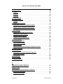
Contents
Preface . . . . . . . . . . . . . . . . . . . . . . . . . . . . . . . . . . . . . . . . . . . . . . . . . . . . . . . . . . . . . 13
Related Documents . . . . . . . . . . . . . . . . . . . . . . . . . . . . . . . . . . . . . . . . . . . . . . . . . . . . . 13
Typographic and Syntax Conventions . . . . . . . . . . . . . . . . . . . . . . . . . . . . . . . . . . . . . . . 14
References . . . . . . . . . . . . . . . . . . . . . . . . . . . . . . . . . . . . . . . . . . . . . . . . . . . . . . . . . . . . 15
1
Introducing the Spectre Circuit Simulator . . . . . . . . . . . . . . . . . . . . . . 16
Improvements over SPICE . . . . . . . . . . . . . . . . . . . . . . . . . . . . . . . . . . . . . . . . . . . . . . . .
Improved Capacity . . . . . . . . . . . . . . . . . . . . . . . . . . . . . . . . . . . . . . . . . . . . . . . . . . .
Improved Accuracy . . . . . . . . . . . . . . . . . . . . . . . . . . . . . . . . . . . . . . . . . . . . . . . . . . .
Improved Speed . . . . . . . . . . . . . . . . . . . . . . . . . . . . . . . . . . . . . . . . . . . . . . . . . . . . .
Improved Reliability . . . . . . . . . . . . . . . . . . . . . . . . . . . . . . . . . . . . . . . . . . . . . . . . . .
Improved Models . . . . . . . . . . . . . . . . . . . . . . . . . . . . . . . . . . . . . . . . . . . . . . . . . . . .
Spectre Usability Features and Customer Service . . . . . . . . . . . . . . . . . . . . . . . . . . .
Analog HDLs . . . . . . . . . . . . . . . . . . . . . . . . . . . . . . . . . . . . . . . . . . . . . . . . . . . . . . . . . .
RF Capabilities . . . . . . . . . . . . . . . . . . . . . . . . . . . . . . . . . . . . . . . . . . . . . . . . . . . . . . . .
Mixed-Signal Simulation . . . . . . . . . . . . . . . . . . . . . . . . . . . . . . . . . . . . . . . . . . . . . . . . .
Environments . . . . . . . . . . . . . . . . . . . . . . . . . . . . . . . . . . . . . . . . . . . . . . . . . . . . . . . . . .
17
17
17
18
19
20
20
21
21
23
23
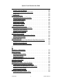
2
Getting Started with Spectre . . . . . . . . . . . . . . . . . . . . . . . . . . . . . . . . . . . . 25
Using the Example and Displaying Results . . . . . . . . . . . . . . . . . . . . . . . . . . . . . . . . . . .
Sample Schematic . . . . . . . . . . . . . . . . . . . . . . . . . . . . . . . . . . . . . . . . . . . . . . . . . . . . . .
Sample Netlist . . . . . . . . . . . . . . . . . . . . . . . . . . . . . . . . . . . . . . . . . . . . . . . . . . . . . . . . .
Elements of a Spectre Netlist . . . . . . . . . . . . . . . . . . . . . . . . . . . . . . . . . . . . . . . . . . .
Instructions for a Spectre Simulation Run . . . . . . . . . . . . . . . . . . . . . . . . . . . . . . . . . . . .
Following Simulation Progress . . . . . . . . . . . . . . . . . . . . . . . . . . . . . . . . . . . . . . . . . .
Screen Printout . . . . . . . . . . . . . . . . . . . . . . . . . . . . . . . . . . . . . . . . . . . . . . . . . . . . . .
Viewing Your Output . . . . . . . . . . . . . . . . . . . . . . . . . . . . . . . . . . . . . . . . . . . . . . . . . . . .
Starting WaveScan . . . . . . . . . . . . . . . . . . . . . . . . . . . . . . . . . . . . . . . . . . . . . . . . . . .
January 2004
3
26
26
28
29
32
33
33
34
34
Product Version 5.0
Spectre Circuit Simulator User Guide
Plotting Signals . . . . . . . . . . . . . . . . . . . . . . . . . . . . . . . . . . . . . . . . . . . . . . . . . . . . . . 35
Changing the Trace Color . . . . . . . . . . . . . . . . . . . . . . . . . . . . . . . . . . . . . . . . . . . . . . 37
Learning More about WaveScan . . . . . . . . . . . . . . . . . . . . . . . . . . . . . . . . . . . . . . . . 38
3
SPICE Compatibility . . . . . . . . . . . . . . . . . . . . . . . . . . . . . . . . . . . . . . . . . . . . . . 41
Reading SPICE Netlists . . . . . . . . . . . . . . . . . . . . . . . . . . . . . . . . . . . . . . . . . . . . . . . . . .
Running the SPICE Reader . . . . . . . . . . . . . . . . . . . . . . . . . . . . . . . . . . . . . . . . . . . .
Running the SPICE Reader from Cadence Analog Design Environment . . . . . . . . .
Running the SPICE Reader from the Command Line . . . . . . . . . . . . . . . . . . . . . . . .
Using the SPICE Reader to Convert Netlists . . . . . . . . . . . . . . . . . . . . . . . . . . . . . . .
Language Differences . . . . . . . . . . . . . . . . . . . . . . . . . . . . . . . . . . . . . . . . . . . . . . . . . . .
Comparing the SPICE and Spectre Languages . . . . . . . . . . . . . . . . . . . . . . . . . . . . .
Reading SPICE and Spectre Files . . . . . . . . . . . . . . . . . . . . . . . . . . . . . . . . . . . . . . .
Scope of the Compatibility . . . . . . . . . . . . . . . . . . . . . . . . . . . . . . . . . . . . . . . . . . . . . . . .
Sources . . . . . . . . . . . . . . . . . . . . . . . . . . . . . . . . . . . . . . . . . . . . . . . . . . . . . . . . . . .
Compatibility Guidelines . . . . . . . . . . . . . . . . . . . . . . . . . . . . . . . . . . . . . . . . . . . . . . .
General Input Compatibility . . . . . . . . . . . . . . . . . . . . . . . . . . . . . . . . . . . . . . . . . . . .
Compatibility Limitations . . . . . . . . . . . . . . . . . . . . . . . . . . . . . . . . . . . . . . . . . . . . . . .
42
42
43
43
44
48
48
50
51
51
51
51
55
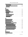
4
Spectre Netlists . . . . . . . . . . . . . . . . . . . . . . . . . . . . . . . . . . . . . . . . . . . . . . . . . . . 57
Netlist Statements . . . . . . . . . . . . . . . . . . . . . . . . . . . . . . . . . . . . . . . . . . . . . . . . . . . . . .
Netlist Conventions . . . . . . . . . . . . . . . . . . . . . . . . . . . . . . . . . . . . . . . . . . . . . . . . . . .
Basic Syntax Rules . . . . . . . . . . . . . . . . . . . . . . . . . . . . . . . . . . . . . . . . . . . . . . . . . .
Spectre Language Modes . . . . . . . . . . . . . . . . . . . . . . . . . . . . . . . . . . . . . . . . . . . . .
Creating Component and Node Names . . . . . . . . . . . . . . . . . . . . . . . . . . . . . . . . . . .
Escaping Special Characters in Names . . . . . . . . . . . . . . . . . . . . . . . . . . . . . . . . . . .
Instance Statements . . . . . . . . . . . . . . . . . . . . . . . . . . . . . . . . . . . . . . . . . . . . . . . . . . . .
Formatting the Instance Statement . . . . . . . . . . . . . . . . . . . . . . . . . . . . . . . . . . . . . .
Examples of Instance Statements . . . . . . . . . . . . . . . . . . . . . . . . . . . . . . . . . . . . . . .
Basic Instance Statement Rules . . . . . . . . . . . . . . . . . . . . . . . . . . . . . . . . . . . . . . . .
Identical Components or Subcircuits in Parallel . . . . . . . . . . . . . . . . . . . . . . . . . . . . .
Analysis Statements . . . . . . . . . . . . . . . . . . . . . . . . . . . . . . . . . . . . . . . . . . . . . . . . . . . .
Basic Formatting of Analysis Statements . . . . . . . . . . . . . . . . . . . . . . . . . . . . . . . . . .
January 2004
4
58
58
59
59
60
62
62
62
64
64
65
66
66
Product Version 5.0
Spectre Circuit Simulator User Guide
Examples of Analysis Statements . . . . . . . . . . . . . . . . . . . . . . . . . . . . . . . . . . . . . . .
Basic Analysis Rules . . . . . . . . . . . . . . . . . . . . . . . . . . . . . . . . . . . . . . . . . . . . . . . . .
Control Statements . . . . . . . . . . . . . . . . . . . . . . . . . . . . . . . . . . . . . . . . . . . . . . . . . . . . .
Formatting the Control Statement . . . . . . . . . . . . . . . . . . . . . . . . . . . . . . . . . . . . . . .
Examples of Control Statements . . . . . . . . . . . . . . . . . . . . . . . . . . . . . . . . . . . . . . . .
Model Statements . . . . . . . . . . . . . . . . . . . . . . . . . . . . . . . . . . . . . . . . . . . . . . . . . . . . . .
Formatting the model Statement . . . . . . . . . . . . . . . . . . . . . . . . . . . . . . . . . . . . . . . .
Examples of model Statements . . . . . . . . . . . . . . . . . . . . . . . . . . . . . . . . . . . . . . . . .
Basic model Statement Rules . . . . . . . . . . . . . . . . . . . . . . . . . . . . . . . . . . . . . . . . . .
Input Data from Multiple Files . . . . . . . . . . . . . . . . . . . . . . . . . . . . . . . . . . . . . . . . . . . . .
Formatting the include Statement . . . . . . . . . . . . . . . . . . . . . . . . . . . . . . . . . . . . . . .
Rules for Using the include Statement . . . . . . . . . . . . . . . . . . . . . . . . . . . . . . . . . . . .
Example of include Statement Use . . . . . . . . . . . . . . . . . . . . . . . . . . . . . . . . . . . . . .
Reading Piecewise Linear (PWL) Vector Values from a File . . . . . . . . . . . . . . . . . . .
Using Library Statements . . . . . . . . . . . . . . . . . . . . . . . . . . . . . . . . . . . . . . . . . . . . . .
Multidisciplinary Modeling . . . . . . . . . . . . . . . . . . . . . . . . . . . . . . . . . . . . . . . . . . . . . . . .
Setting Tolerances with the quantity Statement . . . . . . . . . . . . . . . . . . . . . . . . . . . . .
Inherited Connections . . . . . . . . . . . . . . . . . . . . . . . . . . . . . . . . . . . . . . . . . . . . . . . . . . .
67
68
68
69
69
70
71
71
72
72
72
73
74
74
75
76
76
78
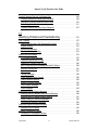
5
Parameter Specification and Modeling Features . . . . . . . . . . . . . 79
Instance (Component or Analysis) Parameters . . . . . . . . . . . . . . . . . . . . . . . . . . . . . . . .
Types of Parameter Values . . . . . . . . . . . . . . . . . . . . . . . . . . . . . . . . . . . . . . . . . . . . .
Parameter Dimension . . . . . . . . . . . . . . . . . . . . . . . . . . . . . . . . . . . . . . . . . . . . . . . . .
Parameter Ranges . . . . . . . . . . . . . . . . . . . . . . . . . . . . . . . . . . . . . . . . . . . . . . . . . . .
Help on Parameters . . . . . . . . . . . . . . . . . . . . . . . . . . . . . . . . . . . . . . . . . . . . . . . . . .
Scaling Numerical Literals . . . . . . . . . . . . . . . . . . . . . . . . . . . . . . . . . . . . . . . . . . . . .
Parameters Statement . . . . . . . . . . . . . . . . . . . . . . . . . . . . . . . . . . . . . . . . . . . . . . . . . . .
Circuit and Subcircuit Parameters . . . . . . . . . . . . . . . . . . . . . . . . . . . . . . . . . . . . . . .
Parameter Declaration . . . . . . . . . . . . . . . . . . . . . . . . . . . . . . . . . . . . . . . . . . . . . . . .
Parameter Inheritance . . . . . . . . . . . . . . . . . . . . . . . . . . . . . . . . . . . . . . . . . . . . . . . .
Parameter Referencing . . . . . . . . . . . . . . . . . . . . . . . . . . . . . . . . . . . . . . . . . . . . . . . .
Altering/Sweeping Parameters . . . . . . . . . . . . . . . . . . . . . . . . . . . . . . . . . . . . . . . . . .
Expressions . . . . . . . . . . . . . . . . . . . . . . . . . . . . . . . . . . . . . . . . . . . . . . . . . . . . . . . . . . .
Behavioral Expressions . . . . . . . . . . . . . . . . . . . . . . . . . . . . . . . . . . . . . . . . . . . . . . .
January 2004
5
80
80
80
81
82
83
84
85
85
85
86
86
86
90
Product Version 5.0
Spectre Circuit Simulator User Guide
Built-in Constants . . . . . . . . . . . . . . . . . . . . . . . . . . . . . . . . . . . . . . . . . . . . . . . . . . . . 91
User-Defined Functions . . . . . . . . . . . . . . . . . . . . . . . . . . . . . . . . . . . . . . . . . . . . . . . 92
Predefined Netlist Parameters . . . . . . . . . . . . . . . . . . . . . . . . . . . . . . . . . . . . . . . . . . 93
Subcircuits . . . . . . . . . . . . . . . . . . . . . . . . . . . . . . . . . . . . . . . . . . . . . . . . . . . . . . . . . . . . 93
Formatting Subcircuit Definitions . . . . . . . . . . . . . . . . . . . . . . . . . . . . . . . . . . . . . . . . 94
A Subcircuit Definition Example . . . . . . . . . . . . . . . . . . . . . . . . . . . . . . . . . . . . . . . . . 94
Subcircuit Example . . . . . . . . . . . . . . . . . . . . . . . . . . . . . . . . . . . . . . . . . . . . . . . . . . . 95
Rules to Remember . . . . . . . . . . . . . . . . . . . . . . . . . . . . . . . . . . . . . . . . . . . . . . . . . . 96
Calling Subcircuits . . . . . . . . . . . . . . . . . . . . . . . . . . . . . . . . . . . . . . . . . . . . . . . . . . . 97
Modifying Subcircuit Parameter Values . . . . . . . . . . . . . . . . . . . . . . . . . . . . . . . . . . . 98
Checking for Invalid Parameter Values . . . . . . . . . . . . . . . . . . . . . . . . . . . . . . . . . . . . 98
Inline Subcircuits . . . . . . . . . . . . . . . . . . . . . . . . . . . . . . . . . . . . . . . . . . . . . . . . . . . . . . . 99
Modeling Parasitics . . . . . . . . . . . . . . . . . . . . . . . . . . . . . . . . . . . . . . . . . . . . . . . . . 100
Parameterized Models . . . . . . . . . . . . . . . . . . . . . . . . . . . . . . . . . . . . . . . . . . . . . . . 102
Inline Subcircuits Containing Only Inline model Statements . . . . . . . . . . . . . . . . . . 103
Process Modeling Using Inline Subcircuits . . . . . . . . . . . . . . . . . . . . . . . . . . . . . . . 104
Binning . . . . . . . . . . . . . . . . . . . . . . . . . . . . . . . . . . . . . . . . . . . . . . . . . . . . . . . . . . . . . . 107
Auto Model Selection . . . . . . . . . . . . . . . . . . . . . . . . . . . . . . . . . . . . . . . . . . . . . . . . 108
Conditional Instances . . . . . . . . . . . . . . . . . . . . . . . . . . . . . . . . . . . . . . . . . . . . . . . . 109
Scaling Physical Dimensions of Components . . . . . . . . . . . . . . . . . . . . . . . . . . . . . . . . 118
N-Ports . . . . . . . . . . . . . . . . . . . . . . . . . . . . . . . . . . . . . . . . . . . . . . . . . . . . . . . . . . . . . . 120
N-Port Example . . . . . . . . . . . . . . . . . . . . . . . . . . . . . . . . . . . . . . . . . . . . . . . . . . . . 120
Creating an S-Parameter File Automatically . . . . . . . . . . . . . . . . . . . . . . . . . . . . . . . 121
Creating an S, Y, or Z-Parameter File Manually . . . . . . . . . . . . . . . . . . . . . . . . . . . . 121
Reading the S, Y or Z-Parameter File . . . . . . . . . . . . . . . . . . . . . . . . . . . . . . . . . . . 122
Touchstone Format . . . . . . . . . . . . . . . . . . . . . . . . . . . . . . . . . . . . . . . . . . . . . . . . . . 124
S-Parameter File Format Translator . . . . . . . . . . . . . . . . . . . . . . . . . . . . . . . . . . . . . 128
6
Analyses . . . . . . . . . . . . . . . . . . . . . . . . . . . . . . . . . . . . . . . . . . . . . . . . . . . . . . . . . . 130
Types of Analyses . . . . . . . . . . . . . . . . . . . . . . . . . . . . . . . . . . . . . . . . . . . . . . . . . . . . .
Analysis Parameters . . . . . . . . . . . . . . . . . . . . . . . . . . . . . . . . . . . . . . . . . . . . . . . . . . .
Probes in Analyses . . . . . . . . . . . . . . . . . . . . . . . . . . . . . . . . . . . . . . . . . . . . . . . . . . . .
Multiple Analyses . . . . . . . . . . . . . . . . . . . . . . . . . . . . . . . . . . . . . . . . . . . . . . . . . . . . . .
Multiple Analyses in a Subcircuit . . . . . . . . . . . . . . . . . . . . . . . . . . . . . . . . . . . . . . . . . .
January 2004
6
131
134
135
135
138
Product Version 5.0
Spectre Circuit Simulator User Guide
Example . . . . . . . . . . . . . . . . . . . . . . . . . . . . . . . . . . . . . . . . . . . . . . . . . . . . . . . . . .
DC Analysis . . . . . . . . . . . . . . . . . . . . . . . . . . . . . . . . . . . . . . . . . . . . . . . . . . . . . . . . . .
AC Analysis . . . . . . . . . . . . . . . . . . . . . . . . . . . . . . . . . . . . . . . . . . . . . . . . . . . . . . . . . .
Transient Analysis . . . . . . . . . . . . . . . . . . . . . . . . . . . . . . . . . . . . . . . . . . . . . . . . . . . . .
Trading Off Speed and Accuracy with a Single Parameter Setting . . . . . . . . . . . . . .
Controlling the Accuracy . . . . . . . . . . . . . . . . . . . . . . . . . . . . . . . . . . . . . . . . . . . . .
Setting the Integration Method . . . . . . . . . . . . . . . . . . . . . . . . . . . . . . . . . . . . . . . . .
Improving Transient Analysis Convergence . . . . . . . . . . . . . . . . . . . . . . . . . . . . . . .
Controlling the Amount of Output Data . . . . . . . . . . . . . . . . . . . . . . . . . . . . . . . . . .
Pole Zero Analysis . . . . . . . . . . . . . . . . . . . . . . . . . . . . . . . . . . . . . . . . . . . . . . . . . . . . .
Syntax . . . . . . . . . . . . . . . . . . . . . . . . . . . . . . . . . . . . . . . . . . . . . . . . . . . . . . . . . . .
Example 1 . . . . . . . . . . . . . . . . . . . . . . . . . . . . . . . . . . . . . . . . . . . . . . . . . . . . . . . .
Example 2 . . . . . . . . . . . . . . . . . . . . . . . . . . . . . . . . . . . . . . . . . . . . . . . . . . . . . . . .
Example 3 . . . . . . . . . . . . . . . . . . . . . . . . . . . . . . . . . . . . . . . . . . . . . . . . . . . . . . . .
Output Log File . . . . . . . . . . . . . . . . . . . . . . . . . . . . . . . . . . . . . . . . . . . . . . . . . . . . .
Other Analyses (sens, fourier, dcmatch, and stb) . . . . . . . . . . . . . . . . . . . . . . . . . . . . .
Sensitivity Analysis . . . . . . . . . . . . . . . . . . . . . . . . . . . . . . . . . . . . . . . . . . . . . . . . . .
Fourier Analysis . . . . . . . . . . . . . . . . . . . . . . . . . . . . . . . . . . . . . . . . . . . . . . . . . . . .
DC Match Analysis . . . . . . . . . . . . . . . . . . . . . . . . . . . . . . . . . . . . . . . . . . . . . . . . . .
Stability Analysis . . . . . . . . . . . . . . . . . . . . . . . . . . . . . . . . . . . . . . . . . . . . . . . . . . .
Advanced Analyses (sweep and montecarlo) . . . . . . . . . . . . . . . . . . . . . . . . . . . . . . . .
Sweep Analysis . . . . . . . . . . . . . . . . . . . . . . . . . . . . . . . . . . . . . . . . . . . . . . . . . . . .
Monte Carlo Analysis . . . . . . . . . . . . . . . . . . . . . . . . . . . . . . . . . . . . . . . . . . . . . . . .
Special Analysis (Hot-Electron Degradation) . . . . . . . . . . . . . . . . . . . . . . . . . . . . . . . . .
Hot-Electron Degradation Analysis . . . . . . . . . . . . . . . . . . . . . . . . . . . . . . . . . . . . . .
Output Options for Hot-Electron Degradation Analysis . . . . . . . . . . . . . . . . . . . . . .
Example of Hot-Electron Degradation . . . . . . . . . . . . . . . . . . . . . . . . . . . . . . . . . . .
138
139
140
141
142
143
144
145
145
148
149
149
149
149
150
150
151
153
154
157
159
159
164
178
179
180
181
7
Control Statements . . . . . . . . . . . . . . . . . . . . . . . . . . . . . . . . . . . . . . . . . . . . . . 186
The alter and altergroup Statements . . . . . . . . . . . . . . . . . . . . . . . . . . . . . . . . . . . . . . .
Changing Parameter Values for Components . . . . . . . . . . . . . . . . . . . . . . . . . . . . .
Changing Parameter Values for Models . . . . . . . . . . . . . . . . . . . . . . . . . . . . . . . . . .
Further Examples of Changing Component Parameter Values . . . . . . . . . . . . . . . .
Changing Parameter Values for Circuits . . . . . . . . . . . . . . . . . . . . . . . . . . . . . . . . . .
January 2004
7
187
187
188
188
189
Product Version 5.0
Spectre Circuit Simulator User Guide
The assert Statement . . . . . . . . . . . . . . . . . . . . . . . . . . . . . . . . . . . . . . . . . . . . . . . . . .
Example 1 . . . . . . . . . . . . . . . . . . . . . . . . . . . . . . . . . . . . . . . . . . . . . . . . . . . . . . . .
Example 2 . . . . . . . . . . . . . . . . . . . . . . . . . . . . . . . . . . . . . . . . . . . . . . . . . . . . . . . .
Example 3 . . . . . . . . . . . . . . . . . . . . . . . . . . . . . . . . . . . . . . . . . . . . . . . . . . . . . . . .
The check Statement . . . . . . . . . . . . . . . . . . . . . . . . . . . . . . . . . . . . . . . . . . . . . . . . . . .
The checklimit Statement . . . . . . . . . . . . . . . . . . . . . . . . . . . . . . . . . . . . . . . . . . . . . . .
Examples . . . . . . . . . . . . . . . . . . . . . . . . . . . . . . . . . . . . . . . . . . . . . . . . . . . . . . . . .
The ic and nodeset Statements . . . . . . . . . . . . . . . . . . . . . . . . . . . . . . . . . . . . . . . . . . .
Setting Initial Conditions for All Transient Analyses . . . . . . . . . . . . . . . . . . . . . . . . .
Supplying Solution Estimates to Increase Speed . . . . . . . . . . . . . . . . . . . . . . . . . . .
Specifying State Information for Individual Analyses . . . . . . . . . . . . . . . . . . . . . . . .
The info Statement . . . . . . . . . . . . . . . . . . . . . . . . . . . . . . . . . . . . . . . . . . . . . . . . . . . . .
Specifying the Parameters You Want to Save . . . . . . . . . . . . . . . . . . . . . . . . . . . . .
Specifying the Output Destination . . . . . . . . . . . . . . . . . . . . . . . . . . . . . . . . . . . . . .
Examples of the info Statement . . . . . . . . . . . . . . . . . . . . . . . . . . . . . . . . . . . . . . . .
Printing the Node Capacitance Table . . . . . . . . . . . . . . . . . . . . . . . . . . . . . . . . . . . .
The options Statement . . . . . . . . . . . . . . . . . . . . . . . . . . . . . . . . . . . . . . . . . . . . . . . . . .
options Statement Format . . . . . . . . . . . . . . . . . . . . . . . . . . . . . . . . . . . . . . . . . . . .
options Statement Example . . . . . . . . . . . . . . . . . . . . . . . . . . . . . . . . . . . . . . . . . . .
Setting Tolerances . . . . . . . . . . . . . . . . . . . . . . . . . . . . . . . . . . . . . . . . . . . . . . . . . .
Additional options Statement Settings You Might Need to Adjust . . . . . . . . . . . . . .
The paramset Statement . . . . . . . . . . . . . . . . . . . . . . . . . . . . . . . . . . . . . . . . . . . . . . . .
The save Statement . . . . . . . . . . . . . . . . . . . . . . . . . . . . . . . . . . . . . . . . . . . . . . . . . . . .
Saving Signals for Individual Nodes and Components . . . . . . . . . . . . . . . . . . . . . . .
Saving Groups of Signals . . . . . . . . . . . . . . . . . . . . . . . . . . . . . . . . . . . . . . . . . . . . .
The set Statement . . . . . . . . . . . . . . . . . . . . . . . . . . . . . . . . . . . . . . . . . . . . . . . . . . . . .
The shell Statement . . . . . . . . . . . . . . . . . . . . . . . . . . . . . . . . . . . . . . . . . . . . . . . . . . . .
The statistics Statement . . . . . . . . . . . . . . . . . . . . . . . . . . . . . . . . . . . . . . . . . . . . . . . .
189
193
193
194
194
195
196
197
197
199
199
202
203
204
204
205
208
209
209
209
210
210
211
211
217
220
221
221
8
Specifying Output Options . . . . . . . . . . . . . . . . . . . . . . . . . . . . . . . . . . . . . . 222
Signals as Output . . . . . . . . . . . . . . . . . . . . . . . . . . . . . . . . . . . . . . . . . . . . . . . . . . . . .
Saving Signals for Individual Nodes and Components . . . . . . . . . . . . . . . . . . . . . . . . .
Saving Main Circuit Signals . . . . . . . . . . . . . . . . . . . . . . . . . . . . . . . . . . . . . . . . . . .
Saving Subcircuit Signals . . . . . . . . . . . . . . . . . . . . . . . . . . . . . . . . . . . . . . . . . . . . .
January 2004
8
223
223
224
225
Product Version 5.0
Spectre Circuit Simulator User Guide
Examples of the save Statement . . . . . . . . . . . . . . . . . . . . . . . . . . . . . . . . . . . . . . .
Saving Individual Currents with Current Probes . . . . . . . . . . . . . . . . . . . . . . . . . . . .
Saving Power . . . . . . . . . . . . . . . . . . . . . . . . . . . . . . . . . . . . . . . . . . . . . . . . . . . . . .
Saving Groups of Signals . . . . . . . . . . . . . . . . . . . . . . . . . . . . . . . . . . . . . . . . . . . . . . .
Formatting the save and nestlvl Parameters . . . . . . . . . . . . . . . . . . . . . . . . . . . . . .
The save Parameter Options . . . . . . . . . . . . . . . . . . . . . . . . . . . . . . . . . . . . . . . . . .
Saving Subcircuit Signals . . . . . . . . . . . . . . . . . . . . . . . . . . . . . . . . . . . . . . . . . . . . .
Saving Groups of Currents . . . . . . . . . . . . . . . . . . . . . . . . . . . . . . . . . . . . . . . . . . . .
Saving All AHDL Variables . . . . . . . . . . . . . . . . . . . . . . . . . . . . . . . . . . . . . . . . . . . .
Listing Parameter Values as Output . . . . . . . . . . . . . . . . . . . . . . . . . . . . . . . . . . . . . . .
Specifying the Parameters You Want to Save . . . . . . . . . . . . . . . . . . . . . . . . . . . . .
Specifying the Output Destination . . . . . . . . . . . . . . . . . . . . . . . . . . . . . . . . . . . . . .
Examples of the info Statement . . . . . . . . . . . . . . . . . . . . . . . . . . . . . . . . . . . . . . . .
Preparing Output for Viewing . . . . . . . . . . . . . . . . . . . . . . . . . . . . . . . . . . . . . . . . . . . . .
Output Formats Supported by the Spectre Simulator . . . . . . . . . . . . . . . . . . . . . . .
Defining Output File Formats . . . . . . . . . . . . . . . . . . . . . . . . . . . . . . . . . . . . . . . . . .
Accessing Output Files . . . . . . . . . . . . . . . . . . . . . . . . . . . . . . . . . . . . . . . . . . . . . . . . .
How the Spectre Simulator Creates Names for Output Directories and Files . . . . .
Filenames for SPICE Input Files . . . . . . . . . . . . . . . . . . . . . . . . . . . . . . . . . . . . . . .
Specifying Your Own Names for Directories . . . . . . . . . . . . . . . . . . . . . . . . . . . . . . .
9
Running a Simulation
. . . . . . . . . . . . . . . . . . . . . . . . . . . . . . . . . . . . . . . . . . . 239
Starting Simulations . . . . . . . . . . . . . . . . . . . . . . . . . . . . . . . . . . . . . . . . . . . . . . . . . . . .
Specifying Simulation Options . . . . . . . . . . . . . . . . . . . . . . . . . . . . . . . . . . . . . . . . .
Using License Queuing . . . . . . . . . . . . . . . . . . . . . . . . . . . . . . . . . . . . . . . . . . . . . .
Determining Whether a Simulation Was Successful . . . . . . . . . . . . . . . . . . . . . . . .
Checking Simulation Status . . . . . . . . . . . . . . . . . . . . . . . . . . . . . . . . . . . . . . . . . . . . . .
Interrupting a Simulation . . . . . . . . . . . . . . . . . . . . . . . . . . . . . . . . . . . . . . . . . . . . . . . .
Recovering from Transient Analysis Terminations . . . . . . . . . . . . . . . . . . . . . . . . . . . . .
Creating Recovery Files from the Command Line . . . . . . . . . . . . . . . . . . . . . . . . . .
Setting Recovery File Specifications for a Single Analysis . . . . . . . . . . . . . . . . . . . .
Restarting a Transient Analysis . . . . . . . . . . . . . . . . . . . . . . . . . . . . . . . . . . . . . . . .
Controlling Command Line Defaults . . . . . . . . . . . . . . . . . . . . . . . . . . . . . . . . . . . . . . .
Examining the Spectre Simulator Defaults . . . . . . . . . . . . . . . . . . . . . . . . . . . . . . . .
January 2004
225
226
228
229
229
229
230
230
232
232
233
233
234
234
234
235
235
236
238
238
9
240
240
241
241
241
242
242
243
243
244
244
244
Product Version 5.0
Spectre Circuit Simulator User Guide
Setting Your Own Defaults . . . . . . . . . . . . . . . . . . . . . . . . . . . . . . . . . . . . . . . . . . . . 245
References for Additional Information about Specific Defaults . . . . . . . . . . . . . . . . . 246
Overriding Defaults . . . . . . . . . . . . . . . . . . . . . . . . . . . . . . . . . . . . . . . . . . . . . . . . . . 246
10
Encryption . . . . . . . . . . . . . . . . . . . . . . . . . . . . . . . . . . . . . . . . . . . . . . . . . . . . . . . . 247
Encrypting a Netlist . . . . . . . . . . . . . . . . . . . . . . . . . . . . . . . . . . . . . . . . . . . . . . . . . . . .
What You can Encrypt . . . . . . . . . . . . . . . . . . . . . . . . . . . . . . . . . . . . . . . . . . . . . . .
Encrypted Information During Simulation . . . . . . . . . . . . . . . . . . . . . . . . . . . . . . . . . . .
Protected Device . . . . . . . . . . . . . . . . . . . . . . . . . . . . . . . . . . . . . . . . . . . . . . . . . . .
Protected Node . . . . . . . . . . . . . . . . . . . . . . . . . . . . . . . . . . . . . . . . . . . . . . . . . . . .
Protected Global and Netlist Parameters . . . . . . . . . . . . . . . . . . . . . . . . . . . . . . . . .
Protected Subcircuit Parameters . . . . . . . . . . . . . . . . . . . . . . . . . . . . . . . . . . . . . . .
Protected Model Parameters . . . . . . . . . . . . . . . . . . . . . . . . . . . . . . . . . . . . . . . . . .
Multiple Name Spaces . . . . . . . . . . . . . . . . . . . . . . . . . . . . . . . . . . . . . . . . . . . . . . .
248
249
254
254
255
255
255
255
256
11
Time-Saving Techniques . . . . . . . . . . . . . . . . . . . . . . . . . . . . . . . . . . . . . . . . 257
Specifying Efficient Starting Points . . . . . . . . . . . . . . . . . . . . . . . . . . . . . . . . . . . . . . . .
Reducing the Number of Simulation Runs . . . . . . . . . . . . . . . . . . . . . . . . . . . . . . . . . . .
Adjusting Speed and Accuracy . . . . . . . . . . . . . . . . . . . . . . . . . . . . . . . . . . . . . . . . . . .
Saving Time by Starting Analyses from Previous Solutions . . . . . . . . . . . . . . . . . . . . .
Saving Time by Specifying State Information . . . . . . . . . . . . . . . . . . . . . . . . . . . . . . . .
Setting Initial Conditions for All Transient Analyses . . . . . . . . . . . . . . . . . . . . . . . . .
Supplying Solution Estimates to Increase Speed . . . . . . . . . . . . . . . . . . . . . . . . . . .
Specifying State Information for Individual Analyses . . . . . . . . . . . . . . . . . . . . . . . .
Saving Time by Modifying Parameters during a Simulation . . . . . . . . . . . . . . . . . . . . . .
Changing Circuit or Component Parameter Values . . . . . . . . . . . . . . . . . . . . . . . . .
Modifying Initial Settings of the State of the Simulator . . . . . . . . . . . . . . . . . . . . . . .
Saving Time by Selecting a Continuation Method . . . . . . . . . . . . . . . . . . . . . . . . . . . . .
258
258
258
258
259
259
261
261
264
265
266
267
12
Managing Files . . . . . . . . . . . . . . . . . . . . . . . . . . . . . . . . . . . . . . . . . . . . . . . . . . . 268
About Spectre Filename Specification . . . . . . . . . . . . . . . . . . . . . . . . . . . . . . . . . . . . . . 269
January 2004
10
Product Version 5.0
Spectre Circuit Simulator User Guide
Creating Filenames That Help You Manage Data . . . . . . . . . . . . . . . . . . . . . . . . . . . . .
Creating Filenames by Modifying Input Filenames . . . . . . . . . . . . . . . . . . . . . . . . . .
Description of Spectre Predefined Percent Codes . . . . . . . . . . . . . . . . . . . . . . . . . .
Customizing Percent Codes . . . . . . . . . . . . . . . . . . . . . . . . . . . . . . . . . . . . . . . . . . .
Creating Filenames from Parts of Input Filenames . . . . . . . . . . . . . . . . . . . . . . . . .
269
269
270
271
272
13
Identifying Problems and Troubleshooting . . . . . . . . . . . . . . . . . . . . 275
Error Conditions . . . . . . . . . . . . . . . . . . . . . . . . . . . . . . . . . . . . . . . . . . . . . . . . . . . . . . .
Invalid Parameter Values That Terminate the Program . . . . . . . . . . . . . . . . . . . . . .
Singular Matrices . . . . . . . . . . . . . . . . . . . . . . . . . . . . . . . . . . . . . . . . . . . . . . . . . . .
Internal Error Messages . . . . . . . . . . . . . . . . . . . . . . . . . . . . . . . . . . . . . . . . . . . . . .
Time Is Not Strictly Increasing . . . . . . . . . . . . . . . . . . . . . . . . . . . . . . . . . . . . . . . . .
Spectre Warning Messages . . . . . . . . . . . . . . . . . . . . . . . . . . . . . . . . . . . . . . . . . . . . . .
P-N Junction Warning Messages . . . . . . . . . . . . . . . . . . . . . . . . . . . . . . . . . . . . . . .
Tolerances Might Be Set Too Tight . . . . . . . . . . . . . . . . . . . . . . . . . . . . . . . . . . . . . .
Parameter Is Unusually Large or Small . . . . . . . . . . . . . . . . . . . . . . . . . . . . . . . . . .
gmin Is Large Enough to Noticeably Affect the DC Solution . . . . . . . . . . . . . . . . . .
Minimum Timestep Used . . . . . . . . . . . . . . . . . . . . . . . . . . . . . . . . . . . . . . . . . . . . .
Syntax Errors . . . . . . . . . . . . . . . . . . . . . . . . . . . . . . . . . . . . . . . . . . . . . . . . . . . . . .
Topology Messages . . . . . . . . . . . . . . . . . . . . . . . . . . . . . . . . . . . . . . . . . . . . . . . . .
Model Parameter Values Clamped . . . . . . . . . . . . . . . . . . . . . . . . . . . . . . . . . . . . . .
Invalid Parameter Warnings . . . . . . . . . . . . . . . . . . . . . . . . . . . . . . . . . . . . . . . . . . .
Redefine Primitives Messages . . . . . . . . . . . . . . . . . . . . . . . . . . . . . . . . . . . . . . . . .
Initial Condition Messages . . . . . . . . . . . . . . . . . . . . . . . . . . . . . . . . . . . . . . . . . . . .
Output Messages . . . . . . . . . . . . . . . . . . . . . . . . . . . . . . . . . . . . . . . . . . . . . . . . . . .
Customizing Error and Warning Messages . . . . . . . . . . . . . . . . . . . . . . . . . . . . . . . . . .
Selecting Limits for Parameter Value Warning Messages . . . . . . . . . . . . . . . . . . . .
Selecting Limits for Operating Region Warnings . . . . . . . . . . . . . . . . . . . . . . . . . . .
Range Checking on Subcircuit Parameters . . . . . . . . . . . . . . . . . . . . . . . . . . . . . . .
Formatting the paramtest Component . . . . . . . . . . . . . . . . . . . . . . . . . . . . . . . . . . .
Controlling Program-Generated Messages . . . . . . . . . . . . . . . . . . . . . . . . . . . . . . . . . .
Specifying Log File Options . . . . . . . . . . . . . . . . . . . . . . . . . . . . . . . . . . . . . . . . . . .
Correcting Convergence Problems . . . . . . . . . . . . . . . . . . . . . . . . . . . . . . . . . . . . . . . .
Correcting DC Convergence Problems . . . . . . . . . . . . . . . . . . . . . . . . . . . . . . . . . .
January 2004
11
275
275
276
277
278
278
278
280
280
280
281
281
282
282
282
283
283
283
284
284
291
292
292
294
294
295
295
Product Version 5.0
Spectre Circuit Simulator User Guide
Correcting Transient Analysis Convergence Problems . . . . . . . . . . . . . . . . . . . . . . .
Correcting Accuracy Problems . . . . . . . . . . . . . . . . . . . . . . . . . . . . . . . . . . . . . . . . . . .
Suggestions for Improving DC Analysis Accuracy . . . . . . . . . . . . . . . . . . . . . . . . . .
Suggestions for Improving Transient Analysis Accuracy . . . . . . . . . . . . . . . . . . . . .
298
298
298
299
A
Example Circuits . . . . . . . . . . . . . . . . . . . . . . . . . . . . . . . . . . . . . . . . . . . . . . . . . 300
Notes on the BSIM3v3 Model . . . . . . . . . . . . . . . . . . . . . . . . . . . . . . . . . . . . . . . . . . . . 301
Spectre Syntax . . . . . . . . . . . . . . . . . . . . . . . . . . . . . . . . . . . . . . . . . . . . . . . . . . . . . . . 301
SPICE BSIM 3v3 Model . . . . . . . . . . . . . . . . . . . . . . . . . . . . . . . . . . . . . . . . . . . . . . . . . 301
Spectre BSIM 3v3 Model . . . . . . . . . . . . . . . . . . . . . . . . . . . . . . . . . . . . . . . . . . . . . . . . 302
Ring Oscillator Spectre Deck for Inverter Ring with No Fanouts (inverter_ring.sp) . . . . 302
Ring Oscillator Spectre Deck for Two-Input NAND Ring with No Fanouts (nand2_ring.sp) .
304
Ring Oscillator Spectre Deck for Three-Input NAND Ring with No Fanouts (nand3_ring.sp)
305
Ring Oscillator Spectre Deck for Two-Input NOR Ring with No Fanouts (nor2_ring.sp) 307
Ring Oscillator Spectre Deck for Three-Input NOR Ring with No Fanouts (nor3_ring.sp) . .
308
Opamp Circuit (opamp.cir) . . . . . . . . . . . . . . . . . . . . . . . . . . . . . . . . . . . . . . . . . . . . . . . 310
Opamp Circuit 2 (opamp1.cir) . . . . . . . . . . . . . . . . . . . . . . . . . . . . . . . . . . . . . . . . . . . . 310
Original Open-Loop Opamp (openloop.sp) . . . . . . . . . . . . . . . . . . . . . . . . . . . . . . . . . . 310
Modified Open-Loop Opamp (openloop1.sp) . . . . . . . . . . . . . . . . . . . . . . . . . . . . . . . . 311
Example Model Directory (q35d4h5.modsp) . . . . . . . . . . . . . . . . . . . . . . . . . . . . . . . . . 311
B
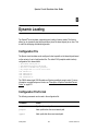
Dynamic Loading . . . . . . . . . . . . . . . . . . . . . . . . . . . . . . . . . . . . . . . . . . . . . . . . 312
Configuration File . . . . . . . . . . . . . . . . . . . . . . . . . . . . . . . . . . . . . . . . . . . . . . . . . . . . . .
Configuration File Format . . . . . . . . . . . . . . . . . . . . . . . . . . . . . . . . . . . . . . . . . . . . . . .
Precedence for the CMI Configuration File . . . . . . . . . . . . . . . . . . . . . . . . . . . . . . . . . .
Configuration File Example . . . . . . . . . . . . . . . . . . . . . . . . . . . . . . . . . . . . . . . . . . . . . .
CMI Versioning . . . . . . . . . . . . . . . . . . . . . . . . . . . . . . . . . . . . . . . . . . . . . . . . . . . . . . . .
312
312
314
315
316
Index. . . . . . . . . . . . . . . . . . . . . . . . . . . . . . . . . . . . . . . . . . . . . . . . . . . . . . . . . . . . . . . 317
January 2004
12
Product Version 5.0
Spectre Circuit Simulator User Guide
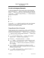
Preface
This manual assumes that you are familiar with the development, design, and simulation of
integrated circuits and that you have some familiarity with SPICE simulation. It contains
information about the Spectre® circuit simulator.
Spectre is an advanced circuit simulator that simulates analog and digital circuits at the
differential equation level. The simulator uses improved algorithms that offer increased
simulation speed and greatly improved convergence characteristics over SPICE. Besides the
basic capabilities, the Spectre circuit simulator provides significant additional capabilities over
SPICE. SpectreHDL (Spectre High-Level Description Language) and Verilog®-A use
functional description text files (modules) to model the behavior of electrical circuits and other
systems. SpectreRF adds several new analyses that support the efficient calculation of the
operating point, transfer function, noise, and distortion of common RF and communication
circuits, such as mixers, oscillators, sample holds, and switched-capacitor filters.
This Preface discusses the following topics:
■
Related Documents on page 13
■
Typographic and Syntax Conventions on page 14
■
References on page 15
Related Documents
The following can give you more information about the Spectre circuit simulator and related
products:
■
The Spectre circuit simulator is often run within the analog circuit design environment,
under the Cadence design framework II. To see how the Spectre circuit simulator is run
under the analog circuit design environment, read the Cadence Analog Design
Environment User Guide.
■
To learn more about specific parameters of components and analyses, consult the
Spectre online help (spectre -h) or the Spectre Circuit Simulator Reference
manual.
■
To learn more about the equations used in the Spectre circuit simulator, consult the
Spectre Circuit Simulator Device Model Equations manual.
January 2004
13
Product Version 5.0
Spectre Circuit Simulator User Guide
Preface
■
The Spectre circuit simulator also includes a waveform display tool, Analog Waveform
Display (AWD), to use to display simulation results. For more information about AWD,
see the Analog Waveform User Guide.
■
For more information about using the Spectre circuit simulator with SpectreHDL, see the
SpectreHDL Reference manual.
■
For more information about using the Spectre circuit simulator with Verilog-A, see the
Verilog-A Language Reference manual.
■
If you want to see how SpectreRF is run under the analog circuit design environment,
read SpectreRF Help.
■
For more information about RF theory, see SpectreRF Theory.
■
For more information about how you work with the design framework II interface, see
Cadence Design Framework II Help.
■
For more information about specific applications of Spectre analyses, see The
Designer’s Guide to SPICE & Spectre1.
Typographic and Syntax Conventions
This list describes the syntax conventions used for the Spectre circuit simulator.
literal
Nonitalic words indicate keywords that you must enter literally.
These keywords represent command (function, routine) or
option names, filenames and paths, and any other sort of type-in
commands.
argument
Words in italics indicate user-defined arguments for which you
must substitute a name or a value. (The characters before the
underscore (_) in the word indicate the data types that this
argument can take. Names are case sensitive.
|
Vertical bars (OR-bars) separate possible choices for a single
argument. They take precedence over any other character.
[ ]
Brackets denote optional arguments. When used with OR-bars,
they enclose a list of choices. You can choose one argument
from the list.
1.
Kundert, Kenneth S. The Designer’s Guide to SPICE & Spectre. Boston: Kluwer Academic Publishers, 1995.
January 2004
14
Product Version 5.0
Spectre Circuit Simulator User Guide
Preface
{ }
Braces are used with OR-bars and enclose a list of choices. You
must choose one argument from the list.
...
Three dots (...) indicate that you can repeat the previous
argument. If you use them with brackets, you can specify zero or
more arguments. If they are used without brackets, you must
specify at least one argument, but you can specify more.
Important
The language requires many characters not included in the preceding list. You must
enter required characters exactly as shown.
References
Text within brackets ([ ]) is a reference. See Appendix A, “References,” of the Spectre
Circuit Simulator Reference manual for more detailed information.
January 2004
15
Product Version 5.0
Spectre Circuit Simulator User Guide
1
Introducing the Spectre Circuit Simulator
This chapter discusses the following:
■
Improvements over SPICE on page 17
■
Analog HDLs on page 21
■
RF Capabilities on page 21
■
Mixed-Signal Simulation on page 23
■
Environments on page 23
The Spectre® circuit simulator is a modern circuit simulator that uses direct methods to
simulate analog and digital circuits at the differential equation level. The basic capabilities of
the Spectre circuit simulator are similar in function and application to SPICE, but the Spectre
circuit simulator is not descended from SPICE. The Spectre and SPICE simulators use the
same basic algorithms—such as implicit integration methods, Newton-Raphson, and direct
matrix solution—but every algorithm is newly implemented. Spectre algorithms, the best
currently available, give you an improved simulator that is faster, more accurate, more
reliable, and more flexible than previous SPICE-like simulators.
January 2004
16
Product Version 5.0
Spectre Circuit Simulator User Guide
Introducing the Spectre Circuit Simulator
Improvements over SPICE
The Spectre circuit simulator has many improvements over SPICE.
Improved Capacity
The Spectre circuit simulator can simulate larger circuits than other simulators because its
convergence algorithms are effective with large circuits, because it is fast, and because it is
frugal with memory and uses dynamic memory allocation. For large circuits, the Spectre
circuit simulator typically uses less than half as much memory as SPICE.
Improved Accuracy
Improved component models and core simulator algorithms make the Spectre circuit
simulator more accurate than other simulators. These features improve Spectre accuracy:
■
■
Advanced metal oxide semiconductor (MOS) and bipolar models
❑
The Spectre BSIM3v3 is a physics-based metal-oxide semiconductor field effect
transistor (MOSFET) model for simulating analog circuits.
❑
The Spectre models include the MOS0 model, which is even simpler and faster than
MOS1 for simulating noncritical MOS transistors in logic circuits and behavioral
models, MOS 9, EKV, BTA-HVMOS, BTA-SOI, VBIC95, TOM2, HBT, and many
more.
Charge-conserving models
The capacitance-based nonlinear MOS capacitor models used in many SPICE
derivatives can create or destroy small amounts of charge on every time step. The
Spectre circuit simulator avoids this problem because all Spectre models are chargeconserving.
■
Improved Fourier analyzer
The Spectre circuit simulator includes a two-channel Fourier analyzer that is similar in
application to the SPICE .FOURIER statement but is more accurate. The Spectre
simulator’s Fourier analyzer has greater resolution for measuring small distortion
products on a large sinusoidal signal. Resolution is normally greater than 120 dB.
Furthermore, the Spectre simulator’s Fourier analyzer is not subject to aliasing, a
common error in Fourier analysis. As a result, the Spectre simulator can accurately
compute the Fourier coefficients of highly discontinuous waveforms.
■
Better control of numerical error
January 2004
17
Product Version 5.0
Spectre Circuit Simulator User Guide
Introducing the Spectre Circuit Simulator
Many algorithms in the Spectre circuit simulator are superior to their SPICE counterparts
in avoiding known sources of numerical error. The Spectre circuit simulator improves the
control of local truncation error in the transient analysis by controlling error in the voltage
rather than the charge.
In addition, the Spectre circuit simulator directly checks Kirchhoff’s Current Law (also
known as Kirchhoff’s Flow Law) at each time step, improves the charge-conservation
accuracy of the Spectre circuit simulator, and eliminates the possibility of false
convergence.
■
Superior time-step control algorithm
The Spectre circuit simulator provides an adaptive time-step control algorithm that
reliably follows rapid changes in the solution waveforms. It does so without limiting
assumptions about the type of circuit or the magnitude of the signals.
■
More accurate simulation techniques
Techniques that reduce reliability or accuracy, such as device bypass, simplified models,
or relaxation methods, are not used in the Spectre circuit simulator.
■
User control of accuracy tolerances
For some simulations, you might want to sacrifice some degree of accuracy to improve
the simulation speed. For other simulations, you might accept a slower simulation to
achieve greater accuracy. With the Spectre circuit simulator, you can make such
adjustments easily by setting a single parameter.
Improved Speed
The Spectre circuit simulator is designed to improve simulation speed. The Spectre circuit
simulator improves speed by increasing the efficiency of the simulator rather than by
sacrificing accuracy.
■
Faster simulation of small circuits
The average Spectre simulation time for small circuits is typically two to three times faster
than SPICE. The Spectre circuit simulator can be over 10 times faster than SPICE when
SPICE is hampered by discontinuity in the models or problems in the code. Occasionally,
the Spectre circuit simulator is slower when it finds ringing or oscillation that goes
unnoticed by SPICE. This can be improved by setting the macromodels option to yes.
■
Faster simulation for large circuits
January 2004
18
Product Version 5.0
Spectre Circuit Simulator User Guide
Introducing the Spectre Circuit Simulator
The Spectre circuit simulator is generally two to five times faster than SPICE with large
circuits because it has fewer convergence difficulties and because it rapidly factors and
solves large sparse matrices.
Improved Reliability
The Spectre circuit simulator offers you the following improvements in reliability:
■
Improved convergence
Spectre proprietary algorithms ensure convergence of the Newton-Raphson algorithm in
the DC analysis. The Spectre circuit simulator virtually eliminates the convergence
problems that earlier simulators had with transient simulation.
■
Helpful error and warning messages
The Spectre circuit simulator detects and notifies you of many conditions that are likely
to be errors. For example, the Spectre circuit simulator warns of models used in
forbidden operating regions, of incorrectly wired circuits, and of erroneous component
parameter values. By identifying such common errors, the Spectre circuit simulator
saves you the time required to find these errors with other simulators.
The Spectre circuit simulator lets you define soft parameter limits and sends you
warnings if parameters exceed these limits.
■
Thorough testing
Automated tests, which include over 1,000 test circuits, are constantly run on all
hardware platforms to ensure that the Spectre circuit simulator is consistently reliable
and accurate.
■
Benchmark suite
There is an independent collection of SPICE netlists that are difficult to simulate. You can
obtain these circuits from the Microelectronics Center of North Carolina (MCNC) if you
have File Transfer Protocol (FTP) access on the Internet. You can also get information
about the performance of several simulators with these circuits.
The Spectre circuit simulator has successfully simulated all of these circuits. Sometimes
the netlists required minor syntax corrections, such as inserting balancing parentheses,
but circuits were never altered, and options were never changed to affect convergence.
January 2004
19
Product Version 5.0
Spectre Circuit Simulator User Guide
Introducing the Spectre Circuit Simulator
Improved Models
The Spectre circuit simulator has MOSFET Level 0–3, BSIM1, BSIM2, BSIM3, BSIM3v3,
EKV, MOS9, JFET, TOM2, GaAs MESFET, BJT, VBIC, HBT, diode, and many other models.
It also includes the temperature effects, noise, and MOSFET intrinsic capacitance models.
The Spectre Compiled Model Interface (CMI) option lets you integrate new devices into the
Spectre simulator using a very powerful, efficient, and flexible C language interface. This CMI
option, the same one used by Spectre developers, lets you install proprietary models.
Spectre Usability Features and Customer Service
The following features and services help you use the Spectre circuit simulator easily and
efficiently:
■
You can use Spectre soft limits to catch errors created by typing mistakes.
■
Spectre diagnosis mode, available as an options statement parameter, gives you
information to help diagnose convergence problems.
■
You can run the Spectre circuit simulator standalone or run it under the Cadence® analog
design environment. To see how the Spectre circuit simulator is run under the analog
circuit design environment, read the Cadence Analog Design Environment User
Guide. You can also run the Spectre circuit simulator in the Composer-to-Spectre direct
simulation environment. The environment provides a graphical user interface for running
the simulation.
■
The Spectre circuit simulator gives you an online help system. With this system, you can
find information about any parameter associated with any Spectre component or
analysis. You can also find articles on other topics that are important to using the Spectre
circuit simulator effectively.
■
The Spectre circuit simulator also includes a waveform display tool, Analog Waveform
Display (AWD), to use to display simulation results. For more information about AWD,
see the Analog Waveform User Guide.
■
If you experience a stubborn convergence or accuracy problem, you can send the circuit
to Customer Support to get help with the simulation. For current phone numbers and email addresses, see the following web site:
http://sourcelink.cadence.com/supportcontacts.html
January 2004
20
Product Version 5.0
Spectre Circuit Simulator User Guide
Introducing the Spectre Circuit Simulator
Analog HDLs
The Spectre circuit simulator works with two analog high-level description languages
(AHDLs): SpectreHDL and Verilog®-A. These languages are part of the Spectre Verilog-A
option. SpectreHDL is proprietary to Cadence and is provided for backward compatibility. The
Verilog-A language is an open standard, which was based upon SpectreHDL. The Verilog-A
language is preferred because it is upward compatible with Verilog-AMS, a powerful and
industry-standard mixed-signal language.
Both languages use functional description text files (modules) to model the behavior of
electrical circuits and other systems. Each programming language allows you to create your
own models by simply writing down the equations. The AHDL lets you describe models in a
simple and natural manner. This is a higher level modeling language than previous modeling
languages, and you can use it without being concerned about the complexities of the
simulator or the simulator algorithms. In addition, you can combine AHDL components with
Spectre built-in primitives.
Both languages let designers of analog systems and integrated circuits create and use
modules that encapsulate high-level behavioral descriptions of systems and components.
The behavior of each module is described mathematically in terms of its terminals and
external parameters applied to the module. Designers can use these behavioral descriptions
in many disciplines (electrical, mechanical, optical, and so on).
Both languages borrow many constructs from Verilog and the C programming language.
These features are combined with a minimum number of special constructs for behavioral
simulation. These high-level constructs make it easier for designers to use a high-level
description language for the first time.
RF Capabilities
SpectreRF adds several new analyses that support the efficient calculation of the operating
point, transfer function, noise, and distortion of common analog and RF communication
circuits, such as mixers, oscillators, sample and holds, and switched-capacitor filters.
SpectreRF adds four types of analyses to the Spectre simulator. The first is periodic steadystate (PSS) analysis, a large-signal analysis that directly computes the periodic steady-state
response of a circuit. With PSS, simulation times are independent of the time constants of the
circuit, so PSS can quickly compute the steady-state response of circuits with long time
constants, such as high-Q filters and oscillators.
You can also embed a PSS analysis in a sweep loop (referred to as an SPSS analysis in the
Cadence analog design environment), which allows you to easily determine harmonic levels
January 2004
21
Product Version 5.0
Spectre Circuit Simulator User Guide
Introducing the Spectre Circuit Simulator
as a function of input level or frequency, making it easy to measure compression points,
intercept points, and voltage-controlled oscillator (VCO) linearity.
The second new type of analysis is the periodic small-signal analysis. After completing a PSS
analysis, SpectreRF can predict the small-signal transfer functions and noise of frequency
translation circuits, such as mixers or periodically driven circuits such as oscillators or
switched-capacitor or switched-current filters. The periodic small-signal analyses—periodic
AC (PAC) analysis, periodic transfer function (PXF) analysis, and periodic noise (Pnoise)
analysis—are similar to Spectre’s AC, XF, and Noise analyses, but the traditional small-signal
analyses are limited to circuits with DC operating points. The periodic small-signal analyses
can be applied to circuits with periodic operating points, such as the following:
■
Mixers
■
VCOs
■
Switched-current filters
■
Phase/frequency detectors
■
Frequency multipliers
■
Chopper-stabilized amplifiers
■
Oscillators
■
Switched-capacitor filters
■
Sample and holds
■
Frequency dividers
■
Narrow-band active circuits
The third SpectreRF addition to Spectre functionality is periodic distortion (PDISTO) analysis.
PDISTO analysis directly computes the steady-state response of a circuit driven with a large
periodic signal, such as an LO (local oscillation) or a clock, and one or more tones with
moderate level. With PDISTO, you can model periodic distortion and include harmonic
effects. PDISTO computes both a large signal, the periodic steady-state response of the
circuit, and also the distortion effects of a specified number of moderate signals, including the
distortion effects of the number of harmonics that you choose. This is a common scenario
when trying to predict the intermodulation distortion of a mixer, amplifier, or a narrow-band
filter. In this analysis, the tones can be large enough to create significant distortion, but not
so large as to cause the circuit to switch or clip. The frequencies of the tones need not be
periodically related to each other or to the large signal LO or clock. Thus, you can make the
tone frequencies very close to each other without penalty, which allows efficient computation
of intermodulation distortion of even very narrow band circuits.
January 2004
22
Product Version 5.0
Spectre Circuit Simulator User Guide
Introducing the Spectre Circuit Simulator
The fourth analysis that SpectreRF adds to the Spectre circuit simulator is the envelopefollowing analysis. This analysis computes the envelope response of a circuit. The simulator
automatically determines the clock period by looking through all the sources with the
specified name. Envelope-following analysis is most efficient for circuits where the
modulation bandwidth is orders of magnitude lower than the clock frequency. This is typically
the case, for example, in circuits where the clock is the only fast varying signal and other input
signals have a spectrum whose frequency range is orders of magnitude lower than the clock
frequency. For another example, the down conversion of two closely placed frequencies can
also generate a slow-varying modulation envelope. The analysis generates two types of
output files, a voltage versus time (td) file, and an amplitude/phase versus time (fd) file for
each specified harmonic of the clock fundamental.
In summary, with periodic small-signal analyses, you apply a small signal at a frequency that
might not be harmonically related (noncommensurate) to the periodic response of the
undriven system, the clock. This small signal is assumed to be small enough so that the circuit
is unaffected by its presence.
With PDISTO, you can apply one or two additional signals at frequencies not harmonically
related to the large signal, and these signals can be large enough to drive the circuit to
behave nonlinearly.
For complex nonlinear circuits, hand calculation of noise or transfer function is virtually
impossible. Without SpectreRF, these circuits must be breadboarded to determine their
performances. SpectreRF eliminates unnecessary breadboarding, saving time.
Mixed-Signal Simulation
You can use the Spectre circuit simulator coupled with the Verilog-XL simulator in the
Cadence analog design environment to simulate mixed analog and digital circuits efficiently.
This mixed-signal simulation solution can easily handle complex designs with tens of
thousands of transistors and tens of thousands of gates. The digital Verilog data can come
from the digital designer as either an RTL block or gates out of synthesis.
Environments
The Spectre circuit simulator is fully integrated into the Cadence design framework II for the
Cadence analog design environment and also into the Cadence analog workbench design
system. You can also use the Spectre circuit simulator by itself with several different output
format options.
Assura interactive verification, Dracula® distributed multi-CPU option, and Assura
hierarchical physical verification produce a netlist that can be read into the Spectre circuit
January 2004
23
Product Version 5.0
Spectre Circuit Simulator User Guide
Introducing the Spectre Circuit Simulator
simulator. However, only interactive verification when used with the Cadence analog design
environment automatically attaches the stimulus file. All other situations require a stimulus file
as well as device models.
January 2004
24
Product Version 5.0
Spectre Circuit Simulator User Guide
2
Getting Started with Spectre
This chapter discusses the following topics:
■
Using the Example and Displaying Results on page 26
■
Sample Schematic on page 26
■
Sample Netlist on page 28
■
Instructions for a Spectre Simulation Run on page 32
■
Viewing Your Output on page 34
January 2004
25
Product Version 5.0
Spectre Circuit Simulator User Guide
Getting Started with Spectre
Using the Example and Displaying Results
In this chapter, you examine a schematic and its Spectre® circuit simulator netlist to get an
overview of Spectre syntax. You also follow a sample circuit simulation. The best way to use
this chapter depends on your past experience with simulators.
Carefully examine the schematic (“Sample Schematic” on page 26) and netlist (“Sample
Netlist” on page 28) and compare Spectre netlist syntax with that of SPICE-like simulators
you have used. If you have prepared netlists for SPICE-like simulators before, you can skim
“Elements of a Spectre Netlist” on page 29. With this method, you can learn a fair amount
about the Spectre simulator in a short time.
Approach this chapter as an overview. You will probably have unanswered questions about
some topics when you finish the chapter. Each topic is covered in greater depth in subsequent
chapters. Do not worry about learning all the details now.
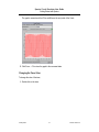
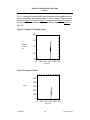
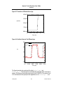
To give you a complete overview of a Spectre simulation, the example in this chapter includes
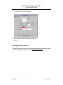
the display of simulation results with WaveScan, a waveform display tool that is included with
the Spectre simulator. If you use another display tool, the procedures you follow to display
results are different. This user guide does not teach you how to display waveforms with
different tools. If you need more information about how to display Spectre results, consult the
documentation for your display tool.
The example used in this chapter is a small circuit, an oscillator; you run a transient analysis
on the oscillator and then view the results. The following sections contain the schematic and
netlist for the oscillator. If you have used SPICE-like simulators before, looking at the
schematic and netlist can help you compare Spectre syntax with those of other simulators. If
you are new to simulation, looking at the schematic and netlist can prepare you to understand
the later chapters of this book.
You can also get more information about command options, components, analyses, controls,
and other selected topics by using the spectre -h command to access the Spectre online
help.
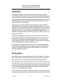
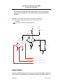
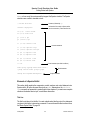
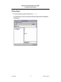
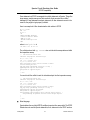
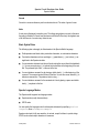
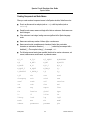
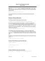
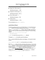
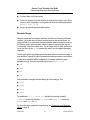
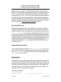
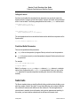
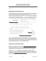
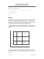
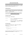
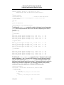
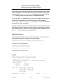
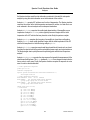
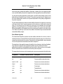
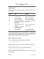
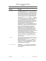
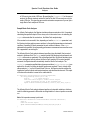
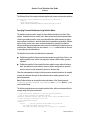
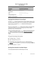
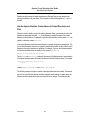
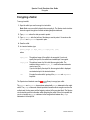
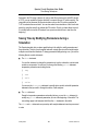
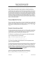
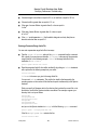
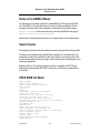
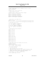
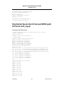
Sample Schematic
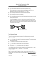
A schematic is a drawing of an electronic circuit, showing the components graphically and
how they are connected together. The following schematic has several annotations:
■
Names of components
Each component is labeled with the name that appears in the instance statement for that
component. The names for components are in italics (for example, Q2).
January 2004
26
Product Version 5.0
Spectre Circuit Simulator User Guide
Getting Started with Spectre
■
Names of nodes
Each node in the circuit is labeled with its unique name or number. This name can be
either a name you create or a number. Names of nodes are in boldface type (for example,
b1). Ground is node 0.
■
Sample instance statements
January 2004
27
Product Version 5.0
Spectre Circuit Simulator User Guide
Getting Started with Spectre
The schematic is annotated with instance statements for some of the components.
Arrows connect the components in the schematic with their corresponding instance
statements.
Bold Type = Names of nodes. All connections to ground have the same node name.
Italic Type = Names of components (also appear in the instance statement for each
component).
= Link between components and instance statements.
∼
∼
Vcc
Vcc
cc
cc
C1
L1
out
•
∼cc
Vcc
C2
b1
b2
•
Q1
•
e
Q2
•
R1
Iee
C3
C4
R2
Q1 (cc b1 e) npn
C3 (b1 0) capacitor c=3nF
R1 (b1 0) resistor r=10k
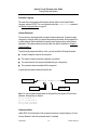
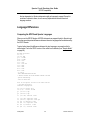
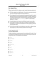
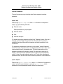
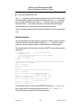
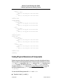
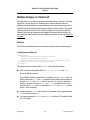
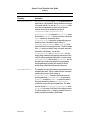
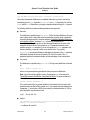
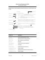
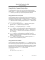
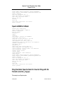
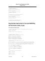
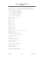
Sample Netlist
A netlist is an ASCII file that lists the components in a circuit, the nodes that the components
are connected to, and parameter values. You create the netlist in a text editor such as vi or
January 2004
28
Product Version 5.0
Spectre Circuit Simulator User Guide
Getting Started with Spectre
emacs or from one of the environments that support the Spectre simulator. The Spectre
simulator uses a netlist to simulate a circuit.
// BJT ECP Oscillator
Comment (indicated by //)
simulator lang=spectre
Indicates the file contains a Spectre netlist
(see the next section). Place below first line.
Iee (e 0)
isource dc=1mA
Vcc (cc 0) vsource dc=5
Q1
Q2
(cc b1 e) npn
(out b2 e) npn
L1
(cc out) inductor l=1uH
C1
C2
C3
C4
(cc out) capacitor c=1pf
(out b1) capacitor c=272.7pF
(b1 0) capacitor c=3nF
(b2 0) capacitor c=3nF
R1
R2
(b1
(b2
Instance statements
0) resistor r=10k
0) resistor r=10k
Control statement (sets initial conditions)
ic cc=5
model npn bjt type=npn bf=80 rb=100 vaf=50 \
cjs=2pf tf=0.3ns tr=6ns cje=3pf cjc=2pf
Model statement
Analysis statement
OscResp tran stop=80us maxstep=10ns
Elements of a Spectre Netlist
This section briefly explains the components, models, analyses, and control statements in a
Spectre netlist. All topics discussed here (such as model statements or the simulator
lang command) are presented in greater depth in later chapters. If you want more complete
reference information about a topic, consult these discussions.
Title Line
The first line is taken to be the title. It is used verbatim when labeling output. Any statement
you place in the first line is ignored as a comment. For more information about comment lines,
see “Basic Syntax Rules” on page 59.
January 2004
29
Product Version 5.0
Spectre Circuit Simulator User Guide
Getting Started with Spectre
Simulation Language
The second line of the sample netlist indicates that the netlist is in the Spectre Netlist
Language, instead of SPICE. For more information about the simulator lang command,
see Spectre Language Modes on page 59.
Instance Statements
The next section in the sample netlist consists of instance statements. To specify a single
component in a Spectre netlist, you place all the necessary information for the component in
a netlist statement. Netlist statements that specify single components are called instance
statements. (The instance statement also has other uses that are described in Chapter 4,
“Spectre Netlists.”)
To specify single components within a circuit, you must provide the following information:
■
A unique component name for the component
■
The names of nodes to which the component is connected
■
The master name of the component (identifies the type of component)
■
The parameter values associated with the component
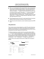
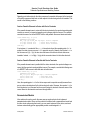
A typical Spectre instance statement looks like this:
Component name
R16 (4 0) resistor r=100
Node names
Parameter value
Master name
Note: You can use balanced parentheses to distinguish the various parts of the instance
statement, although they are optional:
R1
Q1
Gm
R7
(1
(c
(1
(x
2) resistor r=1
b e s) npn area=10
2)(3 4) vccs gm=.01
y) rmod (r=1k w=2u)
Component Names
Unlike SPICE, the first character of the component name has no special meaning. You can
use any character to start the component name. For example:
January 2004
30
Product Version 5.0
Spectre Circuit Simulator User Guide
Getting Started with Spectre
Load (out o) resistor r=50
Balun (in o pout nout) transformer
Note: You can find the exact format for any component in the parameter listings for that
component in the Spectre online help.
Master Names
The type of a component depends on the name of the master, not on the first letter of the
component name (as in SPICE); this feature gives you more flexibility in naming components.
The master can be a built-in primitive, a model, a subcircuit, or an AHDL component.
Parameter Values
Real numbers can be specified using scientific notation or common engineering scale factors.
For example, you can specify a 1 pF capacitor value either as c=1pf or c=1e-12. Depending
on whether you are using the Spectre Netlist Language or SPICE, you might need to use
different scale factors for parameter values. Only ANSI standard scale factors are used in
Spectre netlists. For more information about scale factors, see Instance Statements on
page 62.
Control Statements
The next section of the sample netlist contains a control statement, which sets initial
conditions.
Model Statements
Some components allow you to specify parameters common to many instances using the
model statement. The only parameters you need to specify in the instance statement are
those that are generally unique for a given instance of a component.
You need to provide the following for a model statement:
■
The keyword model at the beginning of the statement
■
A unique name for the model (reference by master names in instance statements)
■
The master name of the model (identifies the type of model)
■
The parameter values associated with the model
January 2004
31
Product Version 5.0
Spectre Circuit Simulator User Guide
Getting Started with Spectre
The following example is a model statement for a bjt. The model name is npn¸ and the
component type name is bjt. The backslash (\) tells you that the statement continues on the
next line. The backslash must be the last character in the line because it escapes the carriage
return.
model npn bjt type=npn bf=80 rb=100 vaf=50 \
cjs=2pf tf=0.3ns tr=6ns cje=3pf cjc=2pf
When you create an instance statement that refers to a model statement for its parameter
values, you must specify the model name as the master name. For example, an instance
statement that receives its parameter values from the previous model statement might look
like this:
Q1
(vcc b1 e vcc) npn
Check documentation for components to determine which parameters are expected to be
provided on the instance statement and which are expected on the model statement.
Analysis Statements
The last section of the sample netlist has the analysis statement. An analysis statement has
the same syntax as an instance statement, except that the analysis type name replaces the
master name. To specify an analysis, you must include the following information in a netlist
statement:
■
A unique name for the analysis statement
■
Possibly a set of node names
■
The name of the type of analysis you want
■
Any additional parameter values associated with the analysis
To find the analysis type name and the parameters you can specify for an analysis, consult
the parameter listing for that analysis in the Spectre online help (spectre -h).
The following analysis statement specifies a transient analysis. The analysis name is
stepResponse, and the analysis type name is tran.
stepResponse tran stop=100ns
Instructions for a Spectre Simulation Run
When you complete a netlist, you can run the simulation with the spectre command.
➤
To run a simulation for the sample circuit, type the following at the command line:
spectre osc.scs
January 2004
32
Product Version 5.0
Spectre Circuit Simulator User Guide
Getting Started with Spectre
Note: osc.scs is the file that contains the netlist.
Following Simulation Progress
As the simulation runs, the Spectre simulator sends messages to your screen that show the
progress of the simulation and provide statistical information. In the simulation of osc.scs,
the Spectre simulator prints some warnings and notifications. The Spectre simulator tells you
about conditions that might reduce simulation accuracy. When you see a Spectre warning or
notification, you must decide whether the information is significant for your particular
simulation.
Screen Printout
The printout for the osc.scs simulation looks like this:
spectre (ver. 5.0.0.052603 -- 27 May 2003).
Simulating `osc.scs' on cds11047 at 1:21:54 PM, Wed Aug 20, 2003.
Circuit inventory:
nodes
equations
bjt
capacitor
inductor
isource
resistor
vsource
5
9
2
4
1
1
2
1
***************************************************
Transient Analysis `OscResp': time = (0 s -> 80 us)
***************************************************
Narration of transient
analysis progress
.....9.....8......7......6......5......4......3......2.....1......0
Number of accepted tran steps = 23508.
Initial condition solution time = 0 s.
Intrinsic tran analysis time = 7.07 s.
Total time required for tran analysis `OscResp' was 7.08 s.
Aggregate audit (1:22:02 PM, Wed Aug 20, 2003):
Time used: CPU = 7.29 s, elapsed = 8 s, util. = 91.1%.
Virtual memory used = 1.3 Mbytes.
spectre completes with 0 errors, 0 warnings, and 0 notices
January 2004
33
Product Version 5.0
Spectre Circuit Simulator User Guide
Getting Started with Spectre
Viewing Your Output
The waveform display tool for this simulation example is WaveScan, a display tool you receive
when you purchase the Spectre simulator. In this section you will learn the following:
■
How to start WaveScan
■
How to plot signals
■
How to change the color of a trace
Starting WaveScan
➤
Type the following at the command line:
wavescan &
Note: To start WaveScan for the simulation example, type the following at the command
line (from the directory where the Spectre simulator was run):
wavescan -dataDir osc.raw
The Results Browser window appears with the osc.raw data directory displayed in the
right panel.
January 2004
34
Product Version 5.0
Spectre Circuit Simulator User Guide
Getting Started with Spectre
Plotting Signals
1. In the Results Browser window, double-click on osc.raw.
The data directory moves to the left panel and the associated signals are displayed in
the right panel.
January 2004
35
Product Version 5.0
Spectre Circuit Simulator User Guide
Getting Started with Spectre
2. Right-click on the signal you want to plot (for example, out) and choose New Win from
the pop-up menu. The Graph Display window appears.
3. Choose Zoom – X-Zoom.
The
cursor is displayed on the Graph Display window.
4. Left-click at around 70us and, drag, and release the mouse button at around 80us.
January 2004
36
Product Version 5.0
Spectre Circuit Simulator User Guide
Getting Started with Spectre
The graph is zoomed such that 70us and 80us are the end points of the X-axis.
5. Click Zoom – Fit to return the graph to the unzoomed state.
Changing the Trace Color
To change the color of the trace,
1. Double-click on the trace.
January 2004
37
Product Version 5.0
Spectre Circuit Simulator User Guide
Getting Started with Spectre
The Trace Attributes dialog box appears.
2. In the Foreground field, select the color for the trace.
3. Click OK.
Learning More about WaveScan
The WaveScan display tool gives you a number of additional options for displaying your data.
To learn more about using WaveScan, see the WaveScan User Guide.
January 2004
38
Product Version 5.0
Spectre Circuit Simulator User Guide
Getting Started with Spectre
January 2004
39
Product Version 5.0
Spectre Circuit Simulator User Guide
Getting Started with Spectre
January 2004
40
Product Version 5.0
Spectre Circuit Simulator User Guide
3
SPICE Compatibility
While SPICE is an industry-standard language, there are many variations of SPICE syntax
on the market today. Most of the language is common across the major commercial
simulators, but each vendor has extended or modified it with different capabilities and/or
slightly different syntax. For the convenience of SPICE users, the Spectre® circuit simulator
provides a SPICE Reader as an extension to its native language that accepts most variations
of SPICE input. The SPICE Reader provides support for SPICE2, SPICE3, and common
extensions found in other simulators such as PSPICE and HSPICE. This chapter focuses on
how to use the SPICE Reader with Spectre. This chapter is not intended to describe the
syntax variations of SPICE, as they are well documented in other places, nor an exact listing
of syntax supported by the SPICE Reader.
■
Reading SPICE Netlists on page 42
■
Language Differences on page 48
■
Scope of the Compatibility on page 51
January 2004
41
Product Version 5.0
Spectre Circuit Simulator User Guide
SPICE Compatibility
Reading SPICE Netlists
Spectre provides the SPICE Reader to let you simulate existing SPICE netlists with Spectre.
While it is possible to gain access to many of Spectre’s features with a SPICE netlist, the
Spectre syntax is a much more powerful language designed to give the Spectre user features
beyond those provided by SPICE. Whenever possible, you are encouraged to take advantage
of Spectre’s native language. When Spectre syntax is not an acceptable solution, the SPICE
Reader can be used to ensure access to as much of Spectre’s capabilities as possible.
Running the SPICE Reader
In order for Spectre to properly process a SPICE netlist, the SPICE Reader must be enabled.
By default the SPICE Reader is disabled when you invoke Spectre. Use the command
spectrespp rather than the spectre command to enable the SPICE Reader. For example,
the following command invokes Spectre with the SPICE Reader for the input netlist amp.sp:
spectrespp amp.sp
The Spice Reader runs on the top-level netlist, as well as on any included files that contain
SPICE syntax. The SPICE Reader converts the netlist to Spectre native syntax before it
sends the design to the Spectre netlist reader. From the 5.0 release, any .measure
statements found in the Spice input file are converted to MDL (Measurement Description
Language) before being passed on to Spectre. The conversion is done via the creation of an
MDL control file, which is written to the current directory. This control file takes on the name
of the netlist, with a suffix of .mdl. The simulation that immediately follows the conversion
uses the MDL option to Spectre with this control file to evaluate the .measure expressions.
Results are written to a file with the same name as the control file (netlist) with a .measure
suffix. For example, the amp.sp SPICE netlist above creates a control file named amp.mdl,
and a measurement output file named amp.measure. You simply enter the spectrespp
command with the netlist, and the rest of the steps are completed for you automatically. The
MDL control file is left behind for future use.
Note: In previous releases, the command line option +spp was used to invoke the SPICE
Reader. While this method is still supported, it is advised that you use the spectrespp
command if .measure statements are included in the input file. For more information on
MDL, see the SpectreMDL User Guide and Reference.
For backward compatibility, a limited SPICE2 netlist reader is embedded into the Spectre
netlist reader. This reader supports much of SPICE2G6 syntax and has as its primary use the
processing of SPICE-style model cards. If the SPICE Reader is not used, this limited SPICE
netlist reader is used. This is only for backwards compatibility and might be removed in a
future release, to be replaced by the SPICE Reader. This limited SPICE netlist reader is no
longer documented as of the 4.4.3 release. In the rest of this chapter, “SPICE Reader” refers
to the full SPP SPICE Reader, and not this limited version.
January 2004
42
Product Version 5.0
Spectre Circuit Simulator User Guide
SPICE Compatibility
Running the SPICE Reader from Cadence Analog Design Environment
When using Spectre within Cadence Analog Design Environment, the need to read SPICE
netlists is usually limited to model files and information from extraction tools that comes into
the netlist by included files. For all other design data, Analog Artist produces netlists in the
Spectre native syntax. You can enable the use of the SPICE Reader by choosing the Setup
-> Environment form and toggling the Use SPICE Netlist Reader (spp) button to Y. Be sure
that you do not have any relative paths specified for included files, such as model files, and
that the Include Path field in the Setup -> Simulation Files field is blank. The SPICE
Reader’s inability to handle relative paths is documented in the Spectre Known
Problems and Solutions.
Running the SPICE Reader from the Command Line
When you run Spectre from the command line (outside of the Artist/Composer environment),
the SPICE Reader is disabled by default. As described in “Running the SPICE Reader” on
page 42, you must use the spectrespp command for the SPICE Reader to process the toplevel netlist:
spectrespp opamp.sp
This command calls Spectre with the spp and mdl command line options. There are several
command line options that can be used in conjunction with spectrespp:
Specifying the Design File
The command line option -design is used to identify the input file. In the absence of any
command line options, the single argument after the spectrespp command is assumed to
be the input netlist. Therefore the following commands are identical:
spectrespp opamp.sp
spectrespp -design opamp.sp
Specifying the spp Binary to be Used
By default, the spp binary that is located in the Cadence hierarchy,
your_install_directory/tools/dfII/bin/spp,is used by the spectrespp
command. You can specify the use of other spp executables with the -sppbin command line
option. In the following example, spp from the current directory is used:
spectrespp -sppbin ./spp opamp.sp
January 2004
43
Product Version 5.0
Spectre Circuit Simulator User Guide
SPICE Compatibility
Specifying the Location of the Measurement Output
The command line option -measure is used to specify the location of the measurement output.
The following command
spectrespp -measure design.measure -design opamp.sp
writes the output to design.measure. If you do not use this option, the output of the
.measure statement is written to a file with the same base name as the netlist and the suffix
.measure. In the above example, this would be opamp.measure.
Notice that when specifying the -measure option, you must also specify the -design option
to identify the netlist.
All other command line options are passed to Spectre. Type spectrespp -usage for online
help.
Using the SPICE Reader to Convert Netlists
In many cases, the SPICE data to be used with Spectre is a library of models or reusable
blocks (that is, subcircuits). Rather than using the SPICE Reader to interpret these files each
time they are used, you can convert the netlist to Spectre’s native syntax. This is done by
running the SPICE Reader alone (spp) and using the -convert option. The -convert
option removes special embedded codes for tracking the line numbers of the original netlist,
returning a cleanly converted netlist.
spp -convert -iofile inputFile [outputFile]
or
spp -convert < inputFile [ > [outputFile] ]
where
spp
Runs the SPICE reader.
-convert
Converts the SPICE netlist to an equivalent Spectre netlist. This
option does not descend into included files to convert them but
only converts the include statement. Included files must be
converted independently. In this case, the SPICE Reader
cannot always resolve conflicts and ambiguities, and you must
verify the resulting netlist files.
January 2004
44
Product Version 5.0
Spectre Circuit Simulator User Guide
SPICE Compatibility
-iofile
Replaces all instances of the input file name (in include
statements) with the output file name in the converted netlist.
Do not put < > around the input file name if you use this
option.
inputFile
The SPICE netlist to be converted. Put < > around the input file
name only if you do not use the iofile option.
outputFil
The file name for the converted netlist. If you do not specify this,
the converted netlist is displayed at standard output — i.e., in
the terminal window.
Examples
The following command converts the SPICE netlist amp.sp to an equivalent Spectre netlist
and displays the result in the terminal window:
spp -convert < amp.sp
The following command converts the SPICE netlist amp.sp to an equivalent Spectre netlist
with the name amp.scs:
spp -convert < amp.sp > amp.scs
The following command converts the SPICE netlist amp.sp to an equivalent Spectre netlist
with the name test.scs. All references to amp.sp in the input file are replaced by
test.scs in the output file.
spp -convert -iofile amp.sp test.scs
Converting Hierarchically Arranged Netlists
Great care must be taken when converting hierarchically arranged netlists. Some of the
possible issues include the following:
■
Distinguishing instance models from instance parameters
For some devices, such as resistors, SPICE instance statements can use an orderdependent mechanism to define the values of parameters. An example could be
r1 1 0 myres
The field myres could be either a model name or a parameter representing the
resistance value in SPICE. The SPICE Reader maps this to a parameter if a .param
statement is encountered with this assignment or to a model name if a model card with
the name myres is found. If neither is present, the field is assumed to be a model name.
In the case of the -convert mode, where these assignments could be part of included
January 2004
45
Product Version 5.0
Spectre Circuit Simulator User Guide
SPICE Compatibility
files, this assumption could be incorrect, and the instance statement would need to be
fixed.
■
Global nodes
In Spectre, global nodes must be at the very beginning of the netlist, while they can be
present anywhere in a SPICE netlist. If a converted file contains global nodes, these
must be moved to the top level of the netlist before the file can be included in a higher
level netlist. Multiple global statements cause fatal errors in Spectre.
■
Location of measurement data
The SPICE Reader converts Hspice style .measure statements to Measurement
Description Language (MDL) statements. The SPICE Reader does this by creating an
MDL control file, which can then be used in the simulation. In normal operation (using
the spectrespp <netlist> command), the control file that is created takes on the
name of the netlist, with the suffix .mdl. When a netlist is converted with the -convert
option, the MDL control file that is created is always named Netlist.mdl. If this control
file is used in a subsequent simulation, the results output is written to a file named
Netlist.measure. For example, say that you have an SPICE netlist named amp.sp.
In order to convert this netlist without executing the simulation, use spp with the
-convert option:
spp -convert < amp.sp > amp.scs
Upon completion of this command, the Spectre equivalent for amp.sp is in the amp.scs
file. In addition, a file called Netlist.mdl is created. This additional file contains the
MDL expressions that correspond to any .measure statements in the original netlist. In
order to run the Spectre simulation using the new netlist and control file, use the following
command:
spectremdl -batch Netlist.mdl -design amp.scs
Upon completion of the simulation, you’ll find a file named Netlist.measure, which
contains the values calculated for each of the MDL expressions.
For more information on the expression evaluation capabilities in Spectre, see the
SpectreMDL User Guide and Reference.
■
Netlist parameters
In Spectre, parameters are order dependent; that is, they must be defined before being
used. When the SPICE Reader is run on the entire design, parameters are moved to the
top of the netlist, but, in convert mode, they are moved to the top of each file. If a
parameter is accessed before inclusion, it will fail until it is fixed.
■
Order-dependent statements
January 2004
46
Product Version 5.0
Spectre Circuit Simulator User Guide
SPICE Compatibility
Some statements in SPICE are mapped into multiple statements in Spectre. Things like
temp sweeps, analysis sweeps, and alter sections all get converted into multiline
statements. If temp statements, analysis statements, or alter statements are not in the
same file, they might not get properly unfolded.
Here is an example of a Mos characterization deck written in SPICE:
M1 1 2 0 0 NCH
VDR 1 0 2
VG 2 0 1
.OP
.MODEL NCH NMOS LEVEL=49
+ TOX=1e-9 VTH0=0.5 VBOX=5
.TEMP 25 75 100
.INCLUDE "dcAnalysis.inc"
.END
where dcAnalysis.inc is
.DC VDR 0 5 0.1 VG 0 2 0.1
The netlist produced with spp -convert does not include the sweep statement within
the temperature sweep:
//
Mos characterization deck
simulator lang=spectre insensitive=yes
m1 ( 1 2 0 0 ) nch
vdr ( 1 0 ) vsource dc=2
vg ( 2 0 ) vsource dc=1
model nch bsim3v3 type=n tox=1e-9 vth0=0.5 vbox=5
include "dcAnalysis.inc"
swp_tmp1 sweep param=temp values=[25 75 100] {
sppSaveOptions options save=allpub
analysisOP1 dc oppoint=logfile
}
// end
You need to edit the netlist to insert the included analysis into the temperature sweep:
//
Mos characterization deck
simulator lang=spectre insensitive=yes
m1 ( 1 2 0 0 ) nch
vdr ( 1 0 ) vsource dc=2
vg ( 2 0 ) vsource dc=1
model nch bsim3v3 type=n tox=1e-9 vth0=0.5 vbox=5
swp_tmp1 sweep param=temp values=[25 75 100] {
sppSaveOptions options save=allpub
analysisOP1 dc oppoint=logfile
analysisDCswp1 sweep param=dc dev=vg start=0 stop=2 step=0.1 {
analysisDCswp2 dc param=dc dev=vdr start=0 stop=5 step=0.1
}
}
// end
■
Mixed language
Spectre allows the use of both SPICE and Spectre syntax in the same netlist. The SPICE
Reader does not read the Spectre statements; thus, statements in the SPICE sections
January 2004
47
Product Version 5.0
Spectre Circuit Simulator User Guide
SPICE Compatibility
that are dependent on Spectre statements might get improperly mapped. Except for
model and subcircuit names, do not have any dependencies between these two
language sections.
Language Differences
Comparing the SPICE and Spectre Languages
When you run the SPICE Reader, all SPICE statements are mapped directly to Spectre input.
There are several important differences between these two languages that are addressed by
the SPICE Reader.
To get a better idea at the differences between the two languages, an example netlist is
shown below. First is the SPICE version of the netlist for an oscillator (from “Sample Netlist”
on page 28):
BJT ECP Oscillator
Vcc 1 0 5
Iee 2 0 1MA
Q1 1 3 2 NPN
Q2 4 5 2 NPN
L1 4 5 1UH
C1 1 5 1PF
C2 5 3 272.7PF
C3 3 0 3NF
C4 5 6 3NF
R1 3 0 10K
R2 5 6 10K
.ic V(3)=1
.model NPN NPN BF=80 RB=100
+ VAF=50 CJS=2PF TF=0.3NS TR=6NS CJE=3PF CJC=2PF
.option method=trap
.tran 1us 80us 10ns
Here is the Spectre version of the same netlist:
// BJT ECP Oscillator
simulator lang=spectre
Vcc (vcc 0) vsource dc=5
Iee (e 0)
isource dc=1mA
Q1 (vcc b1 e) npn
Q2 (out b2 e) npn
L1 (vcc out) inductor l=1uH
C1 (vcc out) capacitor c=1pf
C2 (out b1 ) capacitor c=272.7pF
C3 (b1 0) capacitor c=3nF
C4 (b2 in ) capacitor c=3nF
R1 (b1 0) resistor r=10k
R2 (b2 in ) resistor r=10k
January 2004
48
Product Version 5.0
Spectre Circuit Simulator User Guide
SPICE Compatibility
ic b1=1
model npn bjt type=npn bf=80 rb=100 vaf=50 \
cjs=2pf tf=0.3ns tr=6ns cje=3pf cjc=2pf
OscResp tran stop=80us maxstep=10ns method=trap
This example shows several of the basic differences between SPICE and Spectre netlists:
■
Spectre netlists define the language context at the beginning of the netlist with the
simulator lang=spectre statement. By default, netlists are assumed to be in
SPICE unless the simulator lang=spectre statement is encountered or unless the
netlist file ends in the extension .scs. The SPICE Reader will insert this line at the
beginning of each SPICE-to-Spectre converted netlist.
■
In the SPICE language, the component type is determined by the first letter of the
component name, which limits the component types to 26. The Spectre Netlist Language
has unlimited component types since the component type is determined by the master
name instead of the first letter of the component name. An example of using the master
name is the resistor field in the instance statements for R1 and R2.
■
In many versions of SPICE, the component name, node numbers, and other fields are
limited to a maximum of 8 characters. The Spectre netlister allows each of these fields
to be greater than 200 characters.
■
In the SPICE language, instance statements often have their parameter values listed in
a particular order. In the Spectre language, you can specify parameter values in any
order using parameter name =. This allows for a more readable netlist.
■
Spectre netlists are case sensitive and use lower case for all keywords. SPICE netlists
are case insensitive. This means that you can name one model myModel and another
mymodel, and Spectre treats them as two distinct models. In SPICE, they would be
considered to be the same model.
Spectre always tries to match the case of a model/subcircuit’s name when there is a call
to a model/subcircuit from an instance line, an alter statement, or other part of the
netlist. During the netlist conversion process, the SPICE Reader converts included
models/subcircuits to lower case, which can prevent Spectre from identifying the right
model/subcircuit for a given device. For this reason, the SPICE Reader will insert the flag
insensitive=yes at the beginning of each converted netlist on the simulator
command statement (that is, simulator lang=spectre insensitive=yes). The
insensitive=yes language directive marks the models/subcircuits that were
converted so that Spectre can perform a lower case compare.
■
Because the SPICE language is case insensitive, the scale factors are different from the
Spectre scale factors (see “Scaling Numerical Literals” on page 83 for more information).
The Spectre Netlist Language uses the ANSI standard (SI) scale factors.
January 2004
49
Product Version 5.0
Spectre Circuit Simulator User Guide
SPICE Compatibility
■
Options that are analysis specific are found on the global .options card in SPICE. In
Spectre, options pertaining to an analysis are listed on the analysis card.
■
Spectre supports the idea of named analyses, which allows you to include multiple
analyses of the same type in a single netlist. The SPICE Reader takes advantage of
Spectre’s ability to have more than one analysis of each type, mapping each analysis
statement to the equivalent Spectre analysis and providing each a unique name. If
multiple analysis of the same type are listed within the SPICE deck, each will be
simulated instead of the “last one wins” mode of SPICE
■
In both Spectre and Spice, the first line is always the title card and ignored by the
simulator.
■
A card (other than the title or a comment) can be continued onto the next card by putting
the continuation character (+) in the first column of the next card. Spectre also supports
continuations at the end of the line in its native mode, with the backslash character (\).
■
In many versions of Spice, there are punctuation characters (such as parentheses and
commas) that are treated as white space. Spectre will treat all characters as relevant
input. The SPICE Reader will treat all of these characters as literals.
■
The Spectre simulator does not require an .end statement; it assumes the end of the
input file is the end of the input statements. The .end statement, if included in a SPICE
netlist, is treated like the end of file; and the SPICE Reader does not read beyond the
.end.
Reading SPICE and Spectre Files
When the Spectre simulator opens a netlist file, the simulator determines whether the file is
a SPICE or Spectre netlist and interprets it accordingly. This is true regardless of whether the
file is the main netlist or an included netlist. The Spectre simulator recognizes Spectre files
because they start with the line simulator lang=spectre or the filename ends in the
Spectre circuit simulator extension of .scs. Files that do not start with this line or end in the
.scs extension are taken to be SPICE files. Thus, SPICE files do not need to be modified to
work with the Spectre simulator as the SPICE Reader will automatically map them correctly
to Spectre input. The .scs extension allows users to write netlists, included files, and library
files using only the Spectre Netlist Language without having to switch from SPICE mode.
To learn more about controlling the input language, see “General Input Compatibility” on
page 51.
January 2004
50
Product Version 5.0
Spectre Circuit Simulator User Guide
SPICE Compatibility
Scope of the Compatibility
Many current variants of SPICE have their own alterations to the SPICE input language. The
SPICE Reader in Spectre does support many of these variations using the following sources
and guidelines.
Sources
■
The SPICE Version 2G User’s Guide [vladimirescu81] is the reference for the SPICE2
input language. The SPICE Reader accepts input formats from this document for all
SPICE capabilities the Spectre simulator supports.
The SPICE Reader might not accept variations from SPICE 2G6 that are not in the user
guide.
■
The SPICE3 Version 3e User’s Manual [B.JohnsonXX] is the reference for SPICE3
batch input language. The SPICE Reader accepts input formats (batch mode only) from
this document for all SPICE capabilities the Spectre simulator supports.
■
The SPICE BOOK [vladimirescu81] is a general reference for SPICE2/3-based
syntax’s with common extensions.
■
Publicly available netlists provide references for many of the extensions to SPICE.
Compatibility Guidelines
■
Mapping of SPICE must not adversely affect simulation results.
■
Where simulators follow different syntax rules, support for each is attempted. For
example, the TC property is an instance property in SPICE2 and model parameters
(TC1,TC2) in SPICE3—both are supported.
■
When a conflict exists between simulator syntax rules, one method is selected and
documented.
General Input Compatibility
By default, the SPICE Reader processes its input in the following manner:
■
Accepts the SPICE instance (A-Z) and control (dot) cards as well as the Spectre native
input language.
■
Reads in the first line as the title card.
January 2004
51
Product Version 5.0
Spectre Circuit Simulator User Guide
SPICE Compatibility
■
Generally ignores the case of alphabetic characters in the input (The program internally
converts them to lowercase). Quoted strings are exceptions to this rule.
■
Interprets scale factors following numerical values according to SPICE conventions.
■
Accepts the SPICE comment and continuation conventions.
■
Accepts the /, +, -, and * characters as valid parts of a node or an instance or parameter
name. You can also use the Escape backslash convention to include otherwise illegal
characters in the names.
■
Spectre statements are not allowed in the SPICE mode, and SPICE statements are not
allowed in the Spectre mode.
■
In simulator lang=spectre mode, you can refer to model names and subcircuit
names defined with the simulator lang=spice mode .model and .subckt
statements, even though they are in another portion of the netlist.
Spectre always tries to match the case of a model/subcircuit’s name when there is a call
to a model/subcircuit from an instance line, an alter statement, or other part of the
netlist. During the netlist conversion process, the SPICE Reader converts included
models/subcircuits to lower case, which can prevent Spectre from identifying the right
model/subcircuit for a given device. For this reason, the SPICE Reader will insert the flag
insensitive=yes at the beginning of each converted netlist on the simulator
command statement (that is, simulator lang=spectre insensitive=yes). The
insensitive=yes language directive marks the models/subcircuits that were
converted so that Spectre can perform a lower case compare.
■
The SPICE Reader treats the * character as a math function if found inside of an
expression and as a comment if found outside of an expression.
■
Lines beginning with #CPP keywords are not treated as comments by the SPICE
Reader but will result in an syntax error unless you run CPP on the netlist.
■
You can force the SPICE Reader to treat all bjt devices as having four terminals with the
-q4term command line option to spp. By default, the fourth field after the device name
of an instance statement is treated as a terminal, unless one of the following occurs:
❑
There is a model name within the netlist that is named the same as the fourth field.
❑
It is the last item on the instance line.
For example:
q1 1 2 3 4 mybjt // The 4 is treated as a device terminal
q1 1 2 3 nch mybjt
The nch is treated as a device terminal unless
January 2004
52
Product Version 5.0
Spectre Circuit Simulator User Guide
SPICE Compatibility
❑
mybjt is defined as a parameter in the netlist
❑
nch is defined as a model in the netlist
In the second case, the -q4term option can be used to override the default behavior of
the converter.
You can gain full access to Spectre and its features with a SPICE netlist by controlling the
input language. Spectre provides three ways to gain access to its language in a SPICE netlist:
1. Change the input language to Spectre using the simulator lang command
2. Append Spectre parameters to a SPICE statement
3. Hide Spectre text from SPICE
Each of these methods is discussed in the following sections.
Spectre’s simulator lang Command
You can use the Spectre Netlist Language or an extended form of the SPICE2/3 input
language for your simulation. You specify which language with a simulator lang
command.
You can change the input-processing mode with the simulator lang command. A
simulator lang=spice command causes subsequent input to be processed in the
SPICE extension mode; a simulator lang=spectre command causes the input
processing to conform to the Spectre Netlist Language. (Remember that you can give the
simulator lang command anywhere that you can enter an instance statement, and it
affects all subsequent input regardless of whether the command is part of an if statement.)
Use of Spectre syntax in the SPICE mode or SPICE syntax in the Spectre mode results in an
error.
The fomat of the simulator lang command is as follows:
simulator lang=spice
simulator lang=spectre
Although the simulator lang command is expected to be the first line in the netlist, it does
not have to be. The commands take effect immediately and remain in effect until the end of
input or until the next simulator lang command. For example, you can include Spectre
lines in the middle of a SPICE netlist by surrounding the Spectre lines with the simulator
lang command:
r1 1 0 1k
v1 1 0 1
January 2004
53
Product Version 5.0
Spectre Circuit Simulator User Guide
SPICE Compatibility
simulator lang=spectre
r2 1 0 resistor r=1k
simulator lang=spice
.op
If you do not specify an input language, the Spectre simulator uses SPICE mode by default.
You do not need to place simulator lang commands around include statements, but
you must specify simulator lang=spectre in include files written in the Spectre Netlist
Language.
Spectre allows you to specify the netlist input format to be Spectre without the simulator
lang command by naming the file with the Spectre circuit simulator extension of .scs. Files
ending in this extension are treated as Spectre syntax.
Appending Spectre Parameters
While you can gain full access to Spectre features by switching to the Spectre syntax, you
can also gain access to specific parameters on the SPICE input statements. The SPICE
Reader maps each SPICE statement to the Spectre equivalent statement. Mapping of
parameters is done first for order-dependent parameters and then for name=value based
parameters. The SPICE reader tries to map parameters in the name=value form if they are
known; otherwise, they are passed directly to Spectre as is. This allows you to add Spectre
parameters to the end of any SPICE statement. For example,
* Additional Spectre parameter to resistor
Vin input 0 dc=1 AC 1 0
X1 mainnetlist in out
Rload out 0 1k isnoisy=no //isnoisy is spectre parameter
.include “./main.ckt”
.ac dec 10 1k 100k
.noise v(out)
.end
If the netlist is to be run by a SPICE simulator at a later time, these Spectre parameters must
be hidden or removed. See the next section for information on how to hide Spectre text.
Hiding Spectre Text from SPICE
You can create a SPICE-mode input file that you can use with both a SPICE-based simulator
and the Spectre simulator. When you run the Spectre simulator, you can use Spectre features
unavailable in SPICE. For example, if you want to specify a Spectre parameter that SPICE
does not support, you write the Spectre statements so they do not cause syntax errors when
you run the SPICE-based simulator. To create such an input file, follow these steps:
1. Insert the special prefix *spectre: at the beginning of a line in your SPICE netlist.
January 2004
54
Product Version 5.0
Spectre Circuit Simulator User Guide
SPICE Compatibility
The line should start with an asterisk, optionally followed by blanks or tabs, followed by
the string spectre: .
* spectre: (Spectre text)
Be sure to leave a space after the colon.
2. Place Spectre-specific input language statements after the : Notepecial prefix.
The Spectre simulator recognizes the Spectre statements after the prefix as input, but
the SPICE-based simulator ignores the whole line as a comment.
*spectre: Rp 15 0 resistor r=50m
Note: These statements must be in the Spectre context of a netlist.
3. If you need to place the Spectre input in continuation lines, begin each line of a
continuation with a (+).
Vbias vbb 0 1.2
*spectre: + tc=0.001
.options reltol=0.001
*spectre: + diagnose=yes
Compatibility Limitations
Conflicts between Spectre and Spice
■
The Spectre simulator does not support all SPICE capabilities (for example, the .disto
and .PZ analyses).
■
Slight modifications are often necessary to make input acceptable to both languages.
Superficial punctuation differences, such as ignoring extra parentheses or equal signs
(=), fit this category. For example, the statement .temp = 125, which is legal in SPICE,
cannot be mapped by the SPICE Reader. Removing the extraneous punctuation solves
the problem.
■
Compatibility is limited in the area of unsupported primitive devices in Spectre. You are
encouraged to use the extensive capabilities of Verilog-A to model such devices.
■
Parameters that are to be passed into a subcircuit from an instance statement must be
specified on the SPICE subcircuit line. Allowing the instance to define a subcircuit
parameter is not allowed in Spectre.
■
Incompatibilities remain for some rarely used SPICE2 features because the authors have
concentrated their efforts on creating compatibility with commonly used features.
January 2004
55
Product Version 5.0
Spectre Circuit Simulator User Guide
SPICE Compatibility
Conflicts between SPICE variations
■
Node 00 is treated as a number (that is, zero) in SPICE2 and a string (that is, 00) in
SPICE3 and thus are interpreted differently. The SPICE Reader treats these like
SPICE3.
■
Leading spaces are ignored in SPICE2 and treated as a comment in SPICE3. The
SPICE Reader treats these as SPICE2 does.
■
.lib in PSPICE provides a file to search for each instantiated model; in HSPICE, it acts
as a section-specific include statement. The SPICE Reader treats these as HSPICE
does.
■
.alter in SPICE2 allows multiple lines to be relisted with deltas following this
statement. In SPICE3, the .alter is an interactive command and only allows one
parameter to be changed per alter statement. The SPICE Reader treats these as
SPICE2 does.
■
In some versions of SPICE, global parameters values override values specified on
instances of subcircuits. The SPICE Reader treats all parameter values specified on any
instance including subcircuits as the final value instead of allowing a global to override it.
For more information on specific SPICE Reader limitations, please see the SPP Known
Problems and Solutions on SourceLink.
January 2004
56
Product Version 5.0
Spectre Circuit Simulator User Guide
4
Spectre Netlists
This chapter discusses the following topics:
■
Netlist Statements on page 58
■
Instance Statements on page 62
■
Analysis Statements on page 66
■
Control Statements on page 68
■
Model Statements on page 70
■
Input Data from Multiple Files on page 72
■
Multidisciplinary Modeling on page 76
■
Inherited Connections on page 78
January 2004
57
Product Version 5.0
Spectre Circuit Simulator User Guide
Spectre Netlists
Netlist Statements
A Spectre® circuit simulator netlist describes the structure of circuits and subcircuits by listing
components, the nodes that the components are connected to, the parameter values that are
used to customize the components, and the analyses that you want to run on the circuit. You
can use SpectreHDL or Verilog®-A to describe the behavior of new components that you can
use in a netlist like built-in components. You can also define new components as a collection
of existing components by using subcircuits.
A netlist consists of four types of statements:
■
Instance Statements on page 62
■
Analysis Statements on page 66
■
Control Statements on page 68
■
Model Statements on page 70
Before you can create statements for a Spectre netlist, you must learn some basic syntax
rules of the Spectre Netlist Language.
Netlist Conventions
These are the netlist conventions followed by the Spectre simulator.
Associated Reference Direction
The reference direction for the voltage is positive when the voltage of the + terminal is higher
than the voltage of the – terminal. A positive current arrives through the + terminal and leaves
through the – terminal.
Current
+
Voltage
-
January 2004
58
Product Version 5.0
Spectre Circuit Simulator User Guide
Spectre Netlists
Ground
Ground is a common reference point in an electrical circuit. The value of ground is zero.
Node
A node is an infinitesimal connection point. The voltage everywhere on a node is the same.
According to Kirchhoff’s Current Law (also known as Kirchhoff’s Flow Law), the algebraic sum
of all the flows out of a node at any instant is zero.
Basic Syntax Rules
The following syntax rules apply to all statements in the Spectre Netlist Language:
■
Field separators are blanks, tabs, punctuation characters, or continuation characters.
■
Punctuation characters such as equal signs (=), parentheses (()), and colons (:) are
significant to the Spectre simulator.
■
You can extend a statement onto the next line by ending the current line with a backslash
(\). You can use a plus sign (+) to indicate line continuation at the beginning of the next
line. The preferred style is the \ at the end of the line.
■
You can indicate a comment line by placing a double slash (//) at the beginning of the
comment. The comment ends at the end of that line. You can also use an asterisk (*) to
indicate a comment line. The preferred style is using //.
■
You can indicate a comment for the remainder of a line by placing a space and double
slash (//) anywhere in the line.
Spectre Language Modes
The Spectre netlist supports two language modes:
■
Spectre mode (mostly discussed here)
■
SPICE mode
You can specify the language mode for subsequent statements by specifying simulator
lang=mode, where mode is spectre or spice.
Spectre mode input is fully case sensitive. In contrast, except for letters in quoted strings,
SPICE mode converts input characters to lowercase.
January 2004
59
Product Version 5.0
Spectre Circuit Simulator User Guide
Spectre Netlists
Creating Component and Node Names
When you create node and component names in the Spectre simulator, follow these rules.
■
Do not use the name of an analysis (such as tran) or built-in primitive (such as
resistor).
■
Except for node names, names must begin with a letter or underscore. Node names can
also be integers.
■
If the node name is an integer, leading zeros are significant in the Spectre language
mode.
■
Names can contain any number of letters, digits, or underscores.
■
Names cannot contain nonalphanumeric characters, blanks, tabs, punctuation
characters, or continuation characters (\, +, -, //, *) unless they are escaped with a
backslash (\). The exception is bang (!), for example, vdd!.
■
The following reserved words (case specified) should not be used as node names, net
names, instance names, model names, or parameter names.
M_1_PI
M_2_PI
M_2_SQRTPI
M_DEGPERRAD
M_E
M_LN10
M_LN2
M_LOG10E
M_LOG2E
M_PI
M_PI_2
M_PI_4
M_SQRT1_2
M_SQRT2
M_TWO_PI
P_C
P_CELSIUS0
P_EPS0P_H
P_K
P_Q
P_U0
abs
acos
acosh
altergroup
asin
asinh
atan
atan2
atanh
ceil
correlate
cos
cosh
else
end
ends
exp
export
floor
for
function
global
hypot
ic
if
inline
int
library
local
log
log10
march
max
min
model
nodeset
parameters
paramset
plot
January 2004
60
Product Version 5.0
Spectre Circuit Simulator User Guide
Spectre Netlists
pow
print
pwr
real
return
save
sens
sin
sinh
sqrt
statistics
subckt
tan
tanh
to
truncate
vary
Multiple Namespace
From release 5.0.32 onwards, you need not have unique names for device instances, models,
nets, subcircuit parameters, enumerated named values for parameters, and netlist
parameters that are expressions. Consider the following example:
simulator lang=spectre
parameters c1=1p c2=2p c10=c1+c2
parameters res=10k
res c10 0 resistor r=res
c10 c10 0 capacitor c=c10
run dc
spectre2 options currents=all
res is used as a parameter and instance name. c10 is used as a node, instance, and
parameter name. The Spectre circuit simulator can now read this netlist.
The Spectre circuit simulator can resolve ambiguous statements as shown in the example
below:
parameters xyz=1
xyz 1 0 vsource dc=xyz
h1 3 0 ccvs probe=xyz rm=xyz
The Spectre circuit simulator assigns the instance xyz to probe and the parameter xyz to
rm.
In the example below,
vcc vcc 0 vsource dc=1
save vcc
the Spectre circuit simulator saves the node vcc rather than the instance vcc. If you want to
save the instance vcc, you must assign a different name to it.
January 2004
61
Product Version 5.0
Spectre Circuit Simulator User Guide
Spectre Netlists
Escaping Special Characters in Names
If you have old netlists that contain names that do not follow Spectre syntax rules, you might
still be able to run these netlists with the Spectre simulator. The Spectre Netlist Language
permits the following exceptions to its normal syntax rules to accommodate old netlists. Use
these features only when necessary.
If you place a backslash (\) before any printable ASCII character, including spaces and tabs,
you can include the character in a name.
You can create a name from the following elements in the order given:
A string of digits, followed by
❑
Letters, underscores, or backslash-escaped characters, followed by
❑
A digit, followed by
❑
Underscores, digits, or backslash-escaped characters
This accommodates model or subcircuit libraries that use names like \2N2222.
Instance Statements
In this section, you will learn to place individual components into your netlist and to assign
parameter values for them.
Formatting the Instance Statement
To specify components, you use the instance statement. You format the instance statement
as follows:
name [(]node1 ... nodeN[)] master [[param1=value1] ...[paramN=valueN]]
When you specify components with the instance statement, the fields have the following
values:
name
January 2004
The name you give to the statement. (Unlike SPICE instance
names, the first character in Spectre instance names is not
significant.)
62
Product Version 5.0
Spectre Circuit Simulator User Guide
Spectre Netlists
[(]node1...nodeN[)] The names you give to the nodes that connect to the
component. You have the option of putting the node names in
parentheses to improve the clarity of the netlist. (See the
examples later in this chapter.) You can use the hierarchical
operator . to represent nodes inside a subcircuit hierarchy in
your netlist. The Spectre circuit simulator supports forward
referencing (retaining information about a node that is not
defined yet, and mapping it when the node is defined) and
relative path referencing (accessing a node with reference to
the current scope). Look for examples in the section below. The
simulator does not support hierarchical terminals in netlists.
master
This is the name of one of the following:
A built-in primitive (such as resistor)
A model
A subcircuit
An AHDL module (SpectreHDL or Verilog-A language)
Note: The instance statement is used to call subcircuits and
refer to AHDL modules as well as to specify individual
components. For more information about subcircuit calls, see
“Subcircuits” on page 93. For more information about the
SpectreHDL product, see the SpectreHDL Reference manual.
For more information about Verilog-A, see the Verilog-A
Language Reference manual.
parameter1=value1.. This is an optional field you can repeat any number of times in
.parameterN=valueN an instance statement. You use it to specify parameter values
for a component. Each parameter specification is an instance
parameter, followed by an equal sign, followed by your value for
the parameter. You can find a list of the available instance
parameters for each component in the Spectre online help
(spectre -h). As with node names, you can place optional
parentheses around parameter specifications to improve the
clarity of the netlist. For example, (c=10E-12).
For subcircuits and ahdl modules, the available instance parameters are defined in the
definition of the subcircuit or AHDL module. In addition, all subcircuits have an implicit
instance parameter m for defining multiplicity. For more details about m, see “Identical
Components or Subcircuits in Parallel” on page 65.
January 2004
63
Product Version 5.0
Spectre Circuit Simulator User Guide
Spectre Netlists
Examples of Instance Statements
In this example, a capacitor named c1 connects to nodes 2 and 3 in the netlist. Its
capacitance is 10E-12 Farads.
C1 (2 3) capacitor c=10E-12F
The following example specifies a component whose parameters are defined in a model
statement. In this statement, npn is the name of the model defined in a model statement that
contains the model parameter definitions; Q1 is the name of the component; and o1, i1, and
b2 are the connecting nodes of the component.
Q1 (o1 i1 b2) npn
Note: The model statement is described in “Model Statements” on page 70. You can specify
additional parameters for an individual component in an instance statement that refers to a
model statement. You can find a list of available instance parameters and a list of available
model parameters for a component in the Spectre online help for that component (spectre
-h).
Example of Forward Referencing in Hierarchical Nodes
simulator lang=spectre
...
c1 xa.mid 0 capacitor c=0.2p
...
xa 1 2 buffer
Example of Relative Path Referencing in Hierarchical Nodes
simulator lang=spectre
...
subckt wrapper a b
x1 a b res_in_series
rh x1.int1 x1.int2 resistor r=1
ends
x2 1 0 wrapper
Basic Instance Statement Rules
When you prepare netlists for the Spectre simulator, remember these basic rules:
■
You must give each instance statement a unique name.
■
If the master is a model, you need to specify the model.
January 2004
64
Product Version 5.0
Spectre Circuit Simulator User Guide
Spectre Netlists
Identical Components or Subcircuits in Parallel
If your circuit contains identical devices (or subcircuits) in parallel, you can specify this
condition easily with the multiplication factor (m).
Specifying Identical Components in Parallel
If you specify an m value in an instance statement, it is as if m identical components are in
parallel. For example, capacitances are multiplied by m, and resistances are divided by m.
Remember the following rules when you use the multiplication factor:
■
You can use m only as an instance parameter (not as a model parameter).
■
The m value need not be an integer. The m value can be any positive real number.
■
The multiplication factor does not affect short-channel or narrow-gate effects in
MOSFETs.
■
If you use the m factor with components that naturally compute branch currents, such as
voltage sources and current probes, the computed current is divided by m. Terminal
currents are unaffected.
■
You can set the built-in m factor property on a subcircuit to a parameter and then alter it.
Example of Using m to Specify Parallel Components
In the following example, a single instance statement specifies four 4000-Ohm resistors in
parallel.
Ro
(d
c)
resistor
r=4k
m=4
The preceding statement is equivalent to
Ro
(d
c)
resistor
r=1k
Specifying Subcircuits in Parallel
If you place a multiplication factor parameter in a subcircuit call, you model m copies of the
subcircuit in parallel. For example, suppose you define the following subcircuit:
subckt LoadOutput a b
r1 (a b) resistor r=50k
c1 (a b) capacitor c=2pF
ends LoadOutput
If you place the following subcircuit call in your netlist, the Spectre simulator models five
LoadOutput cells in parallel:
January 2004
65
Product Version 5.0
Spectre Circuit Simulator User Guide
Spectre Netlists
x1 (out 0) LoadOutput m=5
Analysis Statements
In this section, you will learn to place analyses into your netlist and to assign parameter
values for them. For more information on analyses, see Chapter 6, “Analyses,” and the
Spectre online help (spectre -h).
Basic Formatting of Analysis Statements
You format analysis statements in the same way you format component instance statements
except that you usually do not put a list of nodes in analysis statements. You specify most
analysis statements as follows:
Name [(]node1 ... nodeN[)] Analysis Type parameter=value
where
Name
The name you give to the analysis.
[(]node1...nodeN[
Names you give to the nodes that connect to the analysis. You
have the option of putting the node names in parentheses to
improve the clarity of the netlist. (See the examples later in this
chapter.) For most analyses, you do not need to specify any
nodes. You can use the hierarchical operator . to represent
nodes inside a subcircuit hierarchy in your netlist. The Spectre
circuit simulator supports forward referencing (retaining
information about a node that is not defined yet, and mapping it
when the node is defined) and relative path referencing
(accessing a node with reference to the current scope). Look for
examples in the section below. The simulator does not support
hierarchical terminals in netlists.
Analysis Type
Spectre name of the type of analysis you want, such as ac,
tran, or xf. You can find this name by referring to the topics list
in the Spectre online help (spectre -h).
parameter=value
List of parameter values you specify for the analysis. You can
specify values for any number of parameters. You can find
parameter listings for an analysis by referring to the Spectre
online help (spectre -h).
January 2004
66
Product Version 5.0
Spectre Circuit Simulator User Guide
Spectre Netlists
Note: The noise, xf, pnoise, and pxf analyses let you specify nodes, p and n, which
identify the output of the circuit. When you use this option, you should use the full analysis
syntax as follows:
Name> [p n] Analysis Type parameter=value
If you do not specify the p and n terminals, you must specify the output with a probe
component.
Examples of Analysis Statements
The following examples illustrate analysis statement syntax.
XferVsTemp xf start=0 stop=50 step=1 probe=Rload param=temp freq=1kHz
This statement specifies a transfer function analysis (xf) with the user-supplied name
XferVsTemp. With all transfer functions computed to a probe component named Rload, it
sweeps temperature from 0 to 50 degrees in 1-degree steps at frequency 1 kHz. (For long
statements, you must place a backslash (\) at the end of the first line to let the statement
continue on the second line.)
Sparams sp stop=0.3MHz lin=100 ports=[Pin Pout]
This statement requests an S-parameter analysis (sp) with the user-supplied name
Sparams. A linear sweep starts at zero (the default) and continues to .3 MHz in 100 linear
steps. The ports parameter defines the ports of the circuit; ports are numbered in the order
given.
The following example statement demonstrates the proper format to specify optional output
nodes (p n):
FindNoise (out gnd) noise start=1 stop=1MHz
Example of Forward Referencing in Hierarchical Nodes
simulator lang=spectre
...
c1 xa.mid 0 capacitor c=0.2p
...
xa 1 2 buffer
Example of Path Referencing in Hierarchical Nodes
xf1 ( I3.op3 I3.on3 ) xf start=1k stop=10G dec=20 annotate=status
January 2004
67
Product Version 5.0
Spectre Circuit Simulator User Guide
Spectre Netlists
Basic Analysis Rules
When you prepare netlists for the Spectre simulator, remember these basic analysis rules:
■
The Spectre simulator has no default analysis. If you do not put any analysis statements
into a netlist, the Spectre simulator issues a warning and exits.
■
For most analyses, if you specify an analysis that has a prerequisite analysis, the Spectre
simulator performs the prerequisite analysis automatically. For example, if you specify an
AC analysis, the Spectre simulator automatically performs the prerequisite DC analysis.
However, if you want to run a pac, pxf, or pnoise analysis, you must specify the
prerequisite pss analysis.
■
You specify analyses in the order you want the Spectre simulator to perform them.
■
You can perform more than one of the same type of analysis in a single Spectre run.
Consequently, you can perform several analyses of the same type and vary parameter
values with each analysis.
■
You must give each analysis or control statement a unique name. The Spectre simulator
requires these unique names to identify output data and error messages.
Control Statements
The Spectre simulator lets you place a sequence of control statements in the netlist. You can
use the same control statement more than once. Spectre control statements are discussed
throughout this manual. The following are control statements:
■
alter
■
altergroup
■
assert
■
check
■
checklimit
■
ic
■
info
■
nodeset
■
options
■
paramset
January 2004
68
Product Version 5.0
Spectre Circuit Simulator User Guide
Spectre Netlists
■
save
■
set
■
shell
■
statistics
Formatting the Control Statement
Control statements often have the same format as analysis statements. Like analysis
statements, many control statements must have unique names. These unique names let the
Spectre simulator identify the control statement if there are error messages or other output
associated with the control statement. You specify most control statements as follows:
Name Control Statement Type parameter=value
where
Name
Unique name you give to the control statement.
Control Statement
Type
Spectre name of the type of control statement you want, such
as alter. You can find this name by referring to the topics list
in the Spectre online help (spectre -h).
parameter=value
List of parameter values you specify for the control statement.
You can specify values for any number of parameters. You can
find parameter listings for a control statement by referring to the
Spectre online help (spectre -h).
Examples of Control Statements
SetTemp alter param=temp value=27
The preceding example of an alter statement sets the temperature for the simulation to
27˚C. The name for the alter statement is SetTemp, and the name of the control statement
type is alter.
You cannot alter a device from one primitive type to another. For example,
inst1 (1 2) capacitor c=1pF
alterfail altergroup{
inst1 (1 2) resistor r=1k
}
is illegal.
January 2004
69
Product Version 5.0
Spectre Circuit Simulator User Guide
Spectre Netlists
Another example of a control statement is the altergroup statement, which allows you to
change the values of any modifiable device or netlist parameters for any analyses that follow.
Within an alter group, you can specify parameter, instance, or model statements; the
corresponding netlist parameters, instances, and models are updated when the
altergroup statement is executed. These statements must be bound within braces. The
opening brace is required at the end of the line defining the alter group. Alter groups cannot
be nested or be instantiated inside subcircuits. Also, no topology changes are allowed to be
specified in an alter group.
The following is the syntax of the altergroup statement:
Name altergroup ... {
netlist parameter statements ...
and/or
device instance statements ...
and/or
model statements ...
and/or
parameter statements ...
}
The following is an example of the altergroup statement:
v1 1 0 vsource dc=1
R1 1 0 Resistor R=1k
dc1 dc // this analysis uses a 1k resistance value
a1 altergroup {
R1 1 0 Resistor R=5k
}
dc2 dc // this analysis uses a 5k value
Model Statements
model statements are designed to allow certain parameters, which are expected to be
shared over many instances, to be given once. However, for any given component, it is
predetermined which parameters can be given on model statements for that component.
This section gives a brief overview of the Spectre model statement. For a more detailed
discussion on modeling issues (including parameterized models. expressions, subcircuits,
and model binning), see Chapter 5, “Parameter Specification and Modeling Features.”
January 2004
70
Product Version 5.0
Spectre Circuit Simulator User Guide
Spectre Netlists
Formatting the model Statement
You format the model statement as follows:
model name master [[param1=value1] ... [param2=value2 ]]
The fields have the following values:
model
The keyword model (.model is used for SPICE mode).
name
The name you give to the model.
master
The master name of the component, such as resistor, bjt, or
tline. This field can also contain the name of an AHDL
module. (For more information about using the Spectre simulator
with SpectreHDL, see the SpectreHDL Reference manual.)
parameter1=value1
...<parameterN=valueN >
This is an optional field you can repeat any number of times in a
model statement. Each parameter specification is a model
parameter, followed by an equal sign, followed by the value of the
parameter. You can find a list of the available model parameters
for each component in the parameter listings of Spectre online
help (spectre -h).
Examples of model Statements
The following examples give parameters for a tline model named tuner and a bjt model
named NPNbjt.
model tuner tline f=1MHz alphac=9.102m dcr=105m
model NPNbjt bjt type=npn bf=100 js=0.1fA
Note: The backslash (\) is used as a continuation character in this lengthy model statement.
model NPNbjt2 bjt \
type=npn is=3.38e-17 bf=205 nf=0.978 vaf=22 \
ikf=2.05e-2 ise=0 ne=1.5 br=62 nr=1 var=2.2 isc=0 \
nc=1.5 rb=115 re=1 rc=30.5 cje=1.08e-13 vje=0.995 \
mje=0.46 tf=1e-11 xtf=1 itf=1.5e-2 cjc=2.2e-13 \
vjc=0.42 mjc=0.22 xcjc=0.1 tr=4e-10 cjs=1.29e-13 \
vjs=0.65 mjs=0.31 xtb=1.5 eg=1.232 xti=2.148 fc=0.875
The following example creates two instances of a bjt transistor model:
a1 (C B1 E S) NPNbjt
a2 (C B2 E S) NPNbjt2
January 2004
71
Product Version 5.0
Spectre Circuit Simulator User Guide
Spectre Netlists
Basic model Statement Rules
When you use the model statement,
■
You can have several model statements for a particular component type, but each
instance statement can refer to only one model statement.
■
Occasionally, a component allows a parameter to be specified as either an instance
parameter or as a model parameter. If you specify it as a model parameter, it acts as a
default for instances. If you specify it as an instance parameter, it overrides the model
parameter.
■
Values for model parameters can be expressions of netlist parameters.
Input Data from Multiple Files
If you want to use data from multiple files, you use the include statement to insert new files.
When the Spectre simulator reads the include statement in the netlist, it finds the new file,
reads it, and then resumes reading the netlist file.
If you have older netlist files you want to incorporate into your new, larger netlist, the
include statement is particularly helpful. Instead of creating a completely new netlist, you
can use the include statement to insert your old files into the netlist at the location you
want.
Note: The Spectre simulator always assumes that the file being included is in SPICE
language mode unless the extension of the filename is .scs.
Formatting the include Statement
You can use any of two formatting options for the include statement. When you want to
use C preprocessor (CPP) macro-processing capabilities within your inserted file, use the
second format (#include). These are the two format options:
include "filename"
#include "filename"
The first option (include) is performed by the Spectre simulator itself. The second option
(#include) is performed by the CPP. You must use the #include option when you have
macro substitution in the inserted file.
Note: CPP is not supported in Spectre Direct.
January 2004
72
Product Version 5.0
Spectre Circuit Simulator User Guide
Spectre Netlists
Rules for Using the include Statement
Remember the following rules and guidelines when using the include statement:
■
You must use the #include format if you want the CPP to process the inserted file.
Also, you must specify that the CPP be run using the -E command line option when you
start the Spectre simulator.
■
Regardless of which include format you use, you can use the -I command line option,
followed by a path, to have the Spectre simulator look for the inserted files in a specified
directory, in addition to the current directory, just as you would for the CPP #include.
■
If filename is not an absolute path specification, it is considered relative to the
directory of the including file that the Spectre simulator is reading, not from the directory
in which the Spectre simulator was called.
■
You must surround the filename in quotation marks.
■
You can place a space and then a backslash-escaped newline (\) between include
and filename for line continuation.
■
You can place other include statements in the inserted file (recursive inclusion).
■
With any of the include formats, you can set the language mode for the inserted file by
placing a simulator lang command at the beginning of the file. For more
information about the simulator lang command, see Chapter 3, “SPICE
Compatibility.” The Spectre simulator assumes that the file to be included is in the SPICE
language unless one of the following conditions occurs:
❑
The file to be included has a simulator lang=spectre line at the beginning of
the file. (The first line is not a comment title line, even in SPICE mode.)
❑
The file to be included has a .scs file extension.
■
With the include format, if you change the language mode in an inserted file, the
language mode returns to that of the original file at the end of the inserted file.
■
You cannot start a statement in an original file and end it in an inserted file or vice versa.
■
You can use include "~/filename", and the Spectre simulator looks for
filename in your home directory. This does not work for #include.
■
You can use environment variables in your include statements. For example,
include "$MYMODELS/filename"
The Spectre simulator looks for filename in the directory specified by $MYMODELS.
This works for include, but not for #include.
January 2004
73
Product Version 5.0
Spectre Circuit Simulator User Guide
Spectre Netlists
There are two major differences between using #include and include:
■
You can specify #include to run CPP and use macros and #-defined constants.
■
#include does not expand special characters or environment variables in the filename.
Example of include Statement Use
In the following include statement example, the Spectre simulator reads initial program
options and then inserts two files, cmos.mod and opamp.ckt. After reading these files, it
returns to the original file and reads further data about power supplies.
// example of using include statement
global gnd vdd vss
simulator lang=spectre
parameters VDD=5
include "cmos.mod"
include "opamp.ckt"
// power supplies
Vdd
vdd
gnd
vsource dc=VDD
Vss
vss
gnd
vsource dc=-VDD
Reading Piecewise Linear (PWL) Vector Values from a File
You could type the following component description into a netlist:
v4 in 0
vsource
type=pwl wave=[0 0 1n 0 2n 5 10n 5 11n 0 12n 0]
You could also enter the vector values from a file, in which case the component description
might look like this:
v4 in 0
vsource type=pwl file="test.in"
You can use the -I command line option, followed by a path, to have the Spectre simulator
look for the inserted files in a specified directory if they cannot be found in the current
directory.
If you place PWL vector values in an input file that is read by the component, do not specify
scale factors in your parameter values.
If you use an input file, the values in the file must look like this—without scale factors:
0
1e-9
2e-9
10e-9
11e-9
12e-9
0
0
5
5
0
0
January 2004
74
Product Version 5.0
Spectre Circuit Simulator User Guide
Spectre Netlists
Using Library Statements
Another way to insert new files is to use the library statements. There are two statements:
one to refer to a library and one that defines the library. A library is a way to group statements
into multiple sections and selectively include them in the netlist by using the name of the
section.
As for the include statement, the default language of the library file is SPICE unless the
extension of the file is .scs; then the default language is the Spectre Netlist Language.
Library Reference
This statement refers to a library section. This statement can be nested. To see more
information on including files, see spectre -h include. The name of the section has to
match the name of the section defined in the library. The following is the syntax for library
reference:
include "file" section=Name
where file is the name of the library file to be included. The library reference statement
looks like an include statement, except for the specification of the library section. When the
file is being inserted, only the named section is actually included.
Library Definition
The library definition has to be in a separate file. The library has to have a name. Each section
in the library has to be named because this name is used by the library reference statement
to identify the section to include. The statements within each section can be any valid
statement. This is important to remember when using libraries in conjunction with alter groups
because the altergroup statement is restrictive in what can be specified.
The optional names are allowed at the end of the section and library. These names must
match the names of the section or library.
The following is the syntax for library definition:
library libraryName
section sectionName
statements
endsection [sectionName]
section anotherName
statements
endsection [anotherName]
library [libraryName]
One common use of library references is within altergroup statements. For example:
January 2004
75
Product Version 5.0
Spectre Circuit Simulator User Guide
Spectre Netlists
a1 altergroup {
//change models to "FAST" process corner
include "MOSLIB" section=FAST
}
Multidisciplinary Modeling
Multidisciplinary modeling involves setting tolerances and using predefined quantities.
Setting Tolerances with the quantity Statement
Quantities are used to hold convergence-related information about particular types of signals,
such as their units, absolute tolerances, and maximum allowed change per Newton iteration.
With the quantity statement, you can create quantities and change the values of their
parameters. You set these tolerances with the abstol and maxdelta parameters,
respectively. You can set the huge parameter, which is an estimate of the probable maximum
value of any signal for that quantity. You can also set the blowup parameter to define an
upward bound for signals of that quantity. If a signal exceeds the blowup parameter value,
the analysis stops with an error message.
Generally, a reasonable value for the absolute tolerance of a quantity is 106 times smaller
than its greatest anticipated value. A reasonable definition for the huge value of a quantity is
10 to 103 times its greatest expected value. A reasonable definition of the blowup value for
a quantity is 106 to 109 times its greatest expected value.
Predefined Quantities
The Spectre Netlist Language has seven predefined quantities that are relevant for circuit
simulation, and you can set tolerance values for any of them. These seven predefined
quantities are
■
Electrical current in Amperes (named I)
(Default absolute tolerance = 1 pA)
■
Magnetomotive force in Amperes (named MMF)
(Default absolute tolerance = 1 pA-turn)
■
Electrical potential in Volts (named V)
(Default absolute tolerance = 1 µV; Default maximum allowable change per iteration =
300mV)
January 2004
76
Product Version 5.0
Spectre Circuit Simulator User Guide
Spectre Netlists
■
Magnetic flux in Webers (named Wb)
(Default absolute tolerance = 1 nWb)
■
Temperature in Celsius (named Temp)
(Default absolute tolerance = 100 µC)
■
Power in Watts (named Pwr)
(Default absolute tolerance = 1 nW)
■
Unitless (named U)
(Default absolute tolerance = 1 x 10-6)
For more information, see spectre -h quantity.
quantity Statement Example
The electrical potential quantity has a normal default setting of 1 µV for absolute tolerance
(abstol) and 300 mV for maximum change per Newton iteration (maxdelta). You can
change abstol to 5 µV, reset maxdelta to 600 mV, define the estimate of the maximum
voltage to be 1000 V, and set the maximum permitted voltage to be 109 with the following
statement:
VoltQuant quantity name="V" abstol=5uV maxdelta=600mV
huge=1000V blowup=1e9
VoltQuant is a unique name you give to the quantity statement.
The keyword quantity is the primitive name for the statement.
The name parameter identifies the quantity you are changing. (V is the name for electrical
potential.)
abstol, maxdelta, huge, and blowup are the parameters you are resetting.
Note: The quantity statement has other uses besides setting tolerances. You can use the
quantity statement to create new quantities or to redefine properties of an existing quantity,
and you can use the node statement to set the quantities for a particular node. For more
information about the quantity statement, see the Spectre online help (spectre -h
quantity) and the SpectreHDL Reference manual. For more information on the node
statement, see spectre -h node. The following is an example of a node statement:
setToMagnetic t1 t2 node value="Wb" flow="MMF" strength=insist
January 2004
77
Product Version 5.0
Spectre Circuit Simulator User Guide
Spectre Netlists
Inherited Connections
Inherited connections is an extension to the connectivity model that allows you to create
global signals and override their names for selected branches of the design hierarchy. The
flexibility of inherited connections allows you to use
■
Multiple power supplies in a design
■
Overridable substrate connections
■
Parameterized power and ground symbols
You can use an inherited connection so that you can override the default connection made by
a signal or terminal. This method can save you valuable time. You do not have to re-create an
entire subbranch of your design just to change one global signal.
For more detailed information on how to use inherited connections and net expressions with
various Cadence® tools in the design flow, see the Inherited Connections Flow Guide.
January 2004
78
Product Version 5.0
Spectre Circuit Simulator User Guide
5
Parameter Specification and Modeling
Features
You can use the Spectre® circuit simulator models and AHDL modules in Spectre netlists.
This chapter describes the powerful modeling capabilities of Spectre, including
■
Instance (Component or Analysis) Parameters on page 80
■
Parameters Statement on page 84
■
Expressions on page 86
■
Subcircuits on page 93
■
Inline Subcircuits on page 99
■
Binning on page 107
■
Scaling Physical Dimensions of Components on page 118
■
N-Ports on page 120
January 2004
79
Product Version 5.0
Spectre Circuit Simulator User Guide
Parameter Specification and Modeling Features
Instance (Component or Analysis) Parameters
In this section, you will learn about the types of component or analysis parameter values the
Spectre circuit simulator accepts and how to specify them.
Types of Parameter Values
Spectre component or analysis parameters can take the following types of values:
■
Real or integer expression, consisting of
❑
Literals
❑
Arithmetic or Boolean operators
❑
Predefined circuit or subcircuit parameters
❑
Built-in constants (fixed values) or mathematical functions (software routines that
calculate equations)
❑
Real or integer constants
■
The name of a component instance or model
■
The name of a component parameter
■
A character string (must be surrounded by quotation marks)
■
A name from a predefined set of names available to specify the parameter value
(enumerated types)
Parameter Dimension
Component or analysis parameters can be either scalar or vector.
If a component or analysis parameter value is a group of numbers or names, you specify the
group as a vector of values by enclosing the list of items in square brackets ([])—for
example, coeffs=[0 0.1 0.2 0.5] to specify the parameter values 0, 0.1, 0.2, and
0.5. You can specify a group of number pairs (such as time-voltage pairs to specify a
waveform) as a vector of the individual numbers.
Remember these guidelines when you specify vectors of value:
■
You can mix numbers and netlist or subcircuit parameter names in the same vector
(coeff=[0 coeff1 coeff2 0.5]).
January 2004
80
Product Version 5.0
Spectre Circuit Simulator User Guide
Parameter Specification and Modeling Features
■
You cannot leave a list of items empty.
■
You can use expressions (such as formulas) to specify numbers within a vector. When
you use a vector of expressions, each expression must be surrounded by parentheses
(coeff=[0 (A*B) C 0.5]).
■
You can use subcircuit parameters within vectors.
Parameter Ranges
Parameter ranges have hard limits and soft limits. Hard limits are enforced by the Spectre
simulator; if you violate them, the Spectre simulator issues an error and terminates. You
specify soft limits; if you violate them, the Spectre simulator issues a warning and continues.
Soft limits are used to define reasonable ranges for parameter values and can help find
“unreasonable” values that are likely errors. You can change soft limits, which are defined in
one or more files. Use the +param command line option to use the suggested parameter
range limits.
You can specify limits for any scalar parameter that takes either a real number, an integer, or
an enumeration. To specify the limits of a parameter that takes enumerations, use the indices
or index values associated with the enumerations. For example, consider the region
parameter of the bjt. There are four possible regions (see spectre -h bjt):
■
off
■
fwd
■
rev
■
sat
Each enumeration is assigned a number starting at 0 and counting up. Thus,
■
off=0
■
fwd=1
■
rev=2
■
sat=3
The specification bjt 3 <= region <= 1 indicates that a warning is printed if
region=rev because the conditions 3 <= region and region <= 1 exclude only
region=2 and region 2 is rev.
For more information on parameter range checking, see “Checking for Invalid Parameter
Values” on page 98.
January 2004
81
Product Version 5.0
Spectre Circuit Simulator User Guide
Parameter Specification and Modeling Features
Help on Parameters
There are four main ways to get online help about Spectre component or analysis
parameters.
spectre -help
When you type spectre -help name, where name is the name of a component or
analysis, you get the following information:
■
Parameter names
Related parameters are grouped together.
■
Parameter defaults
■
Units
■
Parameter description
For analyses and controls, parameters are listed in the “Parameters” section. At the end of
the longer parameter listings is the parameter index. This index lists the parameters
alphabetically and gives the number that corresponds to where the parameter is in the
numbered list.
For components, parameters are divided into up to four sections: “Instance Parameters,”
“Model Parameters,” “Output Parameters,” and “Operating Point Parameters.” At the end of
longer parameter listings is the parameter index. This index indicates where to find a
parameter’s description with a letter and a number. The letter refers to the section (for
example, I refers to the instance parameters section, M refers to the model parameters
section, O refers to the output parameters section, and OP refers to the operating-point
parameters section), and the number refers to where the parameter is in the numbered list.
spectre -helpsort
When you type spectre -helpsort name, where name is the name of a component or
analysis, you get the same information as you do with spectre -h name, but the
parameters are sorted alphabetically instead of divided into related groups.
January 2004
82
Product Version 5.0
Spectre Circuit Simulator User Guide
Parameter Specification and Modeling Features
spectre -helpfull
When you type spectre -helpfull name, where name is the name of a component or
analysis, you get related parameters grouped as you do with spectre -h name, and you
get the following additional information:
■
Parameter type
■
Parameter dimension—scalar or vector
■
Parameter range
spectre -helpsortfull
When you type spectre -helpsortfull name, where name is the name of a component
or analysis, you get the same information as you do with spectre -helpsort name, but
the parameters are sorted alphabetically instead of divided into related groups.
Scaling Numerical Literals
If a parameter value is an integer or a floating-point number, you can scale it in the following
ways:
■
Follow the number with an e or an E and an integer exponent (for example, 2.65e3,
5.32e-4, 1E-14, 3.04E6)
■
Use scale factors (for example 5u, 3.26k, 4.2m)
Important
You cannot use both scale factors and exponents in the same parameter value. For
example, the Spectre simulator ignores the p in a value such as 1.234E-3p.
Caution
The Spectre simulator also accepts additional data files, such as the
waveform and noise files accepted by the independent sources or the Sparameter file accepted by the N-port. Generally, these files do not accept
numbers with scale factors.
January 2004
83
Product Version 5.0
Spectre Circuit Simulator User Guide
Parameter Specification and Modeling Features
The Spectre mode (simulator lang=spectre) accepts only the following ANSI standard
(SI) scale factors:
12
9
T=10
G=10
_=1
%=10
6
-2
-9
K=10
-2
-3
c=10
-12
n=10
3
M=10
m=10
-15
p=10
3
k=10
-6
u=10
-18
f=10
a=10
Note: SI scale factors are case sensitive.
The Spectre simulator allows you to specify units, but only if you specify a scale factor. If
specified, units are ignored. Thus,
c=1pf // units = "f"
l=1uH // units = "H"
are accepted, but
r=50Ohms
is rejected because units are provided without a scale factor. For the last example, use
r=50_Ohms
SPICE mode (simulator lang=spice) accepts only the following SPICE scale factors:
Note: SPICE scale factors are not case sensitive. Any other scale factor is ignored (treated
as 1.0).
12
t=10
-3
m=10
9
6
g=10
mil=25.4 x 10
meg=10
-6
-6
u=10
3
k=10
-9
n=10
-12
p=10
-15
f=10
Caution
If you are not clear about the scaling rules for each simulation mode, you
can cause errors in your simulation. For example, 1.0M is interpreted as
10-3 in the SPICE mode but as 10 6 in the Spectre mode.
Parameters Statement
In this section, you will learn about the circuit and subcircuit parameters (collectively known
as netlist parameters) as defined by the parameters statement.
January 2004
84
Product Version 5.0
Spectre Circuit Simulator User Guide
Parameter Specification and Modeling Features
Circuit and Subcircuit Parameters
The Spectre Netlist Language allows real-valued parameters to be defined and referenced in
the netlist, both at the top-level scope and within subcircuit declarations (run spectre -h
subckt for more details on parameters within subcircuits).
The format for defining parameters is as follows:
parameters param=value param=value ...
Once defined, you can use parameters freely in expressions. The following are examples:
simulator lang=spectre
parameters p1=1 p2=2
// declare some parameters
r1 1 0 resistor r=p1
// use a parameter, value=1
r2 1 0 resistor r=p1+p2
// use parameters in an expression, value=3
x1 s1 p4=8
// subckt "s1" is defined below, pass in value 8 for "p4"
subckt s1
parameters p1=4 p3=5 p4=6 // note: no "p2" here, p1 "redefined"
r1 1 0 resistor r=p1
// local definition used: value=4
r2 1 0 resistor r=p2
// inherit from parent(top-level) value=2
r3 1 0 resistor r=p3
// use local definition, value=5
r4 1 0 resistor r=p4
// use passed-in value, value=8
r5 1 0 resistor r=p1+p2/p3 //use local+inherited/local=(4+2/5)=4.4
ends
time_sweep tran start=0 stop=(p1+p2)*50e-6 // use 5*50e-6 = 150 us
dc_sweep dc param=p1 values=[0.5 1 +p2 (sqrt(p2*p2)) ] // sweep p1
Parameter Declaration
Parameters can be declared anywhere in the top-level circuit description or on the first line of
a subcircuit definition. Parameters must be declared before they are used (referenced).
Multiple parameters can be declared on a single line. When parameters are declared in the
top-level, their values are also specified. When parameters are declared within subcircuits,
their default values are specified. The value or default value for a parameter can be a
constant, expression, a reference to a previously defined parameter, or any combination of
these.
You can declare parameters between subcircuit definitions if the subcircuits do not refer to
parameters in the parent scope defined after the subcircuit definition. If you want to use
altergroups, you must declare all parameters before the subcircuit definitions.
Parameter Inheritance
Subcircuit definitions inherit parameters from their parent (enclosing subcircuit definition, or
top-level definition). This inheritance continues across all levels of nesting of subcircuit
January 2004
85
Product Version 5.0
Spectre Circuit Simulator User Guide
Parameter Specification and Modeling Features
definitions; that is, if a subcircuit s1 is defined, which itself contains a nested subcircuit
definition s2, then any parameters accessible within the scope of s1 are also accessible from
within s2. Also, any parameters declared within the top-level circuit description are also
accessible within both s1 and s2. However, any subcircuit definition can redefine a parameter
that it inherited. In this case, if no value is specified for the redefined parameter when the
subcircuit is instantiated, then the redefined parameter uses the locally defined default value,
rather than inheriting the actual parameter value from the parent. See how the r2 resistor is
used in the examples in “Circuit and Subcircuit Parameters” on page 85.
Parameter Referencing
Spectre netlist parameters can be referenced anywhere that a numeric value is normally
specified on the right-hand side of an = sign or within a vector, where the vector itself is on
the right-hand side of an = sign. This includes referencing of parameters in expressions (run
spectre -h expressions for more details on netlist expression handling), as indicated
in the preceding examples. You can use expressions containing parameter references when
specifying component or analysis parameter values (for example specifying the resistance of
a resistor or the stop time of a transient analysis, as outlined in the preceding example), when
specifying model parameter values in model statements (for example specifying bf=p1*0.8
for a bipolar model parameter, bf), or when specifying initial conditions and nodesets for
individual circuit nodes.
Altering/Sweeping Parameters
Just as certain Spectre analyses (such as sweep, alter, ac, dc, noise, sp, and xf) can
sweep component instance or model parameters, they can also sweep netlist parameters.
Run spectre -h analysis to see the particular details for any of these analyses, where
analysis is the analysis of interest.
Expressions
An expression is a construct that combines operands with operators to produce a result that
is a function of the values of the operands and the semantic meaning of the operators. Any
legal operand is also an expression in itself. Legal operands include numeric constants and
references to top-level netlist parameters or subcircuit parameters. Calls to algebraic and
trigonometric functions are also supported. The complete lists of operators, algebraic, and
trigonometric functions are given after some examples.
The following are examples:
simulator lang=spectre
parameters p1=1 p2=2
January 2004
// declare some top-level parameters
86
Product Version 5.0
Spectre Circuit Simulator User Guide
Parameter Specification and Modeling Features
r1 (1 0) resistor r=p1
// the simplest type of expression
r2 (1 0) resistor r=p1+p2
// a binary (+) expression
r3 (1 0) resistor r=5+6/2
// expression of constants, = 8
x1 s1 p4=8 // instantiate a subcircuit, defined in the following lines
subckt s1
parameters p1=4 p3=5 p4=p1+p3
// subcircuit parameters
r1 (1 0) resistor r=p1
// another simple expression
r2 (1 0) resistor r=p2*p2
// a binary multiply expression
r3 (1 0) resistor r=(p1+p2)/p3
// a more complex expression
r4 (1 0) resistor r=sqrt(p1+p2)
// an algebraic function call
r5 (1 0) resistor r=3+atan(p1/p2) //a trigonometric function call
r6 (1 0) RESMOD r=(p1 ? p4+1 : p3) // the ternary operator
ends
// a model statement, containing expressions
model RESMOD resistor tc1=p1+p2 tc2=sqrt(p1*p2)
// some expressions used with analysis parameters
time_sweep tran start=0 stop=(p1+p2)*50e-6 // use 5*50e-6 = 150 us
// a vector of expressions (see notes on vectors below)
dc_sweep dc param=p1 values=[0.5 1 +p2 (sqrt(p2*p2)) ] // sweep p1
Where Expressions Can Be Used
The Spectre Netlist Language allows expressions to be used where numeric values are
expected on the right-hand side of an = sign or within a vector, where the vector itself is on
the right-hand side of an = sign. Expressions can be used when specifying component or
analysis instance parameter values (for example, specifying the resistance of a resistor or the
stop time of a transient analysis, as outlined in the preceding example), when specifying
model parameter values in model statements (for example, specifying bf=p1*0.8 for a
bipolar model parameter, bf), or when specifying initial conditions and nodesets for individual
circuit nodes.
Operators
The operators in the following table are supported, listed in order of decreasing precedence.
Parentheses can be used to change the order of evaluation. For a binary expression like a+b,
a is the first operand and b is the second operand. All operators are left associative, with the
exceptions of the “to the power of” operator (**) and the ternary operator ( ? : ), which are
right associative. For logical operands, any nonzero value is considered true. The relational
and equality operators return a value of 1 to indicate true or 0 to indicate false. There is no
short-circuiting of logical expressions involving && and ||.
Operator
Symbol(s)
Value
Unary +, Unary –
+, –
Value of the operand, negative of the
operand.
January 2004
87
Product Version 5.0
Spectre Circuit Simulator User Guide
Parameter Specification and Modeling Features
Operator
Symbol(s)
Value
To the power of
**
First operand to be raised to the power of
the second operand.
Multiply, Divide
*, /
Product, quotient of the operands.
Binary Plus/Minus
+, –
Sum, difference of the operands.
Shift
<<, >>
First operand shifted left by the number of
bits specified by the second operand; first
operand shifted right by the number of bits
specified by the second operand.
Relational
<, <=, >, >=
Less than, less than or equal, greater than,
greater than or equal, respectively.
Equality
==, !=
True if the operands are equal; true if the
operands are not equal.
Bitwise AND
&
Bitwise AND (of integer operands).
Bitwise Exclusive
NOR
~^ (or ^~)
Bitwise exclusive NOR (of integer
operands).
Bitwise OR
|
Bitwise OR (of integer operands).
Logical AND
&&
True only if both operands true.
Logical OR
||
True if either operand is true.
Conditional selection (cond) ? x : y
Returns x if cond is true, y if not; where x
and y are expressions.
Algebraic and Trigonometric Functions
The trigonometric and hyperbolic functions expect their operands to be specified in radians.
The atan2() and hypot() functions are useful for converting from Cartesian to polar form.
Function
Description
Domain
log(x)
Natural logarithm
x>0
log10(x)
Decimal logarithm
x>0
exp(x)
Exponential
x < 80
sqrt(x)
Square root
x>0
January 2004
88
Product Version 5.0
Spectre Circuit Simulator User Guide
Parameter Specification and Modeling Features
Function
Description
Domain
min(x,y)
Minimum value
All x, all y
max(x,y)
Maximum value
All x, all y
abs(x)
Absolute value
All x
pow(x,y)
x to the power of y
All x, all y
sin(x)
Sine
All x
cos(x)
Cosine
All x
tan(x)
Tangent
All x, except x = n*( π /2), where n is odd
asin(x)
Arc-sine
-1 <= x <= 1
acos(x)
Arc-cosine
-1 <= x <= 1
atan(x)
Arc-tangent
All x
atan2(x,y)
Arc-tangent of x/y
All x, all y
hypot(x,y)
sqrt(x*x + y*y)
All x, all y
sinh(x)
Hyperbolic sine
All x
cosh(x)
Hyperbolic cosine
All x
tanh(x)
Hyperbolic tangent
All x
asinh(x)
Arc-hyperbolic sine
All x
acosh(x)
Arc-hyperbolic cosine
x >= 1
atanh(x)
Arc-hyperbolic tangent
-1 <= x <= 1
int(x)
Integer part of x
(number before the
decimal)
ceil(x)
Smallest integer
All x
greater than or equal to
x
floor(x)
Largest integer less
than or equal to x
All x
fmod(x,y)
Floating-point
remainder of x/y
y≠0
January 2004
89
Product Version 5.0
Spectre Circuit Simulator User Guide
Parameter Specification and Modeling Features
Using Expressions in Vectors
Expressions can be used as vector elements, as in the following example:
dc_sweep dc param=p1 values=[0.5 1 +p2 (sqrt(p2*p2)) ]
// sweep p1
Note: When expressions are used within vectors, anything other than constants, parameters,
or unary expressions (unary +, unary -) must be surrounded by parentheses. Vector elements
should be space separated. The preceding dc_sweep example shows a vector of four
elements: 0.5, 1, +p2, and sqrt(p2*p2). Note that the square root expression is
surrounded by parentheses.
Behavioral Expressions
You can use behavioral expressions within a resistor, inductor, capacitor, voltage or current
source. Using behavioral expressions, you can express the value of a resistance,
capacitance, voltage or current as a combination of device operating points, node voltages,
branch currents, and built in Spectre expressions. The syntax is:
name (node1 node2) resistor|inductor|capacitor behav_param param_list
where behav _param can be
c=simple_expr
Capacitance between the nodes.
g=simple_expr
Conductance between the nodes.
l=simple_expr
Inductance between the nodes.
r=simple_expr
Resistance between the nodes.
The performance of bsource devices has been improved by implementing a one-time
compilation step. The performance improvement obtained is proportional to the complexity of
the bsource expression. Following the initial compilation, recompilation is only performed if
the bsource expression is changed.
By default, the compilation step is enabled. If you are making frequent changes to bsource
expressions in your design, the overhead of the compilation step may become an issue. To
turn off compilation, type
setenv CDS_AHDLCMI_ENABLE NO
To re-enable bsource compilation, type
setenv CDS_AHDLCMI_ENABLE YES
January 2004
90
Product Version 5.0
Spectre Circuit Simulator User Guide
Parameter Specification and Modeling Features
Built-in Constants
You can use built-in constants to specify parameter values.
The Spectre Netlist Language contains the built-in mathematical and physical constants
listed in the following table. Mathematical constants start with M_, and physical constants start
with P_.
Constant Name
Value
Description
M_E
2.7182818284590452354
e or escp(1)
M_LOG2E
1.4426950408889634074
log2(e)
M_LOG10E
0.43429448190325182765
log10(e)
M_LN2
0.69314718055994530942
ln(2)
M_LN10
2.30258509299404568402
ln(10)
M_PI
3.14159265358979323846
M_TWO_PI
6.28318530717958647652
2π
M_PI_2
1.57079632679489661923
π/2
M_PI_4
0.78539816339744830962
π/4
M_1_PI
0.31830988618379067154
1/π
M_2_PI
0.63661977236758134308
2/π
M_2_SQRTPI
1.12837916709551257390
2/π
M_SQRT2
1.41421356237309504880
2
M_SQRT1_2
0.70710678118654752440
1⁄2
M_DEGPERRAD
57.2957795130823208772
Number of degrees per
radian (equal to 180/π)
P_Q
1.6021918x10-19
Charge of electron in
coulombs
P_C
2.997924562x108
Speed of light in vacuum in
meters/second
P_K
1.3806226x10-23
Boltzman’s constant in
joules/Kelvin
P_H
6.6260755x10-34
Planck’s constant in joules
times seconds
January 2004
91
π
Product Version 5.0
Spectre Circuit Simulator User Guide
Parameter Specification and Modeling Features
Constant Name
Value
Description
P_EPS0
8.85418792394420013968x10-12
Permittivity of vacuum in
farads/meter
P_U0
π x(4.0x10-7)
Permeability of vacuum in
henrys/meter
P_CELSIUS0
273.15
Zero Celsius in Kelvin
User-Defined Functions
The user-defined function capability allows you to build upon the provided set of built-in
mathematical and trigonometric functions. You can write your own functions and call these
functions from within any expression. The Spectre function syntax resembles that of C or the
SpectreHDL language.
Defining the Function
The following is a simple example of defining a function with arguments of type real and
results of type real:
real myfunc( real a, real b ) {
return a+b*2+sqrt(a*sin(b));
}
When you define a function, follow these rules:
■
Functions can be declared only at the top level and cannot be declared within subcircuits.
■
Arguments to user-defined functions can only be real values, and the functions can only
return real values. You must use the keyword real for data typing.
■
The Spectre function syntax does not allow references to netlist parameters within the
body of the function, unless the netlist parameter is passed in as a function argument.
■
The function must contain a single return statement.
Note: If you create a user-defined function with the same name as a built-in function, the
Spectre simulator issues a warning and runs the user-defined function.
January 2004
92
Product Version 5.0
Spectre Circuit Simulator User Guide
Parameter Specification and Modeling Features
Calling the Function
Functions can be called from anywhere that an expression can currently be used in the
Spectre simulator. Functions can call other functions; however, the function must be declared
before it can be called. The following example defines the function myfunc and then calls it:
real myfunc( real a, real b ) {
return a+b*2+sqrt(a*sin(b));
}
real yourfunc( real a, real b ) {
return a+b*myfunc(a,b);// call "myfunc"
}
The next example shows how a user-defined function can be called from an expression in the
Spectre netlist:
r1 (1 0) resistor r=myfunc(2.0, 4.5)
Predefined Netlist Parameters
There are two predefined netlist parameters:
■
temp is the circuit temperature (in degrees Celsius) and can be used in expressions.
■
tnom is the measurement (nominal) temperature (in degrees Celsius) and can be used
in expressions.
For example:
r1 1 0 res r=(temp-tnom)*15+10k
o1 options TEMP=55
Note: If you change temp or tnom using a set statement, alter statement, or simulator
options card, all expressions with temp or tnom are reevaluated. Hence, you can use the
temp parameter for temperature-dependent modeling (this does not include self-heating,
however).
Subcircuits
The Spectre simulator helps you simplify netlists by letting you define subcircuits that you can
place any number of times in the circuit. You can nest subcircuits, and a subcircuit definition
can contain both instances and definitions of other subcircuits. The main applications of
subcircuits are to describe the circuit hierarchy and to perform parameterized modeling. In
this section, you learn to define subcircuits and to call them into the main circuit.
January 2004
93
Product Version 5.0
Spectre Circuit Simulator User Guide
Parameter Specification and Modeling Features
Formatting Subcircuit Definitions
You format subcircuit definitions as follows:
subckt SubcircuitName [(] node1 ... nodeN [)]
[ parameters name1=value1 ... [nameN=valueN]]
.
.
.
instance, model, ic, or nodeset statements—or
further subcircuit definitions
.
.
.
ends [SubcircuitName]
subckt
The keyword subckt (.subckt is used in SPICE mode).
SubcircuitName
The unique name you give to the subcircuit.
(node1…nodeN)
The external or connecting nodes of the subcircuit to the main
circuit.
parameters name1=value1…nameN=
This is an optional parameter specification field. You can specify
default values for subcircuit calls that refer to this subcircuit. The
field contains the keyword parameters followed by the names
and values of the parameters you want to specify.
component instance statement
The instance statements of your subcircuit, other subcircuit
definitions, component statements, analysis statements, or
model statements.
ends SubcircuitName
The keyword ends (or .ends in SPICE mode), optionally
followed by the subcircuit name.
A Subcircuit Definition Example
The following subcircuit named twisted models a twisted pair. It has four terminals—p1,
n1, p2, and n2. The parameter specification field for the subcircuit sets subcircuit call default
values for parameters zodd, zeven, veven, vodd, and len. Remember that the specified
parameters are defaults for subcircuit calls, not for the instance statements in the subcircuit.
For example, if the subcircuit call leaves the zodd parameter unspecified, the value of zodd
January 2004
94
Product Version 5.0
Spectre Circuit Simulator User Guide
Parameter Specification and Modeling Features
in odd is 50. If, however, the subcircuit call sets zodd to 100, the value of zodd in odd is
100.
subckt twisted
parameters
odd (p1 n1
tf1a (p1 0
tf1b (n1 0
even (e1 0
tf2a (p2 0
tf2b (n2 0
ends twisted
(p1 n1 p2 n2)
zodd=50 zeven=50 veven=1 vodd=1 len=0
p2 n2) tline z0=zodd vel=vodd len=len
e1 c1) transformer t1=2 t2=1
c1 0) transformer t1=2 t2=1
e2 0) tline z0=zeven vel=veven len=len
e2 c2) transformer t1=2 t2=1
c2 0) transformer t1=2 t2=1
Indenting the contents of a subcircuit definition is not required. However, it is recommended
to make the subcircuit definition more easily identifiable.
Subcircuit Example
GaAs Traveling Wave Amplifier
// GaAs Traveling-wave distributed amplifier (2-26.5GHz)
// Designed by Jerry Orr, MWTD Hewlett-Packard Co.
// 1986 MTT symposium; unpublished material.
global gnd vdd
simulator lang=spectre
// Models
model nGaAs gaas type=n vto=-2 beta=0.012 cgs=.148p cgd=.016p fc=0.5
subckt cell (o g1 g2)
TL
(o
gnd d
gnd) tline len=355u vel=0.36
Gt
(d
g2
s)
nGaAs
Ctgd (d
s)
capacitor c=0.033p
Cgg (g2
gnd)
capacitor c=3p
Gb
(s
g1
gnd)
nGaAs
Cbgd (s
gnd)
capacitor c=0.033p
Ro
(d
c)
resistor r=4k
Co
(c
gnd)
capacitor c=0.165p
ends cell
subckt stage (i0 o8)
// Devices
Q1
(o1
i1
b2)
cell
Q2
(o2
i2
b2)
cell
Q3
(o3
i3
b2)
cell
Q4
(o4
i4
b2)
cell
Q5
(o5
i5
b2)
cell
Q6
(o6
i6
b2)
cell
Q7
(o7
i7
b2)
cell
// Transmission lines
TLi1
(i0
gnd
TLi2
(i1
gnd
TLi3
(i2
gnd
TLi4
(i3
gnd
TLi5
(i4
gnd
TLi6
(i5
gnd
TLi7
(i6
gnd
TLi8
(i7
gnd
January 2004
i1
i2
i3
i4
i5
i6
i7
i8
gnd)
gnd)
gnd)
gnd)
gnd)
gnd)
gnd)
gnd)
tline
tline
tline
tline
tline
tline
tline
tline
95
len=185u
len=675u
len=675u
len=675u
len=675u
len=675u
len=675u
len=340u
z0=96
z0=96
z0=96
z0=96
z0=96
z0=96
z0=96
z0=96
vel=0.36
vel=0.36
vel=0.36
vel=0.36
vel=0.36
vel=0.36
vel=0.36
vel=0.36
Product Version 5.0
Spectre Circuit Simulator User Guide
Parameter Specification and Modeling Features
TLo1
TLo2
TLo3
TLo4
TLo5
TLo6
TLo7
TLo8
(o0
(o1
(o2
(o3
(o4
(o5
(o6
(o7
gnd
gnd
gnd
gnd
gnd
gnd
gnd
gnd
// Bias network
// drain bias
Ldd
(vdd
R1
(o0
C1
(b1
// gate 2 bias
R2
(b1
R3
(b2
C2
(b2
// gate 1 bias
R4
(i8
R5
(b3
C3
(b3
o1
o2
o3
o4
o5
o6
o7
o8
gnd)
gnd)
gnd)
gnd)
gnd)
gnd)
gnd)
gnd)
tline
tline
tline
tline
tline
tline
tline
tline
len=360u
len=750u
len=750u
len=750u
len=750u
len=750u
len=750u
len=220u
o0)
b1)
gnd)
inductor
resistor
capacitor
l=1u
r=50
c=9p
b2)
gnd)
gnd)
resistor
resistor
capacitor
r=775
r=465
c=21p
b3)
gnd)
gnd)
resistor
resistor
capacitor
r=50
r=500
c=12p
ends stage
// Two stage amplifier
P1
(in
gnd)
Cin
(in
in1)
X1
(in1
out1)
Cmid
(out1
in2)
X2
(in2
out2)
Cout
(out2
out)
P2
(out
gn)
port
r=50
capacitor
stage
capacitor
stage
capacitor
port
r=50
num=1
c=1n
z0=96
z0=96
z0=96
z0=96
z0=96
z0=96
z0=96
z0=96
vel=0.36
vel=0.36
vel=0.36
vel=0.36
vel=0.36
vel=0.36
vel=0.36
vel=0.36
mag=0
c=1n
c=1n
num=2
// Power Supply
Vpos vdd gnd vsource dc=5
// Analyses
OpPoint dc
Sparams sp start=100M stop=100G dec=100
Rules to Remember
When you use subcircuits,
■
You must place the same number of nodes in the same order in subcircuit definitions and
their respective subcircuit calls.
■
Models and subcircuits defined within a subcircuit definition are accessible only from
within that subcircuit. You cannot use the model names in a subcircuit definition in
statements from outside the subcircuit. You can, however, use both the model name and
the subcircuit definitions in new subcircuits within the original subcircuit. Local models or
subcircuits hide nodes or subcircuits with the same names defined outside the subcircuit.
January 2004
96
Product Version 5.0
Spectre Circuit Simulator User Guide
Parameter Specification and Modeling Features
■
When you use model statements within subcircuit definitions, where model parameters
are expressions of subcircuit parameters definitions, a new model is created for every
instance of the subcircuit. These different models are “expanded models,” which are
derived from the original model statement. Each of the new models has a unique name,
and component instances created from the original model statement are instances of
the new model created for the subcircuit. The full name of each new model is the
flattened name of the subcircuit, followed by a dot (.), followed by the name of the model
as given in the model statement. If you request the output of model data, you can see
these expanded models in the output.
■
Subcircuit parameter names are local only. You cannot access the value of a subcircuit
parameter outside of the scope of the subcircuit in which it was declared.
■
Parameter names must be lowercase if you want to instantiate components from SPICE
mode.
Calling Subcircuits
To call a subcircuit, place an instance statement in your netlist. The nodes for this instance
statement are the connections to the subcircuit, and the master field in the subcircuit call
contains the name of the subcircuit. You can enter parameters in a subcircuit call to override
the parameters in the subcircuit definition for that subcircuit call.
The following example shows a subcircuit call and its corresponding subcircuit definition.
cell is the name of the subcircuit being called; Q1 is the unique name of the subcircuit call;
and o1, i1, and b2 are the connecting nodes to the subcircuit from the subcircuit call. When
you call the subcircuit, the Spectre simulator substitutes these connecting node names in the
subcircuit call for the connecting nodes in the subcircuit definition: o1 is substituted for o, i1
is substituted for g1, and b2 is substituted for g2. The length of transmission line TL is
changed to 500 µm for this subcircuit call from its 355 µm default value in the subcircuit
definition.
Q1 (o1 i1 b2) cell length=500um
Subcircuit call
subckt cell (o g1 g2)
Substitutions
parameters length=355um
TL
o
gnd d
gnd
Gt
d
g2
s
Ctgd d
s
Cgg g2
gnd
Gb
s
g1
gnd
Cbgd s
gnd
Ro
d
c
Co
c
gnd
January 2004
tline len=length vel=0.36
nGaAs
capacitor c=0.033p
capacitor c=3p
nGaAs
capacitor c=0.033p
resistor r=10k
capacitor c=0.165p
97
Product Version 5.0
Spectre Circuit Simulator User Guide
Parameter Specification and Modeling Features
ends cell
Modifying Subcircuit Parameter Values
The following example is a passive Bessel three-pole bandpass filter with default parameter
values for bandwidth, termination resistance, and center frequency. The bw, r0, and fc
parameters are given default values in the subcircuit, but you can change these values when
you call the subcircuit. Changing the value of bw, r0, and fc in a subcircuit call changes the
values of many parameters in instance statements that refer to these three parameters.
Default specifications
for bw , r0 , and fc
// define passive 3-pole bandpass filter
subckt filter (n1 n2)
parameters bw=1 r0=1 fc=1
C1 (n1 0)
capacitor c=0.3374 / (6.2832 * bw *
r0)
L1
C2
(n1
(n1
0)
inductor l=(r0 * bw) / (0.3374 * 6.2832 * fc * fc)
n12) capacitor c=bw / (0.9705 * 6.2832 * fc * fc * r0)
L2 (n12 n2) inductor l=(r0 * 0.9705) / (6.2832 * bw)
C3 (n2 0)
capacitor c=2.2034 / (6.2832 * bw * r0)
L3 (n2 0)
inductor l=(r0 * bw)/(2.2034 * 6.2832 * fc * fc)
ends filter
// instantiate 50 Ohm filter with 10.4MHz
Parameter
// center frequency and 1MHz bandwidth
values
F1 (in out) filter bw=1MHz fc=10.4MHz r0=50
changed from
// instantiate 1 Ohm filter with 10Hz
defaults
// center frequency and 1Hz bandwidth
for these
F2 (n1 n2) filter fc=10
subcircuit
calls
You can use such parameterized subcircuits when the Spectre simulator is reading either
Spectre or SPICE syntax. Unlike subcircuit calls in SPICE, the names of Spectre subcircuit
calls do not have to start with an x. This is useful if you want to replace individual components
in an existing netlist with subcircuits for more detailed modeling.
Checking for Invalid Parameter Values
When you define subcircuits such as the one in “Modifying Subcircuit Parameter Values” on
page 98, you might want to put error checking on the subcircuit parameter values. Such error
checking prevents you from entering invalid parameter values for a given subcircuit call.
The Spectre paramtest component lets you test parameter values and generate
necessary error, warning, and informational messages. For example, in the example of the
bandpass filter in “Modifying Subcircuit Parameter Values” on page 98, the center frequency
needs to be greater than half the bandwidth.
January 2004
98
Product Version 5.0
Spectre Circuit Simulator User Guide
Parameter Specification and Modeling Features
Here is a version of the previous three-pole filter that issues an error message if the center
frequency is less than or equal to half the bandwidth:
* define passive 3-pole bandpass filter
subckt filter (n1 n2)
parameters bw=1 r0=1 fc=1
checkFreqs paramtest errorif=((bw/2-fc)>=0)\
paramtest
component
message="center frequency must be greater than half the
bandwidth"
C1 n1 0
capacitor c=0.3374 / (6.2832 * bw * r0)
L1 n1 0
inductor l=(r0 * bw) / (0.3374 * 6.2832 * fc * fc)
C2 n1 n12 capacitor c=bw / (0.9705 * 6.2832 * fc * fc * r0)
L2 n12 n2 inductor l=(r0 * 0.9705) / (6.2832 * bw)
C3 n2 0
capacitor c=2.2034 / (6.2832 * bw * r0)
L3 n2 0
inductor l=(r0 * bw) / (2.2034 * 6.2832 * fc * fc)
ends filter
The paramtest component checkFreqs has no terminals and no effect on the
simulation results. It monitors its parameters and issues a message if a given condition is
satisfied by evaluating to a nonzero number. In this case, errorif specifies that the Spectre
simulator issues an error message and stops the simulation. If you specify printif, the
Spectre simulator prints an informational message and continues the simulation. If you
specify warnif, the Spectre simulator prints a warning and continues.
For more information about specific parameters available with the paramtest component,
see the parameter listings in the Spectre online help (spectre -h).
Inline Subcircuits
An inline subcircuit is a special case where one of the instantiated devices or models within
the subcircuit does not get its full hierarchical name but inherits the subcircuit call name. The
inline subcircuit is called in the same manner as a regular subcircuit. You format inline
subcircuit definitions as follows:
inline subckt SubcircuitName [(] node1 ... nodeN [)]
Depending on the use model, the body of the inline subcircuit typically contains one of the
following:
■
Multiple device instances, one of which is the inline component
■
Multiple device instances (one of which is the inline component) and one or more
parameterized models
■
A single inline device instance and a parameterized model to which the device
instance refers
January 2004
99
Product Version 5.0
Spectre Circuit Simulator User Guide
Parameter Specification and Modeling Features
■
Only a single parameterized model
The inline component is denoted by giving it the same name as the inline subcircuit itself.
When the subcircuit is flattened, as shown in the following section, the inline component
does not acquire a hierarchical name such as X1.M1 but rather acquires the name of the
subcircuit call itself, X1. Any noninline components in the subcircuit acquire the regular
hierarchical name, just as if the concept of inline subcircuits never existed.
Typically, a modeling engineer writes inline subcircuit definitions for a circuit design engineer
to use.
Modeling Parasitics
You can model parasitics by adding parasitics components to a base component using inline
subcircuits. The body of the inline subcircuit contains one inline component, the base
component, and several regular components, which are taken to represent parasitics.
The following example of an inline subcircuit contains a MOSFET instance and two parasitic
capacitances:
inline subckt s1 (a b)
// "s1" is name of subcircuit
parameters l=1u w=2u
s1 (a b 0 0) mos_mod l=l w=w// "s1" is "inline" component
cap1 (a 0) capacitor c=1n
cap2 (b 0) capacitor c=1n
ends s1
The following circuit creates a simple MOS device instance M1 and calls the inline
subcircuit s1 twice (M2 and M3):
M1 (2 1 0 0) mos_mod
M2(5 6) s1 l=6u w=7u
M3(6 7) s1
This circuit flattens to the following equivalent circuit:
M1 (2 1 0 0) mos_mod
M2 (5 6 0 0) mos_mod l=6u w=7u// the "inline" component
// inherits call name
M2.cap1 (5 0) capacitor c=1n// a regular hierarchical name
M2.cap2 (6 0) capacitor c=1n
M3 (6 7 0 0) mos_mod l=1u w=2u// the "inline" component
// inherits call name
M3.cap1 (6 0) capacitor c=1n
M3.cap2 (7 0) capacitor c=1n
The final flattened names of each of the three MOSFET instances are M1, M2 and M3. (If s1
was a regular subcircuit, the final flattened names would be M1, M2.s1, and M3.s1.)
However, the parasitic capacitors have full hierarchical names.
January 2004
100
Product Version 5.0
Spectre Circuit Simulator User Guide
Parameter Specification and Modeling Features
You can create an instance of the inline subcircuit cell in the same way as creating an instance
of the specially tagged inline device. You can use save statements to probe this instance in
the same way as a regular device, without having to
■
Realize that the instance is actually embedded in a subcircuit
■
Know that there are possible additional parasitic devices present
■
Figure out the hierarchical name of the device of interest
A modeling engineer can create several of these inline subcircuits and place them in a library
for the design engineer to use. The library then includes a symbol cell view for each inline
subcircuit. The design engineer then places a symbol cell view on a design, which behaves
just as if a primitive were being used. The design engineer can then probe the device for
terminal currents and operating-point information.
Probing the Device
The Spectre simulator allows the following list of items to be saved or probed for primitive
devices, including devices modeled as the inline components of inline subcircuits:
■
All terminal currents
save m1:currents
■
Specific (index) terminal current
save m1:1
■
Specific (named) terminal current
save m1:s
■
//#1=drain
//"s"=source
Save all operating-point information
save m1:oppoint
■
Save specific operating-point information
save m1:vbe
■
Save all currents and operating-point information
save m1
Note: If the device is embedded in a regular subcircuit, you have to know that the device is
a subcircuit and find out the appropriate hierarchical name of the device in order to save or
probe the device. However, with inline components, you can use the subcircuit call name, just
as if the device were not in a subcircuit.
January 2004
101
Product Version 5.0
Spectre Circuit Simulator User Guide
Parameter Specification and Modeling Features
Operating-point information for the inline component is reported with respect to the terminals
of the inline component itself and not with respect to the enclosing subcircuit terminals. This
results in the following cautions.
Caution: Parasitic Elements in Series with Device Terminals
If the parasitic elements are in series with the device terminals, the reported operating-point
currents are correct, but reported operating-point voltages might be incorrect. For example,
consider the case of an inline MOSFET device with parasitic source and drain resistances:
inline subckt mos_r (d g s b)
parameters p1=1u p2=2u
mos_r (dp g sp b) mos_mod l=p1 w=p2// "inline" component
rd (d dp) resistor r=10
// series drain resistance
rs (s sp) resistor r=10
// series source resistance
ends mos_r
If an instance M1 is created of this mos_r inline subcircuit and the operating point of M1 is
probed, the drain-to-source current ids is reported correctly. However, the reported vds is
not the same as V(d) – V(s), the two wires that connect the subcircuit drain and source
terminals. Instead, vds is V(dp) – V(sp), which are nodes internal to the inline subcircuit.
Caution: Parasitic Elements in Parallel with Device Terminals
If the parasitic elements are in parallel with the device terminals, the reported voltages are
correct, but the reported currents might be incorrect. For example, consider the following case
of a MOSFET with source-to-bulk and drain-to-bulk diodes:
inline subckt mos_d (d g s b)
parameters p1=1u p2=2u
mos_d (d g s b) mos_mod l=p1 w=p2 // "inline" component
d1(d b) diode1 r=10
// drain-bulk diode
d2(s b) diode1 r=10
// source-bulk diode
ends mos_d
Here, the operating-point vds for the inline component is reported correctly because there
are no extra nodes introduced by the inline subcircuit model. However, the reported ids for
the inline device is not the same as the current flowing into terminal d because some of the
current flows into the transistor and some through diode d1.
Parameterized Models
Inline subcircuits can be used in the same way as regular subcircuits to implement
parameterized models. When an inline subcircuit contains both a parameterized model and
an inline device referencing that model, you can create instances of the device, and each
instance automatically gets an appropriately scaled model assigned to it.
January 2004
102
Product Version 5.0
Spectre Circuit Simulator User Guide
Parameter Specification and Modeling Features
For example, the instance parameters of an inline subcircuit can represent emitter width and
length of a BJT device. Within that subcircuit, a model statement can be created that is
parameterized for emitter width and length and scales accordingly. When you instantiate the
subcircuit, you supply the values for the emitter width and length, and the device is
instantiated with an appropriate geometrically scaled model. Again, the inline device does
not get a hierarchical name and can be probed in the same manner as if it were a simple
device and not actually embedded in a subcircuit.
In the following example, a parameterized model is declared within an inline subcircuit for a
bipolar transistor. The model parameters are the emitter width, emitter length, emitter area,
and the temperature delta (trise) of the device above nominal. Ninety-nine instances of a
4x4 transistor are then placed, and one instance of a transistor with area=50 is placed. Each
transistor gets an appropriately scaled model.
* declare a subcircuit, which instantiates a transistor with
* a parameterized model. The parameters are emitter width
* and length.
inline subckt bjtmod (c b e s)
parameters le=1u we=2u area=le*we trise=0
model mod1 bjt type=npn bf=100+(le+we)/2*(area/1e-12) \
is=1e-12*(le/we)*(area/1e-12)
bjtmod (c b e s) mod1 trise=trise//"inline" component
ends bjtmod
* some instances of this subck
q1 (2 3 1 0) bjtmod le=4u we=4u
/ trise defaults to zero
q2 (2 3 2 0) bjtmod le=4u we=4u trise=2
q3 (2 3 3 0) bjtmod le=4u we=4u
.
.
q99 (2 3 99 0) bjtmod le=4u we=4u
q100 (2 3 100 0) bjtmod le=1u area=50e-12
Since each device instance now gets its own unique model, this approach lends itself to
statistical modeling of on-chip mismatch distributions, in which each device is taken to be
slightly different than all the others on the same chip. The value of bf is the same for the first
99 transistors. For more details, see “Monte Carlo Analysis” on page 164.
Inline Subcircuits Containing Only Inline model Statements
You can create an inline subcircuit that contains only a single model statement (and nothing
else), where the model name is identical to the subcircuit name. This syntax is used to
generate a parameterized model statement for a given set of parameters, where the model is
then exported and can be referenced from one level outside the subcircuit. Instantiating the
inline subcircuit in this case merely creates a model statement with the same name as the
subcircuit call. The Spectre simulator knows that because the subcircuit definition contains
only a model statement and no other instances, the definition is to be used to generate
January 2004
103
Product Version 5.0
Spectre Circuit Simulator User Guide
Parameter Specification and Modeling Features
named models that can be accessed one level outside of the subcircuit. Regular device
instances one level outside of the subcircuit can then refer to the generated model.
Because these are now instances of a model rather than of a subcircuit, you can specify
device instance parameters with enumerated types such as region=fwd.
This technique is shown in the following example:
* declare an inline subcircuit that "exports" a parameterized model
inline subckt bjtmod
parameters le=1u we=2u area=le*we
model bjtmod bjt type=npn bf=100+(le+we)/2*(area/1e-12) \
is=1e-12*(le/we)*(area/1e-12)
ends bjtmod
* now create two "instances" of the inline subcircuit, that is,
* create two actual models, called mod1, mod2
mod1 bjtmod le=4u we=4u
mod2 bjtmod le=1u area=50e-12
* 99 instances of mod1 (all share mod1)
* and 1 instance of mod2.
q1 (2 3 1 0) mod1 region=fwd
q2 (2 3 2 0) mod1 trise=2
.
.
q99 (2 3 99 0) mod1
q100 (2 3 100 0) mod2
Because the syntax of creating an instance of a model is the same as the syntax of creating
an instance of a subcircuit in the Spectre netlist, you can easily replace model instances with
more detailed subcircuit instances. To do this, replace the model statement itself with a
subcircuit definition of the same name.
When you do this in the Spectre Netlist Language, you do not have to change the instance
statements. In SPICE, inline subcircuits start with x, so you need to rename all instance
statements to start with x if you replaced a model with a subcircuit.
Process Modeling Using Inline Subcircuits
Another modeling technique is to specify geometrical parameters, such as widths and
lengths, to a device such as a bipolar transistor and then to create a parameterized model
based on that geometry. In addition, the geometry can be modified according to certain
process equations, allowing you to model nonideal etching effects, for example.
You use inline subcircuits and some include files for process and geometric modeling, as
in the following example files. The ProcessSimple.h file defines the process parameters
and the bipolar and resistor devices:
January 2004
104
Product Version 5.0
Spectre Circuit Simulator User Guide
Parameter Specification and Modeling Features
// File: ProcessSimple.h
simulator lang=spectre
// define process parameters, including mismatch effects
parameters RSHSP=200 RSHPI=5k // sheet resistance, pinched sheet res
+
SPDW=0 SNDW=0 // etching variation from ideal
+
XISN=1 XBFN=1 XRSP=1 // device "mismatch" (mm)
parameters
+
XISNafac=100m XISNbfac=1m // IS scaling factors for mm eqns
+
XBFNafac=100m XBFNbfac=1m
// BF "
"
"
"
"
+
XRSPafac=100m XRSPbfac=1m
// RS "
"
"
"
"
+
RSHSPnom=200 RSHPInom=5k
// sheet resistance nom. values
+
FRSHPI=RSHPI/RSHPInom
// ratio of PI sheet res to nom
// define "simple" bipolar and resistor devices
// a "base" TNSA subckt, that is, a simple "TNSA" bipolar transistor
// subcircuit, with model statement
inline subckt TNSA_B (C B E S)
parameters MULT=1 IS=1e-15 BF=100
model modX bjt type=npn is=IS bf=BF
// a model statement
TNSA_B (C B E S) modX m=MULT
// "inline" device instance
ends TNSA_B
// a "base" resistor
// a simple "RPLR" resistor subcircuit
inline subckt RPLR_B (A B)
parameters R MULT=1
RPLR_B (A B) resistor r=R m=MULT
ends RPLR_B
// "inline" device
// define process/geometry dependent bipolar and resistor devices
// a "geometrical/process" TNSA subcircuit
// a BJT subcircuit, with process and geometry effects modeled
// bipolar model parameters IS and BF are functions of effective
// emitter area/perimeter taking process factors (for example,
// nonideal etching) into account
inline subckt TNSA_PR (C B E S)
parameters WE LE MULT=1 dIS=0 dBF=0
+
WEA=WE+SNDW
// effective or "Actual" emitter width
+
LEA=LE+SNDW
// effective or "Actual" emitter length
+
AE=WEA*LEA
// effective emitter area
+
IS=1e-18*FRSHPI*AE*(1+(XISNafac/sqrt(AE)+XISNbfac)
+
*(dIS/2+XISN-1)/sqrt(MULT))
+
BF=100*FRSHPI*(1+(XBFNafac/sqrt(AE)+XBFNbfac)
+
*(dBF/2+XBFN-1)/sqrt(MULT))
TNSA_PR (C B E S) TNSA_B IS=IS BF=BF MULT=MULT
ends TNSA_PR
// "inline"
// a "geometrical/process" RPLR resistor subcircuit
// resistance is function of effective device geometry, taking
// process factors (for example, nonideal etching) into account
inline subckt RPLR_PR (A B)
parameters Rnom WB MULT=1 dR=0
+
LB=Rnom*WB/RSHSPnom
+
AB=LB*(WB+SPDW)
January 2004
105
Product Version 5.0
Spectre Circuit Simulator User Guide
Parameter Specification and Modeling Features
+
RPLR_PR (A B) RPLR_B R=RSHSP*LB/(WB+SPDW)*
(1+(XRSPafac/sqrt(AB)+XRSPbfac)*(dR/2+XRSP-1)/sqrt(MULT))
ends RPLR_PR
The following file, Plain.h, provides the designer with a plain device interface without
geometrical or process modeling:
// File: Plain.h
simulator lang=spectre
// plain TNSA, no geometrical or process modeling
inline subckt TNSA (C B E S)
parameters MULT=1 IS=1e-15 BF=100
TNSA (C B E S) TNSA_B IS=IS BF=BF MULT=MULT
ends TNSA
// call TNSA_B
// plain RPLR no geometrical or process modeling
inline subckt RPLR (A B)
parameters R=1 MULT=1
RPLR (A B) RPLR_B R=R MULT=MULT
ends RPLR
The following file, Process.h, provides the designer with the geometrical device interface:
// File: Process.h
simulator lang=spectre
// call to the geometrical TNSA model
inline subckt TNSA (C B E S)
parameters WE=1u LE=1u MULT=1 dIS=0 dBF=0
TNSA (C B E S) TNSA_PR WE=WE LE=LE \
MULT=MULT dIS=dIS dBF=dBF
ends TNSA
// call to the geometrical RPLR model
inline subckt RPLR (A B)
parameters Rnom=1 WB=10u MULT=1 dR=0
RPLR (A B) RPLR_PR Rnom=Rnom WB=WB \
MULT=MULT dR=dR
ends RPLR
// call TNSA_PR
// call RPLR_PR
The following example is a differential amplifier netlist showing how a design can combine
process modeling with process and geometry effects:
// a differential amplifier, biased with a 1mA current source
simulator lang=spectre
include "ProcessSimple.h"
include "Process.h"
E1 (1 0) vsource dc=12
// pullup resistors, 4k ohms nominal
R1 (1 2) RPLR Rnom=4k WB=5 // 5 units wide, model will calc length
R2 (1 3) RPLR Rnom=4k WB=10 // 10 units wide, model will calc length
// the input pair
January 2004
106
Product Version 5.0
Spectre Circuit Simulator User Guide
Parameter Specification and Modeling Features
TNSA1 (2 4 5 0) TNSA WE=10 LE=10
TNSA2 (3 4 5 0) TNSA WE=10 LE=10
// no differential input voltage, both inputs tied to same source
E4 (4 0) vsource dc=5
// current source biasing
J5 (5 0) isource dc=1m
dcop dc
Binning
Binning is the process of partitioning a device with different sizes into different models. Before
BSIM 3v3, it was very difficult to fit all the devices with a single model statement over very
wide ranges of device sizes. To improve fitting accuracy, you might characterize devices into
several models with each model valid only for a limited range of device sizes.
For example, suppose you have a device with a length (L) from 0.25 µm to 100 µm and a
width (W) from 0.25 µm to 100 µm. You might want to divide your device as follows (not drawn
to scale).
100 µm
Mod1
Mod2
Mod3
Mod4
Mod5
Mod6
Mod7
Mod8
Mod9
10 µm
W
1 µm
.25 µm
.25 µm
1 µm
10 µm
100 µm
L
In this example, nine models are used. These devices are divided into bins. For devices
whose length lies between 1 µm and 10 µm and width lies between 10 µm and 100 µm, Mod6
is used.
January 2004
107
Product Version 5.0
Spectre Circuit Simulator User Guide
Parameter Specification and Modeling Features
The process of generating these models is called binning. The binning process is usually
identical for all simulators because the equations for binning are always the same:
P = P0 + Pl/Leff + Pw/Weff + Pp/(Leff*Weff)
There are two ways to do binning with the Spectre simulator:
■
Auto model selection
For more information on auto model selection, see the following section.
■
Conditional instances
For more information on using conditional instances, see “Conditional Instances” on
page 109. For more information on using inline subcircuits for model selection, see
“Scaling Physical Dimensions of Components” on page 118.
Auto Model Selection
Automatic model selection is a simulator feature that automatically assigns the correct
models to devices based on their device sizes without using conditional instantiation.
Binning is usually used together with automatic model selection. Model selection is now
automatic for MOSFETs, BSIM1, BSIM2, and BSIM3. Help on any one of these devices (for
example, spectre -h mos1) gives you more details.
For the auto model selector program to find a specific model, the models to be searched need
to be grouped together within braces. Such a group is called a model group. An opening brace
is required at the end of the line defining each model group. Every model in the group is given
a name followed by a colon and the list of parameters. Also, you need to specify the device
length and width using the four geometric parameters lmax, lmin, wmax, and wmin. The
selection criteria to choose a model is as follows:
lmin <= inst_length < lmax and
wmin <= inst_width < wmax
For example:
model ModelName ModelType {
1:
lmin=2 lmax=4 wmin=1 wmax=2 vto=0.8
2:
lmin=1 lmax=2 wmin=2 wmax=4 vto=0.7
3:
lmin=2 lmax=4 wmin=4 wmax=6 vto=0.6
}
Then for a given instance
M1 1 2 3 4 ModelName w=3 l=1.5
January 2004
108
Product Version 5.0
Spectre Circuit Simulator User Guide
Parameter Specification and Modeling Features
the program searches all the models in the model group with the name ModelName and then
picks the first model whose geometric range satisfies the selection criteria. In the preceding
example, the auto model selector program chooses ModelName.2.
Conditional Instances
You can specify different conditions that determine which components the Spectre simulator
instantiates for a given simulation. The determining conditions are computed from the values
of parameters. You specify these conditions with the structural if statement. This statement
lets you put if-else statements in the netlist.
You can also use conditional instantiation with inline subcircuits. For more information on
using inline subcircuits, see “Scaling Physical Dimensions of Components” on page 118.
Formatting the if Statement
You format the structural if statement as follows:
if condition statement1 [else statement2]
condition
The condition fields are Boolean-valued expressions where
any nonzero value is taken as “true.”
statement
The <statement1> and <statement2> fields contain one
or more instance statements or if statements. The else part of
the statement is optional.
An if Statement Example
The following example illustrates the use of the if statement. There are additional if
statements in the statement1 and statement2 fields.
if (rseries == 0) {
c1 (a b) capacitor c=c
if (gparallel != 0) gp1 a b resistor r=1/gparallel
} else {
r2 (a x) resistor r=rseries
c2 (x b) capacitor c=c
if (gparallel != 0) gp2 x b resistor r=1/gparallel
}
In this example, the Spectre simulator puts different instance statements into the simulation
depending on the values of two parameters, rseries and gparallel.
January 2004
109
Product Version 5.0
Spectre Circuit Simulator User Guide
Parameter Specification and Modeling Features
■
If both rseries and gparallel are zero, the Spectre simulator includes the instance
statement for capacitor c1.If rseries is zero and gparallel is nonzero, the Spectre
simulator includes the instance statements for capacitor c1 and resistor gp1.
■
If rseries is nonzero and gparallel is zero, the Spectre simulator includes the
instance statements for resistor r2 and capacitor c2.
■
If neither rseries nor gparallel is zero, the Spectre simulator includes the
instance statements for resistor r2, capacitor c2, and resistor gp2.
Rules to Remember
When you use the if statement,
■
If the statement1 or statement2 fields contain multiple statements, place these
fields within braces ({}).
■
End the statement1 and statement2 fields with newlines.
■
Use a continuation character if you want to place a newline between the if and
condition statements.
■
When the statement1 or statement2 field is a single instance or if statement, an
else statement is associated with the closest previous if statement.
Binning by Conditional Instantiation
You can use conditional instantiation to select an appropriate model based on certain ranges
of specified parameters (model binning). This technique lets you decide and implement which
parameters to bin on and is valid for any device that supports a model.
The Spectre Netlist Language has conditional instantiation. For example:
subckt s1 (d g s b)
parameters l=1u w=1u
if (l < 0.5u) {
m1 (d g s b) shortmod l=l w=w
} else {
m2 (d g s b) longmod l=l w=w
}
model shortmod vto=0.6 gamma=2 ..etc
model longmod vto=0.8 gamma=66 ..etc
ends s1
// short-channel model
// long-channel model
Based on the value of parameter l, one of the following is chosen:
■
A short-channel model
■
A long-channel model
January 2004
110
Product Version 5.0
Spectre Circuit Simulator User Guide
Parameter Specification and Modeling Features
Previously, the transistor instances had to have unique names (such as m1 and m2 in the
preceding example), even though only one of them could actually be chosen. Now, you can
use the same name for both instances, provided certain conditions are met. The following
example shows a powerful modeling approach that combines model binning (based on area)
with inline subcircuits for a bipolar device:
// general purpose binning and inline models
simulator lang=spectre
parameters VDD=5
vcc (2 0) vsource dc=VDD
vin (1 0) vsource dc=VDD
q1 (1 2 0 0) npn_mod area=350e-12
q2 (1 3 0 0) npn_mod area=25e-12
q3 (1 3 0 0) npn_mod area=1000e-12
// gets 20x20 scaled model
// gets 10x10 scaled model
// gets default model
inline subckt npn_mod (c b e s) //generalized binning, based on area
parameters area=5e-12
if ( area < 100e-12 ) {
npn_mod (c b e s) npn10x10 // 10u * 10u, inline device
} else if ( area < 400e-12 ) {
npn_mod (c b e s) npn20x20 // 20u * 20u, inline device
} else {
npn_mod (c b e s) npn_default
// 5u * 5u, inline device
}
model npn_default bjt is=3.2e-16 va=59.8
model npn10x10 bjt is=3.5e-16 va=61.5
model npn20x20 bjt is=3.77e-16 va=60.5
ends npn_mod
The transistors end up having the name that they were called with (q1, q2, and q3), but each
has the correct model chosen for its respective area. Model binning can be now achieved
based on any parameter and for any device, such as resistor or bjt.
A Warning about Conditional Instantiation
If you run a sweep analysis on the previous circuit, sweeping the parameter area for device
instance q1 from 350 x 10-12 to 50 x 10-12, the Spectre simulator issues an error and stops
once the value of area exceeds 100 x 10-12. This is because the condition in if (area <
100e-12) changes from being true to being false, and this can result in a topology change
that is not supported. In general, this error is produced for any analysis that changes the value
of the conditional expression.
Rules for General-Purpose Model Binning
The following set of rules exists for general-purpose model binning as outlined in the
preceding example. Within subcircuit npn_mod, the inline device npn_mod is referenced
January 2004
111
Product Version 5.0
Spectre Circuit Simulator User Guide
Parameter Specification and Modeling Features
three times, each with a different model. Allowing multiple “instances” or “references” to the
same-named device is possible only under the following strict topological conditions:
■
The reference to the same-named device is possible only in a structural if statement
that has both an if part and an else part.
■
Both the if part and the else part must be either a simple one-statement block or
another structural if statement to which these same rules apply.
■
Both the if part and the else part must evaluate to a single device instance, whose
instance name, terminal list, and type of primitive are identical.
Multiple references to the same-named device are only possible if there can only ever be one
single instance of this device after all expressions have been evaluated, and each instance
must be connected to the same nodes and represent the same device.
Examples of Conditional Instances
The following two examples show how to use conditional instances.
Fully Differential CMOS Operational Amplifier
This netlist describes and analyzes a CMOS operational amplifier and demonstrates several
sophisticated uses of Spectre features. The example includes top-level netlist parameters,
model library/section statements, multiple analyses, and configuring a test circuit with the
alter statement.
The first file in the example is the main file for the circuit. This file contains the test circuit and
the analyses needed to measure the important characteristics of the amplifier.
The main file is followed by files that describe the amplifier and the various models that can
be selected. These additional files are placed in the netlist with include statements.
Voltage-controlled voltage sources transform single-ended signals to differential- and
common-mode signals and vice versa. This approach does not generate or dissipate any
power. The power dissipation reported by the Spectre simulator is that of the differential
amplifier.
// Fully Differential Operational Amplifier Test Circuit
#define PROCESS_CORNER TYPICAL
simulator lang=spectre
global gnd vdd vss
parameters VDD=5.0_V GAIN=0.5
include "cmos.mod"
section=typical
include "opamp.ckt"
January 2004
112
Product Version 5.0
Spectre Circuit Simulator User Guide
Parameter Specification and Modeling Features
// power supplies
Vdd
(vdd
gnd)
vsource dc=VDD
Vss
(vss
gnd)
vsource dc=-VDD
// compute differential input
Vcm
(cmin gnd)
vsource type=dc dc=0 val0=0 val1=2 width=1u \
delay=10ns
Vdif (in
gnd)
vsource type=dc dc=0 val0=0 val1=2 width=1u \
delay=10ns
Ridif (in
gnd)
resistor
Eicmp (pin
cmin in
gnd)
vcvs gain=GAIN
Eicmn (nin
cmin in
gnd)
vcvs gain=-GAIN
// feedback amplifier
A1
(pout nout pvg
nvg)
opamp
Cf1
(pout t1)
capacitor c=8p
Cf2
(nout t2)
capacitor c=8p
Vt1
(t1
nvg)
vsource
mag=0
Vt2
(t2
pvg)
vsource
mag=0
Cl1
(pout gnd)
capacitor c=8p
Cl2
(out gnd)
capacitor c=8p
Ci1
(pin
pvg)
capacitor c=2p
Ci2
(nin
nvg)
capacitor c=2p
// compute differential output
Edif (out
gnd
pout nout) vcvs gain=1
Rodif (out
gnd) resistor
Ecmp (cmout mid
pout gnd) vcvs gain=GAIN
Ecmn (mid
gnd
nout gnd) vcvs gain=GAIN
Rocm (cmout gnd) resistor
//
// Perform measurements
//
spectre options save=lvlpub nestlvl=1
printParams info what=output where=logfile
// operating point
opPoint dc readns="%C:r.dc" write="%C:r.dc"
printOpPoint info what=oppoint where=logfile
// differential-mode characteristics
// closed-loop gain, Av = Vdif:p
// power supply rejection ratio, Vdd PSR = Vdd:p, Vss PSR = Vss:p
dmXferFunctions xf start=1k stop=1G dec=10 probe=Rodif
dmNoise noise start=1k stop=1G dec=10 \
oprobe=Edif oportv=1 iprobe=Vdif iportv=1
// step response
dmEnablePulse alter dev=Vdif param=type value=pulse annotate=no
dmStepResponse tran stop=2us errpreset=conservative
dmDisablePulse alter dev=Vdif param=type value=dc annotate=no
// loop gain, Tv = -t1/nvg
// open-loop gain, av = out/(pvg-nvg)
dmEnableTest1 alter dev=Vt1 param=mag value=1 annotate=no
dmEnableTest2 alter dev=Vt2 param=mag value=-1 annotate=no
dmLoopGain ac start=1k stop=1G dec=10
dmDisableTest1 alter dev=Vt1 param=mag value=0 annotate=no
dmDisableTest2 alter dev=Vt2 param=mag value=0 annotate=no
// common-mode characteristics
// closed-loop gain, Av = Vcm:p
// power supply rejection ratio, Vdd PSR = Vdd:p, Vss PSR =Vss:p
cmXferFunctions xf start=1k stop=1G dec=10 probe=Rocm
cmNoise noise start=1k stop=1G dec=10 \
oprobe=Rocm oportv=1 iprobe=Vcm iportv=1
// step response
cmEnablePulse alter dev=Vcm param=type value=pulse annotate=no
cmStepResponse tran stop=2us errpreset=conservative
January 2004
113
Product Version 5.0
Spectre Circuit Simulator User Guide
Parameter Specification and Modeling Features
cmDisablePulse alter dev=Vcm param=type value=dc annotate=no
// loop gain, Tv = -t1/nvg
// open-loop gain, av = 2*cmout/(pvg+nvg)
cmEnableTest1 alter dev=Vt1 param=mag value=1 annotate=no
cmEnableTest2 alter dev=Vt2 param=mag value=1 annotate=no
cmLoopGain ac start=1k stop=1G dec=10
cmDisableTest1 alter dev=Vt1 param=mag value=0 annotate=no
cmDisableTest2 alter dev=Vt2 param=mag value=0 annotate=no
The following file, opamp.ckt, contains the differential amplifier.
// opamp.ckt: Fully Differential CMOS Operational Amplifier
//
// This circuit requires the use of the cmos process models
simulator lang=spectre
// Folded-Cascode Operational Amplifier
subckt opamp (pout nout pin nin)
// input differential pair
M1
(4
pin 1
1)
nmos w=402.4u l=7.6u
M2
(5
nin 1
1)
nmos w=402.4u l=7.6u
M18 (1
12
vss vss)
nmos w=242.4u l=7.6u
// upper half of folded cascode
M3
(4
11
vdd vdd) pmos w=402.4u l=7.6u
M4
(5
11
vdd vdd) pmos w=402.4u l=7.6u
M5
(nout 16
4
vdd) pmos w=122.4u l=7.6u
M6
(pout 16
5
vdd) pmos w=122.4u l=7.6u
// lower half of folded cascode
M7
(nout 13
8
vss) nmos w=72.4u l=7.6u
M8
(pout 13
9
vss) nmos w=72.4u l=7.6u
M9
(8
12
vss vss) nmos w=122.4u l=7.6u
M10 (9
12
vss vss) nmos w=122.4u l=7.6u
// common-mode feedback amplifier
M11 (10
nout vss vss) nmos w=12.4u l=62.6u
M12 (10
pout vss vss) nmos w=12.4u l=62.6u
M13a (11
gnd vss vss) nmos w=12.4u l=62.6u
M13b (11
gnd vss vss) nmos w=12.4u l=62.6u
M14 (10
10
vdd vdd) pmos w=52.4u l=7.6u
M15 (11
10
vdd vdd) pmos w=52.4u l=7.6u
Cc1 (nout 11)
capacitor c=1p
Cc2 (pout 11) capacitor c=1p
// bias network
M16 (12
12
vss vss) nmos w=22.4u l=11.6u
M17 (21
12
vss vss) nmos w=22.4u l=11.6u
M19 (13
13
14
vss) nmos w=22.4u l=21.6u
M20 (13
21
16
vdd) pmos w=52.4u l=7.6u
M21 (21
16
17
vdd) pmos w=26.4u l=11.6u
M22 (16
16 17
vdd) pmos w=26.4u l=11.6u
D1
(15
vss) dnp area=400n
D2
(14
15)
dnp area=400n
D3
(18
17)
dnp area=400n
D4
(vdd 18)
dnp area=400n
Ib
(gnd 12)
isource dc=10u
ends opamp
The following file, cmos.mod, contains the models and uses the library and section
statements to bin models into various process “corners.” See “Process File” on page 115 for
a more sophisticated example, which also includes automatic model selection.
// cmos.mod: Spectre MOSFET model parameters --- CMOS process
//
// Empirical parameters, best, typical, and worst cases.
January 2004
114
Product Version 5.0
Spectre Circuit Simulator User Guide
Parameter Specification and Modeling Features
//
//
simulator lang=spectre
library cmos_mod
section fast // MOSFETS and DIODES for process corner "FAST"
model nmos mos3 type=n vto=1.04 gamma=1.34 phi=.55 nsub=1e15 \
cgso=290p cgdo=290p cgbo=250p cj=360u tox=700e-10 \
pb=0.914 js=1e-4 xj=1.2u ld=1.2u wd=0.9u uo=793 bvj=14
model pmos mos3 type=p vto=-0.79 gamma=0.2 phi=.71 nsub=1.7e16\
cgso=140p cgdo=140p cgbo=250p cj=80u tox=700e-10 \
pb=0.605 js=1e-4 xj=0.8u ld=0.9u wd=0.9u uo=245 bvj=14
model dnp diode is=3.1e-10 n=1.12 cjo=3.1e-8 pb=.914 m=.5 bvj=45 \
imax=1000
model dpn diode is=1.3e-10 n=1.05 cjo=9.8e-9 pb=.605 m=.5 bvj=45 \
imax=1000
endsection fast
section typical // MOSFETS and DIODES for process corner "TYPICAL"
model nmos mos3 type=n vto=1.26 gamma=1.62 phi=.58 nsub=1e15 \
cgso=370p cgdo=370p cgbo=250p cj=400u tox=750e-10 \
pb=0.914 js=1e-4 xj=1u ld=0.8u wd=1.2u uo=717 bvj=14
model pmos mos3 type=p vto=-1.11 gamma=0.39 phi=.72 nsub=1.7e16 \
cgso=220p cgdo=220p cgbo=250p cj=100u tox=750e-10 \
pb=0.605 js=1e-4 xj=0.65u ld=0.5u wd=1.2u uo=206 bvj=14
model dnp diode is=3.1e-10 n=1.12 cjo=3.1e-8 pb=.914 m=.5 bvj=45 \
imax=1000
model dpn diode is=1.3e-10 n=1.05 cjo=9.8e-9 pb=.605 m=.5 bvj=45 \
imax=1000
endsection typical
section slow // MOSFETS and DIODES for process corner "SLOW"
model nmos mos3 type=n vto=1.48 gamma=1.90 phi=.59 nsub=1e15 \
cgso=440p cgdo=440p cgbo=250p cj=440u tox=800e-10 \
pb=0.914 js=1e-4 xj=0.8u ld=0.38u wd=1.5u uo=641 bvj=14
model pmos mos3 type=p vto=-1.42 gamma=0.58 phi=.73 nsub=1.7e16 \
cgso=300p cgdo=300p cgbo=250p cj=120u tox=800e-10 \
pb=0.605 js=1e-4 xj=0.5u ld=0.1u wd=1.5u uo=167 bvj=14
model dnp diode is=3.1e-10 n=1.12 cjo=3.1e-8 pb=.914 m=.5 bvj=45 \
imax=1000
model dpn diode is=1.3e-10 n=1.05 cjo=9.8e-9 pb=.605 m=.5 bvj=45 \
imax=1000
endsection slow
endlibrary
Process File
This example of automatic model selection with the conditional if statement is more
sophisticated than the previous example (in “Fully Differential CMOS Operational Amplifier”
on page 112). With this example, you ask for an nmos transistor, and the Spectre simulator
automatically selects the appropriate model according to the process corner, the circuit
temperature, and the device width and length. The selection is done by the parameterized
inline subcircuit and the conditional if statement.
The paramtest statements create warnings if the model selection parameters are out of
range. Models are assigned to instances depending on the initial values of their parameters
January 2004
115
Product Version 5.0
Spectre Circuit Simulator User Guide
Parameter Specification and Modeling Features
when the circuit is input. Note that the instances are not reassigned to new models if the
selection parameters later change. However, the models are updated if the circuit
temperature is changed. Notice that even though nmos is defined as a subcircuit, it is called
as if it is a MOSFET primitive.
The MOSFET model parameters are deleted to keep this example to a reasonable length,
and ordinarily both the N- and P-channel models are in the same file. If you added the model
parameters and a pmos model, this file could replace cmos.mod in the previous example.
// N-CHANNEL MOS --- 1u NMOS PROCESS
//
//
// The following group of models represent N-channel MOSFETs over
// the following ranges:
//
1u <= l <= oo
//
1u <= w <= oo
//
0 <= T <= 55
//
process corners = {FAST, TYPICAL, SLOW}
// Warnings are issued if these limits are violated.
//
// This model takes 4 parameters, l, w, ls, and ld. The defaults for
// each of these parameters is 1um.
//
//
+-----------+
//
+--------+
+--------+ --//
|
|
|
| ^
//
|
|
|
| |
//
|<- ls ->|<--- l --->|<- ld ->| w
//
|
|
|
| |
//
|
|
|
| v
//
+--------+
+--------+ --//
+-----------+
//
Source
Gate
Drain
//
simulator lang=spectre
//
// Complain if global constants are out-of-range.
//
TooCold paramtest warnif=(temp < 0) \
message="The nmos model is not accurate below 0 C."
TooHot paramtest warnif=(temp > 55) \
message="The nmos model is not accurate above 55 C."
//
// Define inline subcircuit that implements automatic model selection
// this uses user-supplied parameters l and w which represent device
// geometry, and the built-in parameter temp, to perform model binning
// based on both geometry and temperature.
//
inline subckt nmos (d g s b)
parameters l=1um w=1um ls=1um ld=1um
//
// Complain if subcircuit parameters are out-of-range.
//
TooShort paramtest warnif=(l < 1um) \
message="Channel length for nmos must be greater than 1u."
TooThin paramtest warnif=(w < 1um) \
message="Channel width for nmos must be greater than 1u."
January 2004
116
Product Version 5.0
Spectre Circuit Simulator User Guide
Parameter Specification and Modeling Features
TooNarrow paramtest warnif=(ls < 1um) warnif=(ld < 1um) \
message="Stripe width for nmos must be greater than 1u."
//
// Model selection
include "models.scs"
// include all model definitions
include "select_model.scs " section=typical // include code to auto
// choose models
ends nmos
//
// Set the temperature
//
nmosSetTempTo27C alter param=temp value=27
The following file, models.scs, contains the models, which depend on circuit temperature
(temp). Each model parameter can take on one of two values, depending on the value of
parameter temp.
//
// Fast models.
//
model fast_1x1 mos3 type=n vto=(temp >= 27_C) ? 0.8 : 0.77
model fast_1x3 mos3 type=n vto=(temp >= 27_C) ? 0.9 : 0.78
model fast_3x1 mos3 type=n vto=(temp >= 27_C) ? 0.95 : 0.79
model fast_3x3 mos3 type=n vto=(temp >= 27_C) ? 0.98 : 0.81
//
// Typical models.
//
model typ_1x1 mos3 type=n vto=(temp >= 27_C) ? 0.90 : 0.75
model typ_1x3 mos3 type=n vto=(temp >= 27_C) ? 0.91 : 0.73
model typ_3x1 mos3 type=n vto=(temp >= 27_C) ? 0.97 : 0.77
model typ_3x3 mos3 type=n vto=(temp >= 27_C) ? 0.99 : 0.84
//
// Slow models.
//
model slow_1x1 mos3 type=n vto=(temp >= 27_C) ? 0.92 : 0.76
model slow_1x3 mos3 type=n vto=(temp >= 27_C) ? 0.93 : 0.74
model slow_3x1 mos3 type=n vto=(temp >= 27_C) ? 0.98 : 0.78
model slow_3x3 mos3 type=n vto=(temp >= 27_C) ? 0.98 : 0.89
//
//
//
//
...etc
...etc
...etc
...etc
//
//
//
//
...etc
...etc
...etc
...etc
//
//
//
//
...etc
...etc
...etc
...etc
The following file, select_models.scs, uses the structural if statement to select models
based on parameters l and w. Note that for MOS devices, this could also be achieved by
using auto model selection (see spectre -h mos3), but this example illustrates model
binning and model selection based on the structural if statement, which can be used to bin
based on any combination of parameters, (not necessarily predefined device geometry
models) and for any device type (that is, not limited to MOS devices only).
library select_models
section fast // select models for fast device, based on subckt
//parameters l,w
if (l <= 3um) {
if (w <= 3um) {
nmos (d g s b) fast_1x1 l=l w=w ls=ls ld=ld
} else {
nmos (d g s b) fast_1x3 l=l w=w ls=ls ld=ld
}
January 2004
117
Product Version 5.0
Spectre Circuit Simulator User Guide
Parameter Specification and Modeling Features
} else {
if (w <= 3um) {
nmos (d g s
} else {
nmos (d g s
}
}
endsection fast
section typical
if (l <= 3um) {
if (w <= 3um) {
nmos (d g s
} else {
nmos (d g s
}
} else {
if (w <= 3um) {
nmos (d g s
} else {
nmos (d g s
}
}
endsection typical
section slow
if (l <= 3um) {
if (w <= 3um) {
nmos (d g s
} else {
nmos (d g s
}
} else {
if (w <= 3um) {
nmos (d g s
} else {
nmos (d g s
}
}
endsection slow
endlibrary
b) fast_3x1 l=l w=w ls=ls ld=ld
b) fast_3x3 l=l w=w ls=ls ld=ld
b) typ_1x1 l=l w=w ls=ls ld=ld
b) typ_1x3 l=l w=w ls=ls ld=ld
b) typ_3x1 l=l w=w ls=ls ld=ld
b) typ_3x3 l=l w=w ls=ls ld=ld
b) slow_1x1 l=l w=w ls=ls ld=ld
b) slow_1x3 l=l w=w ls=ls ld=ld
b) slow_3x1 l=l w=w ls=ls ld=ld
b) slow_3x3 l=l w=w ls=ls ld=ld
Scaling Physical Dimensions of Components
Selected components allow their physical dimensions to be scaled with global scale factors.
When you want to scale the physical dimensions of these instances and models, you use the
scale and scalem parameters in the options statement. Use scale for instances and
scalem for models. The default value for both scale and scalem is 1.0. (For more
information about the options statement, see “options Statement Format” on page 209
and the documentation for the options statement in Spectre online help spectre
-h options.)
You can scale the following devices with scale and scalem:
■
Capacitors—length (l) or width (w)
January 2004
118
Product Version 5.0
Spectre Circuit Simulator User Guide
Parameter Specification and Modeling Features
■
Diodes—length (l) or width (w)
■
Resistors—length (l) or width (w)
■
Physical resistors (phy_res)—length (l) or width (w)
■
MOSFET—length or width
Finding Default Measurement Units
The effects of scale and scalem depend on the default measurement units of the
components you scale. To find the default measurement units for a component parameter,
look up that parameter in the parameter listings of your Spectre online help (spectre -h).
The default for measurement units is in parentheses. For example, the (m) in this entry from
the mos8 parameter descriptions in the Spectre online help (spectre -h) tells you that the
default measurement unit for channel width is meters.
w (m)
Channel width
Effects of scale and scalem with Different Default Units
scale and scalem affect only parameters whose default measurement units are in meters.
For example, vmax is affected because its units are m/sec, but ucrit is not affected
because its units are V/cm. Similarly, nsub is not affected because its units are 1/cm3. You
can check the effects of scale and scalem by adding an info statement with
what=output and look for the effective length (leff) or width (weff) of a device. For more
information about the info statement, see “The info Statement” on page 202.
The following table shows you the effects of scale and scalem with different units:
scale or scalem
Units
Scaling action
scale
meters (m)
Multiplied by scale
scalem
meters (m)
Multiplied by scalem
scale
metersn (mn)
(With n a real number)
Multiplied by scalen
scalem
metersn (mn)
(With n a real number)
Multiplied by scalemn
scale
1/ meters (1/m)
Divided by scale
scalem
1/ meters (1/m)
Divided by scalem
January 2004
119
Product Version 5.0
Spectre Circuit Simulator User Guide
Parameter Specification and Modeling Features
scale or scalem
Units
Scaling action
scale
1/metersn (1/mn)
(With n a real number)
Divided by scalen
scalem
1/metersn (1/mn)
(With n a real number)
Divided by scalen
String Parameters
You can use quoted character strings as parameter values. String values you might use as
Spectre parameter values include filenames and labels. When you use a string as a
parameter, enclose the string in quotation marks. In the following example, the value for the
parameter named file is the character string Spara.data.
model sp_data nport file="Spara.data"
N-Ports
When you model N-ports, you must first create a file listing the S, Y, or Z-parameters. Then
you complete the modeling by using this file as input for an nport statement. You can create
the S, Y, or Z-parameter file listing in two different ways.
■
You can run an sp analysis and create a listing of S-parameter estimates automatically.
■
If you already know the S-parameter values, you can create an S-parameter listing
manually with a text editor such as vi.
The S, Y, or Z-parameter data file describes the characteristics of a linear N-port over a list of
frequencies. The format of the data file used by the Spectre simulator is flexible and self
documenting. The Spectre simulator native format describes N-ports with an arbitrary
number of ports, specifies the reference resistance of each port, mentions the frequency with
no hidden scale factors, and allows the S-parameters to be given in several formats. The
Spectre circuit simulator can also read the Touchstone and CITIfile format.
N-Port Example
This example demonstrates the use of the nport statement.
// Two port test circuit
global gnd
simulator lang=spectre
// Models
January 2004
120
Product Version 5.0
Spectre Circuit Simulator User Guide
Parameter Specification and Modeling Features
model sp_data nport file="Spara.data"
// Components
Port1
(i1
gnd)
port
num=1
TL1
(i1
gnd
o1
gnd)
Port2
(o1
gnd)
port
num=2
Port3
(i2
gnd)
port
r=50
num=3
X1
(o2
gnd
o2
gnd)
sp_data
Port4
(o2
gnd)
port
r=50
num=4
tline
z0=25
f=1M
// Analyses
Op_Point dc
Sparams sp stop=0.3MHz lin=100 ports=[Port1 Port3]
Creating an S-Parameter File Automatically
To create an S-parameter file automatically, run an sp analysis that sweeps frequency and
set the output file parameter to file="filename". The parameter filename is the
name you select for the S-parameter file. For more information about specifying an sp
analysis, see Chapter 6, “Analyses,” and the parameter listings for the sp analysis in the
Spectre online help (spectre -h sp).
Creating an S, Y, or Z-Parameter File Manually
To create an S, Y, or Z-parameter file manually in a text editor, observe the following
guidelines and rules:
■
The Spectre simulator accepts the following formats for S, Y, or Z-parameters: realimag, mag-deg, mag-rad, db-deg, and db-rad. The formats do not have to be the same
for each parameter. For clarity, use a comma to separate the two parts of an S, Y, or Zparameter.
■
Begin each file with a semicolon. Semicolons indicate comment lines.
■
Use spaces, commas, and newlines as delimiters.
■
You can enter the parameters in any order.
■
You can specify any number of frequency points. The frequency points do not have to be
equally spaced, but the frequency index must be in ascending or descending order.
■
You must place the frequency specification before the S-parameters, and you must
separate the frequency specification from the S-parameters with a colon.
January 2004
121
Product Version 5.0
Spectre Circuit Simulator User Guide
Parameter Specification and Modeling Features
■
There is no limit to the number of ports. If either port number is greater than nine, place
a colon between the two port numbers when you specify the S, Y, or Z-parameter format
(S13:15).
Note: The S, Y, or Z-parameters can be given in any order and in any supported format, but
the order and format used must be consistent through out the file and must match the order
and format specified in the format line.
Reading the S, Y or Z-Parameter File
After you create the S, Y, or Z-parameter file, you must place instructions in the netlist for the
Spectre simulator to read it. You can give these instructions with an nport model statement
or directly on the instance line. The following example shows how to enter an S-parameter file
into a netlist. This model statement reads S-parameters from the file Spara.data.
model Sdata nport file="Spara.data" datafmt=spectre|touchstone|citiformat
If the S-parameter file is not in the same directory as the Spectre simulator, you can use a
path to the S-parameter file as a value for the nport statement file parameter, or you can
specify a search path using the -I command line argument.
The Spectre circuit simulator reads the S, Y, or Z-parameter data file in the Spectre, CITIfile,
or Touchstone format. If you do not specify the input file format, the Spectre circuit simulator
detects it automatically by reading the first line in the input file as follows:
; as Spectre
! as Touchstone
CITI as CITIfile.
The Spectre circuit simulator supports
■
two-port noise data and noise correlation matrix data in Spectre format
■
two-port noise data in Touchstone format
Spectre Format
An S, Y, or Z-parameter file in the Spectre format must have a header. The header
■
must have a comment beginning with a semicolon as the first line
■
must define the reference resistance of ports and the S, Y, or Z-parameter formats
■
can include any number of comment and blank lines.
January 2004
122
Product Version 5.0
Spectre Circuit Simulator User Guide
Parameter Specification and Modeling Features
When reading the file, the simulator ignores all the lines beginning with semicolons, spaces,
commas, and newlines in the header. The simulator reads the numbers immediately after =
on the lines after the reference resistance line as impedance data of the ports. The
format section is treated as the format definition of S-parameter data entries.
You can enter the S, Y, or Z-parameters in any order, but the frequency must be first and is
separated from the parameters with a colon. Each parameter can be expressed as
(real,imag), (mag,deg), (mag,rad), (db,deg), or (db,rad). You can use commas
to separate the two parts of a parameter.
Any number of frequency points can be presented. They do not need to be equally spaced,
but the frequency index must be monotonic, and the frequency data must be given explicitly,
with no hidden scale factors. There is no limit to the number of ports. S-parameters use the
syntax S13:15 when either port number is greater than 9.
Adding Noise Parameters
An S-parameter file in Spectre format can contain external two-port noise data as well as
noise correlation matrix data. The syntax for two-port noise data is:
noiseformat freq: Fmin (mag|db) Gamma(real,imag|mag,deg|db,deg) Rn
followed by two-port noise parameters.
The syntax for general n-port noise data is:
noiseformat freq: CY1:1 CY2:2 CY1:2 CY2:2
followed by the noise coefficient matrix.
Example
A Spectre S-parameter file for three ports looks as follows:
; S-parameter data file 'port2.data'.
; Generated by spectre from circuit file 'gendata' during analysis swp.
; 12:13:06 PM, Fri May 8, 1998
reference resistance
port3=137
; is port p3
port2=137
; is port p2
port1=137
; is port p1
format
freq:
0.00000000e+00:
January 2004
s33(real,imag)
s13(real,imag)
s22(real,imag)
s31(real,imag)
s11(real,imag)
0.333333,
s23(real,imag)
s32(real,imag)
s12(real,imag)
s21(real,imag)
0
-0.666667,
123
0
Product Version 5.0
Spectre Circuit Simulator User Guide
Parameter Specification and Modeling Features
2.50000000e+07:
5.00000000e+07:
0.666667,
0
0.333333,
0
0.666667,
0
0.333333,
0
0.549736,-0.0181715
0.450264, 0.0181715
0.546593,-0.0556029
0.450264, 0.0181715
0.549736,-0.0181715
0.546094,-0.0359074
0.453906, 0.0359074
0.533673, -0.10951
0.453906, 0.0359074
0.546094,-0.0359074
-0.666667,
0.666667,
0.666667,
0
0
0
-0.446126, 0.0466097
-0.446126, 0.0466097
0.446126,-0.0466097
-0.446126, 0.0466097
-0.437504,
-0.437504,
0.437504,
0.437504,
0.0922889
0.0922889
0.0922889
0.0922889
The following is an example of two-port noise data.
noiseformat freq: Fmin(mag) Gamma(real,imag)
Rn
1.00000000e+09:
340.85
0.348552 .63566e-16
4.88929
2.00000000e+09:
340.85
0.348552 3.63566e-16 4.88929
3.00000000e+09:
340.85
0.348552 3.63566e-16 4.88929
4.00000000e+09:
340.85
0.348552 3.63566e-16 4.88929
5.00000000e+09:
340.85
0.348552 3.63566e-16 4.88929
The following is an example of a noise co-relation matrix:
noiseformat freq: CY1:1
CY2:1
CY1:2
CY2:2
1.00000000e+09:
0.344025 0.00632498
0.00632498
0.0259336
2.00000000e+09:
0.344025 0.00632498
0.00632498
0.0259336
3.00000000e+09:
0.344025 0.00632498
0.00632498
0.0259336
4.00000000e+09:
0.344025 0.00632498
0.00632498
0.0259336
5.00000000e+09:
0.344025 0.00632498
0.00632498
0.0259336
Touchstone Format
A Touchstone file contains
■
A header consisting of a comment line starting with an exclamation mark.
■
An option line.
■
Data lines.
January 2004
124
Product Version 5.0
Spectre Circuit Simulator User Guide
Parameter Specification and Modeling Features
The syntax for the option line is:
# [frequency units] [parameters] [format] R [n]
where
#
Delimiter.
frequency units
The frequency unit.
Valid values: GHz, MHz, KHz, Hz
Default value: GHz
parameter
Parameter type.
Valid values: S, Y, Z
Default value: S
format
Format of the complex number
Valid values: DB (for db and angle), MA (for magnitude and
angle), RI (for real and imaginary)
Default value: MA
R
Reference resistance.
n
Number of ohms (the real impedance to which the parameters
are normalized).
Default value: 50.0
The syntax for data lines in MA is as follows.
One port:
Freq Mag
Ang
f
∠S 11
|S 11|
Two ports:
Freq Mag
f
Ang
|x11| ∠x11
January 2004
Mag
Ang
Mag
Ang
|x21|
∠x11
|x12|
∠x12
125
Mag
|x22|
Ang
∠x22
Product Version 5.0
Spectre Circuit Simulator User Guide
Parameter Specification and Modeling Features
Three ports
Freq Mag
Ang
Mag
Ang
Mag
Ang
f
|S 11|
∠S 11
|S 12|
∠S 12
|S 13|
∠S 13
f
|S 21|
∠S 21
|S 22|
∠S 22
|S 23|
∠S 23
f
|S 31|
∠S 31
|S 32|
∠S 32
|S 33|
∠S 33
Freq Mag
Ang
Mag
Ang
Mag
Ang
Mag
Ang
f
|S 11|
∠S 11
|S 12|
∠S 12
|S 13|
∠S 13
|S 14|
∠S 14
f
|S 21|
∠S 21
|S 22|
∠S 22
|S 23|
∠S 23
|S 24|
∠S 24
f
|S 31|
∠S 31
|S 32|
∠S 32
|S 33|
∠S 33
|S 34|
∠S 34
f
|S 41|
∠S 41
|S 42|
∠S 42
|S 43|
∠S 43
|S 44|
∠S 44
Four ports
and so on, where the complex number format is specified as MA on the # line. The frequency
entry must be first and can include a scale factor. The data entries need to be separated with
at least a space. The data entries at the first frequency point specify the number of ports.
Adding Noise Parameters
You can add two-port noise parameters to a Touchstone data file after the S, Y, or Zparameters. Each line of the the two-port noise data has the following five entries
x1 x2 x3 x4 x5
where
x1
Frequency in units
x2
Minimum noise figure in DB.
x3, x4
Source reflection coefficient to realize minimum noise figure in
units specified in the option line (MA, DB, or R).
x5
Normalized effective noise resistance.
The frequencies for noise parameters and network parameters need not match. The only
requirement is that the lowest noise-parameter frequency be less than or equal to the highest
January 2004
126
Product Version 5.0
Spectre Circuit Simulator User Guide
Parameter Specification and Modeling Features
network-parameter frequency. This allows the simulator to determine where the network
parameters end and noise parameters begin.
The source reflection coefficient has the same format as specified for the network
parameters.
Example
The following is two-port noise data in Touchstone format with three frequency points.
! POWER DIVIDER, 3-PORT
# GHZ S MA R 50.0
5.00000
6.00000
7.00000
0.24254
136.711
0.68599
-43.3139
0.6859
-43.3139
0.68599
-43.3139
0.08081
66.1846
0.28009
-59.1165
0.68599
-43.3139
0.28009
-59.1165
0.08081
66.1846
0.20347
127.652
0.69232
-52.3816
0.69232
-52.3816
0.69232
-52.3816
0.05057
52.0604
0.22159
-65.1817
0.69232
-52.3816
0.22159
-65.1817
0.69817
-61.6117
0.15848
118.436
0.69817
-61.6117
0.69817
-61.6117
0.69817
-61.6117
0.02804
38.6500
0.16581
-71.2358
-0.69817
-61.6117
0.16581
-71.2358
0.02804
38.6500
CITIfile Format
CITIfile stands for Common Instrumentation Transfer and Interchange file format. A typical
CITIfile package consists of a
■
header containing keywords and setup information
■
data section containing one or more data arrays
A data array is numeric data arranged with one data element per line. A data array starts after
the BEGIN keyword, and the END keyword follows the last data element in an array.
Example
The following example shows the basic structure of a CITIfile package.
CITIFILE A.01.00
NAME Momentum.SP
January 2004
127
Product Version 5.0
Spectre Circuit Simulator User Guide
Parameter Specification and Modeling Features
CONSTANT NBR_OF_PORTS 2
CONSTANT NORMALIZATION 1
VAR freq MAG 12
DATA S[1,1] RI
DATA S[1,2] RI
...
VAR_LIST_BEGIN
1000000000
2000000000
...
VAR_LIST_END
BEGIN
0.017216494,
0
0.040005801,
0.116494405
...
END
BEGIN
0.9827835,
0
0.944136351,
-0.176952631
...
END
In the above example, the VAR_LIST_BEGIN section contains the frequency data points. Each
data array block (marked by BEGIN and END keywords) corresponds to an S-parameter and
contains the value of that parameter for each frequency point. The first block corresponds to
S[1,1], the second block corresponds to S[1,2] and so on.
You can use the SEG_LIST keyword to specify a frequency range. For example,
SEG_LIST_BEGIN
SEG 1000000000 4000000000 10
SEG_LIST_END
specifies that the frequency range is from 1000000000 to 4000000000 with intervals of 10.
S-Parameter File Format Translator
The S-parameter data file format translator (sptr) is a separate program from the Spectre
simulator. Since the Spectre circuit simulator now reads the Touchstone and CITIfile formats
directly, you need to use the translator only if you have it built into your design flow.
Note: The translator does not support the MHARM, HPMNS, or Linear Neutral Model (LNM)
formats any more.
Command Arguments
The following is a synopsis of the command line and arguments used to run the translator.
January 2004
128
Product Version 5.0
Spectre Circuit Simulator User Guide
Parameter Specification and Modeling Features
sptr [-i inputFormat] [-o outputFormat] [-f FreqScale] [-V |-version]
[-format paramFormat] [inputFile] [outputFile]
Option
Description
-i inputFormat
Input file format.
Valid values: spectre, touchstone, citifile
Default value: spectre
-o outputFormat
Output file format.
Valid values: spectre and touchstone
Default value: spectre
-f FreqScale
If frequency scale is not explicitly given in the input file, then,
TrueFreq = GivenFreq * freqscale
Default value: 1.0 for Spectre and CITIfile formats.
1.0e09 for touchstone format.
-V | -version
Prints the version information.
-format
paramFormat
Parameter data format of the output file.
Valid values: RI, MA, and DB
Default value: RI
inputFile
Input file name.
outputtFile
Output file name.
January 2004
129
Product Version 5.0
Spectre Circuit Simulator User Guide
6
Analyses
This chapter discusses the following topics:
■
Types of Analyses on page 131
■
Analysis Parameters on page 134
■
Probes in Analyses on page 135
■
Multiple Analyses on page 135
■
Multiple Analyses in a Subcircuit on page 138
■
DC Analysis on page 139
■
AC Analysis on page 140
■
Transient Analysis on page 141
■
Pole Zero Analysis on page 148
■
Other Analyses (sens, fourier, dcmatch, and stb) on page 150
■
Advanced Analyses (sweep and montecarlo) on page 159
■
Special Analysis (Hot-Electron Degradation) on page 178
January 2004
130
Product Version 5.0
Spectre Circuit Simulator User Guide
Analyses
Types of Analyses
This section gives a brief description of the Spectre® circuit simulator analyses you can
specify. Spectre analyses frequently let you sweep parameters, estimate or specify the DC
solution, specify options that promote convergence, and select annotation options. You can
specify sequences of analyses, any number in any order. For a more detailed description of
each analysis and its parameters, consult the Spectre online help (spectre -h).
■
DC analysis (dc)—Finds the DC operating point or DC transfer curves of the circuit.
■
AC/small signal analyses
■
❑
AC analysis (ac)—Linearizes the circuit about the DC operating point and computes
the steady-state response of the circuit to a given small-signal sinusoidal stimulus.
This analysis is useful for obtaining small-signal transfer functions. For more
information about the AC analysis, see Chapter 4, “Analysis Statements,” of the
Spectre Circuit Simulator Reference.
❑
Noise analysis (noise)—Linearizes the circuit about the DC operating point and
computes the total-noise spectral density at the output. The output can be either a
voltage or a current. If you specify an input probe, the Spectre simulator computes
the transfer function and the equivalent input-referred noise for a noise-free network.
For more information about the noise analysis, see Chapter 4, “Analysis
Statements,” of the Spectre Circuit Simulator Reference.
❑
Transfer function analysis (xf)—Linearizes the circuit about the DC operating point
and performs a small-signal analysis. It calculates the transfer function from every
source in the circuit to a specified output. The output can be either a voltage or a
current. For more information about the transfer function analysis, see Chapter 4,
“Analysis Statements,” of the Spectre Circuit Simulator Reference.
❑
S-parameter analysis (sp)—Linearizes the circuit about the DC operating point and
computes S-parameters of the circuit taken as an N-port. You define the ports of the
circuit with port statements. You must place at least one port statement in the
circuit. The Spectre simulator turns on each port sequentially and performs a linear
small-signal analysis. The Spectre simulator converts the response of the circuit at
each port into S-parameters. For more information about the S-parameter analysis,
see Chapter 4, “Analysis Statements,” of the Spectre Circuit Simulator
Reference.
Transient analyses
❑
Transient analysis (tran)—Computes the transient response of the circuit over a
specified time interval. You can specify initial conditions for this analysis. If you do
not specify initial conditions, the analysis starts from the DC steady-state solution.
You can influence the speed of the simulation by setting parameters that control
January 2004
131
Product Version 5.0
Spectre Circuit Simulator User Guide
Analyses
accuracy requirements and the number of data points saved. For more information
about the transient analysis, see “Transient Analysis” on page 141.
❑
Time-domain reflectometer analysis (tdr)—Linearizes the circuit about the DC
operating point and computes the reflection and transmission coefficients versus
time. This is the time-domain equivalent of the S-parameter analysis. For more
information about time-domain reflectometer analysis, see Chapter 4, “Analysis
Statements,” of the Spectre Circuit Simulator Reference.
■
Pole Zero analysis (pz)— Linearizes the circuit about the DC operating point and
computes the poles and zeros of the linearized network.
■
RF analyses
❑
Envelope-Following Analysis (envlp)—Computes the envelope response of a
circuit. The simulator automatically determines the clock period by looking through
all the sources with the specified name. Envelope-following analysis is most efficient
for circuits where the modulation bandwidth is orders of magnitude lower than the
clock frequency. This is typically the case, for example, in circuits where the clock is
the only fast varying signal and other input signals have a spectrum whose
frequency range is orders of magnitude lower than the clock frequency. For another
example, the down conversion of two closely placed frequencies can also generate
a slow-varying modulation envelope. The analysis generates two types of output
files, a voltage versus time (td) file, and an amplitude/phase versus time (fd) file for
each of specified harmonic of the clock fundamental. For more information about the
envelope-following analysis, see SpectreRF Help.
❑
Periodic AC analysis (pac)—After the periodic steady-state analysis computes a
periodic solution, this analysis computes the response of a circuit in periodic steadystate to a small sinusoidal stimulus. The frequency of the sinusoidal stimulus is not
constrained by the period of the large-periodic solution. The periodic AC analysis
lets you sweep the frequency over a range of values. This analysis is similar to the
AC analysis, except that it linearizes the circuit about a periodically varying
operating point and accurately models frequency conversion effects. For more
information about the periodic AC analysis, see SpectreRF Help.
❑
Periodic distortion analysis (pdisto)—Models periodic distortion and includes
harmonic effects. pdisto computes both a large signal, the periodic steady-state
response of the circuit, and also the distortion effects of a specified number of
moderate signals, including the distortion effects of the number of harmonics that
you choose. For more information about the periodic distortion analysis, see
SpectreRF Help.
❑
Periodic noise analysis (pnoise)—After the periodic steady-state analysis
computes a periodic solution, this analysis linearizes the circuit about the periodic
steady-state and performs a small-signal analysis. The small-signal analysis
January 2004
132
Product Version 5.0
Spectre Circuit Simulator User Guide
Analyses
computes the total-noise spectral density at the output. If you specify an input probe,
the transfer function and the input noise for an equivalent noise-free network are
computed. pnoise is like noise except it models frequency conversion effects
and the effect of time-varying bias on noise sources. For more information about the
periodic noise analysis, see SpectreRF Help.
■
❑
Periodic steady-state analysis (pss)—Computes the periodic steady-state
response of a circuit at either a given fundamental frequency or the corresponding
steady-state analysis period. The pss analysis also determines the circuit’s periodic
operating point. This operating point is used for periodic time-varying small-signal
analyses, such as pac, pxf, and pnoise. For more information about the periodic
steady-state analysis, see SpectreRF Help.
❑
Periodic transfer function analysis (pxf)—After the periodic steady-state analysis
computes a periodic solution, this analysis linearizes the circuit about the periodic
steady-state and performs a small-signal analysis. The small-signal analysis
computes the transfer function from every independent source in the circuit to a
designated output. The variable of interest at the output can be voltage or current.
The analysis is similar to the transfer function analysis, except that it linearizes the
circuit about a periodically varying operating point and accurately models frequency
conversion effects. For more information about the periodic transfer function
analysis, see SpectreRF Help.
Other analyses
❑
Sensitivity analysis (sens)—Determines the sensitivity of output variables to input
design parameters. The results are expressed as a ratio of the change in an output
analysis variable to the change in an input design parameter. The output for the
sens command is sent to the rawfile or to an ASCII file. For more information about
sensitivity analysis, see “Sensitivity Analysis” on page 151.
❑
Fourier analysis (fourier)—Measures the Fourier coefficients of two different
signals at a specified fundamental frequency without loading the circuit. The
algorithm used is based on the Fourier integral rather than the discrete Fourier
transform and therefore is not subject to aliasing. Even on broad-band signals, it
computes a small number of Fourier coefficients accurately and efficiently.
Therefore, this Fourier analysis is suitable on clocked sinusoids generated by sigmadelta converters, pulse-width modulators, digital-to-analog converters, sample-andholds, and switched-capacitor filters as well as on the traditional low-distortion
sinusoids produced by amplifiers or filters. For more information about the Fourier
analysis, see Chapter 4, “Analysis Statements,” of the Spectre Circuit Simulator
Reference.
❑
DC Match Analysis (dcmatch)—Computes the statistical deviation in the DC
operating point of the circuit caused by device mismatch. For more information
about the dcmatch analysis, see DC Match Analysis on page 154
January 2004
133
Product Version 5.0
Spectre Circuit Simulator User Guide
Analyses
❑
■
■
Stability Analysis (stb)—Linearizes the circuit about the DC operating point and
computes loop gain, gain margin, and phase margin for a specific feedback loop or
an active device. The stability of the circuit can be determined from the loop gain
waveform. The probe parameter must be specified to perform stability analysis. For
more information about the stability analysis, see Chapter 4, “Analysis Statements,”
of the Spectre Circuit Simulator Reference.
Advanced analyses
❑
Sweep analysis (sweep)—Sweeps a parameter executing a list of analyses (or
multiple analyses) for each value of the parameter. The sweeps can be linear or
logarithmic. Swept parameters return to their original values after the analysis.
Sweep statements can be nested. For more information about the sweep analysis,
see “Sweep Analysis” on page 159.
❑
Monte Carlo analysis (montecarlo)—Varies netlist parameters according to
specified distributions and correlations, runs nested child analyses, and extracts
specified circuit-performance measurements. You can apply both process and
device-to-device mismatch variations and tag device instances as correlated or
“matched pairs.” Use the Cadence analog circuit design environment Calculator
expressions to measure the circuit performance. You can use the analog design
environment graphics tools to plot scalar performance data, such as slew rates and
bandwidths, as a histogram or scattergram. You can also display waveform data as
cloud (family) plots. For more information about the Monte Carlo analysis, see
“Monte Carlo Analysis” on page 164. For more information about using the Monte
Carlo analysis with the analog design environment, see the Advanced Analysis
Tools User Guide.
Hot-electron degradation analysis—Lets you control the age of the circuit when
simulating hot-electron degradation. For more information about the hot-electron
degradation analysis, see “Special Analysis (Hot-Electron Degradation)” on page 178.
Analysis Parameters
You specify parameter values for analysis and control statements just as you specify those
for component and model statements, but many analysis parameters have no assigned
default values. You must assign values to these parameters if you want to use them. To assign
values to these parameters, simply follow the parameter keyword with an equal sign (=) and
your selected value. For example, to set the points per decade (dec) value to 10, you enter
dec=10.
Note: Some parameters require text strings, usually filenames, as values. You must enclose
these text strings in quotation marks to use them as parameter values.
January 2004
134
Product Version 5.0
Spectre Circuit Simulator User Guide
Analyses
When analysis parameters do have default values, these values are given in the parameter
listings for that analysis in the Spectre online help (spectre -h).
A listing like the following tells you that the default value for parameter lin is 50 steps:
lin=50
Emission coefficient parameters
Probes in Analyses
Some Spectre analyses require that you set probes. Remember the following guidelines
when you set probes:
■
You can name any component instance as a probe.
■
If the probe component measures a branch current, you can use it as either a current
probe or a voltage probe. Component instances that do not calculate branch currents
can be used only as voltage probes.
■
If the probe component has more than two terminals, you specify which pair of terminals
to use as the probe by specifying a port of the probe. In the following instance statement,
port 1 is nodes 5 and 8, and port 2 is nodes 2 and 4.
bjt1 5 8 2 4 bmod1
■
If the probe component measures more than one branch current, you specify which
branch current to use as the probe by specifying a port. In the following instance
statement, current port 1 is the branch from node 4 to node 5, and port 2 is the branch
from node 8 to node 9.
tline2 4 5 8 9 tline
■
Every component has a default probe type and port number.
In the following example, the netlist contains a resistor named Rocm and a voltage source
named Vcm. These components are used as probes for the noise analysis statement. The
parameters oprobe and iprobe specify the probe components, and the parameters
oportv and iportv specify the port numbers.
cmNoise noise start=1k stop=1G dec=10 oprobe=Rocm oportv=1 iprobe=Vcm iportv=1
Multiple Analyses
This netlist demonstrates the Spectre simulator’s ability to run many analyses in the order you
prefer. In this example, the Spectre simulator completely characterizes an operational
amplifier in one run. In analysis OpPoint, the program computes the DC solution and saves
it to a state file whose name is derived from the name of the netlist file. On subsequent runs,
January 2004
135
Product Version 5.0
Spectre Circuit Simulator User Guide
Analyses
the Spectre simulator reads the state information contained in this state file and speeds
analysis by using this state information as an initial estimate of the solution.
Analysis Drift computes DC solutions as a function of temperature. The Spectre simulator
computes the solution at the initial temperature and saves this solution to a state file to use
as an estimate in the next analysis and in subsequent simulations.
Analysis XferVsTemp computes the small-signal characteristics of the amplifier versus
temperature. Analysis XferVsTemp starts up quickly because it begins with the initial
temperature of the DC solution that was placed in a state file by the previous analysis.
Analysis OpenLoop computes the loop gain of an amplifier in closed-loop configuration.
Analysis OpenLoop starts quickly because it begins with the initial temperature of the DC
solution that was placed in a state file during analysis OpPoint.
Analysis XferVsFreq computes several small-signal quantities of interest such as closedloop gain, the rejection ratio of the positive and negative power supply, and output resistance.
The analysis again starts quickly because the operating point remains from the previous
analysis.
Analysis StepResponse computes the step response that permits the measurement of the
slew-rate and settling times. The alter statement please4 then changes the input stimulus
from a pulse to a sine wave. Finally, the Spectre simulator computes the response to a sine
wave in order to calculate distortion.
// ua741 operational amplifier
global gnd vcc vee
simulator lang=spectre
Spectre options audit=detailed limit=delta maxdeltav=0.3 \
save=lvlpub nestlvl=1
// ua741 operational amplifier
model NPNdiode diode
is=.1f imax=5m
model NPNbjt
bjt type=npn bf=80 vaf=50 imax=5m \
cje=3p cjc=2p cjs=2p tf=.3n tr=6n rb=100
model PNPbjt
bjt type=pnp bf=10 vaf=50 imax=5m \
cje=6p cjc=4p tf=1n tr=20n rb=20
subckt ua741 (pIn nIn out)
// Transistors
Q1 1 pIn 3 vee NPNbjt
Q2 1 nIn 2 vee NPNbjt
Q3 5 16 3 vcc PNPbjt
Q4 4 16 2 vcc PNPbjt
Q5 5 8 7 vee NPNbjt
Q6 4 8 6 vee NPNbjt
Q7 vcc 5 8 vee NPNbjt
Q9 16 1 vcc vcc PNPbjt
Q14 vcc 13 15 vee NPNbjt
Q16 vcc 4 9 vee NPNbjt
Q17 11 9 10 vee NPNbjt
Q18 13 12 17 vee NPNbjt
January 2004
136
Product Version 5.0
Spectre Circuit Simulator User Guide
Analyses
Q20 vee 17 14 vcc PNPbjt
Q23 vee 11 17 vcc PNPbjt
// Diodes
Q8 vcc 1 NPNdiode
Q19 13 12 NPNdiode
// Resistors
R1 7 vee resistor r=1k
R2 6 vee resistor r=1k
R3 8 vee resistor r=50k
R4 9 vee resistor r=50k
R5 10 vee resistor r=100
R6 12 17 resistor r=40k
R8 15 out resistor r=27
R9 14 out resistor r=22
// Capacitors
C1 4 11 capacitor c=30p
// Current Sources
I1 16 vee isource dc=19u
I2 vcc 11 isource dc=550u
I3 vcc 13 isource dc=180u
ends ua741
// Sources
Vpos
vcc gnd vsource dc=15
Vneg
vee gnd vsource dc=-15
Vin
pin gnd vsource type=pulse dc=0 \
val0=0 val1=10 width=100u period=200u rise=2u\
fall=2u td1=0 tau1=20u td2=100u tau2=100u \
freq=10k ampl=10 delay=5u \
file="sine10" scale=10.0 stretch=200.0e-6
Vfb
nin out vsource
// Op Amps
OA1
pin nin out ua741
// Resistors
Rload
out gnd resistor r=10k
// Analyses
// DC operating point
please1 alter param=temp value=25 annotate=no
OpPoint dc print=yes readns="%C:r.dc25"
write="%C:r.dc25"
// Temperature Dependence
Drift dc start=0 stop=50.0 step=1 param=temp \
readns="%C:r.dc0" write="%C:r.dc0"
XferVsTemp xf start=0 stop=50 step=1 probe=Rload \
param=temp freq=1kHz readns="%C:r.dc0"
// Gain
please2 alter dev=Vfb param=mag value=1 annotate=no
OpenLoop ac start=1 stop=10M dec=10 readns="%C:r.dc25"
please3 alter dev=Vfb param=mag value=0 annotate=no
// XF
XferVsFreq xf start=1_Hz stop=10M dec=10 probe=Rload
// Transient
StepResponse tran stop=250u
please4 alter dev=Vin param=type value=sine
SineResponse tran stop=150u
January 2004
137
Product Version 5.0
Spectre Circuit Simulator User Guide
Analyses
Multiple Analyses in a Subcircuit
You might want to run complex sets of analyses many times during a simulation. To simplify
this process, you can group the set of analyses into a subcircuit. Because subcircuit
definitions can contain analyses and control statements, you can put the analyses inside a
single subcircuit and perform the multiple analyses with one call to the subcircuit. The Spectre
simulator performs the analyses in the order you specify them in the subcircuit definition.
Generally, you do not mix components and analyses in the same subcircuit definition. For
more information about formats for subcircuit definitions and subcircuit calls, see Chapter 6,
“Analyses.”
Example
The following example illustrates how to create and call subcircuits that contain analyses.
Creating Analysis Subcircuits
subckt sweepVcc()
parameters start=0 stop=10 Ib=0 omega=1G steps=100
setIbb alter dev=Ibb param=dc value=Ib
SwpVccDC dc start=start stop=stop dev=Vcc lin=steps/2SwpVccAC ac dev=Vcc
start=start stop=stop lin=steps \freq=omega/6.283185
ends sweepVcc
This example defines a subcircuit called sweepVcc that contains the following:
■
A list of parameters with default values for start, stop, Ib, omega, and steps
This list of defaults is optional.
These defaults are for the subcircuit call. For example, if you call sweepVcc and do not
specify values for the start and stop parameters in the subcircuit call, the sweeps for
analyses SwpVccDC and SwpVccAC start at 0 and end at 10, the values specified as
defaults. If, however, you specify start=1 and stop=5 as parameter values in the
subcircuit call, the start and stop parameters in SwpVccDC and SwpVccAC take the
values 1 and 5, respectively.
■
A control statement, setIbb, which alters the dc parameter of the component named
Ibb to the numerical value of Ib
■
Two analysis statements, SwpVccDC and SwpVccAC, which run a DC analysis followed
by an AC analysis
January 2004
138
Product Version 5.0
Spectre Circuit Simulator User Guide
Analyses
Calling Analysis Subcircuits
Each subcircuit call for sweepVcc in the netlist causes all the analyses in the sweepVcc to
be performed. Each of the following statements is a subcircuit call to subcircuit sweepVcc:
Ibb1uA sweepVcc stop=2 Ib=1u
Ibb3uA sweepVcc stop=2 Ib=3u
Ibb10uA sweepVcc stop=2 Ib=10u
Ibb30uA sweepVcc stop=2 Ib=30u
Ibb100uA sweepVcc stop=2 Ib=100u
Note the following important syntax features:
■
Each subcircuit call has a unique name.
■
Each subcircuit call overrides the default values for the stop and Ib parameters.
■
The start, steps, and omega parameters are not defined in the subcircuit calls. They
take the default values assigned in the subcircuit.
DC Analysis
The DC analysis finds the DC operating point or DC transfer curves of the circuit. To generate
transfer curves, specify a parameter and a sweep range. The swept parameter can be circuit
temperature, a device instance parameter, a device model parameter, a netlist parameter, or
a subcircuit parameter for a particular subcircuit instance. You can sweep the circuit
temperature by giving the parameter name as param=temp with no dev, mod, or sub
parameter. You can sweep a top-level netlist parameter by giving the parameter name with no
dev, mod, or sub parameter. You can sweep a subcircuit parameter for a particular subcircuit
instance by specifying the subcircuit instance name with the sub parameter and the
subcircuit parameter name with the param parameter. After the analysis has completed, the
modified parameter returns to its original value.
The syntax is as follows:
Name dc parameter=value ...
You can specify sweep limits by giving the end points or by providing the center value and the
span of the sweep. Steps can be linear or logarithmic, and you can specify the number of
steps or the size of each step. You can give a step size parameter (step, lin, log, dec)
and determine whether the sweep is linear or logarithmic. If you do not give a step size
parameter, the sweep is linear when the ratio of stop to start values is less than 10, and
logarithmic when this ratio is 10 or greater. If you specify the oppoint parameter, Spectre
computes and outputs the linearized model for each nonlinear component.
Nodesets help find the DC or initial transient solution. You can supply them in the circuit
description file with nodeset statements, or in a separate file using the readns parameter.
January 2004
139
Product Version 5.0
Spectre Circuit Simulator User Guide
Analyses
When nodesets are given, Spectre computes an initial guess of the solution by performing a
DC analysis while forcing the specified values onto nodes by using a voltage source in series
with a resistor whose resistance is rforce. Spectre then removes these voltage sources
and resistors and computes the true solution from this initial guess.
Nodesets have two important uses. First, if a circuit has two or more solutions, nodesets can
bias the simulator towards computing the desired one. Second, they are a convergence aid.
By estimating the solution of the largest possible number of nodes, you might be able to
eliminate a convergence problem or dramatically speed convergence.
When you simulate the same circuit many times, we suggest that you use both the write
and readns parameters and give the same filename to both parameters. The DC analysis
then converges quickly even if the circuit has changed somewhat since the last simulation,
and the nodeset file is automatically updated.
You may specify values to force for the DC analysis by setting the parameter force. The
values used to force signals are specified by using the force file, the ic statement, or the
ic parameter on the capacitors and inductors. The force parameter controls the interaction
of various methods of setting the force values. The effects of individual settings are
force=none
Any initial condition specifiers are ignored.
force=node
The ic statements are used, and the ic parameter on the
capacitors and inductors are ignored.
force=dev
The ic parameters on the capacitors and inductors are used,
and the ic statements are ignored.
force=all
Both the ic statements and the ic parameters are used, with
the ic parameters overriding the ic statements.
If you specify a force file with the readforce parameter, force values read from the file
are used, and any ic statements are ignored.
Once you specify the force conditions, the Spectre simulator computes the DC analysis with
the specified nodes forced to the given value by using a voltage source in series with a
resistor whose resistance is rforce (see options).
AC Analysis
The AC analysis linearizes the circuit about the DC operating point and computes the
response to all specified small sinusoidal stimulus. For more information on specifying small
January 2004
140
Product Version 5.0
Spectre Circuit Simulator User Guide
Analyses
sinusoidal stimulus, see Chapter 4, Component Statements Part 2, in the Spectre Simulator
Reference.
The Spectre simulator can perform the analysis while sweeping a parameter. The parameter
can be frequency, temperature, component instance parameter, component model
parameter, or netlist parameter. If changing a parameter affects the DC operating point, the
operating point is recomputed on each step. You can sweep the circuit temperature by giving
the parameter name as temp with no dev or mod parameter. You can sweep a netlist
parameter by giving the parameter name with no dev or mod parameter. After the analysis
has completed, the modified parameter returns to its original value.
The syntax is as follows:
Name ac parameter=value ...
You can specify sweep limits by giving the end points or by providing the center value and the
span of the sweep. Steps can be linear or logarithmic, and you can specify the number of
steps or the size of each step. You can give a step size parameter (step, lin, log, dec)
to determine whether the sweep is linear or logarithmic. If you do not give a step size
parameter, the sweep is linear when the ratio of stop to start values is less than 10, and
logarithmic when this ratio is 10 or greater. All frequencies are in Hertz.
The small-signal analysis begins by linearizing the circuit about an operating point. By default,
this analysis computes the operating point if it is not known or recomputes it if any significant
component or circuit parameter has changed. However, if a previous analysis computed an
operating point, you can set prevoppoint=yes to avoid recomputing it. For example, if
you use this option when the previous analysis was a transient analysis, the operating point
is the state of the circuit on the final time point.
Transient Analysis
You can adjust transient analysis parameters in several useful ways to meet the needs of your
simulation. Setting different Spectre parameters that control the error tolerances, the
integration method, and the amount of data saved let you choose between maximum speed
and greatest accuracy in a simulation. You normally use reltol or errpreset to control
accuracy, but you can use additional methods in special situations to improve performance.
This section also tells you about parameters you can set that improve transient analysis
convergence.
January 2004
141
Product Version 5.0
Spectre Circuit Simulator User Guide
Analyses
Trading Off Speed and Accuracy with a Single Parameter Setting
You can set transient analysis speed and accuracy parameters individually, or you can set a
group of parameters that control transient analysis accuracy with the errpreset parameter.
You can set errpreset to three different values:
■
liberal
■
moderate
■
conservative
At liberal, the simulation is fast but less accurate. The liberal setting is suitable for
digital circuits or analog circuits that have only short time constants. At moderate, the default
setting, simulation accuracy approximates a SPICE2 style simulator. At conservative, the
simulation is the most accurate but also slowest. The conservative setting is appropriate
for sensitive analog circuits. If you still require more accuracy than that provided by
conservative, tighten error tolerance by setting reltol to a smaller value.
Description of errpreset Parameter Settings
The effect of errpreset on other parameters is shown in the following table. In this table, T
= stop − start.
errpreset
reltol
relref
method
maxstep
lteratio
liberal
×10.0
allglobal
gear2
<=T/10
3.5
moderate
×1.0
sigglobal
traponly
<=T/50
3.5
conservative
×0.1
alllocal
gear2only
<=T/100
10.0
The description in the previous table has the following exceptions:
■
The errpreset parameter sets the value of reltol as described in the table, except
that the value of reltol cannot be larger than 0.01.
■
Except for reltol and maxstep, errpreset does not change the value of any
parameters you have specified.
■
With maxstep, the specified value in the preceding table is an upper bound. You can
always specify a smaller maxstep value.
If you need to check the errpreset settings for a simulation, you can find these values in
the log file.
January 2004
142
Product Version 5.0
Spectre Circuit Simulator User Guide
Analyses
Uses for errpreset
You adjust errpreset to the speed and accuracy requirements of a particular simulation.
For example, you might set errpreset to liberal for your first simulation to see if the
circuit works. After debugging the circuit, you might switch to moderate to get more accurate
results. If the application requires high accuracy, or if you want to verify that the moderate
solution is reasonable, you set errpreset to conservative.
You might also have different errpreset settings for different types of circuits. For logic gate
circuits, the liberal setting is probably sufficient. A moderate setting might be better for
analog circuits. Circuits that are sensitive to errors or circuits that require exceptional
accuracy might require a conservative setting.
Controlling the Accuracy
You can control the accuracy of the solution to the discretized equation by setting the reltol
and xabstol (where x is the access quantity, such as v or i) parameters in an options or
set statement. These parameters determine how well the circuit conserves charge and how
accurately the Spectre simulator computes circuit dynamics and steady-state or equilibrium
points.
You can set the integration error or the errors in the computation of the circuit dynamics (such
as time constants), relative to reltol and abstol by setting the lteratio parameter.
ToleranceNR = abstol + reltol*Ref
ToleranceLTE = ToleranceNR *lteratio
The Ref value is determined by your setting for relref, the relative error parameter, as
explained in “Adjusting Relative Error Parameters” on page 144.
In the previous equations, ToleranceNR is a convergence criterion that bounds the amount by
which Kirchhoff’s Current Law is not satisfied as well as the allowable difference in computed
values in the last two Newton-Raphson (NR) iterations of the simulation. ToleranceLTE is the
allowable difference at any time step between the computed solution and a predicted solution
derived from a polynomial extrapolation of the solutions from the previous few time steps. If
this difference is greater than ToleranceLTE, the Spectre simulator shortens the time step until
the difference is acceptable.
From the previous equations, you can see that tightening reltol to create more strict
convergence criteria also diminishes the allowable local truncation error (ToleranceLTE). You
might not want the truncation error tolerance tightened because this adjustment can increase
simulation time. You can prevent the decrease in the time step by increasing the lteratio
parameter to compensate for the tightening of reltol.
January 2004
143
Product Version 5.0
Spectre Circuit Simulator User Guide
Analyses
Adjusting Relative Error Parameters
You determine the treatment of the relative error with the relref parameter. The relref
parameter determines which values the Spectre simulator uses to compute whether the
relative error tolerance (reltol) requirements are satisfied.
You can set relref to the following options:
■
The relref=pointlocal setting compares the relative errors in quantities at each
node relative to the current value of that node.
■
The relref=alllocal setting compares the relative errors in quantities at each node
to the largest value of that node for all past time points.
■
The relref=sigglobal or relref=allglobal settings compare relative errors in
each of the circuit signals to the maximum of all the signals in the circuit.
■
In addition, the relref=allglobal setting compares equation residues (the amount
by which Kirchhoff’s Current Law [also known as Kirchhoff’s Flow Law] is not satisfied)
for each node to the maximum current floating onto the node at any time in that node’s
past history.
Setting the Integration Method
The method parameter specifies the integration method. You can set the method parameter
to adjust the speed and accuracy of the simulation. The Spectre simulator uses three different
integration methods: the backward-Euler method, the trapezoidal rule, and the second-order
Gear method. The method parameter has six possible settings that permit different
combinations of these three methods to be used.The following table shows the possible
settings and what integration methods are allowed with each:
Backward-Euler
euler
Trapezoidal Rule
•
traponly
trap
•
•
•
gear2only
gear2
January 2004
Second-Order Gear
•
•
•
144
Product Version 5.0
Spectre Circuit Simulator User Guide
Analyses
Backward-Euler
trapgear2
Trapezoidal Rule
•
•
Second-Order Gear
•
The trapezoidal rule is usually the best setting if you want high accuracy. This method can
exhibit point-to-point ringing, but you can control this by tightening the error tolerances. The
trapezoidal method is usually not a good choice to run with loose error tolerances because it
is sensitive to errors from previous time steps. If you need to use very loose tolerances to get
a quick answer, it is better to use second-order Gear.
While second-order Gear is more accurate than backward-Euler, both methods can
overestimate a system’s stability. This effect is less with second-order Gear. You can also
reduce this effect if you request high accuracy.
Artificial numerical damping can reduce accuracy when you simulate
low-loss (high-Q) resonators such as oscillators and filters. Second-order Gear shows this
damping, and backward-Euler exhibits heavy damping.
Improving Transient Analysis Convergence
If the circuit you simulate can have infinitely fast transitions (for example, a circuit that
contains nodes with no capacitance), the Spectre simulator might have convergence
problems. To avoid these problems, set cmin, which is the minimum capacitance to ground
at each node, to a physically reasonable nonzero value.
You also might want to adjust the time-step parameters, step and maxstep. step is a
suggested time step you can enter. Its default value is .001*(stop - start). maxstep is the
largest time step permitted.
Controlling the Amount of Output Data
The Spectre simulator normally saves all computed data in the transient analysis. Sometimes
you might not need this much data, and you might want to save only selected results. At other
times, you might need to decrease the time interval between data points to get a more precise
measurement of the activity of the circuit. You can control the number of output data points
the Spectre simulator saves for the transient analysis in these ways:
■
With strobing, which lets you select the time interval between the data points the Spectre
simulator saves. The simulator forces a time step on each point it saves, so the data is
computed, not interpolated.
January 2004
145
Product Version 5.0
Spectre Circuit Simulator User Guide
Analyses
■
With skipping time points, which lets you select how many data points the Spectre
simulator saves
■
With data compression, which eliminates repetitive recording of signal values that are
unchanged
■
With the outputstart parameter, which lets you specify the time when the Spectre
simulator starts saving data points
■
With the infotime parameter, which lets you specify specific times to save operatingpoint data instead of for all time points
Telling the Spectre Simulator to Change the Time Interval between Data Points
(Strobing)
Strobing changes the interval between data points. You use strobing to eliminate some
unwanted high-frequency signal from the output, just as a strobe light appears to freeze
rapidly rotating machinery. With strobing, you can demodulate AM signals or hide the effect
of the clock in clocked waveforms. You can also dramatically improve the accuracy of external
Fast Fourier Transform (FFT) routines. To perform strobing, you set the following parameters
in the transient analysis:
■
The strobeperiod parameter, which sets the time interval between the data points
that the Spectre simulator saves
■
The skipstart parameter (optional), which tells the Spectre simulator when to start
strobing
This parameter is also used to skip data points.
■
The skipstop parameter (optional), which tells the Spectre simulator when to stop
strobing
This parameter is also used to skip data points.
■
The strobedelay parameter (optional), which lets you set a delay between the
skipstart time and the first strobe point
Telling the Spectre Simulator How Many Data Points to Save
By telling the Spectre simulator to save only every Nth data point, you can reduce the size of
the results database generated by the Spectre simulator. You tell the Spectre simulator to
save every Nth data point with the following parameters:
■
With the skipcount parameter, which you set to N to make the Spectre simulator save
every Nth data point
January 2004
146
Product Version 5.0
Spectre Circuit Simulator User Guide
Analyses
■
The skipstart parameter, which tells the Spectre simulator when to start skipping
parameters
This parameter is also used in strobing.
■
The skipstop parameter, which tells the Spectre simulator when to stop skipping
parameters
This parameter is also used in strobing.
Examples of Strobing and Skipping
In the following example, the Spectre simulator starts skipping data points at Time=10
seconds and continues to skip points until Time=35 seconds. During this 25-second period,
the Spectre simulator saves only every third data point.
ExSkipSt tran skipstart=10 skipstop=35 skipcount=3
In this example, the Spectre simulator starts strobing at Time=5 seconds and continues until
Time=20 seconds. During this 15-second period, the Spectre simulator saves data points
every .10 seconds.
ExStrobe tran skipstart=5 skipstop=20 strobeperiod=.10
This example is identical to the previous one except that it sets a delay of 2 seconds between
the skipstart time and the first strobe point.
ExStrobe2 tran skipstart=5 skipstop=20 strobeperiod=.10 strobedelay=2
Data Compression
Some circuits, such as mixed analog and digital designs and circuits with switching power
supplies, have substantial amounts of signal latency. If unchanged signal values for these
circuits are repetitively written for each time point to a transient analysis output file, this output
file can become very large. You can reduce the size of output files for such transient analyses
with the Spectre simulator’s data compression feature. With data compression, the Spectre
simulator writes output data for a signal only when the value of that signal changes.
Using data compression is not always appropriate. The Spectre simulator writes fewer signal
values when you turn on data compression, but it must write more data for every signal value
it records. For circuits with small amounts of signal latency, data compression might actually
increase the size of the output file.
You turn on data compression by adding the parameter compression=yes to the transient
analysis command line in a Spectre netlist.
DoTran_z12 tran start=0 stop=.003 step=0.00015 maxstep=6e-06 compression=yes
January 2004
147
Product Version 5.0
Spectre Circuit Simulator User Guide
Analyses
You cannot apply data compression to operating-point parameters, including terminal
currents that are calculated internally rather than with current probes. If you want data
compression for terminal currents, you must specify that these currents be calculated with
current probes. You can specify that all currents be calculated with current probes by placing
useprobes=yes in an options statement.
Important
Adding probes to circuits that are sensitive to numerical noise might affect the
solution. In such cases, an accurate solution might be obtained by reducing
reltol.
Telling Spectre to Save Operating-Point Data at Specific Times
In addition to saving operating-point data in a dc analysis, Spectre allows this data to be
saved during a transient analysis. This data is saved as a waveform and can be plotted along
with node voltages and other output data. See Chapter 8, “Specifying Output Options,” to
learn how to select and save this data. Often, all that is needed is the operating data at
specific times, which can be achieved by linking an info analysis with the tran analysis.
To control the amount of data produced for operating-point parameters, use the following two
transient analysis parameters to specify at which time points you would like to save operating
point output for all devices:
infotimes=vector of numbers
infoname=analysis name
where analysis name points to an info analysis.
For example:
mytran tran stop=30n infotimes=[10n 25n] infoname=opinfo
opinfo info what=oppoint where=rawfile
The opinfo statement is called at 10 and 25 nanoseconds. The data for all devices is
reported at these specified time points.
Pole Zero Analysis
The pole zero analysis linearizes the circuit about the DC operating point and computes the
poles and zeros of the linearized network. The analysis generates a finite number of poles
and zeroes, each being a complex number. If you sweep a parameter, the parameter values
corresponding to the current iteration are printed.
January 2004
148
Product Version 5.0
Spectre Circuit Simulator User Guide
Analyses
The pole zero analysis works best on small to medium sized circuits (circuits with less than a
thousand equations). If you run a pole zero analysis on a frequency dependent component
(element whose AC equivalent varies with frequency, such as transmission line or BJT with
excess phases), the Spectre circuit simulator approximates the component as AC equivalent
conductance and evaluates conductance at 1Hz.
You can set up and run a pole zero analysis through the Analog Design Environment. For
more information, see the Analog Design Environment User Guide.
Syntax
analysisName pz [(pnode nnode)] ...
where
analysisName
Name of analysis.
pnode nnode
Nodes in the circuit whose difference is the output of the transfer
function for which zeroes are to be calculated.
If you do not specify the input source, the Spectre circuit simulator performs only the pole
analysis. For a detailed description of the parameters, see spectre -h pz.
Example 1
myPZ1 pz
Performs pole analysis.
Example 2
mypz2 (n1 n2) pz iprobe=VIN
Performs pole zero analysis for a circuit whose input is VIN and output is the voltage
difference between nodes n1 and n2.
Example 3
mypz3 (n1 n2) pz iprobe=I1 param=temp start=25 stop=100 step=25
Performs pole zero analysis for a circuit whose input is I1 and output is is the voltage
difference between nodes n1 and n2.
January 2004
149
Product Version 5.0
Spectre Circuit Simulator User Guide
Analyses
Output Log File
The output log file contains the following information:
■
Complex numbers for poles
■
Complex numbers for zeroes
■
Gain for zeroes
■
Quality factor Q, which can be defined as:
0.5
im 2
Qfactor = ( sign )0.5   ------ + 1
  re 

where sign is 1 if real<0 and sign is -1 if real>0. When real is 0, Qfactor is not
defined.
If the output of the pole zero analysis contains positive real part poles indicating an unstable
circuit, the label **RHP is appended to those poles. An example is shown below:
*****************
PZ Analysis ‘mypz’
******************
Poles (Hertz)
1
2
3
4
5
6
7
8
9
10
11
Real
4.5694e+10
4.2613e+10
1.4969e+10
1.4925e+10
1.0167e+10
1.0165e+10
7.3469e+09
7.3469e+09
-1.0061e+09
-1.0061e+09
-1.0235e+09
Imaginary
0
0
0
0
0
0
0
0
0
0
0
**RHP
**RHP
**RHP
**RHP
**RHP
**RHP
**RHP
**RHP
Qfactor
-0.5
-0.5
-0.5
-0.5
-0.5
-0.5
-0.5
-0.5
0.5
0.5
0.5
Other Analyses (sens, fourier, dcmatch, and stb)
There are four analyses in this category: sens, fourier, dcmatch, and stb.
January 2004
150
Product Version 5.0
Spectre Circuit Simulator User Guide
Analyses
Sensitivity Analysis
You can supplement the analysis information you automatically receive with the AC and DC
analyses by placing sens statements in the netlist. Output for the sens command is sent to
the rawfile or to an ASCII file that you can specify with the +sensdata <filename> option
of the spectre command.
■
If you set senstype=partial, Spectre calculates partial sensitivity. This determines
the sensitivity of output variables to input design parameters. Results are expressed as
a ratio of the change in an output analysis variable to the change in an input design
parameter. For example, if V is the output value, and P is the input design parameter,
sensitivity is computed as follows:
dV
S V , P = -------dP
■
If you set senstype=normalized, Spectre calculates normalized sensitivity, which
removes the dependence of results on the magnitude of the output variable and input
design parameters. Normalized sensitivity is computed as follows:
P dV
S V , P = ---- -------V dP
dV
S V , P = P -------- if V=0
dP
1 dV
S V , P = ---- -------- if P=0
V dP
When both P and V are zero, partial sensitivity is used.
Formatting the sens Command
You format the sens command as follows
sens [ ( output_variables_list ) ] [ to
( design_parameters_list ) ] [ for ( analyses_list ) ]
where
output_variables_list = ovar 1 ovar 2 ...
design_parameters_list = dpar 1 dpar 2 ...
analyses_list = ana 1 ana 2 ...
January 2004
151
Product Version 5.0
Spectre Circuit Simulator User Guide
Analyses
The ovar i are the output variables whose sensitivities are calculated. These are normally
node names, deviceInstance:parameter or modelName:parameter specifications.
Examples are 5, n1, and Qout:betadc.
The dpar j are the design parameters to which the output variables are sensitive. You can
specify them in a format similar to ovar i . However, they must be input parameters that you
can specify (for example, R1:r). If you do not specify a to clause, sensitivities of output
variables are calculated with respect to all available instance and model parameters.
Note: The method for specifying design parameters and output variables is described in
more detail in the documentation for the save statement in Chapter 8, “Specifying Output
Options.”
The following table shows you the types of design and output parameters that are normally
used for both AC and DC analyses:
AC Analysis
DC Analysis
Design
parameters
Instance parameters
Instance parameters
Model parameters
Model parameters
Output
parameters
Node voltages
Node voltages
Branch currents
Branch currents
Instance operating-point parameters
You can also specify device instances or models as design parameters without further
specifying parameters, but this approach might result in a number of error messages. The
Spectre simulator attempts sensitivity analysis for every device parameter and sends an error
message for each parameter that cannot be varied. The Spectre simulator does, however,
perform the requested sensitivity analysis for appropriate parameters.
The ana k are the analyses for which sensitivities are calculated. These can be analysis
instance names (for example, opBegin and ac2) or analysis type names (for example, DC
and AC).
Examples of the sens Command
The following examples illustrate sens command format:
sens (q1:betadc 2 Out) to (vcc:dc nbjt1:rb) for (analDC)
This command computes DC sensitivities of the betadc operating-point parameter of
transistor q1 and of nodes 2 and Out to the dc voltage level of voltage source vcc and to the
January 2004
152
Product Version 5.0
Spectre Circuit Simulator User Guide
Analyses
model parameter rb of nbjt1. The values are computed for DC analysis analDC. The
results are stored in the files analDC.vcc:dc and analDC.nbjt1:rb.
sens (1 n2 7) to (q1:area nbjt1:rb) for (analAC)
This command computes AC sensitivities of nodes 1, n2, and 7 to the area parameter of
transistor q1 and to the model parameter rb of nbjt1. The values are computed for each
frequency of the AC analysis analAC. The results are stored in the files analAC.q1:area
and analAC.nbjt1:rb.
sens (vbb:p q1:int_c q1:gm 7) to (q1:area nbjt1:rb) for (analDC1)
This command computes DC sensitivities of the branch current vbb:p, the operating-point
parameter gm of transistor q1, the internal collector voltage q1:int_c, and the node 7
voltage to the instance parameter q1:area and the model parameter nbjt:1:rb. The
values are computed for analysis analDC1.
sens (1 n2 7) for (analAC)
This command computes the AC sensitivities of nodes 1, n2, and 7 to all available device and
model parameters.
Note: This can result in a lot of information.
Fourier Analysis
The ratiometric Fourier analyzer measures the Fourier coefficients of two different signals at
a specified fundamental frequency without loading the circuit. The algorithm used is based
on the Fourier integral rather than the discrete Fourier transform and therefore is not subject
to aliasing. Even on broad-band signals, it computes a small number of Fourier coefficients
accurately and efficiently. Therefore, this Fourier analyzer is suitable on clocked sinusoids
generated by sigma-delta converters, pulse-width modulators, digital-to-analog converters,
sample-and-holds, and switched-capacitor filters as well as on the traditional low-distortion
sinusoids produced by amplifiers or filters.
The analyzer is active only during a transient analysis. For each signal, the analyzer prints
the magnitude and phase of the harmonics along with the total harmonic distortion at the end
of the transient analysis. The total harmonic distortion is found by summing the power in all
of the computed harmonics except DC and the fundamental. Consequently, the distortion is
not accurate if you request an insufficient number of harmonics The Fourier analyzer also
prints the ratio of the spectrum of the first signal to the fundamental of the second, so you can
use the analyzer to compute large signal gains and immittances directly.
If you are concerned about accuracy, perform an additional Fourier transform on a pure
sinusoid generated by an independent source. Because both transforms use the same time
points, the relative errors measured with the known pure sinusoid are representative of the
January 2004
153
Product Version 5.0
Spectre Circuit Simulator User Guide
Analyses
errors in the other transforms. In practice, this second Fourier transform is performed on the
reference signal. To increase the accuracy of the Fourier transform, use the points
parameter to increase the number of points. Tightening reltol and setting
errpreset=conservative are two other measures to consider.
The accuracy of the magnitude and phase for each harmonic is independent of the number
of harmonics computed. Thus, increasing the number of harmonics (while keeping points
constant) does not change the magnitude and phase of the low order harmonics, but it does
improve the accuracy of the total harmonic distortion computation. However, if you do not
specify points, you can increase accuracy by requesting more harmonics, which creates
more points.
The large number of points required for accurate results is not a result of aliasing. Many points
are needed because a quadratic polynomial interpolates the waveform between the time
points. If you use too few time points, the polynomials deviate slightly from the true waveform
between time points and all of the computed Fourier coefficients are slightly in error. The
algorithm that computes the Fourier integral does accept unevenly spaced time points, but
because it uses quadratic interpolation, it is usually more accurate using time steps that are
small and nearly evenly spaced.
This device is not supported within altergroup.
Instance Definition
Name
Name
[p]
[p]
[n]
[n]
[pr]
[pr]
[nr] ModelName parameter=value ...
[nr] fourier parameter=value ...
The signal between terminals p and n is the test or numerator signal. The signal between
terminals pr and nr is the reference or denominator signal. Fourier analysis is performed on
terminal currents by specifying the term or refterm parameters. If both term and p or n
are specified, then the terminal current becomes the numerator and the node voltages
become the denominator. By mixing voltages and currents, it is possible to compute large
signal immittances.
Model Definition
model modelName fourier parameter=value ...
DC Match Analysis
This analysis computes the 3-sigma variance of dc voltages or currents at the specified
outputs due to device mismatches. You need to specify the mismatch parameters in the
model cards for each device that contributes to the deviation. The analysis uses the device
January 2004
154
Product Version 5.0
Spectre Circuit Simulator User Guide
Analyses
mismatch models to evaluate an equivalent mismatch current source that is placed in parallel
to the device. These current sources have zero mean and some variance. The simulation
results are displayed in descending order.
For MOSFET devices (bsim3v3), the analysis displays threshold voltage mismatch, current
factor mismatch, gate voltage mismatch, and drain current mismatch. For bipolar devices
(vbic), it displays base-emitter junction voltage mismatch. For resistors (limited to two terminal
resistance), it displays resistor mismatches.
The analysis replaces multiple simulation runs and tedious calculations in the estimation of
mismatch performance. It automatically identifies the set of critical matched components
during circuit design. For example, when there are matched differential pairs in the circuit, the
contribution of two matched transistors will be equal in magnitude and opposite in sign.
Model Definition
name [pnode nnode] dcmatch parameter=value ...
Examples of the dcmatch command
The following example investigates the 3-sigma dc variation at the output of the current
flowing through the device vd, which is a voltage source in the ciruit netlist. dcmm1 is the name
of the analysis, dcmatch is a keyword indicating the dc mismatch analysis, and the parameter
settings oprobe=vd and porti=1 specify that the output current is measured at the first port
of vd. Device mismatch contributions less than 1e-3% of the maximum contribution of all
mismatch devices to the output are not reported, as specified by the paramter mth. The
mismatch (that is the equivalent mismatch current sources in parallel to all the devices that
use model n1) is modeled by the model parameters mvtwl, mvtwl2, mvt0, mbewl, and
mbe0.
dcmm1 dcmatch mth=1e-3 oprobe=vd porti=1
model n1 bsim3v3 type=n ...
+ mvtwl=6.15e-9 mvtwl2=2.5e-12 mvt0=0.0 mbewl=16.5e-9 mbe0=0.0
The output of the analysis is displayed on the scree/logfile:
DC Device Matching Analysis ‘mismatch1’ at vd
Local Variation = 3-sigma random device variation
sigmaOut
sigmaVth
sigmaBeta
sigmaVg
sigmaIds
-13.8 uA
2.21 mV
357 m%
2.26 mV
1.71 %
-6.99 uA
1.63 mV
269 m%
1.68 mV
1.08 %
-2.71 uA
1.11 mV
187 m%
1.16 mV
648 m%
-999 nA
769 uV
131 m%
807 uV
428 m%
-999 nA
769 uV
131 m%
807 uV
428 m%
January 2004
155
mp6
m01
m02
m04x4_4
m04x4_3
Product Version 5.0
Spectre Circuit Simulator User Guide
Analyses
-999 nA
769 uV
131 m%
807 uV
-999 nA
769 uV
131 m%
807 uV
-999 nA
769 uV
131 m%
807 uV
-718 nA
1.09 mV
185 m%
1.15 mV
-520 nA
1.55 mV
263 m%
1.63 mV
-378 nA
2.21 mV
376 m%
2.34 mV
-363 nA
539 uV
92 m%
567 uV
-131 nA
379 uV
64.9 m%
400 uV
-46.7 nA
267 uV
45.9 m%
283 uV
vd =-3.477 mA +/- 15.91 uA (3-sigma variation)
428 m%
428 m%
428 m%
599 m%
835 m%
1.16 %
293 m%
203 m%
142 m%
m04x4_2
m04x4_1
m04
m40x04
m20x04
m10x04
m08
m16
m32
This says that the 3-sigma variation at i(vd) due to the mismatch models is -3.477 mA ±15.91
µA. The -3.477 mA is the dc operating value of i(vdd), and 15.91 µA is the 3-sigma variation
due to the device mismatches. The device mp6 contributes the most to the output variation
at -13.8 µA followed by m01 which contributes -6.99 µA. The equivalent 3-sigma Vth variation
of mp6 is 2.21 mV. The relative 3-sigma beta (current factor) variation of mp6 is 0.357%. The
equivalent 3-sigma gate voltage variation is 2.26 mV. The relative 3-sigma Ids variation of
mp6 is 1.71%.
The output can also be written in psf, and you can view the table using Analog Design
Environment..
The following statement investigates the 3-sigma dc variation on output v(n1,n2). The result
of the analysis is printed in a psf file and the cpu statistics of the analysis are generated.
dcmm2 n1 n2 dcmatch mth=1e-3 where=rawfile
In the following example, the output is the voltage drop across the 1st port of r3.
dcmm3 dcmatch mth=1e-3 oprobe=r3 portv=1
For the following statement, the output of the analysis is printed to a file
circuitName.info.what.
dcmm4 n3 0 dcmatch mth=1e-3 where=file file="%C:r.info.what"
You can use sweep parameters on the dcmatch analysis to perform sweeps of temperature,
parameters, model/instance/subcircuit parameters etc.
In the following example, the device parameter w of the device x1.mp2 is swept from 15µm to
20µm at each increment of 1µm.
dcmm6 n3 0 dcmatch mth=0.01 dev=x1.mp2 param=w
+ start=15e-6 stop=20e-6 step=1e-6 where=rawfile
In the following example, a set of analyses is performed on output v(n3,0) by sweeping the
device parameter w of the device mp6 from 80µm to 90µm at each increment of 2µm.
sweep1 sweep dev=mp6 param=w start=80e-6 stop=90e-6 step=2e-6 {
January 2004
156
Product Version 5.0
Spectre Circuit Simulator User Guide
Analyses
dcmm5 n3 0 dcmatch mth=1e-3 where=rawfile
}
In the following example, temperature is swept from 25°C to 100°C at increment of 25°C.
dcmm7 n3 0 dcmatch mth=0.01 param=temp
+ start=25 stop=100 step=25
For more information on the dcmatch parameters, see the Spectre Circuit Simulator
Reference.
If you run the dcmatch analysis in Analog Design Environment, you can access the output
through the Results menu and create a table of mismatch contributors.
Stability Analysis
The loop-based and device-based algorithms are available in the Spectre circuit simulator for
small-signal stability analysis. Both are based on the calculation of Bode’s return ratio. The
analysis output are loop gain waveform, gain margin, and phase margin.
Model Definition
name stb parameter=value ...
Examples of the stb command
stbloop stb start=1.0 stop=1e12 dec=10 probe=Iprobe
stbdev stb start=1.0 stop=1e12 dec=10 probe=mos1
The analysis parameters are similar to the small-signal ac analysis except for the probe
parameter, which must be specified to perform stability analysis. When the probe parameter
points to a current probe or voltage source instance, the loop based algorithm will be invoked;
when it points to a supported active device instance, the device based algorithm will be
invoked.
The gain margin and phase margin are automatically determined from the loop gain
waveform by detecting zero-crossing in the gain plot and phase plot. If margins cannot be
determined for a particular stability analysis, a log file displays the corresponding reason.
Loop-Based Algorithm
The loop-based algorithm is based on considering the feedback loop as a lumped model with
normal and reverse loop transmission. It calculates the true loop gain, which consists of
normal loop gain and reverse loop gain. Stability analysis approaches for low-frequency
applications assume that signal flows unilaterally through the feedback loop, and they use the
January 2004
157
Product Version 5.0
Spectre Circuit Simulator User Guide
Analyses
normal loop gain to assess the stability of the design. However, the true loop gain provides
more accurate stability information for applications involving significant reverse transmission.
You can place a probe component (current probe or zero-DC-valued voltage source) on the
feedback loop to identify the loop of interest. The probe component does not change any of
the circuit characteristics, and there is no special requirement on the polarity configuration of
the probe component.
The loop-based algorithm provides accurate stability information for single-loop circuits and
multi-loop circuits in which a probe component can be placed on a critical wire to break all
loops. For a multi-loop circuit in which such a wire may not be available, the loop based
algorithm can be performed only on individual feedback loops to ensure they are stable.
Although the stability of all feedback loops is only a necessary condition for the whole circuit
to be stable, the multi-loop circuit tends to be stable if all individual loops are associated with
reasonable stability margins.
Device Based Algorithm
The device-based algorithm produces accurate stability information for circuits in which a
critical active device can be identified such that nulling the dominant gain source of this device
renders the whole network to be passive. Examples are multistage amplifier, single-transistor
circuit, and S-parameter characterized microwave component.
This algorithm is often applied to assess the stability of circuit design in which local feedback
loops cannot be neglected; the loop-based algorithm cannot be performed for these
applications because the local feedback loops are inside the devices and are not accessible
from the schematic level or netlist level to insert the probe component.
The supported active device and its dominant gain source are summarized in the table below.
Component
Dominant Controlled Source
Description
b3soipd
gm
Common-source transconductance
bjt
gm
Common-emitter transconductance
bsim1,2,3,3v3
gm
Common-source transconductance
btasoi
gm
Common-source transconductance
cccs
gain
Current gain
ccvs
rm
Transresistance
ekv
gm
Common-source transconductance
gaas
gm
Common-source transconductance
January 2004
158
Product Version 5.0
Spectre Circuit Simulator User Guide
Analyses
Component
Dominant Controlled Source
Description
hbt
dice_dvbe
Intrinsic dIce/dVbe
hvmos
gm
Common-source transconductance
jfet
gm
Common-source transconductance
mos0,1,2,3
gm
Common-source transconductance
tom2
gm
Common-source transconductance
vbic
dic_dvbe
Intrinsic dIc/dVbe
vccs
gm
Transconductance
vcvs
gain
Voltage gain
In general, the stability information produced by the device-based algorithm can be used to
assess the stability of that particular device. Most often, a feedback network consists of a
global feedback loop and numerous nested local loops around individual transistors. The
loop-based algorithm can determine the stability of the whole network as long as all nested
loops are stable, while the device-based algorithm can be used to ensure all local loops are
stable.
For more information on the stability analysis parameters, see the Spectre Circuit
Simulator Reference.
Advanced Analyses (sweep and montecarlo)
There are two advanced analyses: sweep and montecarlo.
Sweep Analysis
The sweep analysis sweeps a parameter processing a list of analyses (or multiple analyses)
for each value of the parameter.
The sweeps can be linear or logarithmic. Swept parameters return to their original values
after the analysis. However, certain other analyses also allow you to sweep a parameter while
performing that analysis. For more details, check spectre -h for each of the following
January 2004
159
Product Version 5.0
Spectre Circuit Simulator User Guide
Analyses
analyses. The following table shows you which parameters you can sweep with different
analyses.
Time
DC analysis (dc)
TEMP FREQ
Noise analysis
(noise)
•
•
•
S-parameter
analysis (sp)
Transfer function
analysis (xf)
AC analysis (ac)
Transient analysis
(tran)
•
Time-domain
reflectometer
analysis (tdr)
•
Periodic steady
state analysis (pss)
•
A component A component
A netlist
instance
model
param-eter
parameter
parameter
•
•
•
•
•
•
•
•
•
•
•
•
•
•
•
•
•
•
•
•
•
Periodic AC
analysis (pac)
•
Periodic transfer
function analysis
(pxf)
•
Periodic noise
analysis (pnoise)
•
Envelope-following •
analysis (envlp)
Sweep analysis
(sweep)
•
•
•
•
DC Match Analysis
(dcmatch)
•
•
•
•
January 2004
160
Product Version 5.0
Spectre Circuit Simulator User Guide
Analyses
Time
TEMP FREQ
Stability Analysis
(stb)
•
A component A component
A netlist
instance
model
param-eter
parameter
parameter
•
•
•
•
Note: To generate transfer curves with the DC analysis, specify a parameter and a sweep
range. If you specify the oppoint parameter for a DC analysis, the Spectre simulator
computes the linearized model for each nonlinear component. If you specify both a DC sweep
and an operating point, the operating point information is generated for the last point in the
sweep.
Setting Up Parameter Sweeps
To specify a parameter sweep, you must identify the component or circuit parameter you want
to sweep and the sweep limits in an analysis statement. A parameter you sweep can be circuit
temperature, a device instance parameter, a device model parameter, a netlist parameter, or
a subcircuit parameter for a particular subcircuit instance.
Within the sweep analysis only, you specify child analyses statements. These statements
must be bound with braces. The opening brace is required at the end of the line defining the
sweep.
Specifying the Parameter You Want to Sweep
You specify the components and parameters you want to sweep with the following
parameters:
Parameter
Description
dev
The name of an instance whose parameter value you want to sweep
sub
The name of the subcircuit instance whose parameter value you want to
sweep
mod
The name of a model whose parameter value you want to sweep
param
The name of the component parameter you want to sweep
freq
For analyses that normally sweep frequency (small-signal analyses such as
ac), if you sweep some parameter other than frequency, you must still
specify a fixed frequency value for that analysis using the freq parameter
January 2004
161
Product Version 5.0
Spectre Circuit Simulator User Guide
Analyses
Parameter
Description
paramset
For the sweep analysis only; allows sweeping of multiple parameters
defined by the paramset statement
For all analyses that support sweeping, to sweep the circuit temperature, use param=temp
with no dev, mod, or sub parameter. You can sweep a top-level netlist parameter by giving
the parameter name with no dev, mod, or sub parameter. You can sweep a subcircuit
parameter for a particular subcircuit instance by specifying the subcircuit instance name with
the sub parameter and the subcircuit parameter name with the param parameter. You can
do the same thing for a particular device instance by using dev for the device instance name
or for a particular model by using mod for the device model name.
Note: If frequency is a sweep option for an analysis, the Spectre simulator sweeps frequency
if you leave dev, mod, and param unspecified. That is, frequency is the default swept
parameter for that analysis.
Specifying Parameter Sets You Want to Sweep
For the sweep analysis only, the paramset statement allows you to specify a list of
parameters and their values. This can be referred by a sweep analysis to sweep the set of
parameters over the values specified. For each iteration of the sweep, the netlist parameters
are set to the values specified by a row. The values have to be numbers, and the parameters’
names have to be defined in the input file (netlist) before they are used. The paramset
statement is allowed only in the top level of the input file.
The following is the syntax for the paramset statement:
Name paramset {
list of netlist parameters
list of values foreach netlist parameter
list of values foreach netlist parameter ...
}
Here is an example of the paramset statement:
parameters p1=1 p2=2 p3=3
data paramset {
p1 p2 p3
5 5 5
4 3 2
}
Combining the paramset statement with the sweep analysis allows you to sweep multiple
parameters simultaneously, for example, power supply voltage and temperature.
January 2004
162
Product Version 5.0
Spectre Circuit Simulator User Guide
Analyses
Setting Sweep Limits
For all analyses that support sweeping, you specify the sweep limits with the parameters in
the following table:
Parameter
Value
Comments
start
stop
Start of sweep value (Default=0)
End of sweep value
start and stop are used
together to specify sweep limits.
center
span
Center value of sweep
Span of sweep (Default=0)
center and span are used
together to specify sweep limits.
step
lin
Step size for linear sweeps
step and lin are used to specify
Number of steps for linear sweeps linear sweeps.
(Default is 50)
dec
Number of points per decade for
log sweeps
Number of steps for logarithmic
sweeps (default is 50)
dec and log are used to specify
logarithmic sweeps.
Array of sweep values
values specifies each sweep
value with a vector of values.
log
values
If you do not specify the step size, the sweep is linear when the ratio of the stop to the start
values is less than 10 and logarithmic when this ratio is 10 or greater. If you specify sweep
limits and a values array, the points for both are merged and sorted.
Examples of Parameter Sweep Requests
This sweep statement uses braces to bound the child analyses statements.
swp sweep param=temp values=[-50 0 50 100 125] {
oppoint dc oppoint=logfile
}
This statement specifies a linear sweep of frequencies from 0 to 0.3 MHz with 100 steps.
Sparams sp stop=0.3MHz lin=100
The previous statement could be written like this and achieve the same result.
Sparams sp center=0.15MHz span=0.3MHz lin=100
This statement specifies a logarithmic sweep of frequencies from 1 kHz through 1 GHz with
10 steps per decade.
January 2004
163
Product Version 5.0
Spectre Circuit Simulator User Guide
Analyses
cmLoopGain ac start=1k stop=1G dec=10
This statement is identical to the previous one except that the number of steps is set to 55.
cmLoopGain ac start=1k stop=1G log=55
This statement specifies a linear sweep of temperatures from 0 to 50 degrees in 1-degree
steps. The frequency for the analysis is 1 kHz.
XferVsTemp xf start=0 stop=50 step=1 probe=Rload param=temp freq=1kHz
This statement uses a vector to specify sweep values for device Vcc. The values specified
for the sweep are 0, 2, 6, 7, 8 and 10.
SwpVccDC dc dev=Vcc values=[0 2 6 7 8 10]
Monte Carlo Analysis
The montecarlo analysis is a swept analysis with associated child analyses similar to the
sweep analysis (see spectre -h sweep). The Monte Carlo analysis refers to “statistics
blocks” where statistical distributions and correlations of netlist parameters are specified.
(Detailed information on statistics blocks is given in “Specifying Parameter Distributions Using
Statistics Blocks” on page 173.) For each iteration of the Monte Carlo analysis, new
pseudorandom values are generated for the specified netlist parameters (according to their
specified distributions) and the list of child analyses are then executed.
The Cadence design environment Monte Carlo option allows for scalar measurements to be
linked with the Monte Carlo analysis. Calculator expressions are specified that can be used
to measure circuit output or performance values (such as the slew rate of an operational
amplifier). During a Monte Carlo analysis, these measurement statement results vary as the
netlist parameters vary for each Monte Carlo iteration and are stored in a scalar data file for
postprocessing. By varying netlist parameters and evaluating these measurement
statements, the Monte Carlo analysis becomes a tool that allows you to examine and predict
circuit performance variations that affect yield.
The statistics blocks allow you to specify batch-to-batch (process) and per- instance
(mismatch) variations for netlist parameters. These statistically varying netlist parameters can
be referenced by models or instances in the main netlist and can represent IC manufacturing
process variation or component variations for board-level designs. The following description
gives a simplified example of the Monte Carlo analysis flow:
perform nominal run if requested
if any errors in nominal run then stop
for each Monte Carlo iteration {
if process variations specified then
apply “process” variation to parameters
if mismatch variations specified then
for each subcircuit instance {
apply “mismatch” variation to parameters
January 2004
164
Product Version 5.0
Spectre Circuit Simulator User Guide
Analyses
}
for each child analysis {
run child analysis
evaluate any export statements and
store results in a scalar data file
}
}
The following is the syntax for the Monte Carlo analysis:
Name montecarlo parameter=value ... {
analysis statements ...
export statements ...
}
The Monte Carlo analysis
■
Refers to the statistics block(s) for how and which netlist parameters to vary
■
Generates statistical variation (random numbers according to the specified distributions)
■
Runs the specified child analyses (similar to the Spectre nested sweep analysis), where
the child analyses are either
■
❑
Multiple data-producing child analyses (such as DC or AC analyses)
❑
A single sweep child analysis, which itself has child analyses
Calculates the export quantities
Each Monte Carlo run processes export statements that implicitly refer to the result of
the child analyses. These statements calculate scalar circuit output values for
performance characteristics, such as slew rate.
■
Organizes the export data appropriately
Scalar data, such as bandwidth or slew rate, is calculated from an export statement
and saved to an ASCII file, which can be used later for plotting a histogram or
scattergram.
■
After the Monte Carlo analysis is complete, all parameters are returned to their original
values.
January 2004
165
Product Version 5.0
Spectre Circuit Simulator User Guide
Analyses
Monte Carlo Analysis Parameters
You use the following parameters for your Monte Carlo analysis.
Parameter
Description
numruns
This is the number of Monte Carlo runs to perform (not
including the nominal run). The default is 100 runs. The
Spectre simulator performs a loop, running the specified child
analyses numruns times (or numruns+1 times if the
donominal parameter is set to yes) and evaluating any
export statements numruns times.
seed
This is the optional starting seed for the random number
generator. By always specifying the same seed, you can
reproduce a previous experiment. If you do not specify a
seed, then each time that you run the analysis, you get
different results; that is, a different stream of pseudorandom
numbers is generated. If you do not specify a seed, the
Spectre simulator uses the Spectre process id (PID) as a
seed.
January 2004
166
Product Version 5.0
Spectre Circuit Simulator User Guide
Analyses
Parameter
Description
scalarfile
This parameter specifies the name of an ASCII file where
scalar data calculated by the export state-ments (the results
of export expressions that resolve to scalar values) is saved.
For each iteration of each Monte Carlo child analysis, Spectre
writes a line to this ASCII file with one scalar expression per
column (for example, slew rate or bandwidth). The default
name for this file is name.mcdata, where name is the name
of the Monte Carlo analysis instance. The file is created in the
psf directory by default unless you specify a path in the
filename. This file contains only the matrix of numeric values.
The analog design environment Monte Carlo tool can read
this ASCII file and plot the data in histograms and
scattergrams. When you use the analog design environment
Monte Carlo tool to generate the Spectre netlist file, Spectre
merges the values of the statistically varying process
parameters into this file containing the scalar data. The
analog design environment statistical plotting tool can later
read the data and create scatter plots of the statistically
varying process parameters against each other or against the
results of the export expressions. You can then see
correlations between process parameter variations and circuit
performance variations. This data merging takes place
whenever the scalarfile and processscalarfile are written in
the same directory.
paramfile
This file contains the titles, sweep variable values, and the full
expression for each of the columns in scalarfile. The
default name for this file is name.mcparam, where name is
the name of the Monte Carlo analysis instance. The file is
created in the psf directory by default unless you specify
some path information in the filename.
saveprocessparams
This specifies (yes or no) whether to save scalar data for
statistically varying process parameters that are subject to
process variation.
January 2004
167
Product Version 5.0
Spectre Circuit Simulator User Guide
Analyses
Parameter
Description
processscalarfile
If saveprocessparams is set to yes, the process (batch-tobatch) values of all statistically varying parameters are saved
to this scalar data file. You can use saveprocessvec to filter
out a subset of parameters (in which case the Spectre
simulator saves only the parameters specified in
saveprocessvec to processscalarfile.)
processscalarfile is equivalent to scalarfile, except
that the data in scalarfile contains the values of the scalar
export statements, whereas the data in
processscalarfile contains the corresponding process
parameter values. The default name for this file is
instname.process.mcdata, where instname is the
name of the Monte Carlo analysis instance. This file is created
in the psf directory by default unless you specify some path
information in the filename. You can load
processscalarfile and processparamfile into the
analog design statistical postprocessing environment to plot/
verify the process parameter distributions. If you later merge
processparamfile with the data in scalarfile, you can
then plot export scalar values against the corresponding
process parameters by loading this merged file into the
analog design statistical postprocessing environment.
processparamfile
This specifies the output file where process parameter scalar
data labels are saved. This file contains the titles and sweep
variable values for each of the columns in
processscalarfile. These titles are the names of the
process parameters. processparamfile is equivalent to
paramfile, except that paramfile contains the name of
the export expressions, whereas processparamfile
contains the names of the process parameters. The default
name for this file is instname.process.mcparam, where
instname is the name of the Monte Carlo analysis instance.
This file is created in the psf directory by default unless you
specify some path information in the filename.
January 2004
168
Product Version 5.0
Spectre Circuit Simulator User Guide
Analyses
Parameter
Description
saveprocessvec
This specifies an array of statistically varying process
parameters (which are subject to process variation) to save as
scalar data in processscalarfile. For example,
saveprocessvec=[RSHSP TOX]. This acts as a filter so
that you do not save all process parameters to the file. If you
do not want to filter the list of process parameters, do not
specify this parameter.
firstrun
This specifies the run that Monte Carlo begins with. The
default is 1. If firstrun is specified as a number n (where n
is greater than one), the previous n-1 iterations are skipped.
The Monte Carlo analysis behaves as if the first n-1 iterations
were run without performing the child analyses for those
iterations. The subsequent stream of random numbers
generated for the remaining iterations is the same as if the
first n-1 iterations were run. By specifying the first iteration
number, you can reproduce a particular run or sequence of
runs from a previous experiment (for example, to examine an
earlier case in more detail).
Note: To reproduce a run or sequence of runs, you need to
specify the same value for the seed parameter.
variations
This parameter specifies the type of statistical variation to
apply:
■
process—batch-to-batch variations only
■
mismatch—per-instance variations only
■
all—both process and mismatch variations applied
The default is process. This assumes that you have
specified the appropriate statistical distributions in the
statistics block. You cannot request that mismatch variations
be applied unless you have specified mismatch statistics in
the statistics block; mismatch variations work only on
components inside of subcircuits. You cannot request that
process variations be applied unless you have specified
process statistics in the statistics block. More details on
statistics blocks are given in “Specifying Parameter
Distributions Using Statistics Blocks” on page 173.
January 2004
169
Product Version 5.0
Spectre Circuit Simulator User Guide
Analyses
Parameter
Description
donominal
This flag determines whether a nominal run of all child
analyses is performed (yes or no) before starting the Monte
Carlo runs. The default is yes.
If the flag is set to yes and the Spectre simulator cannot
calculate an output expression during the nominal run (for
example, convergence problems or incorrect export
expressions), the Spectre simulator issues an error message
and immediately exits the Monte Carlo analysis.
If donominal is set to no, the Spectre simulator runs the
Monte Carlo iterations without performing a nominal analysis.
If there are convergence problems or the output expressions
cannot be successfully calculated for the first or any iteration,
the Spectre simulator issues a warning and continues with the
next iteration of the Monte Carlo loop.
appendsd
January 2004
This specifies whether to append scalar data to the existing
scalarfile (yes) or to overwrite the existing file (no). The
default is no. This flag applies to both scalarfile and
processscalarfile.
170
Product Version 5.0
Spectre Circuit Simulator User Guide
Analyses
Parameter
Description
savefamilyplots
This flag specifies whether to save the multiple waveform data
in parameter storage format (PSF) for family plotting. The
default is no.
If the flag is set to yes, a separate PSF file is saved for each
analysis in each Monte Carlo iteration, in addition to the
export scalar results that are saved to the ASCII scalar data
file at the end of each iteration. Saving the PSF files between
runs allows you to
■
Cloud-plot overlaid waveforms in the analog design
environment
■
Define and evaluate new calculator measurements after
the simulation has been run using the analog design
environment calculator and/or the Analog Waveform
Display tool
Note: This feature can result in many very large data files. You
might want to monitor the disk space available after each
iteration or perhaps after just the nominal simulation and
extrapolate to see if sufficient disk space is available.
If savefamilyplots is set to no, PSF files are overwritten
by each Monte Carlo iteration.
annotate
This specifies the degree of annotation, such as percentage
done. Possible values are no, title, sweep, or status,
similar to the Spectre simulator’s nested sweep analysis. Use
the maximum value of status to print a summary of which
runs did not converge or had problems evaluating export
statements and so on. The default is sweep.
title
This specifies the analysis title.
Specifying the First Iteration Number
The advantages of using the firstrun parameter to specify the first iteration number are
as follows:
■
You can reproduce a particular run from a previous experiment when you know the
starting seed and run number but not the corresponding seed.
■
If you are a standalone Spectre user, you can run a Monte Carlo analysis of 100 runs,
analyze the results, decide they are acceptable, and then decide to do a second analysis
January 2004
171
Product Version 5.0
Spectre Circuit Simulator User Guide
Analyses
of 100 runs to give a total of 200 runs. By specifying the firstrun=101 for the second
analysis, the Spectre simulator retains the data for the first 100 runs and runs only the
second 100 runs. This gives the same results and random sequence as if you ran just a
single Monte Carlo analysis of 200 runs.
Sample Monte Carlo Analyses
For a Monte Carlo analysis, the Spectre simulator performs a nominal run first, if requested,
calculating the specified outputs. If there is any error in the nominal run or in evaluating the
export statements after the nominal run, the Monte Carlo analysis stops.
If the nominal run is successful, then, depending on how the variations parameter is set,
the Spectre simulator applies process variations to the specified parameters and mismatch
variations (if specified) to those parameters for each subcircuit instance. If the export
statements are specified, the corresponding performance measurements are saved as a new
file or appended to an existing file.
The following Monte Carlo analysis statement specifies (using the default) that a nominal
analysis is performed first. The sweep analysis (and all child analyses) are performed, and
export statements are evaluated. If the nominal analysis fails, the Spectre simulator gives
an error message and will not perform the Monte Carlo analysis. If the nominal analysis
succeeds, the Spectre simulator immediately starts the Monte Carlo analysis. The
variations parameter specifies that only process variations (variations=process) are
applied; this is useful for looking at absolute performance spreads. There is a single child
sweep analysis (sw1) so that for each Monte Carlo run, the Spectre simulator sweeps the
temperature, performs the dc and transient analyses, and calculates the slew rate. The output
of the slew rate calculation is saved in the scalar data file.
mc1 montecarlo variations=process seed=1234 numruns=200 {
sw1 sweep param=temp values=[-50 27 100] {
dcop1 dc
// a "child" analysis
tran1 tran start=0 stop=1u// another "child" analysis
// export calculations are sent to the scalardata file
export slewrate=oceanEval("slewRate(v(\"vout\"),10n,t,30n,t,10,90 )"
}
}
The following Monte Carlo analysis statement applies only mismatch variations, which are
useful for detecting spreads in differential circuit applications. It does not perform a nominal
run.
Note: No temperature sweep is performed.
mc2 montecarlo donominal=no variations=mismatch seed=1234 numruns=200 {
dcop2 dc
tran2 tran start=0 stop=1u
export slewrate=oceanEval("slewRate(v(\"vout\"),10n,t,30n,t,10,90 )"
}
January 2004
172
Product Version 5.0
Spectre Circuit Simulator User Guide
Analyses
The following Monte Carlo analysis statement applies both process and mismatch variations:
mc3 montecarlo saveprocessparams=yes variations=all numruns=200 {
dcop3 dc
tran3 tran start=0 stop=1u
export slewrate=oceanEval("slewRate(v(\"vout\"),10n,t,30n,t,10,90 )"
}
Specifying Parameter Distributions Using Statistics Blocks
The statistics blocks are used to specify the input statistical variations for a Monte Carlo
analysis. A statistics block can contain one or more process blocks (which represent batchto-batch type variations) and/or one or more mismatch blocks (which represent on-chip or
device mismatch variations), in which the distributions for parameters are specified. Statistics
blocks can also contain one or more correlation statements to specify the correlations
between specified process parameters and/or to specify correlated device instances (such as
matched pairs). Statistics blocks can also contain a truncate statement that can be used
for generating truncated distributions.
The statistics block contains the distributions for parameters:
■
Distributions specified in the process block are sampled once per Monte Carlo run, are
applied at global scope, and are used typically to represent batch-to-batch (process)
variations.
■
Distributions specified in the mismatch block are applied on a per-subcircuit instance
basis, are sampled once per subcircuit instance, and are used typically to represent
device-to-device (on chip) mismatch for devices on the same chip.
When the same parameter is subject to both process and mismatch variations, the sampled
process value becomes the mean for the mismatch random number generator for that
particular parameter.
Note: Statistics blocks can be specified using combinations of the Spectre keywords
statistics, process, mismatch, vary, truncate, and correlate. Braces ({}) are
used to delimit blocks.
The following example shows some sample statistics blocks, which are discussed after the
example along with syntax requirements.
// define some netlist parameters to represent process parameters
// such as sheet resistance and mismatch factors
parameters rshsp=200 rshpi=5k rshpi_std=0.4K xisn=1 xisp=1 xxx=20000 uuu=200
// define statistical variations, to be used
// with a MonteCarlo analysis.
statistics {
process {
// process: generate random number once per MC run
vary rshsp dist=gauss std=12 percent=yes
vary rshpi dist=gauss std=rshpi_std // rshpi_std is a parameter
January 2004
173
Product Version 5.0
Spectre Circuit Simulator User Guide
Analyses
vary xxx dist=lnorm std=12
vary uuu dist=unif N=10 percent=yes
...
}
mismatch { // mismatch: generate a random number per instance
vary rshsp dist=gauss std=2
vary xisn dist=gauss std=0.5
vary xisp dist=gauss std=0.5
}
// some process parameters are correlated
correlate param=[rshsp rshpi] cc=0.6
// specify a global distribution truncation factor
truncate tr=6.0
// +/- 6 sigma
}
// a separate statistics block to specify correlated (i.e. matched)
//components
// where m1 and m2 are subckt instances.
statistics {
correlate dev=[m1 m2] param=[xisn xisp] cc=0.8
}
Note: You can specify the same parameter (for example, rshsp) for both process and
mismatch variations.
In the process block, the process parameter rshsp is varied with a Gaussian distribution,
where the standard deviation is 12 percent of the nominal value (percent=yes). When
percent is set to yes, the value for the standard deviation (std) is a percentage of the
nominal value. When percent is set to no, the specified standard deviation is an absolute
number. This means that parameter rshsp should be varied with a normal distribution, where
the standard deviation is 12 percent of the nominal value of rshsp. The nominal or mean
value for such a distribution is the current value of the parameter just before the Monte Carlo
analysis starts. If the nominal value of the parameter rshsp was 200, the preceding example
specifies a process distribution for this parameter with a Gaussian distribution with a mean
value of 200 and a standard deviation of 24 (12 percent of 200). The parameter rshpi (sheet
resistance) varies about its nominal value with a standard deviation of 0.4 K-ohms/square.
In the mismatch block, the parameter rshsp is then subject to further statistical variation on
a per-subcircuit instance basis for on-chip variation. Here, it varies a little for each subcircuit
instance, this time with a standard deviation of 2. For the first Monte Carlo run, if there are
multiple instances of a subcircuit that references parameter rshsp, then (assuming
variations=all) it might get a process random value of 210, and then the different
instances might get random values of 209.4, 211.2, 210.6, and so on. The parameter xisn
also varies on a per-instance basis, with a standard deviation of 0.5. In addition, the
parameters rshsp and rshpi are correlated with a correlation coefficient (cc) of 0.6.
Specifying Distributions
Parameter variations are specified using the following syntax:
January 2004
174
Product Version 5.0
Spectre Circuit Simulator User Guide
Analyses
vary PAR_NAME dist=type {std=<value> | N=<value>} {percent=yes|no}
Three types of parameter distributions are available: Gaussian, log normal, and uniform,
corresponding to thetype keywords gauss, lnorm, and unif, respectively. For both the
gauss and the lnorm distributions, you specify a standard deviation using the std keyword.
The following distributions (and associated parameters) are supported:
■
Gaussian
This distribution is specified using dist=gauss. For the Gaussian distribution, the mean
value is taken as the current value of the parameter being varied, giving a distribution
denoted by Normal(mean,std). Using the example in “Specifying Parameter Distributions
Using Statistics Blocks,” parameter rshpi is varied with a distribution of
Normal(5k,0.4k). The nominal value for the Gaussian distribution is the value of the
parameter before the Monte Carlo analysis is run. The standard deviation can be
specified using the std parameter. If you do not specify the percent parameter, the
standard deviation you specify is taken as an absolute value. If you specify
percent=yes, the standard deviation is calculated from the value of the std parameter
multiplied by the nominal value and divided by 100; that is, the value of the std
parameter specifies the standard deviation as that percentage of the nominal value.
■
Log normal
This distribution is specified using dist=lnorm. The log normal distribution is denoted
by
log(x) = Normal( log(mean), std )
where x is the parameter being specified as having a log normal distribution.
Note: log() is the natural logarithm function. For parameter xxx in the example in
“Specifying Parameter Distributions Using Statistics Blocks,” the process variation is
according to
log(xxx) = Normal( log(20000), 12)
The nominal value for the log normal distribution is the natural log of the value of the
parameter before the Monte Carlo analysis is run. If you specify a normal distribution for
a parameter P1 whose value is 5000 and you specify a standard deviation of 100, the
actual distribution is produced such that
log ( P ) = N ( log ( 5000 )100 )
■
Uniform
This distribution is specified using dist=unif. The uniform distribution for
parameter x is generated according to
x = unif(mean-N, mean+N)
January 2004
175
Product Version 5.0
Spectre Circuit Simulator User Guide
Analyses
such that the mean value is the nominal value of the parameter x, and the parameter is
varied about the mean with a range of + N. The standard deviation is not specified for the
uniform distribution, but its value can be calculated from the formula std=N/sqrt(3). The
nominal value for the uniform distribution is the value of the parameter before the Monte
Carlo analysis is run. The uniform interval is specified using the parameter N. For
example, specifying dist=unif N=5 for a parameter whose value is 200 results is a
uniform distribution in the range 200+N, that is, from 195 to 205. You can also specify
percent=yes, in which case, the range is 200+N%, that is, from 190 to 210.
Derived parameters that have their default values specified as expressions of other
parameters cannot have distributions specified for them. Only parameters that have numeric
values specified in their declaration can be subjected to statistical variation.
Parameters that are specified as correlated must have had an appropriate variation specified
for them in the statistics block.
For example, if you have the parameters
XISN=XIS+XIB
you cannot specify distribution for XISN or a correlation of this parameter with another.
The percent flag indicates whether the standard deviation std or uniform range N are
specified in absolute terms (percent=no) or as a percentage of the mean value
(percent=yes). For parameter uuu in the example in “Specifying Parameter Distributions
Using Statistics Blocks,” the mean value is 200, and the variation is 200 +10%*(200), that is,
200 + 20. For parameter rshsp, the process variation is given by Normal( 200, 12%*(200) ),
that is, Normal( 200, 24). Cadence recommends that you do not use the percent=yes with
the log normal distribution.
Truncation Factor
The default truncation factor for Gaussian distributions (and for the Gaussian distribution
underlying the log normal distribution) is 4.0 sigma. Randomly generated values that are
outside the range of mean + 4.0 sigma are automatically rejected and regenerated until they
fall inside the range. You can change the truncation factor using the truncate statement.
The following is the syntax:
truncate tr=value
Note: The value of the truncation factor can be a constant or an expression.
Note: Parameter correlations can be affected by using small truncation factors.
January 2004
176
Product Version 5.0
Spectre Circuit Simulator User Guide
Analyses
Multiple Statistics Blocks
You can use multiple statistics blocks, which accumulate or overlay each other. Typically,
process variations, mismatch variations, and correlations between process parameters are
specified in a single statistics block. This statistics block can be included in a “process”
include file, such as the ones shown in the example in “Process Modeling Using Inline
Subcircuits” on page 104. A second statistics block can be specified in the main netlist where
actual device instance correlations are specified as matched pairs.
The following statistics block can be used to specify the correlations between matched pairs
of devices and probably is placed or included into the main netlist by the designer. These
statistics are used in addition to those specified in the statistics block in the preceding section
so that the statistics blocks “overlay” or “accumulate.”
// define correlations for "matched" devices q1 and q2
statistics {
correlate dev=[q1 q2] param=[XISN...] cc=0.75
}
Note: You can use a single statistics block containing both sets of statements; however, it is
often more convenient to keep the topology-specific information separate from the processspecific information.
Correlation Statements
There are two types of correlation statements that you can use:
■
Process parameter correlation statements
The following is the syntax of the process parameter correlation statement:
correlate param=[list of parameters] cc=value
This allows you to specify a correlation coefficient between multiple process parameters.
You can specify multiple process parameter correlation statements in a statistics block to
build a matrix of process parameter correlations. During a Monte Carlo analysis, process
parameter values are randomly generated according to the specified distributions and
correlations.
■
Instance or mismatch correlation statements (matched devices)
The following is the syntax of the instance or mismatch correlation statement:
correlate dev=[list of subckt instances] {param=[list of parameters]}
cc=value
where the device or subcircuit instances to be matched are listed in list of subckt
instances, and list of parameters specifies exactly which parameters with
January 2004
177
Product Version 5.0
Spectre Circuit Simulator User Guide
Analyses
mismatch variations are to be correlated. Use the instance mismatch correlation
statement to specify correlations for particular subcircuit instances. If a subcircuit
contains a device, you can effectively use the instance correlation statements to specify
that certain devices are correlated (matched) and give the correlation coefficient. You
can optionally specify exactly which parameters are to be correlated by giving a list of
parameters (each of which must have had distributions specified for it in a mismatch
block) or by specifying no parameter list, in which case all parameters with mismatch
statistics specified are correlated with the given correlation coefficient. The correlation
coefficients are specified in the <value> field and must be between + 1.0, not including
1.0 or -1.0.
Note: Correlation coefficients can be constants or expressions, as can std and N when
specifying distributions.
Characterization and Modeling
The following statistics blocks can be used with the example in “Process Modeling Using
Inline Subcircuits” on page 104 if they are included in the main netlist, anywhere below the
main parameters statement. These statistics blocks are meant to be used in conjunction
with the modeling and characterization equations in the inline subcircuit example, for a Monte
Carlo analysis only.
statistics {
process {
vary RSHSP dist=gauss std=5
vary RSHPI dist=lnorm std=0.15
vary SPDW dist=gauss std=0.25
vary SNDW dist=gauss std=0.25
}
correlate param=[RSHSP RSHPI] cc=0.6
mismatch {
vary XISN dist=gauss std=1
vary XBFN dist=gauss std=1
vary XRSP dist=gauss std=1
}
}
statistics {
correlate dev=[R1 R2] cc=0.75
correlate dev=[TNSA1 TNSA2] cc=0.75
}
Special Analysis (Hot-Electron Degradation)
The Spectre simulator lets you control the age of the circuit when simulating hot-electron
degradation. This feature has the following options and restrictions:
■
Only the transient analysis supports hot-electron calculations.
January 2004
178
Product Version 5.0
Spectre Circuit Simulator User Guide
Analyses
■
■
Hot-electron calculations are available with the following components:
❑
MOS—levels 1, 2, and 3
❑
BSIM—levels 1 and 2
You can choose between the following substrate current models for the simulation:
❑
The Toshiba model
❑
The BERT model
To simulate the hot-electron degradation of a circuit, you need to run at least two transient
analyses. In the first analysis, you establish baseline values for a new circuit. To create this
baseline, you set the circuitage parameter to zero (circuitage=0). (circuitage=0 is
also the default value if you leave this parameter unspecified.)
For each subsequent transient analysis, you reset the age of the circuit by changing the value
of the circuitage parameter. You specify circuitage values in years. For example,
circuitage=4.0 specifies a circuit that is 4 years old.
Hot-Electron Degradation Analysis
To specify an analysis of hot-electron degradation, you need to provide appropriate
parameter settings:
■
You must be sure the degradation parameter is set to degradation=yes for the
instance statement of each component you want to analyze. This parameter takes its
default value from the setting in the model statement. (All MOS and BSIM components
require model statements as well as instance statements.)
■
You must set all necessary parameters in the model statements of the components you
want to analyze. To determine which model parameters you must specify, look at the
parameter listings for each component in the Spectre online help (spectre -h).
Examine the following subsections:
❑
Degradation-related parameters
❑
The Spectre simulator stress parameters (for Toshiba analysis)
❑
BERT stress parameters (for BERT analysis)
January 2004
179
Product Version 5.0
Spectre Circuit Simulator User Guide
Analyses
Caution
Be careful to set the following parameters correctly: dvthc, dvthe, duoc,
and duoe. These are degradation parameters, which are usually obtained
from DC stress measurements. Errors in setting these parameters can
lead to inaccurate results.
■
You must set the circuitage parameter correctly in the transient analyses. In the
following example, the Spectre simulator makes a baseline measurement and then
examines changes in circuit behavior after 1, 5, and 10 years.
new tran 1n 100n circuitage=0
year1 tran 1n 100n circuitage=1
year5 tran 1n 100n circuitage=5
year10 tran 1n 100n circuitage=10
Note: After you establish the baseline value, you can enter subsequent circuitage
parameters in any order.
Output Options for Hot-Electron Degradation Analysis
After the transient analyses are completed, the Spectre simulator produces a sorted table of
device lifetimes. Two device lifetimes are calculated for each device that receives hot-electron
degradation analysis. The first lifetime is based on the threshold voltage, and the second
lifetime is based on the low mobility shift.
For each transient analysis in which circuitage is greater than 0, the Spectre simulator
generates a second sorted table. This table lists all the degradations of the threshold voltage
(V th ), the mobility factor (U o ), the transconductance (g m ), and the drain current (I ds ) of each
device for the period specified in the circuitage parameter.
The degradation of Vth is given in absolute values. The degradations of Uo, gm, and Ids are
expressed as a percentage of their original values. All four degradations are compared to
failure criteria that you can specify with the model statement parameters crivth, criuo,
crigm, and criids. If any degradation is greater than its corresponding failure criterion,
the device is listed as having failed.
In the transient analysis, you can also save waveforms of the following quantities for any
device:
■
Voltage
■
Any operating-point parameter
■
Stress
January 2004
180
Product Version 5.0
Spectre Circuit Simulator User Guide
Analyses
■
Effective device age
■
Substrate current
You create these output files with the save statement. You use a waveform display tool, such
as the Cadence® Analog Waveform Display (AWD) tool, to view the waveforms.
Example of Hot-Electron Degradation
This netlist of an 11-stage ring oscillator demonstrates the statements required to simulate
hot-electron degradation in the Spectre simulator. You must properly characterize and extract
the degradation parameters dvthc, dvthe, duoc, and duoe. These are usually obtained
from DC stress measurements. Because device degradations are power functions of the
substrate current, if you do not accurately determine the degradation parameters, the
predicted device lifetimes and degradations might lead to false conclusions.
* Hot-Electron Degradation Circuit:Spectre degradation model
subckt inv ( 1 2 3)
c1 3 0 0.1p
m1 3 2 1 1 pmen l=1.5u w=30u ad=120p as=75p pd=36u ps=6u
m2 3 2 0 0 nmen l=1.5u w=15u ad=60p as=37.5p pd=23u ps=6u
ends
x1 21 2 3 inv
x2 1 3 4 inv
x3 1 4 5 inv
x4 1 5 6 inv
x5 1 6 7 inv
x6 1 7 8 inv
x7 1 8 9 inv
x8 1 9 10 inv
x9 1 10 11 inv
x10 1 11 12 inv
x11 1 12 2 inv
vdd1 1 0 vsource dc=5.0
vdd 21 0 pulse( 0 5.0 0 0.1m 1n 500n )
.tran 0.1n 10n circuitage=0.0
.tran 0.1n 10n circuitage=4.0
.model nmen nmos level=3 vto=0.6876 gamma=0.5512 kappa=5.0
+kp=0.8675e-4 tox=0.206e-7 nsub=0.197e17 vmax=4e5 theta=0.2
+cbs=10f cbd=10f degramod=spectre degradation=yes
+strc=1.5e-6 sube=1 duoc=0.9 duoe=0.9 wnom=15u lnom=2u
.model pmen pmos level=3 vto=-0.6893 gamma=0.4411 kappa=5.0
+ld = 0.45e-6 kp=0.3269e-4 tox=0.206e-7 nsub=0.197e17 +vmax=4e5 theta=0.2 cbs=10f
cbd=10f degramod=spectre +degradation=yes strc=3.0e-6 sube=1 duoc=0.9
+duoe=0.9 wnom=30u lnom=2u
save x1.m1:isub x1.m1:stress x1.m1:age
.end
January 2004
181
Product Version 5.0
Spectre Circuit Simulator User Guide
Analyses
The save statement in the previous netlist saves the waveforms of the substrate current, the
stress, and the effective device age for transistor m1 in the x1 subcircuit. These waveforms
are shown in Figure 6-1 on page 182, Figure 6-2 on page 182, and Figure 6-3 on page 183.
The ring oscillator output waveform is shown before and after degradation in Figure 6-4 on
page 183.
Figure 6-1 Transistor m1 Substrate Current
0.20
0.15
Substrate
Current
(µA)
0.10
0.05
0.0
0.0
0.002 0.004 0.006 0.008 0.010
Time (µsec)
Figure 6-2 Transistor m1 Stress
0.025
0.020
Stress
0.015
0.010
0.005
0.0
0.0
0.002 0.004 0.006 0.008 0.010
Time (µsec)
January 2004
182
Product Version 5.0
Spectre Circuit Simulator User Guide
Analyses
Figure 6-3 Transistor m1 Effective Device Age
4.00e-18
3.00e-18
Age (Sec)
2.00e-18
1.00e-18
0.00e+00
0.0
0.002 0.004 0.006 0.008 0.010
Time (µsec)
Figure 6-4 Oscillator Output at Two Different Ages
6.0
Age 0.0
Age 4.0
4.0
Vout
2.0
0.0
-2.0
0.0
0.002
0.004
0.006
0.008
0.010
Time (µsec)
The Spectre simulator also creates two files called moslev3_dgt_0 and
moslev3_dgt_4.0. These files are the sorted tables that contain the results of hot-electron
analysis. The filenames show that the outputs are for level-3 MOSFETs. The numbers 0 and
4.0 in the filenames further specify that the degradations are for circuitage = 0 and
January 2004
183
Product Version 5.0
Spectre Circuit Simulator User Guide
Analyses
circuitage = 4.0, the values requested in the .tran statements. The contents of these
two files are shown in the following tables.
Device Lifetime (Years) in Ascending Order
Device
Vth-lifetime
Uo-lifetime
Age (sec)
x7.m1
4.5372
3.9493
6.9888e-18
x3.m1
4.563
3.9718
6.9493e-18
x9.m1
4.5865
3.9922
6.9138e-18
x2.m1
4.5935
3.9983
6.9032e-18
x11.m1
4.6045
4.0078
6.8867e-18
x5.m1
4.6269
4.0273
6.8534e-18
x2.m2
5.6758
4.9404
5.5868e-18
x3.m2
6.5803
5.7277
4.8189e-18
x6.m2
6.6639
5.8004
4.7585e-18
x1.m2
6.6998
5.8317
4.733e-18
x10.m2
6.7037
5.8351
4.7302e-18
x4.m2
6.7768
5.8986
4.6792e-18
x8.m2
6.8111
5.9285
4.6556e-18
x4.m1
7.2344
6.297
4.3832e-18
x1.m1
8.1518
7.0956
3.8899e-18
x10.m1
9.0831
7.9062
3.4911e-18
x6.m1
9.0909
7.9129
3.4881e-18
x8.m1
9.3002
8.0952
3.4096e-18
x9.m2
12.981
11.299
2.4428e-18
x5.m2
13.019
11.332
2.4356e-18
x7.m2
13.235
11.52
2.3959e-18
x11.m2
13.291
11.569
2.3858e-18
January 2004
184
Product Version 5.0
Spectre Circuit Simulator User Guide
Analyses
Device Degradations after Four Years in Descending Order
Device Delta Vth(V)
Delta Uo(%)
Delta Gm(%)
Delta Id(%)
Status
x7.m1
0.08816
10.115
10.112
10.094
Failed
x3.m1
0.087661
10.064
10.06
10.042
Failed
x9.m1
0.087213
10.018
10.014
9.9962
Failed
x2.m1
0.087079
10.004
10
9.9824
Failed
x11.m1
0.086872
9.9824
9.9789
9.961
Passed
x5.m1
0.086451
9.9389
9.9354
9.9176
Passed
x2.m2
0.070474
8.2693
8.265
8.243
Passed
x3.m2
0.060787
7.2389
7.2351
7.2157
Passed
x6.m2
0.060025
7.1572
7.1534
7.1342
Passed
x1.m2
0.059703
7.1226
7.1189
7.0997
Passed
x10.m2
0.059668
7.1189
7.1151
7.096
Passed
x4.m2
0.059025
7.0498
7.0461
7.0271
Passed
x8.m2
0.058728
7.0178
7.0141
6.9952
Passed
x4.m1
0.055291
6.6471
6.6447
6.6324
Passed
x1.m1
0.049069
5.9699
5.9677
5.9566
Passed
x10.m1
0.044038
5.4161
5.4141
5.4039
Passed
x6.m1
0.044
5.4119
5.41
5.3998
Passed
x8.m1
0.04301
5.3021
5.3002
5.2902
Passed
x9.m2
0.030815
3.9276
3.9255
3.9145
Passed
x5.m2
0.030724
3.9171
3.915
3.9041
Passed
x7.m2
0.030223
3.8597
3.8576
3.8468
Passed
x11.m2
0.030096
3.845
3.8429
3.8322
Passed
January 2004
185
Product Version 5.0
Spectre Circuit Simulator User Guide
7
Control Statements
The Spectre® circuit simulator lets you place a sequence of control statements in the netlist.
You can use the same control statement more than once. Different Spectre control
statements are discussed throughout this manual. The following are control statements:
■
The alter and altergroup Statements on page 187
■
The assert Statement on page 189
■
The check Statement on page 194
■
The checklimit Statement on page 195
■
The ic and nodeset Statements on page 197
■
The info Statement on page 202
■
The options Statement on page 208
■
The paramset Statement on page 210
■
The save Statement on page 211
■
The set Statement on page 220
■
The shell Statement on page 221
■
The statistics Statement on page 221
January 2004
186
Product Version 5.0
Spectre Circuit Simulator User Guide
Control Statements
The alter and altergroup Statements
You modify individual parameters for devices, models, circuit, and subcircuit parameters
during a simulation with the alter statement. The modifications apply to all analyses that
follow the alter statement in your netlist until you request another parameter modification.
You also use the alter statement to change the following options statement temperature
parameters and scaling factors:
■
temp
■
tnom
■
scale
■
scalem
You can use the altergroup statement to respecify device, model, and circuit parameter
statements that you want to change for subsequent analyses. You can also change
subcircuits if you do not change the topology.
Changing Parameter Values for Components
To change a parameter value for a component device or model, you specify the device or
model name, the parameter name, and the new parameter value in the alter statement. You
can modify only one parameter with each alter statement, but you can put any number of
alter statements in a netlist. The following example demonstrates alter statement syntax:
SetMag alter dev=Vt1 param=mag value=1
■
SetMag is the unique netlist name for this alter statement. (Like many Spectre
statements, each alter statement must have a unique name.)
■
The keyword alter is the primitive name for the alter statement.
■
dev=Vt1 identifies Vt1 as the netlist name for the component statement you want to
modify. You identify an instance statement with dev and a model statement with mod.
When you use the alter statement to modify a circuit parameter, you leave both dev
and mod unspecified.
■
param=mag identifies mag as the parameter you are modifying. If you omit this
parameter, the Spectre simulator uses the first parameter listed for each component in
the Spectre online help as the default.
■
value=1 identifies 1 as the new value for the mag parameter. If you leave value
unspecified, it is set to the default for the parameter.
January 2004
187
Product Version 5.0
Spectre Circuit Simulator User Guide
Control Statements
Changing Parameter Values for Models
To change a parameter value for model files with the altergroup statement, you list the
device, model, and circuit parameter statements as you would in the main netlist. Within an
alter group, each model is first defaulted and then the model parameters are updated. You
cannot nest alter groups. You cannot change from a model to a model group and vice versa.
The following example demonstrates altergroup statement syntax:
ag1 altergroup {
parameters p1=1
model myres resistor r1=1e3 af=p1
model mybsim bsim3v3 lmax=p1 lmin=3.5e-7
}
The following example shows the full replacement of models using the altergroup
statement:
ff_25 altergroup {
include "./models/corner_ff"
}
For each model or device being altered, the parameters are first defaulted and then set to the
new values. The parameter dependencies are updated and maintained.
You can include files into the alter group and can use the simulator lang=spice
command to switch language mode. For more details on the include command, see the
Spectre online help (spectre -h include). A model defined in the netlist has to have the
same model name and primitive type (such as bsim2, bsim3, or bjt) in the alter group. For
model groups, you can change the number of models in the group. You cannot change from
a model to a model group and vice versa. For details on model groups, see the Spectre online
help (spectre -h bsim3v3).
Further Examples of Changing Component Parameter Values
This example changes the is parameter of a model named SH3 to the value
1e-15:
modify2 alter mod=SH3 param=is value=1e-15
The following examples show how to use the param default in an alter statement. The first
parameter listed for resistors in the Spectre online help is the default. For resistors, this is the
resistance parameter r.
Consequently, if R1 is a resistor, the following two alter statements are equivalent:
change1 alter dev=R1 param=r value=50
change1 alter dev=R1 value=50
January 2004
188
Product Version 5.0
Spectre Circuit Simulator User Guide
Control Statements
Changing Parameter Values for Circuits
When you change a circuit parameter, you use the same syntax as when you change a device
or model parameter except that you do not enter a dev or a mod parameter.
This example changes the ambient temperature to 0˚C:
change2 alter param=temp value=0
The following table describes the circuit parameters you can change with the alter
statement:
Parameter
Description
temp
Ambient temperature
tnom
Default measurement temperature for component parameters
scalem
Component model scaling factor
scale
Component instance scaling factor
Note: If you change temp or tnom using an alter statement, all expressions with temp or
tnom are reevaluated.
The assert Statement
You can set custom characterization checks to determine the safe operating area of your
circuit using the assert statement. You can add these checks to a netlist or model card for
transient, DC, and DC sweep analyses. The Spectre circuit simulator notifies you when
parameters of instances, models, or expressions fall outside the bounds specified in your
check.
You can set checks for any of the following:
■
Top-level netlist parameter
■
Model parameter
■
Instance parameter
■
Expressions
The syntax for defining a check is
January 2004
189
Product Version 5.0
Spectre Circuit Simulator User Guide
Control Statements
Name assert sub=subcircuit_master
{ dev=instance | mod=model | primitive=primitive }
{ param=parameter_name | modelparam=parameter }
[ min=value ] [ max=value ]
[ duration=independentvar_limit ]
[ message=”message”][level= notice | warning | error ]
[ info= yes | no ]
The syntax for defining a check for a netlist parameter is:
Name assert { expr=mdl_expr }
[ min=value ] [ max=value ]
[ duration=independentvar_limit ]
where
Name
Name of the check statement.
sub=subcircuit_master Subcircuit over which the check is to be applied.
An assert on a subcircuit type applies the check
hierarchically to the lowest leaf-level instances. For example, If
you define an assert statement with sub and mod, all device
instances of the specified model type over all instances of the
specified subcircuit type are checked. If the subcircuit type or
master instantiates another subcircuit, the devices and models
in that instance will be checked as well.
dev=instance
Device or subcircuit instance whose instance parameter is to
be checked. A name is first looked up as a subcircuit instance
and then as a device instance. If an inline subcircuit and inline
device inherits the same hierarchical name, the assert is
applied to the subcircuit instance. If, however, the parameter
specified is a device instance parameter, the assert is applied
to the device instance.
mod=model
Model type whose model or instance parameter is to be
checked. If the parameter to be checked is an instance
parameter (specified using the param parameter), all
instances of the specified model are checked. If the parameter
to be checked is a model parameter (specified using the
modelparam parameter), only the specified model is checked.
primitive=primitive
Primitive whose model or instance parameter is to be checked.
For a complete list of primitives, see spectre -h
components.
January 2004
190
Product Version 5.0
Spectre Circuit Simulator User Guide
Control Statements
param=parameter_name
Device instance or netlist parameter to be checked. It is
checked within the scope of the specified sub, dev, mod, or
primitive.
modelparam=parameter
Model parameter to be checked.
min=value
Lower limit of the parameter to be checked. The min and max
parameters set the limits that border the expected operating
region.
Default value: - ∞
max=value
Upper limit of the parameter to be checked. The min and max
parameters set the limits that border the expected operating
region.
Default value: +∞
duration=independent Time period over which the check has to be violated before a
warning is displayed. Applicable to transient analyses only.
var_limit
message=”message”]
Message to be printed if the check fails.
level= notice |
warning | error
Severity level of the message if the check fails.
If the severity level is notice or warning, simulation
continues after the message is displayed.
If the severity level is error, the Spectre circuit simulator
aborts the analysis when the first error-level violation occurs.
Default value: warning
info= yes | no
When yes, the parameter value is printed and the min, max,
and duration parameters are ignored. The info parameter
is not applicable for expressions.
Default: no
The following table displays some ways to use the assert parameters.
#
Assert parameters
Description
Applies to
1
dev=device or subckt
instance
param=paramname
paramname can be an:
- Instance parameter
- Operating point
parameter
The specified instance.
For subcircuit instances,
paramname can be a
subcircuit parameter.
January 2004
191
Product Version 5.0
Spectre Circuit Simulator User Guide
Control Statements
#
Assert parameters
Description
Applies to
2
mod=model
param=paramname
paramname can be an:
- Instance parameter
- Operating point
parameter
All instances of the
specified model.
3
mod=model
modelparam=paramname
paramname must be a
model parameter.
The specified model.
4
primitive=primitive
param=paramname
paramname can be an:
- Instance parameter.
- Operating point
parameter
All instances of the
specified primitive type.
5
primitive=primitive
modelparam=paramname
paramname must be a
model parameter.
All models of the specified
primitive type.
6
sub=subcircuit_master
dev=X1
param=paramname
Device X1 over all
instances of the specified
subcircuit.
Same as row 1.
7
sub=subcircuit_master
mod=model
param=paramname
All instances of the
specified model over all
instances of the specified
subcircuit.
Same as row 2.
8
sub=subcircuit_master
mod=model
modelparam=paramname
The specified model over
all instances of the
specified subcircuit.
Same as row 3.
9
sub=subcircuit_master
primitive=primitive
param=paramname
All instances of the
specified primitive over all
instances of the specified
subcircuit
Same as row 4.
10
sub=subcircuit_master
primitive=primitive
modelparam=paramname
All models of the specified
primitive type over all
instances of the specified
subcircuit.
Same as row 5.
January 2004
192
Product Version 5.0
Spectre Circuit Simulator User Guide
Control Statements
#
Assert parameters
Description
Applies to
11
sub=subcircuit_master
param=paramname
paramname is a
subcircuit parameter.
All instances of the
subcircuit.
12
expr=expr
Valid conditional
Expression-specific
expression or
instances, node voltages
combination of operating etc.
points.
13
expr=mdl_expr
min=value
max=value
The expression is
Expression-specific
evaluated and compared instances, node voltages
against the min and max etc.
values.
If you define an assert statement within a subcircuit block without the sub parameter, the
check is applied to that block only. If you use the sub parameter, the specified subcircuit
master must be defined within the block.
All assert statement violations are written to the Spectre log file (stdout) irrespective of
the maxwarnstologfile and maxnotestologfile parameter settings. You can use
the checklimitfile option to write the violations to a dedicated file. A message during
simulation indicates where the violations are being written. For more information, see
spectre -h options.
You can enable or disable checks or groups of checks by the checklimit statement.
Example 1
vgs_check assert primitive=bsim3 param=Vgs min=0.0 max=2.5
message=”Vgs exceeds bound” level=warning
Checks for Vgs over all device instances of the primitive type BSIM3 and prints a warning Vgs
exceeds bound if the value of Vgs is less than 0 and higher than 2.5.
Example 2
m1vgs_check assert sub=inv dev=m1 param=Vgs min=0.0 max=2.5
message=”Vgs exceeds bound” level=notice
Checks for Vgs in the device m1 over all instances of the subcircuit type inv in the netlist and
prints a notice Vgs exceeds bound if the value of Vgs is less than 0 and higher than 2.5.
January 2004
193
Product Version 5.0
Spectre Circuit Simulator User Guide
Control Statements
Example 3
Netlist:
subckt mysubckt a b c
parameters adNum=0.0
.......//contents of the subcircuit
ends mysubckt
Check defined for the above netlist:
adNum_check assert dev=X1 param=adNum min=0.0 max=5.0
message=”Drain parasitic resistor is too high” level=warning
Checks the parameter adNum in the subcircuit instance X1 and prints a warning Drain
parasitic resistor is too high if the value of adNum is higher than 5.0.
Example 4
M1_powercheck assert expr=(max(m1:ids*m1:vds)) max=(max(vin:dc*I(r1)))
message=”power of M1 exceeds expected load power”
Checks that (max(m1:ids*m1:vds)) is less than (max(vin:dc*I(r1))), otherwise
prints the warning power of M1 exceeds expected load power.
The check Statement
You can perform a check analysis at any point in a simulation to be sure that the values of
component parameters are reasonable. You can perform checks on input, output, or
operating-point parameters. The Spectre simulator checks parameter values against
parameter soft limits. To use the check analysis, you must also enter the +param command
line argument with the spectre command to specify a file that contains the soft limits.
The following example illustrates the syntax of the check statement. It tells the Spectre
simulator to check the parameter values for instance statements.
ParamChk check what=inst
■
ParamChk is your unique name for this check statement.
■
The keyword check is the component keyword for the statement.
■
The what parameter tells the Spectre simulator which parameters to check.
January 2004
194
Product Version 5.0
Spectre Circuit Simulator User Guide
Control Statements
The what parameter of the check statement gives you the following options:
Option
Action
none
Disables parameter checking
models
Checks input parameters for all models only
inst
Checks input parameters for all instances only
input
Checks input parameters for all models and all instances
output
Checks output parameters for all models and all instances
all
Checks input and output parameters for all models and all instances
oppoint
Checks operating-point parameters for all models and all instances
The checklimit Statement
You can enable or disable an assert or a group of asserts with the checklimit statement.
You can define one or more checklimit statements in the netlist, each enabling or disabling
individual asserts. The statement is applied to subsequent transient, DC, and DC sweep
analyses until the next checklimit statement appears.
By default, all asserts are enabled. The first checklimit statement that specifically enables
asserts also disables the remaining asserts. The checklimit statements are cumulative in
effect except when the checkallasserts parameter is specified. When the
checkallasserts parameter is specified, all asserts in the netlist are enabled.
When multiple checklimit statements refer to the same assert, the last checklimit
statement overrides the previous statements.
The syntax for a checklimit statement is
Name checklimit [ enable=["check1" "check2" ... "checkn" ]]
[ disable=["check1" "check2" ... "checkn" ]]
[ start=value ][ stop=value ]
[ severity={none | notice | warning | error} ]
[ checkallasserts={yes | no} ]
January 2004
195
Product Version 5.0
Spectre Circuit Simulator User Guide
Control Statements
where
Name
Name of the checklimit statement.
enable=[ "check1" "check2" ... "checkn" ]]
Specifies the checks to be enabled.
disable=[ "check1" "check2" ... "checkn" ]]
Specifies the checks to be disabled.
start=value
The beginning time at which the specified check is to be
enabled or disabled for transient analyses.
stop=value
The end time at which the specified check is to be enabled
or disabled for transient analyses.
severity=none | notice | warning | error ]
Severity level of the message if the check fails. This
overrides the error levels specified for individual checks. If
you set the severity to none, the severity level depends on
the assert settings.
Default: none
checkallasserts=yes | no
Enables or disables all the checks in the netlist.
For information on defining checks, see “The assert Statement” on page 189.
Examples
This section displays the cumulative effect of the checklimit statements. By default, all asserts
are enabled.
//assert1, assert2, assert3, assert4, and
//Mychecklimit1 appear in include file “model1”
//assert5, assert6, and assert7, and Mychecklimit2
//appear in include file "model2"
//Mychecklimit3 and Mychecklimit4 appear in the netlist containing
//include files "model1" and "model2"
Mychecklimit1 checklimit disable=["assert2" "assert5"]
disables assert2 and assert5 and keeps assert1, assert3, assert4, assert6, and
assert7 enabled. This condition remains in effect until the next checklimit statement is
encountered.
Mychecklimit2 checklimit enable=["assert2" "assert6"] disable=["assert7"]
start=1ns stop=5ns severity=warning
January 2004
196
Product Version 5.0
Spectre Circuit Simulator User Guide
Control Statements
specifically enables assert2 and assert6 thereby disabling all the other asserts. assert2
and assert6 are run within 1ns and 5ns, and a warning is displayed if the asserts are
violated.
Mychecklimit3 checklimit disable =["assert2"] start=5ns stop=10ns severity=none
Nowassert6 is checked within 5ns and 10ns. The severity level is disabled in this
checklimit statement, so assert6 determines the severity level if this check is violated.
dcOpdc
runs the DC analysis and checks only assert6. Since this is a DC analysis, the start and
stop parameters are ignored.
Mychecklimit4 checklimit checkallasserts=yes disable =["assert1"] start=1ns
stop=10ns
tran1 tran 10ns
enables all asserts except assert1 and checks them within 1ns and 10ns.
The ic and nodeset Statements
The Spectre simulator lets you provide state information to the DC and transient analyses.
You can specify two kinds of state information:
■
Initial conditions
The ic statement lets you specify values for the starting point of a transient analysis. The
values you can specify are voltages on nodes and capacitors, and currents on inductors.
■
Nodesets
Nodesets are estimates of the solution you provide for the DC or transient analyses.
Unlike initial conditions, their values have no effect on the final results. Nodesets usually
act only as aids in speeding convergence, but if a circuit has more than one solution, as
with a latch, nodesets can bias the solution to the one closest to the nodeset values.
Setting Initial Conditions for All Transient Analyses
You can specify initial conditions that apply to all transient analyses in a simulation or to a
single transient analysis. The ic statement and the ic parameter described in this section
set initial conditions for all transient analyses in the netlist. In general, you use the ic
parameter of individual components to specify initial conditions for those components, and
you use the ic statement to specify initial conditions for nodes. You can specify initial
conditions for inductors with either method. Specifying cmin for a transient analysis does not
satisfy the condition that a node has a capacitive path to ground.
January 2004
197
Product Version 5.0
Spectre Circuit Simulator User Guide
Control Statements
Note: Do not confuse the ic parameter for individual components with the ic parameter of
the transient analysis. The latter lets you select from among different initial conditions
specifications for a given transient analysis.
Specifying Initial Conditions for Components
You can specify initial conditions in the instance statements of capacitors, inductors, and
windings for magnetic cores. The ic parameter specifies initial voltage values for capacitors
and current values for inductors and windings. In the following example, the initial condition
voltage on capacitor Cap13 is set to two volts:
Cap13 11 9 capacitor c=10n ic=2
Specifying Initial Conditions for Nodes
You use the ic statement to specify initial conditions for nodes or initial currents for inductors.
The nodes can be inside a subcircuit or internal nodes to a component.
The following is the format for the ic statement:
ic signalName=value …
The format for specifying signals with the ic statement is similar to that used by the save
statement. This method is described in detail in “Saving Main Circuit Signals” on page 224.
Consult this discussion if you need further clarification about the following example.
ic Voff=0 X3.7=2.5 M1:int_d=3.5 L1:1=1u
This example sets the following initial conditions:
■
The voltage of node Voff is set to 0.
■
Node 7 of subcircuit X3 is set to 2.5 V.
■
The internal drain node of component M1 is set to 3.5 V. (See the following table for more
information about specifying internal nodes.)
■
The current for inductor L1 is set to 1µ.
Specifying initial node voltages requires some additional discussion. The following table tells
you the internal voltages you can specify with different components.
Component
Internal Node Specifications
BJT
int_c, int_b, int_e
BSIM
int_d, int_s
January 2004
198
Product Version 5.0
Spectre Circuit Simulator User Guide
Control Statements
Component
Internal Node Specifications
MOSFET
int_d, int_s
GaAs MESFET
int_d, int_s, int_g
JFET
int_d, int_s, int_g, int_b
Winding for Magnetic Core
int_Rw
Magnetic Core with Hysteresis
flux
Supplying Solution Estimates to Increase Speed
You use the nodeset statement to supply estimates of solutions that aid convergence or bias
the simulation towards a given solution. You can use nodesets for all DC and initial transient
analysis solutions in the netlist. The nodeset statement has the following format:
nodeset signalName=value ...
Values you can supply with the nodeset statement include voltages on topological nodes,
including internal nodes, and currents through voltage sources, inductors, switches,
transformers, N-ports, and transmission lines.
The format for specifying signals with the nodeset statement is similar to that used by the
save statement. This method is described in detail in “Saving Main Circuit Signals” on
page 224. Consult this discussion if you need further clarification about the following
example.
nodeset Voff=0 X3.7=2.5 M1:int_d=3.5 L1:1=1u
This example sets the following solution estimates:
■
The voltage of node Voff is set to 0.
■
Node 7 of subcircuit X3 is set to 2.5 V.
■
The internal drain node of component M1 is set to 3.5 V. (See the table in the ic
statements section of this chapter for more information about specifying internal nodes.)
■
The current for inductor L1 is set to 1µ.
Specifying State Information for Individual Analyses
You can specify state information for individual analyses in two ways:
January 2004
199
Product Version 5.0
Spectre Circuit Simulator User Guide
Control Statements
■
You can use the ic parameter of the transient analysis to choose which previous
specifications are used.
■
You can create a state file that is read by an individual analysis.
Choosing Which Initial Conditions Specifications Are Used for a Transient Analysis
The ic parameter in the transient analysis lets you select among several options for which
initial conditions to use. You can choose the following settings:
Parameter Setting
Action Taken
dc
Initial conditions specifiers are ignored, and the existing DC
solution is used.
node
The ic statements are used, and the ic parameter settings on the
capacitors and inductors are ignored.
dev
The ic parameter settings on the capacitors and inductors are
used, and the ic statements are ignored.
all
Both the ic statements and the ic parameters are used. If
specifications conflict, ic parameters override ic statements.
Specifying State Information with State Files
You can also specify initial conditions and estimate solutions by creating a state file that is
read by the appropriate analysis. You can create a state file in two ways:
■
You can instruct the Spectre simulator to create a state file in a previous analysis for
future use.
■
You can create a state file manually in a text editor.
Telling the Spectre Simulator to Create a State File
You can instruct the Spectre simulator to create a state file from either the initial point or the
final point in an analysis. To write a state file from the initial point in an analysis, use the
write parameter. To write a state file from the final point, use the writefinal parameter.
Each of the following two examples writes a state file named ua741.dc. The first example
writes the state file from the initial point in the DC sweep, and the second example writes the
state file from the final point in the DC sweep.
Drift dc param=temp start=0 stop=50.0 step=1 readns="ua741.dc" write="ua741.dc"
January 2004
200
Product Version 5.0
Spectre Circuit Simulator User Guide
Control Statements
Drift dc param=temp start=0 stop=50.0 step=1 readns="ua741.dc"
writefinal="ua741.dc"
Creating a State File Manually
The syntax for creating a state file in a text editor is simple. Each line contains a signal name
and a signal value. Anything after a pound sign (#) is ignored as a comment. The following is
an example of a simple state file:
# State file generated by Spectre from circuit file 'wilson'
# during 'stepresponse' at 5:39:38 PM, jan 21, 1992.
1
.588793510612534
2
1.17406247989272
3
14.9900516233357
pwr
15
vcc:p
-9.9483766642647e-06
Reading State Files
To read a state file as an initial condition, use the read transient analysis parameter. To read
a state file as a nodeset, use the readns parameter. This example reads the file intCond
as initial conditions:
DoTran_z12 tran start=0 stop=0.003 \
step=0.00015 maxstep=6e-06 read="intCond"
This second example reads the file soluEst as a nodeset.
DoTran_z12 tran start=0 stop=0.003 \
step=0.00015 maxstep=6e-06 readns="soluEst"
Special Uses for State Files
State files can be useful for the following reasons:
■
You can save state files and use them in later simulations. For example, you can save
the solution at the final point of a transient analysis and then continue the analysis in a
later simulation by using the state file as the starting point for another transient analysis.
■
You can use state files to create automatic updates of initial conditions and nodesets.
The following example demonstrates the usefulness of state files:
altTemp alter param=temp value=0
Drift dc param=temp start=0 stop=50.0 step=1
readns="ua741.dc0" write="ua741.dc0"
XferVsTemp xf param=temp start=0 stop=50probe=Rload
step=1 \
freq=1kHz
readns="ua741.dc0"
The first analysis computes the DC solution at T=0C, saves it to a file called ua741.dc0, and
then sweeps the temperature to T=50C. The transfer function analysis (xf) resets the
January 2004
201
Product Version 5.0
Spectre Circuit Simulator User Guide
Control Statements
temperature to zero. Because of the temperature change, the DC solution must be
recomputed. Without the use of state files, this computation might slow the simulation
because the only available estimate of the DC solution would be that computed at T=50C, the
final point in the DC sweep. However, by using a state file to preserve the initial DC solution
at T=0C, you can enable the Spectre simulator to compute the new DC solution quickly. The
computation is fast because the Spectre simulator can use the DC solution computed at
T=0C to estimate the new solution. You can also make future simulations of this circuit start
quickly by using the state file to estimate the DC solution. Even if you have altered a circuit,
it is usually faster to start the DC analysis from a previous solution than to start from the
beginning.
The info Statement
You can generate lists of component parameter values with the info statement. With this
statement, you can access the values of input, output, and operating-point parameters and
print the node capacitance table. These parameter types are defined as follows:
■
Input parameters
Input parameters are those you specify in the netlist, such as the given length of a
MOSFET or the saturation current of a bipolar resistor.
■
Output parameters
Output parameters are those the simulator computes, such as temperature-dependent
parameters and the effective length of a MOSFET after scaling.
■
Operating-point parameters
Operating-point parameters are those that depend on the operating point.
■
Node Capacitance Table
The node capacitance table displays the capacitance between the nodes of a circuit.
You can also list the minimum and maximum values for the input, output, and operating-point
parameters, along with the names of the components that have those values.
Parameter Setting
Action Taken
what=oppoint
Prints the oppoint parameters. Other possible values are
none, inst, input, output, nodes, all, terminals,
oppoint, models, and captab.
January 2004
202
Product Version 5.0
Spectre Circuit Simulator User Guide
Control Statements
Parameter Setting
Action Taken
where=logfile
Prints the parameters to the logfile. Other possible values
are nowhere, screen, file, and rawfile.
file="%C:r.info.what"
File name when where=file.
save=all
Saves all signals to output. Other possible values are lvl,
allpub, lvlpub, selected, and none.
nestlvl
Specifies levels of subcircuits to report. The default value
is infinity.
extremes=yes
Prints minimum and maximum values. Other possible
values are no and only.
title=test
Prints test as the title of the analysis in the output file.
Specifying the Parameters You Want to Save
You specify parameters you want to save with the info statement what parameter. You can
give this parameter the following settings:
Setting
Action
none
Lists no parameters
inst
Lists input parameters for instances of all components
models
Lists input parameters for models of all components
input
Lists input parameters for instances and models of all components
output
Lists effective and temperature-dependent parameter values
all
Lists input and output parameter values
oppoint
Lists operating-point parameters
terminals
The output is a node-to-terminal map
nodes
The output is a terminal-to-node map
captab
Prints node-to-node capacitance.
The info statement gives you some additional options. You can use the save parameter of
the info statement to specify groups of signals whose values you want to list. For more
information about save parameter options, consult “Saving Groups of Signals” on page 229.
January 2004
203
Product Version 5.0
Spectre Circuit Simulator User Guide
Control Statements
Finally, you can generate a summary of maximum and minimum parameter values with the
extremes option.
Specifying the Output Destination
You can choose among several output destination options for the parameters you list with the
info statement. With the info statement where parameter, you can
■
Display the parameters on a screen
■
Send the parameters to a log file, to the raw file, or to a file you create
When the info analysis is called from a transient analysis or used inside of a sweep, the
name of the info analysis is prepended by the parent analysis. If the file option is used to
save the results, use the %A percent code (described in “Description of Spectre Predefined
Percent Codes” on page 270) in the filename to prevent the file from being overwritten.
For example, the following info statement
tempSweep sweep param=temp start=27 stop=127 step=10 {dc1 dc dcInfo info
what=oppoint where=file file="infodata.%A"}
produces
infodata.tempSweep-000_dcInfo
infodata.tempSweep-001_dcInfo
infodata.tempSweep-002_dcInfo
infodata.tempSweep-003_dcInfo
and so on...
Examples of the info Statement
You format the info statement as follows:
StatementName info parameter=value
The following example tells the Spectre simulator to send the maximum and minimum input
parameters for all models to a log file:
Inparams info what=models where=logfile extremes=only
For a complete description of the parameters available with the info statement, consult the
lists of analysis and control statement parameters in the Spectre online help (spectre -h).
January 2004
204
Product Version 5.0
Spectre Circuit Simulator User Guide
Control Statements
Printing the Node Capacitance Table
The Spectre simulator allows you to print node capacitance to an output file. This can help
you in identifying possible causes of circuit performance problems due to capacitive loading.
The capacitance between nodes x and y is defined as
∂q x
C xy = – ---------∂v y
where qx is the sum of all charges in the terminal connected to node x, and vy is the voltage
at node y.
The total capacitance at node x is defined as
∂q x
C xx = ---------∂v x
where charge qx and voltage vX are at the same node x.
Use the captab analysis to display the capacitance between the nodes in your circuit. This
is an option in the info statement. Here is an example of the info settings you would set to
perform a captab analysis:
Parameter Setting
Action Taken
what=captab
Performs captab analysis. The default value is
oppoint.
where=logfile
Prints the parameters to a logfile. Other possible values
are nowhere, screen, and file. The value rawfile is
not supported for node capacitance.
title=captab
Prints captab as the title of the analysis in the output
file.
threshold=0
Specifies the threshold capacitance value. The nodes for
which the total node capacitance is below the threshold
value will not be printed in the output table.
detail=node
Displays the total node capacitances. Other possible
values are nodetoground and nodetonode.
sort=value
Sorts the captab output according to value. The other
possible value is name.
January 2004
205
Product Version 5.0
Spectre Circuit Simulator User Guide
Control Statements
For a complete list of captab parameters and values, consult the Spectre online help
(spectre -h).
Use the infotimes option of the transient analysis when you bind the captab analysis to
a transient analysis. This runs the captab analysis at specified time intervals. The syntax for
the infotimes option is
infotimes=[x1, x2...]
where x1 and x2 are time points for which the info analysis should be performed. The
following is an example of binding a captab analysis to a transient analysis.
tran1
tran
capInfo info
stop=1µ infotimes=[0.1µ 0.5µ]infoname=capInfo
what=captab where=file file='capNodes'detail=nodetonode
Output Table
The output for the captab analysis is printed in the following format:
■
The first column displays the names of the two nodes (From_node:To_Node).
■
The second column displays the fixed (linear) capacitance between the two nodes.
■
The third column is the variable (non-linear) capacitance between the two nodes.
■
The last column displays the total capacitance between the nodes.
Table 7-1 displays the output for the circuit below when detail=nodetonode:
C3=1p
0.5p
n1
n3
C2=2p
1p
n2
1p
C1=2p
January 2004
206
Product Version 5.0
Spectre Circuit Simulator User Guide
Control Statements
In this circuit, the total capacitance at node 2 (n2:n2 in the table) is
C1+C2+C3=5p
The total capacitance between node 2 and node 1 (n2:n1) is
C2(Linear)+C3(Non-Linear)=3p
Table 7-1 Node Capacitance Table Sorted by Value
n2:n2
Fixed=2p
Variable=3p
Sum=5p
n2:n1
Fixed=2p
Variable=1p
Sum=3p
n1:n1
Fixed=3.5p
Variable=1p
Sum=4.5p
n1:0
Fixed=1p
Variable=0
Sum=1p
n1:n2
Fixed=2p
Variable=1p
Sum=3p
n1:n3
Fixed=0.5p
Variable=0
Sum=0.5p
n3:n3
Fixed=1.5p
Variable=0
Sum=1.5p
n3:0
Fixed=1p
Variable=0
Sum=1p
n3:n1
Fixed=0.5p
Variable=0
Sum=0.5p
The total node capacitance at nodes 1, 2, and 3 is represented by the rows n1:n1, n2:n2,
and n3:n3 respectively.
There is no entry for n3:n2, which means there is no capacitance between these two nodes.
Table 7-1 is sorted by value. The rows are first grouped according to node names – the rows
with the same From_Node are kept in a group. The row depicting the total capacitance at
each node is always displayed first in the group, and the row displaying the node-to-ground
capacitance is second. The remaining rows within each group are sorted in descending order
of the Sum value.
Note: If the threshold is set to 2p (thresh=2p), the row n1:n3 will not be printed because
the capacitance between the nodes is less than the threshold. The row n1:0 will be printed
since the node-to-ground capacitance is always printed. The group n3:n3, n3:0, and n3:n1
will not be printed because the total node capacitance at node 3 (n3:n3) is less than the
threshold.
If you sort the table by name (sort=name), it would look as follows:
January 2004
207
Product Version 5.0
Spectre Circuit Simulator User Guide
Control Statements
Table 7-2 Node Capacitance Table Sorted by Name
n1:n1
Fixed=3.5p
Variable=1p
Sum=4.5p
n1:0
Fixed=1p
Variable=0
Sum=1p
n1:n2
Fixed=2p
Variable=1p
Sum=3p
n1:n3
Fixed=0.5p
Variable=0
Sum=0.5p
n2:n2
Fixed=2p
Variable=3p
Sum=5p
n2:0
Fixed=0
Variable=2p
Sum=2p
n2:n1
Fixed=2p
Variable=1p
Sum=3p
n3:n3
Fixed=1.5p
Variable=0
Sum=1.5p
n3:n0
Fixed=1p
Variable=0
Sum=1p
n3:n1
Fixed=0.5p
Variable=0
Sum=0.5p
In this case, the From_Node:To_Node column is sorted alpha-numerically. However, the
row depicting the total capacitance at each node is always displayed first in the group, and
the row displaying the node-to-ground capacitance is second.
The options Statement
To enter initial parameters for your simulation that you do not specify in your environment
variables or on your command line, you use the options statement. You can control
parameters in a number of areas with the options statement:
■
Parameters that specify tolerances for accuracy
■
Parameters that control temperature
■
Parameters that select output data
■
Parameters that help solve convergence difficulties
■
Parameters that control error handling and annotation
For a complete list of the parameters you can set with the options statement, consult the
Spectre online help (spectre -h).
January 2004
208
Product Version 5.0
Spectre Circuit Simulator User Guide
Control Statements
options Statement Format
The options statement format is
Name options parameter=value ...
where
Name
The unique name you give to the options statement. The
Spectre simulator uses this name to identify this statement in
error or annotation messages
options
Primitive name for this control statement.
Parameter=value
Value you choose for the parameter. You can enter any number
of parameter specifications with a single options statement.
options Statement Example
Examp options rawfmt=psfbin audit=brief temp=30 \
save=lvlpub nestlvl=3 rawfile=%C:r.raw useprobes=no
The example sets the rawfmt, audit, temp, save, nestlvl, rawfile, and
useprobes parameters for an options statement named Examp. The backslash (\) at the
end of the first line is a line continuation character. Nonnumerical parameter values are
chosen from the possible values listed in the Spectre online help (spectre -h).
Setting Tolerances
You need to set tolerances if the Spectre simulator’s default settings do not suit your needs.
This section tells you how to make the needed adjustments. If you need to examine default
tolerances for any Spectre parameters, you can find them in the Spectre online help
(spectre -h).
Setting Tolerances with the options Statement
The following options statement parameters control error tolerances:
reltol
January 2004
One of the Spectre simulator’s convergence criteria is that the
difference between solutions in the last two iterations for a given
time must be sufficiently small. With reltol, you set the
maximum relative tolerance for values computed in the last two
iterations. The default for reltol is 0.001.
209
Product Version 5.0
Spectre Circuit Simulator User Guide
Control Statements
iabstol and vabstol
These parameters set absolute, as opposed to relative,
tolerances for differences in the computed values of voltages and
currents in the last two iterations. These parameter values are
added to the tolerances specified by reltol. They let the
Spectre simulator converge when the differences accepted by
reltol approach zero. You can also set these values with the
quantity statement.
Additional options Statement Settings You Might Need to Adjust
This section provides some explanation of commonly used options statement parameters.
It is not a complete listing of options statement parameters. For a complete list, consult the
Spectre online help (spectre -h).
tempeffects
This parameter defines how temperature affects the built-in primitive
components. It takes the following three values:
------- is allowed to vary with
vt–Only the thermal voltage V t = kT
q
temperature.
tc–The component temperature coefficient parameters (parameters
that start with tc, such as tc1, and tc2) are active as well as the
thermal voltage. You use this setting when you want to disable the
temperature effects for nonlinear devices.
all–All built-in temperature models are enabled.
compatible
This parameter changes some of the device models to be more
consistent with the models in other simulators. See Chapter 3,
“Component Statements,” of the Spectre Circuit Simulator
Reference manual and the options statement parameter listings in
the Spectre online help (spectre -h) for more information.
The paramset Statement
For the sweep analysis only, the paramset statement allows you to specify a list of
parameters and their values. This can be referred by a sweep analysis to sweep the set of
parameters over the values specified. For each iteration of the sweep, the netlist parameters
are set to the values specified by a row. The values have to be numbers, and the parameters’
names have to be defined in the input file (netlist) before they are used. The paramset
statement is allowed only in the top level of the input file.
January 2004
210
Product Version 5.0
Spectre Circuit Simulator User Guide
Control Statements
The syntax is
Name paramset {
list of netlist parameters
list of values foreach netlist parameter
list of values foreach netlist parameter ...
}
Here is an example of the paramset statement:
parameters p1=1 p2=2 p3=3
data paramset {
p1 p2 p3
5 5 5
4 3 2
}
Combining the paramset statement with the sweep analysis allows you to sweep multiple
parameters simultaneously; for example, power supply voltage and temperature.
The save Statement
You can save signals for individual nodes and components or save groups of signals.
Saving Signals for Individual Nodes and Components
You can include signals for individual nodes and components in the save list by placing save
statements (not to be confused with the save parameter) in your netlist. When you specify
signals in a save statement, the Spectre simulator sends these signals to the output raw file,
as long as the nestlvl setting does not filter them. In this section, you will learn the
following:
■
How to save voltages for individual nodes
■
How to save all signals for an individual component
■
How to save selected signals for an individual component
The syntax for the save statement varies slightly, depending on whether the requested data
is from the main circuit or a subcircuit.
Saving Main Circuit Signals
The save statement general syntax has the following arguments. You can specify more than
one argument with a single save statement, and you can mix the types of arguments in a
single statement.
January 2004
211
Product Version 5.0
Spectre Circuit Simulator User Guide
Control Statements
save
save
save
save
signalName…
compName…
compName:modifier…
subcircuitName:terminalIndex …
■
signalName is generally the netlist name of a node whose voltage you want to save.
If the specified node name is not unique (an instance in the netlist has the same name),
the Spectre circuit simulator saves the node.
■
compName is the netlist name of a component whose signals you want to save.
■
modifier specifies signals you want to save for a particular component. It can have
the following types of values:
❑
A terminal name
Terminal names for components are the names for nodes in component instance
definitions. You can find instance definitions for each component in the component
parameter listings in the Spectre online help (spectre -h). For example, the
following is the instance definition of a microstrip line. The terminal names are t1,
b1, t2, and b2.
Name t1 b1 t2 b2 msline parameter=value…
❑
A terminal index
The terminal index is a number that indicates where a terminal is in the instance
definition. You give the first terminal a terminal index of 1, the second a terminal
index of 2, and so on. In this example, the terminal indexes are 1 for sink and 2 for
src.
Name sink src isource parameter=value...
❑
A name of an operating-point parameter (from the lists of parameters for each
component in the Spectre online help)
❑
The name of a SpectreHDL/Verilog©-An internal variable
❑
One of the following keywords
currents
To save all currents of the device
static
To save resistive currents of the device
displacement
To save capacitive currents of the device
dynamic
To save charge or flux of the device
oppoint
To save the operating points of the device
probe
To measure current of the device with a probe
January 2004
212
Product Version 5.0
Spectre Circuit Simulator User Guide
Control Statements
■
pwr
To save power dissipated on a circuit, subcircuit, or
device
all
To save all signals of the device
subcircuitName is the instance name of a subcircuit call. Saving terminal currents
for subcircuit calls is the same as saving terminal currents for other instance statements
except that you must identify individual terminal currents you want to save by the terminal
index.
Note: To save all terminal currents for subcircuit calls, you use a save statement or
specify the subcktprobelvl parameter in an options statement. The
currents=all option of the options statement saves currents only for devices.
Saving Subcircuit Signals
To save a subcircuit,
➤
Give a full path to the subcircuit name. Start with the highest level subcircuit and identify
the signals you want to save at the end of the path. Separate each name with a period.
Examples of the save Statement
The following table shows you examples of save statement syntax. When you specify node
names, the Spectre simulator saves node voltages. Currents are identified by the terminal
node name or the index number.
Exception: Currents through probes take the name of the probe.
save Statement
Action
save 7
Saves voltage for a node named 7.
save Q4:currents
Saves all terminal currents associated with component
Q4.
save Q4:static
Saves resistive terminal currents associated with
component Q4.
save D8:cap
Saves the junction capacitance for component D8.
(Assumes D8 is a diode, and, therefore, cap is an
operating-point parameter.)
January 2004
213
Product Version 5.0
Spectre Circuit Simulator User Guide
Control Statements
save Statement
Action
save Q5 D9:oppoint
Saves all signal information for component Q5 and the
operating-point parameters for component D9.
save Q1:c
Saves the collector current for component Q1. (Example
assumes Q1 is a BJT, and, therefore, c is a terminal
name.)
save Q1:1
Same effect as the previous statement. Saves the
collector current for component Q1. Identifies the terminal
with its terminal index instead of its terminal name.
save M2:d:displacement
Saves capacitive current associated with the drain
terminal of component M2. (Example assumes M2 is a
MOSFET, so d is a terminal name.)
save Q3:currents M1:all
Saves all currents for component Q3 and all signals for
component M1.
save F4.S1.BJT3:oppoint
Saves operating-point parameters for terminal BJT3.
BJT3 is in subcircuit S1. Subcircuit S1 is nested within
subcircuit F4.
Saving Individual Currents with Current Probes
A current probe is a component that measures the current passing between two nodes. Its
effect is like placing an amp meter on two points of a circuit. It creates a new branch in the
circuit between the two nodes, forces the voltages on the two nodes to be equal, and then
measures the flow of current.
When to Use Current Probes
Use a probe instead of a save statement under the following circumstances:
■
If you want increased flexibility for giving currents descriptive names
With a current probe, you can name the current anything you want. With a save
statement, the name of the current must have a :name suffix.
■
If you are saving measurements for current-controlled components
■
If you are saving currents for an AC analysis
■
If you are saving measurements for a current that passes between two parts of a circuit
but not through a terminal
January 2004
214
Product Version 5.0
Spectre Circuit Simulator User Guide
Control Statements
The following example inserts a current probe to measure the current flowing between A
and B. Because there is no component between A and B, there is no other way to
measure this current except to insert a current probe that has an identical current to the
one you want to measure.
A
B
Current probe inserted to
measure current from A to B
Example
Name in out iprobe
Name
The unique netlist name for the current probe component. The
measured current also receives this name.
in
Input node of the probe.
out
Output node of the probe.
iprobe
Primitive name of the component.
In the following example, the current probe measures the current between nodes src and in,
names the measured current Iin, and saves Iin to the raw file.
Iin src in iprobe
Note: You can also direct the Spectre simulator to save currents with probes with a save
statement option. For further information, see the description of save statement keywords in
this chapter.
Saving Power
To save power dissipated on a circuit, subcircuit, or device, you use the pwr parameter. Power
is calculated only during DC and transient analyses. The results are saved as a waveform,
representing the instantaneous power dissipated in the circuit, subcircuit, or device.
Formatting the pwr Parameter
The syntax for the pwr parameter is illustrated by the following examples.
January 2004
215
Product Version 5.0
Spectre Circuit Simulator User Guide
Control Statements
To save the power dissipated on a device or instance of a subcircuit, the syntax is
save instance_name:pwr
To save the total power, the syntax is
save :pwr
You can explicitly save particular power variables. For example:
save :pwr x1:pwr x1.x2.m1:pwr
This statement saves three power signals:
■
total power dissipated (:pwr)
■
power dissipated in the x1 subcircuit instance (x1:pwr)
■
power dissipated in the x1.x2.m1 MOSFET
Power Options
The pwr parameter in the options statement can also be used to save power. The following
table shows the five possible settings for the pwr option:
Setting
Action
all
The total power, the power dissipated in each subcircuit, and the power
dissipated in each device is saved.
subckts
The total power and the power dissipated in each subcircuit is saved.
devices
The total power and the power dissipated in each device is saved.
total
The total power dissipated in the circuit is calculated and saved.
none
No power variable is calculated or saved. This is the default setting.
For example:
opts options pwr=total
save x1:pwr
This creates two power signals, :pwr (generated by the options statement) and x1:pwr
(generated by the save statement).
January 2004
216
Product Version 5.0
Spectre Circuit Simulator User Guide
Control Statements
Saving Groups of Signals
To save groups of signals as results, use the save and nestlvl parameters. Specify which
signals you want to save with the save parameter. Use the nestlvl parameter when you
save signals in subcircuits. The nestlvl parameter specifies how many levels deep into the
subcircuit hierarchy you want to save signals.
You can set these parameters as follows:
■
In options statements or set statements
If you set the save and nestlvl parameters with an options or a set statement, the
setting applies to signal data from all analyses that follow that statement in the netlist.
■
In most analysis statements
If you set the save and nestlvl parameters with an analysis statement, the setting
applies to that analysis only. It overrides any previous save or nestlvl settings.
Formatting the save and nestlvl Parameters
The syntax for both the save and nestlvl parameters is illustrated by the following
options statement:
setting1 options save=lvlpub nestlvl=2
The save Parameter Options
The following table shows the possible settings for the save parameter:
Setting
Action
none
Does not save any data (currently does save one node chosen at random).
selected
Saves only signals specified with save statements. This is the default
setting.
lvlpub
Saves all signals that are normally useful up to nestlvl deep in the
subcircuit hierarchy. This option is equivalent to allpub for subcircuits.
Normally useful signals include shared node voltages and currents through
voltage sources and iprobes.
lvl
Saves all signals up to nestlvl deep in the subcircuit hierarchy. This
option is relevant for subcircuits.
January 2004
217
Product Version 5.0
Spectre Circuit Simulator User Guide
Control Statements
Setting
Action
allpub
Saves only signals that are normally useful. Normally useful signals include
shared node voltages and currents through voltage sources and iprobes.
all
Saves all signals.
Use lvl or all (instead of lvlpub or allpub) to include internal node voltages and
currents through other components that compute current.
Use lvlpub or allpub to exclude signals at internal nodes on devices (the internal collector,
base, emitter on a BJT, the internal drain and source on a FET, etc). lvlpub and allpub
also exclude the currents through inductors, controlled sources, transmission lines,
transformers, etc.
Note: Setting the save parameter value to selected without any save statements in the
netlist is not equivalent to specifying no output. Currently, the Spectre simulator saves all
circuit nodes and branch currents with this combination of settings. This might change in
future releases of the Spectre simulator.
Saving Subcircuit Signals
To save groups of signals for subcircuits, you must adjust two parameter settings:
■
Set the save parameter to either lvl or lvlpub.
■
Set the nestlvl parameter to the number of levels in the hierarchy you want to save.
The default setting for nestlvl is infinity, which saves all levels.
Saving Groups of Currents
The currents parameter of the options statement computes and saves terminal currents.
You use it to create settings for currents that apply to all terminals in the netlist.
For two-terminal components, the Spectre simulator saves only the first terminal (entering)
currents. You must use a save statement or use the global redundant_currents
parameter of the options statement to save data for the second terminal of a two-terminal
component. For more information about the save statement, see “Saving Signals for
Individual Nodes and Components” on page 211.
January 2004
218
Product Version 5.0
Spectre Circuit Simulator User Guide
Control Statements
Setting the currents Parameter
The currents parameter has the following options:
Setting
Action
selected
Saves only currents that you specifically request with save statements
or save parameters. Also saves naturally computed “branch” currents
(currents through current probes, voltage sources, and inductors). This
is the default setting.
nonlinear
Saves all terminal currents for nonlinear devices, naturally computed
“branch” currents (currents through current probes, voltage sources,
and inductors), and currents you specify with save statements. Can
significantly increase simulation time.
all
Saves all terminal currents and currents available from selected
settings to the raw file. Can significantly increase simulation time.
Note: Currently, if you set the currents parameter value to nonlinear or all and do
not specify a save parameter value in an options statement, the Spectre simulator saves
circuit nodes as well as the currents you requested. This might change in future releases of
the Spectre simulator.
Examples of the currents Parameter
You use the following syntax for the currents parameter in the options statement. For
more information about the options statement, see the parameter listings in the Spectre
online help (spectre -h).
■
The Spectre simulator saves all terminal currents for nonlinear components, currents
specified with the save statement, and routinely computed currents.
opt1 options currents=nonlinear
■
The Spectre simulator saves all terminal currents.
opt2 options currents=all
Setting Multiple Current Probes
Sometimes you might need to set a large number of current probes. This could happen, for
example, if you need to save a number of ACs. (Current probes can find such small signal
currents when they are not normally computed.) You can specify that all currents be
calculated with current probes by placing useprobes=yes in an options statement.
January 2004
219
Product Version 5.0
Spectre Circuit Simulator User Guide
Control Statements
Setting multiple current probes can greatly increase the DC and transient analysis simulation
times. Consequently, this method is typically used only for small circuits and AC analysis.
Important
Adding probes to circuits that are sensitive to numerical noise might affect the
solution. In such cases, an accurate solution might be obtained by reducing
reltol.
Saving Subcircuit Terminal Currents
You use the subcktprobelvl parameter to control the calculation of terminal currents for
subcircuits. Current probes are added to the terminals of each subcircuit, up to
subcktprobelvl deep. You can then save these terminal currents by setting the save
parameter. The nestlvl parameter controls how many levels are returned.
The set Statement
Except for temperature parameters and scaling factors, you use the set statement to modify
any options statement parameters you set at the beginning of the netlist. The new settings
apply to all analyses that follow the set statement in the netlist.
You can change the initial settings for the state of the simulator by placing a set statement
in the netlist. The set statement is similar to the options statement that sets the state of
the simulator, but it is queued with the analysis statements in the order you place them in the
netlist.
You use the set statement to change previous options or set statement specifications.
The modifications apply to all analyses that follow the set statement in the netlist until you
request another parameter modification. The set and options statements have many
identical parameters, but the set statement cannot modify all options statement
parameters. The parameter listings in the Spectre online help tell you which parameters you
can reset with the set statement.
The following example demonstrates the set statement syntax. This example turns off
several annotation parameters.
Quiet set narrate=no error=no info=no
■
Quiet is the unique name you give to the set statement.
■
The keyword set is the primitive name for the set statement.
■
narrate, error, and info are the parameters you are changing.
January 2004
220
Product Version 5.0
Spectre Circuit Simulator User Guide
Control Statements
Note: If you want to change temp or tnom, use the alter statement.
The shell Statement
The shell analysis passes a command to the operating system command interpreter given in
the SHELL environment variable. The command behaves as if it were typed into the
Command Interpreter Window, except that any %X codes in the command are expanded first.
The default action of the shell analysis is to terminate the simulation.
The following is the syntax for the shell statement:
Name shell parameter=value ...
The statistics Statement
The statistics blocks allow you to specify batch-to-batch (process) and per- instance
(mismatch) variations for netlist parameters. These statistically varying netlist parameters can
be referenced by models or instances in the main netlist and can represent IC manufacturing
process variation or component variations for board-level designs. For more information
about the statistics statement, see “Specifying Parameter Distributions Using Statistics
Blocks” on page 173.
January 2004
221
Product Version 5.0
Spectre Circuit Simulator User Guide
8
Specifying Output Options
This chapter discusses the following topics:
■
Signals as Output on page 223
■
Saving Signals for Individual Nodes and Components on page 223
■
Saving Groups of Signals on page 229
■
Listing Parameter Values as Output on page 232
■
Preparing Output for Viewing on page 234
■
Accessing Output Files on page 235
January 2004
222
Product Version 5.0
Spectre Circuit Simulator User Guide
Specifying Output Options
Signals as Output
Signals are quantities that the simulator must determine to solve the network equations
formulated to represent the circuit. The signals must be known before other output data can
be computed.
Signals are mainly the physically meaningful quantities of interest to the user, such as the
voltages on the topological nodes and naturally computed branch currents (such as those for
inductors and voltage sources).
Other examples of signals are the voltages at the internal nodes of components and the
terminal currents computed by using current probes at device or subcircuit terminals.
Note: If there are more than four terminals on a device (such as vbic, hbt, or bta_soi),
the fifth and higher terminals do not return actual currents but return 0.0.
You can save signals and include them as simulation results. Signals you can save include
the following:
■
Voltages at topological nodes
■
All currents
■
Other quantities the Spectre® circuit simulator computes to determine the operating
point and other analysis data
Saving Signals for Individual Nodes and Components
You can include signals for individual nodes and components in the save list by placing save
statements (not to be confused with the save parameter) in your netlist. When you specify
signals in a save statement, Spectre sends these signals to the output raw file, as long as
the nestlvl setting does not filter them. In this section, you will learn the following:
■
How to save voltages for individual nodes
■
How to save all signals for an individual component
■
How to save selected signals for an individual component
The syntax for the save statement varies slightly, depending on whether the requested data
is from the main circuit or a subcircuit. You will learn about the syntax for main circuit
statements first, and then you will learn how to modify the save statement to store signals
from subcircuits.
January 2004
223
Product Version 5.0
Spectre Circuit Simulator User Guide
Specifying Output Options
Saving Main Circuit Signals
The save statement general syntax has the following arguments. You can specify more than
one argument with a single save statement, and you can mix the types of arguments in a
single statement.
save
save
save
save
signalName…
compName…
compName:modifier…
subcircuitName:terminalIndex …
■
signalName is generally the netlist name of a node whose voltage you want to save.
■
compName is the netlist name of a component whose signals you want to save.
■
modifier specifies signals you want to save for a particular component. It can have
the following types of values:
❑
A terminal name
Terminal names for components are the names for nodes in component instance
definitions. You can find instance definitions for each component in the component
parameter listings in the Spectre online help (spectre -h). For example, the
following is the instance definition of a microstrip line. The terminal names are t1,
b1, t2, and b2.
Name t1 b1 t2 b2 msline parameter=value…
❑
A terminal index
The terminal index is a number that indicates where a terminal is in the instance
definition. You give the first terminal a terminal index of 1, the second a terminal
index of 2, and so on. In this example, the terminal indexes are 1 for sink and 2 for
src.
Name sink src isource parameter=value...
❑
A name of an operating-point parameter (from the lists of parameters for each
component in the Spectre online help)
❑
The name of a SpectreHDL/Verilog©-A internal variable
❑
One of the following keywords:
currents
To save all currents of the device
static
To save resistive currents of the device
displacement
To save capacitive currents of the device
January 2004
224
Product Version 5.0
Spectre Circuit Simulator User Guide
Specifying Output Options
■
dynamic
To save charge or flux of the device
oppoint
To save the operating points of the device
probe
To measure current of the device with a probe
pwr
To save power dissipated on a circuit, subcircuit, or device
all
To save all signals of the device
subcircuitName is the instance name of a subcircuit call. Saving terminal currents
for subcircuit calls is the same as saving terminal currents for other instance statements
except that you must identify individual terminal currents you want to save by the terminal
index.
Note: To save all terminal currents for subcircuit calls, you use a save statement or
specify the subcktprobelvl parameter in an options statement. The
currents=all option of the options statement saves currents only for devices.
Saving Subcircuit Signals
To save a subcircuit signal with the save statement, modify the main circuit syntax as follows:
➤
Give a full path to the subcircuit name. Start with the highest level subcircuit and identify
the signals you want to save at the end of the path. Separate each name with a period.
Examples of the save Statement
The following table shows you examples of save statement syntax. When you specify node
names, the Spectre simulator saves node voltages. Currents are identified by the terminal
node name or the index number.
Exception: Currents through probes take the name of the probe.
save Statement
Action
save 7
Saves voltage for a node named 7.
save Q4:currents
Saves all terminal currents associated with component
Q4.
save Q4:c:static
Saves resistive terminal currents associated with
component Q4.
January 2004
225
Product Version 5.0
Spectre Circuit Simulator User Guide
Specifying Output Options
save Statement
Action
save D8:cap
Saves the junction capacitance for component D8.
(Assumes D8 is a diode, and, therefore, cap is an
operating-point parameter.)
save Q5 D9:oppoint
Saves all signal information for component Q5 and the
operating-point parameters for component D9.
save Q1:c
Saves the collector current for component Q1. (Example
assumes Q1 is a BJT, and, therefore, c is a terminal
name.)
save Q1:1
Same effect as the previous statement. Saves the
collector current for component Q1. Identifies the terminal
with its terminal index instead of its terminal name.
save M2:d:displacement
Saves capacitive current associated with the drain
terminal of component M2. (Example assumes M2 is a
MOSFET, so d is a terminal name.)
save Q3:currents M1:all
Saves all currents for component Q3 and all signals for
component M1.
save F4.S1.BJT3:oppoint
Saves operating-point parameters for terminal BJT3.
BJT3 is in subcircuit S1. Subcircuit S1 is nested within
subcircuit F4.
Saving Individual Currents with Current Probes
A current probe is a component that measures the current passing between two nodes. Its
effect is like placing an amp meter on two points of a circuit. It creates a new branch in the
circuit between the two nodes, forces the voltages on the two nodes to be equal, and then
measures the flow of current.
Important
Adding probes to circuits that are sensitive to numerical noise might affect the
solution. In such cases, an accurate solution might be obtained by reducing
reltol.
When to Use Current Probes
Sometimes it is preferable or necessary to use a current probe rather than a save statement.
You use a probe instead of a save statement under the following circumstances:
January 2004
226
Product Version 5.0
Spectre Circuit Simulator User Guide
Specifying Output Options
■
If you want increased flexibility for giving currents descriptive names
With a current probe, you can name the current anything you want. With a save
statement, the name of the current must have a :name suffix.
■
If you are saving measurements for current-controlled components
■
If you are saving currents for an AC analysis
■
If you are saving measurements for a current that passes between two parts of a circuit
but not through a terminal
In the following example, you insert a current probe to measure the current flowing
between A and B. Because there is no component between A and B, there is no other
way to measure this current except to insert a current probe that has an identical current
to the one you want to measure.
A
B
Current probe inserted to
measure current from A to B
Probe Statement Example
To specify a current probe, place a statement with the following syntax in your netlist:
Name in out iprobe
■
Name is the unique netlist name for the current probe component. The measured current
also receives this name.
■
in is the name you choose for the input node of the probe.
■
out is the name you choose for the output node of the probe.
■
The keyword iprobe is the primitive name of the component.
In the following example, the current probe measures the current between nodes src and in,
names the measured current Iin, and saves Iin to the raw file.
Iin src in iprobe
Note: You can also direct the Spectre simulator to save currents with probes with a save
statement option. For further information, see the description of save statement keywords in
this chapter.
January 2004
227
Product Version 5.0
Spectre Circuit Simulator User Guide
Specifying Output Options
Saving Power
To save power dissipated on a circuit, subcircuit, or device, you use the pwr parameter. Power
is calculated only during DC and transient analyses. The results are saved as a waveform,
representing the instantaneous power dissipated in the circuit, subcircuit, or device.
Formatting the pwr Parameter
The syntax for the pwr parameter is illustrated by the following examples.
To save the power dissipated on a device or instance of a subcircuit, the syntax is
save instance_name:pwr
To save the total power, the syntax is
save :pwr
You can explicitly save particular power variables. For example:
save :pwr x1:pwr x1.x2.m1:pwr
This statement saves three power signals:
■
The total power dissipated (:pwr)
■
The power dissipated in the x1 subcircuit instance (x1:pwr)
■
The power dissipated in the x1.x2.m1 MOSFET
Power Options
The pwr parameter in the options statement can also be used to save power. The following
table shows the five possible settings for the pwr option:
Setting
Action
all
The total power, the power dissipated in each subcircuit, and the power
dissipated in each device is saved.
subckts
The total power and the power dissipated in each subcircuit is saved.
devices
The total power and the power dissipated in each device is saved.
total
The total power dissipated in the circuit is calculated and saved.
none
No power variable is calculated or saved. This is the default setting.
January 2004
228
Product Version 5.0
Spectre Circuit Simulator User Guide
Specifying Output Options
For example:
opts options pwr=total
save x1:pwr
This creates two power signals, :pwr (generated by the options statement) and x1:pwr
(generated by the save statement).
Saving Groups of Signals
To save groups of signals as results, you use the save and nestlvl parameters. You specify
which signals you want to save with the save parameter. You use the nestlvl parameter
when you save signals in subcircuits. The nestlvl parameter specifies how many levels
deep into the subcircuit hierarchy you want to save signals.
You can set these parameters as follows:
■
In options statements or set statements
If you set the save and nestlvl parameters with an options or a set statement, the
setting applies to signal data from all analyses that follow that statement in the netlist.
■
In most analysis statements
If you set the save and nestlvl parameters with an analysis statement, the setting
applies to that analysis only. It overrides any previous save or nestlvl settings.
Formatting the save and nestlvl Parameters
The syntax for both the save and nestlvl parameters is illustrated by the following
options statement:
setting1 options save=lvlpub nestlvl=2
The save Parameter Options
The following table shows the possible settings for the save parameter:
Setting
Action
none
Does not save any data (currently does save one node chosen at random).
January 2004
229
Product Version 5.0
Spectre Circuit Simulator User Guide
Specifying Output Options
Setting
Action
selected
Saves only signals specified with save statements. This is the default
setting.
lvlpub
Saves all signals that are normally useful up to nestlvl deep in the
subcircuit hierarchy. This option is equivalent to allpub for subcircuits.
Normally useful signals include shared node voltages and currents through
voltage sources and iprobes.
lvl
Saves all signals up to nestlvl deep in the subcircuit hierarchy. This
option is relevant for subcircuits.
allpub
Saves only signals that are normally useful. Normally useful signals include
shared node voltages and currents through voltage sources and iprobes.
all
Saves all signals.
Use lvl or all (instead of lvlpub or allpub) to include internal node voltages and
currents through other components that compute current.
Use lvlpub or allpub to exclude signals at internal nodes on devices (the internal collector,
base, emitter on a BJT, the internal drain and source on a FET, etc). lvlpub and allpub also
exclude the currents through inductors, controlled sources, transmission lines, transformers,
etc.
Note: Setting the save parameter value to selected without any save statements in the
netlist is not equivalent to specifying no output. Currently, the Spectre simulator saves all
circuit nodes and branch currents with this combination of settings. This might change in
future releases of the Spectre simulator.
Saving Subcircuit Signals
To save groups of signals for subcircuits, you must adjust two parameter settings:
■
Set the save parameter to either lvl or lvlpub.
■
Set the nestlvl parameter to the number of levels in the hierarchy you want to save.
The default setting for nestlvl is infinity, which saves all levels.
Saving Groups of Currents
The currents parameter of the options statement computes and saves terminal currents.
You use it to create settings for currents that apply to all terminals in the netlist.
January 2004
230
Product Version 5.0
Spectre Circuit Simulator User Guide
Specifying Output Options
For two-terminal components, the Spectre simulator saves only the first terminal (entering)
currents. You must use a save statement or use the global redundant_currents
parameter of the options statement to save data for the second terminal of a two-terminal
component. For more information about the save statement, see “Saving Signals for
Individual Nodes and Components” on page 223.
Setting the currents Parameter
The currents parameter has the following options:
Setting
Action
selected
Saves only currents that you specifically request with save statements
or save parameters. Also saves naturally computed “branch” currents
(currents through current probes, voltage sources, and inductors). This
is the default setting.
nonlinear
Saves all terminal currents for nonlinear devices, naturally computed
“branch” currents (currents through current probes, voltage sources,
and inductors), and currents you specify with save statements. Can
significantly increase simulation time.
all
Saves all terminal currents and currents available from selected
settings to the raw file. Can significantly increase simulation time.
Note: Currently, if you set the currents parameter value to nonlinear or all and do
not specify a save parameter value in an options statement, the Spectre simulator saves
circuit nodes as well as the currents you requested. This might change in future releases of
the Spectre simulator.
Examples of the currents Parameter
You use the following syntax for the currents parameter in the options statement. For
more information about the options statement, see the parameter listings in the Spectre
online help (spectre -h).
■
The Spectre simulator saves all terminal currents for nonlinear components, currents
specified with the save statement, and routinely computed currents.
opt1 options currents=nonlinear
■
The Spectre simulator saves all terminal currents.
opt2 options currents=all
January 2004
231
Product Version 5.0
Spectre Circuit Simulator User Guide
Specifying Output Options
Setting Multiple Current Probes
Sometimes you might need to set a large number of current probes. This could happen, for
example, if you need to save a number of ACs. (Current probes can find such small signal
currents when they are not normally computed.) You can specify that all currents be
calculated with current probes by placing useprobes=yes in an options statement.
Setting multiple current probes can greatly increase the DC and transient analysis simulation
times. Consequently, this method is typically used only for small circuits and AC analysis.
Important
Adding probes to circuits that are sensitive to numerical noise might affect the
solution. In such cases, an accurate solution might be obtained by reducing
reltol.
Saving Subcircuit Terminal Currents
You use the subcktprobelvl parameter to control the calculation of terminal currents for
subcircuits. Current probes are added to the terminals of each subcircuit, up to
subcktprobelvl deep. You can then save these terminal currents by setting the save
parameter. The nestlvl parameter controls how many levels are returned.
Saving All AHDL Variables
If you want to save all the ahdl variables belonging to all the ahdl instances in the design, set
the saveahdlvars option to all using a Spectre options command. For example:
Saveahdl options saveahdlvars=all
Listing Parameter Values as Output
You can generate lists of component parameter values with the info statement. With this
statement, you can access the values of input, output, and operating-point parameters. These
parameter types are defined as follows:
■
Input parameters
Input parameters are those you specify in the netlist, such as the given length of a
MOSFET or the saturation current of a bipolar resistor.
■
Output parameters
January 2004
232
Product Version 5.0
Spectre Circuit Simulator User Guide
Specifying Output Options
Output parameters are those the simulator computes, such as temperature-dependent
parameters and the effective length of a MOSFET after scaling.
■
Operating-point parameters
Operating-point parameters are those that depend on the operating point.
You can also list the minimum and maximum values for the input, output, and operating-point
parameters, along with the names of the components that have those values.
Specifying the Parameters You Want to Save
You specify parameters you want to save with the info statement what parameter. You can
give this parameter the following settings:
Setting
Action
none
Lists no parameters.
inst
Lists input parameters for instances of all components.
models
Lists input parameters for models of all components.
input
Lists input parameters for instances and models of all components.
output
Lists effective and temperature-dependent parameter values.
all
Lists input and output parameter values.
oppoint
Lists operating-point parameters.
terminals
The output is a node-to-terminal map.
nodes
The output is a terminal-to-node map.
The info statement gives you some additional options. You can use the save parameter of
the info statement to specify groups of signals whose values you want to list. For more
information about save parameter options, consult “Saving Groups of Signals” on page 229.
Finally, you can generate a summary of maximum and minimum parameter values with the
extremes option.
Specifying the Output Destination
You can choose among several output destination options for the parameters you list with the
info statement. With the info statement where parameter, you can
January 2004
233
Product Version 5.0
Spectre Circuit Simulator User Guide
Specifying Output Options
■
Display the parameters on a screen
■
Send the parameters to a log file, to the raw file, or to a file you create
Examples of the info Statement
You format the info statement as follows:
StatementName info parameter=value…
The following example tells the Spectre simulator to send the maximum and minimum input
parameters for all models to a log file:
Inparams info what=models where=logfile extremes=only
For a complete description of the parameters available with the info statement, consult the
lists of analysis and control statement parameters in the Spectre online help (spectre -h).
Preparing Output for Viewing
In this section, you will learn how to format output data files so you can view them with a
postprocessor.
Output Formats Supported by the Spectre Simulator
You can choose from among seven format settings for output data files or directories. The
default setting is psfbin.
Option
Format
wsfbin
Cadence® waveform storage format (WSF)–binary
wsfascii
Cadence waveform storage format (WSF)–ASCII
psfbin
Cadence parameter storage format (PSF)–binary
psfascii
Cadence parameter storage format (PSF)–ASCII
nutbin
Nutmeg–binary (SPICE3 standard output)
nutascii
Nutmeg–ASCII (SPICE3 standard output)
sst2
Cadence Signal Scan format
January 2004
234
Product Version 5.0
Spectre Circuit Simulator User Guide
Specifying Output Options
In the Nutmeg format, the Spectre simulator writes output data to a raw file. For further
information about the Nutmeg format, consult the Nutmeg Users’ Manual (available from
the University of California, Berkeley). In the other formats, the Spectre simulator creates and
writes output to a directory of files. The Spectre simulator overwrites existing files and
directories. If the Spectre simulator cannot open files or create the necessary directories, it
stops.
Defining Output File Formats
You can redefine the output file format in two ways:
■
With a spectre command you type from the command line or place in an environment
variable
■
With an options statement you put in the netlist
You use the options statement in the netlist to override an environment default setting, and
you use the spectre command at run time to override any settings in the netlist. The
parameter values you enter are the same for either method.
Example Using the spectre Command
The following example shows you how to set format options with the spectre command.
This statement, which you type at the command line or place in an environment variable,
directs the Spectre simulator to run a simulation on a circuit named circuitfile and
format the results in binary Nutmeg.
spectre -format nutbin circuitfile
Example Using the options Statement
You set format options with the rawfmt parameter of the options statement as shown in
the following example. This statement, which you place in the netlist, instructs the Spectre
simulator to create an output file in binary Nutmeg. For more information about the options
statement, see the parameter listings in the Spectre online help (spectre -h).
Settings options rawfmt=nutbin
Accessing Output Files
After you run a simulation, you will want access to results of the various analyses you
specified. To access these results, you need to know the names of the files and directories
where the Spectre simulator stores these results. In this section, you will learn how the
January 2004
235
Product Version 5.0
Spectre Circuit Simulator User Guide
Specifying Output Options
Spectre simulator names its output directories and files and how you can change these
naming conventions to fit your needs. The information in this section applies to psf and wsf
formats.
How the Spectre Simulator Creates Names for Output Directories and
Files
When you create a netlist, you give the netlist a filename. When you simulate the circuit, the
Spectre simulator adds the suffix .raw to this filename to create the name of the output
directory for the simulation. For example, results from the simulation of a file named test are
stored in a directory named test.raw.
In the output directory, results from each analysis you specify are stored in separate files. The
root of each filename is the name you gave the analysis in the netlist, and the suffix for each
filename is the type of analysis you specified. For example, if you run the following analysis,
the Spectre simulator stores the results in a file named Sparams.sp:
Sparams sp start=100M stop=100G dec=100
For the sweep and montecarlo analyses, the names of the filenames are a concatenation
of the parent analysis name, the iteration number, and the child analysis name. For example,
sweep1 sweep param=temp values=[-25 50]{
dcOp dc
}
creates sweep1_000_dcOp.dc and sweep1_001_dcOp.dc.
The following example contains a number of analysis statements from a netlist. It shows the
name of the output file the Spectre simulator creates for each analysis. In some cases, the
Spectre simulator creates more than one output file for an analysis. This is because the
January 2004
236
Product Version 5.0
Spectre Circuit Simulator User Guide
Specifying Output Options
analysis statement contains a parameter that specifies that certain output information be sent
to a file.
OpPoint.op
// ANALYSES
OpPoint.dc
Drift.dc
XferVsTemp.xf
OpenLoop.ac
XferVsFreq.xf
StepResponse.tran
// DC operating point
OpPoint dc print=yes oppoint=file readns="ua741.dc" \
write="ua741.dc"
Drift dc start=0 stop=50.0 step=1 param=temp \
nestlvl=0
XferVsTemp xf start=0 stop=50 step=1 probe=Rload \
param=temp freq=1k
// Gain
please1 alter dev=Vfb param=mag value=1 annotate=no
OpenLoop ac start=1 stop=10M dec=10 nestlvl=0
please2 alter dev=Vfb param=mag value=0 annotate=no
// XF
XferVsFreq xf start=1 stop=10M dec=10 probe=Rload
StepResponse.op
// Transient
StepResponse tran stop=250u oppoint=file
please3 alter dev=Vin param=type value=sine
SineResponse tran stop=150u errpreset=moderate \
method=trap
SineResponse.tran
Results File
Description
logFile
Log file (identifies output file format)
OpPoint.op
Nonlinear device DC operating-point file
OpPoint.dc
Node voltages at the operating point
Drift.dc
DC sweep
XferVsTemp.xf
Transfer function versus temperature
OpenLoop.ac
AC analysis
XferVsFreq.xf
Transfer function versus frequency
StepResponse.tran
Transient analysis
StepResponse.op
Operating-point information for transient analysis
SineResponse.tran
Transient analysis
January 2004
237
Product Version 5.0
Spectre Circuit Simulator User Guide
Specifying Output Options
Filenames for SPICE Input Files
If you specify analyses with standard SPICE syntax, the name of the output file for the first
instance of each type of analysis is the same as the name shown in the following table:
SPICE Analysis
Output Filename
.OP
opBegin.dc
.AC
frequencySweep.ac
.DC
srcSweep.dc
.TRAN
timeSweep.tran
Note: These names have special significance to the Cadence analog design environment.
If you request multiple unnamed analyses using SPICE syntax, the names are constructed
by appending a sequence integer to the name of the analysis type and further adding the dot
extension that is appropriate for the analysis. For example, multiple AC analyses would
generate this sequence of files: frequencySweep.ac, ac2.ac, ac3.ac, ac4.ac, and so
on.
Specifying Your Own Names for Directories
You might want to specify a name for an output directory that is different from the name of
your netlist. (For example, if you use the same netlist in more than one simulation, you
probably want different names for the output files.) You can specify names in two ways:
■
You can specify your directory name from the command line or in an environment
variable with the spectre command -raw option. For example, if you want your output
directory to be named test.circuit.raw, you start your simulation as follows:
spectre -raw test.circuit inputFilename
■
You can set the rawfile parameter of the options statement. For example, the
following options statement creates an output directory named test.circuit.raw:
Setup options rawfile="test.circuit"
Note: The Spectre simulator has some additional features that help you manage data by
letting you systematically specify or modify filenames. For more information about these
features, see Chapter 12, “Managing Files.”
January 2004
238
Product Version 5.0
Spectre Circuit Simulator User Guide
9
Running a Simulation
This chapter discusses the following topics:
■
Starting Simulations on page 240
■
Checking Simulation Status on page 241
■
Interrupting a Simulation on page 242
■
Recovering from Transient Analysis Terminations on page 242
■
Controlling Command Line Defaults on page 244
January 2004
239
Product Version 5.0
Spectre Circuit Simulator User Guide
Running a Simulation
Starting Simulations
To start a simulation, you type the spectre command at the command line with the following
syntax:
spectre options inputfile
The spectre command starts a simulation of inputfile. The simulation includes any
options you request. For a given simulation, the spectre command options override any
settings in default environment variables or options statement specifications.
The simplest example is to simulate a circuit with no run options. The following example starts
a simulation of the input file test1.
spectre test1
Specifying Simulation Options
Many simulation runs require more complicated instructions than the previous example.
Spectre® circuit-simulator-run options can be specified in two ways. Which method you use
depends on the run option.
■
You specify some Spectre options by typing a minus (-) in front of the option. The (-V)
in the following example specifies that version information be printed for the simulation
of circuit test1.
spectre -V test1
■
You activate some Spectre options by typing a plus (+) before the option. You deactivate
these options by typing a minus (-) before the option. For example, the following
spectre command starts a simulation run for circuit test1. In this simulation, the
Spectre simulator sets checkpoints but does not print error messages:
spectre +checkpoint -error test1
Some Spectre options have abbreviations. You can find these abbreviations in Chapter 2,
“Spectre Command Options,” of the Spectre Circuit Simulator Reference manual. For
example, you can type the previous command as follows:
spectre +cp -error test1
Specific spectre command options are discussed throughout this guide. For a complete list
of options and formats, consult the Spectre Circuit Simulator Reference manual.
January 2004
240
Product Version 5.0
Spectre Circuit Simulator User Guide
Running a Simulation
Using License Queuing
You can turn on license queuing by using the lqtimeout parameter. If a license is not
available when you begin a simulation job, the Spectre circuit simulator waits in queue for a
license for the specified time. If you specify the value 0 for this parameter, the Spectre circuit
simulator waits indefinitely for a license. The lqtimeout parameter has no default value for
the standalone Spectre circuit simulator. If you invoke Spectre through the Analog Design
Environment, the default value for the lqtimeout parameter is 900 seconds.
You can use the lqsleep parameter to specify the interval (in seconds) at which the Spectre
circuit simulator should check for license availability. The default value for the lqsleep
parameter is 30 seconds. For more information, see spectre -h options.
Determining Whether a Simulation Was Successful
When the Spectre simulator finishes a simulation, it sets the shell status variable to one of the
following values:
0
If the Spectre simulator completed the simulation normally
1
If the Spectre simulator stopped any analysis because of an error
2
If the Spectre simulator stopped the simulation early because of a Spectre error
condition
3
If a Spectre simulation was stopped by you or by the operating system
Checking Simulation Status
If you want to check the status of a simulation during a run, type the following UNIX command:
% kill -USR1 PID
PID is the Spectre process identification number, which you can find by activating the UNIX
ps utility.
The Spectre simulator displays the status information on the screen or sends it to standard
output if it cannot write to the screen. If you check the status from a remote terminal, the
Spectre simulator also writes the status to the SpectreStatus file in the directory from
which the Spectre simulator was called. The Spectre simulator deletes this file at termination
of the run.
January 2004
241
Product Version 5.0
Spectre Circuit Simulator User Guide
Running a Simulation
Note: You can also give Spectre netlist instructions to display some status information. For
more information, consult the Spectre online help about the sweep and steps options for the
annotate parameter. You can set the annotate parameter for most Spectre analyses.
Interrupting a Simulation
If you want to stop the Spectre simulator while a simulation is running, do one of the following:
■
Send an INT signal with your interrupt character.
The interrupt character is usually Control-c. You can get information about the
interrupt character for your system with the UNIX stty utility.
■
Send the INT signal with a kill(1) command.
When you use either of these commands, the Spectre simulator prepares the incomplete
output data file for reading by the postprocessor and then stops the simulation.
Caution
Do not stop the Spectre simulator with a kill -9 command. This command
stops the simulation before the Spectre simulator can prepare the output
files for reading by the postprocessor.
Recovering from Transient Analysis Terminations
If a transient analysis ends before a successful conclusion, you can recover the work that is
completed and restart the analysis. The Spectre simulator needs checkpoint files to perform
this recovery. This section tells you about the following ways to create checkpoint files:
■
Automatically, with defaults and options statement settings
■
From the command line during a simulation
■
For specific analyses with netlist instructions
This section also tells you how to restart a simulation after a transient analysis termination.
Customizing Automatic Recovery
By default, the Spectre simulator creates checkpoint files every 30 minutes during a transient
analysis. The Spectre simulator deletes these checkpoint files when the simulation ends
successfully.
January 2004
242
Product Version 5.0
Spectre Circuit Simulator User Guide
Running a Simulation
Reactivating Automatic Recovery for a Single Simulation
If you have deactivated the default setting (by putting the -checkpoint setting in an
environment variable), you can reactivate the default value for a given simulation run with the
following procedure:
➤
Type +checkpoint as a command line argument to the spectre command that starts
the simulation.
Determining How Often the Spectre Simulator Creates Recovery Files
If you want to change how often the Spectre simulator creates checkpoint files for a particular
simulation, or if you want your checkpoint files saved after a successful completion, you
should set the ckptclock parameter of the options statement. For more information about
the options statement, consult the parameter listings in the Spectre online help (spectre
-h).
The following options statement tells the Spectre simulator to create checkpoint files every
3 1/2 minutes for all transient analyses in a simulation. (You indicate parameters for
ckptclock in seconds.)
SetCkptInterval options ckptclock=210
Creating Recovery Files from the Command Line
You can create a checkpoint file when a transient analysis is running with a UNIX interrupt
signal from the command line.
➤
To create a checkpoint file from the command line, send a USR2 signal with a UNIX kill
command.
kill -USR2 PID
(You find the necessary process identification number by running the UNIX ps utility.)
The Spectre simulator also attempts to write a checkpoint file after QUIT, TERM, INT, or HUP
interrupts. After other interrupt signals, the Spectre simulator might be unable to write a
checkpoint file.
Setting Recovery File Specifications for a Single Analysis
When you specify a transient analysis, you can also create periodic checkpoint files for that
analysis.
January 2004
243
Product Version 5.0
Spectre Circuit Simulator User Guide
Running a Simulation
➤
To create periodic checkpoint files for a transient analysis, set the ckptperiod
parameter in the transient analysis statement.
The following example creates a checkpoint every 20 seconds during the transient analysis
SineResponse:
SineResponse tran stop=150u ckptperiod=20
Restarting a Transient Analysis
➤
To restart a transient analysis from the last checkpoint file, start the simulation again with
the spectre command. Make sure to enter the +recover command line argument.
Controlling Command Line Defaults
There are many run options you can specify with either the spectre command or the
options statement. The Spectre simulator provides defaults for many of these options, so
you can avoid the inconvenience of specifying many options for each simulation. Spectre
defaults are satisfactory for most situations, but, if you have specialized needs, you can also
set your own defaults. Spectre command line defaults control the following general areas:
■
Messages from the Spectre simulator
■
Destination and format of results
■
Default values for the C preprocessor
■
Default values for percent codes
■
Creating checkpoints and initiating recoveries
■
Screen display
■
Name of the simulator
■
Simulation environment (such as opus, edge, and so on)
Examining the Spectre Simulator Defaults
You can identify the various Spectre defaults by consulting the detailed description of
spectre command options in the Spectre Circuit Simulator Reference manual.
January 2004
244
Product Version 5.0
Spectre Circuit Simulator User Guide
Running a Simulation
Setting Your Own Defaults
You can set your own defaults by setting the UNIX environment variables %S_DEFAULTS or
SPECTRE_DEFAULTS. In %S_DEFAULTS, %S is replaced by the name of the simulator, so this
variable is typically SPECTRE_DEFAULTS. However, the name created by the %S substitution
is different if you move the executable to a file with a different name or if you call the program
with a symbolic or hard link with a different name. Consequently, you can create multiple sets
of defaults, which you identify with different %S substitutions. Initially, the Spectre simulator
looks for defaults settings in %S_DEFAULTS. If this variable does not exist, it looks for default
settings in SPECTRE_DEFAULTS.
To set these environment variables, use the following procedure.
➤
In an appropriate file, such as .cshrc or .login, use the appropriate UNIX command
to create settings for the environment variables %S_DEFAULTS or SPECTRE_DEFAULTS.
Format the new default settings like spectre command line arguments and place them
in quotation marks.
The following example changes the default output format from psfbin to wsfbin. It also
sets an option that is normally deactivated. It sends all messages from the Spectre simulator
to a %C:r.log file.
For csh:
setenv SPECTRE_DEFAULTS " -format wsfbin +log %C:r.log "
For sh or ksh:
SPECTRE_DEFAULTS=" -format wsfbin +log %C:r.log "
EXPORT SPECTRE_DEFAULTS
This second example, a typical use of the SPECTRE_DEFAULTS environment variable, tells
the Spectre simulator to do the following:
■
Write a log file named cktfile.out, where cktfile is the name of the input file
minus any dot extension.
■
Use the parameter soft limits file in the Cadence® software hierarchy.
setenv SPECTRE_DEFAULTS "+log %C:r.out +param /cds/etc/spectre/range.lmts"
You can use the default settings to specify alternative conditions for running the Spectre
simulator. Suppose you create the following environment variables:
setenv SPECTRE_DEFAULTS "+param range.lmts +log %C:r.o -E"
setenv SPECSIM_DEFAULTS "+param corner.lmts =log %C:r.log
-f psfbin"
January 2004
245
Product Version 5.0
Spectre Circuit Simulator User Guide
Running a Simulation
If spectre and specsim are both links to the Spectre executable, and you run the
executable as spectre, the Spectre simulator does the following:
■
Reads the file range.lmts for the parameter limits
■
Directs all messages to the screen and to a log file named after the circuit file with .o
appended (see Chapter 12, “Managing Files,” for more information about specifying
filenames)
■
Runs the C preprocessor
Running the executable as specsim causes the Spectre simulator to select a different set
of defaults and to do the following:
■
Read the range limits from the file corner.lmts
■
Direct log messages to a file named after the circuit file with .log appended (the =log
specification suppresses the log output to the screen)
■
Format output files in binary parameter storage format (PSF)
References for Additional Information about Specific Defaults
In some cases, you need to consult other sections of this book before you can set defaults.
■
If you want to set default limits for warning messages about parameter values, consult
Chapter 13, “Identifying Problems and Troubleshooting.”to find information about
installing Cadence defaults or creating your own range limits file if you need to customize
defaults.
■
You can find additional information about percent code defaults in “Description of Spectre
Predefined Percent Codes” on page 270.
Overriding Defaults
You can override defaults in the UNIX environment variables for a given simulation with either
spectre command line arguments or options statement specifications. The spectre
command line arguments also override options statement specifications.
January 2004
246
Product Version 5.0
Spectre Circuit Simulator User Guide
10
Encryption
Encryption allows you to protect your proprietary parameters, subcircuits, models, and
netlists, and release your libraries to your customers without revealing sensitive information.
Your customers can run simulations in the Spectre circuit simulator with the encrypted netlists
– the Spectre circuit simulator does not print any data inside the encrypted blocks. Messages
about the encrypted portions of your circuit are suppressed.
You can encrypt netlists that are in the Spectre and Berkeley SPICE formats. To encrypt other
SPICE netlists, you must first convert them to Spectre format by using SPP. For more
information on coverting netlists, see Chapter 3, “SPICE Compatibility.”
You cannot use encryption if you are using the Spectre Compiled-Model Interface (CMI).
This chapter covers the following topics:
■
“Encrypting a Netlist” on page 248.
■
“Encrypted Information During Simulation” on page 254.
January 2004
247
Product Version 5.0
Spectre Circuit Simulator User Guide
Encryption
Encrypting a Netlist
To encrypt a netlist,
1. Open the netlist you want to encrypt in a text editor.
Note: Make sure your netlist is clean before encrypting it. The Spectre circuit simulator
does not support encryption of netlists containing analysis statements.
2. Type protect above the data you want to protect.
3. Type unprotect after the last line of the data you want to protect. You must use the
protect and unprotect keywords in pairs.
4. Save the netlist.
5. In a terminal window, type
spectre_encrypt [-i input_file] [-o output_file] [-all]
where
input_file
The path and name of the netlist to be encrypted. If you do not
specify the input file, the netlist from standard input is encrypted.
output_file
The path and name of a file to hold the encrypted netlist. The
extension that you use for output_file must be the same extension
used on input_file.
If you do not specify the output file, the encrypted netlist is displayed
as standard output in the terminal window.
-all
Encrypts the entire netlist, ignoring of the protect and unprotect
keywords.
The Spectre circuit simulator uses the
library to encrypt your netlist.
The protect and unprotect keywords are replaced with pragma statements in the output
netlist. The pragma statements contain important information about encryption such as the
method used, the key name, and the beginning and end of the encrypted block. The Spectre
circuit simulator uses this information while decrypting the netlist. Hence it is important that
you do not modify any pragma statement or the encrypted text between the pragma
statements in the output file.
January 2004
248
Product Version 5.0
Spectre Circuit Simulator User Guide
Encryption
What You can Encrypt
You can encrypt signals, netlist and subcircuit parameters, files, devices, and model cards.
You can use multiple pairs of protect, unprotect to encrypt different portions of your
netlist. The content inside the protect, unprotect block is encrypted and the content
outside this block remains the same as the original netlist.
Encrypting a File
You can encrypt a file by adding protect at the beginning and unprotect at the end of the
file.
Encrypting Subcircuits
As described in the following sections, you can encrypt an entire subcircuit, part of a
subcircuit, or multiple subcircuit blocks.
Encrypting an Entire Subcircuit
To encrypt an entire subcircuit, place protect before the subckt and unprotect after the
ends statement. This encrypts the subcircuit name as well as the I/O pins. Since the
interfaces are not readable after encryption, Cadence recommends that you add some
information on how the interface works outside the protected block so that your users can
create Composer symbols for simulation.
All flattened primitive devices expanded from a protected subcircuit are also protected.
January 2004
249
Product Version 5.0
Spectre Circuit Simulator User Guide
Encryption
Example
Original Netlist
Encrypted Netlist
* subckt name :inv, I/O pins:2
* parameters wi, le
protect
subckt inv out in
parameters wi=1u le=3u
mp1 mid in vd vd pmos w=wi l=le
mn1 mid in 0 0 nmos w=wi l=le
r1 mid out resistor r=2k
model pmos bsim3v3 type=p tnom=27.0
tox=2.9e-09
model nmos bsim3v3 type=n tnom=27.0
tox=2.8e-09
ends
unprotect
* subckt name :inv, I/O pins:2
* parameters wi, le
//pragma protect begin_protected
//pragma protect data_method
= RC5
//pragma protect data_keyowner = Cadence
Design Systems.
//pragma protect data_keyname = CDS_KEY
//pragma protect data_block
fajdfejwrADFASDfdhfjadfahd
QERWfdjau77r42jagadfhjkuer
jdfejwrADFASDfdhfjad
jdfejwrADFASDfdhfjad
//pragma protect end_protected
* open latch module
subckt latch q qbar clk d
...
* open latch module
subckt latch q qbar clk d
...
Encrypting a Subcircuit without Interfaces
To encrypt the contents of a subcircuit leaving its name and I/O pins public, place protect
after subckt and unprotect before ends.
January 2004
250
Product Version 5.0
Spectre Circuit Simulator User Guide
Encryption
Example
Original Netlist
Encrypted Netlist
subckt inv out in protect
parameters wi=1u le=3u
mp1 mid in vd vd pmos w=wi l=le
mn1 mid in 0 0 nmos w=wi l=le
r1 mid out resistor r=2k
model pmos bsim3v3 type=p tnom=27.0
tox=2.9e-09
model nmos bsim3v3 type=n tnom=27.0
tox=2.8e-09
unprotect
ends
subckt inv out in
//pragma protect begin_protected
//pragma protect data_method
= RC5
//pragma protect data_keyowner = Cadence
Design Systems.
//pragma protect data_keyname = CDS_KEY
//pragma protect data_block
fajdfejwrADFASDfdhfjadfahd
QERWfdjau77r42jagadfhjkuer
//pragma protect end_protected
ends
* open latch module
subckt latch q qbar clk d
...
* open latch module
subckt latch q qbar clk d
...
Encrypting Portions of a Subcircuit or Multiple Subcircuits
You can use multiple pairs of protect and unprotect in a subcircuit to protect portions of
it. See the example below.
January 2004
251
Product Version 5.0
Spectre Circuit Simulator User Guide
Encryption
Example
Original Netlist
Encrypted Netlist
subckt inv out in
parameters wi=1u le=3u
protect
mp1 mid in vd vd pmos w=wi l=le
mn1 mid in 0 0 nmos w=wi l=le
unprotect
r1 mid out resistor r=2k
protect
model pmos bsim3v3 type=p tnom=27.0
tox=2.9e-09
model nmos bsim3v3 type=n tnom=27.0
tox=2.8e-09
unprotect
ends inv
...
subckt inv out
parameters wi=1u le=3u
global vd
//pragma protect begin_protected
//pragma protect data_method
= RC5
//pragma protect data_keyowner= Cadence Design
Systems.
//pragma protect data_keyname = CDS_KEY
//pragma protect data_block
QERWfdjau77r42jagadfhjkuer
//pragma protect end_protected
r1 mid out 2k
//pragma protect begin_protected
etu45j6jgfly5po765t8tnji5j5i76k
// pragma protect end_protected
ends inv
...
If you have multiple subcircuits in your netlist, you can encrypt them by using multiple pairs
of protect and unprotect as shown in the example above.
Encrypting a Model Card
You can encrypt one or more model cards with a pair of protect and unprotect
keywords. The keywords do not have to be within or outside the model card. Even if you
encrypt only a portion of the model card, the entire model card is protected during simulation.
In case there are no parameters within a protected block, the Spectre circuit simulator
displays a warning message, but still encrypts the model card.
Example 1
January 2004
252
Product Version 5.0
Spectre Circuit Simulator User Guide
Encryption
In the following example, the encryption keywords are around the model card definition. The
model name and all parameters are encrypted.
Original Netlist
Encrypted Netlist
* The 1st model name is pmos, type is p * The 1st model name is pmos, type is p
* The 2nd model name is nmos, type is n * The 2nd model name is nmos, type is n
subckt inv out in
subckt inv out in
paramemters wi=lu le=3u
paramemters wi=lu le=3u
mp1 mid in vd vd pmos w=wi l-le
mp1 mid in vd vd pmos w=wi l-le
mn1 mid in 0 0 nmos w=wi l=le
mn1 mid in 0 0 nmos w=wi l=le
ends inv
ends inv
protect
//pragma protect begin_protected
model pmos bsim3v3 type=p tnom=27.0
//pragma protect data_method
= RC5
tox=2.9e-09
//pragma protect data_keyowner = Cadence
model nmos bsim3v3 type=n tnom=27.0
Design Systems.
tox=2.8e-09
//pragma protect data_keyname = CDS_KEY
unprotect
//pragma protect data_block
QERWfdjau77r42jagadfhjkuer
//pragma protect end_protected
Example 2
In the following example, the protect keyword is within the model card definition, leaving a
number of parameters outside the protection block. The model name and parameters outside
the protection block remain public, but the whole model is protected for message and
parameter output during simulation.
Original Netlist
Encrypted Netlist
model pmos bsim3v3 type=p tnom=27.0
tox=2.9e-09
protect
Nch=2.498E+17 Tox=27.0 tox=2.9e-09
Xj=1.00000E-07
+Lint=9.36e-8 Wint=1.47e-7
+Vth0=.6322 K1=.756 K2=-3.83e-2
+Dvt2=-9.17e-2 Nlx=3.52291E-08
Dwg=-6.0E-09 Dwb=-3.56E-09
+Cit=1.622527E-04 Cdsc=-2.147181E-05
unprotect
model pmos bsim3v3 type=p tnom=27.0
tox=2.9e-09
//pragma protect begin_protected
//pragma protect data_method
= RC5
//pragma protect data_keyowner = Cadence
Design Systems.
//pragma protect data_keyname = CDS_KEY
//pragma protect data_block
fajdfejwrADFASDfdhfjadfahd
QERWfdjau77r42jagadfhjkuer
//pragma protect end_protected
January 2004
253
Product Version 5.0
Spectre Circuit Simulator User Guide
Encryption
Encrypting an Include File
If there is an include file in the encrypted portion of your netlist, you must encrypt it separately.
Encrypted Information During Simulation
When you simulate an encrypted netlist, all warnings, error messages, and info statements
about the encrypted portions of your netlist are suppressed. The following sections describe
how the Spectre circuit simulator handles the encrypted portions of your netlist.
Protected Device
A device is encrypted if any of the following conditions are met:
■
It is a primitive and inside a protected block.
■
It is an instance of a subcircuit. The instance is not in a protected block, but the subcircuit
is protected. Here is an example:
X1 in out INV
subckt INV (in out)
protect
mp1 vdd in vdd pmos W=1.0e-6 L=1.0e-6
mn1 out in 0 0 nmos W=1.0e-6 L=1.0e-6
unprotect
ends INV
In the flattened netlist, devices X1/mp1 and X1/mn1 are protected.
■
It is an instance of a subcircuit, and the instance is in a protected block. Whether the
subcircuit is protected or not, all the flattened primitive devices from that hierarchical level
are protected. An example is given below.
protect
X1 in out INV
unprotect
subckt INV (in out)
mp1 vdd in vdd pmos W=1.0e-6 L=1.0e-6
mn1 out in 0 0 nmos W=1.0e-6 L=1.0e-6
ends INV
In the flattened netlist, devices X1/mp1 and X1/mn1 are protected.
January 2004
254
Product Version 5.0
Spectre Circuit Simulator User Guide
Encryption
For a device meeting any of the above criteria, its name and instance parameters are
protected. The instance parameters of a protected device cannot be modified through an
alter statement, but the protected device can be replaced through an altergroup
statement. Information about a protected device is filtered out in all analyses outputs.
Encrypted devices are not included in the circuit inventory.
Protected Node
A node contained exclusively within a protected block is protected, and its name and value is
not displayed in the output file. If you request an ic file or restart a simulation, protected
nodes are displayed in encrypted format in the ic, checking point, and restart output files.
Protected Global and Netlist Parameters
Global and netlist parameters defined inside a protected block are encrypted. However, you
can alter or sweep a protected parameter. All device instance and model parameters
dependent on the altered parameter are updated even if the device or model is protected.
Protected Subcircuit Parameters
Subcircuit parameters are protected if they appear exclusively within a protected block. All
devices or model cards that refer to encrypted parameters must be in a protected block to
protect the parameter values. If protected parameters are referred to by an unprotected
device or model card, the parameter values are printed in the info statements for this device
or model card.
You can alter or sweep a protected subcircuit parameter. All device instance and model
parameters dependent on the altered parameter are updated even if the device or model is
protected.
Protected Model Parameters
For a model card inside a protected block (where the protect keyword appears before the
model statement), the model card and all model parameters are encrypted. If you place
protect after the model definition and leave some parameters outside a protection block,
only parameters inside the protection block are encrypted. During simulation, all parameters
inside the model card are encrypted since encryption is done on the basis of the model card,
not individual parameters. Warning messages and info statements for all model parameters
and values of a protected model card are suppressed.
January 2004
255
Product Version 5.0
Spectre Circuit Simulator User Guide
Encryption
Even if the model name is protected, you can instantiate primitives using that model. You
cannot alter or sweep protected model parameters, but you can replace a protected model
through an altergroup statement.
Multiple Name Spaces
Names of parameters, subcicuits, models, and devices that appear exclusively within
protected blocks are encrypted. However, identical names appearing outside the protected
blocks are bound to their encrypted counterparts. Hence, Cadence recommends that you
give unique names to the parameters, subcircuits, models, and devices you want to protect.
January 2004
256
Product Version 5.0
Spectre Circuit Simulator User Guide
11
Time-Saving Techniques
In this chapter, you will learn about different methods to reduce simulation time. This chapter
discusses the following topics:
■
Specifying Efficient Starting Points on page 258
■
Reducing the Number of Simulation Runs on page 258
■
Adjusting Speed and Accuracy on page 258
■
Saving Time by Starting Analyses from Previous Solutions on page 258
■
Saving Time by Specifying State Information on page 259
■
Saving Time by Modifying Parameters during a Simulation on page 264
■
Saving Time by Selecting a Continuation Method on page 267
January 2004
257
Product Version 5.0
Spectre Circuit Simulator User Guide
Time-Saving Techniques
Specifying Efficient Starting Points
The Spectre® circuit simulator arrives at a solution for a simulation by calculating successively
more accurate estimates of the final result. You can increase simulation speed by providing
information that the Spectre simulator uses to increase the accuracy of the initial solution
estimate. There are three ways to provide a good starting point for a simulation:
■
Start analyses from previous solutions
■
Specify initial conditions for components and nodes
■
Specify solution estimates with nodesets
Reducing the Number of Simulation Runs
With the Spectre simulator, you can run many analyses (including analyses of the same type)
in a single simulation. With other SPICE-like simulators, you might require multiple
simulations to complete the same tasks. In a single simulation run, you can run a set of
Spectre analyses; modify the component, temperature, or options parameters; and then
run additional analyses with the new parameters.
Adjusting Speed and Accuracy
You can use the errpreset parameter to increase the speed of transient analyses, but this
speed increase requires some sacrifice of accuracy.
Saving Time by Starting Analyses from Previous
Solutions
A solution for one analysis can be an appropriate starting point for the next analysis. For
example, if a DC analysis precedes a transient analysis, you can use the DC solution as the
first guess for the initial point in the transient analysis solution. There are two Spectre analysis
parameters that let you start analyses from previous solutions. They are available for most
Spectre analyses.
■
The restart parameter
If you set this parameter to restart=no in an analysis statement, the Spectre simulator
uses the DC solution of the previous analysis as an initial guess for the following analysis.
■
The prevoppoint parameter
January 2004
258
Product Version 5.0
Spectre Circuit Simulator User Guide
Time-Saving Techniques
If you set this parameter to prevoppoint=yes in an analysis statement, the Spectre
simulator does not compute or recompute the operating point. Instead, it uses the
operating point computed by the previous analysis.
Saving Time by Specifying State Information
The Spectre simulator lets you provide state information (the current or last-known status or
condition of a process, transaction, or setting) to the DC and transient analyses. You can
specify two kinds of state information:
■
Initial conditions
The ic statement lets you specify values for the starting point of a transient analysis. The
values you can specify are voltages on nodes and capacitors, and currents on inductors.
■
Nodesets
Nodesets are estimates of the solution you provide for the DC or transient analyses.
Unlike initial conditions, their values have no effect on the final results. Nodesets usually
act only as aids in speeding convergence, but if a circuit has more than one solution, as
with a latch, nodesets can bias the solution to the one closest to the nodeset values.
Setting Initial Conditions for All Transient Analyses
You can specify initial conditions that apply to all transient analyses in a simulation or to a
single transient analysis. The ic statement and the ic parameter described in this section
set initial conditions for all transient analyses in the netlist. In general, you use the ic
parameter of individual components to specify initial conditions for those components, and
you use the ic statement to specify initial conditions for nodes. You can specify initial
conditions for inductors with either method. Specifying cmin for a transient analysis does not
satisfy the condition that a node has a capacitive path to ground.
Note: Do not confuse the ic parameter for individual components with the ic parameter of
the transient analysis. The latter lets you select from among different initial conditions
specifications for a given transient analysis.
Specifying Initial Conditions for Components
You can specify initial conditions in the instance statements of capacitors, inductors, and
windings for magnetic cores. The ic parameter specifies initial voltage values for capacitors
and current values for inductors and windings. In the following example, the initial condition
voltage on capacitor Cap13 is set to two volts:
January 2004
259
Product Version 5.0
Spectre Circuit Simulator User Guide
Time-Saving Techniques
Cap13 11 9 capacitor c=10n ic=2
Specifying Initial Conditions for Nodes
You use the ic statement to specify initial conditions for nodes or initial currents for inductors.
The nodes can be inside a subcircuit or internal nodes to a component.
The following is the format for the ic statement:
ic signalName=value …
The format for specifying signals with the ic statement is similar to that used by the save
statement. This method is described in detail in “Saving Main Circuit Signals” on page 224.
Consult this discussion if you need further clarification about the following example.
ic Voff=0 X3.7=2.5 M1:int_d=3.5 L1:1=1u
This example sets the following initial conditions:
■
The voltage of node Voff is set to 0.
■
Node 7 of subcircuit X3 is set to 2.5 V.
■
The internal drain node of component M1 is set to 3.5 V. (See the following table for more
information about specifying internal nodes.)
■
The current for inductor L1 is set to 1µ.
Specifying initial node voltages requires some additional discussion. The following table tells
you the internal voltages you can specify with different components.
Component
Internal Node Specifications
BJT
int_c, int_b, int_e
BSIM
int_d, int_s
MOSFET
int_d, int_s
GaAs MESFET
int_d, int_s, int_g
JFET
int_d, int_s, int_g, int_b
Winding for Magnetic Core
int_Rw
Magnetic Core with Hysteresis
flux
January 2004
260
Product Version 5.0
Spectre Circuit Simulator User Guide
Time-Saving Techniques
Supplying Solution Estimates to Increase Speed
You use the nodeset statement to supply estimates of solutions that aid convergence or bias
the simulation towards a given solution. You can use nodesets for all DC and initial transient
analysis solutions in the netlist. The nodeset statement has the following format:
nodeset signalName=value…
Values you can supply with the nodeset statement include voltages on topological nodes,
including internal nodes, and currents through voltage sources, inductors, switches,
transformers, N-ports, and transmission lines.
The format for specifying signals with the nodeset statement is similar to that used by the
save statement. This method is described in detail in “Saving Main Circuit Signals” on
page 224. Consult this discussion if you need further clarification about the following
example.
nodeset Voff=0 X3.7=2.5 M1:int_d=3.5 L1:1=1u
This example sets the following solution estimates:
■
The voltage of node Voff is set to 0.
■
Node 7 of subcircuit X3 is set to 2.5 V.
■
The internal drain node of component M1 is set to 3.5 V. (See the table in the ic
statements section of this chapter for more information about specifying internal nodes.)
■
The current for inductor L1 is set to 1µ.
Specifying State Information for Individual Analyses
You can specify state information for individual analyses in two ways:
■
You can use the ic parameter of the transient analysis to choose which previous
specifications are used.
■
You can create a state file that is read by an individual analysis.
January 2004
261
Product Version 5.0
Spectre Circuit Simulator User Guide
Time-Saving Techniques
Choosing Which Initial Conditions Specifications Are Used for a Transient Analysis
The ic parameter in the transient analysis lets you select among several options for which
initial conditions to use. You can choose the following settings:
Parameter Setting
Action Taken
dc
Initial conditions specifiers are ignored, and the existing DC
solution is used.
node
The ic statements are used, and the ic parameter settings on the
capacitors and inductors are ignored.
dev
The ic parameter settings on the capacitors and inductors are
used, and the ic statements are ignored.
all
Both the ic statements and the ic parameters are used. If
specifications conflict, ic parameters override ic statements.
Specifying State Information with State Files
You can also specify initial conditions and estimate solutions by creating a state file that is
read by the appropriate analysis. You can create a state file in two ways:
■
You can instruct the Spectre simulator to create a state file in a previous analysis for
future use.
■
You can create a state file manually in a text editor.
Telling the Spectre Simulator to Create a State File
You can instruct the Spectre simulator to create a state file from either the initial point or the
final point in an analysis. To write a state file from the initial point in an analysis, use the
write parameter. To write a state file from the final point, use the writefinal parameter.
Each of the following two examples writes a state file named ua741.dc. The first example
writes the state file from the initial point in the DC sweep, and the second example writes the
state file from the final point in the DC sweep.
Drift dc param=temp start=0 stop=50.0 step=1 readns="ua741.dc" write="ua741.dc"
Drift dc param=temp start=0 stop=50.0 step=1 readns="ua741.dc"
writefinal="ua741.dc"
January 2004
262
Product Version 5.0
Spectre Circuit Simulator User Guide
Time-Saving Techniques
Creating a State File Manually
The syntax for creating a state file in a text editor is simple. Each line contains a signal name
and a signal value. Anything after a pound sign (#) is ignored as a comment. The following is
an example of a simple state file:
# State file generated by Spectre from circuit file 'wilson'
# during 'stepresponse' at 5:39:38 PM, jan 21, 1992.
1
.588793510612534
2
1.17406247989272
3
14.9900516233357
pwr
15
vcc:p -9.9483766642647e-06
Reading State Files
To read a state file as an initial condition, use the readic transient analysis parameter. To
read a state file as a nodeset, use the readns parameter. This example reads the file
intCond as initial conditions:
DoTran_z12 tran start=0 stop=0.003 \
step=0.00015 maxstep=6e-06 read="intCond"
This second example reads the file soluEst as a nodeset.
DoTran_z12 tran start=0 stop=0.003 \
step=0.00015 maxstep=6e-06 readns="soluEst"
Special Uses for State Files
State files can be useful for the following reasons:
■
You can save state files and use them in later simulations. For example, you can save
the solution at the final point of a transient analysis and then continue the analysis in a
later simulation by using the state file as the starting point for another transient analysis.
■
You can use state files to create automatic updates of initial conditions and nodesets.
The following example demonstrates the usefulness of state files:
altTemp alter param=temp value=0
Drift dc param=temp start=0 stop=50.0 step=1 readns=”ua741.dc0” write=”ua741.dc
XferVsTemp xf param=temp start=0 stop=50 step=1 probe=Rload freq=1kHz \
readns=”ua741.dc0”
The first analysis computes the DC solution at T=0C, saves it to a file called ua741.dc0, and
then sweeps the temperature to T=50C. The transfer function analysis (xf) resets the
temperature to zero. Because of the temperature change, the DC solution must be
recomputed. Without the use of state files, this computation might slow the simulation
because the only available estimate of the DC solution would be that computed at T=50C, the
January 2004
263
Product Version 5.0
Spectre Circuit Simulator User Guide
Time-Saving Techniques
final point in the DC sweep. However, by using a state file to preserve the initial DC solution
at T=0C, you can enable the Spectre simulator to compute the new DC solution quickly. The
computation is fast because the Spectre simulator can use the DC solution computed at
T=0C to estimate the new solution. You can also make future simulations of this circuit start
quickly by using the state file to estimate the DC solution. Even if you have altered a circuit,
it is usually faster to start the DC analysis from a previous solution than to start from the
beginning.
Saving Time by Modifying Parameters during a
Simulation
The Spectre simulator lets you place specifications in the netlist to modify parameters and
then resimulate. This lets you accomplish tasks with a single Spectre run that might require
multiple runs with another simulator. To change parameter settings during a run, you use the
following Spectre control statements:
■
The alter statement
You use this statement to change the parameters of circuits, subcircuits, and individual
models or components. You also use it to change the following options statement
temperature parameters and scaling factors:
❑
temp
❑
tnom
❑
scale
❑
scalem
You can use the altergroup statement to specify device, model, and netlist parameter
statements that you want to change the values of with analyses.
■
The set statement
Except for temperature parameters and scaling factors, you use the set statement to
modify any options statement parameters you set at the beginning of the netlist. The
new settings apply to all analyses that follow the set statement in the netlist.
The alter and set statements are queued up with analysis statements and are processed
in order.
January 2004
264
Product Version 5.0
Spectre Circuit Simulator User Guide
Time-Saving Techniques
Changing Circuit or Component Parameter Values
You modify parameters for devices, models, circuit, and subcircuit parameters during a
simulation with the alter statement. The modifications apply to all analyses that follow the
alter statement in your netlist until you request another parameter modification.
Changing Parameter Values for Components
To change a parameter value for a component device or model, you specify the device or
model name, the parameter name, and the new parameter value in the alter statement. You
can modify only one parameter with each alter statement, but you can put any number of
alter statements in a netlist. The following example demonstrates alter statement syntax:
SetMag alter dev=Vt1 param=mag value=1
■
SetMag is the unique netlist name for this alter statement. (Like many Spectre
statements, each alter statement must have a unique name.)
■
The keyword alter is the primitive name for the alter statement.
■
dev=Vt1 identifies Vt1 as the netlist name for the component statement you want to
modify. You identify an instance statement with dev and a model statement with mod.
When you use the alter statement to modify a circuit parameter, you leave both dev
and mod unspecified.
■
param=mag identifies mag as the parameter you are modifying. If you omit this
parameter, the Spectre simulator uses the first parameter listed for each component in
the Spectre online help as the default.
■
value=1 identifies 1 as the new value for the mag parameter. If you leave value
unspecified, it is set to the default for the parameter.
Changing Parameter Values for Models
To change a parameter value for model files with the altergroup statement, you list the
device, model, and circuit parameter statements as you do in the main netlist. Within an alter
group, each model is first defaulted and then the model parameters are updated. You cannot
nest alter groups. You cannot change from a model to a model group and vice versa. The
following example demonstrates altergroup statement syntax:
ag1 altergroup {
parameters p1=1
model myres resistor r1=1e3 af=p1
model mybsim bsim3v3 lmax=p1 lmin=3.5e-7
}
January 2004
265
Product Version 5.0
Spectre Circuit Simulator User Guide
Time-Saving Techniques
Further Examples of Changing Component Parameter Values
This example changes the is parameter of a model named SH3 to the value
1e-15:
modify2 alter mod=SH3 param=is value=1e-15
The following examples show how to use the param default in an alter statement. The first
parameter listed for resistors in the Spectre online help (spectre -h) is the default. For
resistors, this is the resistance parameter r.
Consequently, if R1 is a resistor, the following two alter statements are equivalent:
change1 alter dev=R1 param=r value=50
change1 alter dev=R1 value=50
Changing Parameter Values for Circuits
When you change a circuit parameter, you use the same syntax as when you change a device
or model parameter except that you do not enter a dev or a mod parameter.
This example changes the ambient temperature to 0˚C:
change2 alter param=temp value=0
The following table describes the circuit parameters you can change with the alter
statement:
Parameter
Description
temp
Ambient temperature
tnom
Default measurement temperature for component parameters
scalem
Component model scaling factor
scale
Component instance scaling factor
Note: If you change temp or tnom using an alter statement, all expressions with temp or
tnom are reevaluated.
Modifying Initial Settings of the State of the Simulator
You can change the initial settings for the state of the simulator by placing a set statement
in the netlist. The set statement is similar to the options statement that sets the state of
January 2004
266
Product Version 5.0
Spectre Circuit Simulator User Guide
Time-Saving Techniques
the simulator, but it is queued with the analysis statements in the order you place them in the
netlist.
You use the set statement to change previous options or set statement specifications.
The modifications apply to all analyses that follow the set statement in the netlist until you
request another parameter modification. The set and options statements have many
identical parameters, but the set statement cannot modify all options statement
parameters. The parameter listings in the Spectre online help (spectre -h) tell you which
parameters you can reset with the set statement.
Formatting the set Statement
The following example demonstrates the set statement syntax. This example turns off
several annotation parameters.
Quiet set narrate=no error=no info=no
■
Quiet is the unique name you give to the set statement.
■
The keyword set is the primitive name for the set statement.
■
narrate, error, and info are the parameters you are changing.
Note: If you want to change temp or tnom, use the alter statement.
Saving Time by Selecting a Continuation Method
The Spectre simulator normally starts with an initial estimate and then tries to find the solution
for a circuit using the Newton-Raphson method. If this attempt fails, the Spectre simulator
automatically tries several continuation methods to find a solution and tells you which method
was successful. Continuation methods modify the circuit so that the solution is easy to
compute and then gradually change the circuit back to its original form. Continuation methods
are robust, but they are slower than the Newton-Raphson method.
If you need to modify and resimulate a circuit that was solved with a continuation method, you
probably want to save simulation time by directly selecting the continuation method you know
was previously successful.
You select the continuation method with the homotopy parameter of the set or options
statements. In addition to the default setting, all, five settings are possible for this
parameter: gmin stepping (gmin), source stepping (source), the pseudotransient method
(ptran), and the damped pseudotransient method (dptran). You can also prevent the use
of continuation methods by setting the homotopy parameter to none.
January 2004
267
Product Version 5.0
Spectre Circuit Simulator User Guide
12
Managing Files
This chapter discusses the following topics:
■
About Spectre Filename Specification on page 269
■
Creating Filenames That Help You Manage Data on page 269
January 2004
268
Product Version 5.0
Spectre Circuit Simulator User Guide
Managing Files
About Spectre Filename Specification
Many analysis statements require a filename as a parameter value for the input or output of
data. It is often easier to keep track of output files if these filename parameter values are
related to some other filename, typically the input filename.
The Spectre® circuit simulator’s filename specification features help you manage your data
by letting you systematically specify or modify filenames. With the Spectre simulator, you can
easily identify data from multiple simulation runs or from single runs containing repeated
similar analyses. You can modify input filenames so that you can easily identify the output file
from a specific simulation or analysis. You can also construct output filenames in ways that
prevent accidental overwriting of data.
Creating Filenames That Help You Manage Data
The Spectre simulator helps you keep track of simulation data by letting you create filenames
that are variants of input filenames. For example, with Spectre, you can
■
Identify simulation data by date, time, process ID, or other defining characteristics in the
results filenames
■
Keep multiple circuits in a single directory without having subsequent simulations
overwrite previous results
To do this, you set environment variables so that output filenames are automatically
different variants of input filenames.
■
Construct filenames at run time
This is convenient if your input data comes from several files.For example, you can use
an include statement to insert several different circuit files into main input files that
each contain analyses. Each circuit file can also be used with several stimulus files. To
prevent confusion, you can create filenames at run time for the stimulus files that
associate them with the appropriate main input files.
In this section, you will learn how to use the various Spectre features for creating filenames.
Creating Filenames by Modifying Input Filenames
The Spectre simulator gives you predefined percent codes you can put in your filenames.
These predefined codes let you construct filenames that add defining characteristics, such
as date or time, to input filenames. You specify predefined percent codes with a percent
character (%) followed by an uppercase letter. The uppercase letter tells the Spectre simulator
January 2004
269
Product Version 5.0
Spectre Circuit Simulator User Guide
Managing Files
how to construct the filename. You can use percent codes in environment variables, in
spectre command parameters, or in your netlist—wherever you need to specify filenames
for simulation results.
For example, %C is the predefined percent code for the name of the input circuit file. If your
circuit file is named opamp1 and you place the following -raw setting for your UNIX
environment variable
setenv SPECTRE_DEFAULTS "-raw %C.raw"
the Spectre simulator sends simulation results to a file named opamp1.raw.
Description of Spectre Predefined Percent Codes
These are the percent code options that can help you organize your simulation data:
%A
%A is replaced by the name of the current analysis that is running.
If it is specified in a device statement, it is expanded to a blank string because
there is no current analysis.
%C
%C is replaced by the input circuit filename, as it is used in the command line. If
the circuit filename is opamp1, the specification %C.raw generates a file named
opamp1.raw.
When the Spectre simulator does not know the name of the input file, as when
the circuit is read from the standard input (from a pipe or from a redirected file),
the Spectre simulator substitutes the name stdin for %C.
%D
%D is replaced by the date when the program started. For example, the
specification %D.opamp1 might generate a file named 94-09-19.opamp1.
The date is in year-month-day format. All leading zeros are included. This format
generates filenames that you can sort alphabetically into chronological order.
%H
%H is replaced by the host name (network name) of the system on which the
Spectre simulator is running.
%M
%M is replaced by the current CMIVersion.
%P
%P is replaced by the process ID.
The process ID is a unique integer assigned to the Spectre process by the
operating system.
January 2004
270
Product Version 5.0
Spectre Circuit Simulator User Guide
Managing Files
%S is replaced by the simulator name. For example, the specification
%S.opamp1 might generate a file named spectre.opamp1.
%S
If you use a different name or a symbolic link with a different name to access a
copy of the executable program, the new name becomes the program name.
%T is replaced by the time when the program started. For example, the
specification %T.opamp1 might generate a file named 14:44:07.opamp1.
%T
Time is in 24-hour format, and all leading zeros are included. This format
generates filenames that sort alphabetically into chronological order.
%V
%V is replaced by the simulator version string. For example, the specification
out_%V.raw might generate a file named out_1.0.2.raw.
%%
This specifies the % character by itself.
This option lets you use percent characters in filenames. Two percent characters
(%%) in a filename specification produce a single percent character in the
filename, which is not interpreted as a percent code indicator.
The predefined percent codes feature does not perform recursive substitutions. For example,
if you have an input file named A%SD.xyz and you create an output file with the percent code
designation %C.raw, the Spectre simulator creates the output file A%SDxyz.raw. The
Spectre simulator does not substitute the simulator name for %S in this case.
Customizing Percent Codes
You can define your own percent codes or redefine existing codes with the +%<X> option of
the spectre command. Names of customized percent codes can be any single uppercase
or lowercase letter. You can define percent codes in two ways:
■
You can define percent codes for a single simulation by typing this option into the
command line with the spectre command at the start of the simulation.
■
You can specify the customized percent code as a default by typing the spectre
command into the SPECTRE_DEFAULTS environment variables.
For example, if you type in the following instruction at the command line
spectre +%E opamp1 test3
the Spectre simulator runs a simulation for circuit test3. During this simulation, the Spectre
simulator substitutes the name opamp1 for any %E it finds in results filename specifications.
You undefine customized percent codes with the -%<X> spectre command option. For
example, if you customize percent codes with the SPECTRE_DEFAULTS environment
January 2004
271
Product Version 5.0
Spectre Circuit Simulator User Guide
Managing Files
variable, you might want to undefine them for a given simulation run. To do this, you include
the -%<X> command line option in the spectre command that starts the simulation.
Undefined percent codes return to predefined values. If an undefined percent code has no
predefined value, it is treated like an empty string.
Enabling the Spectre Simulator to Recognize the Input Names of Piped or Redirected
Files
One practical application for customized percent codes is to enable the Spectre simulator to
recognize the input filenames of piped or redirected files. If the Spectre simulator reads the
circuit from standard input, as it does when it reads from a pipe, the Spectre simulator cannot
determine the name of the original input file. If you want the results filename to be a variant
of the input filename, you can enable the Spectre simulator to recognize the input filename
by redefining the Spectre simulator’s predefined percent codes.
In the following two examples, the circuit file is passed through sed(1). The resulting file,
cktfile, is then piped to the Spectre simulator as input. The first example shows the
problem created if you want the results filename to be a modification of the input filename,
and the second example shows how you can correct this difficulty.
In the first example, the Spectre simulator cannot identify the name cktfile of the file that
is piped to the spectre command. As a default action, it puts the output simulation data in
the directory stdin.raw.
setenv SPECTRE_DEFAULTS "-raw %C.raw"
sed -e 's/\$/\\\$/g' cktfile | spectre
In the second example, redefining the %C percent code causes the Spectre simulator to base
the output filename on the input filename. The spectre command in the environment
variable redefines the normal predefined %C code. The Spectre simulator substitutes the
name cktfile for all %C specifications and puts the output simulation data in the directory
cktfile.raw.
setenv SPECTRE_DEFAULTS "-raw %C.raw"
sed -e 's/\$/\\\$/g' cktfile | spectre +%C cktfile
Note: For more information about Spectre defaults, see “Selecting Limits for Parameter
Value Warning Messages” on page 284 and the Spectre Circuit Simulator Reference
manual.
Creating Filenames from Parts of Input Filenames
Colon modifiers (:x) create filenames from parts of input filenames. You can use colon
modifiers with all percent codes except the %% code.
January 2004
272
Product Version 5.0
Spectre Circuit Simulator User Guide
Managing Files
For example, if you apply %C:r.raw to the input filename opamp.ckt
%C is the input filename (opamp.ckt)
:r is the root of the input filename (opamp)
.raw is the new filename extension
The result is the output filename opamp.raw. In this example, (:r) is the colon modifier.
Definitions of Colon Modifiers
The Spectre simulator recognizes the following colon modifiers:
Modifier
Description
:r
Signifies the root (base name) of the given path for the file
Signifies the extension for the given path of the file
:e
:h
Signifies the head of the given path for any portion of the file before the last
/
:t
Signifies the tail of the given path for any portion of the file after the last /
::
Signifies the (:) character itself; use two consecutive colons (::) to place a
single colon in an output filename that is not read as a percent code modifier
Any character except a modifier after a colon (:) signals the end of modifications. The
Spectre simulator appends both the character and the colon to the filename.
The Spectre simulator applies a chain of colon modifiers in the sequence you specify them.
For example, if you apply %C:e.%C:r:t to the input filename
/circuits/opamp.ckt
%C:e is the extension (ckt) of the input filename
%C:r is the root (opamp.ckt) of the input filename
:t is the tail of the input filename after the last / (opamp)
The result is the output filename ckt.opamp.
Note: If the input filename does not contain a slash and a period, the modifiers :t and :r
return the whole filename, and the modifier :h returns a period.
January 2004
273
Product Version 5.0
Spectre Circuit Simulator User Guide
Managing Files
Examples of Colon Modifier Use
The following table shows the various filenames you can generate from an input filename (%C)
of /users/maxwell/circuits/opamp.ckt:
Colon Modifier
Comments
Output Filename Result
%C
Input filename
/users/maxwell/circuits/
opamp.ckt
%C:r
Root of the input filename
/users/maxwell/circuits/opamp
%C:e
Extension of the input
filename
ckt
%C:h
Head of the input filename
/users/maxwell/circuits
%C:t
Tail of the input filename
opamp.ckt
%C::
Second colon is appended /users/maxwell/circuits/
opamp.ckt:
to the input filename and
the end of the modification
%C:h:h
The head of %C:h (such a /users/maxwell
recursive use of :h might
be useful if you want to
direct your output to a
different directory from that
of the input file)
%C:t:r
The root of %C:t
opamp
%C:r:t
The tail of %C:r
opamp
/tmp%C:t:r.raw
The suffix .raw is
appended to the root of
%C:t, and the full path is
altered to put opamp.raw
in the
/tmp file.
/tmp/opamp.raw
%C:e.%C:r:t
Extension of %C followed by ckt.opamp
the tail of %C:r
January 2004
274
Product Version 5.0
Spectre Circuit Simulator User Guide
13
Identifying Problems and
Troubleshooting
This chapter discusses the following topics:
■
Error Conditions on page 275
■
Spectre Warning Messages on page 278
■
Customizing Error and Warning Messages on page 284
■
Controlling Program-Generated Messages on page 294
■
Correcting Convergence Problems on page 295
■
Correcting Accuracy Problems on page 298
Error Conditions
Error conditions terminate a Spectre run. If you receive any of the messages described in this
section, you must fix the problem and rerun the simulation.
Invalid Parameter Values That Terminate the Program
If you enter a parameter that causes the Spectre simulator to stop or puts a model in an invalid
region, such as giving z0=0 to a transmission line, the Spectre simulator sends you a
message like this one and exits.
Error from spectre during hierarchy flattening.
tl1: Value of 'z0' should be nonzero.
spectre terminated prematurely due to fatal error.
To run the simulation, you must change the parameter to an acceptable value.
January 2004
275
Product Version 5.0
Spectre Circuit Simulator User Guide
Identifying Problems and Troubleshooting
Singular Matrices
If you receive an error message that says a matrix is singular, your netlist contains either a
floating node which is causng the problem or a loop of zero resistance branches, for example,
a loop of voltage sources or inductors. The following procedures might help you find the
problem:
■
Check the options statement in your netlist to ensure that topcheck=yes in at least
one statement. The topology checker normally helps you identify singular matrix
problems, but it cannot do so if it is disabled.
■
If the error message appears only for particular components or circuit parameters or only
for particular voltages or currents, try one of the following procedures:
❑
Set gmin=1e-12 (the default value).
❑
If you are working with simplified semiconductor models, try using more complex
models.
A CMOS (complementary metal oxide semiconductor) inverter whose model parameters
have infinite output impedance in saturation demonstrates the usefulness of these
techniques. When either the N- or P-type device is in the ohmic region, the solution is
unique. However, when both devices are saturated, there is a range of output voltages
that all satisfy Kirchhoff’s Current Law. In this situation, the Newton-Raphson method
forms a linearized circuit that is singular for that iteration.
■
Check ideal transformers, N-ports, or transmission lines for floating nodes or loops of
zero-resistance branches and modify the circuit to eliminate them.
For example, consider this center-tapped transformer:
t1
t2
m1
m2
b1
b2
subckt ct_xfmr (t1 b1 t2 m2 b2)
Tt t1 m1 t2 m2 transformer n1=2
Tb m1 b1 m2 b2 transformer n1=2
end ct_xfmr
January 2004
276
Product Version 5.0
Spectre Circuit Simulator User Guide
Identifying Problems and Troubleshooting
If you use this transformer and leave the center-tap terminal (m2) floating, the Spectre
simulator notifies you of a singular matrix. Because both m1 and m2 are floating, the DC
solution is not unique.
If you choose a different topology for the transformer, like the one in the following
example, you can avoid the problem.
t1
t2
m2
b1
b2
subckt ct_xfmr (t1 b1 t2 m2 b2)
Tt t1 b1 t2 m2 transformer n1=2
Tb t1 b1 m2 b2 transformer n1=2
end ct_xfmr
Circuits that contain ideal transformers, N-ports, or transmission lines can have floating
nodes or loops of zero-resistance branches because the topology checker cannot
adequately verify these components. Finding these currents is difficult because all these
components act like ideal transformers at DC. When you look into one port of a
transformer, you can see either a short or an open circuit, depending on what you see
looking out of the other port.
Internal Error Messages
If the Spectre simulator detects an internal error, it displays a message like one of the
following:
Internal error detected by spectre. Please see http://sourcelink.cadence.com/
supportcontacts.html for Customer Support contact information.
Error detected in file 'file.c' at line 101.
Internal error detected by spectre. Please see http://sourcelink.cadence.com/
supportcontacts.html for Customer Support contact information.
Arithmetic exception.
Cadence can help you find solutions to these problems. If you get one of these messages,
call Cadence Customer Support or contact a Cadence application engineer.
January 2004
277
Product Version 5.0
Spectre Circuit Simulator User Guide
Identifying Problems and Troubleshooting
Time Is Not Strictly Increasing
PWL takes a wave parameter that accepts time/value pairs. If the time value does not
increase, the Spectre simulator displays the following message:
Error found in spectre during initial setup.
v10:time is not strictly increasing in waveform.
Check the PWL component to fix this error.
Spectre Warning Messages
Warning messages tell you about conditions that might cause invalid results. Unlike error
messages, warnings do not stop a simulation. When you receive a warning message, you
must decide whether the particular condition creates a problem for your simulation. This
section describes some common Spectre warning messages. It also tells you how to modify
parameters to correct conditions that might produce invalid simulation results.
The Spectre simulator often prints warnings and notices that are eventually determined to be
“uninteresting,” and there is a natural tendency after a while to ignore them. We recommend
that you carefully study them the first few times you simulate a particular circuit and whenever
the simulator gives you unexpected results.
P-N Junction Warning Messages
Almost every semiconductor device includes at least one p-n junction. Normally, these p-n
junctions are biased in a particular operating region. Three types of warning messages are
available for each p-n junction, one for exceeding a maximum current, one for exceeding a
melting current, and one for exceeding a breakdown voltage.
Explosion Region Warnings
Warning from spectre at dc = 191 mA during DC analysis ‘srcSweep'.
mos_mod: The bulk-drain junction current exceeds `imelt'.
The results computed by Spectre are now incorrect because the junction
current model has been linearized.
Or
xram.d3247: The junction is melting (increase imax)
The Spectre simulator provides two parameters, imax and imelt, that limit the current
across a PN junction. These parameters aid convergence and prevent numerical overflow.
January 2004
278
Product Version 5.0
Spectre Circuit Simulator User Guide
Identifying Problems and Troubleshooting
The junction characteristics of the device are assumed to be accurately modeled for current
up to imax. If imax is exceeded during iterations, the linear model is substituted until the
current drops below imax or until convergence is achieved. If convergence is achieved with
the current exceeding imax, the results are inaccurate, and Spectre prints a warning similar
to the first one above.
The imelt parameter is used as a limit warning for the junction current. This parameter can
be set to the maximum current rating of the device. By default it is set to the value of imax.
When any component of the junction current exceeds imelt, Spectre issues a warning and
again the results become inaccurate. The junction current is linearized above the value of
imelt to prevent arithmetic exceptions.
Both these parameters have current density counterparts, jmax and jmelt, that you can
specify if you want the absolute current values to depend on the device area. For more
information, see Spectre Circuit Simulator Known Problems and Solutions.
Melting Current Warnings
A separate model parameter, imelt, is used as a limit warning for the junction current. This
parameter can be set to the maximum current rating of the device. When any component of
the junction current exceeds imelt, Spectre issues a warning and the results become
inaccurate. The junction current is linearized above the value of imelt to prevent arithmetic
exception, with the exponential term replaced by a linear equation at imelt.
Breakdown Region Warnings
Messages like the following are breakdown region warnings:
D2: Breakdown voltage exceeded.
Q1: The collector-substrate voltage exceeded breakdown voltage.
The warning message identifies the relevant component name (D2 and Q1) and the affected
junction.
The Spectre simulator issues breakdown region warnings only when you specify conditions
for them. For information on setting parameters to identify a breakdown region, see
“Customizing Error and Warning Messages” on page 284.
Missing Diode Would Be Forward-Biased
Warning from spectre at time = 501.778 ns during transient analysis tran_to_1u.
i1.q0: Missing collector-substrate diode would be forward biased.
Notice from spectre at time = 510.1688 ns during transient analysis tran_to_1u.
January 2004
279
Product Version 5.0
Spectre Circuit Simulator User Guide
Identifying Problems and Troubleshooting
i1.q0: Missing collector-substrate diode returns to normal bias condition.
Most p-n junctions in semiconductor models include both a resistive (the diode) and a
capacitive (the junction capacitance) model. If the diode reverse saturation current is set to
zero, the resistive part of the junction is turned off, and the Spectre simulator assumes that
the resistive portion of the junction does not exist (but the junction capacitance may still be
present). In this case, if the voltage across the missing diode is larger than 10 * Vt (where Vt
is the thermal voltage), Spectre will issue a warning message telling you that the junction,
which is missing, will be forward biased. A follow-up notice is issued if, and when, the device
returns to a normal bias condition.
Tolerances Might Be Set Too Tight
When you simulate high-voltage or high-current circuits, the default tolerances might be tight
enough to make convergence difficult or impossible. If you get a “Tolerances might be set too
tight” message, try relaxing tolerances by increasing the value of reltol, iabstol, and
vabstol.
Parameter Is Unusually Large or Small
The Spectre simulator checks the parameter values to see if they are within a normal range
of expected values. This check can catch data entry errors or identify situations that can
cause the Spectre simulator to have difficulties simulating the circuit.
The “Parameter is unusually large or small” message issues a notice about a parameter
value. The message looks like one of the following:
NPNbjt: 'rb' has the unusually small value of 1mOhms.
PNPbjt: 'tf' has the unusually large value of 1Gs.
OA1.Q16 of ua741: 'region' has the unusual value of rev.
If you receive such a message, check the parameter. If the unusual parameter value is
correct, you can ignore this message.
The limits settings that generate these warning messages are soft limits, as opposed to hard
limits settings. Hard limits stop a simulation if they are violated. the Spectre simulator has
automatic soft limits on a few parameter values. However, you can override these limits or
specify your own limits for parameters that do not have automatic limits. For more information,
see “Customizing Error and Warning Messages” on page 284.
gmin Is Large Enough to Noticeably Affect the DC Solution
Warning detected by spectre during DC analysis oppoint.
January 2004
280
Product Version 5.0
Spectre Circuit Simulator User Guide
Identifying Problems and Troubleshooting
Gmin=1pS is large enough to noticeably affect the DC solution.
By default, the Spectre simulator (and SPICE) adds a very small conductance of 10-12
siemens called gmin across nonlinear devices. This conductance prevents nodes from
floating if the nonlinear devices are turned off. By default, GMIN=1e-12 Siemens. The gmin
parameter usually has a minimal effect on circuit behavior. However, some circuits, such as
charge storage circuits are very sensitive to the small currents that flow through gmin.
You see a message such as the one given above if the current flowing through the gmin
conductors, when treated as an error current, does not meet the gmin criteria. That is, the
message is displayed if the current that enters any node from all attached gmin conductors
is larger than either iabstol or reltol multiplied by the sum of the absolute value of the
individual currents that enter the node.
If your circuit is not sensitive to small leakage currents, you can ignore this message. If your
circuit is sensitive to these currents, reduce the gmin value or set it to zero.
Minimum Timestep Used
If this problem occurs, the analysis continues, and a warning message is displayed at each
time point that does not meet the convergence criteria. In the Spectre simulator, this is very
rare, but it does occur. Occasionally, this needs to be remedied to get the correct solution.
1. Make sure devices have junction and overlap capacitance specified.
2. Increase maxiters, but do not go higher than 200.
3. Change to the gear2 or gear2only method of integration.
4. Reduce other occurrences of the local truncation error cutting the timestep. Increase
lteratio and increase the absolute error tolerances vabstol and iabstol. Do not
go too high with any of these.
5. Combine 2, 3, and 4 and set cmin to prevent instantaneous change at every node in the
circuit.
6. Relax reltol in combination with 5.
Syntax Errors
Warning from spectre in indab_7 during circuit read-in:
na300.scs" 27: `c11': Encountered statement in Spectre format while in Spice
language mode. This will not be supported in a future release.
The Spectre parser is dual mode and accepts both the Spectre native language and
documented Spice2G6. The default for the Spectre simulator is SPICE. If you include a file
January 2004
281
Product Version 5.0
Spectre Circuit Simulator User Guide
Identifying Problems and Troubleshooting
written in Spectre native syntax, you must either specify simulator lang=spectre or name
the file with a .scs suffix. After Spectre processes the file, it reverts to the default mode. It is
illegal to include Spectre syntax in the SPICE mode or vice versa.
For the MOS instance line given below:
M1 1 2 0 0 NCH W= 10u L= 2u
Spectre displays the following warning:
m1: Encountered statement in Spectre format while in SPICE language mode. This will
not be supported in a future release.
Since the instance statement is valid in both languages, you can ignore this warning.
Topology Messages
Notice from spectre during topology check.
Only one connection to the following node:
4
No DC path from node `4' to ground, Gmin installed to provide path.
The Spectre topology checker identifies floating nodes and automatically inserts a gmin
resistor (1e12 Ohms) to prevent a non-isolated solution. The Spectre simulator then displays
a message telling you what it did.
Model Parameter Values Clamped
Warning from spectre during initial setup.
n: The value of `vj(pb)' at T = 25 C is 50e-03 V, which is too small.
Clamped to 0.1 V.
n: The value of `vj(pb)' at T = 27 C is 41.7617e-03 V, which is too small.
Clamped to 0.1 V.
The Spectre simulator clamps model parameter values to prevent numerical difficulties during
simulation. When clamping is completed, Spectre displays a message indicating that it is
using clamped values. There is no way to disable these clamps.
Invalid Parameter Warnings
Warning from spectre during circuit read-in.
`pchmod': `tox' is not a valid parameter for `bsim4' models.
`pchmod': `nch' is not a valid parameter for `bsim4' models.
January 2004
282
Product Version 5.0
Spectre Circuit Simulator User Guide
Identifying Problems and Troubleshooting
This type of warning is issued any time you specify an invalid parameter in a model definition.
The models included with Spectre have predefined model parameters. For more information,
see spectre -h.
Only these predefined parameters can be used within a model definition. The Spectre circuit
simulator issues similar warnings for invalid instance and subcircuit parameters.
Redefine Primitives Messages
Warning from spectre in `q2' during circuit read-in.
"redefPrim.scs" 6: `q2.resistor' redefines the primitive named `resistor
Spectre displays this message if you define a model or subcircuit with the same name as a
built-in primitive device.
The following message tells you that the local definition will override the built-in definition:
model resistor bjt
q1 1 2 3 resistor
q1 is considered a bjt device rather than a resistor.
Initial Condition Messages
Notice from spectre during IC analysis, during transient analysis 'tran1'.
Initial condition computed for node 2 is in error by 755.152 uV. To reduce error
in computed initial conditions, decrease `rforce'. However, setting rforce too
small may result in convergence difficulties or in
the matrix becoming singular.
The Spectre simulator sets initial conditions on a node by attaching a voltage source through
a resistor. The default value of this resistor is 1, but you can control the value through the
options parameter rforce. This notice indicates that the initial condition calculated for this
node is about 755uV from the value specified in the netlist. You can lower the value of
rforce to bring the voltage values into agreement in one of the following ways:
■
Through the Analog Options window in the Analog Design Environment.
■
Inserting an options statement in the netlist. An example is given below:
myOptions options rforce=1m
Output Messages
Notice from spectre during transient analysis 'tran1'.
No outputs found. Loosening output filter criterion to 'lvlpub'.
January 2004
283
Product Version 5.0
Spectre Circuit Simulator User Guide
Identifying Problems and Troubleshooting
If you set save=selected, the Spectre simulator saves the voltages in the save statement.
If the save statement does not contain any voltage values, Spectre issues the above warning
and changes the save option default to lvlpub. This saves all node voltages.
Customizing Error and Warning Messages
You can customize the Spectre error and warning messages to some extent to fit the needs
of a simulation. This section tells you about these customization options.
Selecting Limits for Parameter Value Warning Messages
You can accept Cadence default soft limits that determine when you receive warning
messages about parameter values, or you can enter your own limits. You can also control
which parameters the Spectre simulator checks. This section gives you instructions for all.
Accepting Cadence Range Limits Defaults
The most convenient option for deciding which warning messages you receive is to accept
Cadence Range Limits Defaults. The Cadence defaults are located in
your_install_dir/tools/dfII/etc/spectre/range.lmts, and you can
examine them to see if they meet your needs. You can enter Cadence defaults with the
SPECTRE_DEFAULTS environment variable in your shell initialization file (such as .profile
or .cshrc). The entry in your shell initialization file looks like the following:
setenv SPECTRE_DEFAULTS "+param $HOME/tools/dfII/etc/
spectre/range.lmts"
With this entry in the shell initialization file, the Spectre simulator reads parameter limits from
your_install_dir/tools/dfII/etc/spectre/range.lmts.
You can override a SPECTRE_DEFAULTS setting with the param option of the spectre
command. Specifying +param as a command line argument overrides +param in
SPECTRE_DEFAULTS and tells the Spectre simulator to read range limits from the file you
specify. Specifying -param tells the Spectre simulator to ignore the +param given in
SPECTRE_DEFAULTS without giving the Spectre simulator a new location to find range limits.
Note: For more information about Spectre defaults, see the Spectre Circuit Simulator
Reference manual and “Customizing Percent Codes” on page 271.
January 2004
284
Product Version 5.0
Spectre Circuit Simulator User Guide
Identifying Problems and Troubleshooting
Creating a Parameter Range Limits File
In some circumstances, you might want to set your own parameter limits for warning
messages. This might be the case, for example, if you are maintaining your own sets of model
libraries. If you want to choose your own parameter limits for warnings, you must use a text
editor to create a parameter range limits file.
A parameter range limits file requires the following syntax. Fields enclosed by single brackets
([]) are optional.
[ComponentKeyword] [model] [LowerLimit <[=]]
[|]Param[|] <[=] UpperLimit]
Observe the following syntax rules for a parameter limits file:
■
You can specify limits for input, output, or operating-point parameters for either
component instances or models. You can also specify limits for analysis parameters.
■
You must specify the limits for each parameter on a single line.
■
You can specify open bounds using angle brackets (<) or closed bounds using an angle
bracket with an equal sign (<=). If you specify closed bounds, there can be no space
between < and =.
■
You can specify inclusive or exclusive ranges. If you specify exclusive ranges, the upper
limit must be smaller than the lower limit.
The diagram on the following pages shows you the proper formats for range specifications.
January 2004
285
Product Version 5.0
Spectre Circuit Simulator User Guide
Identifying Problems and Troubleshooting
Examples of Range Limits Specifications
1
2
Single boundary
p<2
)
p <= 2
]
1<p
(
1 <= p
[
Inclusive boundaries
1<p<2
(
)
1 <= p < 2
[
)
1 < p <= 2
(
]
[
]
1 <= p <= 2
Exclusive boundaries
January 2004
2<p<1
)
(
2 <= p < 1
)
[
286
Product Version 5.0
Spectre Circuit Simulator User Guide
Identifying Problems and Troubleshooting
Examples of Range Limits Specifications (continued)
2 < p <= 1
]
(
2 <= p <= 1
]
[
Single-point boundaries
1<p<1
)(
1 <= p <= 1
[]
2 < p <= 2,
2<= p < 2
Invalid boundaries
■
The component keyword must be a Spectre name, not a name used for SPICE
compatibility. For example, use mos3 rather than mos.
■
If you specify more than one parameter limit for a component, you need to specify the
component keyword only once. The Spectre simulator assumes the keyword is
unchanged from the previous parameter unless you specify a new component keyword.
■
If you give a parameter limit more than once, your last instructions override previous
limits.
■
If you mention a parameter but give it no limits, all limits are disabled for that parameter.
■
You can specify limits for integer, real, or enumerated parameters. Enumerated
parameters are those that take only predefined values (such as yes or no and all or
none).
To specify limits on enumerated parameters, use the index of the enumeration in the
limits declaration for that parameter. To find the index of a parameter of component name,
see the parameter listings for the component name in the Spectre online help (spectre
-h) and count the enumerations in the limits declaration starting from zero.
For example, to specify that the BJT operating-point parameter region should not be
rev (reversed), look for the region parameter in the parameter listings for the BJT
component. The region parameter is described as follows:
January 2004
287
Product Version 5.0
Spectre Circuit Simulator User Guide
Identifying Problems and Troubleshooting
region=fwd
Estimated operating region. Possible values are off, fwd, rev,
or sat.
For this parameter, off has index 0, fwd has index 1, rev has index 2, and sat has
index 3. To specify a limit that notifies you if any BJT is reversed, use either of the
following specifications:
2 < region < 2
or
3 <= region <= 1
■
You must give the keyword model when you place limits on model parameters. If you do
not give the keyword model, the limits are applied to instance parameters.
■
You can indicate upper or lower limits for the absolute value of a parameter with the
vertical line character(|vto|).
For example,
resistor 0.1 < |r| < 1M
specifies that the absolute value of r should be greater than 0.1 ohm and less than 1
megohm. There can be no spaces between the absolute value symbols and the
parameter name.
■
You currently cannot place limits on vector parameters.
■
You can write parameter limits using Spectre native-mode scale factors. For example,
you can write the limit
f <= 1.0e6
as
f <= 1M
Example of a Parameter Range Limits File
This example shows a parameter limits file with correct syntax.
mos3
0.5u <= l <= 100u
0.5u <= w
0 < as <= 1e-8
0 < ad <= 1e
model |vto| <= 3
You can find the parameter names (l, w, as, ad, vto) and component keywords (mos3) in
the parameter listings in the Spectre online help (spectre -h). This example instructs the
Spectre simulator to accept without warnings mos3 components for these conditions:
January 2004
288
Product Version 5.0
Spectre Circuit Simulator User Guide
Identifying Problems and Troubleshooting
■
If channel length is more than or equal to 0.5 µm, or less than or equal to 100 µm
■
If channel width is greater than or equal to 0. 5 µm
■
If the area of source diffusion is greater than 0, or less or equal to
1e-8 m2
■
If the area of drain diffusion is greater than 0, or less or equal
to 1e-8 m2
■
If the mos3 model parameter vto (the threshold voltage at zero body bias) has an
absolute value less than or equal to 3
Entering a Parameter Range Limits File
You can enter a parameter range limits file in two ways:
■
Type the +param <filename> option of the spectre command from the command
line or place it in an environment variable. <filename> is the name of the parameter
range limits file. In the following example, limits3 is the range limits file for this
simulation of test.circuit.
spectre +param limits3 test.circuit
■
Read the parameter limits file from within another file by putting an include statement
with a syntax like the following example in your netlist.
include "filename"
filename is the name you give to the range limits file.
You can nest include statements. The only limit on depth is that imposed by the
operating system on the number of files that can be open simultaneously in the Spectre
simulator.
Paths you specify in filenames refer to the directory that contains the current file, not to
the directory in which the Spectre simulator was started. For example, suppose your
directory tree is set up as follows
design1/ckt1
design1/param.lmts
design1/resistor.lmts
design2/ckt2
design2/param.lmts
design2/resistor.lmts
and you run the Spectre simulator in design1 with the following spectre command:
spectre +param ../design2/param.lmts ckt1
If the file design1/param.lmts contains the line
include "resistor.lmts"
January 2004
289
Product Version 5.0
Spectre Circuit Simulator User Guide
Identifying Problems and Troubleshooting
the Spectre simulator reads in the design2/resistor.lmts file, but not the
design1/resistor.lmts file.
Requesting Breakdown Region Warnings for Transistors
If you want warning messages about the breakdown regions of transistors, you must set the
appropriate parameters for each component when you identify the component with an
instance or model statement. For most transistors, you set the bvj parameter.
For BJTs, you must set three parameters: bvbe, bvbc, and bvsub. These are breakdown
parameters for the base-emitter, the base-collector, and the substrate junctions.
Diodes are also exceptions because you can set both the bvj and bv parameters. You need
two different parameters for the diode breakdown voltage because of the Zener breakdown
model in the diode. When you use the diode as a Zener diode, it is purposely biased in the
breakdown region, and you do not want to be warned about the Zener breakdown. By
specifying the bv parameter, you tell the Spectre simulator to implement the Zener diode
model at bv.
Telling Spectre to Perform Additional Checks of Parameter Values
You can perform a check analysis at any point in a simulation to be sure that the values of
component parameters are reasonable. You can perform checks on input, output, or
operating-point parameters. The Spectre simulator checks parameter values against
parameter soft limits. To use the check analysis, you must also enter the +param command
line argument with the spectre command to specify a file that contains the soft limits.
The following example illustrates the syntax of the check statement. It tells the Spectre
simulator to check the parameter values for instance statements.
ParamChk check what=inst
■
ParamChk is your unique name for this check statement.
■
The keyword check is the component keyword for the statement.
■
The what parameter tells the Spectre simulator which parameters to check.
The what parameter of the check statement gives you the following options:
Option
Action
none
Disables parameter checking.
models
Checks input parameters for all models only.
January 2004
290
Product Version 5.0
Spectre Circuit Simulator User Guide
Identifying Problems and Troubleshooting
Option
Action
inst
Checks input parameters for all instances only.
input
Checks input parameters for all models and all instances.
output
Checks output parameters for all models and all instances.
all
Checks input and output parameters for all models and all instances.
oppoint
Checks operating-point parameters for all models and all instances.
Selecting Limits for Operating Region Warnings
The Spectre simulator lets you specify forbidden operating regions for transistors. If a
transistor operates in a forbidden operating region, the Spectre simulator sends you a
warning message. This feature is available for BJTs, MOSFETs, JFETs, and GaAs
MESFETs.
Specifying Forbidden Operating Regions for Transistors
You specify a forbidden operating region in a transistor with the alarm parameter. The alarm
parameter gives you the following options:
Option
Description
none
The default condition with no warnings issued.
off
Warns if the transistor is turned off.
triode
Warns if the transistor operates in the triode region (available for
MOSFETs).
sat
Warns if the transistor operates in the saturation region.
subth
Warns if the transistor operates in the subthreshold region (available for
MOSFETs).
fwd
Warns if the transistor is forward-biased (available for BJTs).
rev
Warns if the transistor is reverse-biased.
For example, to be sure that a group of MOSFETs always operates in the saturation region,
you enter this model statement:
model mos_example nmos alarm=off alarm=triode
alarm=subth .....
January 2004
291
Product Version 5.0
Spectre Circuit Simulator User Guide
Identifying Problems and Troubleshooting
Each of the three alarm parameters in this example identifies a forbidden operating
condition. Operating the device anywhere except in the saturation region triggers a warning.
The warning looks like the following:
Warning detected by spectre during transient analysis 'timesweep'.
M1: Device operated in the triode region.
Defining BJT Operating Regions
The Spectre simulator provides two parameters, vbefwd and vbcfwd, that let you specify
the boundaries between BJT operating regions. The default value for each parameter is 0.2
volts.
The following table shows you the criteria the Spectre simulator uses to determine BJT
operating regions.
Region
Bias Conditions
off
Vbe <= vbefwd and Vbc <= vbcfwd
saturation
Vbe > vbefwd and Vbc > vbcfwd
forward
Vbe > vbefwd and Vbc <= vbcfwd
reverse
Vbe <= vbefwd and Vbc > vbcfwd
Range Checking on Subcircuit Parameters
You can test the value of subcircuit parameters with the paramtest component. If the
parameters meet your testing criteria, you can print an informational message, print a
warning, or print an error message and terminate the program.
Formatting the paramtest Component
The paramtest component has the following format:
Name paramtest parameter=value…
■
Name is your unique name for this paramtest component.
■
The keyword paramtest is the component keyword for the component.
■
The parameters specify the tests that are applied to the parameters, the action taken if
parameters satisfy the test conditions, and the text of the message that is printed when
parameters satisfy the test conditions.
January 2004
292
Product Version 5.0
Spectre Circuit Simulator User Guide
Identifying Problems and Troubleshooting
Rules and Guidelines to Remember
■
If you specify more than one test, the conditional action is taken if any test passes.
■
If you use the paramtest component without specifying test conditions, the specified
actions are taken, and the message is printed unconditionally. This option is useful for
using the paramtest component with the if statement. The paramtest instruction
can be followed whenever a given if statement option is executed.
The paramtest Options
The following table explains the possible paramtest options.
Parameter
Instruction
printif
Informational message is printed if test condition is satisfied.
warnif
Warning is printed if test condition is satisfied.
errorif
Program quits and error message is printed if testing condition is
satisfied.
message
Parameter value is the message text.
severity
You set this parameter when you use paramtest without a test
condition. It specifies the type of message printed and the action to be
taken, if any. The possible values are debug, status, warning,
error, and fatal. If you specify error, the current analysis quits with
an error message. If you specify fatal, the whole simulation stops.
A paramtest Example
This example uses three consecutive paramtest statements to check the values of four
parameters—l, w, ls, and ld. If a parameter value satisfies a test condition, one of three
different warning messages is printed:
TooShort paramtest warnif=(l < 1um) \
message="Channel length for nmos must be greater than 1u."
TooThin paramtest warnif=(w < 1um) \
message="Channel width for nmos must be greater than 1u."
TooNarrow paramtest warnif=(ls < 1um) warnif=(ld < 1um) \
message="Strip width for nmos must be greater than 1u."
January 2004
293
Product Version 5.0
Spectre Circuit Simulator User Guide
Identifying Problems and Troubleshooting
Controlling Program-Generated Messages
The Spectre simulator normally sends error, warning, and informational messages to the
screen. To prevent confusion, the Spectre simulator limits the amount of material it sends to
the screen. You can, however, get a more complete printout of messages if you send the
messages to a log file that you can generate with the spectre command or in a
SPECTRE_DEFAULTS environment variable.
Specifying Log File Options
You can choose from among the following command line options:
+log <file>
The Spectre simulator sends all messages to a log file as well as
printing to the screen. You specify the name for the file. You can use +l
as an abbreviation of +log.
=log <file>
The Spectre simulator sends all messages to a log file but does not print
to the screen. You specify the name for the file. You can use =l as an
abbreviation of =log.
-log
The Spectre simulator does not create a log file. You can use -l as an
abbreviation of -log. This is the default option.
Command Line Example
The following entry on the command line runs a simulation for circuit smps.circuit and
sends all messages to a log file named smps.logfile:
spectre =log smps.logfile smps.circuit
Setting Environment Variables
If you specify log file options in a SPECTRE_DEFAULTS environment variable, you might want
to name log files according to some system that helps you keep track of log files from different
simulations. Spectre predefined percent codes are useful for this. The following example uses
the predefined percent code %C to create log filenames based on the input filename. If you
run a simulation for smps.circuit, the Spectre simulator creates a log file named
smps.circuit.logfile. You place the SPECTRE_DEFAULTS environment variable in the
.cshrc or .profile files.
setenv SPECTRE_DEFAULTS "=log %C.logfile"
January 2004
294
Product Version 5.0
Spectre Circuit Simulator User Guide
Identifying Problems and Troubleshooting
For more information about predefined percent codes and the SPECTRE_DEFAULTS
environment variable, see Chapter 12, “Managing Files.”
Suppressing Messages
There are also spectre command options that let you print or suppress error, warning, or
informational messages:
+error
Prints error messages
-error
Does not print error messages
+warning
Prints warning messages
-warning
Does not print warning messages
+info
Prints informational messages
-info
Does not print informational messages
As a default, the Spectre simulator prints all these messages.
Correcting Convergence Problems
In this section, you will learn about procedures that can help you if a simulation does not
converge.
Correcting DC Convergence Problems
If you have DC convergence problems, these suggestions might help you. Simple solutions
generally precede more radical or complex measures in the list.
■
Evaluate and resolve any warning or error messages.
■
Check for circuit connection errors. Check to see that the polarity and value are correct
for independent sources. Check to see if the polarity and multiplier are correct for
controlled sources.
■
Try all of the homotopy methods (gmin, source, ptran, and dptran). These are tried
by default.
■
Check for an incorrect estimated operating region. The default estimated operating
region in the Spectre simulator is on in the forward region for all devices. If there are a
January 2004
295
Product Version 5.0
Spectre Circuit Simulator User Guide
Identifying Problems and Troubleshooting
reasonable number of devices that are really off, set them off in the schematic. For a
large number of devices, this might not be practical.
■
Check for extremely high gain circuits with nonlinearities and feedback. The convergence
criteria are applied to all nodes in the circuit. The output of the gain block meets
Kirchhoff’s Current Law and delta (reltol*V) about 1 part in 103 by default. Because of the
gain, the input must move by this value divided by the gain. If the gain is high (for
example, 108), the input must move less than 1 part in 1011. This is an extremely small
motion from iteration to iteration that might not be achievable. If the gain is even higher,
the numerical resolution of the machine might be approached. About 15 digits of
resolution is available in a 64-bit floating-point number. In this case, the gain needs to be
reduced.
Note: In this case, one node (the output) controls convergence, and all the other nodes
are more accurate than the convergence criteria by itself would predict. This is typical for
most circuits.
■
Enable the topology checker (set topcheck=full on the options statement) and pay
attention to any warnings.
■
Increase maxiters for the DC analysis.
■
If you have convergence problems during a DC sweep, reduce the step size.
■
Check for unusual parameter values using the parameter range checker (add +param
param-limits-file to the spectre command line arguments) and pay attention
to any warnings.
Print out the minimum and maximum parameter values by placing an info statement in
the netlist. Make sure that the values for the instance, model, output, temperaturedependent, and (if possible) operating-point parameters are reasonable.
■
Avoid using very small floating resistors, particularly small parasitic resistors in
semiconductors. Use voltage sources or iprobes to measure currents instead. Small
floating resistors connected to high impedance nodes can cause convergence
difficulties. rbm in the bipolar model is especially troublesome.
■
If the minr model parameter is set, make certain it is set to 1 mOhm or larger.
■
Use realistic device models. Make sure that all component parameters are reasonable,
particularly nonlinear device model parameters.
■
Increase the value of gmin with the options statement.
■
Loosen tolerances, particularly absolute tolerances such as iabstol (on the options
statement).
January 2004
296
Product Version 5.0
Spectre Circuit Simulator User Guide
Identifying Problems and Troubleshooting
■
Simplify the nonlinear component models. Try to avoid regions in the model that might
cause convergence problems.
■
When you have a solution, write it to a nodeset file using the write parameter. When
you run the simulation again, read the solution back in using the readns parameter in
the dc statement.
■
If this is not the first analysis, the solution from the previous analysis might be an
inadequate solution estimate because it differs too much from the solution for the current
analysis. If this is so, set restart=yes.
■
If you have an estimate of the solution, use nodeset statements or a nodeset file to set
as many nodes as possible.
■
If using nodesets or initial conditions causes convergence difficulties, try increasing
rforce with the options statement.
■
If you are simulating a bipolar analog circuit, make sure the region parameters on all
transistors and diodes are set correctly.
■
If the analysis fails at an extreme temperature but succeeds at room temperature, try
adding a DC analysis that sweeps temperature. Start at room temperature, sweep to the
extreme temperature, and write the last solution to a nodeset file.
■
Use numeric pivoting in the sparse matrix factorization. Set pivotdc=yes with the
options statement. Sometimes you must also increase the pivot threshold to between
0.1 to 0.5 by resetting the pivrel parameter with the options statement.
■
Divide the circuit into pieces and simulate them individually. Make sure that results for a
part alone are close to results for that part combined with the rest of the circuit. Use the
results to create nodesets for the whole circuit.
■
Try replacing the DC analysis with a transient analysis. Modify all the independent
sources to start at zero and ramp to the independent source DC values. Run the transient
analysis well beyond the time when all the sources have reached their final values. Write
the final point to a nodeset file.
You can make this transient analysis more efficient with one of the following procedures:
❑
Set the integration method to backward-Euler (method=euler).
❑
Loosen the local truncation error criteria by increasing lteratio to 50 or more.
Occasionally, an oscillator in the circuit causes the transient analysis to terminate or work
very slowly.
January 2004
297
Product Version 5.0
Spectre Circuit Simulator User Guide
Identifying Problems and Troubleshooting
Correcting Transient Analysis Convergence Problems
You can use two approaches to eliminate transient analysis convergence problems. The first
strategy is to reduce the effect of discontinuities in nonlinear capacitors. The second method
is to eliminate discontinuous jumps in the solution. Try the following suggestions if you have
difficulty with transient analysis convergence:
■
Use a complete set of parasitic capacitors on nonlinear devices to avoid jumps in the
solution waveforms. Specify nonzero source and drain areas on MOS models.
■
Use the cmin parameter to install a small capacitor from every node in the circuit to
ground. This usually eliminates any jumps in the solution.
■
If you can identify a nonlinear capacitance that might have a discontinuity, simplify the
nonlinear capacitor model. If you cannot actually simplify the model, modifying it might
help convergence.
■
As a last resort, relax the tolerance values for the lteratio or reltol parameters and
widen transitions in the stimulus waveforms.
Correcting Accuracy Problems
If you need greater accuracy from a Spectre simulation, the most common solution is to
tighten the reltol parameter of the options or set statements. In addition, be sure that
the absolute tolerance parameters, vabstol and iabstol, are set to appropriate values. If
tightening reltol does not help or if it greatly slows the simulation, try the additional
suggestions in the following sections.
Suggestions for Improving DC Analysis Accuracy
■
Be sure there are no errors in the circuit. Use the computed DC solution and the
operating point to debug the circuit. Check the topology, the component parameters, the
models, and the power supplies.
■
Be sure you are using appropriate models and that the model parameters are consistent
and correct.
■
If the circuit might have more than one solution, use nodeset statements to influence
the Spectre simulator to compute the solution you want.
■
Be sure that gmin is not influencing the solution. If possible, set gmin to 0 (in an
options or set statement).
January 2004
298
Product Version 5.0
Spectre Circuit Simulator User Guide
Identifying Problems and Troubleshooting
Suggestions for Improving Transient Analysis Accuracy
■
Verify that the circuit biased up properly. If it did not, there might be a problem in the
topology, the models, or the power supplies.
■
Be sure you are using appropriate models and that the model parameters are consistent
and correct. Check the operating point of each device.
■
Set the transient analysis parameter errpreset to conservative.
■
If there is a charge conservation problem, use only charge-conserving models if you are
not already doing so. Then tighten reltol to increase accuracy. (With the Spectre
simulator, only customer-installed models might not be charge conserving.)
■
Be sure that gmin is not influencing the solution. If possible, set gmin to 0 (in an
options or set statement).
■
If a solution exhibits point-to-point ringing, set the integration method in the transient
analysis to Gear’s second-order backward-difference formula (method=gear2only).
■
If a low-loss resonator exhibits too much loss, set the integration method in the transient
analysis to the trapezoidal rule (method=traponly).
■
If the initial conditions used by the Spectre simulator are not the same as the ones you
specified, decrease the rforce parameter in the options or set statements until the
initial conditions are correct.
■
If the Spectre simulator does not accurately follow the turn-on transient of an oscillator,
set the maxstep parameter of the transient analysis to one-tenth the size of the
expected period of oscillation or less.
January 2004
299
Product Version 5.0
Spectre Circuit Simulator User Guide
A
Example Circuits
This appendix contains example netlists for testing the BSIM3v3 standard model.
■
Notes on the BSIM3v3 Model on page 301
■
Spectre Syntax on page 301
■
SPICE BSIM 3v3 Model on page 301
■
Spectre BSIM 3v3 Model on page 302
■
Ring Oscillator Spectre Deck for Inverter Ring with No Fanouts (inverter_ring.sp) on
page 302
■
Ring Oscillator Spectre Deck for Two-Input NAND Ring with No Fanouts (nand2_ring.sp)
on page 304
■
Ring Oscillator Spectre Deck for Three-Input NAND Ring with No Fanouts
(nand3_ring.sp) on page 305
■
Ring Oscillator Spectre Deck for Two-Input NOR Ring with No Fanouts (nor2_ring.sp) on
page 307
■
Ring Oscillator Spectre Deck for Three-Input NOR Ring with No Fanouts (nor3_ring.sp)
on page 308
■
Opamp Circuit (opamp.cir) on page 310
■
Opamp Circuit 2 (opamp1.cir) on page 310
■
Original Open-Loop Opamp (openloop.sp) on page 310
■
Modified Open-Loop Opamp (openloop1.sp) on page 311
■
Example Model Directory (q35d4h5.modsp) on page 311
January 2004
300
Product Version 5.0
Spectre Circuit Simulator User Guide
Example Circuits
Notes on the BSIM3v3 Model
The Spectre® circuit simulator supports the standard BSIM 3v3 MOS model (both BSIM
3v3.1 and BSIM 3v3.2) as published by the University of California at Berkeley. Further
information about this model can be obtained by using Spectre’s online help by typing
spectre -h bsim3v3 at the command line or by consulting the BSIM3 home page at
www-device.eecs.berkeley.edu/~bsim3/index.html
Spectre does not add proprietary parameters to its implementation of the standard model.
Spectre Syntax
Notes explaining Spectre syntax are included as comments throughout the example netlists.
The Spectre circuit simulator reads Spice2G6 input along with its own native format. The
model card can therefore be specified in either format. Below is an example of each. Note
that the valid parameter list does not change, only the primitive name, level designation, and
version/type parameters.
Beginning with the 4.4.3 release, the Spectre simulator is compatible with SPICE input
language beyond documented SPICE2G6. Contact your local Cadence representative for
more details.
SPICE BSIM 3v3 Model
*model = bsim3v3
*Berkeley Spice Compatibility
*Lmin= .35 Lmax= 20 Wmin= .6 Wmax= 20
.model N1 NMOS
+Level=11
+Tnom=27.0
+Nch=2.498E+17 Tox=9E-09 Xj=1.00000E-07
+Lint=9.36e-8 Wint=1.47e-7
+Vth0=.6322 K1=.756 K2=-3.83e-2 K3=-2.612
+Dvt0=2.812 Dvt1=0.462 Dvt2=-9.17e-2
+Nlx=3.52291E-08 W0= 1.163e-6 K3b= 2.233
+Vsat=86301.58 Ua=6.47e-9 Ub=4.23e-18 Uc=-4.706281E-11
+Rdsw=650 U0=388.3203 wr=1
+A0=.3496967 Ags=.1
+B0=0.546 B1= 1
+Dwg=-6.0E-09 Dwb=-3.56E-09 Prwb=-.213
+Keta=-3.605872E-02 A1=2.778747E-02 A2=.9
+Voff=-6.735529E-02 NFactor=1.139926 Cit=1.622527E-04
+Cdsc=-2.147181E-05 Cdscb= 0
+Dvt0w=0 Dvt1w=0 Dvt2w=0
+Cdscd=0 Prwg=0
+Eta0=1.0281729E-02 Etab=-5.042203E-03
+Dsub=.31871233
January 2004
301
Product Version 5.0
Spectre Circuit Simulator User Guide
Example Circuits
+Pclm=1.114846 Pdiblc1=2.45357E-03 Pdiblc2=6.406289E-03
+Drout=.31871233 Pscbe1=5000000 Pscbe2=5E-09 Pdiblcb=-.234
+Pvag=0 delta=0.01
+Wl=0 Ww=-1.420242E-09 Wwl = 0
+Wln=0 Wwn=.2613948 Ll=1.300902E-10
+Lw=0 Lwl=0 Lln=.316394 Lwn=0
+kt1=-.3 kt2=-.051
+At=22400
+Ute=-1.48
+Ua1=3.31E-10 Ub1=2.61E-19 Uc1=-3.42e-10
+Kt1l=0 Prt=764.3
Spectre BSIM 3v3 Model
*Berkeley Spice Compatibility
*Lmin= .35 Lmax= 20 Wmin= .6 Wmax= 20
simulator lang=spectre
model nch bsim3v3
+version=3.1
+type=n
+tnom=27.0
+nch=2.498E+17 tox=9E-09 xj=1.00000E-07
+lint=9.36e-8 wint=1.47e-7
+vth0=.6322 k1=.756 k2=-3.83e-2 k3=-2.612
+dvt0=2.812 dvt1=0.462 dvt2=-9.17e-2
+nlx=3.52291E-08 w0= 1.163e-6 k3b= 2.233
+vsat=86301.58 ua=6.47e-9 ub=4.23e-18 uc=-4.706281e-11
+rdsw=650 u0=388.3203 wr=1
+a0=.3496967 ags=.1
+b0=0.546 b1= 1
+dwg=-6.0e-09 dwb=-3.56e-09 prwb=-.213
+keta=-3.605872e-02 a1=2.778747e-02 a2=.9
+voff=-6.735529e-02 nfactor=1.139926 cit=1.622527e-04
+cdsc=-2.147181e-05 cdscb= 0
+dvt0w=0 dvt1w=0 dvt2w=0
+cdscd=0 prwg=0
+eta0=1.0281729e-02 etab=-5.042203e-03
+dsub=.31871233
+pclm=1.114846 pdiblc1=2.45357e-03 pdiblc2=6.406289e-03
+drout=.31871233 pscbe1=5000000 pscbe2=5e-09 pdiblcb=-.234
+pvag=0 delta=0.01
+wl=0 ww=-1.420242e-09 wwl = 0
+wln=0 wwn=.2613948 ll=1.300902e-10
+lw=0 lwl=0 lln=.316394 lwn=0
+kt1=-.3 kt2=-.051
+at=22400
+ute=-1.48
+ua1=3.31e-10 ub1=2.61e-19 uc1=-3.42e-10
+kt1l=0 prt=764.3
Ring Oscillator Spectre Deck for Inverter Ring with No
Fanouts (inverter_ring.sp)
This example uses Spectre syntax.
January 2004
302
Product Version 5.0
Spectre Circuit Simulator User Guide
Example Circuits
// Ring oscillator Spectre deck for INVERTER ring with no fanouts.
simulator lang=spectre
global 0 gnd vdd vss
aliasGnd ( gnd 0 ) vsource type=dc dc=0
// Spectre options to be used
SetOption1 options iabstol=1.00n audit=full temp=25
MyAcct1 info what=inst extremes=yes
MyAcct2 info what=models extremes=yes
MyAcct3 info what=input extremes=yes
MyAcct5 info what=terminals extremes=yes
MyAcct6 info what=oppoint extremes=yes
// Next section is the subckt for inv
subckt inv ( nq a )
m1 ( nq a vdd vdd ) p l=0.35u w=2.60u ad=1.90p pd=6.66u as=1.90p ps=6.66u
m2 ( vss a nq vss ) n l=0.35u w=1.10u ad=0.80p pd=3.66u as=0.80p ps=3.66u
// Interconnect Caps for inv
c0 ( a vdd ) capacitor c=1.0824323e-15
c1 ( a nq ) capacitor c=3.0044e-16
c2 ( nq vss ) capacitor c=5.00186e-16
c3 ( nq vdd ) capacitor c=6.913993e-16
c4 ( a vss ) capacitor c=8.5372566e-16
ends
// Begin top level circuit definition
xinv1 ( 1 90 ) inv
xinv2 ( 2 1 ) inv
xinv3 ( 3 2 ) inv
xinv4 ( 4 3 ) inv
xinv5 ( 5 4 ) inv
xinv6 ( 6 5 ) inv
xinv7 ( 7 6 ) inv
xinv8 ( 8 7 ) inv
xinv9 ( 9 8 ) inv
xinv10 ( 10 9 ) inv
xinv11 ( 11 10 ) inv
xinv12 ( 12 11 ) inv
xinv13 ( 13 12 ) inv
xinv14 ( 14 13 ) inv
xinv15 ( 15 14 ) inv
xinv16 ( 16 15 ) inv
xinv17 ( 90 16 ) inv
// Next couple of lines sets variables for vdd and vss.
parameters vdd_S1=3.3
parameters vss_S1=0.0
vdd_I1 ( vdd gnd ) vsource dc=vdd_S1
vss_I1 ( vss gnd ) vsource dc=vss_S1
// Set initial conditions:
ic 2=0 4=0 6=0 8=0 10=0
// Next line makes the call to the model
// NOTE: The user may utilize the '.lib' syntax with Spectre's +spp
// command line option if they are using Spectre 4.43 or greater.
// There is also a Spectre native syntax for equivalent
// functionality. It is shown in q35d4h5.modsp.
include "q35d4h5.modsp" section=tt
January 2004
303
Product Version 5.0
Spectre Circuit Simulator User Guide
Example Circuits
// Analysis Statement
tempOption options temp=25
typ_tran tran step=0.010n stop=35n
alter_ss altergroup {
include "q35d4h5.modsp" section=ss
parameters vdd_S1=3.0
}
alterTempTo100 alter param=temp value=100
ss_tran tran step=0.010n stop=35n
alter_ff altergroup {
include "q35d4h5.modsp" section=ff
parameters vdd_S1=3.3
}
alterTempTo0 alter param=temp value=0
ff_tran tran step=0.010n stop=35n
Ring Oscillator Spectre Deck for Two-Input NAND Ring
with No Fanouts (nand2_ring.sp)
This example uses Spectre syntax.
// Ring oscillator Spectre deck for 2-Input NAND ring with no fanouts.
simulator lang=spectre
global 0 gnd vdd vss
aliasGnd ( gnd 0 ) vsource type=dc dc=0
// Spectre options to be used
SetOption1 options iabstol=1.00n audit=full
MyAcct1 info what=inst extremes=yes
MyAcct2 info what=models extremes=yes
MyAcct3 info what=input extremes=yes
MyAcct5 info what=terminals extremes=yes
MyAcct6 info what=oppoint extremes=yes
// Next section is the subckt for na2 ******
subckt na2 ( nq a )
m1 ( nq a vdd vdd ) p l=0.35u w=2.70u ad=1.03p pd=3.46u as=1.98p ps=6.86u
m2 ( nq vdd vdd vdd ) p l=0.35u w=2.70u ad=1.03p pd=3.46u as=1.98p ps=6.86u
m3 ( vss a 6 vss ) n l=0.35u w=1.70u ad=1.25p pd=4.86u as=0.18p ps=1.91u
m4 ( nq vdd 6 vss ) n l=0.35u w=1.70u ad=1.25p pd=4.86u as=0.18p ps=1.91u
c0 ( a vdd ) capacitor c=1.0512057e-15
c1 ( a nq ) capacitor c=7.308e-17
c2 ( vdd vss ) capacitor c=6.12359e-16
c3 ( nq vss ) capacitor c=5.175377e-16
c4 ( nq vdd ) capacitor c=1.1668172e-15
c5 ( a vss ) capacitor c=9.530671e-16
ends
// Begin top-level circuit definition
xna21 ( 1 90 ) na2
xna22 ( 2 1 ) na2
xna23 ( 3 2 ) na2
xna24 ( 4 3 ) na2
xna25 ( 5 4 ) na2
January 2004
304
Product Version 5.0
Spectre Circuit Simulator User Guide
Example Circuits
xna26 ( 6 5 ) na2
xna27 ( 7 6 ) na2
xna28 ( 8 7 ) na2
xna29 ( 9 8 ) na2
xna210 ( 10 9 ) na2
xna211 ( 11 10 ) na2
xna212 ( 12 11 ) na2
xna213 ( 13 12 ) na2
xna214 ( 14 13 ) na2
xna215 ( 15 14 ) na2
xna216 ( 16 15 ) na2
xna217 ( 90 16 ) na2
// Next couple of lines sets variables for vdd and vss.
parameters vdd_S1=3.3
parameters vss_S1=0.0
vdd_I1 ( vdd gnd ) vsource dc=vdd_S1
vss_I1 ( vss gnd ) vsource dc=vss_S1
// Next line initializes nodes within ring
ic 2=0 4=0 6=0 8=0 10=0
include "q35d4h5.modsp" section=tt
// Next line defines transient steps and total simulation time
tempOption options temp=25
tt_tran tran step=0.010n stop=35n
alter_ss altergroup {
include "q35d4h5.modsp" section=ss
parameters vdd_S1=3.0
}
alterTempTo100 alter param=temp value=100
ss_tran tran step=0.010n stop=35n
alter_ff altergroup {
include "q35d4h5.modsp" section=ss
parameters vdd_S1=3.3
}
alterTempTo0 alter param=temp value=0
ff_tran tran step=0.010n stop=35n
Ring Oscillator Spectre Deck for Three-Input NAND Ring
with No Fanouts (nand3_ring.sp)
This example uses Spectre syntax.
// Ring oscillator Spectre deck for 3-Input NAND ring with no fanouts.
simulator lang=spectre
global 0 gnd vdd vss
aliasGnd ( gnd 0 ) vsource type=dc dc=0
// Simulator options to use
SetOption1 options iabstol=1.00n audit=full
MyAcct1 info what=inst extremes=yes
MyAcct2 info what=models extremes=yes
January 2004
305
Product Version 5.0
Spectre Circuit Simulator User Guide
Example Circuits
MyAcct3 info what=input extremes=yes
MyAcct5 info what=terminals extremes=yes
MyAcct6 info what=oppoint extremes=yes
// Next section is the subckt for na3p1
subckt na3p1 ( nq a )
m1 ( nq a vdd vdd ) p l=0.35u w=2.90u ad=1.10p pd=3.66u as=2.12p ps=7.26u
m2 ( nq vdd vdd vdd ) p l=0.35u w=2.90u ad=1.10p pd=3.66u as=1.10p ps=3.66u
m3 ( nq vdd vdd vdd ) p l=0.35u w=2.90u ad=2.12p pd=7.26u as=1.10p ps=3.66u
m4 ( vss a 7 vss ) n l=0.35u w=2.40u ad=1.75p pd=6.26u as=0.25p ps=2.61u
m5 ( 7 vdd 8 vss ) n l=0.35u w=2.40u ad=0.25p pd=2.61u as=0.25p ps=2.61u
m6 ( nq vdd 8 vss ) n l=0.35u w=2.40u ad=1.75p pd=6.26u as=0.25p ps=2.61u
c0 ( 8 vdd ) capacitor c=1.341e-17
c1 ( vdd vss ) capacitor c=9.9445302e-16
c2 ( nq vss ) capacitor c=6.287e-16
c3 ( nq vdd ) capacitor c=2.0719818e-15
c4 ( a vss ) capacitor c=5.3760487e-16
c5 ( a vdd ) capacitor c=1.2446956e-15
c6 ( a nq ) capacitor c=7.308e-17
c7 ( 7 vdd ) capacitor c=2.0115e-17
ends
// Begin top level circuit definition
xna3p11 ( 1 90 ) na3p1
xna3p12 ( 2 1 ) na3p1
xna3p13 ( 3 2 ) na3p1
xna3p14 ( 4 3 ) na3p1
xna3p15 ( 5 4 ) na3p1
xna3p16 ( 6 5 ) na3p1
xna3p17 ( 7 6 ) na3p1
xna3p18 ( 8 7 ) na3p1
xna3p19 ( 9 8 ) na3p1
xna3p110 ( 10 9 ) na3p1
xna3p111 ( 11 10 ) na3p1
xna3p112 ( 12 11 ) na3p1
xna3p113 ( 13 12 ) na3p1
xna3p114 ( 14 13 ) na3p1
xna3p115 ( 15 14 ) na3p1
xna3p116 ( 16 15 ) na3p1
xna3p117 ( 90 16 ) na3p1
// Next couple of lines sets variables for vdd and vss.
parameters vdd_S1=3.3
parameters vss_S1=0.0
vdd_I1 ( vdd gnd ) vsource dc=vdd_S1
vss_I1 ( vss gnd ) vsource dc=vss_S1
// Next line initializes nodes within ring
ic 2=0 4=0 6=0 8=0 10=0
include "q35d4h5.modsp" section=tt
// Transient analysis card
tempOption options temp=25
typ_tran tran step=0.010n stop=35n
alter_ss altergroup {
include "q35d4h5.modsp" section=ss
parameters vdd_S1=3.0
}
January 2004
306
Product Version 5.0
Spectre Circuit Simulator User Guide
Example Circuits
alterTempTo100 alter param=temp value=100
ss_tran tran step=0.010n stop=35n
myAlter2 altergroup {
include "q35d4h5.modsp" section=ff
parameters vdd_S1=3.3
}
alterTempTo0 alter param=temp value=0
ff_tran tran step=0.010n stop=35n
Ring Oscillator Spectre Deck for Two-Input NOR Ring with
No Fanouts (nor2_ring.sp)
This example uses Spectre syntax.
// Ring oscillator Spectre deck for 2-Input NOR ring with no fanouts.
simulator lang=spectre
global 0 gnd vdd vss
aliasGnd ( gnd 0 ) vsource type=dc dc=0
// Spectre options
SetOption1 options iabstol=1.00n audit=full
MyAcct1 info what=inst extremes=yes
MyAcct2 info what=models extremes=yes
MyAcct3 info what=input extremes=yes
MyAcct5 info what=terminals extremes=yes
MyAcct6 info what=oppoint extremes=yes
// Next section is the subckt for no2
subckt no2 ( nq a )
m1 ( vdd a 6 vdd ) p l=0.35u w=4.80u ad=3.50p pd=11.06u as=0.50p ps=5.01u
m2 ( nq vss 6 vdd ) p l=0.35u w=4.80u ad=3.50p pd=11.06u as=0.50p ps=5.01u
m3 ( vss a nq vss ) n l=0.35u w=1.20u ad=0.88p pd=3.86u as=0.46p ps=1.96u
m4 ( vss vss nq vss ) n l=0.35u w=1.20u ad=0.88p pd=3.86u as=0.46p ps=1.96u
c0 ( a vdd ) capacitor c=6.3676066e-16
c1 ( a nq ) capacitor c=5.3592e-17
c2 ( vdd vss ) capacitor c=5.39538e-16
c3 ( nq vss ) capacitor c=8.780327e-16
c4 ( nq vdd ) capacitor c=5.577428e-16
c5 ( a vss ) capacitor c=1.1100392e-15
ends
// begin top level circuit definition
xno21 ( 1 90 ) no2
xno22 ( 2 1 ) no2
xno23 ( 3 2 ) no2
xno24 ( 4 3 ) no2
xno25 ( 5 4 ) no2
xno26 ( 6 5 ) no2
xno27 ( 7 6 ) no2
xno28 ( 8 7 ) no2
xno29 ( 9 8 ) no2
xno210 ( 10 9 ) no2
xno211 ( 11 10 ) no2
xno212 ( 12 11 ) no2
xno213 ( 13 12 ) no2
xno214 ( 14 13 ) no2
January 2004
307
Product Version 5.0
Spectre Circuit Simulator User Guide
Example Circuits
xno215 ( 15 14 ) no2
xno216 ( 16 15 ) no2
xno217 ( 90 16 ) no2
// Next couple of lines sets variables for vdd and vss.
parameters vdd_S1=3.3
parameters vss_S1=0.0
vdd_I1 ( vdd gnd ) vsource dc=vdd_S1
vss_I1 ( vss gnd ) vsource dc=vss_S1
// Next line initializes nodes within ring.
ic 2=0 4=0 6=0 8=0 10=0
include "q35d4h5.modsp" section=tt
// Analysis
tempOption options temp=25
tt_tran tran step=0.010n stop=35n
ss_alter altergroup {
include "q35d4h5.modsp" section=ss
parameters vdd_S1=3.0
}
alterTempTo100 alter param=temp value=100
ss_tran tran step=0.010n stop=35n
ff_alter altergroup {
include "q35d4h5.modsp" section=ff
parameters vdd_S1=3.3
}
alterTempTo0 alter param=temp value=0
ff_tran tran step=0.010n stop=35n
Ring Oscillator Spectre Deck for Three-Input NOR Ring
with No Fanouts (nor3_ring.sp)
This example uses Spectre syntax.
// Ring oscillator spectre deck for 3-Input NOR ring with no fanouts.
simulator lang=spectre
global 0 gnd vdd vss
aliasGnd ( gnd 0 ) vsource type=dc dc=0
// Spectre options
SetOption1 options iabstol=1.00n audit=full rforce=1 temp=25
MyAcct1 info what=inst extremes=yes
MyAcct2 info what=models extremes=yes
MyAcct3 info what=input extremes=yes
MyAcct5 info what=terminals extremes=yes
MyAcct6 info what=oppoint extremes=yes
// Next section is the subckt for no3
subckt no3 ( nq a )
m1 ( vdd a 7 vdd ) p l=0.35u w=3.60u ad=2.63p pd=8.66u as=0.38p ps=3.81u
m2 ( 7 vss 8 vdd ) p l=0.35u w=3.60u ad=0.38p pd=3.81u as=0.38p ps=3.81u
m3 ( nq vss 8 vdd ) p l=0.35u w=3.60u ad=1.37p pd=4.36u as=0.38p ps=3.81u
m4 ( nq vss 9 vdd ) p l=0.35u w=3.60u ad=1.37p pd=4.36u as=0.38p ps=3.81u
m5 ( 9 vss 10 vdd ) p l=0.35u w=3.60u ad=0.38p pd=3.81u as=0.38p ps=3.81u
m6 ( vdd a 10 vdd ) p l=0.35u w=3.60u ad=2.63p pd=8.66u as=0.38p ps=3.81u
January 2004
308
Product Version 5.0
Spectre Circuit Simulator User Guide
Example Circuits
m7 ( vss a nq vss ) n l=0.35u w=1.40u ad=1.02p pd=4.26u as=0.53p ps=2.16u
m8 ( vss vss nq vss ) n l=0.35u w=1.40u ad=0.53p pd=2.16u as=0.53p ps=2.16u
m9 ( vss vss nq vss ) n l=0.35u w=1.40u ad=0.53p pd=2.16u as=1.02p ps=4.26u
c1 ( 9 nq ) capacitor c=3.7995e-17
c2 ( vdd vss ) capacitor c=1.3996057e-15
c3 ( nq vss ) capacitor c=3.1546797e-15
c4 ( nq vdd ) capacitor c=5.5551875e-16
c5 ( a vss ) capacitor c=1.2907233e-15
c6 ( a vdd ) capacitor c=2.1779808e-15
c7 ( 10 nq ) capacitor c=2.0115e-17
c8 ( a nq ) capacitor c=5.233362e-16
ends
// Begin top-level circuit definition
xno31 ( 1 90 ) no3
xno32 ( 2 1 ) no3
xno33 ( 3 2 ) no3
xno34 ( 4 3 ) no3
xno35 ( 5 4 ) no3
xno36 ( 6 5 ) no3
xno37 ( 7 6 ) no3
xno38 ( 8 7 ) no3
xno39 ( 9 8 ) no3
xno310 ( 10 9 ) no3
xno311 ( 11 10 ) no3
xno312 ( 12 11 ) no3
xno313 ( 13 12 ) no3
xno314 ( 14 13 ) no3
xno315 ( 15 14 ) no3
xno316 ( 16 15 ) no3
xno317 ( 90 16 ) no3
// Next couple of lines sets variables for vdd and vss.
parameters vdd_S1=3.3
parameters vss_S1=0.0
vdd_I1 ( vdd gnd ) vsource dc=vdd_S1
vss_I1 ( vss gnd ) vsource dc=vss_S1
// Next line initializes nodes within ring
ic 2=0 4=0 6=0 8=0 10=0
include "q35d4h5.modsp" section=tt
// Analysis
tempOption options temp=25
typ_tran tran step=0.010n stop=35n
alter_ss altergroup {
include "q35d4h5.modsp" section=ss
parameters vdd_S1=3.0
}
alterTempTo100 alter param=temp value=100
ss_tran tran step=0.010n stop=35n
alter_ff altergroup {
include "q35d4h5.modsp" section=ff
parameters vdd_S1=3.3
}
alterTempTo0 alter param=temp value=0
ff_tran tran step=0.010n stop=35n
January 2004
309
Product Version 5.0
Spectre Circuit Simulator User Guide
Example Circuits
Opamp Circuit (opamp.cir)
This example uses Spectre’s SPICE syntax.
.subckt opamp 1 2 6 8 9
m1 4 2 3 3 nch w=43u l=10u ad=0.3n as=0.3n pd=50u ps=50u
m2 5 1 3 3 nch w=43u l=10u ad=0.3n as=0.3n pd=50u ps=50u
m3 4 4 8 8 pch w=10u l=10u ad=0.3n as=0.3n pd=20u ps=20u
m4 5 4 8 8 pch w=10u l=10u ad=0.3n as=0.3n pd=20u ps=20u
m5 3 7 9 9 nch w=38u l=10u ad=0.3n as=0.3n pd=40u ps=40u
m6 6 5 8 8 pch w=344u l=10u ad=1.3n as=1.3n pd=350u ps=350u
m7 6 7 9 9 nch w=652u l=10u ad=2.3n as=2.3n pd=660u ps=660u
m8 7 7 9 9 nch w=38u l=10u ad=0.3n as=0.3n pd=40u ps=40u
cc 5 6 4.4p
ibias 8 7 8.8u
.ends opamp
Opamp Circuit 2 (opamp1.cir)
This example uses Spectre’s SPICE syntax.
.subckt opamp 1 2 6 8 9
m1 4 2 3 3 nch w=20u l=0.5u
m2 5 1 3 3 nch w=20u l=0.5u
m3 4 4 8 8 pch w=20u l=0.5u
m4 5 4 8 8 pch w=20u l=0.5u
m5 3 7 9 9 nch w=20u l=0.5u
m6 6 5 8 8 pch w=20u l=0.5u
m7 6 7 9 9 nch w=20u l=0.5u
m8 7 7 9 9 nch w=20u l=0.5u
cc 5 6 4.4p
ibias 8 7 8.8u
.ends opamp
ad=0.3n
ad=0.3n
ad=0.3n
ad=0.3n
ad=0.3n
ad=1.3n
ad=2.3n
ad=0.3n
as=0.3n
as=0.3n
as=0.3n
as=0.3n
as=0.3n
as=1.3n
as=2.3n
as=0.3n
pd=50u ps=50u
pd=50u ps=50u
pd=20u ps=20u
pd=20u ps=20u
pd=40u ps=40u
pd=350u ps=350u
pd=660u ps=660u
pd=40u ps=40u
Original Open-Loop Opamp (openloop.sp)
* Allen & Holmberg, p. 438 - Original Open Loop OpAmp Configuration
vinp 1 0 dc 0 ac 1.0
vdd 4 0 dc 5.0
vss 0 5 dc 5.0
vinm 2 0 dc 0
cl 3 0 20p
x1 1 2 3 4 5 opamp
** Bring in opamp subcircuit
include "opamp.cir"
** Bring in models here
.model nch bsim3v3
.model pch bsim3v3 type=p
.op
simulator lang = spectre
tf (3 0) xf save=lvlpub nestlvl=1 start=1 stop=1K dec=20
simulator lang = spice
.dc vinp -0.005 0.005 100u
.print dc v(3)
January 2004
310
Product Version 5.0
Spectre Circuit Simulator User Guide
Example Circuits
.ac dec 10 1 10MEG
.print ac vdb(3) vp(3
.end
Modified Open-Loop Opamp (openloop1.sp)
* Allen & Holmberg, p. 438 - Modified Open Loop OpAmp Configuration
vinp 1 0 dc 0 ac 1.0
vdd 4 0 dc 5.0
vss 0 5 dc 5.0
vinm 2 0 dc 0
cl 3 0 20p
x1 1 2 3 4 5 opamp
** Bring in opamp subcircuit
include "opamp1.cir"
** Bring in models here
.model nch bsim3v3
.model pch bsim3v3 type=p
.op
simulator lang = spectre
tf (3 0) xf save=lvlpub nestlvl=1 start=1 stop=1K dec=20
simulator lang = spice
.dc vinp -0.10 0.10 10u
.print dc v(3)
.ac dec 10 1 10MEG
.print ac vdb(3) vp(3)
.end
Example Model Directory (q35d4h5.modsp)
//example model directory
simulator lang = spectre
library mosmodels
section tt
model n bsim3v3 tox=1.194e-08
model p bsim3v3 type=p tox=7.4e-09
endsection
section ss
model n bsim3v3 tox=1.242e-08
model p bsim3v3 type=p tox=7.724e-09
endsection
section ff
model n bsim3v3 tox=1.1544e-08
model p bsim3v3 type=p tox=7.148e-09
endsection
endlibrary
January 2004
311
Product Version 5.0
Spectre Circuit Simulator User Guide
B
Dynamic Loading
The Spectre® circuit simulator supports dynamic loading of device models. This feature
allows you to dynamically load device primitives (stored in shared objects) at run time. This
is useful for developing and distributing models.
Configuration File
The Spectre circuit simulator can be configured to load a specific set of shared objects based
on the content of a set of configuration files. The default CMI (compiled-model interface)
configuration file is shown below.
; The default search path is
; $CDS_ROOT/tools/spectre/lib/cmi/%M
; This file is automatically generated.
; Any changes made to it will not be saved.
load libnortel.so
load libphilips.so
load libsiemens.so
load libstmodels.so
The CMI file allows legal UNIX file paths and Spectre predefined percent codes. For more
information on predefined percent codes, see “Description of Spectre Predefined Percent
Codes” on page 270.
Configuration File Format
The following commands can be used in the configuration file:
Command
Action
setpath
Specifies the search path.
prepend
Adds a path before the current search path.
append
Adds a path after the current search path.
January 2004
312
Product Version 5.0
Spectre Circuit Simulator User Guide
Dynamic Loading
Command
Action
load
Adds a shared object to the list of shared objects to load.
unload
Removes a shared object from the list of shared objects to load.
The following examples show the syntax for these commands.
To specify a search path:
setpath path [path2 ...path N]
Example 1:
setpath $HOME/cds/4.4.6/tools.$CDS_SYSNAME/spectre/lib/cmi/%M
Example 2:
setpath ($HOME/myLib/cmi/%M $HOME/cds/4.4.6/tools.$CDS_SYSNAME/spectre/lib/cmi/
%M)
To prepend a path:
prepend path [path 2 ... path N]
Example 1:
prepend $HOME/myLib/cmi/%M
Example 2:
prepend ($HOME/myLib/cmi/%M $HOME/cds/4.4.6/tools.$CDS_SYSNAME/spectre/lib/cmi/
%M)
To append a path:
append path [path2 ... path N]
Example 1:
append $HOME/myLib/cmi/%M
Example 2:
append ($HOME/myLib/cmi/%M $HOME/expLib/cmi/%M)
The default search path is the path to the directory that contains Spectre shared objects:
$CDS_ROOT/tools/spectre/lib/cmi/CMIVersion.
January 2004
313
Product Version 5.0
Spectre Circuit Simulator User Guide
Dynamic Loading
To load a shared object:
load [path/] soname.ext
Example 1:
load libnortel.so
Example 2:
load $HOME/myLib/cmi/%M/libmydevice.so
To unload a shared object:
unload [path/] soname.ext.version
Example 1:
unload libsiemens.so.1
Example 2:
unload $HOME/myLib/cmi/%M/libmydevice.so
The name of the shared object file includes an extension and can also have a version number.
The path to the shared object is optional. If you do not specify the path, the Spectre simulator
uses the search path from the current configuration file.
A line that begins with a semicolon is a comment and is ignored. Empty lines are allowed and
are ignored.
Precedence for the CMI Configuration File
The Spectre simulator reads configuration files in the following order:
■
The default Cadence CMI configuration file
■
The configuration file specified by the value of the $CMI_CONFIG environment variable
■
The file $HOME/.cmiconfig, if it exists
■
The CMI configuration file specified in the -cmiconfig argument
January 2004
314
Product Version 5.0
Spectre Circuit Simulator User Guide
Dynamic Loading
Each configuration file modifies the previous configuration.
Cadence default
$CMI_CONFIG
This default includes all components for backward
compatibility.
The user can specify site-specific CMI configuration through
this environment variable.
~/.cmiconfig
The device developer can use this file for customizing the CMI
configuration.
-cmiconfig
The user can use this command line argument to customize
the CMI configuration.
Configuration File Example
This section contains examples that show how configuration files can be used to customize
the list of shared objects that the Spectre circuit simulator loads at run time. The default
configuration file includes libnortel.so, libstmodels.so, libphilips.so, and
libsiemens.so.
If you need only the ST models, you can create a configuration file called site_cmi_config
that loads only libstmodels.so by unloading the other three shared objects:
;default search path is $CDS_ROOT/tools/spectre/lib/cmi/%M
;only libstmodels for this site
;this file is called site_cmi_config
unload libnortel.so
unload libphilips.so
unload libsiemens.so
When the environment variable $CMI_CONFIG is set to site_cmi_config, only
libstmodels.so is loaded.
A model developer can create a file $HOME/myLib/libmybjt.so consisting of the BJT
model under development. To check the results of the BJT under development in
January 2004
315
Product Version 5.0
Spectre Circuit Simulator User Guide
Dynamic Loading
libmybjt.so with the BJT503 models in libphilips.so, the developer can create a CMI
configuration file in the home directory as follows:
;this is $HOME/.cmiconfig file
;I want to include libphilips.so released by Cadence so that
;I can check my BJT with BJT503.
load libphilips.so
;I also want to include my BJT model from libmybjt.so
append $HOME/myLib
load libmybjt.so
CMI Versioning
The version format for CMI is major.minor. The value of major is increased when there
are major changes that require CMI developers to recompile their components.
Type spectre -cmiversion to display the current CMI version.
The Spectre circuit simulator checks for CMI version compatibility for each shared object as
well as for each primitive. This ensures that
■
A shared object is compiled with the latest version of CMI
■
The source code for each device primitive is up to date
Note: A primitive can be installed only once. Different versions of the same primitive cannot
be used.
January 2004
316
Product Version 5.0
Spectre Circuit Simulator User Guide
Index
Symbols
altergroup statement
changing parameter values with 188,
265
using 70
Analog Artist
case sensitivity of scale factors 84
use in mixed-signal simulation 23
use of with Spectre 20
Analog Waveform Display (AWD)
brief description of 14, 20
using 34
analog workbench design system, use of
with Spectre 23
analyses
AC 140
basic rules 68
brief description of types 131
DC 139
envelope following 23, 132
example of analysis statement 32
formatting 66, 67
fourier 153
handling of prerequisite 68
Monte Carlo, performing 164
no default analysis 68
order performed 68
parameter sweep examples 163
parameter value defaults 135
rules for naming 68
sens 151
setting probes 135
specifying 32, 66, 134
statistical 164
subcircuits composed of
calling 139
formatting example 138
analysis order, netlist example of effective
use 135
analysis statement 66
examples 32, 67
formatting 66
annotate parameter
in Monte Carlo analysis 171
in Spectre analyses 242
append path 313
appendsd parameter, Monte Carlo
% codes 244
predefined 269
%% predefined percent code 271
... in syntax 15
//, in Spectre syntax 59
:: colon modifier 273
[] in syntax 14
[] in vectors 80
\, in Spectre syntax 59
{} in syntax 15
| in syntax 14
A
%A predefined percent code 270
absolute error tolerance 143
abstol parameter 76, 143
AC analysis 140
AC analysis, brief description of 131
accuracy
correcting problems 298
improving 18
user control of tolerances 18
AHDL variables, saving 232
AHDL, definition 21
alarm parameter 291
algebraic functions 88
all
as homotopy parameter option 267
as info statement parameter 203, 233
as pwr option 216, 228
as save parameter option 218, 230
allglobal (relative error parameter) 142,
144
alllocal (relative error parameter) 142, 144
allpub, as save parameter option 218, 230
alter statement 69, 189, 266
changing parameter values with
example 187, 265
formatting 187, 265
use with circuit parameters 189,
266
example of use in netlist 112
January 2004
317
Product Version 5.0
Spectre Circuit Simulator User Guide
analysis 170
assert statement 189
examples 193
syntax 190
associated reference direction 58
automated testing 19
automatic model selection 108
examples in netlist 115
automatic recovery in transient analyses,
customizing 242
AWD (Analog Waveform Display)
using 34
defaults 244
using the include statement with 72
Cadence Customer Support,
contacting 20, 277
Cadence parameter storage format
(PSF) 234, 246
Cadence range limits defaults 284
Cadence Signal Scan output format 234
Cadence waveform storage format
(WSF) 234
cards
A-Z 51
dot 51
title 51
center parameter 163
check statement
controlling checks on parameter
values 194, 290
example 194, 290
formatting 194, 290
what parameter 195, 290, 291
checking simulation status 241
checklimit statement 195
examples 196
syntax 195
checkpoint files
automatic creation after interrupts 243
creating automatically 242
creating from the command line 243
specifications for a single analysis 243
+checkpoint, spectre command option 243
checks on parameter values, controlling the
number of 290
choosing output file formats 234
circuit age, controlling for 178
example 181
circuit parameters 84, 85
ckptperiod parameter, in transient
analysis 244
closed loop gain, in netlist example of
measuring 136
CMI (compiled model interface),
description 20
CMI versioning 316
colon modifiers
: (colon character) 273
chaining 273
:e (extension) 273
examples 274
formatting 274
:h (head) 273
B
backslash (\), in Spectre syntax 59
backward Euler integration method 144
behavioral expressions 90
benchmark suite, MCNC 19
BERT model (for hot-electron degradation
simulation) 179
stress parameters 179
binning 107
auto model selection 108
by conditional instantiation 110
conditional instances 109
rules 111
BJT operating regions, determining 292
blowup parameter 76
braces in syntax 15
brackets in syntax 14
breakdown region warnings
example of messages 279
requesting for transistors 290
BSIM 3v3, brief description 17
built-in constants 91
bvbc parameter, and breakdown region
warnings 290
bvbe parameter, and breakdown region
warnings 290
bvj parameter, and breakdown region
warnings 290
bvsub parameter, and breakdown region
warnings 290
C
%C predefined percent code
C preprocessor (CPP)
January 2004
270
318
Product Version 5.0
Spectre Circuit Simulator User Guide
of input filenames 272
:r (root) 273
:t (tail) 273
colons (:), in Spectre syntax 59
comments, formatting for 59
compatible parameter 210
compiled model interface (CMI),
description 20
components
naming 30, 60
rules for names 60
specifying initial conditions for 198, 259
Composer-to-Spectre direct simulation
environment 20
conditional if statements
example of use in netlist 115
formatting example 109
conditional instantiation 110
specifying 109
warning 111
configuration file
default 312
example 315
format 312
precedence 314
connections, inherited 78
constants, built-in, table of 91
continuation characters 50, 52
continuation methods 267
control statements 68, 69
definition 31
formatting 69
paramset 210
statistics 221
use of in instance statement 31
controls, specifying 68
conventions, typographic and syntax 14
convergence problems 295
backward Euler integration method to
correct 297
correcting with current probes 296
correcting with DC sweeps 297
dividing the circuit into parts to
correct 297
floating resistors causing 296
gmin parameter, increasing 296
loosening iabstol parameter to
correct 296
loosening truncation error criteria to
correct 297
lteratio parameter 297
January 2004
maxiters parameter 296
nodesets to correct 297
nonlinear component models,
simplifying 297
numeric pivoting in the sparse matrix
factorization 297
options statement settings to
prevent 296
oscillators causing 297
pivotdc parameter, settings to
correct 297
pivrel parameter, resetting to
correct 297
realistic device models needed 296
reduced in Spectre 19
region parameter settings in bipolar
analog circuits causing 297
region parameters of transistors and
diodes 297
replacing DC analysis with transient
analysis to correct 297
restarts to correct 297
rforce parameter, increasing with
nodesets 297
step size 296
system messages helpful 295
temperature sweeps to correct 297
topcheck parameter enabling 296
transient analysis 298
unusual parameter values, checking
for 296
corners, example 114
correlation coefficients 178
correlation statements 177
CPP (C preprocessor)
defaults 244
using the include statement with 72
crigm parameter 180
criids parameter 180
criuo parameter 180
crivth parameter 180
.cshrc file
and environment defaults 245
Cadence range limits 284
current probes
correcting convergence problems
with 296
probe statement 215, 227
saving individual currents with 214, 226
setting multiple 219, 232
setting with the save statement 215,
319
Product Version 5.0
Spectre Circuit Simulator User Guide
227
when to use 214, 226
currents parameter
example 219, 231
formatting 219, 231
not used in subcircuit calls 213, 225
options statement 219, 231
customer service, contacting 20, 277
customizing
error and warning messages 284
percent codes 271
spectre command 244
changing 245
examining 244
defining a library 75
degradation parameters (for hot-electron
degradation simulation) 180, 181
Design Framework II, use of with
Spectre 23
Designer’s Guide to SPICE and Spectre 14
dev parameter 161
devices
as pwr option 216, 228
diagnosis mode, use of 20
differential amplifier, example of input
file 112
direction, associated reference 58
directory names
generating 236
specifying your own 238
displaying a waveform with awd 35
donominal parameter, Monte Carlo
analysis 170
double slash (//), in Spectre syntax 59
dptran, as homotopy parameter option 267
Dracula, use of with Spectre 23
duoc parameter 180, 181
duoe parameter 180, 181
dvthc parameter 180, 181
dvthe parameter 180, 181
D
%D predefined percent code 270
damped pseudotransient method 267
data compression 147
dataDir command line option 34
DC analysis 139
brief description of 131
correcting accuracy problems 298
maxiters parameter, and convergence
problems 296
oppoint parameter 161
transfer curves 161
DC convergence problems, correcting 295
dec parameter 163
defaults
analyses 68
analysis parameters 135
C preprocessor (CPP) 244
Cadence range limits for warnings 284
+checkpoint spectre command
option 242
command line 244
controlling destination and format of
Spectre results 244
controlling system-generated
messages 244
creating checkpoints and initiating
recovery 244
measurement units of parameters 119
name of the simulator 244
overriding in UNIX environment
variables 246
percent codes 244
screen display 244
setting for environment with
SPECTRE_DEFAULTS 284
simulation environment 244
January 2004
E
:e colon modifier 273
electrical current in Amperes 76
electrical potential in Volts 76
encrypt
file 249
how to 248
model card 252
overview 247
Spectre netlist 247
SPICE netlist 247
subcircuit 249
syntax 248
.end 50
end 50
enumerations, setting parameter limits
with 81
envelope following analysis 23, 132
environment variables, changing defaults
320
Product Version 5.0
Spectre Circuit Simulator User Guide
in 245
environments in which Spectre can be
used 23
envlp 23, 132
equal sign (=), in Spectre syntax 59
error conditions (terminate simulation)
internal errors 277
invalid parameter values 275
singular Jacobian or matrix 276
error messages 19
caused by invalid parameters in
subcircuit calls 98
customizing 284
specifying conditions for in subcircuit
calls 98
error options of spectre command 295
error tolerances
abstol parameter (error tolerance
parameter) 143
errpreset parameter 142
lteratio (error tolerance parameter) 143
relref (error tolerance parameter) 143
reltol parameter (error tolerance
parameter) 143
errpreset parameter 142, 143
escaping special characters 62
estimating solutions with the nodeset
statement 199, 261
euler (integration method parameter) 144
example in netlist
conditional if statement 115
parameterized inline subcircuit 115
paramtest statement 115
specifying N-ports 120
exit codes, Spectre 241
explosion region warnings 278
expressions 86
as model parameters 72
in subcircuit parameters 97
extending statements beyond a single line,
formatting for 59
(percent codes) 269
creating from parts of input filenames
(colon modifiers) 272
generation 236
files
state, reading 201, 263
firstrun parameter, Monte Carlo
analysis 169
using 171
floating resistors, and convergence
problems 296
forbidden operating regions for transistors,
specifying 291
formatting
alarm parameter 291
analyses, composed of subcircuits 138
analysis parameters 134
analysis statements 66
check statement 194, 290
colon modifiers 274
comment lines 59
conditional if statement 109
control statements 69
currents parameter 219, 231
customized percent codes 271
ic statement 198, 260
identical components in parallel 65, 74
identical subcircuits in parallel 65
include statements 72
info statement 204, 234
instance statements 62
line extension 59
model statements 71
models for multiple components 64
nestlvl parameter 217, 229
nodeset statement 199, 261
options statement 209
parameter range limits file 285
parameter sweeps 159, 163
paramtest specification 292
probe statement 215, 227
pwr parameter 215, 228
rules for names 60
save parameter 215, 217, 228, 229
save statement 211, 224
scaling parameter values 83
scaling physical dimensions 118
sens command 151
set statement 220, 267
S-parameter files 121
specifying parameter values 84
F
failure criteria parameters (for hot-electron
degradation simulation) 180
field separators (input language syntax) 59
file formats, defining output 235
filenames
creating by modifying input filenames
January 2004
321
Product Version 5.0
Spectre Circuit Simulator User Guide
spectre command 240
starting a simulation 240
state files 201, 263
write parameter 200, 262
writefinal parameter 201, 262
subcircuit calls 97
subcircuit definitions 94
fourier
component
synopsis 154
model
definition 154
Fourier analysis
improvements in 17
fourier analysis 153
freq parameter 161
functions
algebraic 88
hyperbolic 88
trigonometric 88
functions, user-defined 92
hot-electron degradation, simulating 178
circuitage parameter 179
degradation parameters 179, 180
example 181
failure criteria parameters 180
options and restrictions 178
results files 180
specifying the analysis 179
huge parameter 76
hyperbolic functions 88
I
I 76
iabstol parameter 210
convergence problems and 296
setting to correct accuracy
problems 298
ic parameter, in transient analyses 197,
259
ic statement
example 198, 260
formatting 198, 260
specifying initial conditions 197, 259
if statements 109
imelt 279
#include statements
examples 72, 74
formatting 72
include statements 72
examples 74
formatting 72
of use in netlist 112
rules for using 73
individual components, specifying 30, 62
info (+/-), spectre command option 295
info statement 202, 232
choosing the output destination 204,
233
example 204, 234
formatting 204, 234
options 203, 233
informational messages, specifying
conditions for in subcircuit calls 98
infotime 146
inheritance 78
inherited connections 78
initial conditions, specifying 197, 259
examples 198, 259, 260
individual analyses 200, 262
G
GaAs traveling wave amplifier, sample input
file 95
gauss parameter 175
Gaussian distribution 175
gear2 (integration method parameter) 142,
144
gear2only (integration method
parameter) 142, 144
gmin parameter
increasing value with convergence
problems 296
resetting to correct error conditions 276
setting to correct accuracy
problems 298, 299
warning about size of 281
gmin stepping 267
gmin, as homotopy parameter option 267
ground, definition of 59
H
:h colon modifier 273
%H predefined percent code
hard limit, definition 81
homotopy parameter 267
January 2004
270
322
Product Version 5.0
Spectre Circuit Simulator User Guide
transient analyses 197, 259
initial settings of the state of the simulator,
modifying 189, 266
inline model statements, inside of inline
subcircuits 103
inline subcircuits
containing inline model statements 103
modeling parasitics 100
parameterized models 102
probing 101
process modeling 104
using 99
input data, reading from multiple files 72
input files, examples
differential amplifier 112
GaAs traveling wave amplifier 95
process file 115
two port test circuit 120
uA741 operational amplifier 135
input language
mixing SPICE and Spectre 54
input parameters, listing 202, 232
input, as info statement parameter 203,
233
inst, as info statement parameter 203, 233
instance correlation statement 177
instance scaling factor, changing with alter
statement 189, 266
instance statements 62
annotated example 30
control statements 31
examples 64
formatting 62
model statements 31
parameter values 31
rules for using 64
use of in example 30
INT signal 242
interrupting a simulation 242
introductory netlist, how to use 26
invalid parameter values 275
iprobes, and convergence problems 296
italics in syntax 14
kill -9, warning about use of 242
kill(1), as interrupt method 242
-USR1 option example 241
-USR2 option example 243
Kirchhoff’s Current Law (KCL) 18, 59, 144
Kirchhoff’s Flow Law (KFL) 18, 59, 144
K
m factor 65
%M predefined percend code 270
magnetic flux in Webers 77
magnetomotive force in Amperes 76
main circuit signals, saving. See save
statement 211, 224
L
lang=spectre command 84
lang=spice command 84
language
title line 51
language modes 59
library definition 75
library reference 75
library statements, using 75
limits, selecting for operating region
warnings 291
lin parameter 163
line extension, formatting 59
listing parameter values 202, 232
literal characters 14
lnorm parameter 175
LO, definition of 22
load shared object 314
local truncation error 143
+log 294
-log 294
=log 294
log files, specifying options 294
log normal distribution 175
log parameter 163
login file, and environment defaults 245
loop gain, example of measuring in
netlist 112
lteratio parameter 142, 143
convergence problems and 297
lvl, as save parameter option 217, 230
lvlpub, as save parameter option 217, 230
M
keywords 14
for save statement 212, 224
Spectre 60
kill command, UNIX
January 2004
323
Product Version 5.0
Spectre Circuit Simulator User Guide
master names 31
definition 30
model statements 31
maxdelta parameter 76
maximum and minimum parameter values,
listing 202, 233
maxiters parameter 296
maxstep parameter 142, 145
setting to correct accuracy
problems 299
MCNC benchmark suite 19
measuring
differential signals, example in
netlist 112
loop gain, example in netlist 112, 135
output resistance, netlist example
discussed 136
power supply rejection, netlist example
discussed 136
melting current warnings 279
message control
specifying the destination of 294
suppressing 295
method parameter 142
euler setting 144
gear2 setting 144
gear2only setting 144
setting to correct accuracy
problems 299
trap setting 144
trapgear2 (integration method
parameter) 145
traponly setting 144
minimum timestep used, fixing
warning 281
mismatch block 173
mismatch correlation statement 177
missing diode would be forward-biased
(warning message) 279
mixed-signal simulation 23
MMF 76
mod parameter 161
model
definition
(fourier) 154
model binning rules 111
model scaling factor, changing with alter
statement 189, 266
model statement 31
examples 32, 71
formatting 71
January 2004
inline 103
using 70
modeling
identical components in parallel 65, 74
identical subcircuits in parallel 65
multidisciplinary 76
N-ports 120
parasitics, in inline subcircuits 100
process, using inline subcircuits 104
models
as info statement parameter 203, 233
charge conservation of 17
formatting for multiple components 64
selecting automatically 108
use of expressions in 72
Monte Carlo analysis
brief description of 134
characterization 178
examples 172
modeling 178
parameters, table of 166
performing 164
specifying statistics 177
specifying the first iteration number 171
MOS models, advantages of Spectre
version 17
MOS0 model, brief description 17
multidisciplinary modeling 76
multiple analyses, example in netlist 112
multiple components, creating models
for 70
multiplication factor 65
N
n terminals (formatting in analysis
statements) 67
names, rules for
components 60
nodes 60
old netlists 62
nestlvl parameter 217, 229
netlist
conventions 58
definition 28
elements of 29
introduction to 29
Spectre example 28
netlist parameters, predefined 93
netlist statements 58
324
Product Version 5.0
Spectre Circuit Simulator User Guide
use of in example 30
newlink keywords 212, 224
newlink save statement 211, 224
Newton-Raphson iteration 267, 276
node capacitance table
printing 205
nodes
as info statement parameter 203, 233
definition of 59
naming 60
rules for names 60
specifying initial conditions with 198,
260
nodeset statement 199, 261
nodesets 197, 259
convergence problems and 297
specifying for individual analyses 200,
262
node-to-terminal map 203, 233
noise analysis, brief description of 131
none
as homotopy parameter option 267
as info statement parameter 203, 233
as pwr option 216, 228
as save parameter option 217, 229
nonlinear component models, and
convergence problems 297
notifications, responding to 33
nport component, and S-parameter
files 122
nport statement, example in netlist 120
N-ports
example 120
modeling 120
numerical error, improved control of 17
numruns parameter, Monte Carlo
analysis 166
nutascii (output format) 234
nutbin (output format) 234
Nutmeg format 234
transistors 291
operating-point parameters
listing 202, 233
saving with save statement 212, 224
operational amplifier, example of
characterization in one simulation
run 135
oppoint
as DC analysis parameter 161
as info statement parameter 203, 233
options statement
ckptclock option example 243
correcting convergence problems 296
defining output file formats 235
example 209
formatting 209
generating output directory names 238
overriding environment defaults 246
parameters
compatible 210
iabstol 210
rawfile 238
rawfmt 235
reltol 209
tempeffects 210
topcheck 276, 296
vabstol 210
resetting options 267
setting tolerances with 209
OR-bars in syntax 14
order of analyses, netlist example of
effective use 135
output
as info statement parameter 203, 233
data, controlling the amount of
outputstart parameter 145
skipping 145
strobing 145
directory names
how Spectre generates 236
specifying your own 238
file format options 234, 235
filenames, how Spectre generates 236
parameters, listing 202, 232
viewing 34
output resistance, netlist example of
measurement discussed 136
outputstart parameter 146
overriding defaults 246
O
online help 20
open loop gain, in netlist example of
measuring 136
operating regions
determining for BJTs 292
selecting limits for warnings about 291
specifying forbidden regions for
January 2004
325
Product Version 5.0
Spectre Circuit Simulator User Guide
P
general rules for specifying 84
in instance statements 31
invalid 275
listing 202, 232
permissible types 80
scaling 83
testing 292
vector 80
with arithmetic operators 86
with Boolean operators 86
with built-in constants 91
with user-defined functions 92
parameterized inline subcircuits
example of use in netlist 115
parameterized models, using inline
subcircuits 102
parameters 84
circuit 84, 85
Monte Carlo analysis, table of 166
predefined netlist 93
subcircuit 84, 85
parameters statement 84
paramfile parameter, Monte Carlo
analysis 167
paramset 162
paramset statement 210
paramset statement, using 162, 210
paramtest statement
checking subcircuit parameter values
with 98
checking values of subcircuit
parameters 292
errorif option 293
example 293
example of use in netlist 115
formatting 292
message option 293
printif option 293
severity option 293
warnif option 293
parasitic elements
in parallel with device terminals 102
in series with device terminals 102
parasitics, modeling in inline
subcircuits 100
parentheses (()), in Spectre syntax 59
pdisto analysis, brief description of 22, 132
percent codes 244
customizing 271
example 271
formatting 271
%P predefined percent code 270
p terminals (formatting in analysis
statements) 67
pac analysis, brief description of 132
param parameter 161
+param, spectre command option 284
parameter checking, stopping 195, 290
parameter range checker
convergence problems 296
parameter range limits file
creating 285
absolute value specifications 288
exclusive boundaries in 285
inclusive boundaries in 285
model specifications 288
entering 289
example 288
parameter storage format (PSF) 234
formatting output files 246
parameter sweeps
dev parameter 161, 162, 210
examples
linear sweep 163
logarithmic sweep 163
sweeping temperature 164
with vector of values 163
formatting 163
freq parameter 161, 162, 210
mod parameter 161, 162, 210
param parameter 161, 162, 210
setting sweep limits 163
specifying 159
temp parameter 162
with vector of values 164
parameter values
changing for components 187, 265
changing for models 188, 265
checking 195, 291
all parameter values 195, 291
in instance statements 195, 291
in model statements 195, 290
in subcircuit calls 98
operating-point parameters 195,
291
stopping 195, 290
controlling the number of checks
on 290
example of altering in netlist 112
January 2004
326
Product Version 5.0
Spectre Circuit Simulator User Guide
removing customized settings 271
predefined 269
%% 271
%A 270
%C 270
%D 270
%H 270
%M 270
%P 270
%S 271
substitution in 271
%T 271
%V 271
redirected files 272
use with piped files 272
percent parameter, Monte Carlo
analysis 174, 176
periodic AC analysis (pac), brief description
of 132
periodic distortion analysis (pdisto), brief
description of 132
periodic noise analysis (pnoise), brief
description of 132
periodic small-signal analyses,
description 22
periodic steady-state analysis (pss), brief
description of 21, 133
periodic transfer function analysis (pxf), brief
description of 133
physical dimensions of components,
scaling 118
PID (process identification number) 241
use of 166
piecewise linear (PWL) vector values,
reading 74
piped files, and percent codes 272
P-N junction warnings 278
breakdown region 279
explosion region 278
missing diode would be forwardbiased 279
pnoise analysis, brief description of 132
pointlocal (relative error parameter) 144
power in Watts 77
power supply rejection, netlist example of
measurement discussed 136
power, saving 215, 228
predefined netlist parameters 93
predefined percent code
% character 271
CMIVersion 270
January 2004
date 270
described 269
host name (network name) 270
input circuit file name 270
process ID 270
program starting time 271
simulator name 271
substitution in 271
version string 271
predefined quantities 76
prepend path 313
previous solutions, starting analyses
from 258
prevoppoint parameter, in analyses 258
printout to screen, example 33
probe statement 215, 227
probes, setting in analyses 135
process block 173
process corners, example 114
process file, sample input file 115
process identification number (PID) 241
use of 166
process modeling, using inline
subcircuits 104
process parameter correlation
statement 177
processparamfile parameter, Monte Carlo
analysis 168
processscalarfile parameter, Monte Carlo
analysis 168
profile file, and Cadence range limits 284
ps utility, UNIX 241
pseudotransient method 267
PSF (parameter storage format) 234
formatting output files 246
psfascii (output format) 234
psfbin (output format) 234
pss analysis, brief description of 133
ptran, as homotopy parameter option 267
punctuation characters, in Spectre
syntax 59
PWL, definition 74
Pwr 77
pwr 213, 215, 225, 228
pwr parameter 215, 228
pxf analysis, brief description of 133
Q
quantity statement 76
327
Product Version 5.0
Spectre Circuit Simulator User Guide
abstol parameter 76
blowup parameter 76
example 77
huge parameter 76
maxdelta parameter 76
predefined quantities 76
Spectre 241
running a simulation, introductory
example 32
S
%S predefined percent code 271
%S_DEFAULTS 245
sample input file
differential amplifier 112
GaAs traveling wave amplifier 95
process file 115
two port test circuit 120
uA741 operational amplifier 135
save parameter
example 215, 217, 228, 229
formatting 217, 229
options 217, 229
setting with an analysis statement 217,
229
setting with the options statement 217,
229
save statement 211
examples 213, 225
formatting 211, 224
keywords 212, 213, 224, 225
operating-point parameters of individual
components, saving 212, 224
saving signals
by keywords 212, 224
by terminal index 212, 224
by terminal name 212, 224
of individual components 212, 224
of individual nodes 212, 224
of individual subcircuits 213, 225
voltages of individual nodes,
saving 212, 224
saveahdlvars 232
savefamilyplots parameter, Monte Carlo
analysis 171
saveprocessparams parameter, Monte
Carlo analysis 167
saveprocessvec parameter, Monte Carlo
analysis 169
saving
all ahdl variables 232
currents for AC analysis 214, 227
groups of currents
with the currents parameter 218,
230
R
:r colon modifier 273
range checking for subcircuit
parameters 292
reading state files 201, 263
+recover, spectre command option 244
recovering from transient analysis
terminations
automatic recovery, customizing 242,
243
restarting a transient analysis 244
setting recovery (checkpoint) file
specifications for a single
analysis 243
recursive inclusion 73
redirected files, and percent codes 272
reducing simulation time with previous
solutions 258
reference direction, associated 58
reference to a library 75
relative error tolerance 143
relref parameter 142, 143
allglobal setting 144
alllocal setting 144
pointlocal setting 144
sigglobal setting 144
reltol parameter 142, 143, 209
setting to correct accuracy
problems 298
reserved words, Spectre 60
restart parameter, in analyses 258
results
controlling destination and format
of 244
displaying 34
Results Browser 35
RF capabilities 21
rforce parameter
and convergence problems 297
setting to correct accuracy
problems 299
run terminations. See terminations of
January 2004
328
Product Version 5.0
Spectre Circuit Simulator User Guide
with the save and nestlvl
parameters 217, 229
groups of signals
in main circuits with the save
parameter 217, 229
in subcircuits 218, 230
in subcircuits with the nestlvl
parameter 217, 229
individual currents
with current probes 214, 226
with the save statement 211, 224
individual signals of subcircuits 213,
225
main circuit signals. See save
statement 211, 224
measurements for current-controlled
components 214, 227
parameter values 202, 232
signals from subcircuit calls 213, 225
saving power 215, 228
scalarfile parameter, Monte Carlo
analysis 167
scale factors 83
scale parameter
devices scaled by 118
how affected by default units of
components 119
in alter statement 189, 266
scalem parameter
devices scaled by 118
how affected by default units of
component 119
in alter statement 189, 266
scaling
parameter values
in Spectre 83
in SPICE 83
physical dimensions of
components 118
schematic 26
screen printout, example 33
second-order Gear integration method 144
seed parameter, Monte Carlo analysis 166
selected, as save parameter option 217,
230
sens analysis 151
sens command
example 152
formatting 151
sensitivity analysis 151
set statement, to modify options statement
January 2004
settings 267
setting tolerances
with the quantity statement 76
shell initialization file, and Cadence range
limits 284
shell status variable 241
sigglobal (relative error parameter) 142,
144
Signal Scan output format 234
signals, defined 223
simulation
checking status 241
following the progress of 33
improved accuracy 18
interrupting 242
introductory Spectre run 32
sample narration of progress 33
specifying options 240
starting 240
termination. See terminations of
Spectre 241
viewing output 34
simulation language, use of in example
netlist 30
simulator lang command
default 54
singular Jacobian or matrix (error
message) 276
skipping data points
skipcount parameter 146
skipstart parameter 147
skipstop parameter 147
skipping time points
example 147
explanation 146
soft limits
definition 81
use of 20
source stepping 267
source, as homotopy parameter
option 267
span parameter 163
S-parameter analysis (sp), brief description
of 131
S-parameter file format translator 128
S-parameter files
creating manually 121
db-deg 121
db-rad 121
formatting 121
generated by Spectre 121
329
Product Version 5.0
Spectre Circuit Simulator User Guide
mag-deg 121
mag-rad 121
reading
example of nport statement 122
format of nport statement 122
real-imag 121
special characters, escaping 62
specify search path 313
specifying
analyses 32
control statements 69
individual components 30
models for multiple components 31
percent codes 271
Spectre
accuracy improvements 17
annotated netlist example 28
capacity improvements 17
case sensitivity 59
coupling with Verilog 23
customer service 20
differences from SPICE 16, 26, 58,
186, 301
environments 23
exit codes 241
improvements 17
introduction to netlists 29
keywords 60
language
title line 51
model improvements 20
netlist, elements of 29
reliability improvements 19
RF capabilities 21
run terminations 241
schematic example 26
speed improvements 18
SPICE compatibility
reasons for incompatibilities 55
scope 51
stress parameters 179
syntax 59
tutorial 25
usability features 20
Spectre and SPICE input languages
reading 50
Spectre and SPICE input languages,
mixing 54
spectre command
+checkpoint option in transient analysis
recovery 243
January 2004
defaults
changing 245
examining 244
error options 295
info options 295
introduction to 32
options
-format 235
-raw 238
restarting transient analysis
(+recover) 244
specifying simulation options 240
starting a simulation 240
using to override environment
defaults 246
using to specify output directory
names 238
using to specify output file format 235
warning options 295
Spectre input mode
combining with SPICE input mode 54
Spectre Netlist Language, syntax rules 59
SPECTRE_DEFAULTS environment
variable 245, 284
overriding with param option of spectre
command 284
SpectreHDL, definition 13, 21
SpectreRF
brief description 13
description of 21
SpectreStatus file 241
SPICE
and Spectre input languages,
mixing 54
differences from Spectre 16, 26, 58,
186, 301
input language
case sensitivity 59
case sensitivity of scale factors 84
combining with Spectre mode 54
reading 50
language
title line 51
sptr command 129
sst2 output format 234
start parameter 163
starting
a simulation 240
analyses from previous solutions 258
state files
analysis efficiency with, netlist example
330
Product Version 5.0
Spectre Circuit Simulator User Guide
discussed 136
and writefinal parameter 200, 262
creating manually 201, 263
reading 201, 263
special uses for 201, 263
using to specify initial conditions and
estimate solutions 200, 262
write parameter 200, 262
state information, specifying
initial conditions 197, 259
nodesets 197, 259
state of the simulator, modifying initial
settings 189, 266
statements
analysis 66
formatting 66, 67
control 68
instance 62
library 75
model 70
examples 71
formatting 71
netlist 58
paramset 210
save 211
statistics 221
statistical analysis, performing 164
statistics blocks 164
multiple, Monte Carlo analysis 177
specifying parameter distributions 173
statistics statement 221
status, checking simulation 241
step parameter 145, 163
step size for DC sweep, and convergence
problems 296
stop parameter 163
stopping a simulation 242
string parameters, specifying 120
strobing 145
example 147
skipstart parameter 146
skipstop parameter 146
strobedelay parameter 146
strobeperiod parameter 146
stty utility, UNIX 242
sub parameter 161
subcircuit calls
checking for invalid parameter values
in 98
example 97
formatting 97
January 2004
names unrestricted 98
saving signals 213, 225
subcircuit parameters 84
subcircuits
calling 93, 97
composed of analyses
calling 139
example 138
formatting 138
defining 93
example 94, 95
formatting 94
expressions within 97
inline 99
multiplication factor in 65
parameters 85
range checking for parameter
values 292
saving groups of signals 218, 230
saving individual signals 213, 225
subckts
as pwr option 216, 228
suppressing messages 295
sweep limits, setting 163
sweeping parameters. See parameter
sweeps 159
swept periodic steady-state (SPSS)
analysis, brief description of 21
synopsis
(fourier) 154
syntax conventions 59
system-generated messages,
controlling 244
T
:t colon modifier 273
%T predefined percent code 271
tdr analysis, brief description of 132
Temp 77
temp parameter 93, 162
in alter statement 189, 266
tempeffects parameter 210
temperature
changing with alter statement 189, 266
in Celsius 77
terminal index
subcircuit calls 213, 225
use in save statement 212, 224
terminal name, use in save statement 212,
331
Product Version 5.0
Spectre Circuit Simulator User Guide
224
terminals, as info statement
parameter 203, 233
terminal-to-node map 203, 233
terminations of Spectre
because of a Spectre error
condition 241
by the operating system 241
manual 242
normal 241
recovering from transient analysis 242
with an error in an analysis 241
testing values of subcircuit parameters 292
time not increasing, error message 278
time-domain reflectometer (tdr) analysis,
brief description of 132
time-step adjustment 145
time-step control algorithm, advantages
of 18
timestep used, minimum 281
title card 29
title line 29, 51
title parameter, in Monte Carlo
analysis 171
tnom parameter 93
in alter statement 189, 266
tolerance warnings 280
tolerances, setting, with the options
statement 209
Toshiba model (for hot-electron degradation
simulation) 179
total
as pwr option 216, 228
tran analysis, brief description of 131
transfer curves 161
transfer function analysis (xf), brief
description of 131
transient analysis
accuracy 144
brief description of 131
ckptperiod parameter example 244
convergence problems 298
correcting accuracy problems 299
error tolerances. See error
tolerances 143
ic parameter 197, 259
improving convergence 145
integration method 144
read parameter for state files 201, 263
readns parameter for state files 201,
263
January 2004
restarting 244
specifying initial conditions in 197, 259
speed 144
terminations, recovering from 242
transistors
requesting breakdown region warnings
for 290
specifying forbidden operating regions
for 291
trap (integration method parameter) 144
trapezoidal rule integration method 144
traponly (integration method
parameter) 142, 144
trigonometric functions 88
truncate statement 176
truncation factor 176
tutorial for using Spectre 25
two-port test circuit, sample input file 120
typographical conventions 14
U
U 77
uA741 operational amplifier, sample input
file 135
unif parameter 175
uniform distribution 175
unitless 77
UNIX commands, and environment
defaults 245
unload shared object 314
unusual parameter size warnings 280
usability features 20
user-defined functions 92
V
V 76
%V predefined percent code 271
vabstol parameter 210
setting to correct accuracy
problems 298
values parameter 163
variations parameter, Monte Carlo
analysis 169
vbcfwd parameter, and determining
operating regions for BJTs 292
vbefwd parameter, and determining
operating regions for BJTs 292
332
Product Version 5.0
Spectre Circuit Simulator User Guide
VCO, definition of 22
vector parameter values 80
vector values, piecewice linear 74
Verilog, coupling with Spectre 23
Verilog-A 13
vertical bars in syntax 14
viewing output 34
W
warning messages 19
about size of gmin 280
caused by invalid parameters in
subcircuit calls 98
customizing 284
generating about transistor operating
regions 291
options of spectre command 295
parameter is unusually large or
small 280
P-N junction warnings 278
requesting breakdown region warnings
for transistors 290
responding to 33
selecting limits
operating region warnings 291
parameter values 284
specifying conditions for in subcircuit
calls 98
tolerances might be set too tight 280
warnings
melting current 279
waveform display 35
waveform storage format (WSF) 234
Wb 77
what parameter, of check statement 195,
290
write parameter, and creating state
files 200, 262
writefinal parameter, and creating state
files 200, 262
WSF (waveform storage format) 234
wsfascii (output format) 234
wsfbin (output format) 234
X
xf analysis, brief description of
January 2004
131
333
Product Version 5.0
Spectre Circuit Simulator User Guide
January 2004
334
Product Version 5.0