Download - LabSmith

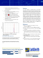
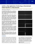
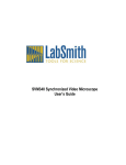
Lab-on-a-Chip Application: Field Amplified Sample
Stacking (FASS) for Sample Concentration in a
Nanochannel
Elizaveta Davies, Lesa Bishop, Adam Lucio, Jackson Travis del Bonis-O’Donnell, Sumita Pennathur, University of California, Santa
Barbara; Yolanda Fintschenko, LabSmith, Inc.
A ubiquitous problem in analytical chemistry is the push to
increase signal-to-noise (S/N) and to lower the limits of
detection (LOD) for many sample separation methods. Low
S/N is typically due to the inherent low concentration of
the sample in the system and the band-broadening of the
sample in dead volumes of the analytical system. The
microfluidic chip platform can address both these issues.
Microfluidic channel networks have an advantage over
conventional fluidics for chemical separations by
eliminating dead volume found in tubing-based
connections. This can be exploited when using electric field
manipulation for increasing the concentration of sample in
the injected volume. Field Amplified Sample Stacking
(FASS) takes advantage of the effect of applying an electric
field across a conductivity gradient in the buffer. The
amplification gained by FASS is even more efficient when
coupled with a microfluidic chip, due to channel integration
that minimizes dead volumes. In this application note, we
will describe the procedure for FASS using commerical
LabSmith equipment.
Introduction
Field-amplified sample stacking, or FASS, first described in the late
1
1970s for traditional capillary electrophoresis applications , has
2
been optimized in the 1990s through the present for applications
from traditional capillary zone electrophoresis to nanofluidic
3
separations . The stacking effect in a fluid-filled channel is caused
by an electric field gradient created when the background
electrolyte in the sample is lower in conductivity than the buffer, as
shown in Figure 1. The charged sample of interest is at least three
orders of magnitude lower than the electrolyte, so the fluid’s
electrical conductivity is determined solely by the electrolyte in the
sample. When an electric field is applied across the channel, it has a
step change increase within the low conductivity region due to
increased resistance. This results in a higher electrophoretic
velocity of the sample ions within the low conductivity region
relative to the high conductivity buffer. Therefore, the sample ions
quickly leave the low conductivity region and slow upon reaching
the high conductivity region. This causes the sample to occupy less
volume as it is accelerated into this boundary, increasing
concentration in a narrow band. The term “stacking” refers to the
finite increase in sample ion concentration across the interface
between different conductivities.
Figure 1. FASS Principle Schematic. Top: No stacking. Conductivity
in regions A, B and C are equivalent. The electric field is the same
across all regions of the channel. Bottom: FASS. Conductivity is A
=C>>B. The electric field is greater in sample region B. Sample
stacking occurs where the electrophoretic velocity (UEPHORETIC)
increases dramatically at the region of the border between A and
B, but the electroosmotic flow (EOF) is still stronger and drags
everything, including the concentrated sample plug (yellow), to
the cathode.
Figure 1 shows this schematically for a negatively charged sample
ion. This concentration factor can be controlled and preserved
using a microfluidic chip. The experiment described below is a
classic tool that has useful applications and teaches students and
new microfluidics practitioners about the effect of electric fields,
controlling the injection step to preserve stacking by minimizing
dilution due to dead volume, and the effects of these conditions on
the subsequent separation. Coupled with a gated-injection, this
experiment is a powerful illustration of electrophoretic,
electrokinetic, and microfluidic principles.
Control of electric fields, timing, and inverted fluorescent
microscopy and data recording is required for FASS to succeed. The
HVS448 programmable eight-channel high voltage power supply
controls eight ports which can be used for up to two simultaneous
on-chip FASS experiments. The SVM340 Synchronized Video
Microscope is an inverted fluorescence microscope that is used to
image the injection itself and provide raw data for the
measurement of the downstream separated sample plug. The
HVS448 Sequence™ software gives the user fully-automated
control of the electric field program applied to each electrode.
These features have been employed by Davies, Lucio, Bishop, Del
Bonis O-Donnell, and Pennathur at University of California, Santa
Barbara, to successfully produce a teaching laboratory exercise,
training students to perform and analyze the results of FASS on a
chemical separation.
GOAL: The novice will learn how to create an electric field gradient
to control sample stacking by varying buffer conditions, electric
field strengths, and injection times. Users can use either a gated or
4
pinched injection to load the sample. For operating guidelines with
LabSmith equipment, refer to the gated injection or pinched
5,6
injection application notes to optimize their injection conditions.
High-Voltage Power Supply (HVS448) Setup
1.
2.
FASS Experimental Set-Up
Equipment and Materials

LabSmith SVM340 Synchronized Video Microscope with
uScope™ software
o SVM340 Black and White Camera Module
o Blue Illuminator
o 10X DIN 0.25 objective
o 515 nm Long-pass filter

LabSmith HVS448 6000D High Voltage Sequencer with
Sequence™ software
o Platinum electrodes (4)
o Micro-Clip connectors
o High Voltage Cables

10-100 µL pipette with 100 µL pipette tips

0.2 µm solution filter

Particle-free wipes

Disposable nitrile gloves

Safety goggles
Glass cross-channel nanochip (Figure 2) with 250 nm deep x 7.5
µm wide channels ( Dolomite chip, http://www.dolomitemicrofluidics.com/en/design/custom-devices ).
Solutions

Buffer: 10 mM Phosphate buffer at pH ~7.2

Fluorescent Sample: 1 mM Phosphate buffer (pH ~7.2) with 1
mM sodium fluorescein

Deionized (DI) water (18 MΩ)

100 mM potassium hydroxide (KOH)
3.
Plug HVS448 into wall power and to computer via the RS232
port. Turn on the unit and launch the Sequence™ software.
Create a new Sequence file using the steps in Table 1 for
Sequence Steps A-F.
a. See the Using the Sequence Wizards to Create a
Sequence File section of the Sequence Users Manual (pp
13-17) for instruction on making a Simple Sequence
Wizard and Running a Sequence.
Note: The values in Table 1 were developed for use with a
specific chip geometry and buffer pH as described in the
Experimental Set-Up section. You will need to adjust the
voltages if using a different configuration.
Connect the high-voltage cables to the HVS448:
a. Turn off the HVS448 and remove the interlock (50 Ω
terminator) from the back of the unit to disable the high
voltage.
b. Plug high voltage cables A-D in channels HVA-HVD.
c. Install a microclip and platinum electrode on the labeled
end of each cable. Alternatively, press the electrode
directly into the end of the cable.
d. Follow the instructions in the Grounding the HVS4448
Channels section of the Sequence™ User’s Manual (pps.
11-12) to ground the unit.
Inverted Microscope (SVM340) and Chip Setup
1.
2.
3.
4.
5.
6.
Setup the SVM340 with a black & white camera module
installed with a 515 nm filter and a blue illuminator.
Plug the SVM340 into wall power, into the computer via the
RS232 port, and to the video capture card via USB port. Turn
on the unit.
Launch the uScope™ software and ensure you are viewing a
live video. See the uScope™ User’s Manual for instructions on
selecting the proper video settings.
Place your chip on the stainless steel microscope plate and
secure. Double-stick tape or magnets work well for holding
the chip on the stage (the plate is magnetic stainless).
Install reservoirs on the chip ports to allow the channels to be
filled with fluid and provide a place to insert the electrodes.
Adjust the X-Y and focus position of the stage to locate the
channel region of interest.
Filling the Chip
1.
2.
Figure 2. Diagram of Microfluidic Chip. Length of the channel W to
E is 35 mm +/- 0.30 mm; N to S is 10 mm +/- 0.30 mm.
Filter all solutions with a 0.2 µm filter.
Degas solutions by sonicating for 15 minutes in a container
with the cap loosely fitted on top.
Water fill (to clean and wet channels)
3. Use a 10ul pipette with disposable tips to fill the channel
reservoirs with DI water in the following order, see Fig. 2: W,
E, N, and S. Wait approximately 10 seconds between filling
each reservoir.
4. Adjust the microscope X-Y stage to inspect all channels for air
bubbles or particle contamination; flush chip to clean if
necessary.
5. Insert the electrodes connected to HV cables A-D in reservoirs
N, E, S, and W, respectively.
6. Run the loading step of the Sequence™ software:
WARNING: you are about to apply high voltage to the
channel. Read and follow safety precautions outline in
the HVS448 User’s Manual (Cautions and Warnings and
Grounding the HVS448 Channels sections of user’s manual
pps. 9-12) before proceeding.
a.
b.
c.
d.
e.
f.
WARNING: Ensure high voltage is disabled before handling
chip reservoirs.
12. Using a pipette, remove the buffer from the North (N)
reservoir and replace it with the fluorescent sample.
13. Run the Loading step (Step A) using the procedure outlined in
step 6, but with the fluorescent sample and buffer instead of
DI water.
a. Position the X-Y stage under the intersection of the
cross-channel to observe the fluorescent sample flowing
from the north to south channels. It should be an
obvious distinction from the east and west channels.
b. Ensure high voltage is disabled before handling chip
reservoirs.
Table 1. Values for 250 nm depth Dolomite chip
Install the interlock (50 Ω terminator) in the HVS448
back panel.
Turn on the HVS448 power button and ensure you are
working online (toggle the offline button if not).
In the Sequence™ software, click the Enable high
voltage output button.
Run the loading step of the sequence you previously
made by going to the menu bar and choosing
Actions>Run>Step A.
Run Loading step for at least 5 minutes.
After loading is complete,click Stop button, then click
the Disable high voltage output button.
WARNING: ALWAYS ensure high voltage is DISABLED before
handling chip reservoirs/electrodes.
KOH solution fill (to clean, expose, & ionize hydroxyls on channel
surface)
7. Pipette DI water from each reservoir. Rinse each reservoir
with the KOH solution by aspirating/dispensing into the well
(W->E->N->S) 4-5 times. Fill each reservoir with fresh KOH
solution.
8. Run the KOH Loading step (Step B) using the Sequence™
software for at least 5 minutes. Use the procedure outlined in
step 6.
WARNING: ALWAYS ensure high voltage is DISABLED before
handling chip reservoirs/electrodes.
Water rinse (to remove KOH to prevent reaction with buffer)
9. Rinse with DI water by repeating step 7 two times using DI
water instead of KOH.
Buffer and fluorescent sample fill
10. Replace solution with buffer, repeating step 7 using buffer
instead of KOH.
11. Run the Loading step (Step A) using the procedure outlined in
step 6, but using the buffer instead of DI water.
Step
VNorth
Voltages (V)
VEast
VSouth
VWest
A) Loading
828
1500
0
752
B) KOH Loading
276
500
0
251
C) Gating
1000
-3000
300
1000
D) 16 kV/m Injection
280
0
280
1000
E) 32 kV/m Injection
560
0
560
2000
F) 48 kV/m Injection
840
0
840
3000
Collecting Data
1.
2.
3.
4.
Move the X-Y stage at least 10 channel widths towards E to
avoid geometry effects.
Alternate the Gating Step (Step C) and an Injection Step (Step
D, E, or F) to create concentrated sample plugs.
Using the uScope™ software, record a video of the fluorescent
plug(s) passing through the monitored section of the channel.
The Intensity Probe feature of the uScope™ software can be
used to quantatively measure the concentration of the plugs.
a.
b.
c.
Click the Intensity Probe toolbar button
to highlight
the button.
With your mouse curser over the image, right click on the
mouse and select New Probe. Click on the image to draw
the outline of the probe. When the shape is defined
double click the mouse to close the polygon.
Once created, the probe can be moved by clicking and
holding the mouse button over the probe and dragging it
to the desired location. The shape of the probe can also
be modified by dragging the polygon points to create the
desired shape.
d.
5.
Intensity probe data displayed and recorded can be
selected by selecting the probe (left click), then right click
and select Properties.
To record probe data:
a. Choose File >Measurement File Naming to select how
the recorded data will be saved.
b. To begin recording choose File >Record, or click the
c.
d.
Start/Stop
toolbar button. If Autonaming is
selected, recording will begin immediately. Otherwise,
recording will begin after you name the file and click OK.
To end recording, choose File > Record or click the
Start/Stop button again.
Data can be opened in an Excel spreadsheet to plot
intensity versus time (Figure 3).
Summary
The critical challenge in controlling FASS is the selective
manipulation of the mass transport of the sample using an electric
field step gradient created by a difference in solution and sample
conductivities. This requires the control of different voltages at four
ports and the timing of the voltage switching as the injection is
made. The HVS448 can control up to two of these experiments
using all eight channels using the unique Sequence™ software . The
SVM340 is uniquely designed as an optical benchtop for
microfluidic experiments with isolation of the fluid and electrical
connections from the translatable optics below the experiment.
The SVM340 uScope™ software allows the user to take videos and
snapshots for processing later. uScope™ provides intensity probes
that create a software detection window that can be applied in real
time or post-processing video so users can obtain traditional
intensity vs. time plots of their experiment. This is particularly
useful for optimizing injection and run conditions for
electrophoretic and electrokinetic separations.
References
Figure 3. FASS Injection. Red: FASS Amplified Signal.
Blue: No amplification.
Vary Conditions, Analyze, Report Data
The following parameters can be varied to experimentally optimize
the conditions for stacking: conductivity difference between
sample buffer and separation buffer; injection time; electric field.
(1) Mikkers, F.E.P.; Everaerts, F.M.; Verheggen, Th. P.E.M. J.
Chromatogr. A 1994, 69, 11.
(2) Chien, R.L. and Burgi, D.S. Anal. Chem. 1992, 64, 1992, 489A.
(3) Sustarich, J.M.; Storey, B.D.; Pennathur, S. Physics of Fluids 2010,
22, 112003-1.
(4) Jacobson, S.C. and Culbertson, C.T. Microfluidics, Some Basics, in
Separation Methods in Microanalytical Systems, eds. J.P. Kutter
and Y. Fintschenko, CRC Taylor and Francis, Boca Raton, FL, 2006,
48.
(5) Fintschenko, Y. Making a Pinched Injection, LabSmith Application
Note #LSAPPS4, 2011.
(6) Davies, E.;Bishop, L., Lucio, A.; Pennathur, S.;Fintschenko, Y.
Making a Gated Injection, LabSmith Application Note LSAPPS5,
2011.
(7) Skoog, D. A., Holler, F. J.; Crouch, S.R. Principles of Instrumental
th
Analysis, 6 ed., Brooks/Cole Publishing, Belmont, CA, 2007.
Students should be able to predict the general trends, compare
their data to expected trends, and explain deviations where they
7
occur.
LabSmith Products Used in FASS Application
HVS448 High Voltage Sequencer with Sequence™ Software
HVC High Voltage Cables
SVM340 Fluorescence Microscope with uScope™ Software
Learn more at www labsmith.com.
6111 Southfront Rd. Suite E, Livermore, CA 94551
Phone (925) 292-5161 | Fax (925) 454-9487
www.labsmith.com | [email protected]
© 2011 LabSmith, Inc. LSAPPS6 – 9/11