Download loudness compensation of music in a car audio system

LOUDNESS COMPENSATION OF MUSIC IN A CAR AUDIO SYSTEM
Master Acoustics, 8th Semester, Spring 2012
12gr860:
-
Pablo Cervantes
Sebastian Prepelita
Regnar Bonde
Supervisor: Pablo Faundez Hoffmann
Department of Electronics Systems
Preface
1 PREFACE
This report is written by group 860 at 2.semester on the Acoustics Master program at the department of electronics
systems, Aalborg University, spring 2012.
Group members :
Pablo Cervantes
Sebastian Prepelita
Regnar Oxholm Bonde
Supervisor:
Pablo Faundez Hoffmann.
1.1 ACKNOWLEDGES
Before developing the project explanation, we’d like to thank Pablo Faundez Hoffmann, our supervisor, who provided
us help about the project conduction. Moreover, he took care of renting the university car used for measurements
and he was our driver when needed.
Thanks to Peter Dissing and Claus Vestergaard Skipper for help regarding equipment which could be used in the car.
12V supply.
Thanks to the IT staff members, for assisting us on problems regarding to the group folder for storage, and for the
SVN.
Finally, thanks to Aalborg University for giving us the opportunity to discover a school system, and a relevant
experience for international experience.
1
Preface
1.2 READING GUIDE
The project documentation is divided into the following three parts:
Report: is the main documentation for the project and is chronologically composed. To understand the project it is
recommended to read this part. The report is divided into several smaller parts. A problem formulation part where the
problem is described and requirements and limits for the project are chosen. An analysis part where theory and
practical issues are discussed and analyzed. An implementation part where the development and implementation of
the problem are described. And finally a conclusion. If a fast overview is needed read the introduction, problem
formulation and the conclusion.
Appendices: include further and deeper information about the project. However the appendices are not mandatory
for the project understanding. Measurement journals, references etc. are placed in the appendices
DVD: includes Python and Matlab codes, recordings, equipment-datasheets etc. Documents which have low
importance for the project or data which are not printable. The DVD does also contain the report and the appendices
as PDF.
References for used material are written in squared brackets with author surname and year of publication. The same
is applicable for webpages but only the page name is in the brackets. A total list of references is available in 9.4
Appendix D. References. References to codes and other files on the DVD are written in italic.
1.3 PROGRAMMING LANGUAGE (MATLAB VS. PYTHON)
The main programming language used in this project is Python. Python is a high level programming language with a lot
of possibilities and some similarities to Matlab. The main reason why we chose Python as the main programming
language over Matlab was due to the possibility to choose a part of this project to be a mini-project in the course
Scientific computing and sensor modeling. The programming language for the mini-project in this course had to be
Python and to avoid a mix of Python and Matlab code, which would make an on-line system difficult to implement, in
this project we therefore decided to use Python. Also, Matlab is not intended for high performance computing,
making Python a better choice for multithreading and multiprocessing that can gain even more from GPU computing –
a field where Matlab still has some compatibility issues.
2
Preface
2 CONTENT
1
Preface ........................................................................................................................................................................ 1
1.1
Acknowledges ..................................................................................................................................................... 1
1.2
Reading guide ..................................................................................................................................................... 2
1.3
Programming language (Matlab vs. Python) ...................................................................................................... 2
3
Introduction ................................................................................................................................................................ 5
4
Problem formulation .................................................................................................................................................. 6
5
4.1
Objective ............................................................................................................................................................. 6
4.2
Specifications ...................................................................................................................................................... 6
4.3
Limitations .......................................................................................................................................................... 7
Analysis ....................................................................................................................................................................... 8
5.1
Introduction ........................................................................................................................................................ 8
5.2
Music in reference condition .............................................................................................................................. 8
5.3
Measurement setup ........................................................................................................................................... 9
5.4
Noise in the car ................................................................................................................................................. 11
5.4.1
Recording positions .................................................................................................................................... 11
5.4.2
Velocities ..................................................................................................................................................... 11
5.4.3
Octave band analysis .................................................................................................................................. 12
5.4.4
Results and analyzing .................................................................................................................................. 12
5.4.5
Conclusions ................................................................................................................................................. 17
5.5
Car transfer functions ....................................................................................................................................... 18
5.5.1
5.6
Loudness ........................................................................................................................................................... 23
5.6.1
Loudness models ........................................................................................................................................ 23
5.6.2
Partial masking of loudness ........................................................................................................................ 24
5.7
6
Transfer function processing ...................................................................................................................... 18
Chosen program material ................................................................................................................................. 25
Implementation ........................................................................................................................................................ 26
6.1
Introduction ...................................................................................................................................................... 26
6.1.1
6.2
The ideas ..................................................................................................................................................... 26
Noise extraction ................................................................................................................................................ 28
6.2.1
Testing for reliability ................................................................................................................................... 28
6.2.2
Analysis of data ........................................................................................................................................... 29
6.2.3
Decreasing slice size .................................................................................................................................... 31
6.2.4
Noise extraction .......................................................................................................................................... 32
6.2.5
Microphone position for noise estimation ................................................................................................. 39
3
Preface
6.3
Loudness and masking compensation .............................................................................................................. 44
6.3.1
Signal to diffuse field transfer function ...................................................................................................... 45
6.3.2
Diffuse field to cochlea transfer function ................................................................................................... 45
6.3.3
Noise threshold levels ................................................................................................................................. 55
6.3.4
Signal threshold level .................................................................................................................................. 57
6.3.5
Hearing threshold ....................................................................................................................................... 58
6.3.6
Gain calculations ......................................................................................................................................... 59
6.3.7
Gain smoothing ........................................................................................................................................... 61
6.3.8
Octave band filter and equalizer ................................................................................................................. 65
6.4
Total implementation of the loudness compensation system in Python ......................................................... 69
6.4.1
7
8
9
Inside the main application ......................................................................................................................... 70
Test and results ......................................................................................................................................................... 73
7.1
Online test of loudness compensation system in laboratory ........................................................................... 73
7.2
Online test of loudness compensation system in car ....................................................................................... 74
Conclusion ................................................................................................................................................................ 75
8.1
The loudness compensation system and it’s behavior ..................................................................................... 75
8.2
Objective judgment of the loudness compensation system ............................................................................. 77
8.3
Subjective judgment of the loudness compensation system ........................................................................... 77
8.4
Further development ........................................................................................................................................ 78
8.4.1
Increasing the amount of octave bands ..................................................................................................... 78
8.4.2
Investigate other loudness models ............................................................................................................. 78
8.4.3
Apply temporal, forward and backward masking. ...................................................................................... 78
8.4.4
System improvements ................................................................................................................................ 79
8.4.5
Improved noise estimation system ............................................................................................................. 79
Appendices ............................................................................................................................................................... 80
9.1
Appendix A. Measurement journals ................................................................................................................. 80
9.1.1
Verification of measurement setup ............................................................................................................ 80
9.1.2
Car transfer function measurements .......................................................................................................... 82
9.1.3
Noise measurements in car ........................................................................................................................ 85
9.1.4
Measuring final result ................................................................................................................................. 88
9.2
Appendix B. DVD contents ................................................................................................................................ 91
9.3
Appendix C. Dictionary...................................................................................................................................... 93
9.4
Appendix D. References .................................................................................................................................... 95
4
Introduction
3 INTRODUCTION
In today’s fast-moving world, the car is becoming little by little the main place people listen to music, to audiobooks or
good old radio. Despite many advantages that a car can offer compared to a standard listening room while stuck in a
traffic jam, things get a little complicated when it comes to listening to various playback materials while average
driving velocities becomes contemporary relevant.
As the vehicle’s velocity increases, various indispensable noise sources increase in loudness, making the playback
material from partly unhearable to indistinguishable. Sound generated by the car’s engine and tires, by wind friction
with the car body, by road bumps or simply road type increase so much with velocity that from one point on the
material played through the car’s sound system turns out to be quite different than what was initially intended. With
some bad weather added to this, the listener has to take action like turning up the volume which will become a strong
impediment to many normal car activities: chatting, speaking on the phone etc.
The noise generated while travelling will have most of its energy concentrated at low frequencies, making the middle
and higher frequencies not audible. Although one would expect only some frequencies to disappear, the
psychoacoustical effect of masking makes the masked frequency band even larger. As the velocity increases, the
energy starts moving up in frequency and with enough ‘care’ by the user, car and environment the sound inside the
car will become pure noise – usually unpleasant to listeners. This can transform travelling by car into an unpleasant,
stressful and unhealthy environment.
An expensive solution would be a better isolation of the car. Another approach would be to compensate for such
adverse sound companions by adjustments in the playback material in such a way that it will not be masked by the
described noise and it will not affect the expected normal activities in what has become today an indispensable
comfort of our society.
5
Problem formulation
4 PROBLEM FORMULATION
4.1 OBJECTIVE
The objective of this project is to investigate how to restore the original apparent loudness of music material when
listening in the presence of background noise in the car. The original apparent loudness is the same quantity (an
attribute of the auditory sensation to rate sounds from quiet to loud) on a certain scale as in a chosen reference
condition [Moore, 2012]. In order to do this, different signal processing techniques, human sound perception and
loudness models will be studied and finally we develop a system able to compensate for loudness of music played in a
car and evaluate the performance of such system e.g. loudness compensation system. To be able to listen to the
performance of this system, a recording of the loudness compensation system in action, in a car, will be performed
with an artificial head. This gives the possibility to subjectively judge and analyze the system behavior including the
applied loudness model, by only using headphones and the binaural recording through binaural reproduction. Because
we want to develop a loudness compensation system, analysis and investigations is done from implementation point
of view and implementation is therefore also a part in this report. We need the loudness compensation system for
best possible analyzing and judgment of how to restore the original apparent of loudness. A loudness model alone or
other theory will be hard to judge and analyze if they are just formulas or a piece of code.
4.2 SPECIFICATIONS
Even though the main objective for this project is to investigate how to restore the original apparent loudness of
music, we have chosen to have big focus on development of a loudness compensation system to be able to better
understand and evaluate the mentioned objective. Before defining the specification we define some general terms
that will be referred to throughout the report:

Playback signal represents the signal played through the tested car-audio system

Program material represents wave-file containing various chosen playback signals mixed together used for
testing the loudness compensation system to be developed

Period represents a part (of approximate length of 30 s) in the program material containing the same type of
material (e.g. pink noise, speech, electronic music etc.)
Specifications for the loudness compensation system have been decided. These are:

The loudness of playback signal shall sound equal no matter the noise.

The system shall allow user settings e.g. volume and equalizer settings. If the user likes loud bass levels, the
loudness compensation should not overrule this user behavior.

The developed system shall be able to perform online loudness compensation in a car. Not only simulations.
6
Problem formulation
4.3 LIMITATIONS
Due to a limited time-period, man-hours, and for simplifying (easier analyzing of results), project-limits are introduced.
The following points will be covered / not covered by the project and project-report.

The loudness compensation system will only be optimized for one certain listening position even though
there is room for more than one person/listener in the car. The listener position is necessarily not the driver
position and will be chosen from a practical point of view.

Only 2 speakers will be used even though new cars typical have 4 or more. The 2 speakers are not necessarily
the speakers build into the car. They can also be speakers from the laboratory. Which speakers we are using
depends on the audio system in the rented car and practical issues.

Noise cancelation of any kind will not be included in the loudness compensation system and not discussed in
the report.

Equalization to flatten the response from the speakers and car cabin will not be implemented in the loudness
compensation system and not discussed in the report.

Cabin changes to improve the cabin acoustic or noise isolation will not be carried out.
7
Analysis
5 ANALYSIS
5.1 INTRODUCTION
Before development of the loudness compensation system, different investigations and analysis are needed. This part
will therefore cover investigations and analysis of theory and practical issues to support the development of a
loudness compensation system described later in this report. Analysis of loudness and loudness models, which can be
used to predict the perceived loudness and therefore be used to restore the original apparent loudness of music
presence in noise, will also be analyzed.
5.2 MUSIC IN REFERENCE CONDITION
Various playback signals like cd, radio, etc. are intended to be played at reference conditions or close e.g. in a living
room. The playback signal is often mixed in a studio with reference conditions and to have the same experience and
sound it is recommended to play it in the same conditions or close to. From [IEC 60268-13] a reference conditions can
be obtained using following steps:

To ensure uniform distribution of low frequency eigen tones, the room dimension ratios should be
2
2
(W/H)≤(L/H)≤(4.5(W/H)-4), where L is length, H is height and W is width. The preferred size is 25m to 40m .

The reverberation time should be between 0.3 s and 0.6 s for 200-4000Hz sounds. The ceiling should be
mostly reflective, the floor mostly absorbent and additional absorption material should be uniform
distributed.

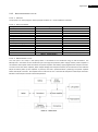
The background noise should in no circumstances exceed the levels in Table 5.1.
Frequency [Hz]
Max SPL [dB ref to 20µPa]
31.5
65
63
47
125
35
250
26
500
20
1000
15
2000
12
4000
9
8000
7
TABLE 5.1 - MAXIMUM BACKGROUND NOISE SPL FOR REFERENCE CONDITION.

The distance between the speakers should be between 2m and 3.5m pointing towards the listening position
with treble units at ear level. The listener should be positioned symmetric in the room and 2.5m to 3.5m
away from the line connecting the speakers. No listener should be placed closer than 1m to a wall and 2m to
a speaker.
In the case the playback signal is played in a car, the reference conditions are almost not existent and impossible to
fulfill. The following will give rise to problems in the car:

Reverberation time and reflections due to non-uniform distribution of absorption material. Soft seats and
panels and hard windows.

Comb filtering and strange frequency response due to the small cabin.

Speaker / listener position. None of the distances can be obtained.

Noise floor.
The first 3 points are due to the cabin size and cabin arrangement and because of the limits chosen for this project
these will not be discussed further. We will instead focus on point 4 which is due to noise from engine, wind, etc.
8
Analysis
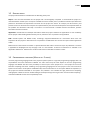
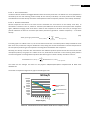
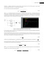
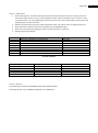
5.3 MEASUREMENT SETUP
In order to do measurements in the car we need a setup which consists of mainly an amplifier, speakers, microphone,
a sound source and various equipment, needed for specific measurements. For the speakers and amplifier we could
use the car audio system which is already installed in the car or we could add our own setup. The advantages of using
the existing car audio system is that everything what we need is installed in the car and ready for use but the
disadvantages is that we don’t know the system before we have the car. It could be too bad for this project point of
view. The amplifier maybe introduces phase and frequency changes and the speakers maybe have a bad frequency
response or it will be difficult / impossible to interface a computer with the car’s audio system. Due to that, we
decided to add our own system.
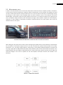
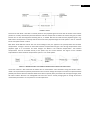
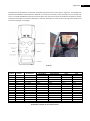
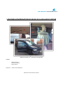
FIGURE 5.1 - THE CAR AND ITS AUDIO SYSTEM. IT SEEMS THAT THE DECISION TO ADD OUR OWN AMPLIFIER AND SPEAKERS WAS A GOOD IDEA.
THE EXISTING CAR AUDIO SYSTEM ONLY HAS A FM RECEIVER AND A TAPE PLAYER. NO AUX INPUTS.
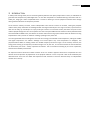
When adding our own system we are able to control everything and validate that our system behaves as expected but
we are limited to a 12V power supply and we are not able to position the speakers where speakers are normally
positioned in a car. The power supply problem is solved using as much battery powered equipment as possible. We
are using a laptop with an USB powered soundcard and the phantom power for the measurement microphone is also
battery powered. Only the amplifier needs 230V but this is easily solved using a DC/AC converter (12V to 230V). We
could have bought a new 12V car amplifier but the used amplifier and DC/AC converter was available in the
laboratory.
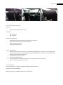
FIGURE 5.2 - THE BASIC SETUP IN THE CAR.
9
Analysis
The chosen speakers were B&W DM601 S2. They are chosen on compromise between size and ability to produce low
frequencies. They fit into the car and a -6dB cutoff frequency at 50Hz is acceptable for a speaker of this size. The
chosen microphone is B&K 4134 which is a pressure field microphone and chosen because the car cabin is assumed to
be a diffuse field and because of its frequency range. It is able to measure frequencies between 4Hz and 20KHz which
covers the frequencies we are focused on (20Hz to 20Khz). Frequencies we are able to hear. All used equipment
including serial numbers are listed in 9.1 Appendix A. Measurement journals.
To validate the electrical part of our setup we have measured the impulse response when the amplifier output is
looped to the microphone input in 9.1.1 Verification of measurement setup. We expect the phase and frequency
response to be flat and the impulse response to be close to a dirac delta. This holds true for this setup.
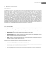
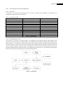
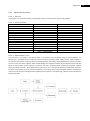
All equipment except speakers, microphone and laptop are placed in the trunk of the car. The speakers are placed on
the backseats and the listener in between. The used car has actually 3 rows of seat where cars normally only have 2.
To handle this difference the second row of seats in the used car was not used. The speaker and listener position was
chosen to satisfy the speaker and listener position in reference condition best possible. The speakers were placed
symmetrically to the listener in the cabin and the speakers pointing at the listener ears. The microphone does not
have a certain position. This is because different positions will be analyzed later in the report. Temperatures and
humidity is not taken into account.
FIGURE 5.3 - EQUIPMENT POSITIONS IN THE CAR.
10
Analysis
5.4 NOISE IN THE CAR
This section is about the study of the behavior of the noise in different scenarios. It is clear that noise from different
sources (wind, engine, traffic, etc.) is present during driving activity. We want to know how the noise is distributed
1
and the SPL to know which frequencies of the playback signal we can expect to be masked or have decreased
loudness while driving.
In the loudness compensation system we want to develop and described in chapter 6 Implementation, one recording
position should be chosen. Since the recorded signal will be used solely for noise estimation, the positioning of the
microphone should best estimate the noise in the car (as close as possible to noise at the listener position) and should
be robust enough to playback signal and car-velocity.
The noise is recorded at 4 positions (9.1.3 Noise measurements in car). The noise is extracted from the silence period
of the program material (5.7 Chosen program material), recorded in the measurement session and analyzed with
python scripts. These scripts are included in the Python module DVD\Code\Python codes\_Analysis\Noise_Analysis.py.
The analysis of the measured noise will be based on the different recoding positions and car velocity.
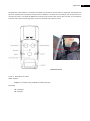
5.4.1 RECORDING POSITIONS
Following recording position was chosen.

Back: This position is located behind the listener’s head. The aim of choosing this position is to study if we
have a good signal to noise ratio, considering the signal (desired signal) as the noise, and the playback signal
would be considered as noise signal. This will maybe improve the noise extraction.

Front: This position is located in the middle and top of the car. A preferred position from a practical point of
view if a loudness compensation system should be permanent implemented in a car.

Chest Level: This position has been chosen mainly for transfer functions purposes (knowledge about how
transfer functions changes depending on the position of the microphone). Noise has been studied in this
position as well, in order to have a better knowledge of this scenario.

Ear Level: This position probably is the closest one to the reality in terms of perception, but in the other hand
it is also the less practical. Because a microphone for recording has to be located in the car, this position is
not possible in a real system. The purpose of this position is to study the variability of the noise between this
position, which is the more realistic, and any possible position that could be implemented in a real system.
5.4.2 VELOCITIES
Several different car velocities for each position have been tested. Changes in the behavior of the noise due to the
car’s velocities are studied. The chosen velocities are 50Km/h, 80Km/h, 110Km/h. These represent the most common
used velocities while driving inside cities, roads outside cities and highways.
1
Ref to 20µPa and applies to all following SPLs.
11
Analysis
5.4.3 OCTAVE BAND ANALYSIS
The noise analysis is done in octave bands to best fit other parts of the project. Some parts in the loudness and
masking analysis later are analyzed using octave bands and parts of the implementation will be done in octave bands.
It is there reasonable to study the noise behavior with the same frequency representation technique.
Besides
Python
module DVD\Code\Python codes\_Analysis\Noise_Analysis.py, module DVD\Code\Python
codes\BandAnalysis\Band_Analysis.py has been used in this analysis (6.3.8 Octave band filter and equalizer). An octave
band bank of filters is applied to the measured signals. Afterwards the signal is converted from digital units to Pascals
(6.3.8.2 Converting from DU to Pa). For each filtered signal an RMS value is computed and converted to dB re 20µPa.
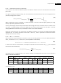
5.4.4 RESULTS AND ANALYZING
The results will be shown depending on the parameters: velocity and position. First we compare the noise at different
velocities for a certain microphone position and next we compare the noise at different microphone positions at a
certain velocity.
5.4.4.1 P OSITION B ACK
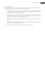
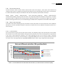
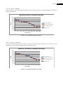
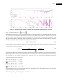
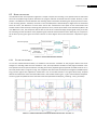
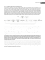
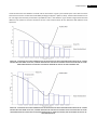
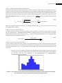
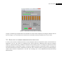
As it can be seen from Figure 5.4 the noise levels increases in all frequency range as the velocity does. If we consider
the noise floor as the noise measured when the engine was turned off, we can see how the engine has a big influence
in the noise at low frequencies especially in the range (125-500 Hz). We can see how this range is increasing
proportionally with the velocity, and how frequency range (1000-4000Hz) start to be an important influence when the
car start to move. Very high frequency range (8000-16000Hz) doesn’t suffer a “big” change with velocity changes.
SPL (dB)
Noise at different velocities. Mic position-Back
100,0
90,0
80,0
70,0
60,0
50,0
40,0
30,0
20,0
10,0
0,0
Noise Car_Back_No_Motor
Noise Car_Back_0
Noise Car_Back_50
Noise Car_Back_80
Noise Car_Back_110
31
63
125
250
500
1000 2000 4000 8000 16000
Frequency (Hz)
FIGURE 5.4 - OCTAVE BANDS NOISE LEVELS MEASURED IN BACK POSITION. 0, 50, 80 AND 110 REFER TO CAR VELOCITIES [KM/H].
12
Analysis
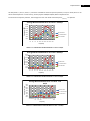
5.4.4.2 P OSITION F RONT
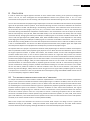
As it can be seen from Figure 5.5, a very similar interpretation to position back scenario could be done. Differences in
SPL are much higher in low frequencies (around 35-40 dB from noise floor to 110 km/h) when parameter velocity is
varied. We can see an important boost in the frequency range of 125-500Hz when the engine is turned on, and not
very important changes in level of SPL are seen in high frequencies.
Noise at different velocities. Mic position-Front
100,0
90,0
80,0
SPL (dB)
70,0
60,0
Noise Car_Front_Mic_No_Motor
50,0
Noise Car_Front_mic_0
40,0
Noise Car_Front_mic_50
30,0
Noise Car_Front_mic_80
20,0
Noise Car_Front_mic_110
10,0
0,0
31
63
125
250
500 1000 2000 4000 8000 16000
Frequency (Hz)
FIGURE 5.5 - OCTAVE BANDS NOISE LEVELS MEASURED IN FRONT POSITION. 0, 50, 80 AND 110 REFER TO CAR VELOCITIES [KM/H].
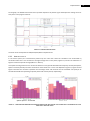
5.4.4.3 P OSITION CHEST LEVEL
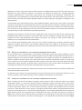
No measurements at 0 km/h were done for this position. As can be seen from Figure 5.6, the levels in the lower part
of the frequency range studied present similar levels, a fact which can be understood as a certain “independence”
from velocity. Also it can be observed an important change in SPL at middle frequencies (1000-4000 Hz).
Noise at different velocities. Mic position-Chest
90,0
80,0
70,0
SPL (dB)
60,0
50,0
Noise_Chest_level_50
40,0
Noise_Chest_level_80
30,0
Noise_Chest_level_110
20,0
10,0
0,0
31
63
125
250
500
1000 2000 4000 8000 16000
Frequency (Hz)
FIGURE 5.6 - OCTAVE BANDS NOISE LEVELS MEASURED IN CHEST LEVEL POSITION. 50, 80 AND 110 REFER TO CAR VELOCITIES [KM/H].
13
Analysis
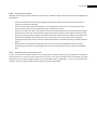
5.4.4.4 P OSITION EAR LEVEL
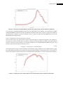
The behavior of the noise at this position is very similar to the chest level position. It can be seen how for low
frequencies (31-63Hz) the SPL are almost the same. At this position a bigger dependence from velocity can be seen in
a wider spectrum range. Values in high frequencies (8000-16000Hz) present small changes with different velocities.
Noise at different velocities. Mic position-Ear Level
90,0
80,0
70,0
SPL (dB)
60,0
50,0
Noise_Ear_50
40,0
Noise_Ear_80
30,0
Noise_Ear_110
20,0
10,0
0,0
31
63
125
250
500
1000
2000
4000
8000
16000
Frequency (Hz)
FIGURE 5.7 - OCTAVE BANDS NOISE LEVELS MEASURED IN EAR LEVEL POSITION. 50, 80 AND 110 REFER TO CAR VELOCITIES [KM/H].
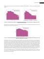
5.4.4.5 V ELOCITY : 0 K M / H . N O ENGINE
This measurement was done just in two different positions. From Figure 5.8 we can see how the noise levels with no
movement of the car and no engine are slightly higher in low frequencies. A big difference can be observed in the
frequency range of 250-2000 Hz and very similar values in high frequencies (4000-16000Hz). It should be mentioned
that the difference between the two measurements is expected because of the variability of the environmental
conditions. While the engine is running we don’t expect such variability due to the constant noise coming from it.
0 Km/h No Motor
60,0
50,0
SPL (dB)
40,0
30,0
Noise Car_Back_No_Motor
Noise Car_Front_Mic_No_Motor
20,0
10,0
0,0
Frequency (Hz)
FIGURE 5.8 - OCTAVE BANDS NOISE LEVELS AT 0 KM/H NO ENGINE.
14
Analysis
5.4.4.6 V ELOCITY : 0 K M / H . E NGINE ON
As can be seen from Figure 5.9, the SPL values are very similar in both positions when the engine is turned on. It is
worth to mention the predominance of the low frequencies in the noise level as was expected. This measurement was
done just in two different positions.
Noise at 0 km/h. Different Positions
80,0
70,0
60,0
SPL (dB)
50,0
40,0
Noise Car_Back_0
Noise Car_Front_mic_0
30,0
20,0
10,0
0,0
31
63
125
250
500
1000
2000
4000
8000 16000
Frequency (Hz)
FIGURE 5.9 - OCTAVE BANDS NOISE LEVELS AT 0 KM/H. ENGINE ON.
5.4.4.7 V ELOCITY : 50 K M / H
From Figure 5.10 very similar values for all positions at this position is observed. It can be seen how the noisiest
position is the back position. Also we can observe how chest and ear level positions have slightly smaller values,
probably due to the absorption of the listener.
Noise at 50 km/h. Different Positions
100,0
90,0
80,0
70,0
SPL (dB)
60,0
Noise Car_Back_50
50,0
Noise Car_Front_mic_50
40,0
Noise_Chest_level_50
Noise_Ear_50
30,0
20,0
10,0
0,0
31
63
125
250
500 1000 2000 4000 8000 16000
Frequency (Hz)
FIGURE 5.10 - OCTAVE BANDS NOISE LEVELS AT 50 KM/H.
15
Analysis
5.4.4.8 V ELOCITY : 80 K M / H
In this case we can see a higher difference between the back position and the rest, with SPL differences around 6-8
dBs in low frequencies.
Noise at 80 km/h. Different Positions
SPL (dB)
100,0
90,0
80,0
70,0
60,0
50,0
40,0
30,0
20,0
10,0
0,0
Noise Car_Back_80
Noise Car_Front_mic_80
Noise_Chest_level_80
Noise_Ear_80
31
63
125
250
500
1000 2000 4000 8000 16000
Frequency (Hz)
FIGURE 5.11 - OCTAVE BANDS NOISE LEVELS AT 80 KM/H.
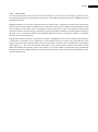
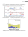
5.4.4.9 V ELOCITY : 110 K M / H
As can be seen from Figure 5.12, the behavior of the noise at 80 Km/h and 110 Km/h is very similar. The only
difference is a little increasing in the SPL values in all frequency range.
SPL (dB)
Noise at 110 km/h. Different Positions
100,0
90,0
80,0
70,0
60,0
50,0
40,0
30,0
20,0
10,0
0,0
Noise Car_Back_110
Noise Car_Front_mic_110
Noise_Chest_level_110
Noise_Ear_110
31
63
125
250
500 1000 2000 4000 8000 16000
Frequency (Hz)
FIGURE 5.12 - OCTAVE BANDS NOISE LEVELS AT 110 KM/H.
16
Analysis
5.4.5 CONCLUSIONS
From the previous section some conclusions about the behavior of the noise can be extracted. In general it can be
seen that the low frequencies (31-250 Hz) are much higher than middle and high frequencies for all different velocities
and different positions.
Regarding velocity, it can be seen in general and for all positions that, as expected, the noise levels increase with
velocity. The amount of energy in low frequencies is much more important than in middle and high frequencies, rising
up to 90 dB SPL in some cases. Also it is important to mention that values in SPL in the range (31.5-125 Hz) don’t
change too much for velocities 50, 80, and 110 Km/h, generally the difference between 50 and 110 Km/h is about 2-5
dB. Due to this, an important masking of the playback signal by the noise is expected to happen in all different
velocities, thus in all driving activity.
Regarding the position parameter, it can be seen how there is a big difference in the noise at 0 Km/h when the engine
is turned off in all positions. As it is mentioned in 5.4.4.5 Velocity: 0 Km/h. No engine, the noise levels due to the
engine is higher than the noise coming from environment conditions, therefore such a big difference is not expected
while engine is on. Also it can be seen that back position is the noisiest position that has been tested. The SPL
differences between back position and the other positions is around 6-8 dBs in the frequency range (31-1000 Hz),
reaching in some cases 10 dBs of difference. Also it can be seen how SPL in front, ear level and chest position are very
close for a fixed velocity.
17
Analysis
5.5 CAR TRANSFER FUNCTIONS
For estimation of the noise, implementation of the loudness compensation system and possible simulation of the
system, a couple of transfer functions need to be measured. The transfer functions were done using the software
[Holmimpulse]. The measurement (for additional information, see 9.1.2 Car transfer function measurements) was
16
done using a logarithmic sine sweep of 2 samples.
We chose sweeps over MLS for several reasons [Müller & Massarini, 2001]:


Sweeps perform better when it comes to distortion (MLS signal has a square wave shape which cannot
be ‘tracked’ exactly by the loudspeaker) and time variance
Sweep measurement has a better signal-to-noise ratio than MLS, an important asset in our case because
we want to measure outside in a ‘quite’ noisy environment
16
The chosen length of the excitation signal was 2 samples for all transfer function measurement, which for a 44100
Hz sampling frequency represents 1486 ms – enough to capture the low frequency reverberations in a cabinet like a
car cabin. The recording was set to record an extra time of 1500 ms – again, more than enough for the high
frequencies’ reverberation time.
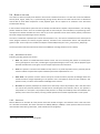
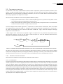
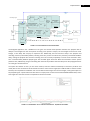
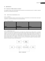
A block diagram of the measurement is depicted in Figure 5.13 (Out and In are processed and presented by the
[Holmimpulse] software). The test loop was done to check the system. For more and additional details about the
setup see 9.1.1 Verification of measurement setup.
Out
DU
D/A
V
Amp
V
Speakers
Car
Pa
Microphone
Test loop
In
DU
A/D
V
FIGURE 5.13 - TRANSFER FUNCTION MEASUREMENT OVERVIEW. THE TEST LOOP IS FOR VERIFICATION OF THE ELECTRICAL PART OF THE SETUP.
We begin the analysis based on the units presented by [Holmimpulse] software: transfer functions from DU (Digital
Units) to DU including the software processing (normalization, output type – float etc.). Then we will move on to the
desired transfer functions which are those that transform the playback DU and corresponding type to Pascals.
5.5.1 TRANSFER FUNCTION PROCESSING
Several decisions needed to be taken about the measured transfer function:
5.5.1.1 W INDOWING
Since the measurements exported from [Holmimpulse] software did not include the delay information in the sample
number (sample 0 was set to the highest peak of the impulse response, not to the time 0) and delay uncertainties
reside in different software while playback, the delay will be approximated and evaluated separately and the
windowing of the impulse response will start just as the exported impulse response raises above a certain threshold
from noise floor before highest peak. Algorithmically, this was done by searching for a number of consecutive samples
(used 10 consecutive samples) to be below a certain threshold (used 0.005 * highest_peak_of_IR(Impulse Response))
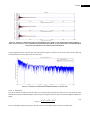
from the highest peak backwards. By visual inspection of the IR in the time domain we chose a fixed length for the
impulse response (set to 3000) samples – the impulse drops enough from maximum peak value in all measurements
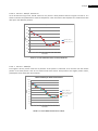
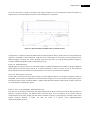
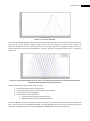
up to that point. This is depicted in Figure 5.14.
18
Analysis
FIGURE 5.14 - EXAMPLE OF A TRANSFER FUNCTION CUT (MEASUREMENTS 40,41,42 FROM 9.1.2 CAR TRANSFER FUNCTION MEASUREMENTS). Y
AXIS IS THE DIGITAL UNITS (DU) TO DU AS MEASURED BY THE [HOLMIMPULSE] SOFTWARE, THE BLUE LINE REPRESENTS THE MEASURED TIME IR
AND THE RED DOTS REPRESENT THE CUT SAMPLES FROM THE MEASURED IR.
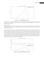
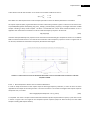
A typical logarithmic time response of the IR would look like Figure 5.15 and it can be seen that the chosen right side
cut (marked with a red star) falls inside the noise floor:
FIGURE 5.15 - EXAMPLE OF A LOGARITHM OF A TRANSFER FUNCTION. H IS THE IR IN TIME.
5.5.1.2 A VERAGING
In order to reduce the effect of the noise floor more measurements (three) were done for the same position of the
microphone and the windowed impulse responses were averaged in time for the same position [Müller & Massarini,
2001]:
[ ]
[ ]
[ ]
[ ]
Such an averaging is depicted in Figure 5.16 with a zoom around 1kHz (transfer function from DU to DU)
(5.1)
19
Analysis
FIGURE 5.16 - TRANSFER FUNCTION AVERAGING - AMPLITUDE AND PHASE RESPONSE FOR MEASUREMENT 37, 38 AND 39.
5.5.1.3 C ONVERTING IR
TO
The desired transfer function is from output DU to Pascals. For this requirement, the recorded DU (will be referred to
as ) measured in 9.1 Appendix A. Measurement journals for microphone placed inside the calibrator will be used to
convert any DU to its corresponding Pa value. Because this value was normalized to 1 (0.079 DU corresponds to -22.05
dB), care must be taken in the digital signal’s representation: the conversion will be done dependent on maximum
value of the signal with which the impulse response will be convoluted:
[ ]
[ ]
(5.2)
Since the signals will be loaded from wave files in 16-bit signed integer format (with a maximum of 32767), the new
transfer function will be calculated as:
[ ]
[ ]
(
[ ]
(5.3)
)
Some tests were done to check if the new transfer function was reliable. The recording in one position (front position,
without engine) of the entire measurement signal was converted to Pascals (6.3.8.2 Converting from DU to Pa) and
was compared to the transfer function [ ] convolved with the measurement DVD\Measurements\Car
measurements\front mic no motor.wav:
max(recording_Pa) = 0.82Pa
RMS(recording_Pa) = 0.11Pa
min(recording_Pa) = -0.86Pa
max(raw_Wave*h_Pa) = 0.10Pa
RMS(raw_Wave*h_Pa) = 0.01Pa
min(raw_Wave*h_Pa) = -0.11Pa
Also, the RMS value (in Pa) of the noise floor (which can be measured in the 30 seconds of silence in the program
material, no engine running) was calculated:
RMS(noise_floor_recording_Pa) = 0.03Pa
20
Analysis
We know that the recording of the transfer function was done with the amplifier set on 0 dB and the recording of
playback material was done with the amplifier set on +20 dB. Calculating the dB difference between the RMS values
(
)
(
)
(5.4)
and taking into account that the two recordings (transfer function measurement and program material
measurements) were done in different days and both the software used and soundcard gains were changed, the
values seem reasonable. However, gain compensation will need to be done for noise extraction (to compensate for
the mentioned gain changes).
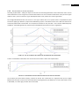
5.5.1.4 C OMPENSATE FOR MEASUREMENT DIFFERENCES GAIN AND DELAY
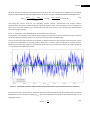
Front position: the recording in front position without engine (converted to Pa) was compared with program material
convoluted with the transfer function in the same position ( [ ] with calculated delay).
A zoom around 10 seconds shows that the simulation is delayed compared to the recording (Could have been caused
by delay from loudspeakers to recording position, differences in software when recording IR or playback material,
software processing of data, output vs input delay of sound chain etc.) and that the simulation has a higher amplitude
– as expected from the RMS values above:
FIGURE 5.17 - COMPARISON BETWEEN RECORDING AND SIMULATION AROUND SECOND 10 (FRONT MICROPHONE POSITION, ENGINE OFF).
To calculate the delay, we took the car dimensions [Parkers], [Internetautoguide] and calculated the distance from the
loudspeakers to each microphone position ( [ ] ) and then computed the time based on the speed of sound in air at
20 degrees Celsius, c.
[ ]
[ ]
(5.5)
21
Analysis
Then the corresponding number of zeroes was added in the beginning of the transfer function, based on the sampling
frequency when calculating the transfer function – 44100 samples/s:
[ ]
(5.6)
Therefore, the recording was delayed the corresponding number of samples and the transfer function modified by
15.35 dB to match the RMS value,
without the noise floor. The results after are plotted in Figure 5.18:
FIGURE 5.18 - COMPARISON BETWEEN RECORDING AND SIMULATION AROUND SECOND 10 - WITH GAIN AND DELAY COMPENSATION (FRONT
MICROPHONE POSITION, ENGINE OFF).
The above operations are done inside DVD\Codes\Python codes\Transfer_Functions\Compute_transfer_function.py
function readAndCompute_average_time_IR_FixedWindow(). Tests were done inside module DVD\Codes\Python
codes\Delaying\test_delay.py.
22
Analysis
5.6 LOUDNESS
An important part in this project is the understanding of loudness and masking and how it influences our hearing. Due
to our hearing organ we do not perceive loudness of a signal equal to its intensity. The perceived loudness depends on
frequency content and SPL of the signal, background noise, masking phenomena and maybe even more. The
mechanisms underlying the perception of loudness are not fully understood [Moore, 2012]. All these known
parameters which affect the loudness perception are combined in several different loudness models which can be
used to estimate the perceived loudness of a signal.
5.6.1 LOUDNESS MODELS
Different loudness models are, during the years, developed for use in practical situations. A basic structure for
loudness models, Figure 5.19, proposed by Moore [Moore, 2012], contains 4 blocks to calculate/estimate the
perceived loudness. First step is to filter the stimulus according to the outer and middle ear transfer functions and
then transform this to excitation pattern. The excitation pattern can be transformed to specific loudness and then the
perceived loudness can be calculated. This structure is used in the [ANSI S3.4-2005] for calculation of loudness of
stationary sounds.
FIGURE 5.19 - BASIS STRUCTURE FOR LOUDNESS MODELS[MOORE, 2012].
Because the mechanisms underlying the perception of loudness are not fully understood and the variation of ears and
hearing across different people, none of the models are able to calculate the true perceived loudness for one specific
person. Outer ears have different shapes and sizes as well as the middle and inner ears and due this and for sure other
factors, the perception of loudness will vary across different persons. The loudness models are therefore estimations
of perceived loudness for the average person. Some better than others, depending on input stimulus and purpose.
Some models are developed to estimate the loudness of stationery sounds and pure tones and if these are used to
estimate impulsive sounds with complex tones, they fail. The loudness models can be divided in two different groups
[Skovenborg, 2004]. A single band group, which estimate the loudness in one band and a multiband group, which
estimate the loudness in several bands. A single band loudness model could e.g. be Leq(A, B, C, D, M, RLB), where A, B,
C, D, M and RLB refers to different filter weightings, and LARM by TC electronics. A multiband loudness model could
e.g. be the model by Zwicker (ISO532B), Moore(ANSI S3.4-2005) and HEIMDAL by TC electronics. The multiband
loudness models are more complex than the single band because they divide the stimulus into several bands, applying
more filters and some of them even take into account masking. Hence, the multiband loudness models need more
computation than the single band loudness models. The question is now: Which model is the best to estimate the
loudness of music and speech, the signals which are typical played through a car audio system? [Skovenborg, 2004]
have analyzed how good different loudness models estimate the loudness of music and speech. These models are
then divided into 4 groups where group 1 is the best, Table 5.2.
Class
1
2
3
4
Models. (best-in-class listed first)
TC HEIMDAL, TC LARM
Leq(RLB), Leq(C), Leq(Lin)
Leq(B), PPM(50%), Zwicker-ISO, Zwicker&Fastl(95%)
Leq(D), Leq(A), Leq(M)
TABLE 5.2 - LOUDNESS MODELS ANALYZED BY [SKOVENBORG, 2004]. CLASS 1 ESTIMATES BEST THE LOUDNESS OF SPEECH AND MUSIC.
23
Analysis
All these models are able to estimate (some better than other) the perceived loudness. However, there is one
problem with the models for this project point of view. They don’t take noise into account which for sure affects how
loud a signal will be perceived. We want to know how loud the signal alone is perceived. Not the total loudness of
signal and noise, the partial masking of loudness.
5.6.2 PARTIAL MASKING OF LOUDNESS
Investigations and experiments for loudness of a signal in noisy environments are performed by [Lochner & Burger,
1961] and their results is used to create a function which describe the perceived loudness depends on noise and signal
intensity (5.7). They played a 1KHz pure tone in the presence of an octave band (700-1400 Hz) of random noise for
different test subjects. The pure tone + noise and the pure tone alone was played alternately through earphones for
periods of 1.3 sec and the test subject then had to adjust the level of the pure tone to match the level of pure tone
presence in noise. The results from these experiments were used to create and validate the function and later
experiments, by other authors, confirm their results [Florentine, Popper & Fay 2011]. The function is based on Stevens
power law. The loudness in sones for a signal in noise is:
(
)
(5.7)
Where I is the signal intensity and I0 is the threshold intensity for the noise. I0 is the threshold of the signal in the
presence of (any) noise (intensity of the signal at which it will just be masked by the noise). n is approximate 0.27
according to [Lochner & Burger, 1961] and k is a constant depending on the used units. In our case k is calculated to fit
the formula when the intensity levels are converted to SPL. The loudness in sones is then:
((
)
(
)
)
(5.8)
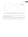
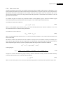
Where L is the signal SPL and L0 is the noise threshold level in dB. Figure 5.20 shows the function with different noise
threshold levels.
FIGURE 5.20 - PLOT OF PERCEIVED LOUDNESS OF A SIGNAL IN NOISE BASED ON THE MODEL BY [LOCHNER & BURGER 1961] (5.8). THE LOUDNESS
IS PLOTTED FOR NOISE THRESHOLD LEVELS AT 0, 20, 30 AND 40dB. FOR A NOISE THRESHOLD LEVEL AT 0dB, SIGNAL LEVELS AT 40dB
CORRESPOND TO 1 SONE.
Since the loudness model is based on 200-8000Hz pure tones as the signal, the function is not totally reliable for this
project. We want to predict the loudness for a complex signal (music) and this will maybe change the perceived
loudness depends on frequency contest in the signal. The width of noise does also affect how the loudness is
perceived [Florentine, Popper & Fay 2011]. If the noise has a width of a critical band, the loudness of the signal grows
more rapidly than the loudness function and if the noise is wider than an octave band, the loudness of the signal will
grow more slowly.
24
Analysis
5.7 CHOSEN PROGRAM MATERIAL
To analyze the behavior of loudness in a car we need some playback signals which are normally played in a car audio
system. These playback signals will be used during measurements, implementation of the loudness compensation
system and finally used for evaluation of the system. In order to choose some useful playback signals we have
followed recommendations given in the technical report [IEC 60268-13] part 13, listening tests on loudspeakers for
program material:

The chosen sounds should present differences between them, allowing the study of different important
sound perception aspects (dynamic range, frequency content, etc.)

At least six different sections should be included in the program material, covering from human speech, to
modern music.

High sound quality of the program material is needed.
Based on these recommendations, we have chosen the following materials. See Table 5.3. (Album titles in 9.4
Appendix D. References.)
Number
1
2
3
4
5
6
7
8
Music / sound source
Music for archimedes track 3 (0:00-0:30)
Silence
Music for archimedes track 4 and 5 (0:00 – 0:15)
Pavarotti – O sole mio (2:50 – 3:20)
Coldplay – Clocks (0:10 – 0:40)
System of a down – Chop suey (2:00 – 2:30)
th
Beethoven 5 symphony (0:00 – 0:30)
Trentemøller – Snowflake (2:41 - 3:12)
Genre/type
Pink noise
Silence
Speech
Opera
Pop rock
Hard Rock
Classical
Electronic
TABLE 5.3 – CHOSEN SOUND SOURCES FOR PROGRAM MATERIAL.
The first period is pink noise which is intended for level adjustments. It’s allows us to reproduce the levels in different
measurements using a SPL meter. The silence is necessary for noise floor recording, 9.1.3 Noise measurements in car.
The other sound sources are different kind of music and speech. The Pavarotti and Beethoven sounds sources are
highly dynamic compared to the Coldplay and System of a down sounds sources which does almost have no dynamic.
And Trentemøller is a sound source with huge information in the lowest frequencies.
Each part of the program material has a length of about 30 seconds and will have a fade in and fade out of 1 second.
They are individually normalized using DVD\Codes\Matlab codes\Loudness normalizing for wave files\Main.m based
on recommendation UIT-R BS.1770-2. This recommendation is based on LKFS (Loudness, K weighted, relative to
nominal full scale). The program material is normalized to -24dB LKFS which gives us headroom and possibility to gain
frequencies if needed (in e.g. the loudness compensation system).
The sound sources were put together with the software Adobe Audition CS5, one after each other and exported to
one mono 16bit file.DVD\Program material\Car_project_mixdown_MONO.wav. This allows us to play and repeat the
sound sources without adding unwanted changes.
The data was ripped and cut lossless.
25
Implementation
6 IMPLEMENTATION
6.1 INTRODUCTION
The implementation and solution part covers how the loudness compensation system is developed from scratch to
solution. The part will include different ideas, thoughts and how the solution is developed to have the desired
functionality. Investigation and analysis from chapter 5 Analysis is taken into account in this part and is used to form
and support the chosen solution.
The solution is divided into smaller parts which are developed and tested individually. This ensures better controlled
over the loudness compensation system and makes it easier to maintain and debug. It also gives the possibility to
parallel development. Finally all parts are put together.
6.1.1 THE IDEAS
Before development, different ideas were discussed and analyzed. Based on a brainstorm we ended up with 2
different ideas where the main difference is how to detect the noise in the car. The idea is from an early stage of the
project where we have a lack of knowledge to loudness, masking and loudness models. Due to that, different ideas for
the loudness compensation were therefore not possible. They are formed later in the project.
Figure 6.1 and Figure 6.2 Illustrate the ideas for the loudness compensation system and include both two blocks. A
loudness compensation block which will adjust the playback signal depending on playback signal and the noise. And a
noise block, which will estimate the noise in the car. Idea 1, Figure 6.1, using a noise model, controlled by some input
parameters, to calculated the noise in the car. The input parameters could e.g. be velocity, engine rpm,
accelerometers etc. However there are a lot of hard measurable parameters which also influences the noise in the car
and they are therefore not easy to take into account in a model. These parameters could e.g. be road type, tire type,
car type, car condition, weather conditions, traffic conditions, open/closed windows, open/closed sunroof, etc.
FIGURE 6.1 - IDEA 1.
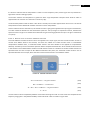
Idea 2, Figure 6.2, is using a microphone to measure the noise in the car cabin. This ensures that all noise will be
registered. All the mentioned parameters from idea 1 are actually measured using 1 sensor, the microphone. However
there is one problem. The microphone will also measure the played and loudness compensated playback signal and
registers this as noise. It is therefore necessary that the noise block somehow subtract the loudness compensated
playback signal from the microphone measurements.
26
Implementation
FIGURE 6.2 - IDEA 2.
Common for both ideas is that SPL or intensity levels for the playback signal and noise shall be known at the listener
position to correctly calculate the perceived loudness and then compensate if needed. This means that gains, transfer
function etc. for the used equipment including the car, is needed. We want to know what the playback signal in e.g.
16bit values correspond to in intensity level at the listener when played through the audio system in the car. Likewise
for the microphone levels in idea 2.
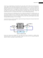
Both ideas allow different volume and user sound settings if they are applied in the preamp before the loudness
compensation. Change in volume or sound after loudness compensation will give rise to wrong compensation of the
playback signal if no corrections for these changes are added in the loudness compensation. The loudness
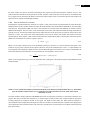
compensation shall be connected directly to the power amp for correct behavior. See Figure 6.3 for intended
implementation of the loudness compensation system in a car audio system.
FIGURE 6.3 - IMPLEMENTATION OF THE LOUDNESS COMPENSATION SYSTEM IN A CAR AUDIO SYSTEM.
The chosen solution is idea 2 because we believe we can create better noise estimations using this solution. Idea 1
needs a lot of parameters to perfectly estimate the noise and even though we maybe not are able to implement idea2
perfectly we believe idea2 still estimates better than idea1. Especially when parameters like road type changes, idea1
will have troubles. We have not investigated how much the noise is actually changing due to change of the hard
measureable parameters. It’s only based on our own experience.
27
Implementation
6.2 NOISE EXTRACTION
The idea behind the noise separation algorithm is simple: compare the recording in one position with the estimated
sound of the playback signal (which would be the program material convolved with the transfer function) in that
position. The difference of levels between the recording and the estimation should be given by the presence of noise
in the recording position. Therefore, the levels in the recorded position should always be higher than the estimated
levels. Of course, this difference can have other sources like: measurement noise (both on-line measurement and
transfer function measurement) or floating-point operations error, but we expect these not to dramatically affect a dB
of an RMS value. Thus, the comparison will be done in each of the 1-octave band (by comparing SPL value), thus both
the recording and the estimation of the playback signal should be transformed to Pascals. Naturally, the comparison
will be done by slicing the signal into smaller intervals. A block diagram of the noise extraction is depicted in Figure
6.4:
Octave Band Filters
Recorded signal [Pa]
Raw signal
Transfer function from
raw signal to recording
Position [Pa]
(time convolution)
Recorded
levels dB SPL
(rec position)
Extract
(Estimate)
Noise
Octave Band
Filters
Noise
levels dB SPL
(rec position)
Raw signal
levels dB SPL
(rec position)
FIGURE 6.4 - NOISE ESTIMATION BLOCK DIAGRAM
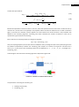
6.2.1 TESTING FOR RELIABILITY
To trust the method described above, we needed to test that the simulation of the program material was close
enough to a recording under the same conditions. Thus, we compared the simulation of the program material in the
front position of the microphone with the recording of the same playback signal played and recorded inside the car in
the same position with no engine running. The comparison was done each second (the slice length was 44100 samples
long) and the signals were adjusted as mentioned in 5.5 Car transfer functions. The signals were firstly analyzed
without the subtraction of the noise floor RMS value in the transfer function gain – a gain of 18.75 dB was computed.
The error graph was plotted for each second for each band (calculated as abs(Level_recording – Level_simulation):
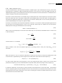
FIGURE 6.5 – ERROR BETWEEN SIMULATION AND RECORDING FOR EACH SLICE. SLICE SIZE = 1S.
28
Implementation
On the graph, the dotted black vertical lines represent separation of periods. Figure 6.6 depicts the average error for
each piece in the program material:
FIGURE 6.6 - AVERAGE ERROR PER PERIOD.
The exact values are depicted in DVD\Extra\Docs\Noise comparison.xlsx
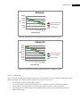
6.2.2 ANALYSIS OF DATA
In the silence period, the measurement picked only the noise floor while the simulation was constructed by
convolution with zeros. This accounts for the high average level in this period, Figure 6.6, and for the maximums in
Figure 6.5 when the periods change (fade-out + fade-in).
This explains the high levels of error for the 31 Hz band in many periods with little low frequency content (like Speech,
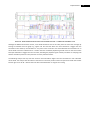
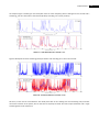
Opera or Classical periods) and it also accounts for some 63 Hz error. This is also depicted in Figure 6.7, Figure 6.8 and
Figure 6.9 where the red levels represent the recording’s levels and the blue one the simulated ones (analysis of
seconds 60 and 200 corresponding to speech period and classical period, respectively):
Speech period – second 60
Classical music – second 200
FIGURE 6.7 – COMPARISION BETWEEN SIMULATION AND RECORDING, FRONT MIC POSITION. LEVELS SIGNAL NOISE = RECORDING LEVELS. LEVEL
SIGNAL RAW = SIMULATED LEVELS.
29
Implementation
However, where the period contained more low frequencies, the estimation is close to the recorded playback
material:
Coldplay, Clocks – second 128
Trendermøller , snowflake – second 224
FIGURE 6.8 - COMPARISION BETWEEN SIMULATION AND RECORDING, FRONT MIC POSITION. LEVELS SIGNAL NOISE = RECORDING LEVELS. LEVEL
SIGNAL RAW = SIMULATED LEVELS.
By looking at the above graphs we can conclude that the simulation is close enough to the recording, a conclusion
enforced by the small error in the pink noise:
FIGURE 6.9 - COMPARISION BETWEEN SIMULATION AND RECORDING, FRONT MIC POSITION. LEVELS SIGNAL NOISE = RECORDING LEVELS. LEVEL
SIGNAL RAW = SIMULATED LEVELS. SECOND 11.
Interesting to mention in this comparison study is that the 31 Hz band is almost always higher in the recording than
the simulation. This is because of the shape of this filter (see 6.3.8 Octave band filter and equalizer) which could not
be fitted well inside the [IEC 61260 – 1995] specifications without a down-sampling: it picks not even playback signal
content from other bands, but also noise floor content from other bands. All the bar-graph analysis of the 1 second
slices in this comparison were put together with the program material (LeftChannel – the recording, RightChannel –
simulation; uncompressed sound; both converted from Pa to some DU in the same manner, both gained by 12 dB) in a
movie which can be found on the DVD\Video\Recording vs Simulation Front 12dB 1.0S slice.wmv. The process was
repeated without the delay adjustment mentioned in 5.5 Car transfer functions and the average errors values did not
change (expected for such a small delay given the slice length: about 200 samples compared to 44100 samples).
It should also be mentioned that the recorded signal should always be higher (or equal) to the simulation because of
the noise floor. In the presented graphs the analysis was done without the subtraction of the noise floor, that is why
the blue bars are usually higher.
30
Implementation
6.2.3 DECREASING SLICE SIZE
The slice size has been decreased to see how the simulation is working for smaller slices – different results are
expected due to dynamic differences in periods which would pick up the noise floor in-between the playback signal
content (the numbers will be seen in error graphs). Different slice size error graphs will be presented:
FIGURE 6.10 – ERROR BETWEEN SIMULATION AND RECORDING FOR EACH SLICE. SLICE SIZE = 0.5S. FRAME PER SECOND (FPS) = 2.
By analyzing individual bar frames, we can see that the small slices captures more music’s dynamics and thus the
simulation goes below the noise floor at each peak in the graph (graph depicting a 0.1 second slice of speech):
FIGURE 6.11 – BAR FRAME OF LEVELS OF SIMULATION AND RECORDING FOR SECOND 708 OF PROGRAM MATERIAL. LEVELS SIGNAL NOISE =
RECORDING LEVELS. LEVEL SIGNAL RAW = SIMULATED LEVELS.
A video was made with all the bar analysis for slice size = 0.1 s (see DVD\Video\Recording vs Simulation Front 12dB
0.1S slice.wmv).
31
Implementation
6.2.4 NOISE EXTRACTION
Based on the measurements SPL value (playback signal + noise – noted
) and the estimated sound in SPL for each
octave band (playback material– noted ) the noise (noise– noted ) in each octave band can be estimated:
(6.1)
{
Thus, an estimation of the noise in each band (RMS value for a certain slice):
(
)
(6.2)
The value
was set to 0 if
– in case of estimation errors. The estimation was first tested on the
program material for the front microphone position when engine was not running. The estimation should approach
the noise floor in all periods.
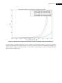
Figure 6.12 depicts the noise estimation for each slice (1 slice = 1 second) – the second period represents the noise
floor and the noise estimation should approach the values within that period:
FIGURE 6.12 – NOISE ESTIMATION FOR EACH SLICE IN OCTAVE BANDS. SLICE SIZE = 1S.
As can be seen in Figure 6.12, except maybe the 31 Hz band, the estimation does not approach the noise floor, in
many bands the difference being as big as 40dB. Some uncertainties may reside in the transfer function gain (in 5.5
Car transfer functions) and this could be a cause for this differences. By increasing the gain of the transfer function by
1.5 dB, we had the result in Figure 6.13:
32
Implementation
FIGURE 6.13 - NOISE ESTIMATION FOR EACH SLICE IN OCTAVE BANDS. SLICE SIZE = 1S. SIMULATION IS GAINED BY 1.5dB
Although the differences become smaller, some band estimations are too far away from the noise floor average. By
looking at individual slice bar graph e.g. Figure 6.11 we saw that when the noise estimation is bigger than the
simulation of the material, the estimation is very close to the noise floor. We concluded that the estimation for an
octave band cannot be trusted when it is smaller than the simulated playback signal SPL value for the same octave
band (the estimation is bigger than the real-value, following the playback signal content) and went on analyzing how
well the estimation performs in the presence of a more powerful masker.
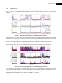
The following analysis will only take into account noise estimations higher than the simulation for each individual
octave band. The analysis was done with 1 second slice in the front position of the microphone and with the transfer
function gain of
– without the noise floor subtracted when no engine was running.
33
Implementation
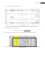
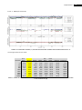
6.2.4.1 0 K M / H RECORDING – ENGINE RUNNING
FIGURE 6.14 – ESTIMATION OF THE NOISE (6.2) FOR EACH SLICE ONLY WHEN IT IS HIGHER THAN THE SIMULATION.SLICE SIZE = 1S.
The average values for each band, calculated as:
(
[ ]
where only the estimations
Band[Hz]
31
63
125
250
500
1000
2000
4000
8000
16000
)
Pink
Noise
64.22
0
0
0
0
0
0
0
0
40.92
Silence
66.75
58.69
56.14
50.07
41.92
30.83
29.31
31.66
34.46
36.92
[ ]
∑
(6.3)
[ ] were taken into account(1s slice):
Speech
65.74
57.86
0
0
0
0
47.9
32.36
36.21
37.23
Opera
66.17
57.01
52.92
46.25
0
0
53.98
29.08
32.62
36.63
Pop
Rock
65.62
57.31
53.6
48.17
40.09
26.83
42.78
31.52
34.02
36.7
Hard
Rock
65.94
56.42
55.06
49.24
41.63
30.66
29.19
31.5
34.46
37.49
Classical
66.57
57.19
54.66
46.97
0
0
39.74
29.06
32.87
36.75
Electronic
68.62
58.73
55.78
51.1
44.12
32.14
30.33
29.75
33.36
36.52
TABLE 6.1 – AVARAGE OF THE ESTIMATION OF THE NOISE (6.2) FOR EACH PERIOD ONLY WHEN IT IS HIGHER THAN THE SIMULATION.SLICE SIZE =
1S. THE VALUES ARE SPL [dB].
34
Implementation
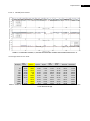
6.2.4.2 50 K M / H RECORDING
FIGURE 6.15 - ESTIMATION OF THE NOISE (6.2) FOR EACH SLICE ONLY WHEN IT IS HIGHER THAN THE SIMULATION.SLICE SIZE = 1S.
The average values for each band:
Band[Hz]
31
63
125
250
500
1000
2000
4000
8000
16000
Pink
Noise
84.53
75.62
66.09
63.46
57.47
54.32
49.12
0
46.87
41.43
Silence
82.61
75.19
67.1
64.68
59.68
48.9
39.13
32.77
34.11
36.52
Speech
82.12
76.37
65.23
62.34
56.98
46.82
37.5
29.42
38.48
36.11
Opera
83.81
78.46
69.54
64.17
57.56
48.68
49.76
31.65
32.93
36.21
Pop
Rock
85.91
76.89
70.69
65.76
61.84
58.58
46.83
46.74
36.74
36.51
Hard
Rock
84.53
73.92
66.96
64.99
57.29
51.05
43.08
37.14
39.4
36.88
Classical
85.61
75.72
67.01
65.55
58.33
50.46
44.59
35.07
33.39
36.36
Electronic
84.76
74.12
66.09
61.78
57.18
49.65
41.26
37.85
36.01
36
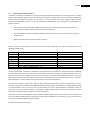
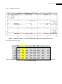
TABLE 6.2 - AVARAGE OF THE ESTIMATION OF THE NOISE (6.2) FOR EACH PERIOD ONLY WHEN IT IS HIGHER THAN THE SIMULATION.SLICE SIZE =
1S. THE VALUES ARE SPL [dB].
35
Implementation
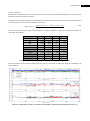
6.2.4.3 80 K M / H RECORDING
FIGURE 6.16 - ESTIMATION OF THE NOISE (6.2) FOR EACH SLICE ONLY WHEN IT IS HIGHER THAN THE SIMULATION.SLICE SIZE = 1S.
The average values for each band:
Band[Hz]
31
63
125
250
500
1000
2000
4000
8000
16000
Pink
Noise
81.19
73.66
67.29
66.42
57.5
53.99
0
0
0
41.63
Silence
81.28
75.34
70.66
70.06
61.31
55.55
45.95
37.59
34.69
36.95
Speech
82.33
76.8
69.42
67.4
58.92
53.75
44.79
35.86
38.73
36.98
Opera
81.44
74.25
69.79
65.9
58.34
52.6
51.55
35.04
34.62
37.06
Pop
Rock
82.63
75.47
69.37
66.53
60.18
53.44
46.86
35.48
34.65
36.7
Hard
Rock
83.75
75.27
68.47
65.62
59.32
54.02
45.63
37.35
34.59
37.95
Classical
85.52
78.44
69.56
67.15
61.27
54.88
47.97
36.16
34
36.78
Electronic
84.66
77.3
69.63
65.84
60.1
53.98
43.89
35.45
34.17
36.58
TABLE 6.3 - AVARAGE OF THE ESTIMATION OF THE NOISE (6.2) FOR EACH PERIOD ONLY WHEN IT IS HIGHER THAN THE SIMULATION.SLICE SIZE =
1S. THE VALUES ARE SPL [dB].
36
Implementation
6.2.4.4 110 K M / H RECORDING
FIGURE 6.17 - ESTIMATION OF THE NOISE (6.2) FOR EACH SLICE ONLY WHEN IT IS HIGHER THAN THE SIMULATION.SLICE SIZE = 1S.
The average values for each band:
Band[Hz]
31
63
125
250
500
1000
2000
4000
8000
16000
Pink
Noise
85.92
79.02
74.44
70.09
63.89
59.72
49.83
0
0
39.68
Silence
86.12
79.91
75.71
71.8
66
62.03
52.95
45.74
36.46
37.06
Speech
86.43
79.66
74.73
69.28
63.47
61.08
51.27
42.54
35.58
36.5
Opera
86.14
79.45
75.3
70.37
63.72
59.7
53.03
43.22
34.76
36.83
Pop
Rock
85.57
77.07
72.09
68.29
62.37
59.1
50.64
44.37
36.58
36.65
Hard
Rock
84.44
77.15
71.95
68.23
62.85
59.71
51.64
42.7
43.93
37.12
Classical
85.21
79.15
74.88
70.35
64.23
60.14
51.6
44.15
35.12
36.88
Electronic
85.96
77.29
71.73
68.69
63.23
59.69
51.28
43.47
36.44
36.45
TABLE 6.4 - AVARAGE OF THE ESTIMATION OF THE NOISE (6.2) FOR EACH PERIOD ONLY WHEN IT IS HIGHER THAN THE SIMULATION.SLICE SIZE =
1S. THE VALUES ARE SPL [dB].
37
Implementation
6.2.4.5 R ESULTS
We define the “velocity noise floor” as the SPL values for each octave band calculated during the silence period of the
playback material at constant car velocity.
The results show that the estimation is consistent with the velocity noise floor in the second period and the deviations
from the velocity noise floor were calculated for each band:
∑|
|
(6.4)
For all velocities Figure 6.14 to Figure 6.17 and Table 6.1 to Table 6.4(engine running) the averages were found for 1s
slice length. See Table 6.5.
Band [Hz] \ Velocity
50 Km/h
80 Km/h
110 Km/h
31
0 Km/h
2.53
3.3
4.24
1.68
63
2.27
3.27
3.1
2.84
125
3.22
3.59
3.37
3.98
250
3.82
2.9
4.44
3.57
500
2.2
2.7
3.81
3.63
1000
4
9.68
2.95
2.93
2000
13.47
10.63
5.6
3.12
4000
2.6
13.97
2.55
3.2
8000
1.84
12.76
4.04
7.47
16000
4
4.91
4.68
2.62
TABLE 6.5 – AVARAGE ERROR OF THE NOISE ESTIMATION. SLICE LENGTH = 1S. THE VLAUES ARE IN SPL.
The same comparison was done by lowering the slice size to 0.1 seconds. An estimation graph is presented for 50
Km/h recording:
FIGURE 6.18 - ESTIMATION OF THE NOISE (6.2) FOR EACH SLICE ONLY WHEN IT IS HIGHER THAN THE SIMULATION.SLICE SIZE = 0.1S.
38
Implementation
In this recording, the highest peaks in the low frequencies’ estimation (31 & 63 Hz) represent movement of the
microphone which will add to the average error. Additionally, because the recording was done twice, the program
material recorded at 50Km/h was put together manually from two individual recordings and because of this there is a
delay between the recording and the simulation – can be clearly heard since from Coldplay – Clocks period. An
animation was built with the simulated program material, recorded program material and estimated velocity noise
floor for front microphone position, 50 Km/h but no gain added to the playback – see DVD\Video\Noise Floor
Estimation 50 Km 0dB 0.1S slice.wmv). This delay will account for some high frequencies differences in this particular
velocity. For graphs for other velocities, see DVD\Extra\Docs\Noise comparison.xlsx.
The average error was computed for 0.1 time slice:
Band [Hz] \ Velocity
50 Km/h
80 Km/h
110 Km/h
31
0 Km/h
2.61
2.18
3.68
2.38
63
2.33
2.96
2.77
3.23
125
5.24
3.88
3.08
3.64
250
3.72
2.28
3.97
3.09
500
3.61
3.32
3.47
3.08
1000
21.32
7.48
1.79
2.91
2000
23.91
11.6
4.89
2.86
4000
3.99
19.89
5.41
2.39
8000
2.27
12.22
6.55
5.92
16000
4
4.89
4.66
2.58
TABLE 6.6 - AVARAGE ERROR OF THE NOISE ESTIMATION. SLICE LENGTH = 0.1S. THE VLAUES ARE IN SPL.
As can be seen, the average error drops for smaller time slicing – expected behavior since the algorithm is ‘dip
listening’ the noise within small pauses in the program material. Taking into account the noise distribution (see 5.4
Noise in the car) which is concentrated mostly in the lower frequencies and also the error of the estimation, the
estimation seems reasonable enough.
6.2.5 MICROPHONE POSITION FOR NOISE ESTIMATION
One recording position should be chosen. Since the on-line recording will be used solely for noise estimation, the
positioning of the microphone should best estimate the noise in the car (as close as possible to velocity noise floor
around the listener’s head) and should be robust enough to playback material and car velocity.
It should be noted that only the noise estimations (given in SPL for each band) greater than the simulation in recording
position were taken into account because of poor estimation when masking effect due to noise is not estimated (see
5.4 Noise in the car)
The chosen time slice length for the analysis was 0.1 seconds because the estimation improves with a smaller time
slice and the errors in estimation when playback signal levels are higher than the noise estimation is lower (see 5.4
Noise in the car).
39
Implementation
6.2.5.1 C OMPARISON OF N OISE ESTIMATIONS
The comparison will be done for different positions and different velocities of the car. Data extraction values will be
given in SPL.
For a given recording at a specific velocity, the noise estimated for each octave band in each slice is averaged for each
period by averaging across all slices:
(6.5)
∑
|
[ ]
Where K represents the slices contained in a period and Period is one Part of the test signal (generally one song,
silence, or pink noise) expressed in seconds.
This way, the average in the second period should be close enough the velocity noise floor found in 5.4 Noise in the
car, which is computed taking in account the RMS value of an entire period and here the noise floor is done by
averaging RMS values of smaller slices, concretely 0.1 seconds as it is mentioned before.
Noise floor values found for one octave bands and different velocities can be found on DVD\Extra\Docs\Noise
comparison.xlsx. This velocity noise floor will be noted as
, where i represents the octave band and the
velocity is the car velocity in Km/h.
6.2.5.2 NF I , V EL OCITY D EVIATON
We now want to study the deviation from
and
for each recording position. For this, the difference between
was computed for a fixed velocity:
(
)
In order to work with less amount of data, an average across periods (of course, except the
(6.6)
) was computed
for each band i at a fixed velocity:
(6.7)
∑
An example for such a computation (0.1 s slice, velocity = 80 Km/h, recording position at ear level –front of listener) is
shown in Table 6.7 and Table 6.8:
Period
Band
31
Pink
Noise
83.14
16000
48.86
Speech
Opera
Hard
Rock
82.69
Classical
Electronic
83.28
Pop
Rock
83.53
83.09
83.13
37.26
38.52
82.98
81.18
36.47
38.06
40.95
36.64
36.9
TABLE 6.7 - SPL FOR EACH PERIOD. TIME SLICE 0.1S, VELOCITY 80 KM/H.
The Deviation is then:
Band(i)
31
0.05
0.04
0.19
0.44
0.4
0.11
1.91
0.45
16000
11.6
1.26
0.79
0.8
3.69
0.62
0.36
2.73
TABLE 6.8 – ERROR AND AVERAGE DEVIATION SPL FOR EACH PERIOD. TIME SLICE 0.1S, VELOCITY 80 KM/H.
40
Implementation
All data (
) was then collected for three microphone positions, Front, Ear Level, Back. For all
values collected (also for 1 second slice), see the project’s DVD\Extra\Docs\ Noise comparison.xlsx.
For the three microphone positions, the average errors for each band and velocity
Average Noise Estimation Error 0.1s Slice - 50 Km/h
14,00
Average error [dB]
12,00
10,00
8,00
6,00
Back Position
4,00
Ear level Position
2,00
Front Position
0,00
31
Hz
63 125 250 0.5 1
2
4
8 16
Hz Hz Hz kHz kHz kHz kHz kHz kHz
Frequency
FIGURE 6.19 - AVERAGE NOISE ESTIMATION ERROR 0.1S SLICE - 50 KM/H.
Average Noise Estimation Error 0.1s Slice - 80 Km/h
8,00
Average error [dB]
7,00
6,00
5,00
4,00
Back Position
3,00
Ear level Position
2,00
Front Position
1,00
0,00
31
Hz
63 125 250 0.5 1
2
4
8 16
Hz Hz Hz kHz kHz kHz kHz kHz kHz
Frequency
Average error [dB]
FIGURE 6.20 - AVERAGE NOISE ESTIMATION ERROR 0.1S SLICE - 80 KM/H.
8,00
7,00
6,00
5,00
4,00
3,00
2,00
1,00
0,00
Average Noise Estimation Error 0.1s Slice - 110
Km/h
Back Position
Ear level Position
Front Position
31 Hz63 Hz 125 250 0.5 1 kHz 2 kHz 4 kHz 8 kHz 16
Hz Hz kHz
kHz
Frequency
FIGURE 6.21 - AVERAGE NOISE ESTIMATION ERROR 0.1S SLICE - 110 KM/H.
are plotted:
41
Implementation
6.2.5.3 F IRST C OMPARISON
The back of listener head has the biggest deviation from the velocity noise floor. The lowest error in low frequencies is
achieved by the ear level listening position except for the velocity of 50 Km/h. The front position shows relatively
small deviations from the velocity noise floor and outperforms other microphone positions at the velocity of 50 Km/h.
6.2.5.4 S ECOND C OMPARISON
Second comparison was done to see how close the estimation for each band is to the velocity noise floor, as
calculated in 5.4 Noise in the car, where for each band, the RMS value of the entire silence period was computed.
Again, additional averaging needs to be done in order for the comparison to be done. First of all, an average across
periods needed to be done for each band (the silence period was ignored for a better comparison) – at constant
velocity:
(6.8)
∑
From the graphs in 5.4 Noise in the car, we can see that the noise floor in the back position always exceeds the noise
floor at ear level, sometimes as high as 10 dBs more. Also, taking into account the deviation in the first comparison for
this microphone positioning, the back position recordings were discarded for this comparison.
Secondly, the velocity noise floor was calculated for four different positions (three because we leave out the back
microphone position). The graphs in 5.4 Noise in the car, show that the noise floor in the remaining three positions
are close enough but an average of these positions was done to get an ‘overall’ velocity noise floor in the car:
(6.9)
∑
The values for the averages are found on the project’s DVD\Extra\Docs\Noise comparison.xlsx & Noise Floor
deviation.xlsx.
The results are depicted in Figure 6.22, Figure 6.23 and Figure 6.24:
100,00
90,00
80,00
70,00
60,00
50,00
40,00
30,00
20,00
10,00
0,00
Velocity Noise
Floor
Ear Level Position
Front Position
31
63
125
250
500
1000
2000
4000
8000
16000
dB
50 Km/h
Frequency [Hz]
FIGURE 6.22 - ESTIMATION VS AVG VELOCITY NOISE FLOOR IN THE CAR - 50 KM/H (0.1 S SLICE).
42
Implementation
80 Km/h
100,00
dB
80,00
60,00
40,00
Velocity Noise Floor
20,00
Ear Level Position
Front Position
31
63
125
250
500
1000
2000
4000
8000
16000
0,00
Frequency [Hz]
FIGURE 6.23 - ESTIMATION VS AVG VELOCITY NOISE FLOOR IN THE CAR - 80 KM/H (0.1 S SLICE).
90,0
80,0
70,0
60,0
50,0
40,0
30,0
20,0
10,0
0,0
Velocity Noise Floor
Ear Level Position
Front Position
31
63
125
250
500
1000
2000
4000
8000
16000
dB
110 Km/h
Frequency [Hz]
FIGURE 6.24 - ESTIMATION VS AVG VELOCITY NOISE FLOOR IN THE CAR - 110 KM/H (0.1 S SLICE).
6.2.5.5 C ONCLUSIONS
We can conclude that the best microphone position for noise extraction is the front position. Regarding the front
position and based on the previous section comparison conclusion we can say that:




The estimation can also be used for other listeners.
The transfer function measured at this position is less susceptible to variance from listener movement.
The noise floor in ear level position is very close to the velocity noise floor in the front position.
The averaging done in equation (6.9) is not very different to the value found at ear level (see section 5.4.4
Results and analyzing)
43
Implementation
6.3 LOUDNESS AND MASKING COMPENSATION
From section 5.6 Loudness, none of the analized loudness models and calculations seems to fit perfectly to our
problem. The loudness models by [Skovenborg, 2004] estimates the loudness of music and speech well but don’t take
into account noise. And the loudness calulation from [Lochner & Burger, 1961] which calculates the loudness of a
signal present in noise, have some disadvantages. The calculation is only confirmed valid in the bandwidth 200-8000Hz
and with pure tones. Our playback signal has a wider bandwidth and contains complex tones. Temporal, forward and
backward masking are also not taken into account in this calculation. However the loudness function by [Lochner &
Burger, 1961] is the only approach we have found for calculation of loudness of a signal present in noise. Our loudness
compensation system, Figure 6.25, is therefore formed around this function and used in the gain calculations block.
FIGURE 6.25 - BLOCK DIAGRAM OF THE LOUDNESS COMPENSATION. SIGNAL IS PLAYBACK SIGNAL
The main idea in the loudness compensation system is to compare the perceived loudness of the playback signal in a
reference condition (signal threshold block) with the perceived loudness of the playback signal in the noisy conditions
(noise threshold block). With help from this comparison we want to calculate a gain (gain calculation block) which can
be applied to the playback signal in noise condition (octave band equalizer) thus the loudness in the reference
condition is equal to loudness in the noisy condition. It is somehow a signal to masker ratio comparison. To avoid too
rapidly changing in the gain, a gain smoothing block is applied. The input signal is a slice with a chosen length and for
every slice all calculations are repeated. This gives an iteration time and averaging of the input signals depends on the
slice length. The transfer function blocks are applied because the calculations in the threshold level blocks are based
on signal levels at cochlea at listener position in the car.
From 5.4 Noise in the car, we know that the noise is louder in the lower frequencies than the higher frequencies. The
lower frequencies in the signal will therefore more often be masked than the higher frequencies. Due to this we have
decided to divide the loudness calculation and compensation into octave bands. This gives us the possibility to only
change the gain in the needed bands. The function by [Lochner & Burger, 1961] is also based on octave band noise
and fits therefore well our decision.
The total loudness compensation can then be described as a multiband loudness model based on [Lochner & Burger,
1961] which output a loudness compensated signal in slices. The model only takes simultaneously masking into
account and averaging the signal due to slicing. When phenomena’s like forward or backward masking is present, due
to e.g. passing car or highly dynamic signal, the system is not expected to compensate correctly. Compression effects
or pumping are expected when a signal is played at low levels but depends on the length of the signal slicing (iteration
time), gain smoothing and the dynamics in the signal.
44
Implementation
6.3.1 SIGNAL TO DIFFUSE FIELD TRANSFER FUNCTION
The signal to diffuse field transfer function is the measured car transfer function for microphone position, front. 9.1.2
Car transfer function measurements.
6.3.2 DIFFUSE FIELD TO COCHLEA TRANSFER FUNCTION
6.3.2.1 D IFFUSE FIELD TO EARDRUM TRANSFER FUNCTION
This chapter is based on the American Standard [ANSI S3.4-2005]. In this paper we can find two kinds of transfer
functions, depending on the characteristics of the sound field.


Free field: No reflections, with a frontal incidence of the sound source.
Diffuse field: Reflections and refractions are present. Usually used for rooms with low-normal absorption,
enclosures, etc.
A diffuse field seems to be the most suitable scenario in a car cabin. The American standard [ANSI S3.4-2005],
describes this influence as the difference of the sound pressure level in the eardrum, and the sound pressure level
measured in the diffuse field in the absence of a listener.
A transfer function (H1) in third octave bands in the audible frequency range (20 Hz-20000 Hz) is given, where the
values correspond to the difference mentioned before. Therefore if a compensation due to this factor is wanted, a
sum of this values in SPL should be applied to the spectrum in SPL as well.
(
(
)
)
(
(
)
)
(
)
(6.10)
(
)
(6.11)
In order to have a better resolution an interpolation is done between the data points given in this curve.
Since in this project this transfer function will be computed in time, a signal in time domain with the characteristic
frequency spectrum of the compensation curve should be computed, in order to convolute this signal with the input
that needs to be compensated. The signals which we are going to apply the compensation are expressed in pressure
[Pa], therefore a gain function corresponding to the compensation curve given in dB in the [ANSI S3.4-2005], is
computed in pressure [Pa]. The result in frequency domain will be a multiplication of the characteristic spectrum of
the gain curve and the spectrum of the signal in which the compensation want to be applied. Thereby a SPL value of 0
dB corresponds to gain of 1. The formula to work out the gain is shown in (6.12):
(
)
(6.12)
Where SPL: is the amount of dB that we want to increase. The resolution in the interpolated curve depends directly on
the desired number of samples of the impulse signal returned by the function. A plot of the transfer function from
diffuse field to Eardrum given in SPL in the [ANSI S3.4-2005] with cubic interpolation is shown in Figure 6.26.
45
Implementation
FIGURE 6.26 – DIFUSE FIELD TO EARDRUM TRANSFER FUNCTION. SETS OF THREE ADJACENT VALUES IS SHOWED IN THE RED BOXES.
The curve given in the [ANSI S3.4-2005] standard has been expanded from 0 to 22050 Hz. As no information in 0-20Hz
and 20000-22050Hz is known, the gain for this frequencies has been fixed to 1 (this means no change in the output for
this frequencies). In addition, once the convolution is done, a spectrum analysis from 20-20000 Hz will be the most
suitable frequency range for study.
6.3.2.2 E ARDRUM TO COCHLEA TRANSFER FUNCTION
The aim of this section is to get the filter to apply to the input signal to simulate the behavior of the middle ear,
concretely from eardrum to the cochlea. This section is based in the standard [ANSI S3.4-2005]. The transfer function
to take in account from the eardrum to the cochlea is defined in the standard [ANSI S3.4-2005] as the SPL in the
cochlea in relation with the SPL in the eardrum. This is:
(
)
(
)
(
)
(6.13)
The transfer function is given in SPL in frequency. The frequency range corresponds to the audible frequency range,
this is 20Hz-20KHz, expressed in third octaves. According to [ANSI S3.4-2005], an interpolation of this curve based on a
second order polynomial function which fits to sets of three adjacent data points in a linear frequency scale is defined.
FIGURE 6.27 – EARDRUM TO COCHLEA TRANSFER FUNCTION. SETS OF THREE ADJACENT VALUES IS SHOWED IN THE RED BOXES.
46
Implementation
It is worth to mention that the interpolation is made in a linear frequency scale, but the Figure 6.27 is presented in a
logarithmic scale for viewing purposes.
The function used for the interpolation in python has been “scipy.interpolation.interp1d” which allows to make an
approximation of a function in 1 dimension in the form y=f(x).
The kind of interpolation used has been ‘cubic’ which is actually a third order approximation of the curve. This kind of
interpolation has been decided for its better result than a linear interpolation.
As the transfer function to the eardrum, this transfer function is going to be applied to the input signal in time domain,
so a filter should be derived from the characteristic spectrum. The input signal is expressed in Pascals, therefore the
spectrum shown in Figure 6.27 should be transformed into gain for being applied to the input. The gain is worked out
as in (6.12).
6.3.2.3 D IFFUSE FIELD TO COCHLEA TRANSFER FUNCTION
Since two different transfer functions have to be applied to the input signal, first the transfer function to take in
account from diffuse field to the eardrum, and then the middle ear transfer function with no intermediate
computations between them, a combined transfer function has been decided to be applied for computational
efficiency. Therefore just one convolution operation will be computed instead of two. As the transfer functions shown
in the sections 6.3.2.1 Diffuse field to eardrum transfer function and 6.3.2.2 Eardrum to cochlea transfer function are
expressed with the same concept of SPL difference between two points, the combined transfer function can be
expressed with the same concept, where the values of the transfer function is the addition of both.
FIGURE 6.28 - COMBINED TRANSFER FUNCTION.
Where:
(6.14)
(6.15)
(6.16)
(6.17)
The new values of H are computed by addition of H1 and H2 values given in SPL. The new values are computed for the
frequency range given in the [ANSI S3.4-2005]. These new values in SPL are shown in Figure 6.29:
47
Implementation
FIGURE 6.29 - COMBINED TRANSFER FUNCTION SPL.
Then the values in SPL of the combined transfer function are converted to gain using (6.12) in order to be able to
apply it to the input signal. See Figure 6.30.
FIGURE 6.30 – DIFFUSE FIELD TO COCHLEA TRANSFER FUNCTION IN GAINS.
6.3.2.4 I MPLEMENTATION OF THE C OMBINED T RANSFER F UNCTION TO THE INPUT SIGNAL
As it is mentioned in the section before, the combined transfer function is converted into gain for its application to the
input signal. In the project, this implementation has been applied into two different signal input formats. Two
different functions have been made in python for this purpose. Both can be found module called DVD\Codes\Python
codes\Head_and_Torso_Transfer_Function\HHTF_Project.py. HTTF is a function to compute the filter regarding to the
combined transfer function in time domain.
DVD\Codes\Python_codes\Head_and_Torso_Transfer_Function\HHTF_Project.py.HTTF_Octave_bands.py is the
function made for computing the transfer function in frequency domain (octave bands). It should be noted that all
fourier transforms applied to different signals for the combined transfer function analysis have been computed with
the same amount of points (NFFT) as the length of the signals for which it has been applied.
48
Implementation
6.3.2.5 I NPUT SIGNAL -T IME D OMAIN
For the implementation of the combined transfer function, a filter in time domain is built from the information in the
frequency domain. Some parameters of the filter should be defined. These parameters were chosen after some tests
which will be explained following. The parameters are:




Frequency Response: It is clear that the frequency response of the filter should be the most close to the
theoretical worked out (Gain).
Delay: It’s defined as the number of samples before the main peak of the filter.
Phase Response: No information about the phase in the standard [ANSI S3.4-2005] is mentioned. No
influence of phase for loudness compensation is taken into account, therefore it has not been taken in
account for the filter design.
Duration of the filter: It’s basically the length of the signal in time. The number of samples is a trade-off
between desired frequency response and the time needed for convolution computation
6.3.2.5.1 F REQUENCY R ESPONSE (G AIN )
The frequency response should be the gain computed to be applied to the input signal for this section. The resolution
of this gain depends on the length of the impulse response desired (samples), so an interpolation as it is explained in
section 6.3.2.1 Diffuse field to eardrum transfer function, will be computed. The amount of points in the function gain
interpolated will be the same as the desired samples. Once the frequency response is obtained, an entire model
spectrum is built. This spectrum will include the frequency range [0-22050 Hz) and the negative part of this spectrum
is obtained computing the conjugate of the positive part. Therefore the number of points obtained for the entire
spectrum is the double of the number of samples introduced in the function HTTF() inside DVD\Codes\Python
codes\Head_and_Torso_Transfer_Function\HHTF_Project.py minus one sample due to the repetition of the sample
corresponding to 0 Hz. As no information about the response of this frequency range is available, it is decided to have
the same response that 20 Hz. It is worth to mention that this approximation has no influence in the filtered signal,
since the audible range is above 20 Hz.
Once the desired frequency response is built an inverse fourier transform is made (numpy.fft.ifft function is used for
that purpose). The number of samples after the computation will be the same as the NFFT included in the desired
spectrum, so this length in samples will be controlled by the amount of samples in the interpolation of the desired
spectrum as it is mentioned before. Once the IFFT is computed, the output is circularly shifted (rolled) by half of its
length in order to get an impulse response which contains the desired frequency response information, and then the
amount of undesired samples are removed from the extremes of the symmetric impulse response. A FFT of the rolled
output is computed and compared with the desired frequency response is shown in Figure 6.31 and Figure 6.32:
FIGURE 6.31 - IMPULSE RESPONSE. 3000 SAMPLES.
49
Implementation
FIGURE 6.32 - FFT OF IMPULSE RESPONSE 3000 SAMPLES.
As can be seen in the figure Figure 6.32, the response in frequency of the impulse response is very close to the
theoretical gain. It is worth to clarify that Figure 6.32 shows the positive frequency range of the FFT due to the
logarithmic scale of the plot.
6.3.2.5.2 D ELAY
Once the impulse response is built, it is decided to include as less amount of delay as possible. Delay is considered the
samples before the main peak on the impulse response which is in the center of the impulse response respect to time.
The procedure to do so is:
First a window of time samples has to be fixed, then the maximum peak of the impulse response is moved to time
zero of the window. Once we have the impulse response in this position (0 delay), samples from the left part of the
impulse response or from the right can be taken in account. In other words we can choose the delay just taking a
number of samples before the main peak of the impulse response, and to maintain the desired number of samples we
can discard samples from the end of the impulse response. With this method, we can create a new impulse response
with a desired delay. Since information about frequency response of the impulse response is before the main peak, a
test was made in order to know the amount of samples before the main peak of the impulse response (delay) has to
be taken in account to have an acceptable frequency response.
FIGURE 6.33 - IMPULSE RESPONSE 2500 SAMPLES WITH NO DELAY.
50
Implementation
As can be seen when no delay is included in the impulse response, too much information about the behavior in
frequency is lost, and the frequency response is not acceptable for our purposes.
FIGURE 6.34 - IMPULSE RESPONSE 2500 SAMPLES WITH 250 SAMPLES OF DELAY.
In Figure 6.34, an impulse response of 2500 samples and 250 samples of delay is shown. As we can see the frequency
response is acceptable in all the frequency range that we are interested in. In this report, just two examples of the
different lengths and delays are shown, although more tests were done. A script for testing different lengths is
included in DVD\Codes\Python codes\_Analysis\Test_HTTF.py
6.3.2.5.3 P HASE R ESPONSE
Regarding phase response, there is no information about it in [ANSI S3.4-2005] standard. After studying the different
blocks, which the present project consists of, no phase information is taken in account for any of the mentioned
blocks, therefore the phase response has not been taken in account in the construction of the filter.
6.3.2.5.4 D URATION OF THE FILTER
The duration of the filter has been chosen taking in account different aspects. The frequency response should be
acceptable, and convolution computation time should be fast enough for an on-line loudness compensation system.
Considering all the aspects mentioned before, a 2500 samples with 250 samples of delay filter has been chosen for
use in the loudness compensation system
6.3.2.6 T EST OF THE C OMBINED T RANSFER F UNCTION
Once the main characteristics of the filter have been decided and the filter is built we can test the filter and check its
behavior in frequency domain. Two different tests have been done. First a convolution of the impulse response
computed with the function HTTF() and dirac delta is studied. Secondly, a high frequency resolution study of the
impulse response behavior is made. The tests are made in a python script DVD\Codes\Python
codes\_Analysis\Test_HTTF.py.
51
Implementation
A dirac delta is built for test the filter. As it is known a Dirac delta is defined in time as:
( )
{
(6.18)
Dirac delta has a flat response for the entire frequency domain and it is the identity element for convolution.
An impulse response (filter) is generated with a function called HTTF() created in python in which can be found in the
script DVD\Codes\Python codes\Head_and_Torso_Transfer_Function\HHTF_Project.py. The length of the filter is 3000
samples including a delay of 250 samples. The filter is convoluted with a Dirac delta mentioned before. A FFT is
applied to the result of the convolution in order to know the frequency response. As we know:
H(x)*δ(x)=H(x)
(6.19)
Therefore the expected frequency response of the convolution should be the gain computed in section 6.3.2.3 Diffuse
field to cochlea transfer function. The result of the convolution and its frequency response is shown in Figure 6.35. As
can be seen, the behavior of the filter in frequency fits with the desired gain.
FIGURE 6.35 - CONVOLUTION OF A FILTER OF 3000 SAMPLES INCLUIDING A DELAY OF 250 SAMPLES WITH A DIRAC DELTA. TIME AND
FREQUENCY DOMAIN.
6.3.2.7 H IGH F REQUENCY R ESOLUTION OF I MPULSE R ESPONSE
In order to study the behavior of the impulse response with high frequency resolution, a vector of zeros has been
appended to the output of the HTTF() function. The amount of zeros is nine times the length of the impulse response
computed. Then, a FFT with:
NFFT=length(Impulse Response + zeros_vector)
(6.20)
is computed. The result is compare with the theoretical desired impulse response behavior (Gain). A plot of the result
is shown in Figure 6.36. The length of the computed impulse response (output of HTTF function) has been 3000
samples including 250 samples of delay.
52
Implementation
FIGURE 6.36 - FFT OF THE COMPUTED COMBINED TRANSFER FUNCTION IMPULSE RESPONSE WITH NFFT 30000.
As can be seen from Figure 6.36 the behavior of the impulse response is acceptable for the purpose of the present
project.
6.3.2.8 I NPUT SIGNAL - FREQUENCY OCTAVE BANDS
In order to be able to compare the playback material with the measured one, there is a point in the chain where a
bank of filters applied to the input signal in time (playback signal), in order to get a signal representation in octave
bands. At the same time an octave band combined transfer function is needed. In [ANSI S3.4-2005] standard, values in
third octave bands are present. In order to get the correct values for octave bands two possibilities have been studied.

Values of center frequencies of octave bands in [ANSI S3.4-2005] standard. These are the values
corresponding to the center frequencies of each octave band that have been computed according to [IEC
61260] standard, taking from the values given in the [ANSI S3.4-2005].

Average of frequencies values contained in an octave band. These are the averages in SPL of the values in
third octaves bands given in the [ANSI S3.4-2005] standard.
In Figure 6.37 differences between these two options can be seen.
53
Implementation
FIGURE 6.37 – CENTER FFREQUENCY VALUES AGAINST AVARRAGE FREQUENCY VALUES OF THE COMBINED TRANSFER FUNCTION.
As it can be seen, the differences between them are very small, so the decision is not expected to have a big influence
in the behavior of the loudness compensation system.
As the octave band filters represents the rms value of the signal in an entire octave band frequency range, it seems
reasonable that the average influence of the frequency response within an octave band should be taken into account.
Thus, we decided to apply an average of the combined transfer function frequency response for each band.
54
Implementation
6.3.3 NOISE THRESHOLD LEVELS
The noise threshold level is the threshold level where a playback signal is just masked by the noise. E.g. If the noise
threshold level is calculated to 70dB, a playback signal present in this noise has to be at least 70dB to be heard. At
70dB the playback signal is just masked. Due to the use of octave bands the noise threshold level is calculated for each
of them. This gives in total 10 noise threshold levels.
Each of the noise threshold levels are calculated using an auditory filter with a center frequency for the chosen octave
band. This means that noise in all bands can affect the noise threshold level for the chosen band. The auditory filter is
calculated using [ANSI S3.4-2005] and for masking point of view the auditory filter can be mirrored upside down to
present PTC(Psychophysical tuning curves) [Moore, 2005].
First step is to calculate the filter shape which depends on the SPL. In our case this is both the playback signal SPL and
the noise SPL at the recording position in the car, the total SPL. Several steps are needed. First we calculate the
ERBN(equivalent rectangular bandwidth for normal hearing):
(
)
(6.21)
Where f is the center frequency for the chosen band. Next step is to calculate P51, P51at1KHz which are values used
in later calculations.
(6.22)
(6.23)
Then the value Plower is calculated
(
)
(6.24)
Where TotalSPL is the noise and playback signal SPL at recording position. Finally, the shape W(finput) can be
calculated:
(
)
(
|
|)
|
|
(6.25)
Where P is equal Plower if finput is less than f. Otherwise P is equal P51. Last step is to convert the auditory filter to dB
scale and mirror it (upside down), which will give us the auditory filter shape with the center frequency f:
(
)
( (
))
(6.26)
For every octave band (with center frequency ) the noise threshold level given by these on the chosen band
(centered on frequency ) is then calculated with the computed auditory filter
(having a center frequency ):
( )
(
( )
( ))
(6.27)
It should be noted that can be equal to which calculates the threshold level in the chosen band – the threshold
level for a playback signal to be just masked by the noise in the chosen band. The maximum value of these is the noise
threshold level for the chosen band which is the same as selecting the maximum masked threshold for the chosen
band from the PTC of all the other bands.
55
Implementation
Threshold shift is the level between noise SPL and the level where a signal is just masked by the noise within the same
band. We have chosen a fixed value of 18.5dB by studying the figures in [Moore, 2012]. The described calculations are
for one single band and they are therefore repeated 10 times in the software. Figure 6.38 and Figure 6.39 illustrates
different noise spectrums and the calculations for the noise threshold levels for the 1KHz band with different noise
spectrums.
FIGURE 6.38 - ILLUSTRATION OF THE NOISE THRESHOLD LEVEL CALCULATION FOR THE 1KHZ OCTAVE BAND USING AUDITORY FILTER. THE BARS
ARE NOISE IN OCTAVE BANDS. IN THIS CASE, THE NOISE THRESHOLD LEVEL IS AFFECTED BY THE NOISE IN THE 1KHZ OCTAVE BAND. ALL OTHER
NOISE BANDS ARE BELOW THE AUDITORY FILTER AND DO THEREFORE NOT AFFECTS THE NOISE THRESHOLD LEVEL.
FIGURE 6.39 - ILLUSTRATION OF THE NOISE THRESHOLD LEVEL CALCULATION FOR THE 1KHZ OCTAVE BAND USING AUDITORY FILTER. THE BARS
ARE NOISE IN OCTAVE BANDS. IN THIS CASE, THE NOISE THRESHOLD LEVEL IS AFFECTED BY THE NOISE IN THE 31HZ OCTAVE BAND. ALL OTHER
NOISE BANDS ARE BELOW THE AUDITORY FILTER (WHEN THRESHOLD SHIFT IS TAKEN INTO ACCOUNT) AND DO THEREFORE NOT AFFECTS THE
NOISE THRESHOLD LEVEL.
56
Implementation
6.3.4 SIGNAL THRESHOLD LEVEL
The signal threshold level is the level where the playback signal masks itself or is not hearable due to the hearing
threshold, therefore the maximum between the hearing threshold and the masking threshold level within the signal
itself is taken. The calculations for signal/hearing threshold level are almost equal to the noise threshold level
calculations. The difference is that the signal/hearing threshold doesn’t take into account the signal SPL in the octave
band where the signal threshold level is calculated. We are doing this to avoid that the chosen octave band masks
itself and only the other bands affect the signal threshold level. Figure 6.40 illustrates this. The signal threshold level
cannot be lower than the hearing threshold for the chosen band.
FIGURE 6.40 - ILLUSTRATION OF THE SIGNAL THRESHOLD LEVEL CALCULATION FOR THE 1KHZ OCTAVE BAND USING AUDITORY FILTER. THE BARS
ARE SIGNAL SPLS IN OCTAVE BANDS AND THE 1KHZ BAND, MARKED WITH GRAY, IS NOT TAKEN INTO ACCOUNT FOR THE CALCULATION OF THE
1KHZ SIGNAL THRESHOLD LEVEL. IN THIS CASE, THE SIGNAL THRESHOLD LEVEL IS THEREFORE ONLY AFFECTED BY THE SIGNAL IN THE 31HZ
OCTAVE BAND AND NOT THE 1KHZ BAND. ALL OTHER SIGNAL BANDS ARE BELOW THE AUDITORY FILTER (WHEN THRESHOLD SHIFT IS TAKEN
INTO ACCOUNT) AND DO THEREFORE NOT AFFECTS THE SIGNAL THRESHOLD LEVEL.
57
Implementation
6.3.5 HEARING THRESHOLD
According to [ISO 389-7], the hearing threshold is the level of a sound at which a person gives the 50% of correct
detection responses on repeated trials
One of the inputs for the signal threshold level block see Figure 6.25 is the threshold hearing of the human being at
each frequency band. Concretely, the audible frequency range is studied in octave band.
For this purpose the European standard [ISO 389-7] has been used as a reference for the threshold hearing levels. In
this document two different hearing thresholds are available depending on the sound field where it is applied. We
assume that the sound field in a car audio cabin is a diffuse field, that means that we expect that the reflections of the
sound will arrived from all directions.
The levels in one third octave band in SPL are shown in Figure 6.41.
FIGURE 6.41 - TRESHOLD HEARING. SPL (dB) THIRD OCTAVE VALUES.
This hearing threshold parameter is used in 6.3.4 Signal threshold level. This study is done in octave bands and in
order to get this octave band values the same procedure as in section 6.3.2.4 Implementation of the Combined
Transfer Function to the input signal, is done.
In order to increase the resolution of the curve for computing the average values for each center frequency, an
interpolation of the curve is made. This interpolation is made using the python function scipy.interpolate.interp1d in
linear scale. Once the interpolation is made, and average of the frequency values which are inside of the frequency
range determined by the octave band filters is made.
The average values used in the present project given in SPL:
Frequency (Hz)
SPL (dB) Average
31.5
59.77
63
37.67
125
22.17
250
11.4
500
3.9
Frequency (Hz)
SPL (dB) Aveage
1000
1.23
2000
-0.78
4000
-3.4
8000
6.73
16000
27.1
TABLE 6.9 - SPL (dB) AVERAGE VALUES FOR HEARING TRESHOLD.
58
Implementation
6.3.6 GAIN CALCULATIONS
The gain calculations are based on the loudness model by [Lochner & Burger, 1961] which are described in 5.6.2
Partial masking of loudness This model calculates the perceived loudness in sones for a signal in noise and because the
experiments by Lochner and Burger for this loudness model use octave band noise, the model fits well to our
solution/implementation. We are also using octave bands and a gain factor is calculated for each of them. In total 10
gain factors are calculated.
To calculate the gain we compare the perceived loudness for the playback signal in reference conditions (signal
threshold level) with the perceived loudness for the signal in noise conditions(noise threshold level).
The loudness in reference conditions is:
(
)
(6.28)
Where I is the playback signal intensity and Iref is the noise intensity threshold in reference condition. k and n are
constants described in 5.6.2 Partial masking of loudness
The loudness in noise conditions is:
(
)
(6.29)
Where I is the playback signal intensity and Inoise is the noise intensity threshold in noise condition (the estimated noise
level in each band).
We want the loudness for reference and noise condition to be equal and it is therefore necessary to multiply a gain
factor with the signal intensity in (6.29). The gain factor is multiplied with the playback signal intensity because we are
able to adjust the signal intensity in practice. (6.28)and (6.29) with the gain factor can then be combined.
(
)
((
)
)
(6.30)
Isolating the gain:
(
)
( (
))
(6.31)
The gain can now be calculated using signal intensity, reference threshold intensity and noise threshold intensity.
Finally the input intensities are converted to SPL using (6.32):
(
)
(6.32)
Where I is the intensity level and L is the SPL. (6.31) with (6.32) applied to all intensity levels is plotted in Figure 6.42.
59
Implementation
FIGURE 6.42 - GAIN WHEN NOISE THRESHOLD LEVELS ARE VARIED. THE SIGNAL AND REFERENCE THRESHOLD HAVE FIXED VALUES.
To avoid clipping or variable overflow, gain limits is applied in the developed software. The limits are especially
necessary at low signal levels or high noise levels. In these cases the gain calculation will calculate a large gain and
maybe introduce clipping or overflow if the gain is not limited. The minimum gain is limited to 1 because we don’t
want to damp the playback signal.
60
Implementation
6.3.7 GAIN SMOOTHING
After a simulation of the system – the program material and the recording at 50 Km/h (front microphone position) as
inputs – in slices of 1 second with the noise detection and gain blocks put together, the gains for each band were
analyzed:
FIGURE 6.43 - GAINS FOR EACH BAND FOR SLICE OF 1 SECOND (50 KM/H FRONT POSITION).
Important to mention in this simulation is that the system did not have any feedback (playback signal was not changed
from slice to slice, only the gains calculated for each slice), thus the gains should reflect a combination of the velocity
noise floor and periods’ dynamics. If this were done, a new recording would have been needed with the recorded
change into the playback signal. Also, the gain was capped to 15 as a maximum and to 0 as a minimum value.
Same analysis was done, with the same parameters except the slice size. The gains for 10 slices per second:
FIGURE 6.44- GAINS FOR EACH BAND FOR SLICE OF 0.1 SECOND (50 KM/H FRONT POSITION).
It can be seen that because of the playback signal and the noise estimation, the gains oscillate a lot and the
compensation would be unpractical – distortions would appear and the playback would be at least unpleasant. Also a
simulation with the gained program material was done for 1s slice and 0.1s slice which can be found on
DVD\Audio\gained_music_50km.wav and gained_music_50km_0.1s_Slice.wav.
61
Implementation
Therefore, a smoothing method was considered which should be done on-line. For this purpose, a second order
system was applied to each gain – corresponding to each band.
For a second order continuous system defined as:
(6.33)
( )
where
control the behavior of the system.
is called the natural frequency. is called the damping ratio
and controls the overshot , defined as: the maximum output value of the system – stationary value of the output of
the system for a step input. Figure 6.45 depicts the step response (amplitude of 1 from second 1) of a second order
system for different values of damping ratios (0.16, 0.33, 1.00):
FIGURE 6.45 - OVERSHOT AND DAMPING OF SECOND ORDER SYSTEM.
It is reasonable to choose a damped (or over-damped) system for our purpose and not include additional oscillations.
Thus, the damping ratio was set to
.
Another important quantity we are interested in is called the settling time, which is defined as the time when the step
response of the system stabilizes within a band around the step value of the input. For a second order system the time
for the output to settle within a band of 2%=0.02 of the input is:
(6.34)
Therefore, for a desired settling time
(expressed in seconds), a given natural frequency is calculated:
.
Since the system (which is actually a low pass filter) will be applied in the discrete world, the system can be expressed
as a discrete function using the bilinear transformation:
(6.35)
Where
is the sampling frequency of the gain, which in our case is the number of slices per second, which will be
referred to as the number of frames per second:
(6.36)
[ ]
[
]
62
Implementation
The discrete system will be:
(6.37)
( )
(
(
)
)
(
((
)
)
)(
((
)
(
)
(6.38)
)
)
((
)
)
Because the equalization needs to be done in real time, either the equalization will be done each k number of slices (a
minimum of 3, for the filter to be applied) or the playback material slice will be subsliced into k number of subslices
(again, a minimum of 3 subslices must be applied). The second option was chosen and then a new parameter was
defined for the smoothing algorithm: smoothing_ratio which represents the number of subslices in each slice. It
represents the granularity of the smoothing.
Due to this fact, the sampling frequency of the gain changed by:
Also, the sampling frequency of the input had to be adapted to this by holding the input to the system (the gain from
the loudness compensation) constant over smoothing_ratio samples. For instance, if the gain for one band over 3
slices is [1, 3, 2], the input to the smoothing system will be modified as [1, 1, …, 1, 3, 3,…, 3, 2, 2,…,2] (length of 3 *
smoothing_ratio).
A block diagram overview of the smoothing algorithm is depicted in Figure 6.46:
FIGURE 6.46 - OVERVIEW OF THE SMOOTHING ALGORITHM.
The parameters controlling the smoothing are:


Settling time [seconds]
Smotthing_ratio
63
Implementation
An example of gain smoothing for one band (with 31 Hz as center frequency) with a settling time of 3 seconds and a
smoothing_ratio of 3 done with 1 second slices (50 Km/h recording, mic in front position):
FIGURE 6.47 - GAIN SMOOTHING FOR 31 HZ BAND - 1 FPS.
Figure 6.48 depicts the same smoothing (same parameters and recording) for a slice of 0.1 seconds:
FIGURE 6.48 - GAIN SMOOTHING FOR 31 HZ BAND - 10 FPS.
Of course, a filter can be constructed for each band (each with its own settling time and smoothing ratio) to better
control the behavior of the system, but for the sake of simplicity all bands will receive equal treatment and a single
smoothing filter will be used for all.
64
Implementation
6.3.8 OCTAVE BAND FILTER AND EQUALIZER
According to [IEC 61260 – 1995], the shape of each filter has to be designed within certain attenuation limits. A total
of two attenuation curves are given (a minimum attenuation curve and a maximum attenuation curve) for three types
of filters: class 0, class 1 and class 2. Figure 6.49 depicts these curves, where the x scale is logarithmic:
An IIR digital Butterworth filter was chosen as the type of filter due to its spread and the computational speed
involved in applying an IIR filter in polynomial coefficients [b,a] form. The lowest order of such a filter was found to be
3 and easily fitted inside a class 0 filter. The comparison was done for only one filter – the one with middle frequency
at 1000 Hz. The following frequency response Figure 6.49 depicts this where the x-axis is logarithmic:
FIGURE 6.49 – PLOT OF THE THREE FILTER CLASSES WITH THE DESIGNED FILTER FOR 1KHZ BAND.
A zoom around 0 dB on attenuation axis confirms that such a filter is within the imposed limits:
FIGURE 6.50 - ZOOM AROUND 0 dB ON ATTENUATION AXIS FOR CLASS 0 FOR THE 1KHZ BAND.
The last filter (for octave-band analysis), centered at 16 kHz, was constructed as a high-pass filter (since a digital
Butterworth band pass could not be constructed with sampling frequency of 44100 Hz). To fit the attenuation curves
th
in IEC 61260, a 5 order high-pass filter was constructed:
65
Implementation
FIGURE 6.51 – PLOT OF THE 16KHZ BAND.
A second order digital Butterworth filter was fitted for the filter with the smallest center frequency in the octave-band
filter bank (f0 = 31.25) because a third (or higher) order could not be fitted due to errors in the calculation of
polynomial coefficients: as the frequencies get further and further away from the Nyquist frequency, the errors
become larger due to the bilinear transformation. The filter’s response, among with the IEC curves, are plotted in
Figure 6.52.
FIGURE 6.52 - FILTER RESPONSE AMONG WITH THE IEC CURVES. THE FIGURE CAN BE OBTAINED USING PLOTFILTERBANK() FUNCTION INSIDE
DVD\CODES\PYTHON CODES\BANDANALYSIS\BAND_ANALYSIS.PY
A test was performed to see if the filter bank is working:
1)
2)
3)
4)
The filter bank (parameters) was generated
A 30 seconds wave file was input to each filter and convoluted
The outputs were summed together
Another wave file was created with:
a. Left channel was the original 30 seconds song
b. Right channel was the summed outputs at step 3)
No major differences were heard except the phase shift (if both channels were played) induced by the Butterworth
filters. The file is found on the DVD\Audio\Coldplay_Left_bef_Rigth_After.wav and the code for generating it is found
inside test_sumOfFilters() function of DVD\Codes\Python codes\BandAnalysis\test_octave_filters.py.
66
Implementation
6.3.8.1 C ALCULATING THE OUTPUT OF EACH FILTER
According to IEC 61260, the output of each filter should be calculated in dB relative to an appropriate reference
quantity. Since the input to the noise threshold level block (generated according to ANSI S3.4-2005) should be a value
in SPL or Pa, we chose to convert the input signal (usually a digital converted signal, thus represented in Digital Units
[abbreviated by DU]) to Pa and then calculate the output of each Butterworth filter relative to P 0 = 20 µPa. Thus, the
time-mean-square level output for each filter in a given time [ ]
[
]
will be calculated using the following
formula:
√ ∑
(
Where is reference pressure of 20 µPa,
according to (6.40)) at sample n.
(6.39)
[ ]
) [
(
]
)
[ ] is pressure (converted from DU
is sampling frequency and
6.3.8.2 C ONVERTING FROM DU TO P A
To convert from measured DU (recorded wave files) to measured Pascals, the calibrator recording (done in the day
with the measurements – DVD\Measurements\Calibrator_SECOND_DAY.wav) was used. We know the calibrator
produces 94 db re20 µPa - which represents 1 Pa
- and by calculating the RMS value of the recording (thus RMS
of DU) we could convert the digital units to Pa:
[
]
[
]
(6.40)
[
]
6.3.8.3 T ESTING FOR LEVEL INDICATORS
A small number of tests were done to check if the transformations are correct and do make sense. Since the
calculation of the input level (in SPL) could not be evaluated with the designed set-up and since the conversions and
the indicators will be done in Pa, not in Volts, we compared outputs with other known/measured outputs used as
‘references’.

First, the level of the calibrator recording was calculated (according to (6.39), with the wave samples
converted to Pa according to (6.40)) and the result for the entire file was: 93.98 dB SPL (close enough to
94 dB SPL). Test can be reproduced in test_CalibratorSound() of DVD\Codes\Python
codes\BandAnalysis\test_DU2Pa.py
FIGURE 6.53 - OUTPUT FROM THE 1-OCTAVE BAND OF FILTERS FOR THE CALIBRATOR RECORDING. THE LOW FREQUENCY DEVIATION MAINLY
DUE TO THE DESIGN OF THE LOWEST FREQUENCIES BUTTERWORTH FILTERS AND NOISE FLOOR.
67
Implementation

The level of the pink noise recording with the microphone in Position_back
(DVD\Audio\Pink_noise_Back_0.wav) was done and compared with the sound level meter (linear
measurement). The SPL found was 79.24 dB SPL, close to the measured 77.9 dB lin SPL with BK 2238
sound level meter. Test can be reproduced in test_pinkNoise() of DVD\Codes\Python codes\BandAnalysis
\test_DU2Pa.py. The output from the 1-octave filter bank can be seen in Figure 6.54, and resembles
quite well a pink noise spectrum:
FIGURE 6.54 - OUTPUT FROM THE 1-OCTAVE BAND OF FILTERS FOR THE PINK NOISE.

th
Another test was done to analyze a small piece of recording of the program material (Beethoven’s 5
Symphony - file DVD\Audio Bethoven_back_0.wav) recorded while engine was not running. Test can be
reproduced in test_Song() of DVD\Codes\Python codes\BandAnalysis \test_DU2Pa.py. SPL found for
entire wave file was 79.78 dB SPL and the 1-octave filter output is depicted in figure Figure 6.55:
FIGURE 6.55 - OUTPUT FROM THE 1-OCTAVE BAND OF FILTERS FOR BETHOVEN.
68
Implementation
6.4 TOTAL IMPLEMENTATION OF THE LOUDNESS COMPENSATION SYSTEM IN PYTHON
This section presents how all the subparts were fitted together inside the main application program
(DVD\Codes\Python Codes\Project_main\application_main.py).
As described in previous sections, the main inputs and outputs of the loudness compensation are:
-
Recording sound from the microphone (INPUT for noise estimation)
Program material (INPUT for playback and noise estimation)
Gained program material(OUTPUT for soundcard/speakers)
The preamplifier depicted in Figure 6.3 was included inside the main application therefore an additional INPUT is
needed and will be controlled by the user through the application’s interface: system gain.
Of course, the inputs and the outputs of the loudness compensation system are digital signal slices of equal length
(the following description will refer to slices of signal, not the entire signal). An overview of the application (depicted
in the figure as “Loudness compensation system”) is presented in Figure 6.56, with the soundcard omitted (where the
D/A and A/D converters are found):
System gain
(pre-amp gain)
Microphone
Sound source (.wav file)
Recording slice
Playback slice
Loudness
compensation
system
Gained playback slice
Power amp
Speaker
FIGURE 6.56 - OVERVIEW OF LOUDNESS COMPENSATION APPLICATION.
The Python module implements a graphical interface (GUI) that wraps and controls the logic behind the loudness
compensation system. A print screen of the GUI is presented in Figure 6.57 (for user manual – see
DVD\Extra\Datasheets and Manual\How to use the application.pdf):
FIGURE 6.57 - GUI OF THE MAIN APPLICATION.
69
Implementation
6.4.1 INSIDE THE MAIN APPLICATION
Once the loudness compensation system is started, the source file is loaded into memory and the loudness
compensation system is initialized (Transfer functions, threshold levels, internal variables, output playback stream,
input recording stream etc.). Afterwards, the slicing of the source file starts. After each slice is loaded, a slice of same
length is taken from the recording chain – from the soundcard buffers (will be referred to as recording signal). Then
the system gain is read and applied to the slice taken from the program material (will be referred to as raw signal).
The raw signal is equalized (referred to as raw signal gained) by applying the smoothed gains.
The raw signal gained and the recording signal are then fed to the noise estimation block:







The raw signal gained is modified as it should sound in the recording position
One Octave Band Filters (OBF) is applied to the modified slice resulting in 10 levels
The recording signal is converted to Pa
OBF is applied to the recorded signal in Pa resulting in 10 levels
Noise levels are extracted for each band
Noise levels are converted to noise levels at cochlea level
These levels are fed to the Noise threshold level block that calculates masking threshold from the noise
levels (result referred as noise levels cochlea)
The raw signal is modified as it should sound at listener’s cochlea level. OBF is then applied to this modified raw signal
resulting in 10 levels which are processed through the signal threshold Level block that calculates masking thresholds
within the signal itself, not lower than the hearing threshold at cochlea level (result referred as signal levels cochlea).
Both the results (noise levels cochlea and signal levels cochlea) are fed to the loudness compensation block resulting in
the gains for each band of the OBF (referred to as gains).
These 10 gains are fed into the gain smoothing block resulting into
smoothed gains) for the equalization of the next slice.
gains (referred as
The current slice is gain-equalized with the smoothed gains and sent to the soundcard.
Then the entire process is repeated for the next input slices. A block diagram for each time slice is depicted in Figure
6.58.
70
Implementation
Smoothed
gains
DU to Pa
Recording signal
OBF
Extract
(Estimate)
Noise
Octave band
equalizer
System
Gain
Signal to Diffuse field
transfer function
(recording position)
Signal to
Diffuse field
transfer
function
raw signal
Playbak
Noise threshold
level
Branch 2
Noise levels
cochlea
OBF
Diffuse field to
cochlea
transfer
function
OBF
Branch 3
Source slice
Diffuse field to
cochlea
Level conversion
Signal
threshold
level
gains
Signal levels
Gain
cochlea
calculations
Gain
smoothing
Hearing threshold
levels cochlea
Gained playback slice
SoundCard
Branch 1
FIGURE 6.58 - BLOCK DIAGRAM OF THE MAIN PROGRAM.
The designed application has a feedback on the gains and octave band equalizer therefore the playback will be
delayed 1 slice length from the microphone recording. From previous analysis, the slice length will be chosen small
enough, so this delay will not play an important role. Additionally, there should be a delay in the playback and
recording streams (intermediary buffers, fetching times etc.) which will add to the previously mentioned feedback
delay, making the playback slice and the recording slice not to overlay completely. From the noise estimation tests,
even a hearable delay between played signal and recorded signal would not affect the estimation and the system
performs well; additionally, the gain smoothing will minimize the problem when the delay issue will propagate further
on to the gain calculation block.
The system was tested “on-line” (on the same machine, with the onboard soundcard) to test how it performs and
mostly due to time convolutions of FIR transfer functions of the chosen length (6.3.2 Diffuse field to cochlea transfer
function) the computations needed for each slice sometimes took longer than the slice length, causing interruptions in
the playback signal. A performance test was done on a laptop with an Intel Core I5 CPU with 8GB of RAM inside, with a
slice length of 1 second and various computations blocks were timed:
FIGURE 6.59 - PERFORMANCE TEST OF VARIOUS SYSTEM BLOCKS - SEQUENTIAL PROCESSING.
71
Implementation
The test is just a rough estimation, since the machine was running under normal conditions with multiple applications
running together with corresponding interrupts (like network interrupts etc.). As can be seen, the processing is
dependent on periods and the most computationally expensive operations for each slice are the FIR convolutions. On
the graph, whenever the sum of all the graphs are around the slice length (1 s) – around, because only the most
important blocks were timed -, the playback stalls and waits for processing to finish. Several solutions exist: shorten
the length of the impulse responses, code optimization (with C code writing inside the main loop), ‘collapse’ two
transfer functions into one – by convolution and truncation - or move to multithreading/multitasking.
The chosen solution was to use multitasking and a pool of 4 workers was spawned on the mentioned machine. The
main loop was parallelized as much as possible with as long lines/branches as possible – to minimize inter-process
communication overhead. The chosen three branches entailed in parallelization are graphically depicted on Figure
6.58 (blue-background boxes). The test was repeated on the same machine under similar conditions and there were
no playback stops were heard for 1 s or 0.1 s slice length.
The parallel threads were joined and additional sequential processing (remaining blocks from Figure 6.58) was done
for each slice, as depicted in Figure 6.60:
Worker Pool
Sequential
processing
Parallel
Branch 1
Parallel
Branch 2
Parallel
Branch 3
Playback
Sequential
processing
GUI
FIGURE 6.60 - THREADING OVERVIEW.
Since the main looped had to wrapped into a GUI thread, the main loop was spawned as a separate thread,
communicating with the GUI threads through global variables: the main loop can be controlled through the
application interface and it displays its progress inside the GUI.
72
Test and results
7 TEST AND RESULTS
7.1 ONLINE TEST OF LOUDNESS COMPENSATION SYSTEM IN LABORATORY
Before testing the system online in the car, a pre-test was done in the laboratory to check if the system works. A
picture of the set-up is presented in Figure 7.1.
FIGURE 7.1 - SYSTEM PRE-TEST.
The setup is equal to the setup 9.1.4 Measuring final result but with some differences:
-
The playback was done in the laboratory, not in the car (the transfer functions from car were kept)
Only one loudspeaker was used for playback (right one in the photo) from the right laptop in the figure
Figure 7.1
One loudspeaker was used to play a pure tone (left one in the photo) from the left laptop using
RoomEqWizzard v5 software – to simulate some kind of noise
The microphone was placed close to the ‘noise source’ (can be seen in the extreme left of the photo)
While playing (the same file that was used for testing and will be used for the on-line test in the car) through the
implemented application, a tone of a particular frequency and gain was generated o check the loudness
compensation. Depending on the frequency, we expect the biggest gain in the octave band where tone resides;
depending on the loudness of the played tone, we expect higher gains in the adjacent bands, but lower than the one
in the main gain.
For a tone of 250 Hz we observed the following results (the application was playing the Coldplay period):
73
Test and results
FIGURE 7.2 - NOISE TONE OF 250 HZ; COLDPLAY AS PLAYBACK.
The gains are behaving as expected. We also checked for all octave center frequencies and the gains looked similar to
the ones in Figure 7.2. The results for this raw test seem reasonable and we proceeded to the on-line car test.
7.2 ONLINE TEST OF LOUDNESS COMPENSATION SYSTEM IN CAR
In order to test and later validate the behavior of the developed loudness compensation system, measurements are
performed in the car and results are recorded using a dummy head (9.1.4 Measuring final result) The program
material is played while driving at different velocities and the dummy head is recording the performance of the
implemented loudness compensation system. To be able to judge the loudness compensation system, recordings are
also performed with the loudness compensation system off. We are therefore able to compare the recorded program
material when loudness compensated on and off. The recordings are on the DVD\Measurements\Final Dummy
Measurements\
74
Conclusion
8 CONCLUSION
In order to restore the original apparent loudness of music material when listening in the presence of background
noise in the car, we have investigated and analyzed different theories and practical issues. A car is a harsh
environment for the purpose of music listening and compared to the standard listening room, the car is far from ideal.
The car cabin will influence the playback signal especially the noise floor will affect how the loudness of the playback
signal will be perceived at listener position. In the standard listening room the noise floor is defined to be maximum
65dB ref to 20µPa at 31.5Hz and decreasing in the following octave bands. These maximum levels cannot be met in
the car because of the noise (engine, wind, tires, etc.). To know the noise distribution in the car, we measured the
noise while driving and afterwards analyzed the measurements in one octave bands. From this analysis we conclude
that the low frequency noise (31.5Hz, 63Hz and 125Hz bands) is the most dominant and actually does not change
much with velocity. Changing the velocity from 50km/h to 110km/h gives an increment of 2-5dB in these bands. The
noise in mid and high frequencies (250Hz, 500Hz, 1KHz, 2KHz and 4KHz bands) are more dependent on the velocity
and changing the velocity from 50Km/h to 110Km/h gives an increment of 10-15dB in these bands. The noise SPL in
the 31.5Hz band, reaching 90 dB in some cases and compared to the maximum noise in reference condition, the noise
in the car is 30-50dB louder. This will for sure affect the perceived loudness of the playback signal and maybe mask
some frequencies depend on the playback level and frequency content of the playback signal.
An important task in this project is to predict the loudness of the playback signal in reference condition and compare it
with the predicted loudness of the playback signal played in the car. When we know the differences we can restore
the original apparent loudness. To predict the loudness, the loudness models are used. We investigated different
loudness models which more or less are able to predict the loudness of a signal but they all have one common
problem for this project point of view. They don’t take into account noise and we are therefore not able to predict the
loudness of the playback signal played in the car with these models. To solve the problem we used a loudness function
developed by [Lochner & Burger, 1961] and then adapted the model to our own needs. The model calculates the
perceived loudness in octave bands based on playback signal SPL and the noise SPL in octave bands by taking into
account simultaneous masking. Temporal, forward and backward masking are not taken into account in this model.
We are now able to predict the loudness in reference condition and in the car but the function is not perfect. The
function by [Lochner & Burger, 1961] is based on tests using pure tones as signal and the playback signal we are using
is complex tones. The function is also only confirmed valid in the frequency range from 200Hz to 8kHz and we want to
use it in the frequency range from 20Hz to 20kHz.
8.1 THE LOUDNESS COMPENSATION SYSTEM AND IT’S BEHAVIOR
To analyze and evaluate the chosen loudness model we implemented it in a sub block of the loudness compensation
system. In this system we calculate the loudness of the playback signal in reference condition, which we chose to be
the perceived sound at the listener’s position in the car without noise and with the help from these loudness values
we calculated gains in octave bands. When the gains are applied to the playback signal before playback in the car, the
loudness should be equal to the loudness in reference conditions for each octave band. Band-wise, the original
apparent loudness of playback signal is restored. In order to calculate the correct perceived loudness we need the
correct SPL at listener position. Since it’s not practical to mount a measuring microphone close to the listener’s
cochlea we calculated the SPL at listener position using transfer functions for speakers, car cabin, head, torso and ear
(pinna and middle ear). The transfer functions for speakers and car cabin are measured for the used car and speakers.
The head, torso and ears transfer function are from [ANSI S3.4-2005].
Most of the analysis and calculations are based on one octave band analysis. The design of such a system was
addressed according to [IEC 61260 – 1995] and needed some compromise: filters for the lower bands became
erroneous without a down-sampling. Although desirable for some of the developed system sub blocks:
75
Conclusion



Loudness calculation – a model of loudness taking into account noise in octave bands exists
Octave band equalization – the equalization is done in octave bands with a gain for each
Feedback loop – the time-domain computation of such octave-bands help the system when different parts of
it are not exactly synchronized in time. This is an important asset since the phase information of the filters in
the loudness compensation system became less important and could be ignored without serious concerns.
Such an analysis raised additional issues for other sub blocks:


Transfer function sub blocks – for a given transfer function, an exact method to apply them for an octave
band input could not be done
Noise estimation – the values used for the noise estimation represents a quantitative description of the noise
within a certain time-frame and could be only used for a rough estimate.
Several transfer functions were measured: for some recording positions and for listener’s position (where the
listener’s head would be located). The method used to measure was by sweeps which was more suitable to our needs
than an MLS method. However, an important asset of such a measurement method – the signal to noise ratio for
sweep measurement – was not fully taken advantage of and a more powerful sweep signal could have been used. Still,
averaging between multiple impulse response measurements was used to minimize the noise floor.
An octave-bands diffuse field to cochlea transfer function has to be applied. A test in order to know which method
(average frequency values, center frequency band values) fitted better in our system when trying to apply the diffuse
field to cochlea transfer function in octave bands was done. Best results were obtained with average values of the
contained frequencies in each band.
To compensate for such noise, it needed to be measured or determined. One of the biggest challenges of the loudness
compensation system was to determine the noise at listener’s position, since a direct measurement is not possible
within a playback signal. Although the noise inside the car is pretty consistent from a spatial point of view as we have
seen from different microphone positions, retrieving the actual value of this noise in octave bands was not flawless
and proved to be quite a challenging task. Because the estimation of such noise was higher when the noise was not
predominant, a higher gain for playback was expected under these circumstances. While the system was tested inside
the car, a higher (than necessary) gain was applied by the developed application and the system gain had to be tuned
down to balance for this.
An important setback for the current project was the different gains applied while measuring: soundcard input gain,
soundcard output gain, amplifier gain and software gains. Because the gains were not the same and the
playback/recording was very sensitive to changes, additional uncertainties were induced which had to be treated
separately but could not eliminated completely. Due to limited time and resources (car bookings etc) we accepted this
as a known limit to our project and did not address it by redoing all the measurements: transfer function, recording
while driving, on-line test of system.
The playback signal had to be analyzed into smaller slices and a reasonable slice size was found so as to best fit
different sub blocks in the system:



Gain estimation – a smaller slice helps the gain estimation block (“dip-listening” on playback material)
Real-time convolutions – the slice could not be infinitely small, since it will be smaller than the transfer
functions and an on-line system becomes unpractical
Computational performance – although dependent on the program material, the slice size affects the
computational speed and can stall the playback.
76
Conclusion
Additionally, since this slicing could not be infinitely smooth and a feedback loop was present, two new issues arose:
distortions and signal oscillations appeared. The problem was addressed by setting up a smoothing algorithm
practically implemented by a second order system which was controlled by two parameters: settling time and
smoothing ratio. These parameters were tuned to better fit the system while it was tested outside the car and can be
further tuned to eliminate the described playback problems if needed, offering a high degree of flexibility for the
described issues.
The equalization of the signal was done using a bank of Butterworth filters, the same as the ones used for octave band
separation of time signals. The equalization was done into small steps because of the gain smoothing and the filters
presented a known phase response, the only point where the phase could play an important role inside the system.
Care was taken not to gain bands that could not be heard under reference conditions in each band: levels below the
hearing threshold or levels masked within the playback signal itself.
Although the low-frequency roll off of the chosen loudspeakers could not cover the entire 31.5 Hz octave band, the
loudspeakers were kept since a typical car audio system does not have a subwoofer or speakers able to play such low
frequencies and the used loudspeakers were already a bit fancy for the average car audio systems. Despite this
drawback, we can compensate the other masked bands.
As an overview of the developed system, the chosen noise estimation method and the loudness calculation method
raised the complexity of the system and introduced additional details that needed to be addressed. A trade-off
between simplicity, flexibility and a reliable system had to be found which after extensive analysis seems as a restless
endeavor.
8.2 OBJECTIVE JUDGMENT OF THE LOUDNESS COMPENSATION SYSTEM
All the sub-blocks that are implemented in the loudness compensation system were tested individually for their
correct behavior. Test and analysis of the implemented system’s gains showed that they behaved as expected. For an
objective evaluation of the system we need a quantitative value to compare the loudness of a playback signal in a
reference condition and the loudness of the same signal when the loudness compensation system is running inside
the car. However, the only loudness model found able to compute such a value is the model used inside the loudness
compensation system. Obviously, we would not gain much from such a test since the system was designed to work
according to this model and such a test was done individually on the gain sub-block.
Other loudness model could have been used to test the system, but it would have meant the comparison between the
implemented model and the new one.
An objective way to evaluate our system would be the analysis of the gains for each octave band. However, this will
not be an evaluation of the perceived loudness, but an evaluation of the system’s correct behavior.
8.3 SUBJECTIVE JUDGMENT OF THE LOUDNESS COMPENSATION SYSTEM
When comparing the binaural recordings of program material played in the car with and without the loudness
compensation system, it is easy to hear that the loudness compensation system increase the levels in some octave
bands when noise is present. Let us first describe how we perceive the loudness of the program material when the
loudness compensation system is off. In the case that the velocity is 50Km/h, only low frequency noise is present
from the car, which fits well to our noise analysis. The program material at this velocity is clearly hearable but the low
frequencies sounds weak and is in some periods masked. Especially in the Pavarotti and Beethoven period, which are
highly dynamic periods, the low frequencies are masked when the level is low. When the velocity is increased to
80Km/h, the noise from the car becomes wider and introduces more masking. We are still able to hear the program
material but lot of information is lost due to masking. Again it is the high dynamic periods which have the biggest
77
Conclusion
masking and are in some cases close to be totally masked by the noise. Also the Trentemøller period is hard to hear
because this period contains mostly low frequencies. Increasing the velocity to 110Km/h increases the noise levels and
even more information in the program material are masked. When the loudness compensation system is on, it starts
to gain the needed frequencies. The low frequencies, we needed when the loudness compensation system was off
and car velocity at 50Km/h, is now hearable. They are not gained much but improve the experience of the program
material. Larger differences are found between the loudness compensation system on and off at 80Km/h and
110Km/h. When the loudness compensation system is on at these velocities it does not only gain the low frequencies
but also the higher frequencies. This means that parts of the high dynamic periods, which was masked before, is now
hearable. Also the Trentemøller period is hearable. In total it sounds like the loudness compensation system does
what it should but there are some problems. Because of the applied gain smoothing the gain adjustment is slow and
the loudness compensation system is therefore hearable. When the program material is low in level the loudness
compensation system applies a high gain in the masked bands. Then, when the program material then changes to a
high level faster than the smoothing time, the gain is too big (because of the low level part before) and will take some
time to be adjusted to the correct level. In this case clipping can occur. Also when changing from a period to another,
it is easy to hear that the loudness compensation system need some time to adjust the gains. In our mind a good
loudness compensation system is systems which adjust a playback signal to the correct loudness without the listener
to notice. This is not the case for our loudness compensation system. However it applies some improvements to the
experience of the program material.
8.4 FURTHER DEVELOPMENT
During the various stages of the project, different ideas were considered but not investigated nor implemented. Since
the developed loudness compensation system evolved into a rather complex and detailed piece of software, there is
plenty of room for improvements and tweaks. The main reason why these directions were not investigated is the lack
of time or the possibility to move the project away from its scope.
8.4.1 INCREASING THE AMOUNT OF OCTAVE BANDS
One of the most natural improvements is to analyze the signals into more bands: one-third, one-sixth etc. octave
band. This would make the equalization smoother and would address better the masked frequencies. Also, this would
determine a better analysis of the noise and could be used to improve the noise estimation by “off-frequency
listening” of the estimation block. However, this increase in octave bands cannot be done without a cost: the design of
the octave filters will raise additional problems and down-sampling will be mandatory raising the computational
complexity of the system.
8.4.2 INVESTIGATE OTHER LOUDNESS MODELS
If existent, other loudness models should be investigated and plugged inside the loudness compensation system. The
tested model was tested only for pure tones and not complex tones which is the usual playback signal inside a car. The
modularity of the developed system allows us to easily plug in such models for gain calculation unless additional
inputs are required.
8.4.3 APPLY TEMPORAL, FORWARD AND BACKWARD MASKING .
In the project, only simultaneous masking was taken into account. If possible, this can be extended to forward and
backward masking which will be taken into account when gains are calculated.
78
Conclusion
8.4.4 SYSTEM IMPROVEMENTS
Although not changing the ideas and behavior of the system, additional system improvements can be investigated and
implemented:
-
-
Improve transfer functions by approximating the time-domain impulse response which would result into
improved computational efficiency
Shorten slice size: if the above improvement is put into practice, the slice size can be shorten even further
and the performance of the noise estimation block is expected to improve
Improve noise estimation block: the case when the noise is poorly estimated can be addressed and a solution
provided. For instance, the noise estimations will maintain its values when the estimation cannot be trusted.
Improve the gaining system: the gains calculated for each band could be based on additional information like
spectrum of the playback signal. With further analysis, the gain values can be better controlled against
elevating playback signal noise or the most important bands to be unmasked depending on playback material
(genre).
Improvement in computational complexity: currently, the system is quite pretentious when it comes to
processing power and this can optimized further on since such a system should not require a very powerful
CPU
8.4.5 IMPROVED NOISE ESTIMATION SYSTEM
For the current noise estimation system, the recording system could be improved by using additional microphones
placed inside the car cabin and the recordings set as inputs to the noise estimation block. Alternatively, the noise
estimation block could be changed (if better) and easily fitted inside the application – even a non-acoustical block
based for instance on speed and/or outside conditions could be implemented.
79
Appendices
9 APPENDICES
9.1 APPENDIX A. MEASUREMENT JOURNALS
This appendix includes all the measurements journals. Because each measurement journals is created as individual
documents, some repetitions will be present.
9.1.1 VERIFICATION OF MEASUREMENT SETUP
9.1.1.1 P URPOSE
The purpose is to verify the electrical part of the setup used for all measurements. The transfer function and impulse
response are measured and verified to ensure correct functionality.
9.1.1.2 U SED EQUIPMENT
Description
Power amplifier
Soundcard
DC/AC converter (12V to 230V)
Battery 12V
Speaker
Laptop with Holmimpulse
Various cables and stands
Manufacture and type
Pioneer A-616
Edirol UA-25
EA-TWI-220-12
Biltema 80-416. 12V 35Ah
B&W DM601 S2
NA
NA
AAU serial number
08249-00
64681-00
2155-00
N/A
2144-02
NA
NA
TABLE 9.1 - USED EQUIPMENT.
9.1.1.3 M EASUREMENT SETUP
The main part in the setup is the laptop which is connected to the soundcard using an USB connection. The power
amplifier is connected to the outputs of the soundcard and the speaker-output from the amplifier is connected to the
speaker and input 1 on the soundcard. The power amplifier uses battery supply together with a DC/AC converter. To
avoid “hard” start of the amplifier, which maybe damage to the DC/AC converter, let the soft start circuit inside the
DC/AC converter power up the amplifier. In practice, this task is performed when “powering” the power amplifier
before the DC/AC converter. The amplifier will hum due to the non-sinusoidal AC output from the DC/AC converter.
Be aware of the DC/AC converter cabinet temperature.
FIGURE 9.1 – CONNECTIONS.
80
Appendices
9.1.1.4 E QUIPMENT SETTINGS
Amplifier
-
0 dB gain using modified input on amp
Soundcard
-
Max output gain
Minimum monitor gain
25% input gain
Laptop and Holmimpulse
-
Asio4all drivers with 512 samples latency setting for soundcard.
Logarithmic sine sweep with 20Hz start frequency.
Signal length M equal to 16.
44.1Khz sampling frequency
9.1.1.5 P ROCEDURE
1.
2.
3.
Use the laptop with the software Holmimpulse to measure the car transfer-function.
Save the results
Verify that the results are all right. The frequency- and phase-response should be flat and the impulse
response should be close to a dirac delta.
9.1.1.6 R ESULTS
The measurements system performs as expected and wanted. The frequency and phase response is flat between 20Hz
and 20Khz and the impulse response is close to a dirac delta.
81
Appendices
9.1.2 CAR TRANSFER FUNCTION MEASUREMENTS
9.1.2.1 P URPOSE
The purpose is to measure transfer-functions for the car plus speakers and investigate the changes due to
microphone, speakers and person movements.
9.1.2.2 U SED EQUIPMENT
Description
Power amplifier
Soundcard
DC/AC converter (12V to 230V)
Battery 12V
Microphone
Preamp
Microphone Calibrator
RMS meter
Phantom power supply
Speakers (2 pcs)
Laptop with Holmimpulse
Various cables and stands
Car
Manufacture and type
Pioneer A-616
Edirol UA-25
EA-TWI-220-12
Biltema 80-416. 12V 35Ah
B&K 4134
B&K 2639
B&K 4231
B&K 2417
B&K 2804
B&W DM601 S2
N/A
N/A
Chrysler grand voyager LE
AAU serial number
08249-00
64681-00
2155-00
N/A
61447-00
8639-00
78301-00
6680-00
6998-00
2144-02 and 2144-03
N/A
N/A
UB 46 018 ( License plate)
TABLE 9.2 - USED EQUIPMENT.
9.1.2.3 M EASUREMENT SETUP
The main part in the setup is the laptop which is connected to the soundcard using an USB connection. The
Microphone is connected to the soundcard input 1 and the RMS meter through the phantom power supply and the
power amplifier is connected to the outputs of the soundcard. The power amplifier uses battery supply together with
a DC/AC converter. To avoid “hard” start of the amplifier, which maybe damage to the DC/AC converter, let the soft
start circuit inside the DC/AC converter power up the amplifier. In practice, this task is performed when “powering”
the power amplifier before the DC/AC converter. The amplifier will hum due to the non- sinusoidal AC output from the
DC/AC converter. Be aware of the DC/AC converter cabinet temperature.
FIGURE 9.2 – CONNECTIONS.
82
Appendices
All equipment except speakers, microphone and laptop are placed in the trunk of the car. Figure 9.3. The speakers are
placed on the backseats and the listener in between. The used car has actually 3 rows of seat where cars normally only
have 2. To handle this difference the second row of seats in the used car was not used. Different microphone, speaker
and person placement are used and described in Table 9.3. Remember to close the doors during measurements and
to avoid ear damage, use earplugs.
FIGURE 9.3 - SETUP IN CAR.
Position
1
2
3
4
5
6
7
8
9
10
11
12
13
14
15
Listener
Yes
Yes
Yes
Yes
Yes
Yes
No
No
No
No
No
No
Yes
Yes
No
Speaker pos.
Up
Up
Side
Angled
Up + hands
Up
Up
Up
Up
Up
Up
Up
Up
Up
Up
Left window
77.5cm
88cm
88cm
88cm
88cm
72.5cm
72.5cm
72cm
58.5cm
86.5cm
72cm
72cm
72cm
72cm
74cm
Microphone position
Right window
Roof
99cm
49cm
88cm
50cm
88cm
50cm
88cm
50cm
88cm
50cm
72.5cm
12cm
72.5cm
12cm
72cm
18.5cm
87cm
18.5cm
64cm
18.5cm
72cm
17cm
72cm
18.5cm
72cm
11.5cm
72cm
6cm
74cm
29cm
Seat
27cm
29cm
29cm
29cm
29cm
15cm
15cm
60cm
60cm
60cm
67cm
53cm
-69cm
-92cm
29cm
TABLE 9.3 - MEASUREMENT POSITIONS IN THE CAR. IN POSITION 5 THE LISTENER IS HOLDING THE SPEAKERS WITH HIS HAND. POSITION 8-12 IS
MICROPHONE PLACEMENT IN THE LISTENER POSITION.
83
Appendices
FIGURE 9.4 - SPEAKER POSITIONS. FROM LEFT: UP, SIDE AND ANGLED.
9.1.2.4 E QUIPMENT SETTINGS
Amplifier
-
0 dB gain using modified input on amp
Soundcard
-
Max output gain
75% input gain
Laptop and Holmimpulse
-
Asio4all drivers with 512 samples latency setting for soundcard.
Logarithmic sine sweep with 20Hz start frequency.
Signal length M equal to 16.
44.1Khz sampling frequency
9.1.2.5 P ROCEDURE
1.
2.
3.
4.
5.
Measure the microphone sensitivity using the calibrator and RMS meter. Read the level of the RMS meter
while the calibrator excites the microphone with the 1KHz, 94dB calibration tone. Do also read the level in
Holmimpulse using the recording meter.
Note down the result for later use.
Use measurement position 1.
Use the laptop with the software Holmimpulse to measure the car transfer-function.
Save the result and repeat for all positions.
9.1.2.6 R ESULTS
The measurements are available in DVD\Measurements\IR Measurements\
Microphone sensitivity: 9.8mV/Pa
94dB corresponds to -22.05dB and 0.079pcm in Holmimpulse
84
Appendices
9.1.3 NOISE MEASUREMENTS IN CAR
9.1.3.1 P URPOSE
The purpose is to record program material played inside the car + noise at different velocities.
9.1.3.2 U SED EQUIPMENT
Description
Power amplifier
Soundcard
DC/AC converter (12V to 230V)
Battery 12V
Microphone
Microphone Calibrator
Preamp
Phantom power supply
Speakers (2 pcs)
SPL meter
Laptop with FL studio 10
Various cables and stands
Car
Manufacture and type
Pioneer A-616
Edirol UA-25
EA-TWI-220-12
Biltema 80-416. 12V 35Ah
B&K 4134
B&K 4231
B&K 2639
B&K 2804
B&W DM601 S2
B&K 2238
N/A
N/A
Chrysler grand voyager LE
AAU serial number
08249-00
64681-00
2155-00
N/A
61447-00
78301-00
8639-00
6998-00
2144-02 and 2144-03
33948-00
N/A
N/A
UB 46 018 ( License plate)
TABLE 9.4 - USED EQUIPMENT.
9.1.3.3 M EASUREMENT SETUP
The main part in the setup is the laptop which is connected to the soundcard using an USB connection. The
Microphone is connected to the soundcard input 1 through the phantom power supply and the power amplifier is
connected to the outputs of the soundcard. The power amplifier uses battery supply together with a DC/AC converter.
To avoid “hard” start of the amplifier, which maybe damage to the DC/AC converter, let the soft start circuit inside the
DC/AC converter power up the amplifier. In practice, this task is performed when “powering” the power amplifier
before the DC/AC converter. The amplifier will hum due to the non- sinusoidal AC output from the DC/AC converter.
Be aware of the DC/AC converter cabinet temperature.
FIGURE 9.5 – CONNECTIONS.
85
Appendices
All equipment except speakers, microphone and laptop are placed in the trunk of the car. Figure 9.6. The speakers are
placed on the backseats and the listener in between. The used car has actually 3 rows of seat where cars normally only
have 2. To handle this difference the second row of seats in the used car was not used. The microphone is placed at
the position referred to in Table 9.5.
FIGURE 9.6 - SETUP IN CAR. THE RIGHT PICTURE IS THE MICROPHONE IN POSITION 3.
Position
1 (Back)
2 (Front)
3 (Mid 1)
4 (Mid 2)
Microphone Direction
Up
Down
Up
Up
Roof
6cm
11.5cm
50cm
29cm
Microphone (capsule) distance from:
Windows
Seat (row2)
72cm (both left and right)
92cm
72cm (both left and right)
-69cm(other side of seat)
88cm (both left and right)
29cm
74cm (both left and right)
29cm
TABLE 9.5 - MICROPHONE POSITIONS
9.1.3.4 E QUIPMENT SETTINGS
Power amplifier
-
20dB gain on amplifier using modified input with static gain.
Soundcard
-
75% output gain.
75% input gain.
Laptop and Fl-studio (recording software)
-
Asio4all drivers with 512 samples latency setting for soundcard.
FL-studio 10 producer edition used with the project file DVD\Measurements\Setup for music playing and
recording in car – FL studio\Setup with chosen listening level.flp
86
Appendices
9.1.3.5 P ROCEDURE
1.
2.
3.
4.
5.
Set the listening level. The level should be the preferred level for the listener which is normally close to the
level of the original speech or music. Use the playback material Table 9.6 and take a test run in the car to be
sure that the level is ok. The playback signal should not be too loud or too low which will cause that noise and
playback signal will mask each other.
Measure the level of the pink noise period using the SPL meter and note the result. A weighted and linear.
Record while the calibrator excites the microphone with the 94dB 1KHz signal.
Record the noise while playing program material at 0Km/h (Velocity 1, Table 9.7).
Repeat step 4 for all velocities
Number
1
2
3
4
5
6
7
8
Music / sound source
Music for archimedes track 3 (0:00-0:30)
Silence
Music for archimedes track 4 and 5 (0:00 – 0:15)
Pavarotti – O sole mio (2:50 – 3:20)
Coldplay – Clocks (0:10 – 0:40)
System of a down – Chop suey (2:00 – 2:30)
th
Beethoven 5 symphony (0:00 – 0:30)
Trentemøller – Snowflake (2:41 - 3:12)
Genre/type
Pink noise
Silence
Speech
Opera
Pop rock
Hard Rock
Classical
Electronic
TABLE 9.6 – PROGRAM MATERIAL. 30SECEND OF EACH ARE MIXED IN ONE FILE AND NORMALIZED TO HAVE THE EQUAL LOUDNESS PERCEPTION.
-24 dB LFSK LOUDNESS K.
Velocity setting
1
2
3
4
5
Velocity
0 Km/h
0 Km/h
50 Km/h
80 Km/h
110 Km/h
Additional notes
Engine off
Engine on
TABLE 9.7 – VELOCITIES.
9.1.3.6 R ESULTS
The recordings are available in DVD\Measurements\Car Measurements\
Listening level (pink noise): 70.8dB (A-weighted) and 77.9dB (linear).
87
Appendices
9.1.4 MEASURING FINAL RESULT
9.1.4.1 P URPOSE
The purpose is to record the loudness compensation system in action for later analysis and judgment.
9.1.4.2 U SED EQUIPMENT
Description
Power amplifier
Soundcard
DC/AC converter (12V to 230V)
Battery 12V
Microphone
Preamp
Phantom power supply
Speakers (2 pcs)
SPL meter
Dummy head
Recorder
Laptop with software
Various cables and stands
Car
Manufacture and type
Pioneer A-616
Edirol UA-25
EA-TWI-220-12
Biltema 80-416. 12V 35Ah
B&K 4134
B&K 2639
B&K 2804
B&W DM601 S2
B&K 2238
Valdemar Sejr 20010516
Zoom H4
NA
NA
Chrysler grand voyager LE
AAU serial number
08249-00
64681-00
2155-00
N/A
61447-00
8639-00
6998-00
2144-02 and 2144-03
33948-00
02150-00
64694-00
NA
NA
UB 46 018 ( License plate)
TABLE 9.8 – USED EQUIPMENT.
9.1.4.3 M EASUREMENT SETUP
The main part in the setup is the laptop which is connected to the soundcard using an USB connection. The
Microphone is connected to the soundcard input 1 through the phantom power supply and the power amplifier is
connected to the outputs of the soundcard. The power amplifier uses battery supply together with a DC/AC converter.
To avoid “hard” start of the amplifier, which maybe damage to the DC/AC converter, let the soft start circuit inside the
DC/AC converter power up the amplifier. In practice, this task is performed when “powering” the power amplifier
before the DC/AC converter. The amplifier will hum due to the non- sinusoidal AC output from the DC/AC converter.
Be aware of the DC/AC converter cabinet temperature. The laptop contains the developed loudness compensation
system. For later analysis and judgment the playback from the system is recorded using a dummy-head connected to a
handheld recorder.
FIGURE 9.7 – CONNECTIONS.
88
Appendices
All equipment except speakers, microphone and laptop are placed in the trunk of the car Figure 9.8. The speakers are
placed on the backseats pointing up and the listener in between. The used car has actually 3 rows of seat where cars
normally only have 2. To handle this difference the second row of seats in the used car was not used. The microphone
is placed 11.5cm from roof pointing down, 72cm from windows and -69cm from seat.
FIGURE 9.8 – EQUIPMENT AND MICROPHONE POSITION IN THE CAR.
9.1.4.4 E QUIPMENT SETTINGS
Power amplifier
-
20dB gain on amplifier using modified input with static gain.
Soundcard
-
75% output gain.
75% input gain.
89
Appendices
9.1.4.5 P ROCEDURE
1.
2.
3.
4.
Adjust the output level in the loudness compensation system software, while playing pink noise, to 70.8dB
(A-weighted) or 77.9dB (linear) using the SPL meter. The loudness compensation system shall be inactive.
Calibrate the input level using the calibrator and DVD\Codes\Python
Codes\Project_main\calibrate_recording.py. The level in the software shall correspond to the level from the
calibrator. 1Pa or 94dB ref to 20µPa.
Enable the loudness compensation system and record using the recorder while driving. Repeat the program
material and recording for each velocity. Table 9.9 and Table 9.10
Redo point 3 while the loudness compensation system is inactive.
Number
1
2
3
4
5
6
7
8
Music / sound source
Music for archimedes track 3 (0:00-0:30)
Silence
Music for archimedes track 4 and 5 (0:00 – 0:15)
Pavarotti – O sole mio (2:50 – 3:20)
Coldplay – Clocks (0:10 – 0:40)
System of a down – Chop suey (2:00 – 2:30)
th
Beethoven 5 symphony (0:00 – 0:30)
Trentemøller – Snowflake (2:41 - 3:12)
Genre/type
Pink noise
Silence
Speech
Opera
Pop rock
Hard Rock
Classical
Electronic
TABLE 9.9 – PROGRAM MATERIAL. 30SECEND OF EACH ARE MIXED IN ONE FILE AND NORMALIZED TO HAVE THE EQUAL LOUDNESS PERCEPTION.
-24 dB LFSK LOUDNESS K.
Velocity setting
1
2
3
4
5
Velocity
0 Km/h
0 Km/h
50 Km/h
80 Km/h
110 Km/h
Additional notes
Engine off
Engine on
TABLE 9.10 – VELOCITIES.
9.1.4.6 R ESULTS
The recordings are available on the DVD\Measurements\Final Dummy Measurements\
90
Appendices
9.2 APPENDIX B. DVD CONTENTS



Audio\
o Recording and Simulation\
 Back no Engine\
 Front no Engine\
Codes\
o Matlab Codes\
 Loudness normalizing for wave files\
 LoudnessToolbox 1.2\
 WAV\
o Python Codes\
 _Analysis\
 Example_Files\
 AuditoryFilters\
 BandAnalysis\
 Control\
 Delaying\
 Head_and_Torso_Transfer_Function\
 Loudspeakers_to_head_TFs\
 Loudness_compensation\
 Masking\
 Noise_detection\
 Plotting\
 Project_Main\
 Log\
 Slicing\
 Transfer_Functions\
 Front\
 Transfer Functions\
 Treshold_hearing\
 Utils\
Extra\
o Car dimension\
o Datasheets and Manual\
o Docs\
o Plots\
 Noise estimation\
 Noise Detect Analysis\
o 0.1 s slice\
o 1 s slice\
o Back listener position\
o Back Seat - Nose height\
o Estimation\
 Performance Test\
91
Appendices




Measurements\
o Calibrator Recordings\
o Car Measurements\
o Engine noise measured at different mic positions\
o Final Dummy measurements\
o IR Measurements\
o Setup for music playing and recording in car - FL Studio\
Program Material\
Report\
Video\
92
Appendices
9.3 APPENDIX C. DICTIONARY
Down-sampling: re-sampling to a lower fs
DU: Digital Unit(s) = floating-point values corresponding to samples of a digital signal (with or without physical
correspondence)
ERBn: Equivalent rectangular bandwidth for normal hearing.
Fps: Frames per second = number of signal slices per second processed by the system (eg. a time slice of 100 ms is
equivalent to 10 fps)
Fs: Samplinf frequency of a continuous signal
IIR: Infinite Impulse Response
Leq: loudness equivalent
Loudness compensation system: The developed system for loudness compensation
Nyquist frequency: Fs/2
Noise: Unwanted sound which will affect the loudness perception of the signal and maybe mask the signal. The noise
is e.g. wind and engine noise in the car.
Noise floor: SPL level inside the car, when the engine turned off, and no sound is played through loudspeakers. Only
noise coming from environment is picked up.
Noise threshold level: The level where a signal will be just masked by the noise.
OBF: One Octave Band Filters / One Octave Band Filter Bank
Period: A bigger slice (of approximate length of 30 s) in the playback material containing the same type of material
(eg. pink noise, speech, electronic etc.)
Pink noise: Noise signal with decreasing PSD (-10 dB/decade) with equal amount of power in each octave
Playback signal: the signal to be played in the car while the system is working
SPL: Sound pressure level re. 20µPa
PSD: Power Spectral Density
PTC: Psychophysical tuning curves
Re-sampling: changing the sampling frequency for a discrete signal
Settling time: Time in seconds for the smoothing filter to go from 0.1 to 0.9 time the amplitude of a step input
Signal threshold level: The level where a signal masks itself. (Some octave bands may mask others)
Slice: A subpart of a signal in the time domain
Slice size: the size of a slice (measured either in seconds or in samples)
93
Appendices
Smoothing_ratio: Number of subslices in a slice
Subslice: A subpart of a slice in the time domain – used in gain smoothing, where each subslice will be amplified by
one gain only
Threshold shift: The level between a masker SPL and the level where a signal is just masked.
Velocity Noise floor: SPL level inside the car, when no sound is played through loudspeakers. This type of noise floor is
dependent on car velocity and microphone position, therefore there will be a Velocity Noise floor for each car velocity
and each microphone position.
94
Appendices
9.4 APPENDIX D. REFERENCES
[ANSI S3.4-2005]: Procedure for the computation of loudness of steady sounds. American national procedure
[Florentine, Popper & Fay, 2011]: Mary Florentine, Arthur N. Popper and Richard R. Fay. Loudness, 1st Edition.
Springer 2011.
[IEC 60268-13]: Listening tests on loudspeakers. International standard.
[IEC 61260]: Octave-band and fractional-octave-band filters. International standard.
[ISO 389-7]: Reference zero for the calibration of audiometric equipment. European standard.
[Lochner & Burger, 1961]: J.P.A. Lochner and J. F. Burger. Form of the Loudness Function in the Presence of Masking
Noise. 1961.
th
[Moore, 2012]: Brian C. J. Moore. An introduction to the psychology of hearing, 6 edition. Emerald group 2012.
[Müller & Massarini, 2001]: Sven Müller and Paulo Massarini. Transfer-Function measurement with sweeps.
Director’s cut including previously unreleased material and some corrections.
[Skovenborg, 2004]: Esben Skovenborg and Søren H. Nielsen. Evaluation of Different Loudness Models with Music and
Speech Material. Audio Engineering Society. Convention Paper. 2004.
[Holmimpulse]: Software for impulse response measurements. May 2012.
http://www.holmacoustics.com/holmimpulse.php
[Genesis]: Matlab loudness toolbox. May 2012.
http://www.genesis-acoustics.com/cn/index.php?page=32
[Ccrma]: Matlab transfer function measurements toolbox. May 2012.
https://ccrma.stanford.edu/realsimple/imp_meas/
[Marui]: Matlab loudness matching toolbox: May 2012.
http://www.geidai.ac.jp/~marui/matlab/node40.html
[Wikipedia_1]: Settling time. May 2012
http://en.wikipedia.org/wiki/Settling_time
[Wikipedia_2]: Dirac delta function. May 2012
http://en.wikipedia.org/wiki/Dirac_delta_function#Generalizations
[Parkers]: Information about the rented car. May 2012
http://www.parkers.co.uk/cars/reviews/facts-and-figures/chrysler/voyager/estate-1997/13047/
[Internetautoguide]: Information about the rented car. May 2012
http://www.internetautoguide.com/13-13-2000-17-716-331/2000-chrysler-grand-voyager-base-minivanspecifications.html
[Car_Picture]: Overview picture of a car. May 2012
http://carblueprints.info/eng/view/ford/ford-pinto-1973
95
Appendices
[Pink Noise Both Channels - Uncorrelated]: Music for Archimedes CD, track 03
[Female & Male Speech]: Music for Archimedes CD, track 04 + 05
[Pavarotti - 'O Sole Mio]: Pavarotti - Favorite Neapolitan songs, track 01
[Coldplay – Clocks]: Coldplay - A rush of blood to the head, track 05
[System of A Down - Chop Suey!]: System of a down – Toxicity, track 06
[Beethoven - Symphony No.5]: Carlos Kleiber - Wiener Philharmoniker - Beethoven - Symphony 5 & 7, track 01
[Trentemøller – Snowflake]: Trentemøller – The last resort, track 09
96