Download indoor positioning with a view to team sport track- ing

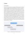
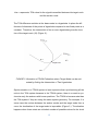
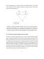
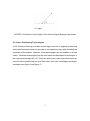
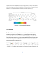
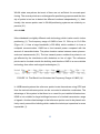
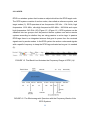
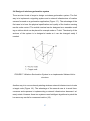
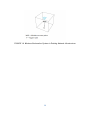
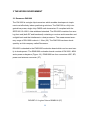
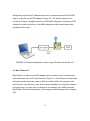
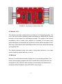
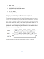
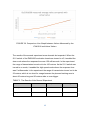
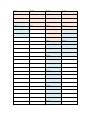
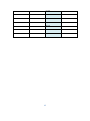
Niina Mäkinen
INDOOR POSITIONING WITH A VIEW TO TEAM SPORT TRACKING
INDOOR POSITIONING WITH A VIEW TO TEAM SPORT TRACKING
Niina Mäkinen
Bachelor’s Thesis
Spring 2015
Degree program in Information Technology
Oulu University of Applied Sciences
ABSTRACT
Oulu University of Applied Sciences
Information Technology
Author: Niina Mäkinen
Title of thesis: Indoor Positioning System with a View to a Team Sport Tracking
Supervisor: Pekka Alaluukas
Term and year of completion: Spring 2015
Pages: 49
The need for indoor positioning is emerging but the expected breakthrough has
not happened so far. The lack of accuracy, cost effectiveness and suitability for
all kinds of use cases have been the main problems with current solutions. Even
though there are such amazing indoor positioning systems, none of them has
stood out like GPS in outdoor environments. This document opens up a little bit
the world of indoor navigation and points out the current issues of the most used
indoor positioning systems.
The objective of this Bachelor’s thesis was to find out the most proper design for
a future sport tracking indoor positioning system. The document covers well considered technologies, methods and algorithms used in current indoor positioning
systems. This paper also provides an experimental evaluation of an ultra-wideband-based indoor positioning system. The evaluation was done for Decawave’s
EVK1000 evaluation boards. During the work the most suitable technology, methods and algorithms for sport tracking system were selected and the future indoor
positioning system was designed. This Bachelor’s thesis can be used as a baseline of the implementation of the ultra-wideband-based indoor positioning system.
Keywords: Indoor positioning, sport tracking, ulta-wideband, Decawave
3
CONTENTS
ABSTRACT
47
CONTENTS
47
TERMS AND ABBREVIATIONS
47
1 INTRODUCTION
9
2 THEORY
10
2.1 Classification
10
2.2 Methods used in Indoor Positioning Systems
11
2.2.1 Time of Arrival (TOA)
11
2.2.2 Time Difference of Arrival (TDOA)
12
2.2.3 The Received Signal Strength Indicator (RSSI)
14
2.2.4 The Angle of Arrival (AOA)
16
2.3 Indoor Positioning Technologies
17
2.3.1 Non-radio Technologies
19
2.3.2 Radio Signal Technologies
22
2.4 Design of wireless geolocation system
27
3 THE WORK ENVIRONMENT
29
3.1 Decawave DW1000
29
3.1 Bus Pirate v3.6
30
3.2 Ubuntu 14.10
31
3.3 Minicom
31
4 CONFIGURATION
32
5 TESTING
34
5.1 Hypothesis
34
5.2 The First Experiment
34
5.3 The Second Experiment
36
5.4 The Third Experiment
37
5.5 Results
38
6 CONCLUSION
44
7 REFERENCES
47
4
TERMS AND ABBREVIATIONS
Anchor node
An anchor node is a party which communicates via a radio signal with the target node
and its location is known. Also known as reference point located to a ceiling or on top of
the positioning area
Attenuation
Attenuation is a general term that refers to
any reduction in the strength of a signal
Bluetooth
A wireless technology that enables communication between Bluetooth-compatible devices for short-range (typically less than 30
meters) connections
Fingerprinting
A fingerprinting algorithm is a procedure
that maps a large data item to a much
shorter bit string
GLONASS
A Global Navigation Satellite System is a
space-based satellite system operated by
the Russian Aerospace Defense Forces
GPS
A Global Positioning System is a satellite
navigation system used to determine the
ground position and velocity in an outdoor
environment
Linux
An operating system, based on UNIX, that
runs on many different hardware platforms
5
and whose source code is available to the
public
LOS
Line of Sight is an unobstructed view from a
transmitter to a receiver. The accuracy of
the radio technologies relies on the LOS between nodes
MISO
Master In Slave Out (MISO) - Slaves generates MISO signals and the recipient is the
Master
MOSI
Master Out Slave In (MOSI) - MOSI signal
is generated by the Master, the recipient is
the Slave
Multi-paradigm language
A multi-paradigm programming language is
a programming language that supports
more than one programming paradigm. In
other words a language that supports multiple programming language styles
NLOS
A non Line of Sight radio transmission
across a path that is partially obstructed,
usually by a physical object
OSI
The Open Source Initiative is a California
public benefit corporation. In brief, they approve Open Source licenses
RFID
Automatic identification technology which
uses radio-frequency electromagnetic fields
to identify objects carrying tags when they
come close to a reader
6
SPI
A Serial Peripheral Interface is a hardware/firmware communications protocol developed by Motorola and later adopted by
others in the industry
SPICS
The clock speed of the Serial Peripheral Interface
Target node
A target node is another party which communicates with anchor nodes trying to find
out its location. Target node can be passive
or active. Also can be known as mobile terminal located to a positioning target
Triangulation
A method of finding a distance or location
by measuring the distance between two
points whose exact location is known and
then measuring the angles between each
point and a third unknown point
Trilateration
A method of determining the relative positions of three or more points by treating
these points as vertices of a triangle or triangles of which the angles and sides can be
measured
Ultrasonic
Ultrasound is an oscillating sound pressure
wave with a frequency greater than the upper limit of the human hearing range
Unix
An operating system written in C programming language developed in the 1970s
7
UTF-8
Universal Character Set (U) Transformation
(T) Format (F)—8-bit is a character encoding capable of encoding all possible characters in Unicode. The encoding is variablelength and uses 8-bit code units
WLAN
A wireless networking technology that allows computers and other devices to communicate over a wireless signal
8
1 INTRODUCTION
The last decades have seen the revolutionary development in positioning systems. Especially, the development of outdoor positioning systems has been significant. The indoor positioning systems have become very popular in recent
years but still there is a lot to further develop them. Some indoor positioning systems have been successfully used in different types of tracking or navigation purposes. However, none of the current indoor positioning systems have become
the most useful for any type of use cases like GPS in an outdoor environment.
GPS is not suitable for indoor positioning systems because the attenuation
caused by roofs and walls affects the localization estimation. Therefore, the old
indoor positioning systems such as magnetic positioning and inertial positioning
systems, which have many advantages, have taken place early on. However,
these technologies have also several disadvantages which caused the development of indoor positioning systems based on radio technologies.
This document provides an overview of the most used radio and non-radio technologies which could be proper for a sport tracking indoor positioning system.
Different technologies, methods and algorithms were explored and evaluated
during the work. This paper also gives a sight how to test and configure
Decawave’s EVK1000 evaluation board. The main objective of this work was to
discover a proper technology, methods and algorithms for a sport tracking indoor
positioning system and do an experimental evaluation for the selected device.
The evaluation of EVK1000 evaluation board was necessary for further development.
9
2 THEORY
2.1 Classification
The need for indoor positioning is emerging but developers have not yet implemented an enough accurate and suitable solution for all kinds of use cases (1).
GPS and GLONASS are well-known global positioning systems for outdoor environments, but there is not such a system for an indoor environment (2). Indoor
positioning systems can be classified into two groups, global and local positioning
systems. In the global positioning system (GPS) the mobile can find its own position on the globe. The local positioning system (LPS) is a relative positioning
system which can be classified into two subcategories called as a self- and remote positioning. The self-positioning system allows a target to find its position
by using the static coordination points at any given time and location. An example
of self-positioning systems is the inertial navigation system. In remote positioning
systems the system finds the reference points which are related to its own location points in the positioning area. Those points can be static or dynamic. Remote
positioning systems are divided into two groups, active and passive target remote
positioning systems (3) (Figure 1.).
FIGURE 1. Classification of the Positioning Systems
10
2.2 Methods used in Indoor Positioning Systems
By using radio signal technologies, there are three location metrics used in the
wireless indoor positioning to estimate the direction of the received signal or distance. The angle of arrival (AOA) measures the arrival angle of the received signal in direction-based systems. In distance-based systems the distance can be
estimated by using the received signal strength (RSS), the carrier signal phase
of arrival (POA) or the time of arrival (TOA) of the received signal (4). In order to
obtain more accurate information about the position of the target node, some positioning systems combine two or more position related parameters (5). The most
commonly used techniques which can be used to determine the metrics are trilateration, triangulation and fingerprinting (6). The two major sources of errors in
the location metrics in the indoor environment are no LOS (NLOS) conditions due
to a shadow fading and multipath fading (4).
2.2.1 Time of Arrival (TOA)
The time of arrival of the received signal is the most important parameter in an
accurate indoor positioning system (7). The time of arrival estimation allows the
measurement of distance in an indoor positioning system. In the TOA method the
anchor nodes use a triangulation to localize the target node. The anchor nodes
can be static or dynamic. It is assumed that the positions of all static anchor nodes
are known. If the anchor nodes are dynamic, there is a need to use GPS to localize the anchor nodes all the time. TOA requires the anchor nodes and target
nodes to work synchronized (3).
The estimation of TOA requires a very accurate timing reference at the target
node which needs to be synchronized with the clock at the anchor nodes. The
distance between a target node and an anchor node can be obtained by multiplying the TOA with the speed of light (8). A small timing error in the indoor positioning system which uses the TOA may cause a large calculation error of the distance. When running the system, each transmitted signal needs to be labeled
11
with own timestamp in order to determine the time when the signal was initiated
at the target node (3). The TOA value can be estimated by the following formula:
𝐷 = 𝑐𝑡
FORMULA 1. 𝐷 represents distance in meters,
𝑐 represents the speed of light in m/s,
𝑡 represents time in seconds (9)
The advantage of the TOA method is that there are already well developed timing
based multiple access schemes, which allow the high-accurate TOA estimation.
The disadvantages of the TOA is that all the units need to be synchronized with
each other in a system but synchronization is difficult and expensive to use for
wireless radio systems (8).
2.2.2 Time Difference of Arrival (TDOA)
The time difference of arrival method is based on the measurement of the difference in time between the signals arriving at two anchors. It is assumed that using
this method the positions of the anchor nodes are known. In the TDOA, all anchor
nodes receive the same signal transmitted by the target node (3). A perfect example of a TDOA positioning system is the GPS. The GPS satellites are synchronized by means of using atomic clocks and monitoring through the ground control
segment (8). Atomic clocks are extremely expensive so they are not quite suitable
for indoor positioning systems.
One way to estimate the TDOA is to first estimate the TOA for each signal transmitted between the target node and an anchor node, and then to define the difference between the two estimated values (Formula 2.) (5).
𝜏 𝑇𝐷𝑂𝐴 = 𝜏1 − 𝜏2
FORMULA 2. The 𝜏 𝑇𝐷𝑂𝐴 represents TDOA estimation and
12
the 𝜏𝑖 represents TOA value for the signal transmitted between the target node
and the anchor node
The TOA difference solution at the base nodes is a hyperbola. In plane the difference of distances of the points of hyperbola compared to two fixed points is a
constant. Therefore, the intersection of two or more hyperbolae gives the location of the target node (10) (Figure 2.).
FIGURE 2. Illustration of TDOA Estimation where Target Node can be estimated by finding the Intersection of Two Hyperbolae
Synchronization in a TDOA system is less expensive than synchronizing all the
units in the TOA system because in the TDOA system, there is a need to synchronize only the anchors with known positions. The TDOA is less accurate than
the TOA system if they are using the same system geometry. For example, if in
some case the vectors between the anchor nodes and the target node form a
cone, the localization of the target node is impossible (Figure 3.). The situation
happens when there exists an unlimited number of possible values for the clock
13
bias corresponding to an unlimited number of possible positions of the target
node. However, the TOA method is suitable for solving this type of cone symmetry positioning problem (8).
FIGURE 3. Geometry Symmetric Problem Case in Indoor Positioning System
where the Anchor Nodes (A1, A2, A3, A4) and the Target Node (T1) form a 3DDimensional Cone. By using the TDOA Method the Problem is Unsolvable but
Instead of using the TOA Technique the Problem Case is possible to solve.
2.2.3 The Received Signal Strength Indicator (RSSI)
The power of a signal travelling between two nodes contains a signal parameter
which is valuable information for estimating a distance between the nodes (5).
RSS can be equivalently reported as the squared magnitude of the signal. It can
be related to positioning purposes if its path loss model is known (8). The RSSI
method is similar to the TOA method because it also uses a triangulation to localize the target node (Figure 4.). However, instead of using the time of arrival,
the system uses the received signal strength. The strength of the received signal
determines the distance travelled by the signal (7). Usually, the RSSI method is
used with RF signals such as WLAN or Bluetooth (11).
14
One of the disadvantages of the RSS method is shadowing and a small scale
channel effect causing the random deviation from the mean received signal
strength, therefore the technique is less accurate than other techniques (7). The
following formula can be used to estimate the effect of multipath fading and shadowing:
𝑃𝐿 = 𝑃𝐿0 + 10log10 (𝑑 𝑛 ) + 𝑠
FORMULA 3. 𝑃𝐿 represents the total Path Loss between the Receiver and
Transmitter (must be bigger than zero),
𝑃𝐿0 represents the reference path loss in dB when distance is 1 meter and this
must be specified as greater than or equal to zero,
𝑑 represents the distance between the transmitter and receiver in meters,
𝑛 represents the path loss exponent for the environment,
𝑠 represents the standard deviation associated with the degree of shadow fading present in the environment in dB (9)
Another disadvantage is that RSS needs an accurate global reference power for
all positions because an antenna does not transmit signals with equal power in
all directions. The RSS method is not suitable for large buildings because it highly
reduces the accuracy. The RSS technique is cheap and easy to obtain with lowcomplexity algorithms. Clock bias do not exist in RSS systems therefore there is
no need for an expensive time synchronization (8).
15
FIGURE 4. The d represents the Distance in Error-free Case between Center
Node and the Target Node located on the Circle
2.2.4 The Angle of Arrival (AOA)
The angle of the arriving signal can be estimated by estimating the AOA parameter of a signal traveling between the nodes (5). To estimate the angle of the
received signal requires antenna arrays at the target node. The AOA offers complementary technique beside the RSS technique by using directional information
(8). Like in the TOA and the TDOA also in the AOA method all anchor nodes
should be known. However, the AOA method requires only two anchors along
with two AOA measurements (3).
The first advantage of the AOA technique is that there is no need for the expensive time synchronization since the AOA of one anchor-receiver pair is obtained
using the (pseudo)range differences of multiple antenna components at the same
receiver (8). However, this method causes higher cost, complexity and power
consumption compared with other methods (3).
16
FIGURE 5. Estimation of the Angle of the Arriving Signal Between two Nodes
2.3 Indoor Positioning Technologies
In the indoor positioning non-radio technologies such as a magnetic positioning
and inertial measurements can provide an increased accuracy and decrease the
expenses of the system. However, these technologies are not suitable in all use
cases. Wireless technologies are the most used and developed technologies in
the indoor positioning field (12). There are quite many radio signal technique options for indoor positioning but all of them have their own advantages and disadvantages (see figure 6 and figure 7).
17
FIGURE 6. Accuracy of Different Positioning Systems in 2007 (13)
FIGURE 7. Overview of Indoor Positioning Systems (14)
18
2.3.1 Non-radio Technologies
A number of different types of non-radio technologies are used in indoor positioning such as ultrasound, inertial systems, imaging, infrared, etc. (15) This paper covers the most used non-radio technologies in localization.
2.3.1.1 Magnetic Positioning
The magnetic positioning is a classic way of positioning tracking. It offers a high
accuracy positioning because it does not require the maintenance on line of sight
(LOS) between the anchor and target nodes (16). The magnetic positioning utilizes surrounding generated magnetic fields. Magnetic fields can be generated
either from permanent magnets or from coils. It is also possible to combine an
electric field and a magnetic field for positioning purposes (14).
The best advantage of the magnetic field positioning is that there is no need for
deploying infrastructure (17). Implementing the magnetic positioning system is
relatively cheap compared with other positioning systems. The sensors are small
therefore they do not need much space. The magnetic –based positioning systems offer a multi-position tracking (16). Using fingerprinting gives a more accurate estimation in magnetic positioning. Fingerprinting is useful if a signal propagation is unpredictable or a direct line-of-sight propagation is not typical (17). The
disadvantage of the magnetic-based system is that there is only a limited coverage range. Increasing the coverage range area requires further development
(16). Also, electronic devices or moving objects containing ferromagnetic materials may affect the magnetic field and therefore cause an error in estimation. Additionally, the intensity data of the magnetic field consist of only three intensities
in X, Y and Z directions (17).
19
2.3.1.2 Inertial Navigation
Inertial navigation systems (INS) are sophisticated autonomous, electromechanical systems which supply the position, velocity, and attitude of the object in which
they are mounted. Nowadays INS is used in many different applications including
the navigation of an aircraft, tactical and strategic missiles, submarines, ships
and spacecraft (18). The operation of INS is based on the laws of classical mechanics formulated by Isaac Newton. Newton’s laws tell us that the motion of a
body will continue uniformly in a straight line unless disturbed by an external force
acting the body. The laws also tell us that this force will produce a proportional
acceleration of the body (19).
In INS accelerometers and gyroscopes provide an ability to track the position and
orientation of a tracking object relative to a known starting point, orientation and
velocity. Inertial measurement units (IMUs) usually contain three orthogonal rategyroscopes and three orthogonal accelerometers (Figure 8.). Orthogonal rategyroscopes and orthogonal accelerometers measure the angular velocity and linear acceleration respectively in the system (18). The inertial navigation system
relies on the availability of the knowledge of the starting point. In order to navigate
it is necessary to keep track of the direction of the accelerometer (Figure 9.).
Gyroscopic sensors are used to determine the orientation of the accelerometer
at all times (19).
20
FIGURE 8. Stable Platform of Inertial Measurement Unit (9)
FIGURE 9. The Body and Global Frames of Reference of Inertial Navigation
System (9)
21
2.3.1.3 Ultrasonic
In nature there are living creatures which have independently evolved bio sonar
systems to navigate and locate and catch prey. Toothed whales and bats are able
to operate in darkness but also communicate with a same species comrade by
ultrasonic (20). The frequency range of ultrasonic is from 20 kHz to 10 MHz (Figure 10.). The velocity of sound waves is about 340 m/s whereas the speed of
radio waves is 300,000,000 m/s (15).
FIGURE 10. The Black Line illustrates the Frequency Range of Ultrasonic (14)
Slower velocity makes it a lot easier to estimate the time of flight measurement
(15). Ultrasonic offers a low cost solution which can also be used in indoor positioning. One of the disadvantages of an ultrasonic system is a loss of signal due
to the interference with obstacles on line of sight. Sometimes the signal can also
turn to be false because of the reflection or measurement can face interference
from other high frequency sounds such as keys jangling (12). Ultrasonic is also
sensitive to temperature variations and multipath signals which makes it unsuitable to some use cases (11).
2.3.2 Radio Signal Technologies
Radio signal technologies are the most developed technologies in indoor positioning field at the moment. However, the radio positioning systems are often
more expensive compared to non-radio-based positioning systems (17). The radio frequency range is around 3 kHz to 300 GHz (Figure 11.). The most difficult
parts of the development of the radio-based indoor positioning system are multipath and shadow fading. The functionality of the radio-based indoor positioning
22
system relies on the availability of a line of sight (LOS) (4). Also, if the chosen
radio technology needs the pre-installation of infrastructure or fingerprinting database etc., the implementation is difficult, slow and expensive (1).
FIGURE 11. Electromagnetic spectrum
2.3.2.1 Bluetooth
The Bluetooth is a short-range data communication protocol which is also
known as the IEEE 802.15 standard (21). The range band of the radio frequency of the Bluetooth is from 2.4 to 2.485 GHz (22) (Figure 12.). The Bluetooth positioning system is one of the network-based positioning systems and
can also be categorized as LPS. Bluetooth devices contain mini-cells which
have a strong effect on accuracy (21).
FIGURE 12. The Black Line illustrates the Frequency Range of Bluetooth (14)
23
Bluetooth technology is suitable for providing some limited communication with
the positioning information but it has also an issue. The disadvantage of Bluetooth technology is that the architecture of the system requires a lot of expensive receivers. The accuracy of Bluetooth indoor positioning system depends
strongly on the number and size of the cells in device (21).
2.3.2.2 WLAN
A wireless local area network is a typical network based LPS (21). WLAN is a
wireless computer network that links two or more devices using a wireless distribution method (1). The WLAN which is also known as the Wi-Fi or the IEEE
802.11 standard is a higher bandwidth communication protocol than Bluetooth
(21). WLAN operates at 2.4 GHz, 3.6 GHz, 4.9 GHz, 5 GHz, and 5.9 GHz bands
(23) (Figure 13.). The range of the radio frequency of WLAN and Bluetooth overlaps at 2.4 GHz. However, neither WLAN nor Bluetooth was implemented to deal
with the interference that each creates for the other. Overlapping may cause little
issue when developing indoor positioning system with either of these technologies (24). WLAN is an older technology than Bluetooth therefore it is a little bit
more sophisticated (21).
FIGURE 13. The Black Line illustrates the Frequency Range of WLAN (14)
In emergency situations WLAN is often vulnerable because it requires a local
infrastructure. However, it has been used for indoor positioning in hospitals but
for an accurate positioning the signal strength measurements and triangulation
are not sufficient. Advanced methods such as fingerprinting might be a solution
but collecting a database of offline points is quite time consuming. Nowadays,
24
WLAN exists everywhere but most of them are not sufficient for accurate positioning. The access points are not designed for positioning purposes and the density of points is too low to detect the different locations independently (1). Additionally, the access points used in WLAN positioning systems are relatively expensive (21).
2.3.2.3 UWB
Ultra-wideband is a slightly different radio technology which is also used in indoor
positioning (1). The frequency range of UWB is from 3.1 GHz up to 10.6 GHz
(Figure 14.). It has a large bandwidth (>500 MHz) which enables it to have a
multipath communication. UWB has a low transmit power compared with the
amount of transmitted data. The pulse duration varies between some picoseconds and nanoseconds (21). The low transmit power enables the pulses to not
get affected by the interference with obstacles on line of sight. The reference
points can be located outside the building and therefore UWB is a more reliable
technology than other radio signal technologies (1).
FIGURE 14. The Black Line illustrates the Frequency Range of UWB (14)
In UWB-based systems the reference points locate themselves using GPS and
thus the tracked reference points can be converted to absolute coordinates. The
advantage of this system is that there is no need for pre-installed infrastructure.
UWB is not suitable for large buildings because of a limited transmission range
of signals. Another disadvantage is that reference points need to be placed relatively evenly around the building which makes the technique impractical or even
impossible (1).
25
2.3.2.4 RFID
RFID is a wireless system that locates an object which has the RFID target node.
The RFID system consists of anchor nodes, also called as reference points, and
target nodes (3). RFID operates at low frequencies 125 kHz – 134.2 kHz, high
frequencies 13.56 MHz, ultra-high frequencies 860 MHz - 960 MHz and super
high frequencies 2.45 GHz (25) (Figure 15.) (Figure 16.). RFID systems can be
classified into two groups such as passive remote systems and active remote
systems according to whether they are using passive or active tags. In passive
RFID tags there is an integrated antenna that gets its power from the received
signals sent by anchor nodes. In the RFID system the anchor nodes send signals
with a specific frequency to keep the RFID tags activated as long as it is needed
(3).
FIGURE 15. The Black Line illustrates the Frequency Range of RFID (14)
FIGURE 16. The Electromagnetic Spectrum with the Frequency Bands of the
RFID Systems
26
2.4 Design of wireless geolocation system
There are two kinds of ways to design a wireless geolocation system. The first
way is to implement a signaling system and a network infrastructure of location
sensors focused on a geolocation application (Figure 17.). The advantage of the
first case is to have the physical specification and quality of the location sensing
results under control. The mobile terminal can be designed as a wearable small
tag or sticker which can be placed for example under a T-shirt. The density of the
anchors of the system is in designer’s hands so it can be changed easily if
needed.
FIGURE17. Wireless Geolocation System in an implemented Network Infrastructure
Another way is to use an already existing wireless network infrastructure to locate
a target node (Figure 18.). The advantage of the second case is to avoid timeconsume and expenses in implementing a network infrastructure because it already exists. However these two systems need intelligent algorithms to patch the
low accuracy results for measured metrics (18).
27
FIGURE 18. Wireless Geolocation System in Existing Network Infrastructure
28
3 THE WORK ENVIRONMENT
3.1 Decawave DW1000
The DW1000 is a single chip transceiver which enables developers to implement cost effectively indoor positioning solutions. The DW1000 is a fully integrated low power, single chip CMOS radio transceiver IC compliant with the
IEEE 802.15.4-2011 ultra-wideband standard. The DW1000 consists of an analog front-end (both RF and baseband) containing a receiver and transmitter and
a digital back-end that interfaces to a host processor. The measurement accuracy range of DW1000 is about +/-10cm (26). The DW1000 has been developed by an Irish company called Decawave.
DW1000 is attached to the EWB1000 evaluation board which can be used easily in development. The EWB1000 evaluation board consists of DW1000, ARM
and a power subsystem (Figure 19.). EWB1000 has four connectors USP, SPI,
power and antenna connector (27).
FIGURE 19. Logical View of EWB100 (27)
29
During the project the SPI channel was used to communicate with a DW1000
chip by computer via an SPI-adapter (Figure 20.). S2 switch needed to be
turned off to have a straight channel to a DW1000 subsystem. Switching off S2
enabled to avoid connection to the ARM subsystem which would have been
pointless in this case.
FIGURE 20. External Application control using SPI External Header (27)
3.1 Bus Pirate v3.6
Bus Pirate is an open source SPI adapter which can be used to communicate
with electronics from a PC serial terminal (Figure 21.). Bus Pirate v3.6 was used
during the project because it has an SPI bus traffic sniffer, the manual is well
documented, cost effective, open source and scriptable from a Python programming language. It is also easy to connect to a computer via a USB connector.
Bus Pirate v3.6 was developed by a US company called Dangerous Prototypes
(28).
30
FIGURE 21. Bp Protocol of Bus Pirate (28)
3.2 Ubuntu 14.10
The software itself was implemented on an Ubuntu 14.10 operating system. Ubuntu is an open source operating system developed by Canonical Ltd. Ubuntu
belongs to a Unix-based Linux distribution package. The mission of the Ubuntu
development was to create a free software to everybody. All volunteers were
gathered together and therefore the first Ubuntu version saw the daylight in 2004.
After many years Ubuntu still is and always will be free to use, share and develop
to everybody (29).
The Ubuntu operating system was used in this project because it is an open
source operating system and easy to set up.
3.3 Minicom
Minicom is a serial communication program for Linux operating systems. The
serial communication programs are used to send data one bit at the time over
computer bus (30). Minicom was used as a communication tool between the
computer and the hardware device EVK1000 in this project.
31
4 CONFIGURATION
The configuration started by installing a Minicom serial communication program
on the Ubuntu operating system. After installation, the configuration of the USB
port for Minicom needed to be set and saved as default. When the configuration
was completed, the Bus Pirate SPI adapter was required to connect with the computer via the USB bus. Before connecting the EVK1000 with the SPI adapter it
was required to configure the EVK1000 so that straight communication with the
DW1000 was possible. At first all the S1 dips of the EVK1000 board had to be
set to off mode to enable the SPI connection. Additionally the EVK1000 dips
needed to be set so that the transmission speed of packages was faster than the
default to speed up the testing. Finally, the small cords of the SPI adapter were
required to connect with right spikes on the EVK1000 board (Figure 22.). If some
of the cords would have connected with a wrong spike, it would have caused a
short circuit in the worst case.
Figure 22. SPI Adapter connected with EWK1000 Evaluation Board
After completing all hardware connections, it was possible to start setting up SPI
settings in Minicom prompt. The working SPI settings were:
32

speed: 1MHz

clock polarity: idle low *default

clock output edge: active to idle *default

clock phase: middle * default

CS: /CS *default

output type: normal
After going through all settings the SPI channel was ready for use.
The development started with the MISO and MOSI testing to figure out if the connections and settings were set up right. MISO stands for Master In, Slave Out
which means to generate the Slave line for sending data to the master. Mutually
MOSI means Master Out, Slave In and means to generate the Master line for
sending data to the peripherals. By sending an index value to master, the responds were exactly the ones they were supposed to be and therefore the configurations were successful (Figure 23.).
FIGURE 23. MOSI and MISO Non-indexed Read of Device ID Register
33
5 TESTING
The aims of the testing were to find out how accurate the measurement performed by two EWB1000 evaluation boards in different circumstances. Is there
a couple of factors which need be considered as adverse factors on the measurement accuracy such as distance, velocity, temperature and objects placed
on line of sight. The adverse factors need to be taken into account because it is
assumed that they have a strong effect on accuracy. In this document just velocity and distance issues were tested.
5.1 Hypothesis
According to the sources found about ultra-wideband, it is assumed that the UWB
technology should not be suitable for a long distance measuring because of its
limited transmission range of signals. Therefore the measurement accuracy
should decrease while lengthening the distance between two nodes. It was also
mentioned in one of the sources that the accuracy of the ultra-wideband also
decreases if there are any objects disturbing the line of sight of the radio signal.
Additionally, it is assumed that velocity effects on descending range of ultra-wideband signal.
5.2 The First Experiment
The first experiment was performed indoors using two EVK1000 boards, two laptops, a tape measure, a Shealt application on Galaxy S4, a pen and a paper.
During the first experiment the task was to evaluate the accuracy of the EWB1000
boards in indoor circumstances where the temperature varied from +8 °C to +11
°C and the humidity from 52 % to 44 %. The main objective of the test was to
measure how accurate the measurement is in a static state. At first the tape
measure was placed on a hallway and 2m, 5m, 10m, 20m, 30m, 40m and 50m
34
points were highlighted. One of the EWB1000 boards was placed in 0m and another was moved to the highlighted points step by step (Figure 24.).
FIGURE 24. The Tape Measure was placed between two Nodes
Every highlighted point was measured 5 times by the EWB1000 board and
marked to a datasheet. The EWB1000 interface displays AVG and AVG8 values,
however in this case only AVG8 was used. The EWB1000 board, which was
placed on different points, needed to be set carefully because even a little offset
might have caused a bigger error value (Figure 25.). The EWB1000 boards were
required to be connected to computers via a USB cable because they do not have
their own power source.
35
FIGURE 25. Measuring the Distance
5.3 The Second Experiment
The second experiment was performed outdoors using two EVK1000 boards by
turning the response time of the EVK1000 boards from a slow to a high speed.
The objective of this experiment was to find out how much the high speed mode
decreases the range of transmission of the signal. In the manual of the
EVK1000 it is mentioned that when decreasing the response time from 150 milliseconds to 5 milliseconds, the range of line of sight decreases.
At first the EWB1000 evaluation boards were configured to be in a slow speed
mode where the response time was 5 milliseconds. The slow speed mode was
managed by turning the S1-2 switch to on state. The S1-2 switch is used to enable fast two-way ranging where the response time is set to 5 milliseconds. If
turned off, the response time is set to 150 milliseconds (Figure 26.). After the
first trial the EWB1000 boards were configured to a high speed mode where the
response time was set to 5 milliseconds by turning the S1-2 switch to off state.
The temperature was around +0 °C in the experiment environment.
36
FIGURE 26. S1-2 Pin enabled to change Time of Response
5.4 The Third Experiment
During the third experiment the accuracy of the active target in outdoor circumstances was explored when the response time of the EWB1000 evaluation
boards were increased. This experiment was performed also outdoors using
two EVK1000 boards, two laptops, a video camera, a car, a pen and a paper.
One of the EVK1000 boards was located as a static anchor node and other was
placed as a dynamic tag into the car. The objective of this experiment was to
find out if it is enough to increase the response time from 150 milliseconds to 5
milliseconds to be able to track the active tag node when it has a high velocity
(Figure 27.).
FIGURE 27. Tracking Active Tag in High Velocity
37
A video camera was used in this experiment to gather the data displayed on the
screen of the EVK1000 evaluation board. The data was valuable to evaluate
how quickly the EVK1000 responds to a transmitted signal. The video recording
method was used because there was not yet a functionality in the system which
would have stored the data to the server. The video record was easy to evaluate afterwards (Figure 28.).
FIGURE 28. Experiment Equipment of the Third Experiment
5.5 Results
The first experiment was carried out as planned and the results gave more information about the suitability of the EWB1000 evaluation board for further development. The results were recorded in one decimal place of accuracy. The results of
measurements of the first experiment were better than were expected. Without
any distraction on line of sight, the measurements of EWB1000 boards were
enough accurate. As regarding to the Sparkline diagram, the measurements
where the distance was short between two nodes were descending compared
with the actual values (Table 1.). When the distance was around 30 meters, the
measurement turned out to be exact. As the distance was lengthened from 30
meters, the results were ascending compared with the actual values.
38
TABLE 1. The Results of Measurements by Decawave EWB1000 Device compared to the Actual Values
tape measure
(m)
2
5
10
20
30
40
50
Decawave, measured value (m)
test 1
1,8
4,9
9,8
19,8
30
40
50,4
test 2
1,8
4,9
9,8
19,9
30
40,1
51,1
test 3
1,8
4,9
9,8
19,8
30
40,2
51
test 4
1,8
4,9
9,8
19,8
30,1
40,1
50,3
test 5
1,8
4,9
9,8
19,8
30
40,2
50,3
AVG
Sparkline diagram
1,8
4,9
9,8
19,8
30,0
40,1
50,6
Although a Sparkline diagram shows a little deviation from the actual values, the
accuracy was proven to be enough accurate (Figure 29.). In the first experiment
the biggest measured deviation was 1,1 centimeters in 50 meters and the smallest in 30 meters in where the deviation was nearly zero. The first test measurements in short distances demonstrate that the EWB1000 evaluation board might
have been set to display a little lower value to measure a more accurate result
in longer distances.
There are also some adverse factors which need to be taken into account when
interpreting the results. In longer distances there is a bigger probability to have
a distraction on line of sight which affects on accuracy by ascending the value.
Additionally there is no evidence of having the tape measure placed exactly on
a straight line. Placing another EWB1000 board on highlighted points might also
have caused a little offset because the board was placed on the points by hand.
39
FIGURE 29. Comparison Line Graph between Values Measured by the
EVK1000 and Actual Values
The results of the second experiment were dramatic but expected. When the
S1-2 switch of the EWB1000 evaluation board was turned to off, it enabled the
slow mode where the response time was 150 milliseconds. In the experiment
the range of transmission turned out to be 100 meters. As the S1-2 switch was
turned to on mode, it enabled the high speed mode where the response time
was 5 milliseconds. In the experiment the range of transmission turned out to be
22 meters, which is too short for usage because the planned tracking area is
about 60 meters long and 30 meters wide or even bigger.
TABLE 2. The Results of the Second Experiment
Mode
S1-2 switch
Response time
Range
Slow speed
off
150 ms
100 m
High speed
on
5 ms
22 m
40
The third experiment focused on the velocity issue when the device is in the
high speed mode. The video camera was used to gather the data during the
drive. In all trials when the target was in initial point, it was in a rest state and
started to accelerate to get the speed up to 20km/h before passing the anchor
node. The first trial started in 100 meters away from the anchor node and the
velocity of the target node was around 20km/h when the target passed the anchor. The device detected the target in 16,53 meters and lost the sight after
9,33 meters (Table 3.). In the second trial the target node started from 21,58
meters and did not reach 20km/h before the anchor node. The recording was
stopped at 3,53 meters when the car was exactly aligned with the anchor node.
In both trial three and four the target node started at around 22 meters and it
was recorded till the end. Also, in these two trials the velocity did not quite reach
to 20km/h. In trial three the last distance in the end was 54,67 meters and in the
trial four it was 66,25 meters.
The data gathered during the third experiment shows that the data flow is not
constant (Table 3.). Especially, in the fourth trial the anchor lost the target after
16,25 meters and detected it again in 66,25 meters. Comparing the first trial to
others it can be considered that the anchor needs a pre response before starting the tracking. In the first trial the target node was placed far away from the
anchor node and the anchor node did not detect it before start. The target
reached 20km/h therefore it was not detected until in 16,53 meters. The most
accurate trial was the third one which does not include long intervals between
the measurements.
TABLE 3. Recorded Data when the Target Node had Velocity of 20km/h
Trial 1th (100 m)
Trial 2nd (21,58 m)
Trial 3rd (22,29m)
Trial 4th (21,81m)
16,53 m
21,58 m
22,29 m
21,81 m
13,74 m
19,62 m
22,28 m
20,08 m
11 m
18,23 m
22,12 m
17,24 m
8,40 m
16,61 m
21,71 m
15,18 m
41
5,82 m
14,80 m
20,95 m
12,18 m
3,45 m
10,72 m
15,66 m
10,14 m
1,49 m
8,40 m
12,00 m
7,46 m
2,24 m
5,99 m
9,87 m
4,65 m
4,35 m
3,53 m
7,60 m
1,87 m
6,75 m
5,23 m
1,59 m
9,33 m
2,78 m
4,43 m
1,01 m
7,56 m
2,76 m
10,37 m
5,36 m
13,30 m
8,07 m
16,28 m
10,82 m
66,25 m
13,67 m
16,24 m
18,61 m
20,81 m
23,11 m
34,90 m
37,34 m
39,69 m
41,95 m
44,20 m
46,30 m
48,27 m
49,91 m
42
51,29 m
52,45 m
53,37 m
54,00 m
54,40 m
54,65 m
54,67 m
43
6 CONCLUSION
Currently, radio technologies seem to be a better option for sport tracking system than non-radio technologies because they are more accurate in the indoor
environment. Comparing different types of radio technologies, the ultra-wideband came prominence because of the accuracy, multipath communication and
cost. The methods used with an ultra-wideband are typically the TDOA and the
AOA. The future sport tracking indoor positioning system needs for sure a pre
installation of infrastructure because it will not be able to use the already existing wireless network.
The conclusion of the experimental evaluation of the Decawave’s EVK1000
evaluation board was that it needs a custom software and better antennas to be
more accurate. The first experiment with a passive target and in a low speed
mode was better than was expected. The biggest error value was 1.1 centimeters during the first experiment. The second experiment was worse than was
expected because the range of signal decreased from 100 meters to 22 meters
when turning the slow speed mode of the response time to a high speed mode.
The shortening of the range was known but the magnitude of the change was
unexpected. In the third experiment the task was to evaluate an active target
with a maximum velocity of 20km/h. The experiment proved that the EVK1000
is not able to track at regular intervals and the longest distance for the first detected signal was around 22 meters in a sleepy mode.
The plan of the indoor positioning system was mainly based on the information
found from the sources of this document. The radio signal technology used in
this indoor positioning system will be ultra-wideband. The most suitable device
found was the Decawave’s EWK1000 evaluation board. The method which will
be used in this system is the TDOA method which draws hyperbolae curves.
The intersections of the hyperbolae curves are the coordinates of the target
node. The anchor nodes must be placed on the sides of the tracking area. The
anchor nodes do not need to be equally located on the sides but their clocks
44
need to be synchronized. Each anchor node communicates with the target
nodes and sends the information to the server where the data will be stored
(Figure 30.). On the server side the data will be processed with algorithms and
sent to a UI layer where it will be displayed to the user. The data is valuable information for example in team sport tracking.
FIGURE 30. The Plan of the Indoor Positioning System
During my Bachelor’s thesis I learned a lot about different radio and non-radio
technologies which can be used in the indoor positioning systems. They all
have different types of pros and cons which affect significantly the architecture
of the system. I also found out how to classify and compare the technologies
and methods with each other. This Bachelor’s thesis helped one software company to select the right technology and methods and evaluate the analysis for
the selected devices. In the middle of the thesis I learned how to configure and
use the SPI adapter with the EWB1000 evaluation board. I also learned how to
configure, set up and change the response mode of the EWB100 evaluation
board. This Bachelor’s thesis was interesting because the evaluated test analyses proved that some of the found theories did not quite match with the analyses. However, our test environment was not error-free and thus the claims
45
cannot be fully supported. Throughout this Bachelor’s thesis I cooperated with
my project managers and followed the instructions carefully.
If I had to do something differently, I would do the testing during the summer because now the weather was continually too bad for the devices. The testing
could have been done in an error-free environment to get more accurate results. This document holds all information from the technical perspective and it
can be used to start the implementation of the ultra-wideband –based indoor
positioning system. Overall the Bachelor’s thesis was successful and satisfactory results were achieved.
46
7 REFERENCES
1. Perttula, A. Leppakoski, H. Kirkko-Jaakkola, M. Davidson, P. Collin, J. Takala, J. 2014. Distributed indoor positioning system with inertial measurements
and map matching. IEEE Transactions on Instrumentation and Measurement.
63(11):2682-95.
2. Yayan, U. Yucel, H. Yazici, A. 2014. A Low Cost Ultrasonic Based Positioning System for the Indoor Navigation of Mobile Robots. Journal of Intelligent &
Robotic Systems.
3. Zekavat, SAR. Buehrer, R. 2011. Handbook of Position Location: Theory,
Practice, and Advances.
4. Pahlavan, K. Li, X. Mäkelä, J-. 2002. Indoor geolocation science and technology. IEEE Communications Magazine. 40(2):112-8.
5. Gezici, S. 2008. A survey on wireless position estimation. Wireless Personal
Communications. 44(3):263-82.
6. Fuchs, C. Aschenbruck, N. Martini, P. Wieneke, M. 2011. Indoor tracking for
mission critical scenarios: A survey. Pervasive and Mobile Computing. 7(1):115.
7. Ali AA, Omar A. 2005. Time of Arrival estimation for WLAN indoor positioning
systems using Matrix Pencil Super Resolution Algorithm. Proceedings of the
2nd Workshop on Positioning, Navigation and Communication, WPNC.
8. Yan, J. 2010 Algorithms for indoor positioning systems using ultra-wideband
signals. Delft University of Technology.
9. Wi-Fi Location-Based Services 4.1 Design Guide - Location Tracking Approaches [Design Zone for Mobility] - Cisco. 2008. Date of retrieval: 28.2.2015.
47
http://www.cisco.com/c/en/us/td/docs/solutions/Enterprise/Mobility/WiFiLBSDG/wifich2.html.
10. Drake, SR. Dogancay, K. 2004. Geolocation by time difference of arrival using hyperbolic asymptotes. Acoustics, Speech, and Signal Processing, 2004.
Proceedings.(ICASSP'04). IEEE International Conference on; IEEE.
11. Mautz, R. 2009. Overview of current indoor positioning systems. Geodezija
ir kartografija. 35(1):18-22.
12. Randell, C. Muller, H. 2001 Low cost indoor positioning system. Ubicomp
2001: Ubiquitous Computing; Springer.
13. Liu, H. Darabi, H. Banerjee, P. Liu, J. 2007. Survey of wireless indoor positioning techniques and systems. Systems, Man, and Cybernetics, Part C: Applications and Reviews, IEEE Transactions on. 37(6):1067-80.
14. Mautz R. 2012. Indoor positioning technologies. Habilitation Thesis, ETH
Zurich, Zurich, Switzerland.
15. Goswami, S. 2012. Indoor location technologies. Springer Science & Business Media.
16. Gu, Y. Lo, A. Niemegeers, I. 2009. A survey of indoor positioning systems
for wireless personal networks. Communications Surveys & Tutorials, IEEE.
11(1):13-32.
17. Li, B. Gallagher, T. Dempster, AG. Rizos, C. 2012. How feasible is the use
of magnetic field alone for indoor positioning? International Conference on Indoor Positioning and Indoor Navigation.
18. Woodman, OJ. 2007. An introduction to inertial navigation. University of
Cambridge, Computer Laboratory, Tech.Rep.UCAMCL-TR-696. Pages 14-15.
19. Titterton, D. Weston, JL. 2004. Strapdown inertial navigation technology.
IET. Page 2.
48
20. Wilson, M. Wahlberg, M. Surlykke, A. Madsen, P.T. 2013. Ultrasonic predator–prey interactions in water–convergent evolution with insects and bats in air?
Frontiers in physiology. Page 4. Frontiers in Physiology.
21. Renaudin, V. Yalak, O. Tomé, P. Merminod, B. 2007. Indoor navigation of
emergency agents. European Journal of Navigation. 5(3):36-45.
22. Home | Bluetooth Technology Special Interest Group. 2015. Date of retrieval 30.2.2015. https://www.bluetooth.org/en-us.
23. IEEE-SA -IEEE Get 803 Program - 802.11: Wireless LANs. 2015. Date of
retrieval 1.3.2015. http://standards.ieee.org/about/get/802/802.11.html.
24. Lansford, J. Stephens, A. Nevo, R. 2001. Wi-Fi (802.11 b) and Bluetooth:
enabling coexistence. Network, IEEE. 15(5):20-7.
25. RFID frequency ranges. 2015. Date of retrieval 2.3.2015. http://www.centrenational-rfid.com/rfid-frequency-ranges-article-16-gb-ruid-202.html.
26. Decawave | DW1000 user manual. 2014. Date of retrieval 5.3.2015.
http://www.decawave.com/sites/default/files/resources/dw1000_user_manual_2.03.pdf.
27. Decawave | EVK1000 user manual. 2014. Date of retrieval 10.3.2015.
http://www.decawave.com/sites/default/files/product-pdf/evk1000_user_manual_v107.pdf.
28. Bus Pirate - DP. 2015. Date of retrieval 11.3.2015. http://dangerousprototypes.com/docs/Bus_Pirate.
29. The leading OS for PC, tablet, phone and cloud | Ubuntu. 2015. Date of retrieval 12.3.2015. http://www.ubuntu.com/.
30. Minicom - Community Help Wiki. 2015. Date of retrieval 13.3.2015.
https://help.ubuntu.com/community/Minicom#Minicom-1.
49