Download THREE PARALLEL PROGRAMMING PARADIGMS

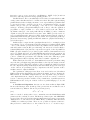
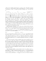
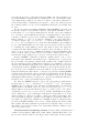
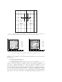
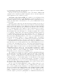
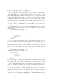
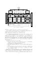
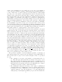
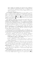
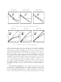
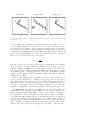
THREE PARALLEL PROGRAMMING PARADIGMS:
COMPARISONS ON AN ARCHETYPAL PDE COMPUTATION
M. EHTESHAM HAYDER∗ , CONSTANTINOS S. IEROTHEOU† , AND DAVID E. KEYES‡
Abstract. Three paradigms for distributed-memory parallel computation that free the application programmer from the details of message passing are compared for an archetypal structured
scientific computation — a nonlinear, structured-grid partial differential equation boundary value
problem — using the same algorithm on the same hardware. All of the paradigms — parallel
languages represented by the Portland Group’s HPF, (semi-)automated serial-to-parallel source-tosource translation represented by CAPTools from the University of Greenwich, and parallel libraries
represented by Argonne’s PETSc — are found to be easy to use for this problem class, and all are
reasonably effective in exploiting concurrency after a short learning curve. The level of involvement required by the application programmer under any paradigm includes specification of the data
partitioning, corresponding to a geometrically simple decomposition of the domain of the PDE. Programming in SPMD style for the PETSc library requires writing only the routines that discretize
the PDE and its Jacobian, managing subdomain-to-processor mappings (affine global-to-local index
mappings), and interfacing to library solver routines. Programming for HPF requires a complete
sequential implementation of the same algorithm as a starting point, introduction of concurrency
through subdomain blocking (a task similar to the index mapping), and modest experimentation
with rewriting loops to elucidate to the compiler the latent concurrency. Programming with CAPTools involves feeding the same sequential implementation to the CAPTools interactive parallelization system, and guiding the source-to-source code transformation by responding to various queries
about quantities knowable only at runtime. Results representative of “the state of the practice” for a
scaled sequence of structured grid problems are given on three of the most important contemporary
high-performance platforms: the IBM SP, the SGI Origin 2000, and the CRAY T3E.
1. Introduction. Parallel computations advance through synergism in numerical algorithms and system software technology. Algorithmic advances permit more
rapid convergence to more accurate results with the same or reduced demands on processor, memory, and communication subsystems. System software advances provide
more convenient expression and greater exploitation of latent algorithmic concurrency,
and take improved advantage of architecture. These advances can be appropriated
by application programmers through a variety of means: parallel languages that are
compiled directly, source-to-source translators that aid in the embedding of data exchange and coordination constructs into standard high-level languages, and parallel
libraries that support specific parallel kernels. In this paper, we compare all three
approaches as represented by “state-of-the-practice” software on three machines that
can be programmed using message passing.
Unfortunately, the development and tuning of a parallel numerical code from
scratch remains a time-consuming task. The burden on the programmer may be
reduced if the high-level programming language itself supports parallel constructs,
which is the philosophy that underlies the High Performance Fortran [26] extensions
to Fortran. With varying degrees of hints from programmers, the HPF approach
leaves the responsibility of managing concurrency and data communication to the
compiler and runtime system.
The difficulty of complete and fully automatic interprocedural dependence analysis and disambiguation in a language like Fortran suggests the opportunity for an
∗ Center for Research on High Performance Software, Rice University, Houston, TX 77005, USA,
[email protected],
† Parallel Processing Research Group, University of Greenwich, London SE18 6PF, UK,
[email protected]
‡ Computer Science Department, Old Dominion University and ICASE, Norfolk, VA 23529-0162,
USA, [email protected]
1
interactive source-to-source approach to parallelization. CAPTools [16] is such an
interactive authoring system for message-passing parallel code.
Parallel libraries offer a somewhat higher level solution for tasks which are sufficiently common that libraries have been written for them. The philosophy underlying
parallel libraries is that for high performance, some expert human programmer must
become involved in the concurrency detection, process assignment, interprocess data
transfer, and process-to-processor mapping — but only once for each algorithmic
archetype. A library, perhaps with multiple levels of entry to allow the application
programmer to employ defaults or to exert detailed control, is the embodiment of
algorithmic archetypes. One such parallel library is PETSc [3], under continuous
expansion at Argonne National Laboratory since 1991. PETSc provides a wide variety of parallel numerical routines for scalable applications involving the solution of
partial differential and integral equations, and certain other regular data parallel applications. It uses message passing via MPI and assumes no physical data sharing or
global address space.
In this study we compare the three paradigms discussed above on a simple problem
representative of low-order structured-grid discretizations of nonlinear elliptic PDEs
— the so-called “Bratu” problem. The solution algorithm is a Newton-Krylov method
with subdomain-concurrent ILU preconditioning, also known as a Newton-KrylovSchwarz (NKS) method [22]. Its basic components are typical of other algorithms for
PDEs: (1) sparse matrix-vector products (together with Jacobian matrix and residual vector evaluations) based on regular multidimensional grid stencil operations, (2)
sparse triangular solution recurrences, (3) global reductions, and (4) DAXPYs. Our
goal is to examine the performance and scalability of these three different programming paradigms for this broadly important class of scientific computations.
With relatively modest effort, we obtain similar and reasonable performance using
any of the three paradigms, suggesting that all three technologies are mature for static
structured problems. This study expands on [14] by bringing the CAPTools system
into the comparison (an important addition, since the CAPTools approach often edges
out the other two in performance) and by comparisons of the three systems on three
machines, instead of just the IBM SP.
The organization of this paper is as follows. Section 2 describes a model nonlinear
PDE problem and its discretization and solution algorithm. Section 3 discusses the
HPF, CAPTools, and PETSc implementations of the algorithm. The performance
of the implementations is compared, side-by-side, in Section 4, and we conclude in
Section 5. Our target audience includes both potential users of parallel systems for
PDE simulation and developers of future versions of parallel languages, tools, and
libraries.
2. Problem and Algorithm. Our test case is a classic nonlinear elliptic PDE,
known as the Bratu problem. In this problem, generation from a nonlinear reaction
term is balanced by diffusion. The model problem is given by
(2.1)
−∇2 u − λeu = 0,
with u = 0 at the boundary, where λ is a constant known as the Frank-Kamenetskii
parameter in the combustion context. The Bratu problem is a part of the MINPACK2 test problem collection [2] and its solution is implemented in a variety of ways in the
distribution set of demo drivers for the PETSc library, to illustrate different features
of PETSc for nonlinear problems. There are two possible steady-state solutions to
this problem for certain values of λ. One solution is close to u = 0 and is easy to
2
obtain. A close starting point is needed to converge to the other solution. For our
model case, we consider a square domain of unit length and λ = 6. We use a standard
central difference scheme on a uniform grid (shown in Figure 2.1) to discretize (2.1)
as
uij ,
i, j = 0, n
= 0,
fij (u) ≡
4ui,j − ui−1,j − ui+1,j − ui,j−1 − ui,j+1 − h2 λeui,j , otherwise
where fij is a function of the vector of discrete unknowns uij , defined at each interior and boundary grid point: ui,j ≈ u(xi , yj ); xi ≡ ih, i = 0, 1, . . . , n; yj ≡ jh, j =
0, 1, . . . n, h ≡ n1 . The discretization leads to a nonlinear algebraic problem of dimension (n + 1)2 , with a sparse Jacobian matrix of condition number O(n2 ), asymptotically in n, for fixed λ. The typical number of nonzeros per row of the Jacobian is
five, with just one in rows corresponding to boundary points of the physical domain.
The algorithmic discussion in the balance of this section is sufficient to understand
the main computation and communication costs in solving nonlinear elliptic boundary
value problems like (2.1), but we defer full parallel complexity studies, including a
discussion of optimal parallel granularities, partitioning strategies, and running times
to the literature, e.g. [12, 24]. In this study, most of the computations were done
using one-dimensional domain decomposition (shown in Figure 2.1). We also present
some results for two-dimensional blocking.
Outer Iteration: Newton. We solve f (u) = 0 by an inexact Newton-iterative
method with a cubic backtracking line search [10]. We use the term “inexact Newton
method” to denote any nonlinear iterative method approaching the solution u through
a sequence of iterates u` = u`−1 + α · δu` , beginning with an initial iterate u0 , where
α is determined by some globalization strategy, and δu` approximately satisfies the
true Newton correction linear system
(2.2)
f 0 (u`−1 ) δu = −f (u`−1 ),
in the sense that the linear residual norm ||f 0 (u`−1 ) δu` +f (u`−1 )|| is sufficiently small.
Typically the RHS of the linear Newton correction equation, which is the negative
of the nonlinear residual vector, f (u`−1 ), is evaluated to full precision. The inexactness arises from an incomplete convergence employing the true Jacobian matrix,
f 0 (u), freshly evaluated at u`−1 , or from the employment of an inexact or a “lagged”
Jacobian.
An exact Newton method is rarely optimal in terms of memory and CPU resources
for large-scale problems, such as finely resolved multidimensional PDE simulations.
The pioneering work in showing that properly tuned inexact Newton methods can
save enormous amounts of work over a sequence of Newton iterations, while still
converging asymptotically quadratically, is [9]. We terminate the nonlinear iterations
at the ` for which the norm of the nonlinear residual first falls below a threshold
defined relative to the initial residual: ||f (u` )||/||f (u0 )|| < τrel . Our τrel in Section 4
is a loose 0.005, to keep total running times modest in the unpreconditioned cases
considered below, since the asymptotic convergence behavior of the method has been
well studied elsewhere.
Inner Iteration: Krylov. A Newton-Krylov method uses a Krylov method to
solve (2.2) for δu` . From a computational point of view, one of the most important
characteristics of a Krylov method for the linear system Ax = b is that information
about the matrix A needs to be accessed only in the form of matrix-vector products in a relatively small number of carefully chosen directions. When the matrix A
3
represents the Jacobian of a discretized system of PDEs, each of these matrix-vector
products is similar in computational and communication cost to a stencil update phase
of an explicit method applied to the same set of discrete conservation equations. Periodic nearest-neighbor communication is required to “ghost” the values present in
the boundary stencils of one processor but maintained and updated by a neighboring
processor.
We use the restarted generalized minimum residual (GMRES) [30] method for
the iterative solution of the linearized equation. (Though the linearized operator
is self-adjoint, we do not exploit symmetry in the iterative solver, since symmetry
is too special for general applications and since our implementation of the discrete
boundary conditions does
Pmnot preserve symmetry.) GMRES constructs an approximation solution x =
i=1 ci vi as a linear combination of an orthogonal basis vi
of a Krylov subspace, K = {r0 , Ar0 , A2 r0 , . . .}, built from an initial residual vector, r0 = b − Ax0 , by matrix-vector products and a Gram-Schmidt orthogonalization
process. This Gram-Schmidt process requires periodic global reduction operations
to accumulate the locally summed portions of the inner products. We employ the
conventional modified Gram-Schmidt process that reduces each inner product in sequence as opposed to the more communication-efficient version that simultaneously
reduces a batch of inner products. However, in well preconditioned time-evolution
problems and on large numbers of processors, we often prefer the batched version.
Restarted GMRES of dimension m finds the optimal solution of Ax = b in a
least squares sense within the current Krylov space of dimension up to m and repeats
the process with a new subspace built from the residual of the optimal solution in
the previous subspace if the resulting linear residual does not satisfy the convergence
criterion. The residual norm is monitored at each intermediate stage as a by-product
of advancing the iteration. GMRES is well-suited for inexact Newton methods, since
its convergence can be terminated at any point, with an overall cost that is monotonically and relatively smoothly related to convergence progress. By restarting GMRES
at relatively short intervals we can keep its memory requirements bounded. However,
a global convergence theory exists only for the nonrestarted version. For problems
with highly indefinite matrices, m may need to approach the full matrix dimension,
but this does not occur for practically desired λ in (2.1).
We define the GMRES iteration for δu` at each outer iteration ` with an inner
iteration index, k = 0, 1, . . ., such that δu`,0 ≡ 0 and δu`,∞ ≡ δu` . We terminate
GMRES at the k for which the norm of the linear residual first falls below a threshold
defined relative to the initial: ||f (u`−1 ) + f 0 (u`−1 ) δu`,k ||/||f (u`−1 )|| < σrel , or at
which it falls below an absolute threshold: ||f (u`−1 ) + f 0 (u`−1 ) δu` || < σabs . In the
experiments reported below, σrel is 0.5 and σabs is 0.005. (Ordinarily, in an application for which it is good preconditioning is easily afforded, such as this one, we would
employ a tighter σrel . However, we wish to compare preconditioned and unpreconditioned cases while keeping the comparison as uncomplicated by parameter differences
as possible.) A relative mix of matrix-vector multiplies, function evaluations, inner
products, and DAXPYs similar to those of more complex applications is achieved with
these settings. The single task that is performed more frequently relative to the rest
than might occur in practice is that of Jacobian matrix evaluation, which we carry
out on every Newton step.
Inner Iteration Preconditioning: Schwarz. A Newton-Krylov-Schwarz method
combines a Newton-Krylov (NK) method with a Krylov-Schwarz (KS) method. If
the Jacobian A is ill-conditioned, the Krylov method will require an unacceptably
4
large number of iterations. The system can be transformed into the equivalent form
B −1 Ax = B −1 b through the action of a preconditioner, B, whose inverse action approximates that of A, but at smaller cost. It is in the choice of preconditioning where
the battle for low computational cost and scalable parallelism is usually won or lost.
In KS methods, the preconditioning is introduced on a subdomain-by-subdomain basis through conveniently concurrently computable approximations to local Jacobians.
Such Schwarz-type preconditioning provides good data locality for parallel implementations over a range of parallel granularities, allowing significant architectural
adaptability [13]. In our tests, the preconditioning is applied on the right-hand side;
that is, we solve M y = b, where M = AB −1 , and recover x = B −1 y with a final
application of the preconditioner to the y that represents the converged solution.
Two-level Additive Schwarz preconditioning [11] with modest overlap between the
subdomains and a coarse grid is “optimal” for this problem, for sufficiently small λ.
(We use “optimal” in the sense that convergence rate is asymptotically independent
of the fineness of the grid and the granularity of the partitioning into subdomains.
For more formally stated conditions on the overlap and the coarse grid required for
this, see [31].) However, for conformity with common parallel practice and simplicity of coding, we employ a “poor man’s” Additive Schwarz, namely single-level
zero-overlap subdomain-block Jacobi. We further approximate the subdomain-block
Jacobi by performing just a single iteration of zero-fill incomplete lower/upper factorization (ILU) on each subdomain during each preconditioner phase. These latter
two simplifications (zero overlap and zero fill) save communication, computation, and
memory relative to preconditioners with modest overlap and modest fill that possess
provably superior convergence rates. Domain-based parallelism is recognized by architects and algorithmicists as the form of data parallelism that most effectively exploits
contemporary multi-level memory hierarchy microprocessors [8, 25, 33]. Schwarztype domain decomposition methods have been extensively developed for finite difference/element/volume PDE discretizations over the past decade, as reported in the
annual proceedings of the international conferences on domain decomposition methods (see, e.g., [5] and the references therein). The trade-off between cost per iteration
and number of iterations is variously resolved in the parallel implicit PDE literature,
but our choices are rather common and not far from optimal, in practice.
Algorithmic Behavior. Contours of the initial iterate (u0 ) and final solution
(u ) for our test case are shown in Figure 2.2. Figure 2.3 contains a convergence history for Schwarz-ILU preconditioning on a 512 × 512 grid and for no preconditioning
on a quarter-size 256 × 256 grid. The convergence plot depicts in a single graph the
outer Newton history and the sequence of inner GMRES histories, as a function of
cumulative GMRES iterations; thus, it plots incremental progress against a computational work unit that approximately corresponds to the conventional multigrid work
unit of a complete set of stencil operations on the grid. The plateaus in the residual norm plots correspond to successive values of ||f (u` )||, l = 0, 1, . . .. (There are
five such intermediate plateaus in the preconditioned case, separating the six Newton
correction cycles.) The typically concave-down arcs connecting the plateaus correspond to ||f (u`−1 ) + f 0 (u`−1 ) δu`,k ||, k = 0, 1, . . . for each `. By Taylor’s theorem
f (u` ) ≈ f (u`−1 ) + f 0 (u`−1 ) δu` + O((δu` )2 ), so for truncated inner iterations, for
which δu` is small, the Taylor estimate for the nonlinear residual norm at the end
of every Newton step is an excellent approximation for the true nonlinear residual
norm at the beginning of the next Newton step. We do not actually evaluate the
true nonlinear residual norm more frequently than once at the end of each cycle of
∞
5
Domain 1
Domain 2
Fig. 2.1. Computational domain interface, showing on-processor (open arrowhead) and
off-processor (filled arrowhead) data dependencies for the 5-point star stencil
Y
Y
1.0
2
3
4
6
7
0.8
A
6
2
3
4
B
7 65
9
7
C B
0.6
C
0.4
8
A
D
9 A
3
2
D
E
8
C
5
4
0.2
A
7
7 65
9
8
7
23
0.0
4
B
6
2
3
6
F
E
D
0.6
0.557143
0.514286
C
B
A
9
8
7
6
5
4
3
2
1
0.471429
0.428571
0.385714
0.342857
0.3
0.257143
0.214286
0.171429
0.128571
0.0857143
0.0428571
0
4
Level u
6
8
9
0.8
1
2
3
7
2
B
A
3
4 6
78
0.6
D
E
C
5 3
4 1
2
A
C
5
9
2
8
D
B
C
1
0.0
1
3
2
A
9
8
23
6
B
E
B
1
0.2
7
D
9
0.4
5
4
5
4
5
Level u
8
9
5
4
1
1.0
3
2
5
8
7
5
6
4
3
F
E
D
C
B
A
9
8
0.6
0.557143
0.514286
0.471429
0.428571
0.385714
0.342857
0.3
7
6
5
4
3
2
1
0.257143
0.214286
0.171429
0.128571
0.0857143
0.0428571
0
2 1
1
X
X
0.0
0.5
1.0
1.5
0.0
0.5
1.0
1.5
Fig. 2.2. Contour plots of initial condition and converged solution
GMRES iterations (that is, on the plateaus); the intermediate arcs are Taylor-based
interpolations.
3. Parallel Implementations.
3.1. HPF Implementation. High Performance Fortran (HPF) is a set of extensions to Fortran, designed to facilitate efficient data parallel programming on a
wide range of parallel architectures [15]. The basic approach of HPF is to provide
directives that allow the programmer to specify the distribution of data across processors, which in turn helps the compiler effectively exploit the parallelism. Using these
directives, the user provides high-level “hints” about data locality, while the compiler
generates the actual low-level parallel code for communication and scheduling that is
appropriate for the target architecture. The HPF programming paradigm provides a
6
0
L2 norm of the residual
10
ILU preconditioning
No preconditioning
−1
10
−2
10
−3
10
1
10
100
Number of GMRES steps
1000
Fig. 2.3. Convergence histories of illustrative unpreconditioned (256 × 256) and global
ILU-preconditioned (512 × 512) cases
global name space and a single thread of control allowing the code to remain essentially sequential with no explicit tasking or communication statements. The goal is
to allow architecture-specific compilers to transform this high-level specification into
efficient explicitly parallel code for a wide variety of architectures.
HPF provides an extensive set of directives to specify the mapping of array elements to memory regions referred to as “abstract processors.” Arrays are first aligned
relative to each other, and then the aligned group of arrays is distributed onto a rectilinear arrangement of abstract processors. The distribution directives allow each
dimension of an array to be independently distributed. The simplest forms of distribution are block and cyclic; the former breaks the elements of a dimension of
the array into contiguous blocks that are distributed across the target set of abstract
processors, while the latter distributes the elements cyclically across the abstract processors.
Data parallelism in the code can be expressed using the Fortran array statements.
HPF provides the independent directive, which can be used to assert that the iterations of a loop do not have any loop-carried dependencies and thus can be executed
in parallel.
HPF is well suited for data parallel programming. However, in order to accommodate other programming paradigms, HPF provides extrinsic procedures. These
define an explicit interface and allow codes expressed using a different language, e.g.,
C, or a different paradigm, such as an explicit message-passing code, to be called from
an HPF program.
The first version of HPF, version 1.0, was released in 1994 and used Fortran 90
as its base language. HPF 2.0, released in January 1997, added new features to the
language while modifying and deleting others. Some of the HPF 1 features, e.g., the
forall statement and construct, were dropped because they have been incorporated
into Fortran 95. The current compilers for HPF, including the PGI compiler, used
7
for generating the performance figures in this paper, support the features in HPF 1
only and use Fortran 90 as the base language.
We have provided only a brief description of some of the features of HPF. A full
description can be found in [15], while a discussion of how to use these features in
various applications can be found in [7, 28, 29].
Conversion of the Code to HPF. The original code for the Bratu problem
was a Fortran 77 implementation of the NKS method of Section 2, written by one of
the authors, which pre-dated the PETSc NKS implementation. In this subsection we
describe the changes made to the Fortran 77 code to port it to HPF, and the reasons
for the changes.
Fortran’s sequence and storage association models are natural concepts only on
machines with linearly addressed memory and cause inefficiencies when the underlying
memory is physically distributed. Since HPF targets architectures with distributed
memories, it does not support storage and sequence association for data objects that
have been explicitly mapped. The original code relied on Fortran’s model of sequence
association to redimension arrays across procedures in order to allow the problem
size, and thus the size of the data arrays, to be determined at runtime. The code had
to be rewritten so that the sizes of the arrays are hardwired throughout and there is
no redimensioning of arrays across procedure boundaries. The code could have been
converted to use Fortran 90 allocatable arrays; however, we chose to hardwire the
sizes of the arrays. This implied that the code needed to be recompiled whenever the
problem size was changed. (This is, of course, no significant sacrifice of programmer
convenience or code generality when accomplished through parameter and include
statements and makefiles. It does, however, cost the time of recompilation.)
We mention a few other low-level details of the conversion because they address
issues that may be more widely applicable in ports to HPF. During the process of
conversion, some of the simple do loops were converted into array statements; however,
most of the loops were left untouched and were automatically parallelized by PGI’s
HPF compiler. That is, we did not need to use either the forall construct or the
independent directive for these loops — they were simple enough for the compiler
to analyze and parallelize automatically. Along with this, two BLAS library routines
used in the original code, ddot and dnrm2, were explicitly coded since the BLAS
libraries have not been converted for use with HPF codes.
The original solver was written for a system of equations with multiple unknowns
at each grid point. To specialize for a scalar equation we deleted the corresponding
inner loops and the corresponding indices from the field and coefficient arrays. We
thereby converted four-dimensional Jacobian arrays (in which was expressed each
nontrivial dependence of each residual equation on each unknown at each point in
two-dimensional space) into two-dimensional arrays (since both number of residual
equation and unknown is one, we needed only two-dimensional arrays to store values
at each grid point). This, in turn, reduced some dense point-block linear algebra
subroutines to scalar operations, which we inlined.
We also rewrote the matrix multiplication routine to utilize a single do loop instead of nine small loops, each of which took care of a different interior or side boundary or corner boundary stencil configuration. Some trivial operations are thereby
added near boundaries, but checking proximity of the boundary and setting up multiple do loops are avoided. The original nine loops caused the HPF compiler to generate
multiple communication statements. Rewriting the code to use a single do loop allowed the compiler to generate the optimal number of communication statements even
8
though a few extra values had to be communicated.
The sequential ILU routine in the original code was converted to subdomain-block
ILU to conform to the simplest preconditioning option in the PETSc library. This was
done by strip-mining the loops in the x- and y-directions to run over the blocks, with a
sequential ILU within each block. Even though there were no dependencies across the
block loops, the HPF compiler could not optimize the code and generated a locality
check within the internal loop. This caused unnecessary overhead in the generated
code. We avoided the overhead by creating a subroutine for the code within the block
loops and declaring it to be extrinsic. Since the HPF compiler ensures that a copy
of an extrinsic routine is called on each processor, no extraneous communication
or locality checks now occur while the block sequential ILU code is executed on each
processor.
The HPF distribution directives are used to distribute the arrays by block. For
example, when experimenting with a one-dimensional distribution, a typical array is
mapped as follows:
real, dimension (nxi,nyi) :: U
!HPF$ distribute (*, block) :: U
...
do i = 1, nxi
do j = 1, nyi
U(i,j) = ...
end do
end do
The above distribute directive maps the second dimension of the array U by block,
i.e., the nyi columns of the array U are block-distributed across the underlying processors. As shown by the do loops above, the computation in an HPF code is expressed
using global indices independent of the distribution of the arrays. To change the
mapping of the array U to a two-dimensional distribution, the distribution directive
needs to be modified as follows, so as to map a contiguous sub-block of the array onto
each processor in a two-dimensional array of processors:
real, dimension (nxi,nyi) :: U
!HPF$ distribute (block, block) :: U
...
do i = 1, nxi
do j = 1, nyi
U(i,j) = ...
end do
end do
The code expressing the computation remains the same; only the distribute directive
itself is changed. It is the compiler’s responsibility to generate the correct parallel
code along with the necessary communication in each case.
Most of the revisions discussed above do nothing more than convert Fortran code
written for sequential execution into an equivalent sequential form that is easier for
the HPF compiler to analyze, thus allowing it to generate more efficient parallel code.
The only two exceptions are: (a) the mapping directives, which are comments (see
code example above) and are thus ignored by a Fortran 90 compiler, and (b) the
declaration of two routines, the ILU factorization and forward/backsolve routines, to
be extrinsic. Regularity in our problem helped us in parallelizing the code with these
extrinsic calls and a small number of HPF directives. The HPF mapping directives,
9
USER
Domain
input parameters/
decomposition
code
FORTRAN SEQUENTIAL CODE
Browser/Editor
strategy
Browser/Editor
Mask inspection
and editing
Browser/Editor
Communication
tuning
Browser/Editor
Loop optimisation
e.g. routine copy etc
Transformations
Code generation
Interprocedural
dependency
Data partitioning
analysis
Execution
Communication
control mask
generation and
generation
optimisation
Setup for
multi-dimensional
FORTRAN PARALLEL CODE
Knowledge about
partitioning
APPLICATION DATABASE
User knowledge
Parse tree
Control flow
Execution control masks
Dependencies(scalar,array,control)
Communications
Partition definition
CAPLib
CAPTools
Fig. 3.1. Overview of CAPTools
themselves, constitute only about 5% of the line count of the total code.
The compilation command, showing the autoparallelization switch and the optimization level used in the performance-oriented executions, is:
pghpf -Mpreprocess -Mautopar -O3 -o bratu bratu.hpf
3.2. CAPTools Implementation. The Computer Aided Parallelisation Tools
(CAPTools) [16] were initially developed to assist in the process of parallelizing computational mechanics (CM) codes. A key characteristic of CAPTools addresses the
issue that the code parallelization process could not, in general, be fully automated.
Therefore, the interaction between the code parallelizer and CAPTools is crucial during the process of parallelizing codes. An overview of the structure of CAPTools is
shown in Figure 3.1.
The main components of the tools comprise:
• A detailed control and dependence analysis of the source code, including the
acquisition and embedding of user supplied knowledge.
• User definition of the parallelization strategy.
• Automatic adaptation of the source code to an equivalent parallel implementation.
• Automatic migration, merger and generation of all required communications.
• Code optimization including loop interchange, loop splitting, and communication /calculation overlap.
The creation of an accurate dependence graph is essential in all stages of the
parallelization process from parallelism detection to communication placement. As a
result, considerable effort is made in the analysis to prove the non-existence of dependencies. This enables the calculation of a significantly higher quality dependence
10
graph for the parallelization process. CAPTools does not carry out any inlining of
code because it is essential to retain the original form when generating parallel code
to allow continued user recognition. Instead, it performs an interprocedural analysis
[17]. The power of the interprocedural analysis derives from both scalar and array
variables being accurately traced through routine boundaries. Another key factor in
improving the quality of the dependence analysis is the sophisticated, high level interaction with the code parallelizer. The parallel code generation process implemented
within CAPTools follows closely the successful techniques developed and exploited in
numerous manual parallelizations. These features enable generation of high quality
parallel code. The current programming model is based on the single program multiple data (SPMD) concept where each processor executes the same code but operates
only on its allocated subset of the original data set. Data is communicated between
processors via message-passing routines and although the distributed memory system
is used as the target system, the use of OpenMP directives makes the generation of
high quality parallel code equally applicable to shared memory systems.
A key component of any knowledge from the user is the specification of the parallelization strategy. The decomposition strategy for structured mesh codes is relatively
simple and involves partitioning the mesh into blocks. The user can also specify a
cyclic, hybrid block-cyclic or domain decomposition-based unstructured mesh partition. In the latter case, the Jostle tool [32] is used to create the sub-partitions based
upon the mesh topology. In general, the user defines the data partitioning by specifying a routine, an array variable within the routine and also an index or subset of the
array. From this initial definition CAPTools calculates any side effects. The partitioning algorithm systematically checks all related array references with the partitioned
information and where possible this partition information is inherited by the related
array. The algorithm proceeds interprocedurally so that information can propagate
from one routine to its callers and called routines. In addition, dimension mapping
between routines (e.g., where a 1D array becomes a 2D array in a called routine) is
correctly handled, avoiding the need for any code re-authoring. Often, the selection
of a single array is sufficient to generate a comprehensive data partition. For block
partitions of structured mesh codes, CAPTools generates symbolic variables that define low and high limits prefixed as CAP L and CAP H respectively, where private
copies of these variables are held on every processor to determine the subset of the
data set for a particular array owned by that processor.
The generation of parallel code from an analyzed sequential code that has been
appropriately partitioned is obtained by the following three stages within CAPTools
(the reader is referred to [18] for a more detailed description of the code generation
process):
• The computation of execution control masks for every statement in the code
(to ensure that appropriate statements are activated only by the processor
that owns the data being assigned by this statement or transitively related
statements). Execution control masks that cannot be transformed into loop
limit alterations are frequently generated as block IF masks, where a number
of masks are merged into a single conditional statement.
• The identification, migration, and merger of the required communication
statements. First, the communication requests are calculated indicating the
potential need for data communication. Second, these requests are moved
“upwards” using the control flow graph in the code being parallelized (including interprocedural migration) until they are prevented from further mi11
gration, usually by the assignment of the data item being communicated.
Third, communication requests that have migrated to the same point in the
code are merged by comparing the data space they cover. Finally, the communication statements are generated from the remaining requests and form
a part of the parallel code.
• The generation of parallel source code.
The communication calls that are inserted into the generated parallel code use the
CAPTools communications library (CAPLib [27]). The CAPLib library calls map onto
machine specific functions such as CRAY-shmem, or standard libraries such as MPI,
PVM, etc. For example, the cap send and cap receive communication statements
are paired for one-way message passing, the cap exchange is used for two-way paired
exchanges of data, and the cap commutative routine is used for global operations
such as norms and inner products.
The CAPTools parallelization of the Bratu code with an ILU preconditioner using a 2D block partition. The Bratu code requires no re-authoring or
modification of the original sequential code to create a parallel version using CAPTools. The dependence analysis for the Bratu code is straightforward since all array
sizes and problem definition parameters are all hand coded into the sequential source
code. This also means that there is little or no need for the user to provide additional
information about the code to assist in the dependence analysis. The dependence
analysis reveals that there are 66 potentially parallel loops out of the 79 loops in
the code. The sequential loops of greatest interest are identified as those in the
ILU-preconditioner routines, as well as the routine that executes the preconditioned
generalized minimal residual method (pcgmr).
The 2D block partition is prescribed using two passes of the CAPTools process,
i.e., data partitioning, execution control mask identification, and communication generation [20]. In the first pass, a 1D block partition is defined by the user by selecting
the array of Krylov vectors within pcgmr and index 2 (i.e., the y-dimension).
Following the computation of the execution control masks, the communication
calls are generated. For the Bratu code, these can be categorized into three types:
• Exchanges of overlap or halo information, e.g., in the evaluation of nodal
residuals using data owned by a neighboring processor.
• Global reduction operations, e.g., the computation of an L2-norm and a dot
product in routines dnrm2 and ddot, respectively.
• Pipeline communications, e.g., in the routine ilupre the computation for
the preconditioned output vector is pipelined since it has a recurrence in the
partitioned y-dimension.
After the generation of communication calls, the user selects an orthogonal dimension in the partitioner window to produce a 2D block partition. The partition in
the second pass is defined by selecting the Krylov vector array and index 1 (i.e., the
x-dimension). This is again followed by execution control mask computation and communication generation. The communication is of a similar nature to that generated
in the y-dimension.
The complete interactive parallelization of the Bratu code with a 2D block partitioning starting from the original serial code, takes less than ten minutes using a
DEC Alpha workstation.
The CAPTools-generated parallel Bratu code with an ILU preconditioner. The first call made in the parallel version of the code is the call to cap init
to create and/or initialize tasks for each processor, as required by the underlying
12
message-passing interface. Immediately after the problem size is defined, two calls to
cap setupdpart are made to define the low and high assignment ranges for each
processor, based on the problem size and the processor topology as defined at runtime. Due to the explicit nature of the code, most of the execution control masks are
transformed from individual statements within a loop to the loop limits, replacing the
original loop limits:
do j2=max(1,cap_lvv),min(nyi,cap_hvv)
do i2=max(1,cap2_lvv),min(nxi,cap2_hvv)
VV(i2,j2) = -W1(i2,j2) + RHS(i2,j2)
enddo
enddo
The variables cap lvv, cap hvv, cap2 lvv and cap2 hvv define the partition range
on the executing processor. The use of the intrinsic functions max and min ensures
that the original loop limits are respected.
In the generated code, the identification and placement of communication calls
are local to each routine. This is somewhat sympathetic to the current HPF/F90
compiler technology, but is perceived as a basic operation within CAPTools since it
does not make use of the interprocedural capability. The parallel Bratu code with an
ILU preconditioner (generated by CAPTools) is similar in appearance to the original
sequential code, therefore, it can be maintained and developed further by the code
authors. Indeed, this point is highlighted by enabling the code author to transform
the ILU preconditioner to a block Jacobi preconditioner by modifying the CAPToolsgenerated code. Such an algorithmic change from global ILU to block Jacobi ILU is
identical to the change performed on the HPF version (noted in §3.1) by exploiting
its extrinsic feature and provides both the CAPTools and HPF versions with one
of the parallel preconditioners provided as part of the PETSc library.
Modification of the global ILU preconditioner to create a block Jacobi
ILU preconditioner. The CAPTools-generated code is correct; however, the original ILU preconditioner contains global recurrences with insufficient concurrency for
parallel execution. Two alterations to the ILU preconditioner algorithm can be made
to transform the generated parallel code so that it employs a block Jacobi preconditioner. These fundamental changes to the ILU preconditioner algorithm break the
recurrence and remove the dependence on data residing on a different neighboring
processor:
(1) The removal of communication calls within the iluini and ilupre routines
to remove the dependence on data belonging to neighboring processors. For example,
in routine ilupre, the pipeline communications are simply commented out.
c
call cap_receive(MX(cap2_lvv,cap_lvv-1),
c
&
cap2_hvv-cap2_lvv+1,2,cap_left)
c
call cap_breceive(MX(cap2_lvv-1,cap_lvv),1,nxi,
c
&
cap_hvv-cap_lvv+1,2,cap_up)
do 15 j=max(ny1,cap_lvv),min(ny2,cap_hvv)
do 1 i=max(nx1,cap2_lvv),min(nx2,cap2_hvv)
TEMP1=0.0
TEMP2=0.0
TEMP3=0.0
TEMP4=0.0
13
if(i.gt.nx1) then
TEMP1=QW(i,j)*MX(i-1,j)
endif
if(j.gt.ny1) then
TEMP2=QS(i,j)*MX(i,j-1)
endif
MX(i,j)=AX(i,j)-TEMP1-TEMP2-TEMP3-TEMP4
1
continue
15
continue
c
call cap_bsend(MX(cap2_hvv,cap_lvv),1,nxi,
c
&
cap_hvv-cap_lvv+1,2,cap_down)
c
call cap_send(MX(cap2_lvv,cap_hvv)),cap2_hvv-cap2_lvv+1,
c
&
2,cap_right)
(2) The alteration of the execution control masks in the routine ILUPRE to ensure
that only data within the assignment ranges are assigned and used. Together with
(1) this has the effect of fundamentally altering the algorithm to use a block Jacobi
ILU preconditioner instead of one based on a global ILU factorization.
if(i.gt.max(nx1,cap2_lvv)) then
TEMP1=QW(i,j)*MX(i-1,j)
endif
if(j.gt.max(ny1,cap_lvv)) then
TEMP2=QS(i,j)*MX(i,j-1)
endif
Compilation and execution of the CAPTools-generated code is straightforward
and requires the installation of CAPLib and the capmake and caprun scripts. There
are versions of CAPLib available for all the major parallel systems. The following
generic command is used to compile the Bratu 2D code (with Fortran compiler optimizations):
capmake -O bratu_2D
For example, on the IBM SP the -O option is set to -O3 within the capmake
script. Finally, the command to execute the 2D parallel Bratu code is:
caprun -top grid2x2 bratu_2D
where the -top option defines the processor topology that the 2D partitioned parallel
code will be mapped onto.
3.3. PETSc Implementation. Our library implementation employs the “Portable, Extensible Toolkit for Scientific Computing” (PETSc) [3, 4], a freely available
software package that attempts to handle through a uniform interface, in a highly
efficient way, the low-level details of the distributed memory hierarchy. Examples of
such details include striking the right balance between buffering messages and minimizing buffer copies, overlapping communication and computation, organizing node
code for strong cache locality, allocating memory in context-sized chunks (rather than
too much initially or too little too frequently), and separating tasks into one-time and
every-time subtasks using the inspector/executor paradigm. The benefits to be gained
from these and from other numerically neutral but architecturally sensitive techniques
are so significant that it is efficient in both the programmer-time and execution-time
senses to express them in general purpose code.
PETSc is a large and versatile package integrating distributed vectors, distributed
matrices in several sparse storage formats, Krylov subspace methods, preconditioners,
and Newton-like nonlinear methods with built-in trust region or line search strategies
14
Main Routine
Nonlinear Solver (SNES)
Matrix
Linear Solver (SLES)
PC
Application
Initialization
Vector
PETSc
KSP
DA
Function
Evaluation
Jacobian
Evaluation
PostProcessing
Fig. 3.2. Schematic of call graph for PETSc on a nonlinear boundary value problem
and continuation for robustness. It has been designed to provide the numerical infrastructure for application codes involving the implicit numerical solution of PDEs,
and it sits atop MPI for portability to most parallel machines. The PETSc library
is written in C, but may be accessed from application codes written in C, Fortran,
and C++. PETSc version 2, first released in June 1995, has been downloaded over a
thousand times by users around the world. It is believed that there are many dozens of
groups actively employing some subset of the PETSc library. Besides standard sparse
methods and data structures for Ax = b, PETSc includes algorithmic features like
matrix-free Krylov methods, blocked forms of parallel preconditioners, and various
types of time-step control.
Data structure-neutral libraries containing Newton and/or Krylov solvers must
give control back to application code repeatedly during the solution process for evaluation of residuals, and Jacobians (or for evaluation of the action of the Jacobian on
a given Krylov vector). There are two main modes of implementation: “call back,”
wherein the solver actually returns, awaits application code action, and expects to be
reinvoked at a specific control point; and “call through,” wherein the solver invokes
application routines, which access requisite state data via COMMON blocks in conventional Fortran codes or via data structures encapsulated by context variables. PETSc
programming is in the “call through” context variable style.
Figure 3.2 (reproduced from [13]), depicts the call graph of a typical nonlinear application. Our PETSc implementation of the method of Section 2 for the Bratu problem is petsc/src/snes/examples/tutorial/ex5f.F from the public distribution of
PETSc 2.0.22 at http://www.mcs.anl.gov/petsc/. The figure shows (in white) the
five subroutines that must be written to harness PETSc via the Simplified Nonlinear
Equations Solver (SNES) interface: a driver (performing I/O, allocating work arrays,
and calling PETSc); a solution initializer (setting up a subdomain-local portion of
u0 ); a function evaluator (receiving a subdomain-local portion of u` and returning
the corresponding part of f (u` )); a Jacobian evaluator (receiving a subdomain-local
15
portion of u` and returning the corresponding part of f 0 (u` )); and a post-processor
(for extraction of relevant output from the distributed solution). All of the logic of
the NKS algorithm is contained within PETSc, including all communication.
The PETSc executable for an NKS-based application supports a combinatorially
vast number of algorithmic options, reflecting the adaptive tuning of NKS algorithms
generally, but each option is defaulted so that a user may invoke the solver with
little knowledge initially, study a profile of the execution, and progressively tune the
solver. The options may be specified procedurally, i.e., by setting parameters within
the application driver code, through a .petscrc configuration file, or at the command
line. The command line may also be used to override user-specified defaults indicated
procedurally, so that recompilation for solver-related adaptation is rarely necessary.
(For instance, it is even possible to change matrix storage type from point- to blockoriented at the command line.) A typical run was executed with the command:
mpirun -np 4 ex5f -mx 512 -my 512 -Nx 1 -Ny 4 -snes_rtol 0.005
-ksp_rtol 0.5 -ksp_atol 0.005 -ksp_right_pc -ksp_max_it 60
-ksp_gmres_restart 60 -pc_type bjacobi -pc_ilu_inplace -mat_no_unroll
This example invokes (default) ILU(0) preconditioning within a subdomain-block Jacobi preconditioner, for four strip domains oriented with their long axes along the
x direction. For a precise interpretation of the options, and a catalog of hundreds
of other runtime options, see the PETSc release documentation. Further switches
were used to control graphical display of the solution and output file logging of the
convergence history and performance profiling, the printing of which was suppressed
during timing runs.
The PETSc libraries were built with the option BOPT=O. On the SP
(PETSC ARCH=rs6000), this invokes the -O3 -qarch=pwr2 switches of the the xlc
and xlf compilers. The architecture switches for the Origin and the T3E are
PETSC ARCH=IRIX64 and PETSC ARCH=alpha, respectively. Each platform’s own native MPI was employed as the communication library.
4. Performance Comparisons. To evaluate the effectiveness of language and
library paradigms, we compare the demonstration version of the Bratu problem in
the PETSc source-code distribution with algorithmically equivalent versions of this
numerical model and solver converted to message-passing parallelism via CAPTools
and HPF. All performance data reported in this study are measured on unclassified
machines in major shared resource centers operated by the department of defense.
To attempt to eliminate “cold start” memory allocation and I/O effects, for each
timed observation, we make two passes over the entire code (by wrapping a simple do
loop around the entire solver) and report the second result. To attempt to eliminate
network congestion effects, we run in dedicated mode (by enforcing that no other
users are simultaneously running on the machine). To spot additional “random”
effects, we measure each timing four times and use the average of the four values. We
also check for outliers, which our precautions ultimately render extremely rare, and
discard them.
Cases without Preconditioning. We first consider computations without preconditioning, as shown in Figures 4.1 and 4.2 on a 256×256 grid using one-dimensional
partitioning. This is a relatively small problem and we study scalability on up to
16 processors. In general, execution times and scalability of all three programming
paradigms are comparable with one exception. CAPTools offers the best scaling on
the SP and T3E, while on the Origin PETSc scales best. On 16 processors of the SP,
16
Execution time on SP2
Execution time on O2K
HPF
CAP
PETSc
10
Execution time on T3E
HPF
CAP
PETSc
HPF
CAP
PETSc
1
1
Time
10
Time
Time
10
1
10
1
1
10
NP
1
10
NP
NP
Fig. 4.1. Execution time on 256 × 256 grid unpreconditioned case
Speed up on SP2
Speed up on O2K
16
Speed up on T3E
16
HPF
CAPTools
PETSc
Ideal
HPF
CAPTools
PETSc
Ideal
6
1
Speed up
6
1
6
11
NP
16
HPF
CAPTools
PETSc
Ideal
11
Speed up
11
Speed up
11
16
1
6
1
6
11
16
1
1
6
NP
11
16
NP
Fig. 4.2. Speed-up for 256 × 256 grid unpreconditioned case
CAPTools takes the least amount of time. Execution times for PETSc and HPF are
about 40% and 50% higher, respectively. Speed-up (i.e., ratio of the execution time
on a single processor to that on multiple processors) on 16 processors varies between 9
(CAPTools) and 7 (HPF). On the Origin HPF does not scale beyond 8 processors, evidently burdened by too much overhead or artifactual communication for a small grid.
On 8 processors PETSc takes the least amount of time and CAPTools is about 14%
slower, while the execution time for HPF is about twice that of PETSc. Computation
with PETSc shows superlinear scaling, which is often an indication of greater cache
reuse, as the smaller local working sets of fixed-size problems eventually drop into
cache. Superlinear scaling is not present for HPF and CAPTools. On 8 processors,
the speed-up of CAPTools and HPF are only about 6.5 and 3, respectively. All three
programming paradigms scale better on the T3E. On 16 processors, the speed-up of
the CAPTools-generated code is greater than 15, while those of HPF and PETSc are
about 11.5.
Cases with Preconditioning. We next examine subdomain-block Jacobi ILU
preconditioning, a communicationless form of Additive Schwarz. For such preconditioners, there are slight changes in the convergence rate as number of subdomain
increases. All simulations 1¡in this study are continued until they meet the same convergence criteria discussed in Section 2. We consider a 1024 × 1024 grid case. Results
17
Execution time on SP2
Execution time on O2K
HPF
CAP
PETSc
10
1
HPF
CAP
PETSc
10
1
10
NP
1
HPF
CAP
PETSc
100
Time
100
Time
Time
100
Execution time on T3E
10
1
10
NP
1
1
10
NP
Fig. 4.3. Execution time on 1024 × 1024 grid preconditioned case for one-dimensional
partitioning
for a one-dimensional decomposition are shown in Figures 4.3–4.6. This problem does
not fit on smaller number of processors for our few test cases. Observations for the
preconditioned case are similar to those for the unpreconditioned case. Because this is
a larger problem, the earlier poor scaling of HPF on the Origin is improved; however,
both CAPTools and PETSc scale better than HPF on this platform. Speed-ups on N
processors (SN ) shown in Figures 4.5 and 4.6 are calculated as the ratio of execution
times on N processors (TN ) and 4 processors (T4 ) as
SN = 4 ·
TN
.
T4
Speed-up on 32 processors of the SP varied between 25 (CAPTools) and 23 (HPF).
On 32 processors of the T3E, CAPTools and HPF showed speed-ups of about 29,
while that of PETSc is slightly over 25. On the Origin speed-ups on 32 processors are
about 30, 27 and 20 for CAPTools, PETSc and HPF, respectively. We also compare
the scalability of three computing platforms for each of the programming paradigms
in Figure 4.6. The Origin offers the best scaling for PETSc and CAPTools, while the
T3E is the best for HPF.
Memory-scaled results are shown in Figure 4.7. We use a grid of 256 × 256 on
each processor for this study by computing a 512 × 512 problem on 4 processors
and a 1024 × 1024 problem on 16 processors. Two-dimensional partitioning is used.
Although the amount of useful computation per processor remains the same along
each curve, execution time on 16 processors is higher than that on 4 processors due
primarily to communication overheads. Percentage increases range from 20% to 85%.
5. Conclusions. For structured-grid PDE problems, contemporary MPI-based
parallel libraries, automatically generated MPI source code, and contemporary compilers for high-level languages like HPF are easy to use and capable of comparable,
good performance — in absolute walltime and relative efficiency terms — on multiprocessors with physically distributed memory. Given that any such set of comparisons
provides only a snapshot of phenomena affected by evolving compiler technology,
evolving application and system software libraries, and evolving architecture, it is unwise to attempt to generalize the performance distinctions noted in Section 4. Three
different, well developed approaches to the same problem achieve comparable ends.
18
Speed up for a fixed size problem
SP2−HPF
SP2−CAP
SP2−PETSc
O2K−HPF
O2K−CAP
O2K−PETSc
T3E−HPF
T3E−CAP
T3E−PETSc
Ideal
Speed up
28
20
12
4
4
12
20
28
NP
Fig. 4.4. Speed-up for 1024 × 1024 grid preconditioned case
Speed up on SP2
28
20
12
4
Speed up on T3E
28
HPF
CAP
PETSc
Ideal
Speed up
HPF
CAP
PETSc
Ideal
Speedup
Speedup
28
Speed up on O2K
20
12
4
12
20
NP
28
4
HPF
CAP
PETSc
Ideal
20
12
4
12
20
28
4
4
12
NP
20
28
NP
Fig. 4.5. Speed-up on various platforms for 1024 × 1024 grid
With respect to extensions to unstructured problems, we remark that PETSc’s
libraries fully accommodate unstructured grids, in the sense that the basic data structure is a distributed sparse matrix. The user is responsible for partitioning and assignment. Newton-Krylov-Schwarz solvers in PETSc have been run on unstructured
tetrahedral grid aerodynamics problems on up to 1,024 processors of a T3E [23] and
up to 3,072 processors of ASCI Red [1], with nearly unitary scaling in computational
rates and approximately 80% efficiency in execution time per iteration on fixed-size
problems. Both CAPTools and HPF have begun to be extended to unstructured
problems, as well. Some initial results obtained using CAPTools to parallelize unstructured mesh codes have been presented in [19].
The target applications must possess an intrinsic concurrency proportional, at
least, to the the intended process granularity. This is an obvious caveat, but requires
emphasis for parallel languages, since the same source code can be compiled for either
serial or parallel execution, whereas a parallel library automatically restricts attention to the concurrent algorithms provided by the library. No compiler will increase
the latent concurrency in an algorithm; it will at best discover it, and the efficiency
of that discovery is apparently at a high level for structured index space scientific
computations. The desired load-balanced concurrency proportional to the intended
process granularity may always be obtained with the Newton-Krylov-Schwarz fam19
Speed up for PETSc
Speed up for HPF
32
32
28
SP2
O2K
T3E
Ideal
20
16
28
SP2
O2K
T3E
Ideal
24
speed up
24
32
20
16
20
16
12
12
12
8
8
8
4
4
8
12
16
20
24
28
32
4
4
8
12
NP
16
20
SP2
O2K
T3E
Ideal
24
speed up
28
speed up
Speed up for CAPTools
24
28
32
4
4
8
12
NP
16
20
24
28
32
NP
Fig. 4.6. Speed-up for various programming paradigms for 1024 × 1024 grid
50
SP2−HPF
SP2−CAP
SP2−PETSc
O2K−HPF
O2K−CAP
O2K−PETSc
T3E−HPF
T3E−CAP
T3E−PETSc
Time (sec)
40
30
20
10
0
4
8
12
16
NP
Fig. 4.7. Memory-scaled results for preconditioned case
ily of implicit nonlinear PDE solvers employed herein through decomposition of the
problem domain.
Under any programming paradigm, the applications programmer with knowledge
of data locality should or must become involved in the data distribution. As on any
message-passing multiprocessor, performance is limited by the ratio of useful arithmetic operations to remote memory references. The relatively easy-to-precondition,
scalar model problem employed in this paper has a relatively low ratio, compared with
harder-to-precondition, multicomponent problems, which perform small dense linear
algebra computations in their inner loops. It will therefore be necessary to compare
the three paradigms in more realistic settings before drawing broader conclusions
about the paradigm of choice.
Acknowledgements. Piyush Mehrotra of ICASE educated the authors regarding High Performance Fortran, and his major contributions to [14] are leveraged here.
Stephen P. Johnson of the University of Greenwich has been and remains central to
the development of the CAPTools system, and this paper has benefited greatly from
discussions with him. The authors are also grateful to C. J. Suchyta, Lisa Burns,
David Bechtold and Diane Smith for graciously and vigilantly accommodating their
requests for dedicated time on DoD MSRC computing platforms. This work was supported in part by a grant of HPC time from the DoD HPC Modernization Program.
20
REFERENCES
[1] W. K. Anderson, W. D. Gropp, D. K. Kaushik, D. E. Keyes, and B. F. Smith, 1999, Achieving
High Sustained Performance in an Unstructured Mesh CFD Application, Bell Prize award
paper (Special Category), in the Proceedings of SC’99, IEEE.
[2] B. M. Averick, R. G. Carter, J. J. More, and G. Xue, 1992, The MINPACK-2 Test Problem Collection, MCS-P153-0692, Mathematics and Computer Science Division, Argonne
National Laboratory.
[3] S. Balay, W. D. Gropp, L. C. McInnes, and B. F. Smith, 1996, PETSc 2.0 User Manual,
ANL-95/11, Mathematics and Computer Science Division, Argonne National Laboratory;
see also http://www.mcs.anl.gov/petsc/.
[4] S. Balay, W. D. Gropp, L. C. McInnes, and B. F. Smith, 1997, Efficient Management of
Parallelism in Object-Oriented Numerical Software Libraries, in “Modern Software Tools
in Scientific Computing”, E. Arge, A. M. Bruaset, and H. P. Langtangen, eds., Birkhauser,
pp. 163–202.
[5] P. E. Bjorstad, M. Espedal, and D. E. Keyes, eds., 1998, “Domain Decomposition Methods in
Computational Science and Engineering” (Proceedings of the 9th International Conference
on Domain Decomposition Methods, Bergen, 1996), Domain Decomposition Press, Bergen.
[6] X.-C. Cai, W. D. Gropp, D. E. Keyes, R. E. Melvin, and D. P. Young, 1996, Parallel NewtonKrylov-Schwarz Algorithms for the Transonic Full Potential Equation, SIAM Journal on
Scientific Computing 19:246–265.
[7] B. Chapman, P. Mehrotra, and H. Zima, 1994, Extending HPF for Advanced Data Parallel
Applications, IEEE Parallel and Distributed Technology, Fall 1994, pp. 59–70.
[8] D. E. Culler, J. P. Singh, and A. Gupta, 1998, “Parallel Computer Architecture”, MorganKaufman Press.
[9] R. Dembo, S. Eisenstat, and T. Steihaug, 1982, Inexact Newton Methods, SIAM Journal on
Numerical Analysis 19:400–408.
[10] J. E. Dennis and R. B. Schnabel, 1983, “Numerical Methods for Unconstrained Optimization
and Nonlinear Equations”, Prentice-Hall.
[11] M. Dryja and O. B. Widlund, 1987, An Additive Variant of the Alternating Method for the
Case of Many Subregions, TR 339, Courant Institute, New York University.
[12] W. D. Gropp and D. E. Keyes, 1989, Domain Decomposition on Parallel Computers, Impact
of Computing in Science and Engineering 1:421–439.
[13] W. D. Gropp, D. E. Keyes, L. C. McInnes, and M. D. Tidriri, 1997, Parallel Implicit PDE
Computations: Algorithms and Software, in “Parallel Computational Fluid Dynamics ’97”
(Proceedings of Parallel CFD’97, Manchester, 1997), A. Ecer, D. Emerson, J. Periaux, and
N Satofuka, eds., Elsevier, pp. 333–334.
[14] M. E. Hayder, D. E. Keyes and P. Mehrotra, 1998, A Comparison of PETSc Library and HPF
Implementations of an Archetypal PDE Computation, Advances in Engineering Software
29:415-424.
[15] High Performance Fortran Forum, 1997, High Performance Fortran Language Specification,
Version 2.0; see also http://www.crpc.rice.edu/HPFF/home.html.
[16] C. S. Ierotheou, S. P. Johnson, M. Cross and P. F. Leggett, 1996, Computer aided parallelization tools (CAPTools) - conceptual overview and performance on the parallelization of
structured mesh codes, Parallel Computing 22:197–226.
[17] S. P. Johnson, M. Cross and M. G. Everett, 1996, Exploitation of Symbolic Information in
Interprocedural Dependence Analysis, Parallel Computing 22:197–226.
[18] S. P. Johnson, C. S. Ierotheou and M. Cross, 1996, Automatic Parallel Code Generation For
Message Passing on Distributed Memory Systems, Parallel Computing 22:227–258.
[19] S. P. Johnson, C. S. Ierotheou and M. Cross, 1997, Computer Aided Parallelisation of Unstructured Mesh Codes, in “Proceedings of the International Conference on Parallel and
Distributed Processing Techniques and Applications 1997”, H. Arabnia, et al., eds. pp.
344-353.
[20] E. W. Evans, S. P. Johnson, P. F Leggett and M. Cross, 1998, Automatic Generation of
Multi-Dimensionally Partitioned Parallel CFD Code in a Parallelisation Tool, in “Parallel
Computational Fluid Dynamics ’97” (Proceedings of Parallel CFD’97, Manchester, 1997),
A. Ecer, D. Emerson, J. Periaux, and N Satofuka, eds., Elsevier, pp. 531–538.
[21] D. E. Kaushik, D. E. Keyes, and B. F. Smith, 1997, On the Interaction of Architecture and
Algorithm in the Domain-based Parallelization of an Unstructured Grid Incompressible
Flow Code, in “Proceedings of the 10th International Conference on Domain Decomposition
Methods”, J. Mandel, et al., eds., AMS, pp. 311–319
[22] D. E. Keyes, 1995, A Perspective on Data-Parallel Implicit Solvers for Mechanics, Bulletin of
21
the U. S. Association of Computational Mechanics 8(3):3–7.
[23] D. E. Keyes, 1999, How Scalable is Domain Decomposition in Practice?, in “Proceedings of
the 11th International Conference on Domain Decomposition Methods”, C.-H. Lai, et al.,
eds., Domain Decomposition Press, Bergen, pp. 286–297.
[24] D. E. Keyes and M. D. Smooke, 1987, A Parallelized Elliptic Solver for Reacting Flows, in
“Parallel Computations and Their Impact on Mechanics”, A. K. Noor, ed., ASME, pp.
375–402.
[25] D. E. Keyes, D. S. Truhlar, and Y. Saad, eds., 1995, Domain-based Parallelism and Problem
Decomposition Methods in Science and Engineering, SIAM.
[26] C. H. Koelbel, D. B. Loveman, R. S. Schreiber, G. L. Steele, and M. E. Zosel, 1994, “The High
Performance Fortran Handbook”, MIT Press.
[27] P. F. Leggett, 1998, “CAPTools Communication Library (CAPLib)”, Technical report, CMS
Press, Paper No. 98/IM/37.
[28] P. Mehrotra, J. Van Rosendale, and H. Zima, 1997, High Performance Fortran: History, Status
and Future, Parallel Computing 24:325–354.
[29] K. P. Roe and P. Mehrotra, 1997, Implementation of a Total Variation Diminishing Scheme
for the Shock Tube Problem in High Performance Fortran, Proceedings of the 8th SIAM
Conference on Parallel Processing, Minneapolis, SIAM (CD-ROM).
[30] Y. Saad and M. H. Schultz, 1986, GMRES: A Generalized Minimal Residual Algorithm for
Solving Nonsymmetric Linear Systems, SIAM Journal on Scientific and Statistical Computing 7:865–869.
[31] B. F. Smith, P. E. Bjorstad and W. D. Gropp, 1996, Domain Decomposition: Parallel Multilevel
Methods for Elliptic Partial Differential Equations, Cambridge.
[32] C. H. Walshaw, M. Cross and M. G. Everett, 1995, A localized algorithm for optimizing unstructured meshes, International Journal of Supercomputer Applications 9:280–295.
[33] G. Wang and D. K. Tafti, 1999, Performance Enhancement on Microprocessors with Hierarchical Memory Systems for Solving Large Sparse Linear Systems, International Journal of
Supercomputer Applications 13:63–79.
22