Download Computer Engineering Workshop

Practical Workbook
Engineering Workshop
Name
: _____________________________
Year
: __________ Batch: ____________
Roll No.
: _____________________________
Group No. : ____________________________
Department : ____________________________
Dept. of Computer & Information Systems Engineering
NED University of Engineering & Technology,
Karachi – 75270, Pakistan
INTRODUCTION
Engineering Workshop covers those practical oriented topics, whose knowledge is considered
essential for the engineering students but they cannot be included in any other course. Primarily,
these topics help the students understand other courses in a better way and allow them to use the
basic computer engineering laboratory equipment. Through this workshop course the objective
of producing engineers having sound practical as well as theoretical knowledge is accomplished.
This workbook comprises four sections. First section begins with the introduction and testing of
various electronic components. Also, students are made to implement certain circuits and
observe functions of some related ICs.
Second section covers Visual Basic programming. It gives introduction to forms and ActiveX
controls. Here students learn to write programs using multiple forms and develop applications
such as simple and scientific calculator, text editor, etc., with graphical interfaces. It also shows
how to use database connectivity with visual basic.
The third section of the workbook explores the environment and some of the most commonly
used features of MATLAB. MATLAB is a powerful tool for performing various mathematical,
graphical, engineering and different kinds of operations. It covers matrix operations, waveform
graphs, etc.
The last section covers a bit basic of Internet and all the basic use of HTML which will be
helpful in understanding the concepts of web pages and their designing.
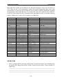
CONTENTS
Lab Session No.
Object
Page No.
Section One: Working with Basic Electronic Components
1
Exploring the electronic components.
2
2a
Familiarization and working with Multimeters.
9
2b
Familiarization and working with Oscilloscope.
15
2c
Familiarization and working with Function Generator.
21
3
Constructing a frequency generator by the use of 555 timer IC.
28
4a
Studying basics behind the construction of a power supply.
32
4b
Constructing a full wave rectifier
38
5
Designing Printed Circuit Boards.
42
6
Demonstrating Printed Circuit Boards.
50
Section Two: Visual Basic Programming
07
Creating first program in Visual Basic.
55
08
Learning the Visual Basic building blocks and develop programs using
62
them.
09
Understanding Controls for Making Choices in Programming
67
10
Understanding Arrays in Visual Basic.
72
11
Performing Mathematical functions in Visual Basic
77
12
Connecting to an Access database using the VB Data Control
79
13
Designing a Simple Stop Watch using VB Timer Control
81
14
Designing Quadratic Function Graph Plotter in VB
83
Section Three: Mathematical Modeling Using MATLAB
15
Starting out with MATLAB
86
16
Solving Linear Algebra Problems (Part I)
94
17
Solving Linear Algebra Problems (Part II)
97
18
Matrix Operations
101
19
Graphical Representation of Mathematical Functions
108
Section Four: Working with HTML
20
Introduction to Internet Basics
115
21
Applying HTML Basic tags
124
22
Applying Lists tags in HTML
130
23
Applying Links and Inserting Images in Webpages with HTML
133
Section One
Working with Basic Electronic
Components
Engineering Workshop
Lab Session 01
NED University of Engineering & Technology – Department of Computer & Information Systems Engineering
Lab Session 01
OBJECT
Exploring the electronic components.
COMPONENTS REQUIRED
Capacitors, Transistors, different Diodes and inductor
THEORY
Conductors
A conductor is any substance that allows an electrical charge to flow easily through it. Metals,
such as copper, are good conductors because their atoms have many electrons (negatively
charged particles) that can readily flow.
Insulators
An insulator is any substance that cannot easily allow a flow of charge. Plastics and ceramics are
good insulators. Electrons in the molecules of these materials are restricted. They cannot readily
form an electric current.
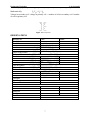
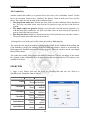
Capacitor
Capacitor is an electrical component used for storing charge, composed of pairs of conducting
plates separated by an insulating material called a dielectric. A potential difference builds up as
charge is stored on the plates, increasing the electric field between them, until it discharges all its
energy in a rapid burst.
Figure 1.1: Capacitor
2
Engineering Workshop
Lab Session 01
NED University of Engineering & Technology – Department of Computer & Information Systems Engineering
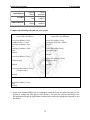
Value
1.5pF
3.3pF
10pF
15pF
20pF
30pF
33pF
47pF
56pF
68pF
75pF
82pF
91pF
100pF
120pF
130pF
150pF
180pF
220pF
330pF
470pF
560pF
680pF
750pF
820pF
Type
Ceramic
Ceramic
Ceramic
Ceramic
Ceramic
Ceramic
Ceramic
Ceramic
Ceramic
Ceramic
Ceramic
Ceramic
Ceramic
Ceramic
Ceramic
Ceramic
Ceramic
Ceramic
Ceramic
Ceramic
Ceramic
Ceramic
Ceramic
Ceramic
Ceramic
Code
.
.
.
.
.
.
.
.
.
.
.
.
.
101
121
131
151
181
221
331
471
561
681
751
821
Value
1,000pF/0.001uF
1,500pF/0.0015uF
2,000pF/0.002uF
2,200pF/0.0022uF
4,700pF/0.0047uF
5,000pF/0.005uF
5,600pF/0.0056uF
6,800pF/0.0068uF
0.01uF
0.015uF
0.02uF
0.022uF
0.033uF
0.047uF
0.05uF
0.056uF
0.068uF
0.1uF
0.2uF
0.22uF
0.33uF
0.47uF
0.56uF
1uF
2uF
Type
Ceramic/Mylar
Ceramic/Mylar
Ceramic/Mylar
Ceramic/Mylar
Ceramic/Mylar
Ceramic/Mylar
Ceramic/Mylar
Ceramic/Mylar
Ceramic/Mylar
Mylar
Mylar
Mylar
Mylar
Mylar
Mylar
Mylar
Mylar
Mylar
Mylar
Mylar
Mylar
Mylar
Mylar
Mylar
Mylar
Code
102
152
202
222
472
502
562
682
102
.
203
223
333
473
503
563
683
104
204
224
334
474
564
105
205
Table 1.1: Capacitor code guide chart
Semiconductors
Some nonmetals, such as silicon, conduct electricity under certain conditions, but are not good
conductors. Because of this, they are classified as semiconductors. In a pure state, they conduct
electricity very poorly and so they are “doped” with impurities to make them better conductors.
Semiconductors are used to make many electronic components.
Doping
The process of modifying the structure of a semi-conducting material such as silicon to enhance
its conducting properties. Doping can involve the addition of atoms with extra electrons to carry
negative charge, or the insertion of electron-deficient atoms, creating “holes” that act as positive
charge carriers.
pn junction
When one n-type semi-conductor and one p-type semi- conductor are placed together, the
resulting device has some very special properties. The region that is formed by adjoining a ptype semiconductor and an n-type semiconductor is called a pn junction.
3
Engineering Workshop
Lab Session 01
NED University of Engineering & Technology – Department of Computer & Information Systems Engineering
Forward Biasing
In order to "forward-bias" the device and decrease the size of the depletion region, one should set
up an electric field such that a positive voltage is in contact with the p-type end of the device and
a negative voltage is in contact with the n-type semi-conductor.
The result of this applied voltage is that the holes in the p-type side of the device and the
electrons in the n-type side of the device are both repelled from the applied voltages and
"pushed" towards the depletion region. This results in a decrease in the width of the depletion
region and, consequently, the energy needed to cross that barrier. This makes is easier for current
to flow and, if the applied voltages are large enough (typically 0.6 V for silicon), the pn-device
will start to conduct freely.
Reverse-Biasing
In order to increase the size of the depletion region and thereby make it tougher for current to
flow one should "reverse-bias" the device. To do this, electric voltages are applied such that a
positive voltage is in contact with the n-type end of the device, and a negative voltage is placed
in contact with the p-type semi-conductor. When this electric field is set up, the positive voltage
will attract the negative electrons from the n-type semiconductor, drawing them away from the
depletion region. Conversely, the negative voltage will attract the positive holes away from the
depletion region. These new forces of attraction result in an enlargement of the depletion region
and, consequently, the energy gap between regions.
Unfortunately, there is a limit to the sensitivity and the amount of external voltage that can be
applied. This voltage is determined by the resistance of the particular semi-conductors. At some
maximum applied voltage, the semi-conductor device will breakdown and will start to conduct
freely.
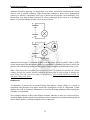
Diodes
A diode is an electronic component that converts alternating current (AC) in an electric circuit to
direct current (DC). Alternating current (which is the type used around the home) travels in one
direction first and then in the opposite direction. Direct current flows in one direction only, and
can be made by batteries. Diodes work by restricting the flow of electrons to one direction only.
Figure 1.2: Circuit Symbol
Figure 1.3: Physical View
How to test a diode
To test a silicon diode such as a 1N914 or a 1N4001, all you need is an ohm-meter. If you are
using an analog VOM type meter, set the meter to one of the lower ohms scale, say 0-2K, and
measure the resistance of the diode both ways. If you get zero both ways, the diode is faulty. If
4
Engineering Workshop
Lab Session 01
NED University of Engineering & Technology – Department of Computer & Information Systems Engineering
you et INFINITY both ways, the diode is faulty again. If you get INFINITY one way and some
reading the other way (the value is not important) then the diode is good.
If you use a digital multi-meter (DMM), then there should be a special setting on the Ohms range
for testing diodes. Often the setting is marked with a diode symbol as figure 1.2.
Measure the diode resistance both ways. One way the meter should indicate an open circuit, the
other way you should get a reading. That indicates the diode is good. If you measure an open
circuit both ways, the diode is open. If you measure low resistance both ways, the diode is
shorted.
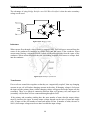
Transistors
A transistor is an electronic semiconductor device in which one electric current controls another
current. It can be used either as an amplifier or a switch. They are made by sandwiching one type
of doped semiconductor between two layers of another type. The three parts that make up a
transistor are the base, the emitter, and the collector. Computers contain millions of transistors
that respond in a few nanoseconds to changes in current. This enables computers to operate
extremely quickly.
Types of Transistors
The most common type of transistor, the junction or bipolar transistor has three electrodes called
the emitter, base, and collector. The input signal voltage is most frequently applied between the
base and the emitter, and the output is taken between the collector and the emitter; since the
emitter is common to both input and output circuits, this is called the common emitter
configuration.
The basic types of transistors are the junction (or bipolar) type, and the field effect transistor
(FET). Both types can be incorporated into integrated circuits.
Junction Transistor
A junction transistor consists of regions of n-type (negative-type) or p-type (positive-type)
material, made by adding an appropriate impurity in a process known as doping. The base must
be of the opposite type of material from that of the other two electrodes, and so both npn and pnp
transistors exist.
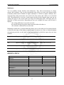
NPN Transistor
The transistor in which a p-type material is sandwiched between two n-type materials is called an
npn transistor.
5
Engineering Workshop
Lab Session 01
NED University of Engineering & Technology – Department of Computer & Information Systems Engineering
Figure 1.4: NPN Transistor
Figure 1.5: PNP Transistor
PNP Transistor
The transistor in which an n-type material is sandwiched between two p-type materials is called a
pnp transistor.
How to test a Transistor for NPN or PNP
If you have a transistor and you do not know if it is PNP or NPN, then you can find it out using
your Ohm-meter if you know which lead of your meter is internally connected to the positive
terminal of the battery inside the meter.
Assuming you know where C, B, and E are on the transistor, do the following. Connect the
positive lead of your Ohm-meter to the base. Touch the other lead of your meter to the collector.
If you get a reading, the transistor is NPN. To verify, move the lead from the collector to the
emitter and you should still get a reading.
If your meter reads open circuit, then connect the negative lead t the base and touch the positive
lead to the collector. If you get a reading, then the transistor is PNP. Verify by measuring from
base to emitter.
Field Effect Transistor (FET)
One type of field effect transistor consists of a narrow channel of n-type material within some ptype material through which current can flow. The channel has an input connection known as the
source and an output connection known as the drain. The size of current that can flow through
the channel is influenced by the voltage on a third connection, known as the gate, that is made to
the p-type material. The gate is so-called, because changing the voltage applied to it makes the
size of the channel narrower, “closing the gate,” and reducing the current that can flow between
the source and the drain. The source corresponds to the emitter of a junction transistor, the drain
to the collector, and the gate to the base. One of the main advantages of FETs is that they can be
made much smaller than junction transistors, so they are widely used in computer chips.
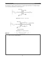
Transformers
A transformer is two coils of wire (called the primary coil and the secondary coil) wrapped
around a piece of iron. It makes AC voltages larger or smaller, depending on how the coils are
arranged. A transformer with more windings in the secondary coil than in the primary increases
voltage and is called a step-up transformer. The reverse arrangement, a step-down transformer,
decreases voltage.
6
Engineering Workshop
Lab Session 01
NED University of Engineering & Technology – Department of Computer & Information Systems Engineering
Mathematically,
Vs /Vp = Ns / Np
Voltage in secondary coil / voltage in primary coil = number of coils in secondary coil / number
of coils in primary coil.
Figure 1.6: Transformer
OBSERVATIONS
Resistors # 1
Band # 1
Band # 2
Multiplier
Tolerance
Total Resistance
Observed Resistance
Resistor # 2
Band # 1
Band # 2
Multiplier
Tolerance
Total Resistance
Observed Resistance
Resistor # 3
Band # 1
Band # 2
Multiplier
Tolerance
Total Resistance
Observed Resistance
Resistor # 4
Band # 1
Band # 2
Multiplier
Tolerance
Total Resistance
Observed Resistance
Color
Value
7
Engineering Workshop
Lab Session 01
NED University of Engineering & Technology – Department of Computer & Information Systems Engineering
Diode
Diode #
Good / Bad
Diode # 1
Diode # 2
Capacitor
Printed Value
Capacitor # 1
Capacitor # 2
Capacitor # 3
Transistor
Transistor #
Type (NPN/PNP)
Transistor # 1
Transistor # 1
RESULT
-
Diodes were checked and found good / bad.
Values of capacitors were verified using Multimeter.
Transistors were checked for NPN / PNP.
8
Engineering Workshop
Lab Session 02(a)
NED University of Engineering & Technology – Department of Computer & Information Systems Engineering
Lab Session 02(a)
OBJECT
Familiarization and working with Multimeters.
COMPONENTS REQUIRED
Variety of Resistors (Variable, Carbon, Wire wound, Fuse-able, Film resistance etc), Digital
multimeter (DMM) or Digital Voltmeter (DVM)
THEORY
Current
A flow of electric charge or the charge flowing per second is called Current (I). It is measured in
Amperes (A) – Electric current is carried either by the flow of negatively charged electrons, or of
positively charged ions, or, in semiconductors, by positive “holes” where electrons are missing
from a crystal structure.
Voltage
People often very loosely speak of the “voltage flowing through” a circuit, but this is both
misleading and incorrect. It is current that flows through a circuit. Voltage is the difference in
potential between two points in a circuit, and as such, it is correct to speak of the voltage across
some component of the circuit or the potential difference between two points. It is the difference
in potential that causes a current to flow.
Potential Difference
The potential difference between points A and B is the work done in bringing a unit charge from
A to B. The work is measured in joules, and the unit of potential difference is the volt. From this
definition, if a charge of Q coulombs is moved through a potential difference of V volts, the work
done, W, in joules, is given by W = QV.
Electromotive Force (E.M.F.)
If a potential difference can be used to drive a current through a circuit, it is known as an
electromotive force (e.m.f.). It is the same as the voltage measured across a source of current
when no current is actually being supplied. E.m.f. is not really a force at all; it is measured in the
same units as voltage (volts).
9
Engineering Workshop
Lab Session 02(a)
NED University of Engineering & Technology – Department of Computer & Information Systems Engineering
Definition of the Volt - A volt is the practical and SI unit of potential difference, voltage, and
electromotive force (e.m.f.). It is named for Alessandro Volta. In the 18th century, he carried out
important experiments on current and how it flows. The potential difference across a conductor
is defined to be 1 volt when 1 joule of work is done to give it a charge of 1 coulomb. Alternative
units of voltage would therefore be joules per coulomb, where 1 J/C = 1 V.
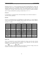
Resistance
It is the hindrance or opposition to flow of electrons through a circuit. Electrical resistance is
measured in ohms (symbol Ω).
Resistors
Resistors are components that are used deliberately to add resistance to a circuit, helping to
control current and protect other components. They are made with a resistive metal, carbon, or
metal that is very thin.
Colour
Black
Brown
Red
Orange
Yellow
Green
Blue
Violet
Grey
White
Silver
Gold
Band 1
0
1
2
3
4
5
6
7
8
9
---
Band 2
0
1
2
3
4
5
6
7
8
9
---
Band 3
0
1
2
3
4
5
6
7
8
9
---
Multiplier
1
10
100
1000
10000
100000
1000000
10000000
100000000
----
Tolerance
1%
2%
5%
10%
Table 2(a).1: Resistor color band chart
Ohm’s Law
Ohm’s law states that for a given electrical conductor the voltage across the ends is directly
proportional to the current flowing the conductor, when temperature and other physical
conditions are kept constant. Ohm‟s law is written as
VI
 V = I×R
where V is the voltage, I is the current, and R is the resistance. The units of voltage, current, and
resistance are the volt (V), ampere (A), and ohm () respectively.
10
Engineering Workshop
Lab Session 02(a)
NED University of Engineering & Technology – Department of Computer & Information Systems Engineering
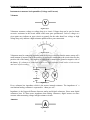
Instruments to measure basic quantities (Voltage and Current)
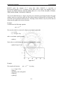
Voltmeter
Figure 2(a).1
Voltmeters measures voltage or voltage drop in a circuit. Voltage drop can be used to locate
excessive resistance in the circuit which could cause poor performance. Lack of voltage at a
given point may indicate an open circuit or ground. On the other hand, low voltage or high
voltage drop, may indicate a high resistance problem like a poor connection.
Figure 2(a).2
Voltmeters must be connected in parallel with the device or circuit so that the meter can tap off a
small amount of current. That is the positive or read lead is connected to the circuit closest to the
positive side of the battery. The negative or black lead is connected to ground or negative side of
the battery. If a voltmeter is connected in series, its high resistance would reduce circuit current
and cause a false reading.
Figure 2(a).3
Every voltmeter has impedance which is the meters internal resistance. The impedance of a
conventional analog voltmeter is expressed in “ohms per volt”.
Impedance is the biggest difference between analog and digital voltmeters. Since most digital
voltmeters have 50 times more impedance than analog voltmeters, digital meters are more
accurate when measuring voltage in high resistance circuits.
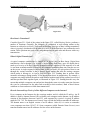
Ammeter:
Figure 2(a).4
11
Engineering Workshop
Lab Session 02(a)
NED University of Engineering & Technology – Department of Computer & Information Systems Engineering
Ammeters measures amperage, or current flow, in a circuit, and provide information on current
draw as well as current continuity. High current flow indicates a short circuit, unintentional
ground or a defective component. Some type of defect has lowered the circuit resistance. Low
current flow may indicate high resistance or a poor connection in the circuit or a discharged
battery. No current indicates an open circuit or loss of power.
Figure 2(a).5
Ammeters must always be connected in series with the circuit, never in parallel. That is, all the
circuit current must flow through the meter. It is connected by attaching the positive lead to the
positive side of the battery/circuit, and the negative lead to negative or ground side of the circuit
Note: These meters have extremely low internal resistance. If connected in parallel, the current
running through the parallel branch created by the meter may be high enough to damage the
meter along with the circuit the meter is connected to. The current should not exceed the
maximum rating of the meter.
Ohmmeters:
An ohmmeter is powered by an internal battery that applies a small voltage to a circuit or
component and measures how much current flow through the circuit or component. It then
displays the result as resistance. Ohmmeters are used for checking continuity and measuring the
resistance of components.
Zero resistance indicate a short while infinite resistance indicates an open in a circuit or device.
A reading higher than the specification indicates a faulty component or a high resistance problem
such as burnt contacts, corroded terminals or loose connection
12
Engineering Workshop
Lab Session 02(a)
NED University of Engineering & Technology – Department of Computer & Information Systems Engineering
Multimeter:
You are probably already familiar with multimeters. They allow measurement of voltage,
current, and resistance. Just as with wristwatches and clocks, in recent years digital meters
(commonly abbreviated to DMM for digital multimeter or DVM for digital voltmeter) have
superseded the analog meters that were used for the first century and a half or so of electrical
work. The multimeters we use have various input jacks that accept „banana‟ plugs, and you can
connect the meter to the circuit under test using two banana-plug leads. The input jacks are
described in Table given below. Depending on how you configure the meter and its leads, it
displays
- the voltage difference between the two leads,
-the current flowing through the meter from one lead to the other, or
- the resistance connected between the leads.
Multimeters usually have a selector knob that allows you to select what is to be measured and to
set the full-scale range of the display to handle inputs of various size. Note: to obtain the highest
measurement precision, set the knob to the lowest setting for which the input does not cause
overflow.
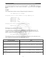
Input jack
Purpose
Limits
COM
reference point used for all measurements
VΩ
input for voltage or resistance measurements
1000 V DC/750 V AC
mA
input for current measurements (low scale)
200 mA
10 A
input for current measurements (high scale)
10A
OBSERVATIONS
Resistors # 1
Band # 1
Band # 2
Multiplier
Tolerance
Total Resistance
Observed Resistance
Resistor # 2
Band # 1
Band # 2
Multiplier
Tolerance
Total Resistance
Color
13
Value
Engineering Workshop
Lab Session 02(a)
NED University of Engineering & Technology – Department of Computer & Information Systems Engineering
Observed Resistance
Resistor # 3
Band # 1
Band # 2
Multiplier
Tolerance
Total Resistance
Observed Resistance
Resistor # 4
Band # 1
Band # 2
Multiplier
Tolerance
Total Resistance
Observed Resistance
RESULT
1.
Values of Resistors were checked using colour code and Multimeter and they were found
approximately same.
2. Volage across circuit is checked by shifting the knob of multimeter to voltage
mesuring dial and found the circuit is properly connected
3. Current drop in the circuit circuit is found and verfied that the circuit is properly
connected with the help of DMM.
14
Engineering Workshop
Lab Session 02(b)
NED University of Engineering & Technology – Department of Computer & Information Systems Engineering
Lab Session 02(b)
OBJECT
Familiarization and working with Oscilloscope.
COMPONENTS REQUIRED
Oscilloscope, Function generator, power supplies
THEORY
With its many switches and knobs, a modern oscilloscope can easily intimidate the faint of heart,
yet the scope is an essential tool for electronics troubleshooting and you must become familiar
with it. Accordingly, the rest of this laboratory session will be devoted to becoming acquainted
with such an instrument and seeing some of the things it can do. The oscilloscope we use is the
Tektronix TDS210 (illustrated in Fig. 2(b).1). If you don‟t have a TDS210, any dual-trace
oscilloscope, analog or digital, can be used for these labs as long as the bandwidth is high
enough – ideally, 30 MHz or higher. While the description below may not correspond exactly to
your scope, with careful study of its manual you should be able to figure out how to use your
scope to carry out these exercises. The TDS210 is not entirely as it appears. In the past you may
have used an oscilloscope that displayed voltage as a function of time on a cathode-ray tube
(CRT). While the TDS210 can perform a similar function, it does not contain a CRT (part of the
reason it is so light and compact).
Figure 2(b).1 Osilloscope Controls
15
Engineering Workshop
Lab Session 02(b)
NED University of Engineering & Technology – Department of Computer & Information Systems Engineering
Until the 1990s, most oscilloscopes were purely „analog‟ devices: an input voltage passed
through an amplifier and was applied to the deflection plates of a CRT to control the position of
the electron beam. The position of the beam was thus a direct analog of the input voltage. In the
past few years, analog scopes have been largely superseded by digital devices such as the
TDS210 (although low-end analog scopes are still in common use for TV repair, etc.). A digital
scope operates on the same principle as a digital music recorder. In a digital scope, the input
signal is sampled, digitized, and stored in memory. The digitized signal can then be displayed on
a computer screen. One of your first objectives will be to set up the scope to do some of the
things for which you may already have used simpler scopes. After that, you can learn about
multiple traces and triggering. In order to have something to look at on the scope, you can use
your breadboard‟s built-in function generator, a device capable of producing square waves,
sinusoidal waves, and triangular waves of adjustable amplitude and frequency. But start by using
the built-in „calibrator‟ signal provided by the scope on a metal contact labeled „probe comp‟ (or
something similar), often located near the lower right-hand corner of the display screen.
Note that a leg folds down from the bottom of the scope near the front face. This adjusts the
viewing angle for greater comfort when you are seated at a workbench, so we recommend that
you use it.
Probes and probe test
Oscilloscopes come with probes: cables that have a coaxial connector (similar to that used for
cable TV) on one end, for connecting to the scope, and a special tip on the other, for connecting
to any desired point in the circuit to be tested. To increase the scope‟s input impedance and affect
the circuit under test as little as possible, we generally use a „10X‟ attenuating probe, which has
circuitry inside that divides the signal voltage by ten. Some scopes sense the nature of the probe
and automatically correct for this factor of ten; others (such as the TDS210) need to be told by
the user what attenuation setting is in use.
As mentioned above, your scope should also have a built-in „calibrator‟ circuit that puts out a
standard square wave you can use to test the probe (see Fig. 2(b).1). The probe‟s coaxial
connector slips over the „CH 1‟ or „CH 2‟ input jack and turns clockwise to lock into place. The
probe tip has a springloaded sheath that slides back, allowing you to grab the calibrator-signal
contact with a metal hook or „grabber‟.
An attenuating scope probe can distort a signal. The manufacturer therefore provides a
„compensation adjustment‟ screw, which needs to be tuned for minimum distortion. The screw is
usually located on the assembly that connects the probe to the scope, or, occasionally, on the tip
assembly.
-
-
Display the calibrator square-wave signal on the scope. If the signal looks distorted (i.e.,
not square), carefully adjust the probe compensation using a small screwdriver. (If you
have trouble achieving a stable display, try „autoset‟.)
Check your other probe. Make sure that both probes work, are properly compensated, and
have equal calibrations. Sketch the observed waveform. (Consult your oscilloscope user
manual for more information about carrying out a probe test.)
16
Engineering Workshop
Lab Session 02(b)
NED University of Engineering & Technology – Department of Computer & Information Systems Engineering
Note that each probe also has an alligator clip (sometimes referred to as the „reference lead‟ or
„ground clip‟). This connects to the shield of the coaxial cable. It is useful for reducing noise
when looking at high-frequency (time intervals of order nanoseconds) or low-voltage signals.
Since it is connected directly to the scope‟s case, which is grounded via the third prong of the
AC power plug, it must never be allowed to touch a point in a circuit other than ground!
Otherwise you will create a short circuit by connecting multiple points to ground, which could
damage circuit components.
This is no trouble if you are measuring a voltage with respect to ground. But if you want to
measure a voltage drop between two points in a circuit, neither of which is at ground, first
observe one point (with the probe) and then the other. The difference between the two
measurements is the voltage across the element. During this process, the reference lead should
remain firmly attached to ground and should not be moved! (Alternatively, you can use two
probes and configure the scope to subtract one input from the other.)
Warning: A short circuit will occur if the probe’s reference lead is connected anywhere other
than ground.
Display
Your oscilloscope user‟s manual will explain the information displayed on the scope‟s screen.
Record the various settings: timebase calibration, vertical scale factors, etc.
Vertical controls
There is a set of „vertical‟ controls for each channel (see Fig. 2(b).1). These adjust the sensitivity
(volts per vertical division on the screen) and offset (the vertical position on the screen that
corresponds to zero volts). The „CH 1 ‟ and „CH 2 ‟ menu buttons can be used to turn the display
of each channel on or off; they also select which control settings are programmed by the pushbuttons just to the right of the screen.
Horizontal sweep
To the right of the vertical controls are the horizontal controls (see Fig. 2(b).1). Normally, the
scope displays voltage on the vertical axis and time on the horizontal axis. The sec/div knob sets
the sensitivity of the horizontal axis, i.e. the interval of time per horizontal division on the screen.
The position knob moves the image horizontally on the screen.
Triggering
Triggering is probably the most complicated function performed by the scope. To create a stable
image of a repetitive waveform, the scope must „trigger‟ its display at a particular voltage,
known as the trigger „threshold‟. The display is synchronized whenever the input signal crosses
that voltage, so that many images of the signal occurring one after another can be superimposed
in the same place on the screen. The level knob sets the threshold voltage for triggering. You can
select whether triggering occurs when the threshold voltage is crossed from below(„rising-edge‟
17
Engineering Workshop
Lab Session 02(b)
NED University of Engineering & Technology – Department of Computer & Information Systems Engineering
triggering) or from above („falling-edge‟ triggering) using the trigger menu (or, for some scope
models, using trigger control knobs and switches). You can also select the signal source for the
triggering circuitry to be channel 1, channel 2, an external trigger signal, or the 120 V AC power
line, and control various other triggering features as well.
Since setting up the trigger can be tricky, the TDS210 provides an automatic setup feature (via
the autoset button) which can lock in on almost any repetitive signal presented at the input and
adjust the voltage sensitivity and offset, the time sensitivity, and the triggering to produce a
stable display.
After getting a stable display of the calibrator signal, adjust the level knob in each direction until
the scope just barely stops triggering.
Next connect the scope probe to the breadboard‟s function generator –you can do this by
inserting a wire into the appropriate breadboard socket and grabbing the other end of the wire
with the scope probe‟s grabber. The function generator‟s amplitude and frequency are adjusted
by means of sliders and slide switches.
Display both scope channels, with one channel looking at the output of the function generator
and the other looking at the scope‟s calibrator signal. Make sure the vertical sensitivity and offset
are adjusted for each channel so that the signal trace is visible.
Additional features
The TDS210 has many more features than the ones we‟ve described so far. Particularly useful
are the digital measurement features. Push the measure button to program these.You can use
them to measure the amplitude, period, and frequency of a signal. The scope does not measure
amplitude directly. How then can you derive the amplitude from something the scope does
measure?
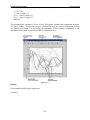
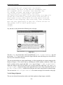
EXERCISE
1.
Explain briefly the various pieces of information displayed around the edges of the screen.
-
________________________________________________________________
________________________________________________________________
________________________________________________________________
________________________________________________________________
________________________________________________________________
________________________________________________________________
________________________________________________________________
________________________________________________________________
________________________________________________________________
_______________________________________________________________
18
Engineering Workshop
Lab Session 02(b)
NED University of Engineering & Technology – Department of Computer & Information Systems Engineering
(The following exercises will give you practice in understanding the various settings. For each,
you should study the description in your oscilloscope user’s manual. The description belowis
specific to the TDS210; if you have a different model, your manual will explain the
corresponding settings for your scope)
2.
Display a waveform from the calibrator on channel 1. What happens when you adjust the
position knob? The volts/div knob?
________________________________________________________________
________________________________________________________________
________________________________________________________________
________________________________________________________________
_______________________________________________________________
3. How many periods of the square wave are you displaying on the screen? How many
divisions are there per period? What time interval corresponds to a horizontal division?
Explain how these observations are consistent with the known period of the calibrator signal.
________________________________________________________________
________________________________________________________________
________________________________________________________________
________________________________________________________________
________________________________________________________________
________________________________________________________________
________________________________________________________________
4. Adjust the sec/div knob to display a larger number of periods. Now what is the time per
division? How many divisions are there per period?
________________________________________________________________
________________________________________________________________
________________________________________________________________
_______________________________________________________________
5. What is the range of trigger level that gives stable triggering on the calibrator signal? How
does it compare with the amplitude of the calibrator waveform? Does this make sense?
Explain.
________________________________________________________________
________________________________________________________________
________________________________________________________________
________________________________________________________________
________________________________________________________________
________________________________________________________________
________________________________________________________________
________________________________________________________________
19
Engineering Workshop
Lab Session 02(b)
NED University of Engineering & Technology – Department of Computer & Information Systems Engineering
________________________________________________________________
________________________________________________________________
________________________________________________________________
________________________________________________________________
_______________________________________________________________
6. Look at each of the waveforms available from the function generator: square, sine, and
triangle. Try out the frequency and voltage controls and explain how they work. Adjust the
function generator‟s frequency to about 1 kHz.
________________________________________________________________
________________________________________________________________
________________________________________________________________
________________________________________________________________
________________________________________________________________
________________________________________________________________
_______________________________________________________________
7. What do you see on the screen if you trigger on channel 1? On channel 2?
________________________________________________________________
________________________________________________________________
________________________________________________________________
________________________________________________________________
8.
What do you see if neither channel causes triggering (for example, if the trigger threshold is
set too high or too low)?
________________________________________________________________
________________________________________________________________
________________________________________________________________
________________________________________________________________
________________________________________________________________
________________________________________________________________
________________________________________________________________
20
Engineering Workshop
Lab Session 02(c)
NED University of Engineering & Technology – Department of Computer & Information Systems Engineering
Lab Session 02(c)
OBJECT
Familiarization and working with Function Generator
COMPONENTS REQUIRED
Oscilloscope, Function Generator FG-8002, Variable power supplies, connecting wires
THEORY
Function generators are among the most important and versatile piece of equipment. In
electronics design and troubleshooting, the circuit under scrutiny often requires a controllable
signal to simulate its normal operation. The testing of physical system and transducers often
needs stable and reliable signals. The signal levels needed range from micro volts to tens of volts
or more.
Modern DDS(Direct Digital Synthesis) function generator are able to prove a wide variety of
signals. Today`s basic units are capable of sine, square and triangle outputs from less than 1 Hz
to at least 1 MHz, with variable amplitude and adjustable DC offset. Many generators include
extra features, such as higher frequency capability, variable symmetry, frequency sweep, AM /
FM operation and gated burst mode. More advance model offer a variety of additional
waveforms and arbitrary waveforms generator can supply user can define periodic waveforms.
Function generators are used where stable and repeatable stimulus signals are needed. Here are
some common use and users.





Research and development
Educational institutions
Electronics and electrical equipment repair businesses
Stimulus/response testing, frequency response characterization, and in-circuit signal
injection
Electronic hobbyists
To use a function generator to its best advantage, the user should have a basic understanding of
the instrument‟s controls, features, and operating modes. This lab session provides useful
information to those with little knowledge of function generator, as well as the experienced
technician or engineer who wishes to refresh his/her memory or explore new uses for function
generators and more sophisticated arbitrary waveform generators.
First, we will explain the controls of a typical function generator. Next we will look at the theory
of how a DDS function generator works. The next section is on controls /applications and
contains the majority of the material in this lab session.
21
Engineering Workshop
Lab Session 02(c)
NED University of Engineering & Technology – Department of Computer & Information Systems Engineering
There are a variety of function generators on the markets spanning the cost range from a few tens
of dollars to tens of thousands of dollars. Some are dedicated instrument (the ones we will look
at in more detail), some are black boxes with USB interfaces and an Output terminal, some are
plugged into computer or instrumentation buses, and some are software programs that run on a
PC to generate waveforms on the parallel port or via a sound card. There are also inexpensive
Kits for hobbyists.
The software-only function generator tends to be the least expensive and can be attractive for
students and hobbyists on a budget. They are also the most limited in frequency capabilities,
often just spanning the audio range.
The black boxes are next in cost and have the advantage of portability and low power. They are
often intended to operate with laptop computers.
Generators that plug into different buses (e.g. PC, VXI) are appropriate where space is at a
premium and a custom measurement system needs to be put together for e.g. a dedicated
purpose.
Dedicated bench top generators are self-Contained with needed control and display. The more
expensive dedicated instruments add features and usually include one or more types of interface
Connection that allow computer control.
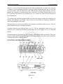
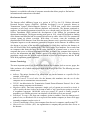
FUNCTION GENERATOR FG-8002
Figure 2(c).1
22
Engineering Workshop
Lab Session 02(c)
NED University of Engineering & Technology – Department of Computer & Information Systems Engineering
FRONT PANEL
1.
POWER Switch
Pressing this push switch turns on power.
2.
POWER Lamp
LED lights up when power is on.
3.
Frequency Dial
This Variable potentiometer varies output frequency within the selected range with the
frequency range selector.
4.
SWEEP WIDTH / PULL ON Control
Pulling the knob selects internal sweep and rotating it controls sweep width. Rotate it
counter clockwise to get a minimum sweep width (1: 1) and rotate it clockwise to get a
maximum sweep width (100:1). To get a maximum sweep width, set the frequency dial
to minimum scale (below 0.2 scales). Pushing the knob selects external sweep, which is
implemented when external sweep voltage is applied to the VCF input connector.
5.
SWEEP RATE Control
This controls weep rate (sweep frequency) of internal sweep oscillator.
6.
SYMMERTRY Control
This controls symmetry (duty cycle) of output signal waveform within range of 10: 1 to
1: 10.
Fig 4.2. Shows waveforms varied by symmetry control.
7.
DC OFFSET Control
The DC offset control can provide up to + 10V open circuit, or + 5V into 50.
Figure 2(c).2
23
Engineering Workshop
Lab Session 02(c)
NED University of Engineering & Technology – Department of Computer & Information Systems Engineering
Clockwise rotation admixes positive voltage and counter clockwise rotation admixes
negative voltage.Ω.
Fig 4.3, shows the various operating conditions encountered when using DC offset.
Figure 2(c).3: DC Offset control
8.
AMPLITUDE/PULL – 20dB Control
Amplitude of output signal can be controlled by this knob. Maximum attenuation is more
than 20dB when the knob is rotated fully counter clockwise. Pulling this knob make
attenuation of 20dB, so the output signal can be attenuated by 40dB when this is pulled
and rotated fully counter clockwise.
9.
FREQUENCY RANGE Selector
Select one of the following seven ranges of oscillation frequency as desired.
10.
FUNCTION Selector
Push one of the three knobs to get a desired waveform out of sine wave, triangle wave
and square wave.
11.
VCF IN Connector
Frequency of output signal can be varied by applying voltage to this connector.
Application of voltage from 0 to + 10V provides frequency variation up to 100: 1. To
maximum variation, set the frequency dial to minimum scale. (below 0.2 scale)
12.
TTL – OUTPUT Connector
TTL – level square waves output from here.
13.
OUTPUT Connector
This is the main output connector for sine wave, triangle wave and square wave selected
with the FUNCTION Selector.
24
Engineering Workshop
Lab Session 02(c)
NED University of Engineering & Technology – Department of Computer & Information Systems Engineering
14.
Voltage Selector
Select rated voltage 110V or 220V according to the power line voltage to be applied to
the instrument.
15.
Power Cord
Connect to a power connector for supplying AC power.
16.
FUSE Holder
Fuse holder for AC power supply. Use a specified fuse for safety of the instrument.
Working with Function Generator
The purpose of this lab is familiarizing you with the basic functions of an oscilloscope and
function generators.
1. Setting Up The Oscilloscope and Function Generator
a. Turn on the oscilloscope with the button on the top. Attach a BNC to alligator cable
to the Channel 1 BNC input connector.
b. On the oscilloscope, set the following controls:
 Channel 1 Volts / Division = 2 (The CH 1 menu button enables/disables the
channel, turn VOLTS/DIV knob).
 Time / Division = 250µs (Turn SECONDS/DIV knob).
 Trigger Source = Channel 1 (Push TRIGGER MENU, select Channel 1 from the
Source menu).
c. Turn on the function generator. Attach another BNC to alligator cable to the output
connector (be careful not to attach it to the Sync (TTL) output). Attach the red
alligator clips from both cables together. Repeat with the black clips.
d. You will now configure the function generator to output a 10Vpp (peak-to-peak), 1
KHz sinusoidal wave.
 Use the output arrows to select the sinusoidal wave pattern.
 Highlight the Frequency option (FREQ under Display/Modify) and use the
MODIFIER and RANGE controls to set an output frequency of 1 KHz.
 Highlight the Amplitude option (AMPL) and adjust Vp (peak voltage) for 5
volts.
e. You should now see a sinusoidal wave on the oscilloscope. If not, then ask a lab
assistant for help. The problem may be with some oscilloscope settings, some
"buried" function generator settings, or the physical connection.
f. Now, make sure the sinusoidal wave is vertically centred on your scope.
 Press the Ch 1 menu button
 Select the Ground option under the Coupling submenu.
 The Channel 1 vertical position should be set to 0.00 divs (0.00V). If it is not,
adjust using the "Vertical Position" knob.
g. Since the cosine wave is the standard for sinusoidal wave patterns, adjust the
horizontal position of the wave so that the positive peak amplitude intercepts the
vertical axis. This can be adjusted using the "Horizontal Position".
25
Engineering Workshop
Lab Session 02(c)
NED University of Engineering & Technology – Department of Computer & Information Systems Engineering
You should now have a stable cosine wave with an amplitude of 5 volts, a phase shift of 0
degrees, and a frequency of 1 KHz (see equation 1) display on the oscilloscope.
h. Using the cursors: The oscilloscopes are equipped with a set of horizontal and vertical
cursors to aid in obtaining measurements. You can use these to measure various
parameters like peak voltage, period, and frequency.
 Measure the Peak-to-Peak amplitude of the waveform using the horizontal
cursors. To do this, press Cursor, and then select Voltage under the Type
submenu. Use the Vertical Position knobs to place the cursors at Vp and Vp. Under the delta submenu the peak to peak voltage will be
recorded. Repeat this process to measure the Peak Voltage.
 Measure both the Period and Frequency of the waveform using the vertical
cursors. To do this, press Cursor, and then select Time under the Type
submenu. Use the Vertical Position knobs to again place the cursors. The
delta submenu displays both the period and frequency measurements.
EXERCISES
1. Perform the same operation as demonstrated in the above exercise using a square wave and
write down you observations along with the waveform you observe on the system
________________________________________________________________
________________________________________________________________
________________________________________________________________
________________________________________________________________
________________________________________________________________
_______________________________________________________________
2. Measure the parameters for the following sinusoidal wave
v(t) = 5 cos(62832t + 0) volts
a. What is the frequency of the waveform in hertz? What is the period? What is Vp?
________________________________________________________________
________________________________________________________________
________________________________________________________________
________________________________________________________________
________________________________________________________________
_______________________________________________________________
b.
Adjust the function generator to output the waveform in equation 2. Start bringing up the
frequency from 1 KHz to the value you calculated in part a, and notice what happens to
the waveform displayed on the oscilloscope. Readjust the sec/div knob on the scope
until one or two periods take up most of the screen. What happens to the signal
displayed on the scope as the frequency from the function generator gets higher?
26
Engineering Workshop
Lab Session 02(c)
NED University of Engineering & Technology – Department of Computer & Information Systems Engineering
________________________________________________________________
________________________________________________________________
________________________________________________________________
________________________________________________________________
________________________________________________________________
________________________________________________________________
________________________________________________________________
________________________________________________________________
________________________________________________________________
_______________________________________________________________
c.
With the cursors, measure Vp (peak) and Vpp (peak-to-peak) and record these values in
your lab book.
________________________________________________________________
________________________________________________________________
________________________________________________________________
________________________________________________________________
________________________________________________________________
________________________________________________________________
_______________________________________________________________
d.
With the cursors, measure the frequency of the waveform and record this value in your
lab book.
________________________________________________________________
________________________________________________________________
________________________________________________________________
________________________________________________________________
________________________________________________________________
________________________________________________________________
e.
Sketch the waveform as best as you can in your lab book. Be sure to fully label your plot
with axes, units and divisions.
27
Engineering Workshop
Lab Session 03
NED University of Engineering & Technology – Department of Computer & Information Systems Engineering
Lab Session 03
OBJECT
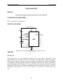
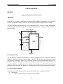
Constructing a frequency generator by the use of 555 timer IC.
COMPONENTS REQUIRED
555 IC, Oscilloscope, Bread board
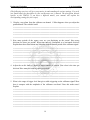
CIRCUIT DIAGRAM
VCC 5V To +15V
R1
8
1
4
8
V (output)
R2
OUT
3
6
555
2
+
C
1
Figure 3.1: Circuit diagram of frequency generator using 555 timer IC
THEORY
555 Timer IC
The 555 timer IC was first introduced around 1971 by the Signetic Corporation as the
SE555/NE555 and was called “the IC time machine”. This timer uses a maze of transistors,
diodes, and the resistors. The 555 comes in two packages, either the round metal can called the
“T Packager” or the more familiar 8-pin Div „V‟ package. Inside the IC, are the resistors and 3
diodes depending on the manufacturer. The equivalent circuit providing the functions of control,
triggering, level sensing or comparison, discharge and power output. Some features of 555 IC
are: Supply voltage between 4.5 and 18 volts, supply 3 to 6 mA and rise and fall time of 100
msec.
28
Engineering Workshop
Lab Session 03
NED University of Engineering & Technology – Department of Computer & Information Systems Engineering
Functions of Different Pins
Pin 1 (Ground) - The ground or common pin is the most –ve supply potential of the device,
which is normally connected to circuit common when operated from the supply voltage.
Pin 2 (Trigger) - It is the input to the lower comparator and is used to set the latch, which in turn
causes the output to go high. This is the beginning of the timing sequence in monostable
operation. Triggering is accomplished by taking the pin from above to below a volt level of 1/3
Volts. The action of the trigger input level sensitive, allowing slow rate of change wave forms, as
well as pulse to be used as trigger sources. The minimum allowable pulse width for triggering is
some what dependent upon pulse level but in general if it is greater than 1 μsec, triggering will
be reliable.
Pin 3 (Output) - The output of the 555 timer comes from a high current to totem-pole. Stage
made up of transistors. The state of the output pin will always reflect the inverse of the logic
state of the latch and this may be seen. Since the latch itself is not directly accessible, this
relationship may be explained in terms of latch input trigger conditions. To trigger the output to a
hi9gh condition the trigger input is taken from a higher to a lower level. This causes the latch to
be set and the output to go high. Activation of the lower comparator is the only manner in which
the output can be placed in the high place (state). This output can be returned to a low state by
causing the threshold to go from a lower to a higher level, which rests the latch. The output can
also be made to go low by taking the reset to a low state near ground.
Pin 4 (Reset) - It is also used to reset the latch and return the output to a low state. The reset
voltage threshold level is 0.7 volts & a sink current of 0.1 mA from this pin is required to reset
the device. These levels are relatively independent of operation Vt level, thus the reset input is
TTL compatible for any supply voltage. The reset input is an overriding function, that is it will
force the output to low state regardless of the state of either of the other inputs. It may thus be
used to terminates an output pulse prematurely to gate oscillations from “on” and “off” etc.
Pin 5 (Control Voltage) - This pin allows accessible to the 2/3 Vt voltage divider pint, the
reference level for the upper comparator. It allows indirect access to the lower comparator, from
the point to the lower comparator input. Use of this terminal is the option of the flexibility by
permitting modification of the tuning period.
When the 555 timer is used in a voltage controlled mode, it voltage controlled operation ranges
from about 1 Volt less than Vt down to within 2 Volts of ground voltages can be safely applied
outside these limits, but they should be confined within the limits of Vt and ground for reliability.
Pin 6 (Threshold) - Pin 6 is one of the input to the upper comparator and is used to reset the
latch, which causes the output to go low.
Resetting via the terminal is accomplished by taking the terminal from below to above a voltage
level of 2/3 Vt. The action of the threshold pin is level sensitive, allowing slow rate of change of
wave-forms. The voltage range that can be safely applied to the threshold, termed the threshold
29
Engineering Workshop
Lab Session 03
NED University of Engineering & Technology – Department of Computer & Information Systems Engineering
current, must also flow into this terminal from the external circuit. This current is typically 100
nA and will define the upper limit of total resistance allowable from pin “6” to Vc.
Pin 7 (Discharge) - This pin is the open collected of npn transistor, the emitter of which goes to
ground. The conduction state of this transistor is identical in tuning to that of the output stage. It
is “on” when the output is low and “off” when the output is high. Maximum collector current is
internally designed, these by removing restriction on capacitor site due to peak pulse-current
discharge. In certain applications, this open collector output can be used as an auxiliary output
terminal, with current sinking capability similar to the output.
Pin 8 (Vt or Vcc) - The Vt pin (also referred to as Vcc) is the positive supply voltage terminal of
555 timer IC. Supply voltage operating range for the 555 is +4.5 Volts (min) to +16 Volts (max)
and it is specified for operation between +5 Volts and +15 Volts. The device will operate
essentially the same over this range of voltages without change in time period. Actually, the most
significant operation capability, which increases for both current and voltage range as the supply
voltage is increased, the supply voltage is increased sensitivity of time interval to supply voltage
change is low, typically 0.1% per Volt.
Types of Waves
Mechanical Waves - The waves which require medium for propagation are called mechanical
waves.
Electromagnetic Waves - The waves that do not require medium for propagation are called
electromagnetic waves. These waves can pass through vacuum.
Matter Waves - These waves are associated with the moving particles, when a very light particle
move with a very high velocity approaching the speed of light.
Travelling Waves - The waves advancing in a medium with a definite velocity are called
travelling waves.
Transverse Waves - The waves in which particles of the medium vibrate perpendicularly to the
direction of propagation of waves are called transverse waves.
Compressional Waves - The waves in which the particles of the medium vibrate along the
direction of the propagation of waves are called compressional or longitudinal waves.
Sinusoidal Waves - The waves whose displacement varies with the sine of phase angle, it is
maximum at 90o in one direction and at 180o in other direction and zero at 0o and 360o are called
sinusoidal waves.
Coherent Waves - Two waves having same wavelength (λ), same frequency (υ), same
amplitude(y) same time period (T) and same phase (φ) producing the crests and troughs at the
same time are called coherent waves.
30
Engineering Workshop
Lab Session 03
NED University of Engineering & Technology – Department of Computer & Information Systems Engineering
Standing Waves - When two waves having same frequency and amplitude propagate with the
same speed in a medium in opposite direction, due to the superposition they vibrate in loops
producing standing waves.
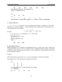
Relation of 555 Timer IC
The frequency, f which is generated is given by:
f =
1.44
(R1 + 2R2) C
OBSERVATIONS & CALCULATIONS
C
R1
R2
Calculated Frequency
Observed Frequency
1
2
3
RESULT
1. Time period of 555 timer can be changed by varying values of resistors and
capacitor.
2. There is a minor change in the calculated and observed frequency for a given
resistor and capacitor.
31
Engineering Workshop
Lab Session 04(a)
NED University of Engineering & Technology – Department of Computer & Information Systems Engineering
Lab Session 04(a)
OBJECT
Studying basics behind the construction of a power supply.
THEORY
Current
A flow of electric charge or the charge flowing per second is called Current (I). It is measured in
Amperes (A) – Electric current is carried either by the flow of negatively charged electrons, or of
positively charged ions, or, in semiconductors, by positive holes where electrons are missing
from a crystal structure.
Types of Current
There are two types of current.
1. Direct Current (called DC)
2. Alternating Current (called AC)
Direct Current
A direct current (DC) is a steady electric current (stream of electrons) flowing in one direction,
as opposed to an alternating current, which reverses direction periodically. Direct current is
produced by simple batteries in cassette players, flashlights, and toys. The main applications of
direct current are in the fields of electronics, traction (battery-powered vehicles and some electric
trains), and electrochemical processing. Alternating current in the form of mains electricity is
often converted into direct current inside electrical appliances, particularly if they contain
electronic components.
Alternating Current
An alternating current (AC) regularly reverses its direction – the electrons that make up the
current constantly change their direction of movement. Alternating current is used almost
universally in mains electricity supplies, in which it reverses direction with a set frequency (for
example, mains electricity in Europe and Asia, including Pakistan has a frequency of 50 Hz,
while in Canada and the United States, it has a frequency of 60 Hz). Its advantage over direct
current is that the voltage may be easily increased (“stepped up”) or decreased (“stepped down)”
using a transformer according to need. High voltages are used to generate and transmit electricity
to our homes, because this helps to reduce the energy lost in the process.
PN junction
When one n-type semiconductor and one p-type semiconductor are placed together, the resulting
device has some very special properties. The region that is formed by adjoining a p-type
semiconductor and an n-type semiconductor is called a pn junction.
32
Engineering Workshop
Lab Session 04(a)
NED University of Engineering & Technology – Department of Computer & Information Systems Engineering
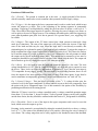
Rectifiers
There are three types of rectifiers namely, half wave rectifier, full wave rectifier and bridge
rectifier. The rectifier user for this power supply is bridge rectifier.
Bridge Rectifier
D2
D1
D3
D4
Figure 4.1: Bridge Rectifier
Figure 4(a).1: Bridge rectifier
The bridge rectifier is similar to a full-wave rectifier because it produces a full-wave output
voltage. Diodes D1 and D3 conduct on the positive half cycle, and D3 and D4 conduct on
negative half cycle. As a result, the rectifed load current flows during both half cycles. During
both half cycles, the load voltage has the same polarity and the load current is in the same
direction. The circuit has changed the A.C. input voltgae to the plulsating D.C. output voltage.
The advantage of using Bridge Recitifer over Full-Wave Rectifieir is that the entire secondary
voltage can be used.
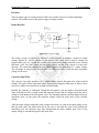
Capacitor Input Filter
The capacitor input filter produces a D.C. output voltage equal to the peak value of the rectified
voltage. This type of filter is the most widely used in power supplies. Other type of filter is choke
input filter which is not used due to its high cost and weight.
Initially, the capacitor is uncharged. During the first quarter cycle the diode is forward biased.
Since it ideally acts like a closed switch the capacitor charges and its voltage equals the source
voltage at each instant of the first quarter cycle. The charging continues until the input reaches its
maximum value. At this point, the capacitor voltage equals the peak value of the rectified
voltage.
After the input voltage reaches the peak, it starts to decrease. As soon as the input voltage is less
then the peak value, the diode turns off. In this case, it acts like the open switch. During the
remaining cycle, the capacitor stays fully charged and the diode remains open. This is why
output voltage is constant and equal to the peak value.
33
Engineering Workshop
Lab Session 04(a)
NED University of Engineering & Technology – Department of Computer & Information Systems Engineering
Figure 4(a).2: Capacitor input filter
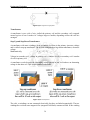
Transformers
A transformer is two coils of wire (called the primary coil and the secondary coil) wrapped
around a piece of iron. It makes AC voltages larger or smaller, depending on how the coils are
arranged.
Step-Up and Step-Down Transformers
A transformer with more windings in the secondary coil than in the primary increases voltage
and is called a step-up transformer. The reverse arrangement, a step-down transformer, decreases
voltage.
Mathematically,
Vs /Vp = Ns / Np
Voltage in secondary coil / voltage in primary coil = number of coils in secondary coil / number
of coils in primary coil.
A transformer works because the alternating voltage carried in one coil induces an alternating
voltage in the other coil. This is called mutual inductance.
Figure 4(a).3: Transformer
The coils, or windings, are not connected electrically, but they are linked magnetically. The two
windings have at least some magnetic flux (magnetic field lines) common to both. If one winding
34
Engineering Workshop
Lab Session 04(a)
NED University of Engineering & Technology – Department of Computer & Information Systems Engineering
(the primary) is connected to an AC supply, the current produces an alternating magnetic flux in
the core which induces an electromotive force (emf) in the other winding (the secondary).
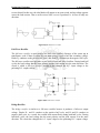
Regulating ICs
Regulating ICs consist of Zener Diodes, which have fixed output voltage even though the current
through it changes. The Zener Diode is got to be reverse biased for normal operation.
Figure 4(a).4: Regulating IC
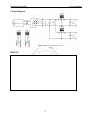
Working
The circuit functions in the following steps:
1. Stepping Down of A.C. Signal
2. Rectification
3. Filtration
4. Regulation
1. Stepping Down of A.C. Signal
The power supply is connected with an A.C. source of 220 V. The current is allowed to flow to
the step-down transformer via the on-off switch and a 2 A fuse. The transformer changes the 220
V signal at input into a 14 V signal at output. The transformer works on the principal of mutual
inductance. According to which, if two coils are wound close together so that they are
„magnetically coupled‟, then any changing currents in one coil will induce changing currents in
the other. If changing voltage is fed across the input coil (the primary) then a similar changing
voltage will appear across the output coil (the secondary). There is no physical connection
between input coil (primary coil) and output coil (secondary coil) but these coils are connected
with magnetic field. The coil with the most turns corresponds to the higher voltage in the
transformer. To step down from a high voltage to a lower one, the primary coil must have more
windings than the secondary.
2. Rectification
The current is then allowed to pass through the bridge-rectifier (made by using four 1N4001
diodes). The diode bridge rectifies the A.C. signal into a pulsating D.C. form. During the positive
half cycle diodes D1 and D3 conducts the current in the positive direction while during the
negative half cycle the gets reverse biased and hence stops the flow of current. On the other hand
diodes D2 and D4 conducts during the negative half cycle. This pulsating D.C. is then allowed to
pass through the capacitor for filtration.
35
Engineering Workshop
Lab Session 04(a)
NED University of Engineering & Technology – Department of Computer & Information Systems Engineering
3. Filtration
The pulsating D.C. is filtered by using a 2200 µF-35V capacitor (to make it more manageable for
the regulator) and thus we get a pure D.C. During the first quarter cycle the rising voltage
charges the capacitor and when the voltage starts to reduce the capacitor starts to discharge and
thus a stabilized D.C. voltage is obtained.
Although the D.C. obtained is almost a pure one, but it may contain some ripples. Thus one more
capacitor (of 0.1 F) is used. This capacitor further filters the D.C. voltage and thus a pure D.C.
is obtained. This pure D.C. is then fed to the regulating ICs of Model 7812 and 7805.
4. Regulation
The regulators have fixed outputs i.e. output of Regulator 7812 is +12 V whereas that of
Regulator 7805 is +5 V. The output obtained from these regulating ICs may contain some ripples
therefore, these outputs are further filtered by using capacitors of 100 F - 25 V and 100 F - 16
V respectively.
EXERCISES
Construct a power supply with two D.C. outputs i.e. 12 Volts and 5 Volts.
Components Required
Component
Transformer - Input 220 V
Output 14 V, 2A
Diode - Model: IN4001
Capacitor - 2200 F, 35 V
Capacitor - 0.1 F/104 pF
Capacitor - 100 F, 25 V
Capacitor - 100 F, 16 V
Regulator - 7812 (for 12 V output)
Regulator - 7815 (for 5 V output)
Bread Board
Banana Jacks
Fuse Holder
Fuse 220 V, 2 A
On – Off Switch with Indicator
Plug, Cord & Casing
Quantity
1
4
1
1
1
1
1
1
1
2 Sets (2 Black & 2 Red)
1
1
1
1
36
Engineering Workshop
Lab Session 04(a)
NED University of Engineering & Technology – Department of Computer & Information Systems Engineering
Circuit Diagram
D2
D1
D3
D4
Figure 4.5: Circuit diagram of a regulating IC
Figure 4(a).5: Circuit Diagram for Power
Supply
RESULT
37
Engineering Workshop
Lab Session 04(b)
NED University of Engineering & Technology – Department of Computer & Information Systems Engineering
Lab Session 04(b)
OBJECT
Constructing a full wave rectifier
COMPONENTS REQUIRED
Multimeter, diodes, capacitor, transformer, bread board
THEORY
PN Junction Diode
If donor impurities are introduced into one side and acceptor impurities into the other side of a
single crystal of semiconductor as shown in figure 4(b).1, a PN junction is formed. It is also
called a diode.
Figure 4(b).1: PN junction in a diode
Capacitance
A capacitor stores electric charge. It consists of a pair of plates set very close to each other but
separated by an insulator layer. When voltage is applied across a capacitor, it stores charge. If
batteries are now removed, the charge remains trapped in the capacitor. This trapped charge is
called capacitance. Capacitance is measured in Farad (F). capacitors are used in different values
like, pico farad (pF), Nano farad (nF), micro farad (F), etc.
Micro farad, F = 10-6 F
Nano farad, nF = 10-9 F
Pico farad, pF = 10-12 F
Rectifiers
Half-Wave Rectifier
The AC source produces a sinusoidal voltage. Assuming an ideal diode, the positive half cycle of
source voltage will forward-bias the diode. Since the switch is closed, the positive half cycle of
source voltage will appear across the load resistor. On the negative half cycle, the diode is
38
Engineering Workshop
Lab Session 04(b)
NED University of Engineering & Technology – Department of Computer & Information Systems Engineering
reverse-biased. In this case, the ideal diode will appear as an open switch, and no voltage appears
across the load resistor. Thus a unidirectional load current is produced i.e. it flows in only one
direction.
Figure 4(b).2: Half wave rectifier
Full-Wave Rectifier
The full-wave rectifier is equivalent to two half-wave rectifiers. Because of the centre tap in
transformer, each of these rectifiers has an input voltage equal to half the secondary voltage.
Diode D1 conducts on the positive half cycle, and diode D2 conducts on the negative half cycle.
The full-wave rectifier acts the same as two back-to-back half-wave rectifiers. During both half
cycles, the load voltage has the same polarity and the load current is in the same direction. The
circuit is called a full-wave rectifier because it has changed the A.C. input voltage to the
pulsating D.C. output voltage.
Figure 6.2: Half wave rectifier
igure 6.2: Half wave rectifier
Figure 4(b).3: Full wave rectifier
Bridge Rectifier
The bridge rectifier is similar to a full-wave rectifier because it produces a full-wave output
voltage. Diodes D1 and D3 conduct on the positive half cycle, and D3 and D4 conduct on
negative half cycle. As a result, the rectifed load current flows during both half cycles. During
both half cycles, the load voltage has the same polarity and the load current is in the same
direction. The circuit has changed the A.C. input voltgae to the plulsating D.C. output voltage.
39
Engineering Workshop
Lab Session 04(b)
NED University of Engineering & Technology – Department of Computer & Information Systems Engineering
The advantage of using Bridge Recitifer over Full-Wave Rectifieir is that the entire secondary
voltage can be used.
D1
D4
220
Vin
Vout
D2
D3
Figure 4(b).4: Bridge rectifier
Inductance
When current flow through a wire it creates a magnetic field. This field grows outward from the
center of the conductor as increases or collapse back into the center of the conductor. When
current starts flowing, a magnetic field is created which grows outwards from the center of the
conductor. When current decreases then the surrounding magnetic field starts to collapse back
into the conductor.
Figure 4(b).5: Principle of induction
Transformers
If two coils are wound close together so that they are „magnetically coupled‟, then any changing
currents in one coil will induce changing currents in the other. If changing voltage is fed across
the input coil (the primary) then a similar changing voltage will appear across the output coil (the
secondary) There is no physical connection between input coil (primary coil) and output coil
(secondary coil) but these coil are connected through magnetic field.
If the primary and secondary winding have the same number of turns, then the output voltage
must be similar to the input. It means output voltage depends on the ratio of input and output
coils. If input coil has 100 number of turns and output coil has 10 number of turns, the ratio is
100/10, then output voltage must be ten time less than the input voltage.
40
Engineering Workshop
Lab Session 04(b)
NED University of Engineering & Technology – Department of Computer & Information Systems Engineering
The transformer, which is shown in figure 6.6 is single output transformer. For multiple outputs
we use centre tape transformer as show in figure 6.7.
Figure 4(b).6: Transformer – Single output
Figure 4(b).7: Center tapped transformer
RESULT
1. Draw a full wave output diagram.
41
Engineering Workshop
Lab Session 05
NED University of Engineering & Technology – Department of Computer & Information Systems Engineering
Lab Session 05
OBJECT
Designing Printed Circuit Boards.
THEORY
You've designed your circuit, perhaps even bread boarded a working prototype, and now it's time
to turn it into a nice Printed Circuit Board (PCB) design. For some designers, the PCB design
will be a natural and easy extension of the design process. But for many others the process of
designing and laying out a PCB can be a very daunting task. There are even very experienced
circuit designers who know very little about PCB design, and as such leave it up to the "expert"
specialist PCB designers. Many companies even have their own dedicated PCB design
departments. This is not surprising, considering that it often takes a great deal of knowledge and
talent to position hundreds of components and thousands of tracks into an intricate (some say
artistic) design that meets a whole host of physical and electrical requirements. Proper PCB
design is very often an integral part of a design. In many designs (high speed digital, low level
analog and RF to name a few) the PCB layout may make or break the operation and electrical
performance of the design. It must be remembered that PCB traces have resistance, inductance,
and capacitance, just like your circuit does.
Back in the pre-computer CAD days, PCBs were designed and laid out by hand using adhesive
tapes and pads on clear drafting film. Many hours were spent slouched over a fluorescent light
box, cutting, placing, ripping up, and routing tracks by hand. Bishop Graphics, Letraset, and
even Dalo pens will be names that evoke fond or not so fond memories. Those days are well and
truly gone, with computer based PCB design having replaced this method completely in both
hobbyist and professional electronics. Computer based CAD programs allow the utmost in
flexibility in board design and editing over the traditional techniques. What used to take hours
can now be done in seconds.
The steps involved in PCB design can be listed here as under:
The Schematic
Before begin to lay out your PCB, you MUST have a complete and accurate schematic diagram.
A PCB design is a manufactured version of your schematic, so it is natural for the PCB design to
be influenced by the original schematic. If your schematic is neat, logical and clearly laid out,
then it really does make your PCB design job a lot easier. Good practice will have signals
flowing from inputs at the left to outputs on the right. With electrically important sections drawn
correctly, the way the designer would like them to be laid out on the PCB. Like putting bypass
capacitors next to the component they are meant for. Little notes on the schematic that aid in the
layout are very useful. For instance, “this pin requires a guard track to signal ground”, makes it
clear to the person laying out the board what precautions must be taken. Even if it is you who
42
Engineering Workshop
Lab Session 05
NED University of Engineering & Technology – Department of Computer & Information Systems Engineering
designed the circuit and drew the schematic, notes not only remind yourself when it comes to
laying out the board, but they are useful for people reviewing the design. Your schematic really
should be drawn with the PCB design in mind.
The schematics for PCB Design can be drawn with the help of available design aid software. The
softwares that are mainly used for this purpose are orcad and workbench. You also learn in
preceding lab session, how to design circuits with the help of these softwares.
Imperial and Metric
As any long time PCB designer will tell you, you should always use imperial units (i.e. inches)
when designing PCBs. This isn‟t just for the sake of nostalgia, although that is a major reason!
The majority of electronic components were (and still are) manufactured with imperial pin
spacing. So this is no time to get stubborn and refuse to use anything but metric units, metric will
make laying out of your board a lot harder and a lot messier.
Some PCB designers will tell you not to use metric millimeters for ANYTHING to do with a
PCB design. In the practical world though, you‟ll have to use both imperial inches (thous) and
the metric millimeter (mm). So which units do you use for what? As a general rule, use thous for
tracks, pads, spacings and grids, which are most of your basic “design and layout” requirements.
Only use mm for “mechanical and manufacturing” type requirements like hole sizes and board
dimensions.
Working to Grids
The second major rule of PCB design, and the one most often missed by beginners, is to lay out
your board on a fixed grid. This is called a “snap grid”, as your cursor, components and tracks
will “snap” into fixed grid positions. Not just any size grid mind you, but a fairly coarse one. 100
thou is a standard placement grid for very basic through hole work, with 50 thou being a standard
for general tracking work, like running tracks between through hole pads. For even finer work
you may use a 25 thou snap grid or even lower. Many designers will argue over the merits of a
20 thou grid v/s a 25 thou grid for instance. In practice, 25 thou is often more useful as it allows
you to go exactly half way between 50 thou spaced pads.
Why is a coarse snap grid so important? It‟s important because it will keep your components neat
and symmetrical; aesthetically pleasing if you may. It‟s not just for aesthetics though - it makes
future editing, dragging, movement and alignment of your tracks, components and blocks of
components easier as your layout grows in size and complexity.
A bad and amateurish PCB design is instantly recognizable, as many of the tracks will not line
up exactly in the center of pads. Little bits of tracks will be “tacked” on to fill in gaps etc. This is
the result of not using a snap grid effectively.
43
Engineering Workshop
Lab Session 05
NED University of Engineering & Technology – Department of Computer & Information Systems Engineering
Good PCB layout practice would involve you starting out with a coarse grid like 50 thou and
using a progressively finer snap grid if your design becomes “tight” on space. Drop to 25 thou
and 10 thou for finer routing and placement when needed. This will do 99% of boards. Make
sure the finer grid you choose is a nice even division of your standard 100 thou.
PCB design is always done looking from the top of your board, looking through the various
layers as if they were transparent. This is how all the PCB packages work. The only time you
will look at your board from the bottom is for manufacturing or checking purposes.
Tracks
There is no recommended standard for track sizes. What size track you use will depend upon (in
order of importance) the electrical requirements of the design, the routing space and clearance
you have available, and your own personal preference. Every design will have a different set of
electrical requirements which can vary between tracks on the board. All but basic non-critical
designs will require a mixture of track sizes. As a general rule though, the bigger the track width,
the better. Bigger tracks have lower DC resistance, lower inductance, can be easier and cheaper
for the manufacturer to etch, and are easier to inspect and rework.
The lower limit of your track width will depend upon the “track/space” resolution that your PCB
manufacturer is capable of. For example, a manufacturer may quote a 10/8 track/space figure.
This means that tracks can be no less than 10 thou wide, and the spacing between tracks (or pads,
or any part of the copper) can be no less than 8 though. The figures are almost always quoted in
thou‟s, with track width first and then spacing.
Real world typical figures are 10/10 and 8/8 for basic boards. The IPC standard recommends 4
thou as being a lower limit. Once you get to 6thou tracks and below though, you are getting into
the serious end of the business and you should be consulting your board manufacturer first. The
lower the track/space figure, the greater care the manufacturer has to take when aligning and
etching the board. They will pass this cost onto you, so make sure that you don‟t go any lower
than you need to. As a guide, with “home made” PCB manufacturing processes like laser printed
transparencies and pre-coated photo resist boards, it is possible to easily get 10/10 and even 8/8
spacing.
Changing your track from large to small and then back to large again is known as “necking”, or
“necking down”. This is often required when you have to go between IC or component pads.
This allows you to have nice big low impedance tracks, but still have the flexibility to route
between tight spots.
44
Engineering Workshop
Lab Session 05
NED University of Engineering & Technology – Department of Computer & Information Systems Engineering
Figure 5.1: Tracks and pads
The thickness of the copper on the PCB is nominally specified in ounces per square foot, with
1oz copper being the most common. You can order other thicknesses like 0.5oz, 2oz and 4oz.
The thicker copper layers are useful for high current, high reliability designs.
Pads
Pad sizes, shapes and dimensions will depend not only upon the component you are using, but
also the manufacturing process used to assemble the board, among other things. There are a
whole slew of standards and theories behind pad sizes and layouts, and this will be explained
later. Suffice it to say at this stage that your PCB package should come with a set of basic
component libraries that will get you started. For all but the simplest boards though, you‟ll have
to modify these basic components to suit your purpose. Over time you will build up your own
library of components suitable for various requirements.
There is an important parameter known as the pad/hole ratio. This is the ratio of the pad size to
the hole size. Each manufacturer will have his own minimum specification for this. As a simple
rule of thumb, the pad should be at least 1.8 times the diameter of the hole, or at least 0.5mm
larger. This is to allow for alignment tolerances on the drill and the artwork on top and bottom
45
Engineering Workshop
Lab Session 05
NED University of Engineering & Technology – Department of Computer & Information Systems Engineering
layers. This ratio gets more important the smaller the pad and hole become, and is particularly
relevant to vias.
There are some common practices used when it comes to generic component pads. Pads for
leaded components like resistors, capacitors and diodes should be round, with around 70 thou
diameter being common. Dual In Line (DIL) components like IC‟s are better suited with oval
shaped pads (60 thou high by 90-100 thou wide is common). Pin 1 of the chip should always be a
different pad shape, usually rectangular, and with the same dimensions as the other pins.
Most surface mount components use rectangular pads, although surface mount SO package ICs
should use oval pads. Again, with pin 1 being rectangular. Other components that rely on pin
numbering, like connectors and SIP resistor packs, should also follow the “rectangular pin 1”
rule. Octagonal pads are seldom used, and should generally be avoided. As a general rule, use
circular or oval pads unless you need to use rectangular.
Vias
Vias connect the tracks from one side of your board to another, by way of a hole in your board.
On all but cheap home made and low end commercial prototypes, vias are made with electrically
plated holes, called Plated Through Holes (PTH). Plated through holes allow electrical
connection between different layers on your board.
What is the difference between a via and a pad? Practically speaking there is no real difference,
they are both just electrically plated holes. But there are differences when it comes to PCB
design packages. Pads and Vias are, and should be, treated differently. You can globally edit
them separately, and do some more advanced things to be discussed later. So don‟t use a pad in
place of a via, and vice-versa.
Holes in vias are usually a fair bit smaller than component pads, with 0.5-0.7mm being typical.
Using a via to connect two layers is commonly called “stitching”, as you are effectively
electrically stitching both layers together, like threading a needle back and forth through
material.
Polygons
“Polygons” are available on many PCB packages. A polygon automatically fills in (or “floods”)
a desired area with copper, which “flows” around other pads and tracks. They are very useful for
laying down ground planes. Make sure you place polygons after you have placed all of your
tacks and pads. Polygon can either be “solid” fills of copper, or “hatched” copper tracks in a
crisscross fashion. Solid fills are preferred, hatched fills are basically a thing of the past.
46
Engineering Workshop
Lab Session 05
NED University of Engineering & Technology – Department of Computer & Information Systems Engineering
Figure 5.2
Clearances
Electrical clearances are an important requirement for all boards. Too tight a clearance between
tracks and pads may lead to “hairline” shorts and other etching problems during the
manufacturing process. These can be very hard to fault find once your board is assembled.
Once again, don‟t “push the limits” of your manufacturer unless you have to, stay above their
recommended minimum spacing if at all possible. At least 15 thou is a good clearance limit for
basic through hole designs, with 10 thou or 8 thou being used for more dense surface mount
layouts. If you go below this, it‟s a good idea to consult with your PCB manufacturer first.
For 240V mains on PCB‟s there are various legal requirements, and you‟ll need to consult the
relevant standards if you are doing this sort of work. As a rule of thumb, an absolute minimum of
8mm (315 thou) spacing should be allowed between 240V tracks and isolated signal tracks.
Good design practice would dictate that you would have much larger clearances than this
anyway.
For non-mains voltages, the IPC standard has a set of tables that define the clearance required for
various voltages. A simplified table is shown here. The clearance will vary depending on
whether the tracks are on an internal layers or the external surface. They also vary with the
operational height of the board above sea level, due to the thinning of the atmosphere at high
altitudes. Conformal coating also improves these figures for a given clearance, and this is often
used on military spec PCBs.
47
Engineering Workshop
Lab Session 05
NED University of Engineering & Technology – Department of Computer & Information Systems Engineering
EXERCISES
1. How you can differ PCB designing from other assembling projects?
__________________________________________________________________
__________________________________________________________________
__________________________________________________________________
__________________________________________________________________
__________________________________________________________________
2. What sort of unit system is preffered in PCB designing, Imperial or Metric? What do you
understand by the term “thou”?
__________________________________________________________________
__________________________________________________________________
__________________________________________________________________
__________________________________________________________________
__________________________________________________________________
3. What are tracks? What is the IPC`s minimum limit for a track?
__________________________________________________________________
__________________________________________________________________
__________________________________________________________________
__________________________________________________________________
__________________________________________________________________
4. Discuss briefly the concept of “necking”
48
Engineering Workshop
Lab Session 05
NED University of Engineering & Technology – Department of Computer & Information Systems Engineering
__________________________________________________________________
__________________________________________________________________
__________________________________________________________________
__________________________________________________________________
__________________________________________________________________
5. What are Vias? How they help connecting two different layers? Is there any difference
between vias and pads?
__________________________________________________________________
__________________________________________________________________
__________________________________________________________________
__________________________________________________________________
__________________________________________________________________
6. Define pad/hole ratio
__________________________________________________________________
__________________________________________________________________
__________________________________________________________________
__________________________________________________________________
__________________________________________________________________
7. What are polygons?
__________________________________________________________________
__________________________________________________________________
__________________________________________________________________
__________________________________________________________________
49
Engineering Workshop
Lab Session 06
NED University of Engineering & Technology – Department of Computer & Information Systems Engineering
Lab Session 06
OBJECT
Demonstrating Printed Circuit Boards.
THEORY
In this lab we are going to implement a circuit on PCB( Printed Circuit Board). We are going to
use the concepts built in the previous lab session regarding different aspects of PCB design.
You have already implemented the circuit mentioned below in Fig 6.1 using breadboard /
veroboard in previous lab session. We are going to implement the very same circuit with PCB in
this lab session.
VCC 5V To +15V
R1
8
2
4
8
V (output)
R2
OUT
3
6
555
2
+
C
1
Figure 6.1
Patterning (etching)
The vast majority of printed circuit boards are made by bonding a layer of copper over the entire
substrate, sometimes on both sides, (creating a "blank PCB") then removing unwanted copper
after applying a temporary mask (e.g. by etching), leaving only the desired copper traces. A few
PCBs are made by adding traces to the bare substrate (or a substrate with a very thin layer of
copper) usually by a complex process of multiple electroplating steps. The PCB manufacturing
method primarily depends on whether it is for production volume or sample/prototype quantities.
Circuit Schematics Imprint
The print of the circuit depends on the requirement which can be categorize as follow:
 Commercial
o silk screen printing–the main commercial method
50
Engineering Workshop
Lab Session 06
NED University of Engineering & Technology – Department of Computer & Information Systems Engineering
o Photographic methods–used when fine linewidths are required

Non Commercial
o Laser-printed resist: Laser-print onto paper
o Print onto transparent film and use as photomask along with photo-sensitized
boards.
o Laser resist ablation: Spray black paint onto copper clad laminate, place into CNC
laser plotter. The laser raster-scans the PCB and ablates (vaporizes) the paint
where no resist is wanted.
o Use a CNC-mill with a spade-shaped (i.e. 45-degree) cutter or miniature end-mill
to route away the undesired copper, leaving only the traces.
o By using a liquid proof marker that draws tracks on the copper sheet, leaving only
the region required for conducting purpose and afterwords performing chemical
etching to convert remaining portion as insulator. (The method we are going to
use in this lab session)
Chemical etching
Chemical etching is done with ferric chloride, ammonium persulfate, or sometimes hydrochloric
acid. For PTH (plated-through holes), additional steps of electroless deposition are done after the
holes are drilled, then copper is electroplated to build up the thickness, the boards are screened,
and plated with tin/lead. The tin/lead becomes the resist leaving the bare copper to be etched
away.
The simplest method, used for small scale production and often by hobbyists, is immersion
etching, in which the board is submerged in etching solution such as ferric chloride. Compared
with methods used for mass production, the etching time is long. Heat and agitation can be
applied to the bath to speed the etching rate.
As more copper is consumed from the boards, the etchant becomes saturated and less effective;
different etchants have different capacities for copper, with some as high as 150 grams of copper
per litre of solution. In commercial use, etchants can be regenrated to restore their activity, and
the dissolved copper recovered and sold. Small-scale etching requires attention to disposal of
used etchant, which is corrosive and toxic due to its metal content.
The etchant removes copper on all surfaces exposed by the resist. "Undercut" occurs when
etchant attacks the thin edge of copper under the resist; this can reduce conductor widths and
cause open-circuits. Careful control of etch time is required to prevent undercut. Where metallic
plating is used as a resist, it can "overhang" which can cause short-circuits between adjacent
traces when closely spaced. Overhang can be removed by wire-brushing the board after etching.
Lamination
Some PCBs have trace layers inside the PCB and are called multi-layer PCBs. These are formed
by bonding together separately etched thin boards.
51
Engineering Workshop
Lab Session 06
NED University of Engineering & Technology – Department of Computer & Information Systems Engineering
Drilling
Holes through a PCB are typically drilled with small-diameter drill bits made of solid
coated tungsten carbide. Coated tungsten carbide is recommended since many board materials
are very abrasive and drilling must be high RPM and high feed to be cost effective. Drill bits
must also remain sharp to not mar or tear the traces. Drilling with high-speed-steel is simply not
feasible since the drill bits will dull quickly and thus tear the copper and ruin the boards. The
drilling is performed by automated drilling machines with placement controlled by a drill
tape or drill file. These computer-generated files are also called numerically controlled
drill (NCD) files or "Excellon files". The drill file describes the location and size of each drilled
hole. These holes are often filled with annular rings (hollow rivets) to create vias.
Exposed conductor plating and coating
PCBs are plated with solder, tin, or gold over nickel as a resist for etching away the unneeded
underlying copper. After PCBs are etched and then rinsed with water, the soldermask is applied,
and then any exposed copper is coated with solder, nickel/gold, or some other anti-corrosion
coating.
Solder resist
Areas that should not be soldered may be covered with a polymer solder resist (solder mask)
coating. The solder resist prevents solder from bridging between conductors and creating short
circuits. Solder resist also provides some protection from the environment. Solder resist is
typically 20–30 micrometres thick.
Test
Unpopulated boards may be subjected to a bare-board test where each circuit connection (as
defined in a netlist) is verified as correct on the finished board. For high-volume production,
a Bed of nails tester, a fixture or a Rigid needle adapter is used to make contact with copper
lands or holes on one or both sides of the board to facilitate testing. A computer will instruct the
electrical test unit to apply a small voltage to each contact point on the bed-of-nails as required,
and verify that such voltage appears at other appropriate contact points. A "short" on a board
would be a connection where there should not be one; an "open" is between two points that
should be connected but are not.
Printed circuit assembly
After the printed circuit board (PCB) is completed, electronic components must be attached to
form a functional printed circuit assembly, or PCA (sometimes called a "printed circuit board
assembly" PCBA). In through-hole construction, component leads are inserted in holes.
In surface-mount construction, the components are placed on pads or lands on the outer surfaces
of the PCB. In both kinds of construction, component leads are electrically and mechanically
fixed to the board with a molten metal solder.
52
Engineering Workshop
Lab Session 06
NED University of Engineering & Technology – Department of Computer & Information Systems Engineering
EXERCISES
In this exercise you have to mention each and every step taken by you to fabricate the PCB for
the timer circuit given in Fig 9.1. Did you follow all the necessary steps mentioned in this lab
session for the fabrication? If not then mention why?
__________________________________________________________________
__________________________________________________________________
__________________________________________________________________
__________________________________________________________________
__________________________________________________________________
__________________________________________________________________
__________________________________________________________________
__________________________________________________________________
__________________________________________________________________
__________________________________________________________________
__________________________________________________________________
__________________________________________________________________
__________________________________________________________________
__________________________________________________________________
__________________________________________________________________
__________________________________________________________________
__________________________________________________________________
__________________________________________________________________
__________________________________________________________________
__________________________________________________________________
__________________________________________________________________
__________________________________________________________________
__________________________________________________________________
__________________________________________________________________
__________________________________________________________________
__________________________________________________________________
__________________________________________________________________
__________________________________________________________________
__________________________________________________________________
__________________________________________________________________
__________________________________________________________________
__________________________________________________________________
__________________________________________________________________
__________________________________________________________________
53
Section Two
Visual Basic Programming
Engineering Workshop
Lab Session 07
NED University of Engineering & Technology – Department of Computer & Information Systems Engineering
Lab Session 7
OBJECT
Creating First Program in Visual Basic
THEORY
In this lesson, we are creating a sample program that not only demonstrates the fundamentals of
creating a Visual Basic application, but can also be used in the real world. A Loan Calculator
program will be demonstrated that calculates the periodic payment needed to repay loan, based
on various factors such as the loan term and interest rate. The users will be able to input and
modify values for these and other variable factors, perform the calculation and view the results.
Creating Your Program’s User Interface
A program‟s user interface refers to the part of the program that the user sees and interacts with.
As you develop this application‟s interface, you‟ll see how to use some of the many tools
provided in Visual Basic‟s Integrated Development Environment (IDE).
Getting Started
Let‟s begin by creating a new project. A project is simply a
set of files that store information about the components that
make up an application (program). To create a Visual Basic
program, you customize your project‟s various components.
To get started with the Loan Calculator program, start Visual
Basic; you will see the New Project dialog box shown in
Figure 7.1. If Visual Basic is already running, or if you don‟t
see the New Project dialog, choose File, New Project
Figure 7.1
The New Project dialog box enables you to specify the type of project you want to create. For the
Loan Calculator project, select the Standard EXE option and click OK. You will then be placed
in Visual Basic‟s design environment, as illustrated in Figure 7.2. In this figure, the word design
appears in the title bar. This means that you are in design mode.
A new standard EXE project consists of one form, or window, which will usually be your
program‟s main user interface. Visual Basic applications are comprised of one or more
components, such as forms, code modules and classes, along with controls and other
components.
55
Engineering Workshop
Lab Session 07
NED University of Engineering & Technology – Department of Computer & Information Systems Engineering
Figure 7.2
Saving Your Work
Now let‟s save the sample Loan Calculator project. Choose File, Save Project or click the Save
Project button on the toolbar. You will first be prompted to save your application‟s one form
(Form1). This displays the Save File As dialog box so you can specify the name and location of
your application‟s files. Change the filename to the more descriptive LoanCalcMain.
After you have saved the form, you will be presented with the Save Project dialog box, where
you can specify the name and location of the project file. The default location will now be the
same location where you saved the form file. Change the suggested filename Project1.vbp to
Loan Calculator (the extension .VBP, for Visual Basic Project, will be added for you). Click
Save to finish.
Getting Information from the User
Controls in Visual Basic are tools that can be placed in the form to perform various tasks. We
can use them to create all levels of Windows applications.
The user interface for the loan calculator program will be responsible for accepting input,
displaying output and initiating the loan calculations. You use three of Visual Basic‟s most
commonly used controls;
 TextBox controls to accept textual information needed from the user and to display
certain information back to the user.
 Label controls to act as captions, displaying information to the user. Labels are similar to
text boxes, except that the user can‟t edit the information presented in them.
 CommandButton controls which the user can click to initiate program actions.
56
Engineering Workshop
Lab Session 07
NED University of Engineering & Technology – Department of Computer & Information Systems Engineering

All these controls are part of the basic set of controls found in Visual Basic‟s Toolbox.
Adding a Control to a Form
In order for a Visual Basic program to use a control, that control must be placed on a form. For
your loan calculator program, you begin by placing a TextBox control on the main form:
i. Click the tool for the TextBox control in the Toolbox.
ii. Move the mouse pointer to the form.
iii. Move the pointer to one corner of the area where you want to draw the control.
iv.
Click and hold the left mouse button.
v. Drag the mouse to where you want the diagonally opposite corner of the control, release
the mouse button. The control will be drawn on the form.
vi.
The procedures used to draw the TextBox control are the same as those for drawing most
controls on a form.
Setting a Control’s Properties
After you have added a control to a form, you will usually want to set one or more of the
control‟s properties. Properties are settings that control the appearance and behavior of an object.
For the text box you just added, you want to set the Name and Text properties. Every control
must have a unique name, which is represented by the value of its Name property. Visual Basic
assigns a default name to every control placed on a form.
To change the name of the first text box you placed on the form for the Loan Calculator project,
you must first make sure the control is selected. The selected control is the one for which
properties will be changed in the Properties window. Now that the control is selected, look at the
Properties window. The left column of the Properties window is a list of properties that apply to
the selected object at design time. Each property‟s current value is denoted in the right side of the
Properties window..
A TextBox control‟s Text property represents the text that‟s entered in the box – that is, what is
displayed inside the box on the screen. As the user types in a text box, Visual Basic constantly
modifies the text box‟s Text property to reflect the current contents of the box
Adding the Remaining Text Boxes and a Check Box
Now that you have added one TextBox control to the form, it should be a simple matter to add
the other text boxes that you need for your Loan Calculator program. Add two more text boxes to
the form; name them txtIntRate, and txtTerm. Clear their Text properties as well. You need to
add a check box with the name of chkPay to the form.
Labeling Your Program’s Controls
The label will then act as a caption for the text box, containing a brief description of what data is
to be entered there.The key difference between a Label control and a TextBox control is that a
57
Engineering Workshop
Lab Session 07
NED University of Engineering & Technology – Department of Computer & Information Systems Engineering
Label control contains text that the user cannot change. The text contained in a Label control is
stored in its Caption property (as opposed to a Text Box control‟s Text property)
To add a Label control to a form, follow these steps:
i. Select the Label control‟s tool in the Toolbox.
ii. Draw a Label control to the left of the first TextBox control.
iii. In the properties window, Change the Label control‟s name property to lblPrincipal.
iv.
Change the Label control‟s Caption property to Principal.
v. Change the Label control‟s Alignment property to 1 – Right Justify, using the drop-down
arrow next to the property setting. This makes the label align its caption along the right
side, next to its corresponding text box, as is common with caption labels.
Create three more label controls, one for each of the remaining text boxes and the last for the
check box. Use the recommended values for the Name and Caption properties outlined in Table
7.1.
Table 7.1: Name and Caption Properties for the Loan Calculator Program’s Label Controls
Name Property
Caption Property
LblPrincipal
Principal:
LblIntRate
Annual Interest Rate (%):
LblTerm
Term (Years):
LblPay
Pay early?
Adding a Command Button
A user can click a CommandButton control, also commonly known as a command button (or
simply a button), to cause something to happen. You can add a command button to a form just
like you add other controls – by using the mouse to draw it. Add and set their Name and Caption
properties according to Table 7.2.
Table 7.2: Name and Caption Properties for the Loan Calculator Program’s CommandButton Controls
Name Property Caption Property
cmdCalculate
Calculate Payment
cmdExit
Exit
Changing a Form’s Properties
The default name for a project‟s first form is Form1; subsequently added forms are named
Form2, Form3 and so on. Click an empty area of the form to deselect any control(s) that may be
selected. Use the properties window to change the Name property of the Loan Calculator
project‟s one and only form to frmMain.
Finally your project should appear like Figure 7.3
58
Engineering Workshop
Lab Session 07
NED University of Engineering & Technology – Department of Computer & Information Systems Engineering
Figure 7.3
Now that you‟ve completed designing the Loan Calculator‟s interface, this would be an excellent
time to save your work so far. If you have added new components (forms, modules, and so on)
since the last save, you will be prompted for a filename and location for each of the newly added
components.
Coding Your Program’s Actions
The user interface of the Loan Calculator program is now complete. However, it doesn‟t actually
do anything at this point. In order for your program to become functional, you need to write
some code. The term code refers to one or more lines of programming commands, written in a
particular programming language (Visual Basic, in your case).
Responding to Events
Visual Basic is an object-oriented, event-driven language. This means that a program‟s interface
is comprised of objects (controls, forms and so forth); the program is taught what actions to
perform when events happen to those objects.
An event is usually initiated by the user. By anticipating the possible events that can (and should)
occur to the various objects in your program, you can write code to respond to those events
appropriately.
59
Engineering Workshop
Lab Session 07
NED University of Engineering & Technology – Department of Computer & Information Systems Engineering
Double click the Exit button that you placed on the sample application‟s form. You will see a
new window called a Code Window. The Code window contains a template, or shell of a sub
procedure, beginning with the words Private Sub and ending with the words End Sub. A sub
procedure (also known simply as a procedure) is a discrete sequence of code statements that has
a name and is executed as a unit.
Private Sub cmdExit_Click( )
End Sub
The part after the words Private Sub denotes the sub procedure‟s name. This particular sub
procedure is named cmdExit_Click, a predefined name that denotes the Click event procedure
for the control named cmdExit. Visual Basic will execute any code located within this sub
procedure whenever the click event occurs to this command button.
To cause the program to end when the user clicks the Exit button, you simply need to add one
line of code – Visual Basic‟s End statement – to the cmdExit_Click procedure.
Private Sub cmdExit_Click( )
End
End Sub
Specifying Event Procedures
Look at the two drop-down list boxes near the top of the Code window. The Object box (the one
on the left) lists all the objects that have been placed on the current form as well as the form
itself. The Procedure box (on the right) lists all the events that apply to whichever object is
currently selected in the Object box. Using these two drop-down list boxes enables you to
navigate to any portion of the Code window.
When you double-click a control at design time, the code window automatically opens to the
default event for the control you clicked, unless some event other than the default already has
code in its event procedure.
Event Procedure For The cmdCalculate Command Button
Private Sub cmdCalculate_Click()
Dim Payment As Single
Payment = Pmt(txtIntRate.Text * 0.01 / 12, txtTerm.Text ,
-txtPrincipal.Text , 0 , chkPay.Value )
MsgBox Format$(Payment , “#.00”)
End Sub
Single: variable data type representing floating point numbers.
Pmt: library function for calculating monthly loan payments.
Format$: library function to round off numbers
Msgbox: display function to show output.
chkPay: name property of a checkbox that is added to the form.
60
Engineering Workshop
Lab Session 07
NED University of Engineering & Technology – Department of Computer & Information Systems Engineering
EXERCISES
1. Design a simple age calculator.
__________________________________________________________________
__________________________________________________________________
__________________________________________________________________
__________________________________________________________________
__________________________________________________________________
__________________________________________________________________
__________________________________________________________________
__________________________________________________________________
__________________________________________________________________
__________________________________________________________________
__________________________________________________________________
__________________________________________________________________
__________________________________________________________________
__________________________________________________________________
__________________________________________________________________
__________________________________________________________________
__________________________________________________________________
2. Design a simple traffic light system in VB.
__________________________________________________________________
__________________________________________________________________
__________________________________________________________________
__________________________________________________________________
__________________________________________________________________
__________________________________________________________________
__________________________________________________________________
__________________________________________________________________
__________________________________________________________________
__________________________________________________________________
__________________________________________________________________
__________________________________________________________________
__________________________________________________________________
__________________________________________________________________
__________________________________________________________________
__________________________________________________________________
__________________________________________________________________
61
Engineering Workshop
Lab Session 08
NED University of Engineering & Technology – Department of Computer & Information Systems Engineering
Lab Session 8
OBJECT
Learning the Visual Basic building blocks and develop programs using them
THEORY
The objects like forms and controls are known as a program‟s visual component. Compare this
to a program‟s code component, which refers to the program code that the program has created.
In this lesson, we will examine some of the fundamentals necessary to build a program‟s visual
component. We will discuss the properties and methods of forms in detail here. We will see how
we can define the appearance and behavior of a control by working with its properties, methods
and events.
Forms
A form is a container that holds all the other controls (such as labels, text boxes and pictures)
that make up part of a program‟s user interface. Most of our programs will use a number of
forms.
Showing and Hiding Forms:
The Show method of a form displays that form on the screen. If the form to be shown is not
already loaded into memory, the Show method will load it before showing it. The Show method
is typically used to transfer control from one form to another. The syntax is:
formname.Show
For example, if you are in Form1 and you want to display Form2, the syntax would be:
Form2.Show
The Hide method of a form removes the form from the screen (makes it invisible), but the form
still remains in memory. The syntax is:
formname.Hide
To refer to the form in which code is currently running (i.e. the "current" form, or the "active"
form), you can of course refer to the form by its name, as in the example above:
Form1.Hide
62
Engineering Workshop
Lab Session 08
NED University of Engineering & Technology – Department of Computer & Information Systems Engineering
As an alternative, you can use the keyword Me. The keyword "Me" refers to the form in which
code is currently running:
Me.Hide
Finally, any time you want to execute a method of the form on itself, you can simply code the
method name, omitting the "formname." or the "Me.", as in:
Hide
The Load and Unload Statements:
The Load statement loads a form into memory, but does not display it. When you code the Load
statement for a form, the Form_Load event of that form will be triggered. The syntax is:
Load formname
The Unload statement removes a form from memory and from the screen. When you code the
Unload statement for a form, the Form_Unload event of that form will be triggered. The syntax
is:
Unload formname
A form can unload itself, as in:
Unload Me
Note: When all forms of a VB project are unloaded, the application ends. The End statement
automatically unloads all forms in a project, but will not trigger the Unload event (so any code
you have in the Unload event will not execute) – therefore, ending an application with "End"
does not give the user a second chance to keep working with the program. The End statement
ends the program abruptly.
Using Controls
Visual Basic controls let you perform a wide variety of tasks including editing text, displaying
pictures and interfacing with a database.In Visual Basic, controls are objects designed to perform
specific tasks. Like form objects, controls have associated properties, events and methods.
Because of Visual Basic‟s design, you are not limited to using only the controls provided by
Microsoft. The design allows easy integration of third-party controls-which has led to a thriving
market for these custom controls. With this amount of third party involvement, chances are that
you can find a control to perform almost any task you want, from data acquisition to custom
reporting to specialized graphics processing to game play and everything in between.Visual
Basic allows you to create your own ActiveX controls for use in your programs and in any other
program that adheres to ActiveX standards.
63
Engineering Workshop
Lab Session 08
NED University of Engineering & Technology – Department of Computer & Information Systems Engineering
Some Common ActiveX controls
Text Box control is used to enter numeric and textual information needed from the user and to
display certain information back to the user.
Label control is used to display captions and other information to the user. Labels are similar to
Text Boxes except that the user can‟t edit the information presented in them.
Command Button control is used to initiate program actions by clicking on it.
Common Properties
All objects in Visual Basic do not have the same set of properties. However, several properties
are common to many objects. Important common properties include the following:
 Name
 Index
 Left
 Top
 Height
 Width
 Enabled
 Visible
Creating the Form Resize Program by Changing Properties at Runtime
Now we develop a VB project that illustrates how the objects‟ properties can be changed at
runtime. This sample project presents the users with a standard form. They can modify the
form‟s size or position simply by using the mouse to drag the form or one of its edges.
Perform the following steps to create your own version of this project:
1. Create a new standard EXE project
2. Add four label controls to the form, aligned in a column at the left side of the form. These
labels will be used as captions for other information; you generally don‟t need to modify the
name properties for labels used in this manner, as they won‟t be referred to in code. Change
the four label controls‟ caption properties to Height, Width, Left and Top (Working from top
to bottom).
3. Add another column of four Label controls just to the right of first set. Change their Name
properties to lblHeight, lblWidth, lblLeft and lblTop. Change their Caption properties to
nothing (clear out the default captions).
4. Add a CommandButton control near the bottom of the form. Change its Name property to
cmdWiden and change its Caption property to Widen Form.
5. Select the form and change its Width property to 4000 twips.
6. Double-click the command button to bring up the code window. You should see an empty
cmdWiden_Click subprocedure.
7. Press the Tab button, and then type the code Form1.Width = Form1.Width + 100. This line
of code causes the value of Form1‟s Width property to increase by 100 twips each time the
command button is clicked.
64
Engineering Workshop
Lab Session 08
NED University of Engineering & Technology – Department of Computer & Information Systems Engineering
8. Drop down the Code window‟s Object box and select Form. Drop down the code window‟s
Event box and select Resize. You are presented with the shell of the Form_Resize event
procedure. The Resize event occurs whenever the width and/or height of the form is changed,
either through user actions or program code.
9. Add the following lines of code to the Form_Resize event procedure:
lblWidth.Caption = Form1.Width
lblHeight.Caption = Form1.Height
lblLeft.Caption = Form1.Left
lblTop.Caption = Form1.Top
This code causes the current values of the form‟s width, Height, Left and Top properties to
be displayed in the appropriate Label controls. Because this code is in the form‟s Resize
event procedure, the labels will be updated whenever the size of the form changes, whether
programmatically or by user action.
10. Save the form and project if you want; however, you probably don‟t need to bother because
this is just a simple demonstration
Measurements in Visual Basic
By default, all distances are measured in twips. A twip is device-independent unit of measure
equivalent to 1/20th of a printer‟s point, which means that there are 1440 twips per inch. The
actual physical size of a twip varies depending on screen resolution. You can specify another unit
of measure for positioning and sizing objects within a container using the container‟s ScaleMode
property. However, the screen‟s scale mode cannot be changed, so a form‟s Left , Top, Height
and Width properties are always measured in twips.
Testing the Form Resize program
After completing the project, run it. Change the form‟s width and height by dragging its edges;
notice how the form‟s labels report the modified Width and Height properties. This action
illustrates how an object‟s properties can be changed at runtime by user action. Next, click the
Widen Form command button to cause the form‟s width to increase. The Width label is updated
with the new property value. This example illustrates a programmatic modification of a property
(even though a user initiated the action that led to the width change, the actual property change
was performed by a code statement). Finally try moving the form (by dragging the form‟s title
bar). By doing so, you (the user in this case) are modifying the form‟s Top and Left properties.
One problem with this example is that the revised Top and Left properties aren‟t automatically
displayed in the Label controls. This result is due to the fact that the code to update the labels is
contained in the form‟s Resize event procedure and the form wasn‟t resized when you moved it.
Unfortunately, no event is similar to a Resize event that occurs when a form is repositioned.
Using properties to control user interaction
Even if your application includes many forms and controls, you probably don‟t want the users to
have access to all of them at the same time. For example, suppose you are writing a program that
allows users to enter expense reports. You might have a command to allow the users to print the
65
Engineering Workshop
Lab Session 08
NED University of Engineering & Technology – Department of Computer & Information Systems Engineering
expense reports, but you would not want the command to be available unless the reports balance.
Two properties, the Visible property and the Enabled property, help you to manage this process.
The Visible property determines whether an object can be seen on the screen. The Enabled
property determines whether the user can interact with an object. You can set both properties to
either True or False. If the Visible property is set to False, the object is not shown and the users
will not know that the object is even there. If the Enabled property is set to False, the object is
Visible (provided that the Visible property is True), but the users cannot use it. Typically, if an
object is disabled, it is shown on the screen in a grayed-out or dimmed mode. This mode
provides a visual indication that the object is unavailable.
EXERCISES
1. What are controls? Explain with examples of some ActiveX controls.
__________________________________________________________________
__________________________________________________________________
__________________________________________________________________
__________________________________________________________________
__________________________________________________________________
__________________________________________________________________
__________________________________________________________________
__________________________________________________________________
__________________________________________________________________
2. What do you understand by the term property of an object? Describe the different properties
to control an object‟s size and position.
__________________________________________________________________
__________________________________________________________________
__________________________________________________________________
__________________________________________________________________
__________________________________________________________________
__________________________________________________________________
__________________________________________________________________
__________________________________________________________________
__________________________________________________________________
__________________________________________________________________
1. What is twip? What is its advantage? How other units can be used in Visual Basic
__________________________________________________________________
__________________________________________________________________
__________________________________________________________________
__________________________________________________________________
66
Engineering Workshop
Lab Session 09
NED University of Engineering & Technology – Department of Computer & Information Systems Engineering
Lab Session 9
OBJECT
Understanding Controls for Making Choices in Programming
THEORY
The input data for some variables may be limited to only two or, at most, a few fixed choices. If
you set up a program to handle only the words yes and no, your program will have a problem if
users type Maybe or if they mistype a word.
In the following sections, you will examine several controls used for making choices. The
controls used are as follows:·
·
·
·
Check Box: Switches one or more options on or off
Option Button: Selects a single choice from a group
List Box: Displays a list of user-defined items
Combo Box: Like a list box, but also displays selected item
Check Boxes
The CheckBox control is similar to the option button, except that a list of choices can be made
using check boxes where you cannot choose more than one selection using an OptionButton. By
ticking the CheckBox the value is set to True. This control can also be grayed when the state of
the CheckBox is unavailable, but you must manage that state through code.
The following code demonstrates changing the text of a CheckBox control when a user checks or
unchecks the control.
Private Sub Check1_Click()
If Check1.Value = 1 Then
Check1.Caption = "Checked"
Else
Check1.Caption = "Unchecked"
End If
End Sub
Note:If you set the check box’s Style property to 1-Graphical, pictures are used to indicate
checked and unchecked.
Option Buttons
Option buttons, also called radio buttons, exist in a group and only one of them can be selected at
a time. They are used to present a fixed list of mutually exclusive choices.
You can use option buttons in two basic ways in code
67
Engineering Workshop
Lab Session 09
NED University of Engineering & Technology – Department of Computer & Information Systems Engineering

Use the click event if you want to take an action when users select an option. This method is
useful when you are using option buttons that are in a control array as in the following
example:
Private Sub optWash_Click (Index as Integer)
Select Case Index
Case 0
MsgBox
“You selected: Normal”
Case 1
MsgBox “You selected: Heavy Duty”
Case 2
MsgBox “You selected: Pots and Pans”
End Select
End Sub

Do not write any code in the option button events. Instead, use an if statement to check their
state, as shown here:
Private Sub cmdStartWash_Click( )
If optHeavy = True Then
DoHeavyWash
Else
DoNormalWash
Endif
End Sub
This second method is useful if you do not want something to happen immediately when users
select options.
It is possible to have multiple option buttons on a form selected at the same time. For this, you
have to separate the option buttons into groups by using container controls. Using a container,
such as the Frame, allows you to group option buttons.
The List Box
The List Box control is used to present a list of choices. The key parts of the list box are the
following:Item List: This is the list of items from which the users can select. These items are added to the
list in the design environment or by your program as it is running.
Selected Item: This item is chosen by the users. Depending on the style of list you choose, a
selected item is indicated by a highlight bar or by a check in the box next to the item.
Scrollbar: This part indicates that more items are available on the list than will fit in the box and
provides the users with an easy way to view the additional items.
With the list box, the choices are set up by you; the programmer; the users can select only from
the items you decide.
68
Engineering Workshop
Lab Session 09
NED University of Engineering & Technology – Department of Computer & Information Systems Engineering
The Combo Box
Another control that enables us to present lists to the users is the ComboBox control. Combo
boxes are so-named because they "combine" the features found in both text boxes and list
boxes. The combo box can be used in three different forms:
 The drop-down combo box. Presents the users with a text box combined with a drop-down
list. The users can either select item from the list portion or type an item in the text box
portion.
 The simple combo box portion. Displays a text box and a list that doesn‟t drop down. As
with the drop-down combo box, the users can either select an item from the list portion or
type an item in the text box portion.
 The drop-down list. Displays a drop-down list box from which the users can make a choice.
The users cannot enter items that are not in the list.
At design-time, you set the style of the combo box with its Style property.
The combo box has much in common with the list box. Both use the AddItem, RemoveItem and
Clear methods to modify the contents of the list. Both can present a sorted or an unsorted list.
Both support the ItemData array and NewIndex property. However, one box can do some things
that the other cannot.
The combo box mainly lacks support for multiple selections. The key advantage of the combo
box, though, is that it allows the users to enter choices that are not on the list. This feature is not
available in List box.
EXERCISES
1. Open a new Project and save the Form as CheckBox.frm and save the Project as
CheckBox.vbp. Design the Form as shown:
Object
Form
Property
Setting
Caption
CheckBox
Name frmCheckBox
CheckBox
Caption
Name
Bold
chkBold
CheckBox
Caption
Name
Italic
chkItalic
CheckBox
Caption
Underline
Name chkUnderline
OptionButton
Caption
Name
Red
optRed
OptionButton
Caption
Name
Blue
optBlue
69
Engineering Workshop
Lab Session 09
NED University of Engineering & Technology – Department of Computer & Information Systems Engineering
OptionButton
Caption
Name
Green
optGreen
TextBox
Name
Text
txtDisplay
(empty)
CommandButton
Caption
Name
Exit
cmdExit
Complete the following code and run your project


Following code is typed in the Click()
events of the CheckBoxes
Private Sub chkBold_Click()
If chkBold.Value = 1 Then
txtDisplay.FontBold = True
Else
txtDisplay.FontBold = False
End If
End Sub
Following code is typed in the Click()
events of the OptionButtons
Private Sub optBlue_Click()
txtDisplay.ForeColor = vbBlue
End Sub
Private Sub optRed_Click()
[Complete code]
End Sub
Private Sub chkItalic_Click()
[Complete code]
Private Sub optGreen_Click()
[Complete code]
End Sub
End Sub
Private Sub chkUnderline_Click()
[Complete code]
End Sub

To terminate the program following code is typed in the Click() event of the Exit button
Private Sub cmdExit_Click()
End
End Sub
2. Open a new Standard EXE project is opened an named the Form as Listbox.frm and save the
project as Listbox.vbp. This project Add , Remove, Clear the list of items and finally close
the application.Design the application as shown below and write appropriate programe to run
the project.
70
Engineering Workshop
Lab Session 09
NED University of Engineering & Technology – Department of Computer & Information Systems Engineering
Object
Property
Settings
Caption
ListBox
Name
frmListBox
Text
(empty)
Name
txtName
Caption
Enter a name
Name
lblName
Name
lstName
Caption
Amount Entered
Name
lblAmount
Caption
(empty)
Name
lblDisplay
Border Style
1 Fixed Single
Caption
Add
Name
cmdAdd
Caption
Remove
Name
cmdRemove
Caption
Clear
Name
cmdClear
Caption
Exit
Name
cmdExit
Form
TextBox
Label
ListBox
Label
Label
CommandButton
CommandButton
CommandButton
CommandButton
The click event of the Add button adds the text to the
list box that was typed in the Text box. Then the text
box is cleared and the focus is got to the text box. The
number of entered values will is increased according to
the number of items added to the listbox. Remove
button removes the selected item from the list as soon as
you pressed the Remove button. The number of items is
decreased in the listbox and the value is displayed in the
label.
The code for the clear button clears the listbox when
you press it. And the number of items shown in the label becomes 0.
71
Engineering Workshop
Lab Session 10
NED University of Engineering & Technology – Department of Computer & Information Systems Engineering
Lab Session 10
OBJECT
Understanding Arrays in Visual Basic
THEORY
An array is a collection of similar variables in which each has the same name and all are of the
same type. Remember that a variable can be thought of as a cup that holds an unknown value or
an always changing value.
Arrays can be of different sizes. One array might have three elements, another might have 30
elements, and it's even possible for an array to have no elements at all--only the possibility of
having elements that are created at a later time.
DECLARING ARRAYS
You can declare, or dimension, an array in two ways: By using a single variable and by using the
“To” keyword.
Declaring an array like declaring a single variable
To declare an array as you would a single variable, you use the following syntax:
Dim|Public|Private ArrayName(Subscript) As DataType
In this syntax:
 Dim, Public, and Private are Visual Basic keywords that declare the array and its scope. If
you use Dim, the array is private to the procedure in which it is declared. Public makes the
array visible from anywhere in the program, and Private (within the General section of a
form or module) makes the array visible only to the form or module in which it's declared. If
you use Dim within a module's procedure, the array will be available to only that procedure,
but if you use Dim in the module's Declarations section, the array will be available to all
procedures within the module.
 ArrayName is the name of the array.
 Subscript is the number of the highest element in the array. Remember that the first element
in an array is usually zero, so if you declare an array in which Subscript is 6, you'll have
seven element positions and, therefore, seven elements.
 As is the Visual Basic keyword that signifies a type declaration.
 DataType is any valid Visual Basic data type, such as Integer or Double.
Option base
When you declare an array, the first element of the array is usually 0 (zero). It's possible,
however, to force the first element of an array to be 1. To do this, insert the statement Option
Base 1 in the General section of a module within your project. You have to do this only when
72
Engineering Workshop
Lab Session 10
NED University of Engineering & Technology – Department of Computer & Information Systems Engineering
you want the first element of your array to be element number 1. The Option Base statement can
only have the number 0 or 1 after it, and 0 is the default – so you never need to code Option
Base 0.
Example
This example shows to declare an array of integers having five elements in it:
Dim iMyArray(4) As Integer
Assigning value to each element of array iMyArray as:
iMyArray(0) = 9
iMyArray(1) = 342
iMyArray(2) = 2746
iMyArray(3) = 0
iMyArray(4) = 8901
Changing the value of fourth elemnt to 35 as:
iMyArray(3) = 35
Declaring an array with the “To” keyword
You can also declare an array by using the “To” keyword within the subscript syntax. For
example, if you want to create an array of five Integer variables in which the first element is
number 1 and the last element is number 5, you use:
Dim iMyArray(1 To 5) as Integer
This method provides an easy way to start your element numbering at a value other than 0 (zero).
Some examples for the declaration of one-dimensional arrays are:
Array Declaration
Notes
Dim aintCount(9) As Integer
declares a 10-element array, indexed 0 to
9
Dim aintCount(0 To 9) As
Integer
same as above, with explicit lower bound
Dim aintCount(1 To 10) As
Integer
declares a 10-element array, indexed 1 To
10
Dim aintCount(3 To 12) As
Integer
declares a 10-element array, indexed 3 To
12
Dim aintCount(-4 To 5) As
Integer
declares a 10-element array, indexed -4
To 5
73
Engineering Workshop
Lab Session 10
NED University of Engineering & Technology – Department of Computer & Information Systems Engineering
Dim aintCount() As Integer
declares a variable-length array whose
bounds will be determined at run-time
Note from the above declarations that the lower bound is not restricted to 0 or 1, and it can even
be negative.
Changing the number of elements in an array
Although you usually set the number of elements in an array when you declare it, it's possible to
alter the size of the array. When you change the number of elements in an existing array,
you redimension it. To do so, use the ReDim keyword in the following syntax:
ReDim [Preserve] ArrayName(Subscript) As DataType
In this syntax,
 ReDim is the Visual Basic keyword denoting that the array is being redimensioned.
 Preserve is an optional Visual Basic keyword that forces all pre-existing elements in the
array to hold their values. If you don't use the Preserve keyword when you redimension the
array, the value of all elements will be changed to zero for numeric data types, and a zerolength string ("") for variable-length strings. Fixed-length strings will be filled with zeros,
and variants will be initialized to EMPTY, which could be either zero or a zero-length string,
depending on the expression.
 ArrayName is the name of the array.
 Subscript is the subscript for the highest element in the array.
 As is the Visual Basic keyword that signifies a type declaration. When redimensioning an
array, the As keyword is optional.
 DataType is any valid Visual Basic data type, such as Integer or Double. When
redimensioning an array, the DataType is optional and can't be changed with the Redim
keyword unless the array is of type Variant.
Example
Using ReDim,re-dimension the array iMyArray as:
ReDim Preserve iMyArray(9)
Multidimensional Arrays
So far, the arrays in this lab session have been one-dimensional arrays; that is, they are a one-row
collection of variables. In Visual Basic, however, you can create arrays that have up to 60
dimensions. Think of a two-dimensional array as a tic-tac-toe board--a set of columns and rows
that intersect to form a grid. Each grid cell has a location defined as
ColumnNumber, RowNumber. Notice that each element is defined by the coordinates of the
column position and the row position. For example, the array element iVar(0, 0) is 5 and the
element iVar(2,2) is 49. To create a two-dimensional array, use the following syntax:
Dim|Public|Private ArrayName(SubscriptOfCols, _SubscriptOfRows)
As
DataType
74
Engineering Workshop
Lab Session 10
NED University of Engineering & Technology – Department of Computer & Information Systems Engineering
In this syntax,
 Dim, Public, and Private are Visual Basic keywords that declare the array and its scope. If
you use Dim, the array is private to the procedure in which it's declared. Public makes the
array visible from anywhere in the program, and Private (within a form or module's General
section) makes the array visible only to the form or module in which it's declared. Using Dim
within a module automatically makes the array available anywhere in the program, as if the
Public keyword were used.
 ArrayName is the name of the array.
 SubscriptOfCols is the number of the highest column in the array.
 SubscriptOfRows is the number of the highest row in the array.
 As is the Visual Basic keyword that denotes type declaration.
 DataType is any valid Visual Basic data type.
Sample declarations for multi-dimensional arrays are:
Array Declaration
Notes
Dim asngSales(1 To 4, 1 To 5) As
Single
declares a 2-dimensional array
(four rows indexed 1 to 4, by
five columns indexed 1 to 5)
Dim asngResults(3, 1 To 12, 2 To
6) As Single
declares a 3-dimensional array
(the first dimension has four
elements indexed 0 to 3, within
that, the second dimension has
12 elements indexed 1 to 12, and
within that, the third dimension
has five elements indexed 2 to
6)
Printing Items of an Array:
 To refer to an individual element of an array in a procedural statement, place the desired
index in parentheses next to the array name. For example, the following statement will
display the 5th element of aintCount on the form (assuming the first or second declaration
above):
Print intCount(4)
 To refer to an individual element of a multi-dimensional array in a procedural statement,
place the desired indices in parentheses next to the array name (you must have one index per
dimension, separated by commas). Examples:
Print strSales(2, 3)
Print strResults(0, 11, 5)
75
Engineering Workshop
Lab Session 10
NED University of Engineering & Technology – Department of Computer & Information Systems Engineering
EXERCISES
1. What is an array? Describe the declaration of arrays:
__________________________________________________________________
__________________________________________________________________
__________________________________________________________________
__________________________________________________________________
__________________________________________________________________
__________________________________________________________________
__________________________________________________________________
__________________________________________________________________
__________________________________________________________________
2.
What is Option Base?
__________________________________________________________________
__________________________________________________________________
__________________________________________________________________
__________________________________________________________________
__________________________________________________________________
__________________________________________________________________
3.
What command is used to re-dimension the array? Give its syntax:
__________________________________________________________________
__________________________________________________________________
__________________________________________________________________
__________________________________________________________________
__________________________________________________________________
__________________________________________________________________
76
Engineering Workshop
Lab Session 11
NED University of Engineering & Technology – Department of Computer & Information Systems Engineering
Lab Session 11
OBJECT
Performing Mathematical functions in Visual Basic
THEORY
The mathematical functions are very useful and important in programming because very often
we need to deal with mathematical concepts in programming such as chance and probability,
variables, mathematical logics, calculations, coordinates, time intervals and etc.
The common mathematical functions in Visual Basic are Rnd, Sqr, Int, Abs, Exp, Log, Sin,
Cos, Tan, Fix and Round.
Using Rnd Function
Rnd is very useful when we deal with the concept of chance and probability. The Rnd function
returns a random value between 0 and 1.
In Example below, when you run the program, you will get an output of 10 random numbers
between 0 and 1. Randomize Timer is a vital statement here as it will randomize the process.
Example:
Private Sub Form_Activate
Randomize Timer
For x=1 to 10
Print Rnd
Next x
End Sub
Note: Always execute the Randomize statement at least once in the program prior to using Rnd
function, otherwise, the same set of random numbers will be generated on every execution of the
program.
The Numeric and Trigonometric Functions
The numeric functions are Int, Sqr, Abs, Exp, Fix, Round and Log.
a. Int is the function that converts a number into an integer by truncating its decimal part and
the resulting integer is the largest integer that is smaller than the number. For example,
Int(2.4)=2, Int(4.8)=4, Int(-4.6)= -5, Int(0.032)=0 and so on.
b. Sqr is the function that computes the square root of a number. For example, Sqr(4)=2,
Sqr(9)=2 and etc.
c. Abs is the function that returns the absolute value of a number. So Abs(-8) = 8 and Abs(8) =
8.
77
Engineering Workshop
Lab Session 11
NED University of Engineering & Technology – Department of Computer & Information Systems Engineering
d. Exp of a number x is the value of ex. For example, Exp(1)=e1 = 2.7182818284590.
e. Fix and Int are the same if the number is a positive number as both truncate the decimal part
of the number and return an integer. However, when the number is negative, it will return the
smallest integer that is larger than the number. For example, Fix(-6.34) = -6 while
Int(6.34)=-7.
f. Round is the function that rounds up a number to a certain number of decimal places. The
Format is Round (n, m) which means to round a number n to m decimal places. For example,
Round (7.2567, 2) =7.26.
g. Log is the function that returns the natural Logarithm of a number. For example, Log 10=
2.302585.
h. Cos is the function that returns trigonometric cosine of a number in radians.
i. Sin is the function that returns trigonometric sine of a number in radians.
j. Tan is the function that returns trigonometric tangent of a number in radians.
EXERCISES
1. Take a number input from user and calculate the following for it:
i)-Square root
ii)-Log
iii)-Sin
iv)-Cos
For the trigonometric functions, convert degrees into radians and display the converted values
also.
__________________________________________________________________
__________________________________________________________________
__________________________________________________________________
2. Create a simple calculator that performs the basic operations and attach code.
__________________________________________________________________
__________________________________________________________________
__________________________________________________________________
3. Create an advance (scientific) calculator that performs all operations that are explored in this
lab session and attach code.
__________________________________________________________________
__________________________________________________________________
__________________________________________________________________
__________________________________________________________________
__________________________________________________________________
__________________________________________________________________
78
Engineering Workshop
Lab Session 12
NED University of Engineering & Technology – Department of Computer & Information Systems Engineering
Lab Session 12
OBJECT
Connecting to an Access database using the VB Data Control
THEORY
Ms Access is a database management tool that enables one to have good command of data
collected. The program enables one to retrieve, sort, summarize and report results
speedily and effectively.
In this lab session, we are going to learn the steps for connecting access database using the
Visual Basic data control.
STEPS
1. Open a new Visual Basic project.
2. Put a data control (an intrinsic control, located in the VB toolbox) on the form and set the
properties as follows:
Property
(Name)
Caption
Connect
DatabaseName
DefaultType
RecordSource
Value
datAuthors
Use the arrows to view the data
Access (default)
..\biblio.mdb
UseJet (default)
Authors (choose from list)
Note: When you use the Data Control in a project, the properties that must be set are
DatabaseName and RecordSource, in that order. DatabaseName is the name of the database you
want to use, and the RecordSource is the name of the table in that database that you want to use.
3. On your form, create a text box for each field in the Authors table, with labels. (If you were
to open the database in Access, you would see that the three fields of the Authors table are
Au_ID, Author, and Year Born.) Set the properties of the three textboxes as follows:
Name
txtAuthID
txtAuthor
txtYearBorn
DataSource
datAuthors
datAuthors
datAuthors
In addition, set the Enabled property of txtAuthID to False.
79
DataField
Au_ID
Author
Year Born
Engineering Workshop
Lab Session 12
NED University of Engineering & Technology – Department of Computer & Information Systems Engineering
When you want a control (such as a text box) to display data from a database, the properties that
must be set are DataSource and Datafield. The DataSource is the name of the data control on the
form (it should already be configured), and the DataField is the name of the particular field in the
database that should be displayed in the control (this field will be in the table that was chosen for
the RecordSource of the data control).
At this point, your form should resemble the screen-shot below:
Figure 12.1
4. Save and run the project. Use the arrows on the data control to scroll through the data.
5. On any record, change the data in the author name or year born field. Move ahead, then move
back to the record you changed. Note that your changes remain in effect. The data control
automatically updates a record when you move off of the record.
Note: This exercise demonstrated that you can create a simple but functional application that
allows the user to browse through the rows of a database table (or result set) and to update rows
in that table without writing any code.
EXERCISES
To be assigned by Lab teacher.
80
Engineering Workshop
Lab Session 13
NED University of Engineering & Technology – Department of Computer & Information Systems Engineering
Lab Session 13
OBJECT
Designing a Simple Stop Watch using VB Timer Control
THEORY
The Timer control allows you to perform a task at a specified interval or to wait for a specified
length of time.
STEPS
To create a simple Stopwatch, you will create a new project as previously explained. Once the
project is created and you have selected a form for the form design, you will want to create three
labels, which will all have default names (Label1, Label2, and Label3). You will also need to
drag the btnStart and the btnExit to the form. For each of the Labels change the text to the
number 0, for the btnStart you will want to changes the text to Start/Stop, and for the btnExit,
change the text to Exit. Lastly, you will create a timer, which will be called tmrTime in the
toolbox. In order for this timer to count at the correct intervals, you muct change the timer
interval to 1000, which signifies 1 second.After you have finished with the design of the
application, you will need to put some code in to make it function.
CODE
Following code will be written in the click event of btnStart.
Private Sub btnStart_Click()
If tmrTime.Enabled = False Then
tmrTime.Enabled = True
Else
tmrTime.Enabled = False
End If
End Sub
The next step is to code the timer itself, which will allow the timer to continue counting upward
until the Start/Stop button is pushed. To do this you will click on tmrTime and enter into the
code editor:
Private Sub tmrTime_timer()
Label3.Caption = Val (Label3.Caption) + Val(1)
If Label3.Caption = 60 Then
Label2.Caption = Val (Label2.Caption) + Val(1)
81
Engineering Workshop
Lab Session 13
NED University of Engineering & Technology – Department of Computer & Information Systems Engineering
Label3.Caption = 0
ElseIf Label2.Caption = 60 Then
Label1.Caption = Val(Label1.Caption) + Val(1)
Label2.Caption = 0
End If
End Sub
The next code will make it so that when the form is loaded, the timer won‟t start until the
Start/Stop button is clicked. The following code must be typed into the Code Editor to make this
happen:
Private Sub Form_Load()
tmrTime.Enabled = False
End Sub
Next to exit the application when you are finished using it write the following code:
Private Sub btnExit_Click()
Unload Me
End Sub
EXERCISES
To be assigned by Lab teacher.
82
Engineering Workshop
Lab Session 14
NED University of Engineering & Technology – Department of Computer & Information Systems Engineering
Lab Session 14
OBJECT
Designing Quadratic Function Graph Plotter in VB
THEORY
The general format of a quadratic equation is f(x)= ax2+bx+c , where a, b and c are constant.
This is a program that can plot graphs for quadratic functions.
STEPS
This program employs a picture box as the plot area and three text boxes to obtain the values of
the coefficients a, b, c of the quadratic equation from the users. We also need to modify the scale
factor in the properties windows of the picture box. We are using a scale of 0.5 cm to represent 1
unit. Besides, we need to make some transformation as the coordinates in VB start from top left
but we want it to start from the middle. We can use the Pset method to draw the graph using a
very small increment. Pset is a method that draws a dot on the screen, the syntax is
Pset(x,y), color
Where (x,y) is the coordinates of the dot and color is the color of the dot. The default color is
black. Using the For Next loop together with Pset, we can draw a line on the screen.
Figure 14.1
83
Engineering Workshop
Lab Session 14
NED University of Engineering & Technology – Department of Computer & Information Systems Engineering
EXERCISES
Design Quadratic Function Graph Plotter and then write down appropriate code for it.
__________________________________________________________________
__________________________________________________________________
__________________________________________________________________
__________________________________________________________________
__________________________________________________________________
__________________________________________________________________
__________________________________________________________________
__________________________________________________________________
__________________________________________________________________
__________________________________________________________________
__________________________________________________________________
__________________________________________________________________
__________________________________________________________________
__________________________________________________________________
__________________________________________________________________
__________________________________________________________________
__________________________________________________________________
84
Section Three
Mathematical Modeling
using MATLAB
Engineering Workshop
Lab Session 15
NED University of Engineering & Technology – Department of Computer & Information Systems Engineering
Lab Session 15
OBJECT
Starting out with MATLAB
THEORY
MATLAB is an interactive program for numerical computation and data visualization. It was
originally developed in FORTRAN as a MATrix LABoratory for solving numerical linear
algebra problems. The original application may seem boring (except to linear algebra
enthusiasts), but MATLAB has advanced to solve nonlinear problems and provide detailed
graphics. It is easy to use, yet very powerful. A few short commands can accomplish the same
results that required a major programming effort only a few years ago.
MATLAB features a family of add-on application-specific solutions called toolboxes. These
toolboxes allow you to learn and apply specialized technology. Toolboxes are comprehensive
collections of MATLAB functions (M-files) that extend the MATLAB environment to solve
particular classes of problems. Areas in which toolboxes are available include communications,
signal processing, control systems, neural networks, fuzzy logic, simulation, and many others.
Starting MATLAB
On Windows platforms, start MATLAB by double-clicking the MATLAB shortcut icon on your
Windows desktop.
Figure 20.1
Or you can also access MATLAB through start menu by following the below mentioned path
Start  Programs  MATLAB 7.0 (In case you are using 7th Edition)  MATLAB 7.0
Getting Familiar with MATLAB Environment
The MATLAB environment consists of five main parts:
1) Development Environment
86
Engineering Workshop
Lab Session 15
NED University of Engineering & Technology – Department of Computer & Information Systems Engineering
On Starting MATLAB you will encounter the basic GUI of MATLAB as shown in the Figure
below. This is the set of tools and facilities that help you use MATLAB functions and files.
Many of these tools are graphical user interfaces. It includes the MATLAB desktop and
Command Window, a command history, an editor and debugger, and browsers for viewing help,
the workspace, files, and the search path.
Figure 20.2
SUMMARY OF DESKTOP TOOLS


Array Editor: View array contents in a table format and edit the values.
Command Window: Run MATLAB functions. The main window in which commands are
keyed in after the command prompt >>
Results of most printing commands are displayed in this window.
 Command History: View a log of the functions you entered in the Command Window, copy
them, execute them, and more. This window records all of the executed commands as well as
the date and time when these commands were executed.
This feature comes very handy when recalling previously executed commands. Previously
entered commands can also be re-invoked using up arrow key
 Current Directory Browser: View files, perform file operations such as open, find files and
file content, and manage and tune your files.
 Help Browser: View and search the documentation for all your Math Works products.
87
Engineering Workshop
Lab Session 15
NED University of Engineering & Technology – Department of Computer & Information Systems Engineering


Start Button: Run tools and access documentation for all of your Math Works products, and
create and use MATLAB shortcuts.
Workspace Browser: This window is used to organize the loaded variables and displays the
information such as size and class of these variables. View and make changes to the contents
of the workspace.
Quitting MATLAB
To end your MATLAB session, select File -> Exit MATLAB in the desktop, or type quit or exit
in the Command Window.
2) The MATLAB Mathematical Function Library
This is a vast collection of computational algorithms ranging from elementary functions, like
sum, sine, cosine, and complex arithmetic, to more sophisticated functions like matrix inverse,
matrix Eigen values, Bessel functions and fast Fourier transforms.
3) The MATLAB Language
This is a high-level matrix/array language with control flow statements, functions, data
structures, input/output, and object-oriented programming features. It allows both rapid creations
of small programs as well as large and complex application programs.
4) Graphics
MATLAB has extensive facilities for displaying vectors and matrices as graphs, as well as
annotating and printing these graphs. It includes high-level functions for two-dimensional and
three-dimensional data visualization, image processing, animation, and presentation graphics. It
also includes low-level functions that allow you to fully customize the appearance of graphics as
well as to build complete graphical user interfaces on your MATLAB applications.
5) The MATLAB Application Program Interface (API)
This is a library that allows you to write C and FORTRAN programs that interact with
MATLAB. It includes facilities for calling routines from MATLAB (dynamic linking), calling
MATLAB as a computational engine, and for reading and writing MAT-files.
MATLAB Documentation
MATLAB provides extensive documentation, in both printed and online format, to help you
learn about and use all of its features. If you are a new user, start with Getting Started book. It
covers all the primary MATLAB features at a high level, including many examples. The
MATLAB online help provides task-oriented and reference information about MATLAB
features. MATLAB documentation is also available in printed form and in PDF format.
88
Engineering Workshop
Lab Session 15
NED University of Engineering & Technology – Department of Computer & Information Systems Engineering
GETTING STARTED
This session provides a brief overview of essential MATLAB commands. You will learn this
material more quickly if you use MATLAB interactively as you are reviewing this manual. The
MATLAB commands will be shown in the following font style:
Monaco font
the prompt for a user input is shown by the double arrow (»)
MATLAB has an extensive on-line help facility. For example, type help pi at the prompt
» help pi
PI PI = 4*atan(1) = 3.1415926535897....
so we see that MATLAB has the number π"built-in". As another example;
» help exp
EXP EXP(X) is the exponential of the elements of X, e to the X.
Sometimes you do not know the exact command to perform a particular operation. In this case,
one can simply type
» help
and MATLAB will provide a list of commands (and m-files, to be discussed later) that are
available. If you do not know the exact command for the function that you are after, another
useful command is lookfor. This command works somewhat like an index. If you did not
know the command for the exponential function was exp, you could type
» lookfor exponential
EXP Exponential.
EXPM Matrix exponential.
EXPM1 Matrix exponential via Pade' approximation.
EXPM2 Matrix exponential via Taylor series approximation.
EXPM3 Matrix exponential via eigenvalues and eigenvectors.
EXPME Used by LINSIM to calculate matrix exponentials.
Summary of Commonly Used Commands
clear
clc
diary
exp
removes all variables from workspace
clears command window
save the text of a MATLAB session
exponential function
89
Engineering Workshop
Lab Session 15
NED University of Engineering & Technology – Department of Computer & Information Systems Engineering
format
function
gtext
help
hold
length
lookfor
plot
size
subplot
who
whos
*
'
;
.*
./
:
output display format
user generated function
place text on a plot
To access help documentation
holds current plot and allows new plot to be placed on current plot
length of a vector
keyword search on help variables
plots vectors
size of the array
multiple plots in a figure window
view variables in workspace
view variables in workspace, with more detail (size, etc.)
matrix multiplication
Transpose
suppress printing (also - end of row, when used in matrices)
element by element multiplication
element by element division
denotes a column in a matrix or creates a vector
The MATLAB Workspace
We can view the variables currently in the workspace by typing
» who
Your variables are:
ans
x
y
z
leaving 621420 bytes of memory free.
More detail about the size of the matrices can be obtained by typing
» whos
Name
ans
x
y
z
Size
1 by
1 by
6 by
1 by
1
6
1
6
Total
1
6
6
6
Grand total is (19 * 8) = 152 bytes,
leaving 622256 bytes of memory free.
We can also find the size of a matrix or vector by typing
» [m,n]=size(x)
90
Complex
No
No
No
No
Engineering Workshop
Lab Session 15
NED University of Engineering & Technology – Department of Computer & Information Systems Engineering
m =1
n =6
where m represents the number of rows and n represents the number of columns.
If we do not put place arguments for the rows and columns, we find
» size(x)
ans = 1 6
Since x is a vector, we can also use the length command
» length(x)
ans = 6
It should be noted that MATLAB is case sensitive with respect to variable names. An X matrix
can coexist with an x matrix. MATLAB is not case sensitive with respect to "built-in"
MATLAB functions. For example, the length command can be upper or lower case
» LENGTH(x)
ans = 6
Notice that we have not named an upper case X variable. See what happens when we try to find
the length of X
» LENGTH(X)
??? Undefined function or variable.
Symbol in question ==> X
Sometimes it is desirable to clear all of the variables in a workspace. This is done by simply
typing
» clear
more frequently you may wish to clear a particular variable, such as x
» clear x
You may wish to quit MATLAB but save your variables so you don't have to retype or
recalculate them during your next MATLAB session. To save all of your variables, use
» save file_name
(Saving your variables does not remove them from your workspace; only clear can do that)
You can also save just a few of your variables
91
Engineering Workshop
Lab Session 15
NED University of Engineering & Technology – Department of Computer & Information Systems Engineering
» save file_name x y z
To load a set of previously saved variables
» load file_name
m-files
You can create your own matrices using M-files, which are text files containing MATLAB code.
Use the MATLAB Editor or another text editor to create a file containing the same statements
you would type at the MATLAB command line. Save the file under a name that ends in “.m”.
For example, create a file containing these five lines.
A = 16
3 2
5 10 11
9 6
7
4 15 14
13
8
12
1
Store the file under the name first.m. Then the statement first reads the file and creates a
variable, A, containing our example matrix.
Diary
When preparing homework solutions it is often necessary to save the sequence of commands and
output results in a file to be turned in with the homework. The diary command allows this.
diary file_name causes a copy of all subsequent terminal input and most of the resulting
output to be written on the file named file_name. diary off suspends it. diary on
turns it back on. diary, by itself, toggles the diary state. Diary files may be edited later with a
text editor to add comments or remove mistaken entries. Often the consultants wish to see a diary
file of your session to assist them in troubleshooting your MATLAB problems.
Suppressing Output
If you simply type a statement and press Return or Enter, MATLAB automatically displays the
results on screen. However, if you end the line with a semicolon, MATLAB performs the
computation but does not display any output. This is particularly useful when you generate large
matrices. For example,
A = ones(100);
Entering Long Statements
If a statement does not fit on one line, use an ellipsis (three periods) “...” followed by
Return or Enter to indicate that the statement continues on the next line. For example,
92
Engineering Workshop
Lab Session 15
NED University of Engineering & Technology – Department of Computer & Information Systems Engineering
s = 1 -1/2 + 1/3 -1/4 + 1/5 - 1/6 + 1/7 ...
- 1/8 + 1/9 - 1/10 + 1/11 - 1/12;
Blank spaces around the =, +, and - signs are optional, but they improve readability.
EXERCISES
1. Describe in your own words how you think MATLAB is helpful in solving mathematical
problems.
________________________________________________________________
________________________________________________________________
________________________________________________________________
________________________________________________________________
________________________________________________________________
________________________________________________________________
________________________________________________________________
________________________________________________________________
________________________________________________________________
_______________________________________________________________
2. Write the purpose of using whos command.
________________________________________________________________
________________________________________________________________
________________________________________________________________
________________________________________________________________
________________________________________________________________
________________________________________________________________
________________________________________________________________
3. Does MATLAB provides any mechanism to execute pre-stored commands ? Can you create
a code file in MATLAB? Also give proper explanation.
________________________________________________________________
________________________________________________________________
________________________________________________________________
________________________________________________________________
________________________________________________________________
________________________________________________________________
________________________________________________________________
________________________________________________________________
________________________________________________________________
_______________________________________________________________
93
Engineering Workshop
Lab Session 15
NED University of Engineering & Technology – Department of Computer & Information Systems Engineering
Lab Session 16
OBJECT
Solving Linear Algebra Problems
THEORY



Scalar Operations
Solving Complex Variable
Solving Polynomial Equations
1. Scalar Operations
Scalar assignment statements: A scalar variable is created and assigned a value in MATLAB
with a simple statement of the form:
a=2.35;
b=2*a+pi*a^2;
The first statement creates a variable called a and assigns it the real number value 2.35. A real
number is represented in MATLAB in double precision floating point format. The second
statement creates a variable b and assigns it the value computed using the formula on the right
hand side of the statement. Only variables that have already been created can appear on the RHS
of assignment statements. The variable pi is a predefined constant with value π.
MATLAB variable names must begin with a letter. This can be followed by any combination of
letters, digits, and underscores. MATLAB distinguishes between uppercase and lowercase
characters; A and a are different variables.
The ending semicolon: If you omit the semi-colon at the end of a MATLAB assignment
command you get an echo response:
>> x=1.5
x=
1.5000
This echo is useful for checking the value of a scalar variable or small matrix (just type in the
variable name without a semicolon) but is undesirable most of the time.
94
Engineering Workshop
Lab Session 16
NED University of Engineering & Technology – Department of Computer & Information Systems Engineering
Short, long, bank format: Notice that the value of x was only printed to five significant digits.
This is called short output format. If you issue the command format long and then repeat the
above, you get the output:
x = 1.50000000000000
The command format bank will result in variable values being printed with only two decimal
places and format without any argument will revert to the default format. Values are represented
internally in double precision floating point format and the format command controls how they
are displayed.
Scalar mathematical operations:
If a and b are scalar variables, then the standard mathematical operations are denoted as follows:
addition: a+b
subtraction: a-b
multiplication: a*b
division: a/b
exponentiation: a^b
As usual, exponentiation takes precedence over multiplication and division which take
precedence over addition and subtraction. In complex formulas it's a good idea to use
parentheses for clarity:
a=(2+b^2)*(1-(2-b)^3);
2. Solving Complex variables
Both i and j represent the imaginary number, √-1, by default
» i
ans = 0 + 1.0000i
» j
ans = 0 + 1.0000i
» sqrt(-3)
ans = 0 + 1.7321i
Note that these variables (i and j) can be redefined (as the index in a for loop, for example),
not included in your course.
Matrices can be created where some of the elements are complex and the others are real.
» a = [sqrt(4), 1;sqrt(-4), -5]
95
Engineering Workshop
Lab Session 16
NED University of Engineering & Technology – Department of Computer & Information Systems Engineering
a =
2.0000
0 + 2.0000i
1.0000
-5.0000
Recall that the semicolon designates the end of a row.
EXERCISES
1. Write matlab commands to solve for the equation assigned by the lab teacher.
________________________________________________________________
________________________________________________________________
________________________________________________________________
________________________________________________________________
________________________________________________________________
________________________________________________________________
________________________________________________________________
________________________________________________________________
________________________________________________________________
________________________________________________________________
2. Apply summation on any two complex variables of your choice.
________________________________________________________________
________________________________________________________________
________________________________________________________________
________________________________________________________________
________________________________________________________________
________________________________________________________________
________________________________________________________________
________________________________________________________________
________________________________________________________________
________________________________________________________________
96
Engineering Workshop
Lab Session 16
NED University of Engineering & Technology – Department of Computer & Information Systems Engineering
Lab Session 17
OBJECT
Solving Linear Algebra Problems (polynomial equations)
THEORY



Scalar Operations
Solving Complex Variable
Solving Polynomial Equations
Solving Polynomial Equation:
Representing Polynomial Equation:
For representing polynomial equation in MATLAB we can define a polynomial equation as
follow;
MATLAB Representation [Coefficient
vector]
[1 2 3 4 5]
Actual Polynomial Equation
[1 0 3 0 5]
y = x4 +3x2 +5
[1 2+i 3 4-3i 5i]
y = x4 + (2+i)x3 +3x2 + (4-3i)x +5i
y = x4+2x3+3x2+4x+5
Thus from the above example it is evident that the polynomial equation is represented in terms of
its Coefficient vector. Note in the above example that the missing values of polynomial are
replaced by zeros in the coefficient vector.
Operations on Polynomial
Following are the operations we will discuss in this section in detail.
a)
b)
c)
d)
Addition & Subtraction Operation
Multiplication & Division Operation
Polyval Function
Operation on roots
97
Engineering Workshop
Lab Session 17
NED University of Engineering & Technology – Department of Computer & Information Systems Engineering
a) Addition & Subtraction Operation:
Addition and subtraction operation of two polynomials is quite simple using matlab. It`s just
about adding or subtracting the Coefficient vector of two polynomials as illustrated in the
following example
Example:
f1(x) = 3x6 + 15x5 - 10x3 - 3x2 +15x - 40
f2(x) = 3x3 - 2x - 6
p1 = [3 15 0 -10 -3 15 -40];
p2 = [0 0 0 3 0 -2 -6];
p = p1+p2
p =
3 15 0 -7 -3 13 -46
%f(x) = 3x6 + 15x5 -7x3 -3x2 +13x -46
Similarly for subtraction operation just change the fifth instruction from p=p1+p2 to p=p1-p2
b) Multiplication & Division Operation:
For polynomial Multiplication we can use matlab`s built-in function that is conv() which stands
for convolution operation.
Syntax:
w = conv(u,v)
w = conv(...,'shape')
w = conv(u,v) convolves vectors u and v. Algebraically, convolution is the same operation as
multiplying the polynomials whose coefficients are the elements of u and v. Similarly deconv()
operation is used for division of two polynomials operations.
Syntax:
[q,r] = deconv(v,u)
q,r] = deconv(v,u) deconvolves vector u out of vector v, using long division. The
quotient is returned in vector q and the remainder in vector r such that v = conv(u,q)+r. If
u and v are vectors of polynomial coefficients, convolving them is equivalent to multiplying the
two polynomials, and deconvolution is polynomial division. The result of dividing v by u is
quotient q and remainder r.
Example:
If
u =
v =
the
c =
c =
[1
2
3
4]
[10
20
30]
convolution is
conv(u,v)
98
Engineering Workshop
Lab Session 17
NED University of Engineering & Technology – Department of Computer & Information Systems Engineering
10
40
100
160
Use deconvolution to recover u:
[q,r] = deconv(c,u)
170
120
q =
10
20
30
r =
0
0
0
0
0
0
This gives a quotient equal to v and a zero remainder.
c) Polyval Function:
y = polyval(p,x) returns the value of a polynomial of degree n evaluated at x. The input
argument p is a vector of length n+1 whose elements are the coefficients in descending powers
of the polynomial to be evaluated
Example:
, is evaluated at x = 5, 7, and 9 with
p = [3 2 1];
polyval(p,[5 7 9])
which results in
ans =
86
162
262
d) Operation on Roots:
Matlab introduces two commands interchangeably that are poly() and roots(). Both these
commands produce inverse result of each other. Poly() command is used to generate polynomial
coefficient vector from the given roots where as roots command is used to generate roots of the
given polynomial equation.
Example:
MATLAB displays polynomials as row vectors containing the coefficients ordered by
descending powers. The characteristic equation of the matrix
A =
1
2
3
4
5
6
7
8
0
is returned in a row vector by poly:
p = poly(A)
p = 1
-6
-72
-27
99
Engineering Workshop
Lab Session 17
NED University of Engineering & Technology – Department of Computer & Information Systems Engineering
The roots of this polynomial (eigenvalues of matrix A) are
returned in a column vector by roots:
r = roots(p)
r = 12.1229
-5.7345
-0.3884
EXERCISES
1. For given equations. Divide f1(x) by f2(x) and write the values of their quotient and remainder
f1(x) = 3x6 + 15x5 - 10x3 - 3x2 + 15x – 40
f2(x) = 3x3 - 2x – 6
________________________________________________________________
________________________________________________________________
________________________________________________________________
________________________________________________________________
________________________________________________________________
________________________________________________________________
________________________________________________________________
________________________________________________________________
________________________________________________________________
________________________________________________________________
________________________________________________________________
________________________________________________________________
________________________________________________________________
________________________________________________________________
________________________________________________________________
100
Engineering Workshop
Lab Session 17
NED University of Engineering & Technology – Department of Computer & Information Systems Engineering
Lab Session 18
OBJECT
Matrix Operations
THEORY
Entering Matrices
The best way for you to get started with MATLAB is to learn how to handle matrices. Start
MATLAB and follow along with each example. You can enter matrices into MATLAB by
entering an explicit list of elements or generating matrices using built-in functions.
You only have to follow a few basic conventions: Separate the elements of a row with blanks or
commas. Use a semicolon “;” to indicate the end of each row. Surround the entire list of
elements with square brackets “[ ]”. Consider the following vector, x (recall that a vector is
simply a matrix with only one row or column).
» x = [1,3,5,7,9,11]
x = 1 3 5 7 9 11
Notice that a row vector is the default. We could have used spaces as the delimiter between
Columns.
» x = [1 3 5 7 9 11]
x = 1 3 5 7 9 11
There is a faster way to enter matrices or vectors that have a linear pattern. For example, the
following command creates the previous vector
» x = 1:2:11 (here what does „2‟ indicate? Will be discussed in proceeding lab sessions)
x = 1 3 5 7 9 11
101
Engineering Workshop
Lab Session 18
NED University of Engineering & Technology – Department of Computer & Information Systems Engineering
Transposing a row vector yields a column vector ( 'is the transpose command in MATLAB)
» y = x'
y = 1
3
5
7
9
11
Say that we want to create a vector z, which has elements from 5 to 30, by 5's.
» z = 5:5:30
z = 5 10 15 20 25 30
If we wish to suppress printing, we can add a semicolon (;) after any MATLAB command
» z = 5:5:30;
The z vector is generated, but not printed in the command window. We can find the value of the
third element in the z vector, z(3), by typing
» z(3)
ans = 15
(Notice that a new variable, ans, was defined automatically.)
Deleting Rows and Columns
You can delete rows and columns from a matrix using just a pair of square brackets. Start with
X = A;
Then, to delete the second column of X, use
X(:,2) = []
This changes X to
X =
16
5
9
4
2
11
7
14
13
8
12
1
102
Engineering Workshop
Lab Session 18
NED University of Engineering & Technology – Department of Computer & Information Systems Engineering
If you delete a single element from a matrix, the result is not a matrix anymore. So, expressions
like
X(1,2) = []
will result in an error. However, using a single subscript deletes a single element, or sequence of
elements, and reshapes the remaining elements into a row vector. So
X(2:2:10) = []
results in
X =
16
9
2
Scalar Expansion
7
13
12
1
Matrices and scalars can be combined in several different ways. For example, a scalar is
subtracted from a matrix by subtracting it from each element. The average value of the elements
in matrix A is 8.5, so
B = A - 8.5
forms a matrix whose column sums are zero.
B =
7.5
-3.5
0.5
-4.5
-5.5
1.5
-2.5
6.5
-6.5
2.5
-1.5
5.5
4.5
-0.5
3.5
-7.5
sum(B)
ans =
0
0
0
0
With scalar expansion, MATLAB assigns a specified scalar to all indices in a range. For
example,
B(1:2,2:3) = 0
zeroes out a portion of B.
B =
7.5
-3.5
0.5
-4.5
0
0
-2.5
6.5
0
0
-1.5
5.5
4.5
-0.5
3.5
-7.5
103
Engineering Workshop
Lab Session 18
NED University of Engineering & Technology – Department of Computer & Information Systems Engineering
Basic Matrix Operations
Matrix multiplication is straight-forward
» b = [1 2 3;4 5 6]
b = 1 2 3
4 5 6
using the a matrix that was generated above:
» c = a*b
c =
6.0000
9.0000
12.0000
-20.0000 + 2.0000i -25.0000 + 4.0000i -30.0000 + 6.0000i
Notice again that MATLAB automatically deals with complex numbers.
Sometimes it is desirable to perform an element by element multiplication. For example, d(i,j) =
b(i,j)*c(i,j) is performed by using the .* command
» d = c.*b
d =
1.0e+02 *0.0600
0.1800
0.3600
-0.8000 + 0.0800i -1.2500 + 0.2000i -1.8000 + 0.3600i
Similarly, element by element division, b(i,j)/c(i,j), can be performed using .
Other matrix operations include: (i) taking matrix to a power, and (ii) the matrix exponential.
These are operations on a square matrix
» f = a^2
f = 4.0000 + 2.0000i
0 - 6.0000i
-3.0000
25.0000 + 2.0000i
» g = expm(a)
g = 7.2232 + 1.8019i
1.0380 + 0.2151i
-0.4302 + 2.0760i
-0.0429 + 0.2962i
A matrix can be constructed from 2 or more vectors. If we wish to create a matrix v which
consists of 2 columns, the first column containing the vector x (in column form) and the second
column containing the vector z (in column form) we can use the following
» v = [x',z']
104
Engineering Workshop
Lab Session 18
NED University of Engineering & Technology – Department of Computer & Information Systems Engineering
v =
1
3
5
7
9
11
5
10
15
20
25
30
If we wished to look at the first column of v, we could use
» v(:,1)
ans =
1
3
5
7
9
11
If we wished to look at the second column of v, we could use
» v(:,2)
ans =
5
10
15
20
25
30
And we can construct the same plot as before, by using ('--' gives a dotted line)
If you have been putting in variables through this and the tutorial on vectors, then you probably
have a lot of variables defined. If you lose track of what variables you have defined, the whos
command will let you know all of the variables you have in your work space.
>> whos
Name
A
B
v
Size
Bytes
3x3
3x3
1x5
72
72
40
Class
Grand total is 23 elements using 184 bytes
double array
double array
double array
105
Engineering Workshop
Lab Session 18
NED University of Engineering & Technology – Department of Computer & Information Systems Engineering
Applying Built-In Matrix functions:
Once you are able to create and manipulate a matrix, you can perform many standard operations
on it. For example, you can find the inverse of a matrix. You must be careful, however, since the
operations are numerical manipulations done on digital computers. In the example, the matrix A
is not a full matrix, but matlab's inverse routine will still return a matrix.
>> A(1:2,2:3)
ans =
2
4
3
5
>> A(1:2,2:3)'
ans =
2
3
4
5
>> inv(A)
Warning: Matrix is close to singular or badly scaled.
Results may be inaccurate. RCOND = 4.565062e-18
ans =
1.0e+15 *
-2.7022
5.4043
-2.7022
4.5036
-9.0072
4.5036
-1.8014
3.6029
-1.8014
EXERCISES
1. Write matlab instruction to create two matrices A and B with both of 3x3 dimension.
________________________________________________________________
________________________________________________________________
________________________________________________________________
________________________________________________________________
106
Engineering Workshop
Lab Session 18
NED University of Engineering & Technology – Department of Computer & Information Systems Engineering
________________________________________________________________
________________________________________________________________
________________________________________________________________
2. Apply element by element matrix multiplication on the matrices A and B created in above
exercise
________________________________________________________________
________________________________________________________________
________________________________________________________________
________________________________________________________________
________________________________________________________________
________________________________________________________________
3. What would happen if we multiply A of dimension 3x3 with a matrix C of dimension 2x2.
Try it yourself and write down your observation.
________________________________________________________________
________________________________________________________________
________________________________________________________________
________________________________________________________________
________________________________________________________________
________________________________________________________________
________________________________________________________________
________________________________________________________________
________________________________________________________________
________________________________________________________________
________________________________________________________________
________________________________________________________________
107
Engineering Workshop
Lab Session 18
NED University of Engineering & Technology – Department of Computer & Information Systems Engineering
Lab Session 19
OBJECT
Graphical Representation of Mathematical Equations
THEORY
The MATLAB environment offers a variety of data plotting functions plus a set of GUI tools to
create, and modify graphic displays. The GUI tools afford most of the control over graphic
properties and options that typed commands such as annotate, get, and set provide.
A figure is a MATLAB window that contains graphic displays (usually data plots) and UI
components. You create figures explicitly with the figure function, and implicitly whenever you
plot graphics and no figure is active. By default, figure windows are resizable and include pulldown menus and toolbars.
A plot is any graphic display you can create within a figure window. Plots can display tabular
data, geometric objects, surface and image objects, and annotations such as titles, legends, and
color bars. Figures can contain any number of plots. Each plot is created within a 2-D or a 3-D
data space called axes. You can explicitly create axes with the axes or subplot functions.
A graph is a plot of data within a 2-D or 3-D axes. Most plots made with MATLAB functions
and GUIs are therefore graphs. When you graph a one-dimensional variable (e.g., rand(100,1)),
the indices of the data vector (in this case1:100) become assigned as x values, and plots the data
vector as y values. Some types of graphs can display more than one variable at a time, others
cannot.
MATLAB plotting functions and tools direct their output to a figure window. Each figure is a
separate window that you can dock in the desktop, and collect together with other plots in
a Figure Group. To illustrate the basic components of a graph, execute the following code to
create a plot of a family of sine curves:
108
Engineering Workshop
Lab Session 19
NED University of Engineering & Technology – Department of Computer & Information Systems Engineering
x = [0:.2:20];
y = sin(x)./sqrt(x+1);
y(2,:) = sin(x/2)./sqrt(x+1);
y(3,:) = sin(x/3)./sqrt(x+1);
plot(x,y)
The resulting figure contains a 2-D set of axes. This graphic identifies the components and tools
of a figure window. The plot function uses a default line style and color to distinguish the data
sets plotted in the graph. You can change the appearance of these graphic components or add
annotations to the graph to present your data in a particular way.
Figure 24.1
Plotting
For a standard solid line plot, simply type
» plot(x,z)
109
Engineering Workshop
Lab Session 19
NED University of Engineering & Technology – Department of Computer & Information Systems Engineering
Figure 24.2
Axis labels are added by using the following commands
» xlabel('x')
» ylabel('z')
For more plotting options, type
» help plot
Two-Dimensional Plotting Functions
There are a number of two dimensional plotting function, some of them are mentioned here as
under;
 Plot
 Stem
 Ezplot
 Bar/ Pie
We will discuss only two of the above.
a) Plot:
Plot vectors or matrices. PLOT(X,Y) plots vector X versus vector Y. If X or Y is a matrix, then
the vector is plotted versus the rows or columns of the matrix, whichever lines up.
PLOT(X1,Y1,X2,Y2) is another way of producing multiple lines on the plot.
PLOT(X1,Y1,':',X2,Y2,'+') uses a dotted line for the first curve and the point symbol + for the
second curve. Other line and point types are:
solid dashed -dotted :
dashdot -.
point .
plus +
star *
circle o
x-mark x
etc . . .
110
red
r
green g
blue
b
white w
invisible i
Engineering Workshop
Lab Session 19
NED University of Engineering & Technology – Department of Computer & Information Systems Engineering
PLOT(Y) plots the columns of Y versus their index. PLOT(Y) is equivalent to
PLOT(real(Y),imag(Y)) if Y is complex. In all other uses of PLOT, the imaginary part is
ignored. See SEMI, LOGLOG, POLAR, GRID, SHG, CLC, CLG, TITLE, XLABEL, YLABEL,
AXIS, HOLD, MESH, CONTOUR, SUBPLOT.
Text can be added directly to a figure using the gtext command. gtext('string') displays the graph
window, puts up a cross-hair, and waits for a mouse button or keyboard key to be pressed. The
cross-hair can be positioned with the mouse. Pressing a mouse button or any key writes the text
string onto the graph at the selected location.
Example:
Consider now the following equation
y(t) = 4 e-0.1 t
We can solve this for a vector of t values by two simple commands
» t = 0:1:50;
» y = 4*exp(-0.1*t);
and we can obtain a plot by typing
» plot(t,y)
Notice that we could shorten the sequence of commands by typing
» plot(t,4*exp(-0.1*t))
Figure 24.3
Example:
We can plot the function
y(t) = t e-0.1 t
by using
» y = t.*exp(-0.1*t);
» plot(t,y)
» gtext('hey, this is the peak!')
» xlabel('t')
» ylabel('y')
111
Engineering Workshop
Lab Session 19
NED University of Engineering & Technology – Department of Computer & Information Systems Engineering
Figure 24.4
Further functions related to PLOT will be discussed in proceeding lab sessions
b) Stem
Plot discrete sequence data:
A two-dimensional stem plot displays data as lines extending from a baseline along the x-axis. A
circle (the default) or other marker whose y-position represents the data value terminates each
stem.
stem(Y) plots the data sequence Y as stems that extend from equally spaced and automatically
generated values along the x-axis. When Y is a matrix, stem plots all elements in a row against
the same x value.
stem(X,Y) plots X versus the columns of Y. X and Y must be vectors or matrices of the same
size. Additionally, X can be a row or a column vector and Y a matrix with length(X) rows.
figure
t = linspace(-2*pi,2*pi,10);
h = stem(t,cos(t),'fill','--');
set(get(h,'BaseLine'),'LineStyle',':')
set(h,'MarkerFaceColor','red')
112
Engineering Workshop
Lab Session 19
NED University of Engineering & Technology – Department of Computer & Information Systems Engineering
Figure 24.5
EXERCISES
1. Write down a major difference between plot and stem command.
________________________________________________________________
________________________________________________________________
________________________________________________________________
________________________________________________________________
________________________________________________________________
2. Write down matlab instructions to plot the cosine wave between a time interval of -2 to 2
with a step size of 0.002 seconds
________________________________________________________________
________________________________________________________________
________________________________________________________________
________________________________________________________________
________________________________________________________________
3. For the mathematical expression x.ex, write down matlab instruction to draw/plot a curve for
x ranges from 1 to 50 with a step size of one.
________________________________________________________________
________________________________________________________________
________________________________________________________________
________________________________________________________________
________________________________________________________________
________________________________________________________________
________________________________________________________________
________________________________________________________________
113
Engineering Workshop
Lab Session 19
NED University of Engineering & Technology – Department of Computer & Information Systems Engineering
________________________________________________________________
________________________________________________________________
114
Section Four
Working with HTML
Lab Session 20
OBJECT
Introduction to Internet basics.
THEORY
Internet
Engineering Workshop
Lab Session 20
NED University of Engineering & Technology – Department of Computer & Information Systems Engineering
Internet is a worldwide collection of computer networks that allows people to find and use
information and communicate with others.
How Internet Started?
The Internet called ARPAnet, began as a project in 1973 by the U.S. Defense Advanced
Research Projects Agency (DARPA). ARPAnet developed a set of protocols known as
Transmission Control Protocol/Internet Protocol, or TCP/IP that would allow networked
computers to talk freely across different platforms and networks. The Internet continued to
support a few hundred government scientists for over a decade until, in 1986, the U.S. National
Science Foundation (NSF) initiated the development of the NSFnet for government and
educational institutions. The biggest turning point came in 1991, when NSF dropped its funding
of the Internet and lifted the ban on commercial traffic on its cables. After 1991, new commercial
systems sprang up almost overnight. With them, of course, came the marketing and
popularization of the Internet. Soon after that many Internet service providers emerged and the
companies began to see the enormous potential for business on the Internet. In addition, users
also began to see some of the incredible applications for which they could use the Internet. At
first, the World Wide Web contained only a few Server and Client machines. Server and client
are computers that forms the basis for the entire Internet. In a general sense, a server is any
computer that serves or delivers information and data. A client is any computer that requests or
receives the information and data. Within a period of a couple years, however, the computing
population caught onto the benefits and excitement of this new development, and the World
Wide Web population growth exploded.
Internet Terminology
The most important parts of the World Wide Web are the elements, such as servers, pages, hot
links, and more--all of which comprise the bulk of the World Wide Web. The following are some
related terms:







Address: The unique location of an information site on the Internet or a specific file (for
example, a Web page).
Internet Protocol: A set of rules. On the Internet, this translates into the set of rules
computers use to communicate across networks.
TCP/IP: An abbreviation for Transmission Control Protocol/Internet Protocol. Set of rules
used to connect computers on the internet.
Megahertz (MHz): One hertz represents a single cycle of current per second in a circuit. A
cycle is merely the time it takes an electron to make a "trip" between two points in a circuit.
A megahertz represents 1,00,00,000 cycles per second. PC speed is usually gauged in
megahertz, so a 66MHz processor can complete 6,60,00,000 cycles in one second.
Download: To copy a file from one computer system to another. From the Internet user's
point of view, to download a file is to request it from another computer (or from a Web page
on another computer) and to receive it.
Upload: Transferring a file to a host computer from the user‟s computer, usually using FTP.
Internet Service Provider (ISP): An organization or company that provides users access to
the Internet.
116
Engineering Workshop
Lab Session 20
NED University of Engineering & Technology – Department of Computer & Information Systems Engineering
Figure 25.1
Figure 25.2
How Data is Transmitted?
Consider figure 25.1. Each of the points in the figure 25.2, called Routing Station, performs a
number of functions. Generally, the computer (or computers) at each routing station on the
Internet are referred to as Nodes. Tasks such as deciding what type of data is being transmitted?
where is it going? which node will the data go to next? is all the data here? are performed at each
station. These questions are some of the many that an Internet node asks and answers with every
transmission.
What is Digital Transmission?
A typical computer transmission is carried out as digital data in short bursts. Digital data
transmission can be thought of as a series of bullets being fired from a gun. All digital data is
made up of a series of 0s and 1s that are grouped in unique sequences. Each sequence of 0s and
1s can mean an infinite number of things to the computers translating them into what the user see
on the screen. A single sequence of digital data is called a Packet. As each packet of data is sent
through the various networks, it has a distinct digital marker that tells the routing computer
which packet it belongs to, as can be seen in Figure 12.2. Sending data in packets offers
enormous advantages during transfer. If an interruption occurs in transmission, for example, a
computer can simply hold all the packets with identical markers until all the packets have arrived
and then put them back together again, as illustrated in Figure 12.2. Sending data this way also
means that multiple computers can send packets through the same wire at the same time (because
they can be reconstructed at the other end according to their markers). Both of these factors
contribute to faster and more reliable data transmission.
How the Internet Keeps Track of all the Different Computers on the Internet?
Every computer on the Internet also has a unique number, and it's called the IP address. An IP
address is used by Internet Protocol (IP) to identify each computer on the Internet. An IP address
consists of four numbers between 0 and 255, each separated by a period. A typical IP address
might be 35.8.7.92. The Internet uses Domain Names to hide the hard-to-remember IP addresses.
The domain name is an English version of an IP address. After all, it is easier to remember
www.companyx.com than 192.63.7.45. Some computers (called Domain Name Servers) even
translate domain names into IP addresses for fast access on the Internet.
117
Engineering Workshop
Lab Session 20
NED University of Engineering & Technology – Department of Computer & Information Systems Engineering
Understanding World Wide Web
The World Wide Web, a hypertext based system, is the fastest growing part of the Internet, as
well as the most exciting. In time, most daily activities may very well take place through the
World Wide Web. It is practically entertaining as well as provides practical education and
business.
Web Site Terminology
The most important parts of the World Wide Web are the elements, such as servers, pages, hot
links, and more--all of which comprise the bulk of the World Wide Web. The following are some
related terms:











Web site: A collection of World Wide Web documents, usually consisting of a home page
and several related pages. The user might think of a Web site as an interactive electronic
book.
Web Browser: A software program that lets the user finds, see, and hear material on the
World Wide Web, including text, graphics, sound, and video. Popular browsers are Internet
Explorer, Netscape, and AltaVista. Most online services have their own browsers.
Uniform Resource Locator (URL):The World Wide Web address of a site on the Internet.
Webmaster: The individual responsible for maintaining and updating the content of a World
Wide Web document. Webmasters are the creative force behind the World Wide Web.
Home page: Frequently, the "cover" of a particular Web site. The home page is the main, or
first, page displayed for an organization's or person's World Wide Web site.
Hypertext Transfer Protocol (HTTP): A standard used by World Wide Web servers to
provide rules for moving text, images, sound, video, and other multimedia files across the
Internet.
Bookmark: A saved link to a Web site that has been added to a list of saved links so that the
user can simply click on it rather than having to retype the address when visiting the site
again.
Link: Short for "hypertext link." A link provides a path that connects the user from one part
of a World Wide Web document to another part of the same document, a different document,
or another resource. A link usually appears as a uniquely colored word that the user can click
to be transported to another Web page.
Anchor: A link that takes the user to a different part of the same Web page.
FAQ: Stands for Frequently Asked Questions. Many times, newcomers to a newsgroup will
ask questions that the old-timers have heard over and over again. FAQs are written and
posted periodically to reduce the number of redundant questions.
Hits: When conducting an Internet search on the Web, each result of a particular search is
called a hit.
Finding Information on the Internet
The Internet isn't called the Information Superhighway for nothing. The Internet is information.
Sometimes unfiltered, many times even useless, more information is available on the Internet
118
Engineering Workshop
Lab Session 20
NED University of Engineering & Technology – Department of Computer & Information Systems Engineering
than any one person could ever deal with. There are Search Engines which can help the user find
just about anything he wants. A search engine is a computer program that indexes a database and
then enables users to search it for relevant information.
Using the WWW for Communication
The most popular use of the Internet is the World Wide Web. In the following sections, are a few
ways people are using the Internet to communicate with one another.
Personal Communication - Email:
E-mail makes up a majority of Internet traffic today. They provide a cheap, fast and convenient
way of communicating with each other. Some of the terms which users come across while using
email are as follows:
 POP: This term stands for Post Office Protocol, which is the technical name for the way
some e-mail clients receive their mail.
 SMTP: This term stands for Simple Mail Transport Protocol, which is another technical name
for the way e-mail messages are sent on the Internet by the clients.
POP 3
Incoming message store
SMTP
Outgoing message
transfer
Mail
Client
Figure 25.3: Sending and receiving emails

Spam: Any mass-mailed material meant for self-promotion, advertisement, or pure silliness.
Spam, or electronic junk mail, is probably one of the most offensive aspects of the Internet.
Every e-mail message contains two basic parts: the header and the body. The body is simply the
text that the user wants the person on the other end to see on receiving the message. The
following are the different headers the user needs to be concerned about when sending e-mail:







To: The To: field contains the e-mail address of the person to whom the e-mail is being sent.
From: This field includes sender‟s e-mail address.
Subject: It contains a very short (20-30 characters) description of what the message is about.
CC: It stands for Carbon Copy and contains the e-mail addresses of additional recipients.
BCC: It stands for Blind Carbon Copy, gives the sender a way of copying an e-mail message
to another person without the first person he sends the message knowing about it.
Attachments: It enables the user to attach entire documents to e-mail messages.
Date: This header is not visible to the senders, many e-mail servers require it to process email. This header is filled by the current Time and Date control panels of the user‟s PC.
Mailing Lists - List-servers
After the advent of e-mail, users soon realized that being able to send e-mail to groups of people
for collaboration and discussion would be very helpful. This e-mail list "server" managed a large
119
Engineering Workshop
Lab Session 20
NED University of Engineering & Technology – Department of Computer & Information Systems Engineering
number of mailing lists, each one addressing a specific area of interest for network users and
each having an independent set of list members. This service made the exchange of ideas and
information among the members very convenient.
How List-servers Work?
A mailing list program runs on a computer and defines a unique e-mail address to distribute all email sent to it. This listserver software automates the process of enabling people to add and
remove their names (called subscribing and unsubscribing) from these lists, as well as a host of
other functions. After this listserver is set up, anyone who subscribes to the listserver can send email to it; that e-mail is, in most cases, automatically distributed to everyone on the mailing list.
Who Maintains the List-servers?
A person usually doesn't maintain the list-server. List-servers are automated. After a listserver
administrator sets up a listserver, he or she usually leaves it alone and lets it take care of itself.
Two exceptions to this rule are the private and moderated listserver. A private listserver is simply
one which requires an administrator's approval to join the list. With a moderated listserver, a
human being usually approves subscription additions and removals also, but in addition approves
message submissions before they are finalized. Usually, list-servers that deal with highly volatile
issues are moderated.
Sending Messages to a List
The list-servers provides an address of the list to its subscribers. A subscriber can send message
to this address which is received by all other subscribers. The sender may receive a copy of his
message shortly after sending it. As with sending messages, responding to listserver messages
means replying to all subscribers of the list. Most list-servers are set up this way. However, some
list-servers are also set up to route replies automatically to the original sender. To find out which
way the listserver is set up, simply compose a reply to a listserver message. If the To: field
contains the listserver address, the listserver is set up in the standard way. If the reply goes to the
individual, the second type of listserver setup is used.
Usenet and Newsgroups
A Usenet has a machine that is dedicated solely to storing and serving news., the user can read
from and post to the news server using a news client. The user then can read what he wants,
when he wants--instead of having tons of list-server mail jamming up his mailbox. These news
servers organize, distribute, and keep track of thousands of messages. Newsgroups cover topics
regarding recreation, society, culture, business, and computers (of course). Usenet can be thought
of as a structure, or umbrella, that encompasses the thousands of newsgroups that make up
Usenet.
Usenet and News groups sound pretty similar to the list-servers but the way each works is
different. The first difference between a list-server and a newsgroup is in the way messages are
received. With list-servers, messages are sent directly to the user‟s mailbox, where he has to sort
120
Engineering Workshop
Lab Session 20
NED University of Engineering & Technology – Department of Computer & Information Systems Engineering
them out and decide what to read. Newsgroup messages, on the other hand, are posted to
something like a public electronic bulletin board, where the user has to go to read the messages.
Another difference is one of access. Anybody with an e-mail address can subscribe to a listserver. To read newsgroups, however, the Internet service provider must provide the access.
Communicate in Real Time
In the last few years, the Internet has been hit by a wave of real-time communication. The
processes of getting information, talking to others, and collaborating with colleagues no longer
require a waiting period.
IRC
Internet Relay Chat, or IRC, is a multiuser version of a program called talk. Talk allowed only
one-to-one conversations, so it was pretty limited. Using IRC, large groups of people can
simultaneously participate in discussion groups, called channels.
Internet Protocols
Several standards in place on the Web allow information to be transferred the way it is; many of
them relate to specifications for protocols that predate the Web, such as FTP and Gopher.
Connectionless versus Connection-Oriented Protocols:
Connectionless protocols differ from connection-oriented protocols in the way requests and
responses to requests are handled. With a connectionless protocol, clients connect to the server,
make a request, get a response, and then disconnect. With a connection-oriented protocol, clients
connect to the server, make a request, get a response, and then maintain the connection to handle
future requests.
In connection-oriented protocols when the user connects to an FTP server, the connection
remains open after he downloads a file. The maintenance of this connection requires system
resources. A server with too many open connections quickly gets bogged down. Additionally,
processes that aren't disconnected cleanly can cause problems on the server. The worst of these
processes runs out of control, uses system resources, and eventually crashes the server. The best
of these processes simply eats up system resources.
In contrast, for connectionless protocol because the connection isn't maintained, no system
resources are used after the transaction is finished. Consequently, HTTP servers are limited only
by active connections and can generally handle thousands of transactions with low system
overhead. The drawback to connectionless protocols is that when the same client requests more
data, the connection must be reestablished. To Web users, this means a delay whenever they
request more information.
Stateless versus Stateful Protocols:
121
Engineering Workshop
Lab Session 20
NED University of Engineering & Technology – Department of Computer & Information Systems Engineering
Stateless protocols differ from stateful protocols in the way information about requests is
maintained. With a stateless protocol, no information about a transaction is maintained after a
transaction has been processed. With a stateful protocol, state information is kept even after a
transaction has been processed.
Servers using stateful protocols maintain information about transactions and processes, such as
the status of the connection, the processes running, the status of the processes running, and so on.
Generally, this state information resides in memory and uses up system resources. When a client
breaks a connection with a server running a stateful protocol, the state information has to be
cleaned up and is often logged as well.
Stateless protocols are light because servers using them keep no information about completed
transactions and processes. When a client breaks a connection with a server running a stateless
protocol, no data has to be cleaned up or logged. By not tracking state information, there's less
overhead on the server, so it can generally handle transactions swiftly.
Understanding Telnet
Telnet is a method of establishing a direct terminal connection to an Internet host computer.
Telnet provides commands that can establish connection of a Local machine to a Remote
machine, thus creating a transparent, bi-directional link such that all characters entered by the
user on one machine can be sent to a process on another machine and all the output from that
process can be sent back to the user. A local machine is the user‟s computer and a remote
machine is simply a server to which he connects via means of a modem or network connection.
The process on the remote machine asks the user for a login name and a password. Once the
correct information has been received, the process acts as a proxy for the user, who can compute
on a remote machine just as any local user can.
Understanding FTP
FTP is quite similar to telnet with the exception that telnet executes any command for the user,
where as FTP responds to a predefined set of file related commands only.
FTP provides a fast, reliable and efficient way to access files on remote systems. With FTP, the
user can log onto an FTP server, search for a file within a directory structure, and download the
file. The user also can upload files to the FTP server. Searching the file structures on FTP servers
is a time-consuming process, especially if he doesn't know the directory of the file he is looking
for. The basic functions of FTP have been extended in different ways. The most popular
extension is Archie, which lets the user search file archives easily by using keywords.
FTP, File Transfer Protocol is nothing more than a set of rules for transferring files. FTP is a fast,
efficient, and reliable way to transfer information. This service is designed to enable the user to
connect his local machine to a remote computer on the Internet, browse through the files and
programs that are available on the computer, and then retrieve those files to his computer. Any
type of file whether compressed or uncompressed can be downloaded using FTP, however files
with no compression are always fastest. FTP is a connection-oriented protocol.
122
Engineering Workshop
Lab Session 20
NED University of Engineering & Technology – Department of Computer & Information Systems Engineering
Understanding HTTP
The major shortcoming of early Internet protocols was the inability to access information
through a common interface. Generally, files available through one interface weren't available
through another. It was time-consuming and frustrating it was to track down information. This
give way for the use of URLs (uniform Resource Locator), which supplied common, easy-to-use
interface to access and retrieve files and also made sure that the information available through
previous protocols is accessible on the Web as well. With URLs, using other protocols in the
Web documents is easy as the user simply specifies the protocol in a reference to a URL.
Although the specification for URLs is an important specification for finding files on the Web,
many other specifications play a major role in defining the Web. Specifications for HTTP define
how hypertext documents are transferred. HTTP is the primary protocol used to distribute
information on the Web. It's a powerful, fast and versatile protocol that allows for easy exchange
of files and is evolving along with other Web technologies. To achieve this speed, versatility, and
robustness, HTTP is defined as a connectionless and stateless protocol, which means that
generally the client and server don't maintain a connection or state information about the
connection.
Types of Connections
Different kind of connections are available. Some of which are;
 Modems
 ISDN
 Cable Modems
 T1 Line
 T3 Line
EXERCISES
1. Internet system is somewhat analogous to the phone system. Whether the following
statements are true for an internet system. Give reasons.
a A typical phone call can actually stop at dozens of relay stations before reaching its
destination.
________________________________________________________________
________________________________________________________________
b. The phone system transmits data such as voice, video, text, and sound via different types of
transmission lines.
________________________________________________________________
________________________________________________________________
c. The phone system requires that each participant in the in the system have a unique ID, i.e.,
phone number.
123
Engineering Workshop
Lab Session 20
NED University of Engineering & Technology – Department of Computer & Information Systems Engineering
________________________________________________________________
________________________________________________________________
2. Which one is correct?
a the more RAM you have, the faster you can go on the internet.
b the more megahertz on your PC, the faster you can go on the internet.
c the higher your modem speed, the faster you can go on the internet.
________________________________________________________________
3. Of the two computers listed below, which one would likely enable you to navigate the
Internet more effectively?
a A 386SX 66MHz PC with 4MB of RAM and a 14.4Kbps modem
b A Pentium 100MHz PC with 16MB of RAM and a 28.8Kbps modem
________________________________________________________________
4. How many cycles per second are processed by a 75MHz processor?
________________________________________________________________
5. Is the Netscape Navigator Web browser software a client or a server?
________________________________________________________________
6.
How is the customers-to-modems ratio important?
________________________________________________________________
________________________________________________________________
7.
8.
One of the advantages of list-servers is that they all work the same. True or false?
_______________________________________________________________________
Which is the fastest connection?
a. 14.4 modem
b. 28.8 modem
c. 33.6 modem
d. ISDN line
_______________________________________________________________________
Lab Session 21
OBJECT
Applying HTML basic tags.
THEORY
HTML – Hypertext Markup Language
124
Engineering Workshop
Lab Session 21
NED University of Engineering & Technology – Department of Computer & Information Systems Engineering
Hypertext is the text stored in electronic form with cross-reference links between pages.
Hypertext documents are written in languages called Markup Languages. HTML (Hypertext
markup language) is one of such languages. It features hypertext links which can transport you to
a site or anywhere else in the world. The new document is located by its URL and can be another
HTML document, pictures, sound files, etc. HTML is designed to be platform independent, not
bound to a particular hardware or software environment.
HTML Editors
HTML programs are written as plain, ASCII text files. Any text editor can work as HTML
editor. Notepad is one of most widely used HTML editors around. However, working with
Notepad one needs to be very well versed with HTML tags. For a little more power and
flexibility commercial HTML editors like Adobe Pagemill and Microsoft FrontPage are also
available which provide a 'What - You - See - Is - What - You - Get' authoring environment.
Internet Browser
A browser essentially an HTML viewer, which interprets the embedded formatting codes in the
HTML document, and displays it accordingly. The two most popular ones are Microsoft's IE
(Internet Explorer) and Netscape Communicator.
Essentials for every HTML Page
Tags
An HTML tag is a coded command used to indicate how part of a Web page should be
displayed. In every HTML page, the words starting with < and ending with > are actually called
HTML tags because they tag pieces of text and tell the Web browser what kind of text it is. This
allows the Web browser to display the text appropriately.
Most HTML tags have two parts: an opening tag, to indicate where a piece of text begins, and a
closing tag, to show where the piece of text ends. Closing tags start with a / (forward slash) just
after the < symbol. Many tags also include attributes, in the form attribute name = attribute
value which add options to that particular tag. Tags may be in either upper case or lower case.
Every Web page created must include the following tags:
 <html> tag - Putting <html> at the very beginning of a document simply indicates that
this is a Web page. The </html> at the end indicates that the Web page is over.
 <head> tag - Encloses the header of the document. Information that goes includes title
together with other information to make the page more search-engine friendly. </head> is
the ending tag.
 <title> tag - The header must include the this title tag, which contains the page title. This
title appears in the title bar of the browser and is used when saving bookmarks. Only one title
can appear in a document and the title cannot contain links or highlighting. </title> is the
ending tag.
125
Engineering Workshop
Lab Session 21
NED University of Engineering & Technology – Department of Computer & Information Systems Engineering

<body> tag - The <body> tag tells the Web browser where the actual body text of the page
begins, and </body> indicates where it ends. It contains all the text, images, hyperlinks and
other material to be displayed in the main display area of the Web browser window . It has
numerous attributes that control the default colors and background properties for the page.
Creating a Simple Web Page
Remember to save the file with a HTML or HTM file extension, the standard extension for all
HTML-formatted documents. Then view it in the browser. The following code will create a
simple „Start‟ page in order to illustrate the fundamentals of HTML mentioned above. Type it in
HTML editor.
<html>
<head>
<title>My First HTML Page</title>
</head>
<body>
My Start Page
</body>
Other Important tags
Paragraph Tags
When a Web browser displays HTML pages, it pays no attention to line endings or the number
of spaces between words. To set apart a block of text as a paragraph, it should be placed in
between a pair of paragraph tags, <p> and </p>. Any text places between these two tags will
be set apart as a paragraph, with a blank line above it and a blank line below it.
To set alignment of the paragraph, use the attribute „align‟. Values that can be used with this
attribute are center, left and right. For example,
<p align=center>
The text here becomes a paragraph
</p>
This will centrally align the given text, leaving lines above and below it.
Break
Sometimes the user wants to force a line break in text without beginning a new paragraph. For
this break tag, <br> is used. The text which immediately follows will jump to the next line. This
tag does not have an ending tag.
Font Color
126
Engineering Workshop
Lab Session 21
NED University of Engineering & Technology – Department of Computer & Information Systems Engineering
The use of font color tag is similar to the font size tag, except that the attribute used here is
„color‟. For example,
<font color=red>Text to be effected here</font>
Color name can also be replaced by six digit hexadecimal color code, which are used to express
amount of red, blue and green in any given color. Codes for some of the common colors are:
#000000 – black ; #FFFFFF – white ; #FF0000 – red ; #00FF00 – green ; #0000FF – blue ;
#A020F0 – purple ; #A52A2A – brown. The hash mark in front of the codes is entirely optional.
More Text Styling & Formatting Tags
The following tags can be used to add various styles to text.











<font size=value>
Defines the size of the font from 1 to 7 with 1 being the
smallest.
<font face=value>
Will display the text in the font face like (Times New
Roman, etc) specified as value, if that font is on the computer of the person looking at the
page.
<I> .. </I> or
<em> ... </em>
Emphasis the text, usually puts it in italics.
<b>..</b> or
Stronger emphasis, usually puts it in bold.
<strong>..</strong>
<blink>..</blink>
Causes text to blink irritatingly.
<small>
Small text
<big>
Big text
<super>
Superscript
<sub>
Subscript
<strike>
Strikethrough (draws a line through text)
<u>
Underline
Background Color, Text Color & Base Font
This command, bgcolor is used to change the background color and is added as RGB code to
the existing body tag.
By default background color of all WebPages is white. To change the color of whole text in the
body, text command is used as attribute in the body tag. For example,
<body bgcolor=blue text=white>
This will write white text on a blue background.
Similarly, to set a single font for all the text in the body, use <basefont SIZE=5> just after
the <BODY> tag. <basefont> is just a time-saving tag for setting the overall size of all text in
a document. The size of all headings will also be relative to the <BASEFONT SIZE>. This tag
can't take any attributes other than SIZE, and doesn't require a closing </BASEFONT> tag.
127
Engineering Workshop
Lab Session 21
NED University of Engineering & Technology – Department of Computer & Information Systems Engineering
The <hr> tag
The <hr> tag causes a horizontal rule line. Inserting a horizontal rule with the <hr> tag also
causes a line break, even if a <br> tag in not included along with it. For a little extra blank space
above or below a horizontal rule, a <p> tag before or after the <HR> tag can be used. No ending
tag is required. Various attributes like width, size, align, color, etc can be used with to customize
the line. For example,
<hr width=50% align=left size 10 nonshade color=green>
Headings
For creating headings on WebPages a separate command heading, <h> is used. Headings can
also be made by using font command and its size attributes, but heading command can do it in a
simpler way. For example, consider the following text without using heading tag:
<p align=center><b><font size=6>welcome</font></b><p/>
With heading command it will reduce to the following piece of code:
<h1 align=center>welcome</h1>
The heading tags come in six unique sizes, ranging from <h1> to <h6>, with 6 being the
smallest. Beside align attribute, other attributes like color, etc can also be used with the heading
tag.
Predefined & Type Writer Text
By using type writer command, <tt> and </tt>, all the text appears on the Webpage as type
writer (mono spaced) text. Since HTML shows the text continuous, lots of time and instructions
are required to put text containing spaces and tabs. But anything written in between the
predefining tags, <pre> and </pre>, makes the browser process the spaces as well as tabs and
enter keys. This command shows the text in only type writer format. For example,
<pre>
To,
The Chairman,
CISE,
NEDUET,
Karachi.
SUBJECT: Application for job
<pre/>
Special Characters
128
Engineering Workshop
Lab Session 21
NED University of Engineering & Technology – Department of Computer & Information Systems Engineering
Most fonts now include special characters for European languages, such as the accented e in
Café. There are also a few mathematical symbols and special punctuation marks such as the
circular bullet. To insert such special characters at any point in an HTML document by inserting
the appropriate code for that character. For example, the word Café would look like Caf&#233;
in the text. Each symbol also has a mnemonic name that might be easier to remember than the
number. Another way to write Café, for instance, is Caf&eacute; .
Character
"
&
<
>
Cents
[sterling]
|
SS
©
®
deg.
+/2
3
.
1
[dieresis]
'
P
Æ
Æ
É
É
X
/
Numeric Code
&#34;
&#38;
&#60;
&#62;
&#162;
&#163;
&#166;
&#167;
&#169;
&#174;
&#176;
&#177;
&#178;
&#179;
&#183;
&#185;
&#188;
&#189;
&#190;
&#198;
&#230;
&#201;
&#233;
&#215;
&#247;
Code Name
&quot;
&amp;
&lt;
&gt;
&cent;
&pound;
&brvbar; or brkbar;
&sect;
&copy;
&reg;
&deg;
&plusmn;
&sup2;
&sup3;
&middot;
&sup1;
&frac14;
&frac12;
&frac34;
&AElig;
&aelig;
&Eacute;
&eacute;
Description
Quotation mark
Ampersand
Less than
Greater than
Cent sign
Pound sterling
Broken vertical bar
Section sign
Copyright
Registered trademark
Degree sign
Plus or minus
Superscript two
Superscript three
Middle dot
Superscript one
Fraction one-fourth
Fraction one-half
Fraction three-fourths
Capital AE ligature
Small ae ligature
Accented capital E
Accented small e
Multiply sign
Division sign
Table 26.1: Special Characters
EXERCISES
1. Write a complete HTML Web page with the title "Foo Bar Home Page" and a heading at the
top which reads "Happy Hour at the Foo Bar," followed by the words, "Come on down!" in
regular type.
________________________________________________________________
________________________________________________________________
________________________________________________________________
129
Engineering Workshop
Lab Session 21
NED University of Engineering & Technology – Department of Computer & Information Systems Engineering
________________________________________________________________
_______________________________________________________________
2. Write the HTML to produce the following:
Come for cheap free H2O on May 7th at 9:00PM
________________________________________________________________
________________________________________________________________
________________________________________________________________
________________________________________________________________
_______________________________________________________________
3. What's the difference between the following two lines of HTML?
Deep <TT>S p a a c e</TT> Quest
Deep <PRE>S p a a c e</PRE> Quest
________________________________________________________________
________________________________________________________________
________________________________________________________________
________________________________________________________________
_______________________________________________________________
4. How would you say, "We're having our annual Nixon Impeachment Day SALE today!" in
normal-sized blue text, but with the word "SALE" at the largest possible size in bright red?
________________________________________________________________
________________________________________________________________
________________________________________________________________
________________________________________________________________
_______________________________________________________________
5. How do you say "© 1996, Webwonks Inc." on a Web page?
________________________________________________________________
________________________________________________________________
________________________________________________________________
________________________________________________________________
_______________________________________________________________
Lab Session 22
OBJECT
Applying list tags in HTML.
THEORY
130
Engineering Workshop
Lab Session 22
NED University of Engineering & Technology – Department of Computer & Information Systems Engineering
Arranging Text in Lists
There are three basic types of HTML lists.

Ordered lists - they are indented lists that have numbers or letters in front of each item. It
begins with the <OL> tag and ends with a closing </OL> tag. Numbers and line breaks
appear automatically at each <LI> tag, and the entire list is indented. In <OL> tag, attribute
‟type=value‟ can be used to specify the number formats. The value indicates: 1 – Arabic
numbers ; a – lowercase alphanumeric ; A – uppercase alphanumeric ; I – lowercase roman
numbers ; I – uppercase roman numbers. Another attribute that can be used is „start=value‟,
where value indicates the beginning of the list‟s number sequence. In addition, <LI> tag can
use an attribute „value=value‟, to force to make a particular list item to have a certain
number.

Unordered lists – they are indented lists with a special bullet symbol in front of each item. It
opens with the <UL> tag and closes with </UL>. It looks just like an ordered list, except that
bullets appear at each <LI> tag instead of numbers.

Definition lists - they are indented lists without any number or symbol in front of each item.
It starts with the <DL> tag and ends with </DL>. The <DT> tag goes in front of each term to
be defined, with a <DD> tag in front of each definition. Line breaks and indentation appear
automatically.

Menu and directory lists – these types of lists are rarely used and most browsers treat them
identically to unordered lists. Directory lists use <dir> and </dir> tags, and menu lists
use <menu> and </menu> tags.
For example,
<ol type=i start=4>
<li>Milk
<li>Bread
<li>Egg
<li value=14>Dark Chocolate
<li>Avocados
</ol>
Following is the output in the body portion of the browser:
iv.
v.
vi.
xiv.
xv.
Milk
Bread
Egg
Dark Chocolate
Avocados
Lists Within Lists
131
Engineering Workshop
Lab Session 22
NED University of Engineering & Technology – Department of Computer & Information Systems Engineering
Although definition lists are officially supposed to be used for defining terms, many Web page
authors use them anywhere they'd like to see some indentation. In practice, the user can indent
any text simply by putting <DL><DD> at the beginning of it and </DL> at the end. The user can
indent items further by nesting one list inside another, like this:
<DL><DD>This item will be indented
<DL><DD>This will be indented further
<DL><DL><DD>And this will be indented very far indeed
</DL></DL></DL></DL>
Just make sure to always have the same number of closing </DL> tags as opening <DL> tags.
Ordered and unordered lists can also be nested inside one another, down to as many levels as
required.
EXERCISES
1. Write HTML code for producing the following effect in a web page:
10 . Chair
20 . Table
30 . Box
30 . Board
________________________________________________________________
________________________________________________________________
________________________________________________________________
________________________________________________________________
________________________________________________________________
_______________________________________________________________
_______________________________________________________________
2. How would you display a list of the following form:
Y – Karachi
Z – Islamabad
AA – Peshawar
AB – Lahore
________________________________________________________________
________________________________________________________________
________________________________________________________________
________________________________________________________________
________________________________________________________________
_______________________________________________________________
________________________________________________________________
_______________________________________________________________
_______________________________________________________________
132
Engineering Workshop
Lab Session 22
NED University of Engineering & Technology – Department of Computer & Information Systems Engineering
3. Use multi level list tags, to form a web page having the text of the following form:
a. West German Languages
i. English
1. British
i. BBC
ii. Cockney
iii. Dubliner
b. American
i. Newscaster
ii. Drawl
iii. Jive
ii. Dutch
1. Hollander
2. Flemish
3. Afrikaans
b. East German Languages
i. Gothic
ii. German
iii. Yiddish
________________________________________________________________
________________________________________________________________
________________________________________________________________
________________________________________________________________
________________________________________________________________
_______________________________________________________________
_______________________________________________________________
________________________________________________________________
________________________________________________________________
________________________________________________________________
________________________________________________________________
________________________________________________________________
_______________________________________________________________
_______________________________________________________________
Lab Session 23
OBJECT
Applying links and inserting images in web pages, with HTML.
THEORY
133
Engineering Workshop
Lab Session 23
NED University of Engineering & Technology – Department of Computer & Information Systems Engineering
Linking to Other Web Pages
Absolute Addresses
The tag to create a link is called <A>, which stands for anchor. The address of the page to link to
is put between these tags in quotes after „href=‟, like
<a href="http://netletter.com/dicko/welcome.htm">Click here!</a>
The link above would display the words Click here! in blue with an underline. When
someone clicks on it, they would see the Web page named welcome.htm, which is located in
the dicko folder on the Web server computer whose address is netletter.com. href stands for
Hypertext Reference and is called an attribute of the <a> tag.
Linking Between User’s Own Pages
When the user creates a link from one page to another page on the same computer, it isn't
necessary to specify a complete Internet address. If the two pages are in the same directory
folder, the user can simply use the name of the HTML file, like this:
<a href="pagetwo.htm">Click here to go to page 2.</a>
Relative Addresses
If the user has many pages, he'll want to put them in more than one directory folder. In that case,
he still shouldn't use the full Internet address to link between them. He can use relative
addresses, which include only enough information to find one page from another. A relative
address describes the path from one Web page to another, instead of an absolute Internet address.
For instance, suppose the user is creating a page named zoo.htm in a directory folder named web
pages on the hard drive. He wants to include a link to a page named african.htm, which is in a
sub-folder named elephants within web pages. The link would look like this:
<a href="elephants/african.htm">Learn about African
elephants.</a>
Intra-Page and E-mail Links
Using Named Anchors
The <a> tag can also be used to create link to a portion on the same web page. To make such
links the <a> tag is used twice; once to name a portion and then to jump to that portion through a
link. To give a name to the specific point on the page:
<a name="top"></a>
Now to jump to the above named tag:
<a href="#top">Return to top of document.</a>
The # symbol means that the word "top" refers to a named anchor point within the current
document, rather than a separate page. So when a reader clicks on Return to top of document.,
the Web browser will display the part of the page starting with the <A NAME="top"> tag.
134
Engineering Workshop
Lab Session 23
NED University of Engineering & Technology – Department of Computer & Information Systems Engineering
Linking to a Specific Part of Another Page
The user can even link to a named anchor on another page by including the address or name of
that page followed by # and the anchor name. for example,
<a href="mailto:articles.htm#two">II. The President</a>
Clicking on "II. The President" will bring up the page named articles.htm, and go directly to the
point where <a name="two"> occurs on that page.
Linking E-mail Addresses to a Web Page
The <A> tag also allows a user to link to his e-mail address. This can be made almost completely
effortless for the senders of mails to send a message at a specified email address by providing a
clickable link to that e-mail address instead. For example,
<a href="mailto:[email protected]">Send me an e-mail message.</a>
Link Colors
There are three separate attributes for link colors that cab be included in the body tag:
 “link=value(color)" colors links that haven't been visited recently.
 “vlink=value(color)" colors recently visited links.
 “alink= value(color)" makes links briefly blink in the specified color when someone clicks
on them.
For example,
<body bgcolor=”red” text=”yellow” link=”white” vlink=”gray”
alink=”green”>
Cascading Style Sheets
For a User, keeping all his pages consistent is difficult. It becomes very tedious to remember
backgrounds, style, font color, hyperlink colors, heading sizes and so much more, and then to
code them one at a time into every page. By using cascading style sheets, however, the user can
set the style of his page once and be done with it.
A cascading style sheet is a separate non-HTML document with file extension .css (cascading
style sheet), in which the user can specify all the stylistic aspects of his web page. Once a style
sheet has been created, all web pages cab be linked to it, giving the web site an easy-to-achieve
uniformity.
The language for cascading style sheets is not straight HTML, but it‟s just as easy. Just like an
HTML document, it contains the <html> and <head> tags, along with a new tag, <style>, within
135
Engineering Workshop
Lab Session 23
NED University of Engineering & Technology – Department of Computer & Information Systems Engineering
which styles of various aspects of the web page. Table 7.1 shows some of the attributes that can
be used to control the style sheet.
Style
Background
Color
font-family
font-size
font-style
font-weight
letter-spacing
line-height
text-align
text-decoration
Purpose
Can set the background for the entire page, or for a heading, table cell,
or paragraph.
Allows the user to set the color of the text, either in hexadecimal format
or by color name.
Determines what style of font will be used.
Sets the size of the text in points (pt), pixels (px), inches (in), or
centimeters (cm).
Sets the type as normal or italic.
Sets the thickness of the type, where 100 is the least heavy and 900 is
boldest.
Indicates the space between each character on the line, in points, pixels,
inches, centimeters and percentages.
Controls the space between lines of type.
Aligns the text left, centered, right, or justified.
Sets how the text will be displayed; including underlined, struck out, or
blinking.
Table 28.1: Attributes for style sheets
To use these attributes, place them after the tag for which the style is to be set and without
brackets. A semicolon separates each attribute. Curly braces are used. For example, consider the
following code,
<html><head><tiltle>MSIE Style Sheet</title>
<style>
body {color:FFFFFF; font-size:12pt; color:white; textalign:center}
h1{font-weight:800; font-size:24pt; color:white; text
align:center}
a:link {font-size:14pt; font-weight:500; color:FFFF80}
</style></head></html>
To link this file, saved with .css extension, an additional HTML tag is added on each page. In the
<head> section, insert a <link> tag as shown below,
<link rel=stylesheet href=”msie.css” type=”text/css”>
The attribute href is used to specify the names of the page containing the style sheet file. The
attribute rel specifies the relationship between the linked file and the HTML document. The
attribute type defines the type of page the user is linking to.
Putting Images on a Web Page
136
Engineering Workshop
Lab Session 23
NED University of Engineering & Technology – Department of Computer & Information Systems Engineering
To put an image (jpg, gif, etc) on a Web page, first move the image file into the same directory
folder as the HTML text file. Then insert the following HTML tag at the point in the text where
the image is to be appeared (using the name of the image file instead of myimage.gif):
<img src="myimage.gif">
Here img stands for image and src stands for "source," which is a reference to the location of the
image file. Just as with the <A HREF> tag, the user can specify any complete Internet address as
the <img src>. Or he can specify just the filename if an image will be located in the same
directory folder as the HTML file. Relative addresses can also be used.
Labeling an Image
Consider the following piece of code:
<img src="myimage.gif" alt=”My Picture”>
The <img> tag above includes a short text message: alt="My Picture". The ALT stands for
alternate text because this message will appear in place of the image in older Web browsers that
don't display graphics and also by browsers where loading images feature is turned off. Loading
images feature is turned off so that the users can see the text on Web pages without wasting time
downloading images they don't care about. When automatic image loading is off, the alt message
appears instead of an image. Clicking on that message causes the image to be downloaded and
displayed. If the image file is large, or there are a lot of images on the same page, the alt message
may be on the screen quite a while before it is replaced by the image
Both Netscape Communicator and Microsoft Internet Explorer support this graphics turning off
feature. In IE graphics can be turned off by deselecting View | Options... | General | Show
Pictures. Internet Explorer also displays the ALT message whenever someone holds the mouse
over a graphic image without clicking.
Horizontal Image Alignment
<div align=value> can be used to align part of page to the center, right margin, or left margin.
Both text and images are affected by these tags. For example, consider the following piece of
code:
<html>
<head>
<title>
The Olivers and Their House
</head></title>
<body>
<div align=”center”>
Deep in the wilds of Elmore, Vermont lies the lair
of the rare and secretive <i>Familla Oliveria</t><p>
<img src=”house.jpg” alt=”Our Humble Abode”></div>
137
Engineering Workshop
Lab Session 23
NED University of Engineering & Technology – Department of Computer & Information Systems Engineering
<img src=”dicko.gif” align=”left” alt=”Dick”>
Each winter, the male of the species disappears into
his octagonal office <i>(left), and comes out only
for skiing, sliding, and trips to the mailbox.
<img src=”jan.gif” align=”right” alt=”Jan”>
The female and young dwell in the main house <i>(right)</i>
Though she occasionally switches places with the male to
Ship orders in the office while he cooks exotic food and
Attends to the offspring. Once each week, local residents
Have the rare opportunity to spot the illusive Olivers as
They gather food in their aging Toyota.
</body>
</html>
Say, the above code generates the following on a web page:
Figure 28.1
The first <img> tag in the above code occurs between a <div align=”center”> tag and
the closing </div> tag. It can be seen in the figure that this causes the image (as well as the text
above it) to be centered on the page.
The user can also make text wrap around images, as it does around the two cartoon images at the
bottom of Figure 1. This can be done by including an ALIGN attribute within the <IMG> tag
itself, as shown in the second and third <IMG> tags in Figure 1. <IMG ALIGN="left">
aligns the image to the left and causes text to wrap around the right side of it. And <img
align=”right”> aligns the image to the right and causes text to wrap around the left side of
it. <img align=”center> cannot be used because text won't wrap around a centered image.
The user must use <div align=”center”> if he wants an image to be centered on the page.
Vertical Image Alignment
The user can choose between these and several other options to align images vertically:
138
Engineering Workshop
Lab Session 23
NED University of Engineering & Technology – Department of Computer & Information Systems Engineering





To line up the top of an image with the top of the tallest image or letter on the same line, use
<img align="top">.
To line up the bottom of an image with the bottom of the text, use <img
align="bottom">.
To line up the bottom of an image with the bottom of the lowest image or letter on the same
line, use <img align="absbottom">. (If there are some larger images on the same
line, align=absbottom might place an image lower than align=bottom.)
To line up the middle of an image with the middle of the text, use <img
align="middle">.
To line up the middle of an image with the overall vertical center of everything on the line,
use <img align="absmiddle">. This might be higher or lower than
align="middle", depending on the size and alignment of other images on the same line.
If no align attributes are included in an <img> tag, the image will line up with the bottom of any
text next to it.
Images That Are Links
With the same <a href> tag used to make text links, the user can make any image into a
clickable link to another page. Normally, Web browsers draw a colored rectangle around the
edge of each image link. Like text links, the rectangle will usually appear blue to people who
haven't visited the link recently, and purple to people who have visited it. All the same rules and
possibilities discussed in "Intra-Page and E-mail Links," apply to image links exactly as they do
for text links.
Scaling Images, Adding borders & White Spaces, Backgroung Images
Two attributes used with the <img> tag to specify an image‟s width and height are
„width=value‟ and „height=value‟. These attributes indicate the exact size of the image, in pixels.
For example,
<img src=”myimage.jpg” width=”109” height=”175” alt=”[This is my
picture]”>
The user can specify an image to have a particular height and/or width, even if the original
dimensions of the image don‟t match. Navigator and IE will then scale the image, stretching it
accordingly.
The user can control the amount of horizontal space (both left and right) with the
„hspace=value in pixels‟ and the amount of vertical space (both top and bottom) with the
„vspace=value in pixels‟ attributes in the <img> tag.
To specify a border around an image, use the attribute “border=value(1 being the thinnest)”
in the <img> tag. The color of the border will be same as that of text. An image‟s border width
does not count toward determining an image‟s height or width.
139
Engineering Workshop
Lab Session 23
NED University of Engineering & Technology – Department of Computer & Information Systems Engineering
To add an image in the background, use “background=URL of image” in the body tag.
This will add a background image to the whole document. It will actually tile the image across
the page.
Providing a Preview Image
The user can speed things up by providing a small image file to be displayed while someone is
waiting for a full-sized image file to download. Put the name of the smaller file after the word
lowsrc in the same image tag as the full-sized SRC image:
<img src="bigfile.gif" lowsrc="tinyfile.jpg">
What happens here is that the Web browser makes its first pass through the document, and when
it sees the lowsrc tag, it loads that (presumably smaller) image first. Then it makes a second pass
through the document and loads the main image.
Though this attribute was originally designed with the intention that the LOWSRC image would
be a low-resolution or highly compressed version of the SRC image, the user can also use two
entirely different images to get a two-frame animation effect.
Image Maps
An image map is an image on a Web page that leads to two or more different links, depending on
which part of the image someone clicks.
Mapping Regions Within an Image
To make any type of image map, the user needs to figure out the numerical pixel coordinates of
each region within the image that is to be a clickable link. An easy way to find coordinates of a
region is to open it in any image editor (like Paint Shop Pro) and watch the coordinates at the
bottom of the screen as the rectangle selection tool is used to select a rectangular region of the
image. Image editing and animating software can be used to create new, interlaced, progressive,
transparent and even animated images.
Creating Image Maps
Once the coordinates have been written down, an HTML image map can be created. Just after
the <body> tag in the Web page, put a “map” tag with attribute “name” specifying the reference
name to mark that area. For example,
<map name="heads">
Now the user needs to type an <area> tag for each region of the image. This tag can have
attributes like:
 Shape=”rect” indicates that the region is rectangular. See next section for other shapes.
 coords="x1,y1,x2,y2" gives the top-left (x1,y1) and bottom-right (x2,y2) corner coordinates
for the rectangular region.
140
Engineering Workshop
Lab Session 23
NED University of Engineering & Technology – Department of Computer & Information Systems Engineering

href="URL of the page" specifies the page that clicking on the region will link to. Any
address or filename that can be used in an ordinary <a href> link tag can be placed here.
After the <AREA> tags, insert a closing </MAP> tag.
To place the actual image map on the page, use an ordinary <img> tag, and add a “usemap”
attribute. Use the name put in the <map> tag preceded by a # symbol. For example,
<img src="rushmore.gif" usemap="#heads">
Image Maps with Non-rectangular Regions
Some images don't lend themselves to being broken up into neat rectangular regions.
Fortunately, HTML image maps let the user create other shapes as well. To make polygonal
regions, use shape="poly" in the <area> tag, and put each of the corner points in the coords
attribute. For circular regions, use shape="circle" and put the center point and radius (in pixels)
in the coords attribute. Consider the following code,
<html><head><title>The Medieval Elements</title></head>
<body background=”gradient.jpg”>
<map name=”elements”>
<area shape=”poly” coords=”217,215,185,84,109,159”
href=”earth.htm”>
<area shape=”poly” coords=”5,218,139,185,64,108”
href=”water.htm”>
<area shape=”poly” coords=”5,7,33,141,112,61” href=”air.htm”>
<area shape=”poly” coords=”216,5,86,39,161,109” href=”fire.htm”>
<area shape=”circle” coords=”111,111,30” href=”ether.htm”>
</map>
<img src=”ewaf.gif” width=220 height=220 border=0 align=”right”
usemap=”#elements” >
<h2>The Midieval Elements</h2>
Scientific knowledge has progressed far beyond
the four “elements” of earth, water, air and fire as an
explanation of objective physical phenomena.<p>
However, many people still view these four qualities
as essential elements of our subjective inner experience
of the world. Click on one of the elements to the right to read
more about it.
</body></html>
Say, the following figure shows how the image map in the above code appears to a reader about
to click on the "AIR" link:
141
Engineering Workshop
Lab Session 23
NED University of Engineering & Technology – Department of Computer & Information Systems Engineering
Figure 28.2
EXERCISES
1. Your home page will be at http://www.mysite.com/home.htm when you put it on the Internet.
Write the HTML code to go on that page so that when someone clicks on the words "All
about me," they see the page located at http://www.mysite.com/mylife.htm.
________________________________________________________________
________________________________________________________________
2. Write code to have a link from \guide\maine\katahdin.htm to the \guide\arizona
\superstitions.htm page?
________________________________________________________________
________________________________________________________________
3. How would you insert an image file named elephant.jpg at the very top of a Web page?
________________________________________________________________
________________________________________________________________
________________________________________________________________
________________________________________________________________
4. Write the HTML to make a tiny image of a mouse (named mouse.jpg) appear between the
words "Wee sleekit, cow'rin," and the words "tim'rous beastie."
________________________________________________________________
________________________________________________________________
5. How would you give a Web page a black background and make all text, including links,
bright green?
________________________________________________________________
________________________________________________________________
142
Engineering Workshop
Lab Session 23
NED University of Engineering & Technology – Department of Computer & Information Systems Engineering
________________________________________________________________
________________________________________________________________
________________________________________________________________
________________________________________________________________
________________________________________________________________
________________________________________________________________
________________________________________________________________
________________________________________________________________
6. You have a 200x200-pixel image named quarters.gif for your Web page. When someone
clicks in the top-left quarter of the image, you want them to get a page named toplft.htm.
When they click on the top-right quarter, they should get toprgt.htm. Clicking on the bottom
left should bring up btmlft.htm, and the bottom right should lead to btmrgt.htm. Write the
HTML to implement this as a client-side image map.
________________________________________________________________
________________________________________________________________
________________________________________________________________
________________________________________________________________
________________________________________________________________
________________________________________________________________
________________________________________________________________
________________________________________________________________
________________________________________________________________
________________________________________________________________
143