Download Model Testing – Combining Model Checking and Coverage Testing

Model Testing – Combining Model Checking
and Coverage Testing
Diplomarbeit
im Rahmen der Diplomprüfung HII
des Studiengangs Informatik (DPO4)
mit Nebenfach Elektrotechnik
an der Universität Paderborn
Baris Güldali
Matr.-Nr. 6074300
Erstprüfer:
Zweitprüfer:
Prof. Dr.-Ing. Fevzi Belli
Dr. habil. Reiko Heckel
Erklärung
Ich versichere, dass ich diese Arbeit selbständig unter ausschließlicher Verwendung der
angegebenen Literatur angefertigt habe.
Paderborn, 09.05.2005
_________________________
Ort, Datum
_________________________
Unterschrift
Abstract
Abstract
Combining software testing with model checking has several advantages. There are a lot of
approaches that combine these two techniques in a different manner. This master thesis extends a new combined approach, introduced in [8] and [9], that applies the specification-based
test case generation concept from [4] to model checking, and proposes a concept for automation1. In this approach, two models are assumed to be available: a specification model that
describes the user requirements on the system behavior and a system model that describes the
actual system behavior. The second model is model checked in order to verify the temporal
logic properties generated from the specification model. The automation concept includes the
generation of the temporal logic properties and their verification using a model checker. The
thesis also describes how to apply the coverage-based test termination criterion to model
checking as a completeness criterion.
1
Since the author of this thesis is also a co-author of the given references [8] and [9], some paragraphs of this thesis are
textually similar to the ones in these references.
-I-
Contents
Contents
1.
Introduction .................................................................................................................... 1
2.
Formal Methods for Software Validation and their Combination – Related Work ....... 3
3.
Preliminaries................................................................................................................... 5
3.1
3.1.1
Specification Model ........................................................................................... 6
3.1.2
System Behavior Model ..................................................................................... 7
3.2
5.
Specification-Based Testing................................................................................... 8
3.2.1
Test Case Generation ......................................................................................... 8
3.2.2
Test Coverage and Spanning Set........................................................................ 9
3.2.3
Holistic View...................................................................................................... 9
3.3
4.
Modeling Software................................................................................................. 5
Model Checking ................................................................................................... 10
3.3.1
Kripke Structure ............................................................................................... 10
3.3.2
Temporal Logic ................................................................................................ 11
3.3.3
Model Checker ................................................................................................. 13
Coverage-Driven Model Checking .............................................................................. 14
4.1
Converting the System Model into a Kripke Structure ........................................ 16
4.2
Example “Traffic Light System”.......................................................................... 17
4.3
Covering the Specification Model........................................................................ 19
4.3.1
Node Coverage................................................................................................. 20
4.3.2
Edge Coverage ................................................................................................. 20
4.3.3
Complementing the Edge Coverage................................................................. 21
4.4
“Check Cases” and their Generation.................................................................... 23
4.5
Model Checking of “Check Cases”...................................................................... 24
4.6
Complexity Analysis of the Approach ................................................................. 25
Case Study and Tool Support....................................................................................... 26
5.1
Specification Model ............................................................................................. 27
5.2
System Model....................................................................................................... 30
5.3
Tool Support......................................................................................................... 32
5.3.1
Representation of System Model ................................................................. 33
5.3.2
Property Generation Tool............................................................................. 35
Contents
5.3.3
5.4
6.
- II Model Checking Process.............................................................................. 37
Results .................................................................................................................. 39
Conclusion and Future Work ....................................................................................... 41
Figure Index.......................................................................................................................... 42
Table Index........................................................................................................................... 43
References ............................................................................................................................ 44
Acknowledgments ................................................................................................................ 46
Appendix A: Specification Files of ESG’s........................................................................... 47
Appendix B: Property Generation Tool ............................................................................... 48
Appendix C: Complete NUSMV Code of RJB Module ...................................................... 56
Appendix D: Model Checking Results of the generated Properties..................................... 61
Appendix E: Content of the attached CD ............................................................................. 64
Introduction
-1-
1. Introduction
With the growing significance of computer systems within industry and wider society,
techniques that assist the production of reliable software are becoming increasingly important.
The complexity of many computer systems requires the application of a battery of such techniques. Two of the most promising approaches are model checking and software testing [13].
Software testing is the traditional and most common validation method used in the software
industry today [3, 12, 29]. It entails the execution of the software system in the real environment, under operational conditions; thus, testing is directly applied to the software. It is usercentric, because the tester can observe the system in operation and in this way justify to what
extent his/her requirements have been met. Although testing is not comprehensive enough to
detect all errors, it can help to increase confidence in the software, by determining the number
of errors against the tested portion of the software. Testing is a cost-intensive process because
it is mainly based on the intuition and experience of the tester, which cannot always be supported by existing test tools [8].
Many formal methods have been proposed to avoid the drawbacks of testing. Model
checking is such a method, in which the software system, as a finite model, is restricted to a
specific domain of interest and checked against a logic specification automatically. For many
years model checking has been successfully applied to a wide variety of practical problems,
including hardware design, protocol analysis, operating systems, reactive system analysis,
fault tolerance and security. This formal method primarily uses graph theory and automata
theory to verify user specified properties on the system model. The combination of model
checking with software testing is proposed in many works [9].
This thesis extends and automates a new approach, introduced in [8] and [9], that combines
these two techniques by applying the specification-oriented testing concepts to model checking. Thus, the approach combines the advantages of testing and model checking assuming the
availability of a model that specifies the user requirements on the system behavior and a second model that describes the system behavior as designed or as observed. The first model is
complemented in also specifying the undesirable system properties. The approach analyzes
both these specification models, to generate test cases that are then converted into temporal
logic formulae, to be model checked on the second model.
Introduction
-2-
This thesis is organized as follows: Chapter 2 provides an overview of the related work in
combining testing and model checking and indicates the contribution and the differences of
the approach in this thesis. Chapter 3 explains some preliminaries related to the approach, in
order to build a basic understanding of the technologies used throughout this thesis and to
create a terminological base for the rest of the thesis. Chapter 4 explains the core of the approach where a simple example is used to make the definitions figurative. Chapter 5
introduces tool support for the approach and demonstrates a case study where the approach is
used to check the conformance of commercial multi media software to its specification. In
chapter 6 some further ideas are discussed and the work is concluded.
Formal Methods for Software Validation and their Combination – Related Work
-3-
2. Formal Methods for Software Validation and their Combination –
Related Work
In order to ensure the correctness of a software system during and after the development,
validation and verification techniques are applied. Validation entails determining if the implemented system complies with the requirements and performs the functions for which it is
intended. It is traditional and is performed at the end of the development process. Testing and
simulation are examples of validation techniques.
Testing will be carried out by test cases, i.e., ordered pairs of test inputs and expected test
outputs. A test represents the execution of the system under consideration (SUC) using the
previously constructed test cases. If the outcome of the execution complies with the expected
output, the SUC succeeds the test, otherwise it fails. However, the success (or failure) of a
single test is not enough for any assessment on the correctness of the SUC, because there can
potentially be an infinite number of test cases, even for very simple programs. Therefore,
many strategies exist to compensate for these drawbacks. Nevertheless, the conceptual simplicity of this very briefly sketched test process is apparently the reason for its popularity [8].
Verification means using formal methods to check the compatibility of a system model
with a formal specification of the user needs. For verification the SUC does not need to be
implemented completely. The interim models of the SUC during the development process can
be used for verification. There are two kinds of verification techniques: rule-based (deductive) verification and model-based verification [25].
Model checking is a model-based technique for the verification of finite state concurrent
systems [20]; it can also be used for the verification of non-concurrent finite state systems. In
the case of concurrent systems, the main challenge is dealing with the huge number of states
(state space explosion problem). This problem occurs in systems which have many components that can interact with each other or systems that have data structures that can be assigned many different values. For non-concurrent systems with low complexity, the state
space explosion problem can be handled easily if the number of states is controllable and if
data structures are selected properly.
Because of the popularity of testing, the combination of formal methods and test methods
has been widely accepted in both communities [14, 15, 28, 30]. Model checking belongs to
the most promising candidates for this combination. Combining model checking and testing
has already been proposed for:
Formal Methods for Software Validation and their Combination – Related Work
-4-
(i) generating test cases (to be applied on the SUC) based on the properties used in model
checking [2, 21, 22],
(ii) model checking of the system model using test traces produced during white-box testing
of the SUC as properties [15],
(iii) guarantying intermediate errors to propagate to the output by using model checking [28],
(iv) applying model checking directly on the SUC (or more precisely, on a model of the SUC
learned by experimenting and testing) [30],
(v) conducting a series of case studies evaluating how well model checking techniques scale
when used for test case generation [24].
The approach in this thesis is different than the approaches mentioned above, such that the
properties to be model checked on the system model are generated from a black-box test
specification whereby a completeness criterion for the properties is proposed.
-5-
Preliminaries
3. Preliminaries
This chapter explains some concepts which are necessary to understand the introduced approach. Firstly, the need of modeling the software is explained and some kinds of software
models are defined. Secondly, the concepts of specification-based testing are explained,
which are applied to model checking in this thesis. Finally the foundations of model checking
are explained.
3.1
Modeling Software
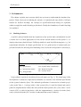
A model is always helpful when the complexity of the system under consideration exceeds
a certain level. It is then appropriate to focus on the relevant features of the system, i.e., to
abstract unnecessary details from it. Different models are used for different purposes, e.g., for
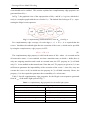
requirements definition, for design specification, etc. It is good practice to analyze and compare these models for detecting and eliminating errors, before the final product is released [9].
Legend:
Spec: Specification
SUC: System under consideration
MSpec: Specification model
MBhv: Behavioral model
MDsgn: Design model
MSyst: System model
Fig. 1. Simplified process of software development
Large software systems are developed in several stages (see Fig. 1). The initial stage of the
development is usually the requirements definition; its outcome is the informal specification
of the system’s behavior (Spec). The informal specification is converted to a formal specification model (MSpec). A design model of the system (MDsgn) is then developed and used to
guide the implementation efforts that will yield the actual product, the system under consideration (SUC) as called in this thesis. After the implementation, a behavioral model (MBhv)
can be extracted from the SUC in order to understand the system’s behavior.
Preliminaries
-6-
In this thesis, the SUC will be modeled in two ways: the design model, and the behavioral
model. The term system model (MSyst) is used in this thesis as a synonym referring to MDsgn or
MBhv depending on the availability of the models.
3.1.1 Specification Model
During the requirements definition, a specification model (MSpec) prescribes the desirable
behavior as it should be, i.e., the functionality of the system in compliance with the requirements of the user. Using a simple, but a formal notation for MSpec is important to enable a discussion of the requirements with the user, and the deployment of MSpec for analysis and requirement validation purposes, respectively.
In this thesis event-based systems are considered instead of state-based systems, where the
user is rather interested in the external behavior (black-box behavior) of the SUC than in its
internal mechanism. Therefore, to specify the behavior of an event-based system, the developer and the user think in terms of system “events” instead of system “states”. So the notion
of event plays a central role.
An event is considered to be an externally observable phenomenon, such as an environmental or a user stimulus, or a system response, punctuating different stages of the system
activity. In this sense, let V be the set of all possible events in the specification. MSpec is then
represented as a digraph [7], which is introduced below.
Definition 1: An Event Sequence Graph (ESG) is a directed graph (V, E), with a finite set
of nodes V ≠ ∅ and a finite set of edges E ⊆ V × V.
MSpec interprets the ESG as follows: Any node v ∈ V is interpreted as an event or as a
stimulus (action) that triggers that event (in the rest of the thesis, the terms “event” and “action” will be used as synonyms) and each specified event is expected to be triggered at least
once. An edge e ∈ E connecting two consecutive events is interpreted as an event sequence.
For two events v and v’ in V, the event v’ must be executable (enabled) after the execution of
v, if v and v’ compose an event sequence, i.e. (v, v’) ∈ E. In this context, (v, v’) is interpreted
as a legal event sequence of the event sequencing relation E. Additionally, MSpec identifies a
node v0 ∈ V as the starting node.
A specification model MSpec = (VSpec, ESpec, v0) defined as an ESG with a starting node v0 describes a set of sample behaviors of a system. Because the requirements of the user are specified in the early stages of behavioral modeling, the outcoming specification model may not be
Preliminaries
-7-
complete. As the design phase evolves, the present specification model can be modified or
extended depending on the changing requirements of the user.
It is also possible to define forbidden scenarios with ESG, i.e., ones that are not allowed to
happen. This complementary view of the requirements specification (holistic view, will be
introduced in section 3.2.3) helps to differentiate between desired and undesired system
behavior. Based on Definition 1 and its interpretation above, the complementary specification
model of MSpec is formally represented by another ESG M’Spec = (VSpec, E’Spec, v0) where
− VSpec represents the same set of events of MSpec,
− E’Spec = VSpec × VSpec \ ESpec contains all complementary event sequences not included in
ESpec where any (v, v’) ∈ E’Spec is interpreted as an illegal event sequence,
− v0 ∈ VSpec is the same initial node of MSpec.
3.1.2 System Behavior Model
For verification purposes the behavior of the SUC has to be modeled. Modeling the system
behavior can be considered in two ways: Firstly, a modeler can produce an abstraction of the
desired system functions in the design phase of a development process, which the developer
will then use as guidance to produce the end product, the SUC. This kind of model will be
called a design model (MDsgn).
Secondly, the behavior of an existing system can be analyzed and described as a behavioral
model (MBhv). MBhv is constructed from the view of the user in several steps, incrementally increasing his/her intuitive cognition of the SUC, usually by experimenting without any primary
knowledge about its structure. In this thesis, an intuitive way of the construction of MBhv has
been considered. Proposals also exist, however, for automating the model construction, e.g.,
in [30], applying learning theory. Taking these proposals into account would further rationalize the approach; however, it is not in the scope of this thesis. In both cases MSyst will be
modeled as a finite state machine [23].
Definition 2: A finite state machine (FSM) is a quadruple (S, S0, A, R), where
−
S is a set of states,
−
S0 is a set of start states, where S0 ⊆ S,
−
A is an input alphabet,
−
R is a transition relation that maps an input symbol a ∈ A and a current state s ∈ S to a next
state s´ ∈ S, i.e. R(s, a) ∈ S.
Preliminaries
-8-
Since the approach introduced in this thesis uses model checking as the verification
method, MSyst will have to be converted into a Kripke structure (see section 3.3.1). Conversion
from the actual formalism into Kripke structure will be explained in section 4.1.
3.2
Specification-Based Testing
Specification-based testing refers to the process of testing a program, based on what its
specification says its behavior should be. In particular, test cases can be developed based on
the specification of the program's behavior, without having an implementation of the program
(black-box testing). Furthermore, test cases can be developed before the program even exists.
There is also another type of testing – implementation-oriented testing – where the source
code of the software is taken into account by generating test cases (white-box testing).
There are two main roles a specification can play in software testing [32]. The first is to
provide the necessary information to check whether the observed behavior of the program is
correct. Checking the correctness of program behavior is known as the oracle problem. The
second is to provide information to select test cases and to measure test adequacy. This section focuses on both aspects of using a specification for generating test cases.
3.2.1 Test Case Generation
It makes sense to construct test cases, in compliance with the tester’s expectations of how
the system should behave, during the early stages of the integrated software development
process, long before the implementation begins. The generated test cases can then be run at
the end of the development process without any knowledge of the implementation. During
each phase of software development, formal specifications of the software, e.g. finite-state
machines, can be used to generate test cases. There are numerous approaches to generate test
cases from finite-state machines [3, 12, 17].
However, if testing is done from a user’s point of view, internal specifications can not be
used for test case generation, since the user has no insight into the development process. The
only reference for the software functionality is the user manual, which is mostly formulated
in an informal descriptive language. The user manual can also be seen as an informal
specification or as a system description. The challenge in testing is to include user’s
expectations and behavior into the testing, using this informal system description. As the user
should obey the descriptions in the user manual, it can be used as a source for test case
Preliminaries
-9-
generation. Thus the system is tested against the user manual. If there are discrepancy
between the system description in the user manual and the system behavior, an error is found.
As introduced in chapter 2, a test case is a tuple of a test input and an expected test output.
In this thesis the test inputs are the event sequences specified by MSpec and its complement
M’Spec as defined in 3.1.1. The expected test output is defined by the legality of the event sequence. The legal event sequences from MSpec represented with the edges of the ESG should
be executable on the system; on the other hand the illegal event sequences from M’Spec represented by the complementary edges of the ESG should not be executable on the system.
In specification-based testing a set of test cases (test suite) is produced on the basis of a
specification. The existence of a formal specification makes the automatic generation of test
suites possible. Usually a test suite should satisfy a given property, a criterion specifying
when to stop testing. Such a criterion could simply refer to some notion of coverage. The next
section explains more about test coverage and its uses.
3.2.2 Test Coverage and Spanning Set
Regardless of whether testing is specification-oriented or implementation-oriented, if applied to large programs in practice, both methods need an adequacy criterion, which provides
a measure of how effective a test suite is, in terms of its potential to reveal faults [32]. During
the last decades, many adequacy criteria have been introduced. Most of them are coverageoriented, i.e., they rate the portion of the system specification or implementation that is covered by the given test suite in relation to the uncovered portion when this test suite is applied
to the SUC. This ratio can then be used as a decisive factor in determining the point in time at
which to stop testing, i.e., to release the SUC or, to improve it and/or extend the test suite to
continue testing, which is called the test termination problem [4].
The approach in [4], which will be applied to model checking in this thesis, favors an adequacy criterion, based on specification-coverage, in order to handle the test termination problem. The test process can stop if all possible scenarios given by the specification are tested on
the SUC.
3.2.3 Holistic View
A short motivation for also considering the forbidden scenarios for testing and modeling
them is already made in section 3.1.1. This complementary view of the requirements specifi-
Preliminaries
- 10 -
cation is called the holistic view and is introduced in [4]. It helps to differentiate between desired and undesired system behavior.
The holistic approach to specification-based construction of test suites proposes the generation of all possible test cases that cover both the specified and not-specified properties of
the system, regardless of whether they are desirable or undesirable. As explained in section
3.1.1, the desirable behavior of the system is specified by MSpec and the undesirable behavior
of the system is specified by M’Spec.
The holistic view helps to clearly differentiate the correct system reaction from the faulty
one, as the test cases based on MSpec are to succeed the test, and the ones based on M’Spec are
to fail, when applied on the SUC. Thus, the approach handles the oracle problem, introduced
at the beginning this section, in an effective manner. Even if additional effort is needed for the
holistic view, by testing the unspecified system interaction the test engineer creates more
confidence in the SUC.
3.3
Model Checking
Model checking consists of three main steps [20]:
1. Modeling: The system model to be verified must be converted to a formalism accepted by
a model checking tool. The model can abstract the details that do not affect the correctness
of the checked properties.
2. Specification: The properties that the system model must satisfy should be stated. An
important point to consider is the completeness. That means, verifying a single property
does not cover all the properties that the system should satisfy.
3. Verification: This step is executed automatically by the model checker. The outcomes of
the two preceding steps are given to the model checker as input. The result of the verification step shows either that the model satisfies the property, or that the model does not satisfy the property, in which case further investigations are required.
3.3.1 Kripke Structure
Model checking uses a type of state transition graph called a Kripke structure to model a
system. A Kripke structure is basically a graph consisting of nodes representing the reachable
states of the system and edges representing the state transitions of the system. It also contains
a labeling of the states of the system with properties called atomic propositions that hold in
each state. A Kripke structure is formally defined as follows [20]:
Preliminaries
- 11 -
Definition 3: Let AP be a set of atomic propositions; a Kripke structure K over AP is a
quadruple K=(S, S0, R, L) where S is a finite set of states, S0 ⊆ S is the set of initial states, R ⊆
S×S is a transition relation such that for every state s ∈ S there is a state s’ ∈ S in that R(s, s’)
and L:S→2AP is a function that labels each state with the set of atomic propositions that are
true in that state [20].
A state of a Kripke structure is a snapshot or instantaneous description of the system that
capture the values of the variables at a particular point in time. There is also the need to know
how the state of a system changes as a result of some action of the system or user. The
changes in the state can be defined by giving the state before the action occurs and the state
after the action occurs. Such a pair of states determines a transition of the system. The computations of the system can be defined in term of its transitions. So the Kripke structure defines a state transition system [25].
3.3.2 Temporal Logic
Temporal logic is a formalism for describing sequences of transitions between states in a
reactive system and is traditionally interpreted in terms of Kripke structures. Reactive systems
need to interact with their environment frequently and often do not terminate. The behavior of
a reactive system emerges when the system responses to events generated by its environment
[20].
In the temporal logic considered here, time is not mentioned explicitly; instead, a formula
might specify that eventually some property holds or that some property never holds. Properties like eventually or never are specified using temporal operators. These operators can also
be combined with boolean connectives or nested arbitrarily. Temporal logics differ in the operators that they provide and the semantics of those operators [20].
Temporal logic can describe the order of events in time, which is expressed by means of
state transitions. Each transition represents a time unit. This is also called discrete time scale.
Temporal logics are often classified according to whether time is assumed to have a linear or
a branching structure. Temporal logic formulas can be interpreted over a state transition system, e.g. Kripke structure [20].
Computation tree logic (CTL*) formulas describe the properties of computation trees of
state transition systems. The tree is formed by choosing a state of the transition system as the
initial state and then unwinding the structure into an infinite tree, with the designated state at
the root. The computation tree shows all the possible executions of a system starting from the
Preliminaries
- 12 -
initial state. A path π is an infinite sequence of states (π = s0s1s2…) in the computation tree
[20].
In CTL*, the formulas are composed of path quantifiers and temporal operators. The path
quantifiers are used to describe the branching structure in the computation tree. There are two
such quantifiers A (“for all computation paths”) and E (“for some computation paths”). These
quantifiers are used in a particular state, to specify that all of the paths or some of the paths
starting at that state have a specific property. The temporal operators describe properties of a
path through the tree. There are five basic operators [20]:
–
X (neXt) requires that a property holds in the next state of the path.
–
F (Future) is used to assert that a property will hold at some state on the path.
–
G (Global) specifies that a property holds at every state on the path.
–
U (Until) holds if there is a state on the path where the second property holds, and the first
property holds at every preceding state on the path.
–
R (Release) is the logical dual of U. It requires that the second property holds along the path
up to and including the first state where the first property holds. However, the first property
is not required to hold eventually.
Path formulas define properties for computation paths of the Kripke structure. In order to
define some property for a state using path formula, path quantifiers are deployed. If f is a
path formula, Ef is a state formula. This formula is valid for a state s, if there is a path π beginning from s, where f is valid. Similarly Af is also a state formula, saying that on all paths
beginning from s, f must be true [20].
The two useful sublogics of CTL* are branching-time logic and linear-time logic. The distinction between the two lies in how they handle branching in the underlying computation
tree. In branching-time temporal logic, the temporal operators quantify over the paths that are
possible from a given state. In linear-time temporal logic, operators are provided to describe
events along a single computation path [20].
Definition 4: Computation Tree Logic (CTL) is a restricted subset of CTL* in which each
of the temporal operators X, F, G, U, and R must be immediately preceded by a path quantifier. In other words, CTL is the subset of CTL* that is obtained by restricting the syntax of
path formulas using the following rule:
− If f and g are state formulas, then X f, F f, G f, f U g, f R g are path formulas.
Definition 5: Linear Temporal Logic (LTL), on the other hand, consists of formulas that
have the form A f where f is a path formula in which the only state subformulas permitted, are
atomic propositions. An LTL formula is either:
Preliminaries
- 13 -
− p, where p is an atomic proposition, or
− a composition ¬f, f ∨ g, f ∧ g, X f, F f, G f, f U g, f R g [20].
In this thesis, both CTL and LTL formulas are used to specify system properties.
The system properties defined with temporal logic formulas can be grouped into classes
corresponding to their art of formulating the property. Three of these property classes are the
followings: Reachability properties, safety properties and liveness properties. Reachability
properties define system properties, saying that some state of the system with a desired property is reachable. Reachability properties can be formulated using “E” path quantifier in CTL.
A reachability property holds, if there is some execution of a system including a state where
the property holds. Liveness properties assure that a system executes as expected or that
“something good will eventually happen”. Safety properties on the other hand ensure that the
system does not enter an undesired state or that “something bad will not happen” [11].
3.3.3 Model Checker
A model checker explores the reachable state space of the model, specified as a Kripke
structure, and verifies whether the expected system properties, specified as temporal logic
formulae, are satisfied over each possible path. If a property is not satisfied, the model
checker answers with “invalid” and generates a counterexample in the form of a sequence of
states, called a trace [1, 20].
Counterexamples can be used to localize the error, by tracking down the trace until the state
where the error occurs. Analyzing the error trace may require an adaptation of the model and
a re-verification. Another reason for error can also be an incorrect modeling of the system or
an incorrect specification (false negative [20]). In each case further modifications on the
model or on the specification are required. After modifications, the model checking process
must be repeated.
Coverage-Driven Model Checking
- 14 -
4. Coverage-Driven Model Checking
The approach presented in this thesis aims to check the SUC against the user requirements,
just as validation and verification aim to do. This check can be done in different stages during
the software development process. Testing, for example, is mainly applied manually, after the
implementation of the SUC in its real environment; if errors are detected the SUC must be
debugged and the relevant portions of the program code must be corrected. Model checking
can be applied automatically on a system abstraction, to check whether the system abstraction
contains errors; in the case of software, this could be a design model; if there are some errors,
they are corrected on the design long before implementation. But what about gaining testing
information on the SUC before implementation or applying model checking after the SUC is
implemented? Combining both methods as explained in this thesis has the advantage that
testing activities can be transferred into early stages of the development process and can be
automated.
To put it more precisely, the approach realizes a coverage-based test adequacy criterion [5,
6, 32] as explained in section 3.2 on MSyst by using model checking. A set of properties are derived from MSpec and model checked on MSyst. Since the properties are produced from
specification-based test cases, the model checking step effectively performs a testing activity
on MSyst. Additionally, the approach systematizes the model checking process and handles the
completeness problem of the checked properties, with respect to the specification-based test
adequacy criterion known for long in testing community. It is important to notice that this
approach involves no testing activity in a classical manner because the SUC is not tested
directly. The concepts of testing are applied to model checking.
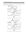
Fig. 2 and Fig. 3 show different aspects and the structure of the approach, which are illustrated as UML-Activity diagrams [27], including control-flow (solid lines) for activities and
data-flow (dashed lines) for the inputs/outputs of the activities.
The approach described in Fig. 2 assumes that the user of the approach has access to the
MDsgn during the development process as an output of the design phase, which will be called
MSyst. Firstly, the requirements on the SUC are defined; the outcome is the informal specification Spec. After analyzing the requirements, the development process forks into two phases:
During the SUC is designed, from the formalized specification MSpec and its complement
M’Spec, system properties are generated that will be checked on MSyst. If model checking shows
unconformities, then either the design process should be repeated or the requirements should
Coverage-Driven Model Checking
- 15 -
be checked. Thus the start of the testing activities is pushed back in the software development
process by using model checking. In other words, the purpose of testing is carried out on the
system model by using model checking.
Fig. 2. Overall structure of the approach using the design model
Fig. 3. Overall structure of the approach using the behavioral model
Coverage-Driven Model Checking
- 16 -
Fig. 3 assumes that the user of the approach has no access to the development process; so
the SUC is a black-box for the user. The only functional description is the user manual of the
SUC. In this case two independent activities take place; firstly, by means of the black-box
SUC an abstract behavioral model (MBhv) is generated, which will be called MSyst. Secondly,
from the informal specification a formal specification model is generated from which the
system properties are extracted. The later step is similar to the one in Fig. 2.
The general approach introduced above will be applied in this thesis on a specific case
where for an event-based application system properties are generated from event sequences
specified by MSpec and M’Spec. Each event sequence is interpreted as a test input of a test case.
Whether the event sequence is legal or illegal, the test output is defined as executable or notexecutable. From the test inputs, system properties are produced in the form of temporal logic
formulae. Based on the holistic approach, both the specified event sequences and the unspecified event sequences are considered by generating the system properties. The number of generated system properties is limited by the size of the specification, so the model checking
process can be ended when all system properties are checked; thus the completeness problem
is handled.
In the rest of this chapter the approach illustrated in Fig. 2 and Fig. 3 is explained in detail
using a simple example. Section 4.1 shows how a system model can be converted into a
Kripke structure for model checking purposes. Section 4.2 introduces a simple example “traffic light system” which will be used in the rest of the chapter. Section 4.3 explains the concept
of coverage-based adequacy criterion and its adaptation to model checking, by introducing the
terms node coverage, edge coverage and the complementary view of the edge coverage. Section 4.4 introduces a new term check case and explains its generation and its meaning for the
approach. Section 4.5 describes the model checking process of the check cases. Section 4.6
gives an overview of the complexity of the approach.
4.1
Converting the System Model into a Kripke Structure
In order to verify the system properties generated from MSpec = (VSpec, ESpec, v0) on MSyst =
(SSyst, SSyst0, ASyst, RSyst), MSyst has to be converted to a Kripke structure given by a quadruple K
= (S, S0, R, L) defined over a set of atomic propositions AP. AP includes two atomic propositions ven and vex for each event v ∈ VSpecc, semantically corresponding to “v is enabled” and “v
is executed” respectively. The set of states S of the Kripke structure will be labeled with these
atomic propositions signifying that whether the event v is enabled or executed at that state. In
Coverage-Driven Model Checking
- 17 -
order to differentiate between states where events are enabled or executed, S is divided into
two sets of states: SNS and STS, standing for normal states and transition states, respectively.
For any state s ∈ SSyst, there is a corresponding normal state s ∈ SNS. Furthermore, for any two
states s and s’ ∈ SSyst if it is possible to execute an event v ∈ ASyst at s, and execution of v at s
results in a state transition to s’, i.e. if RSyst (s, v) = s’∈ SSyst, then
i) there is a transition state svs’ ∈ STS ,
ii) (s, svs’) ∈ R,
iii) (svs’, s’) ∈ R,
iv) ven ∈ L(s) and
v) vex ∈ L(svs’).
S, R, and L include no elements other than the ones given above. Finally, S0 includes the
normal states corresponding to the initial states SSyst0. This thesis assumes a correct conversion
from MSyst into a Kripke structure, where the conversion itself could be a source of error for
the verification step.
4.2
Example “Traffic Light System”
This section introduces a small example “traffic light system”, taken from [29], which will
be used to illustrate the approach in the rest of this chapter.
The desired functionality of a traffic light system is as follows: Beginning with the color
red stopping the traffic flow, it changes to red/yellow and then to green allowing the traffic to
flow. After green it changes to yellow and then again to red. It is assumed that an external
actor, e.g. a controller, triggers some events in order to change the state of the traffic light.
The desired system function will be translated into a formal specification. A faulty system
model is also constructed in order to show how the approach operates.
The informal specification above can be formalized with a specification model MSpec =
(VSpec, ESpec, v0) where
− VSpec: {red, red/yellow, green, yellow},
− ESpec: {(red, red/yellow), (red/yellow, green), (green, yellow), (yellow, red)},
− v0: red.
Fig. 4 depicts MSpec graphically in the form of an ESG.
Coverage-Driven Model Checking
- 18 -
Fig. 4. Traffic light system specification as an ESG
A supposedly faulty MSyst for the traffic light system is given in Fig. 5 in the form of a
FSM. The states of MSyst represent the colors of the traffic light system. The transitions represent the color changes of the traffic light system. The fault in MSyst is obvious: The state where
the traffic light changes to “red/yellow” is missing. Such a fault is useful to demonstrate how
the approach localizes the injected fault.
Fig. 5. A faulty MSyst as a FSM
Fig. 6 transfers the FSM in Fig. 5 into a Kripke structure. The Kripke structure conserves
the three states red, green and yellow of MSyst as normal states SNS, but rename them as s1, s2
and s3. Additionally three transition states (s4, s5, s6) are generated for each transition in MSyst.
The atomic propositions generated from the events specified in MSpec are assigned to normal
and transition states, expressing either being enabled or executed at that state. For example,
considering the state transition (red, yellow) in Fig. 5, the event yellow must be enabled at
state s1 of the Kripke structure corresponding to the state red in MSyst; thus s1 is labeled with
the atomic proposition yellowen. The additional transition state s4 represents the point of time
where the event yellow is executed; thus it is labeled with the atomic proposition yellowex.
Fig. 6. Kripke structure for MSyst of Fig. 5
- 19 -
Coverage-Driven Model Checking
Formally, the Kripke structure is defined as a quadruple K = (S, S0, R, L) where
− S = {s1, s2, s3, s4, s5, s6} (where SNS = {s1, s2, s3} and STS = {s4, s5, s6}),
− S0 = {s1},
− R = {(s1, s4),(s4, s3),(s3, s5),(s5, s1),(s2, s6),(s6, s3)},
− L(s1)={yellowen},
L(s2)={yellowen},
L(s3)={reden},
L(s4)={yellowex},
L(s5)={redex},
L(s6)={yellowex}.
4.3
Covering the Specification Model
As explained in section 3.2.2, adequacy criterion is an important issue in software testing,
because the tester has to know when to stop testing the SUC. As mentioned earlier, a system
can not be tested completely; so an adequacy criterion is needed to determine the end of the
test process. Similarly in model checking, the completeness of the verified properties must be
considered in order to stop the verification step. Completeness in this context is defined as a
complete set of system properties specified by a formal specification model.
As mentioned in earlier sections, the approach considers an event-based system, where the
system-environment interactions are specified with an ESG. The nodes of the ESG represent
the events or the actions that trigger the events. For testing purposes, each action specified
with a node in ESG should be checked for executability. If it will never be executed, an
unconformity is detected. Two nodes of the ESG connected with an edge represent an event
sequence. For testing purposes, a legal event sequence requires that the action referring to the
second event should be executable just after executing the action referring to the first event. If
this is not the case, an unconformity is detected. Complementing the ESG produces new
edges, which are not included in the original ESG. The edges of the complemented graph
represent the illegal event sequences of the system interaction. For testing purposes, an illegal
event sequence requires that the action referring to the second event should not be executable
after the action corresponding to the first event is executed.
The selection of the test cases is carried out by applying the node coverage and edge coverage criteria to MSpec = (VSpec, ESpec, v0) and M’Spec = (VSpec, E’Spec, v0): The criteria requires all
nodes and edges to be covered by test cases, where, according to the semantics of ESG (compare with section 3.1.1), covering a node v ∈ VSpec means to test the executability of the event
v; covering an edge (v, v’) ∈ ESpec means to test the executability of v’ right after v is executed. Moreover, the approach complementarily requires the testing of the impossibility of an
event sequence (v, v’) when (v, v’) ∈ E’Spec. The distinction between initial node v0 and the
- 20 -
Coverage-Driven Model Checking
other nodes is not relevant for the property generation and will not be considered any further.
The generation of the system properties by using MSpec and M’Spec will be explained in the
following sections. The traffic light system from section 4.2 will be used as an example for
generating system properties.
4.3.1 Node Coverage
For achieving the adequacy criterion all nodes from VSpec of MSpec must be covered by the
generation of system properties. Node coverage can be seen as a reachability property
requiring that a state is reachable where an action triggering the specified event is executed.
Reachability properties are defined in CTL with EF operator. This section explains how node
properties are generated from MSpec.
For the node coverage, for each event v ∈ VSpec, it is required to check if the event v is ever
executable in MSyst which can be specified by the CTL formula:
EF vex
(1)
This node property is valid if v is executed in some reachable state of MSyst. Since, by definition, vex holds only at transition states of MSyst, the property “EFvex” successes if there exists
a path along which v is ever executed.
Table 1 lists all node properties generated from MSpec of the traffic light system in Fig. 4.
Table 1. Node properties for the traffic light system
Node Properties
EF redex
EF redyellowex
EF greenex
EF yellowex
4.3.2 Edge Coverage
For achieving the adequacy criterion all edges from ESpec of MSpec must be covered by the
generation of system properties. Edge coverage can be seen as a liveness property, requiring
that a legal event sequence is possible in the system, i.e. the second event of an event sequence is enabled after the first event is executed. Liveness properties can be defined in LTL
with the temporal operator G, specifying the property on every state of a computation path.
This section explains how edge properties are generated from MSpec.
- 21 -
Coverage-Driven Model Checking
For achieving the edge coverage, for each edge (v, v’) ∈ ESpec, it is necessary to check if the
event v’ is enabled right after the executions of the event v, which can be specified by using
the LTL formula:
G (vex → X v’en)
(2)
This edge property is valid on the states in MSyst where v is executed and at all consecutive
states v’ is enabled. As from a transition state, at which vex holds, there is only one outgoing
transition and it ends at a normal state, the edge property in (2) will hold only if v’ is enabled
at that normal state. Note that, an edge property as given in (2) is not sufficient to guarantee
the executability of the event v’, since MSyst may not execute the event v at all, in which case
the property in (2) will hold vacuously. Hence, the property (1) is also required to guarantee
the executability of v at least once.
Table 2 lists all edge properties for the legal event sequences generated from MSpec of the
traffic light system in Fig. 4.
Table 2. Edge properties for the traffic light system
Edge Properties
G (redex → X redyellowen)
G (redyellowex → X greenen)
G (greenex → X yellowen)
G (yellowex → X reden)
4.3.3 Complementing the Edge Coverage
The approach can be extended by the holistic view of edge coverage where the complementary specification model M’Spec = (VSpec, E’Spec, v0) is also considered by property
generation. M’Spec completes the missing edges in MSpec from Fig. 4 by adding new edges to
the ESG wherever possible, as illustrated in by dashed lines in Fig. 7. Additional system
properties can be generated based on these complementary edges from E’Spec. These
additional system properties are used to get a full coverage of the properties based on both the
requirements, incorporated by original edges and anti-requirements, incorporated by
complementary edges, thus leading to a completeness of model checking with respect to the
given specification model. The complementary edge properties can be seen as safety
properties, which specify that after the first event of an event sequence is executed the second
- 22 -
Coverage-Driven Model Checking
event should not be enabled. This section explains how complementary edge properties are
generated from M’Spec.
In Fig. 7, the graphical view of the superposition of MSpec and M’Spec is given, which obviously is a complete graph with the set of nodes VSpec. The dashed lines belong to E’Spec, representing the illegal event sequences.
Fig. 7. Complementing (with dashed lines) of the MSpec from Fig. 4
For complementary edge coverage, for each edge (v, v’) ∈ E’Spec, it is required that the
event v’ should not be enabled right after the execution of the event v, which can be specified
by using the complementary edge property in LTL:
G (vex → X ¬v’en)
(3)
The complementary edge property is valid on the states of MSyst where v is executed and at
all consecutive states v’ is not enabled. As from a transition state, at which vex holds, there is
only one outgoing transition and it ends at a normal state, the LTL property in (3) will hold
only if v’ is not enabled at that normal state. Note that, an LTL property as given in (3) is not
sufficient to guarantee the impossibility of the execution of the event v’, since MSyst may not
execute the event v at all, in which case the property in (3) will hold vacuously. Hence, the
property (1) is also required to guarantee the executability of v at least once.
Table 3 lists all complementary edge properties for the illegal event sequences generated
from M’Spec of the traffic light system in Fig. 7.
Table 3. Complementary edge properties for the traffic light system
Complementary Edge Properties
G (redex → X ¬greenen)
G (greenex → X ¬reden)
G (redex → X ¬yellowen)
G (greenex → X ¬redyellowen)
G (redex → X ¬reden)
G (greenex → X ¬greenen)
G (redyellowex → X ¬reden)
G (yellowex → X ¬redyellowen)
G (redyellowex → X ¬yellowen)
G (yellowex → X ¬greenen)
G (redyellowex → X ¬redyellowen)
G (yellowex → X ¬yellowen)
- 23 -
Coverage-Driven Model Checking
4.4
“Check Cases” and their Generation
The term check case emphasizes here the combination of the terms “model checking” and
“test case”. In analogy to a test case as introduced in chapter 2, the system property f is the
input of the model checking (in addition to the model to be checked), whereby the expected
output is specified as a binary value defined as follows:
Definition 6: A temporal logic formula f, as a property of a Kripke structure K, is valid, if
K satisfies the property f. Otherwise, f is invalid. Check results CR = {valid, invalid} is a set
containing both the values a property f can get if model checked on K.
Definition 6 enables the presentation of test cases as a combination of a temporal logic formula and a binary value as given in the following definition:
Definition 7: A check case is an ordered pair (f, cr) where f is a system property based on a
node property or an edge property of MSpec or a complementary edge property of M’Spec and cr
∈ CR is a check result.
From the system properties generated for the traffic light system in sections 4.3.1 - 4.3.3 the
check cases in Table 4 can be generated.
Table 4. Check cases generated from the system properties of the traffic light system
Node Properties
Edge Properties
cr1 = (EF redex, valid)
cr5 = (G (redex → X redyellowen) , valid)
cr2 = (EF redyellowex, valid)
cr6 = (G (redyellowex → X greenen) , valid)
cr3 = (EF greenex, valid)
cr7 = (G (greenex → X yellowen) , valid)
cr4 = (EF yellowex, valid)
cr8 = (G (yellowex → X reden) , valid)
Complementary Edge Properties
cr9 = (G (redex → X ¬greenen) , valid)
cr15 = (G (greenex → X ¬reden) , valid)
cr10 = (G (redex → X ¬yellowen) , valid)
cr16 = (G (greenex → X ¬redyellowen) , valid)
cr11 = (G (redex → X ¬reden) , valid)
cr17 = (G (greenex → X ¬greenen) , valid)
cr12 = (G (redyellowex → X ¬reden) , valid)
cr18 = (G (yellowex → X ¬redyellowen) ,
valid)
cr13 = (G (redyellowex → X ¬yellowen) , valid)
cr19 = (G (yellowex → X ¬greenen) , valid)
cr14 = (G (redyellowex → X ¬redyellowen) , valid)
cr20 = (G (yellowex → X ¬yellowen) , valid)
- 24 -
Coverage-Driven Model Checking
4.5
Model Checking of “Check Cases”
The system property of a check case is model checked and the result is compared with the
expected check result of the check case. Whenever model checking reveals an inconsistency,
an error is detected. This can, in turn, be caused by an error in MSyst, MSpec, or Spec. These
inconsistencies, if any, are the key factors of fault localization, which is a straight-forward
process: Check whether the inconsistency is caused by an error in MSyst. If the cause of the
inconsistency is located in MSyst, an error in the developer’s understanding of the system requirements is revealed, which must be corrected, i.e., MSyst is to be “repaired”. Other sources
of errors are the specification and MSpec, which are to be checked in the same way.
The manual model checking of MSyst of the traffic light system is sketched in Table 5
including all properties based on MSpec and M’Spec. The results of the analysis of Table 5 are
summarized as follows: 4 of 20 check cases lead to inconsistencies in MSyst. Thus, model
checking detected all of the injected faults.
Table 5. Manual model checking of system properties
System Properties
cr1 = (EF redex, valid)
+
cr2 = (EF redyellowex, valid)
-
cr3 = (EF greenex, valid)
-
cr4 = (EF yellowex, valid)
+
cr5 = (G (redex → X redyellowen) , valid)
-
cr6 = (G (redyellowex → X greenen) , valid)
+
cr7 = (G (greenex → X yellowen) , valid)
+
cr8 = (G (yellowex → X reden) , valid)
+
cr9 = (G (redex → X ¬greenen) , valid)
+
cr10 = (G (redex → X ¬yellowen) , valid)
-
cr11 = (G (redex → X ¬reden) , valid)
+
cr12 = (G (redyellowex → X ¬reden) , valid)
+
cr13 = (G (redyellowex → X ¬yellowen) , valid)
+
cr14 = (G (redyellowex → X ¬redyellowen) , valid)
+
cr15 = (G (greenex → X ¬reden) , valid)
+
cr16 = (G (greenex → X ¬redyellowen) , valid)
+
cr17 = (G (greenex → X ¬greenen) , valid)
+
cr18 = (G (yellowex → X ¬redyellowen) , valid)
+
cr19 = (G (yellowex → X ¬greenen) , valid)
+
cr20 = (G (yellowex → X ¬yellowen) , valid)
+
Legend: +: the check case passes; -: the check case fails
Coverage-Driven Model Checking
4.6
- 25 -
Complexity Analysis of the Approach
Since there are a finite set of nodes and a finite set of edges in MSpec, the number of properties to be checked on MSyst is also finite. The number of system properties by node coverage
increases linearly with the number of events, whereas the number of system properties by
edge coverage increases exponentially with the number of events. The number of events can
be controlled by abstracting the system or by handling the system functions separately.
[31] implies that the complexity of the automata-based LTL model checking algorithm increases exponentially in time with the size of the formula (| f |), but linearly with the size of
the model (|S|+|R|). The complexity of LTL model checking is O(2| f |×(|S|+|R|)), where
− size of the formula (| f |): the number of symbols (propositions, logical connectives and
temporal operators) appearing in the representation of the formula,
− size of the model (|S|+|R|): the number of elements in the set of states S added with the number of elements in the set of transitions R.
Based on this result, the complexity of LTL model checking might be acceptable for short
LTL formulas. Additionally the size of the model should be also controllable to avoid the
state space explosion problem.
For the present approach, LTL model checking is deployed for each formula f generated
from legal and illegal event sequences of MSpec and M’Spec. The number of all legal and illegal
event sequences is |VSpec|×|VSpec| = |VSpec|2. As explained in sections 4.3.2 and 4.3.3, the properties have always the same pattern: Globally, if some property p holds at some state, at the next
state a property q should either hold in case of a legal event sequence (G(p →Xq)), or should
not hold in case of an illegal event sequence (G(p →X¬q)). The size of the formulas (| f |) is
always constant. Because of this fact, the exponential growth of the complexity of LTL model
checking can be ignored and the resulting complexity is O(|VSpec|2×(|SSyst|+|RSyst|)).
Additionally CTL model checking is deployed for each formula f generated from nodes of
MSpec. The number of all nodes is |VSpec|. [19] implies that the complexity of the CTL model
checking is O((|S|+|R|)×| f |. Since the node properties always have the form EFp, the size of
the formulas (| f |) is always constant; thus the complexity depends just on the size of MSyst:
O(|SSyst|+|RSyst|).
After adding the complexities of model checking both the node properties and the edge
properties, the overall complexity of the approach is measured as O(|VSpec|2×(|SSyst|+|RSyst|)).
Case Study and Tool Support
- 26 -
5. Case Study and Tool Support
In order to show the applicability of the approach to a non-trivial system, a case study is
carried out. Applications with a graphical user interface (GUI) are suitable to be checked by
the approach, because the user interacts with the system via events. The user can trigger these
events via graphical components called WIMPs (Windows, Icons, Menus, and Pointers), like
buttons.
Fig. 8. Top menu of the RealJukebox (RJB)
Fig. 8 represents the utmost top menu as a GUI of the RealJukebox (RJB -- RealJukebox 2
® Build: 1.0.2.340 Copyright © 1995-2000 RealNetworks ™. Inc.). RJB has been introduced
as a personal music management system. The user can build, manage, and play his or her individual digital music library on a personal computer. At the top level, the GUI has a pull-down
menu that includes many functions. For some of the mostly utilized functions there are
buttons as short-cuts on the top level GUI. The graphical representation of the buttons gives
an intuitive understanding of the availability of the corresponding function. After a button is
pressed, either the button returns to its initial enabled state which makes it pressable again, or
- 27 -
Case Study and Tool Support
the button remains pressed and is disabled until some other action is taken which enables the
button again.
As the code of the RJB is not available, only black-box methodologies are applicable to
validate the behavior of the RJB. In order to apply the introduced approach on RJB, firstly the
behavioral system model MSyst of RJB is produced by observing the system. MSyst can be produced by experimenting with the system and identifying the system states and the appearance
of the graphical components at these states that trigger the system events.
Secondly, a specification model MSpec is required for the approach. The user manual of RJB
is used to produce the MSpec. The production of MSpec for RJB in the form of ESG’s is explained in [10] where the same case study is used to demonstrate a testing technique. In [10],
RJB is tested manually with the test cases derived from ESG’s and some errors are found. The
approach introduced in this thesis is different than the approach in [10], in relation to the fact
that the actual system will not be tested directly; the approach verifies properties on an abstraction of the system. In section 5.4 the found errors in [10] are compared to the ones found
with the approach in this thesis.
5.1
Specification Model
Because there is no system specification of RJB available to the end user, the user manual
facilities of RJB are used to produce references for construction of specification models [10].
Specification models are produced and incrementally extended in terms of ESG’s, which are
very rudimentary at the beginning but they are refined later on. The constructed ESG’s are
grouped into 13 system functions that are listed in Table 6.
Table 6. System functions of RJB
1. Play and Record a CD or Track
8. Skins
2. Create and Play a Playlist
9. Screen Sizes
3. Edit Playlists and/or Auto-Playlists
10. Different Views of Windows
4. Views Lists and/or Tracks
11. Find Music
5. Edit a Track
12. Configure RJB
6. Visit the Sites
13. Configuration Wizard
7. Visualization
Case Study and Tool Support
- 28 -
Each system function, represented as an ESG, serves as a specification model MSpec for the
approach. As an example, the MSpec in Fig. 9 specifies the top-level GUI interaction for the desired system function “Play and Record a CD or Track”. The user can play/pause/record/stop
the track, fast forward and rewind. Fig. 9 illustrates all legal event sequences related to usersystem interaction, which realize the operations the user might launch when using this system
function. The main functionality is specified by the utmost-level ESG RJB1.
Play Track
Fig. 9. MSpec for the system function “Play and Record a CD or Track”
Because of the large amount of possible interaction sequences given in the user manual for
this system function, related system event sequences are grouped into other ESG’s, e.g. Select
Track, which are then used as pseudo-events in the main ESG RJB1. As a convention the
pseudo-events are identified by a capitol letter distinguishing them from system events. Apart
from the internal event sequences in ESG Select Track, an edge from the pseudo-event Select
Track to itself in ESG RJB1 makes all combinations of event sequences in ESG Select Track
possible. Similarly, an edge from Select Track to Mode in RJB1 makes all combinations of
Case Study and Tool Support
- 29 -
event sequences between the two ESG’s possible. The complementary specification model
M’Spec can be easily produced by adding the missing edges in ESG’s.
For computation purposes each ESG is represented as an adjacency matrix stored in a plain
text file (specification file). The specification files contain semicolon separated data; an edge
between two nodes, representing a legal event sequence, is indicated as “1”. If there is no
edge between the two nodes, a “0” is used indicating an illegal event sequence. Table 7 shows
the specification file of the top-level ESG RJB1.
Table 7. Specification file of the top-level ESG RJB1
RJB1;SelectTrack;Mode;PlayTrack;
1;1;1;
1;1;1;
1;1;1;
The first line of the specification file contains the name of the ESG RJB1 and the node labels SelectTrack, Mode and PlayTrack. The node labels identify also columns and rows
of the adjacency matrix. Because the row identifiers are the same as the column identifiers,
they are only given once in the first line of the specification file.
Similarly Table 8 shows the specification file of the sub-level ESG Play Track in RJB1. In
the first line, the name of the ESG and the system events are given. Track is again a pseudoevent representing the group of all events related to switching between tracks and changing
the track position. The specification files of all ESG’s can be found in Appendix A.
Table 8. Specification file of the sub-level ESG Play Track
PlayTrack;play;pause;record;stop;Track;
0;1;0;1;1;
1;0;0;1;1;
1;0;0;1;0;
1;0;1;0;1;
1;1;1;1;1;
Case Study and Tool Support
5.2
- 30 -
System Model
As we have no insight into the development process of the commercial software RJB, a behavioral model MBhv will be used as system model MSyst instead of MDsgn; thus the approach is
applicable in the form as illustrated and explained in Fig. 3 and in section 4 respectively. MSyst
will be produced by observing the functional behavior and the changes in the structure of
RJB.
The construction of MSyst for RJB can be explained as follows: Firstly, by playing with RJB
some system states are identified. These are the initial-state, the playing-state, the pausedstate, the recording-state and the stopped-state. Because the initial-state has the same appearance as the stopped-state which is reached if some function is canceled via stop-button, both
states are merged into the stopped-state.
Secondly, the state changes are analyzed by clicking the buttons of the GUI which leads to
a FSM like in Fig. 10. This system model observes only the system states and the system
events relating to the system function “Play and Record a CD or Track”. The transitions are
labeled with the corresponding names of the buttons that trigger the events and cause the state
changes.
Fig. 10. System model of RJB as a FSM
For verification purposes some additional information about the system model is needed.
Beside the dynamic properties of the system, some structural information about the system
states is collected by observing the appearance of the graphical components at each state. For
example a button object on the GUI can be disabled at certain states, which makes the functionality behind this button not-executable at these states.
Case Study and Tool Support
- 31 -
Using dynamic and structural properties, the system model is translated into a Kripke
structure in Fig. 11, as explained in section 4.1. The states of the FSM are conserved and converted to normal states in Kripke structure. The executability of the system events are represented as atomic propositions, e.g. at state stopped the play-button is enabled and can be
pressed, which is represented with the atomic proposition playen. If some state is not labeled
with playen, that means the play-button is either disabled or not visible at this state. Some
events are grouped into pseudo-events for efficiency purposes. For example the label
SelectTracken is a macro definition combining all atomic propositions for all events related to
the ESG Select Track in Fig. 9.
Fig. 11. MSyst of the top GUI level of the RJB
The transition information in FSM normally gets lost during translation of the system
model into a Kripke structure, because by definition 3, Kripke structures do not entail a
labeled transition relation. However, in order to keep this information, transition states are
added to the Kripke structure as explained in section 3.3.1. For each transition in the FSM, a
transition state in the Kripke structure is added and labeled with an atomic proposition
indicating the transition label. For example, if the transition from stopped-state to playingstate in the system model is triggered by the play-button, then the corresponding transition
state is labeled with the atomic proposition playex. The transition states have no logical names
like playing or stopped; they are named with a consecutive number. Fig. 11 depicts MSyst as a
Kripke structure of the same abstraction level as Fig. 10.
Case Study and Tool Support
- 32 -
For model checking the Kripke structure must be translated into a formalism that is accepted by the selected model checking tool. In this case study the model checker NuSMV is
selected for many reasons, which are addressed in the next section. NuSMV accepts the
Kripke structure in the form of a labeled transition system, which is also explained in the next
section.
5.3
Tool Support
Using the specification model and the system model, the generation and verification of the
system properties using tool support can begin. For tool deployment both models must be
converted into a machine-readable format. As explained in section 5.1 the specification model
is saved in plain text files, which include the adjacency matrix representations of the ESG’s.
The system model will be translated into a labeled transition system and also saved in plain
text. A small Java application given in Appendix B generates system properties from the
specification model. Both the transition system and the system properties are merged in an
additional text file, which will be the input for the model checker NuSMV.
NuSMV [18] is a symbolic model checker, which originates from the reengineering, reimplementation and extension of SMV, the original BDD-based model checker developed at
CMU [26]. NuSMV is able to process files written in an extension of the SMV language. In
this language, it is possible to describe labeled transition systems by means of declaration and
instantiation mechanisms for modules and processes, corresponding to synchronous and asynchronous composition, and to express a set of system properties in CTL and LTL. NuSMV
can work batch or interactively, with a textual interaction shell.
A NuSMV program is composed of modules. A module is an encapsulated collection of
declarations. Once defined, a module can be reused as many times as necessary. Furthermore,
each instance of a module can refer to different data values. A module can contain instances
of other modules, allowing a structural hierarchy to be built. A process is a module which is
instantiated using the keyword process. The program executes a step by non-deterministically choosing a process and then executing all of the assignment statements in that process
specified with keyword ASSIGN. There are two kind of assignment statements: init() and
next(). init() denotes the initial state of some variable. next() assigns to the variable its
value at the next state. It is implicit that if a given variable is not assigned a new value by the
process, then its value remains unchanged.
Case Study and Tool Support
- 33 -
5.3.1 Representation of System Model
In this section the representation of the Kripke structure as a labeled transition system in
NuSMV language is explained. Small portions of codes are given as examples for understanding the syntax.
In each NuSMV code, there must be one module with the name main. The module main
is evaluated by the interpreter. Therefore, the Kripke structure representing the system model
of RJB from Fig. 11 is translated as a single process into a main module (see Fig. 12), which
includes assignment statements specifying the initial values of the state variables and the transition relation between the system states. The NuSMV code in Fig. 12 is not complete; the
missing code portions are represented with “…”. This section of the thesis will extend the
code by and by.
MODULE main
-- represents the system model while
-- playing and recording a CD or Track
VAR
state : { stopped, playing, paused, recording, s1, s2, s3,
s4, s5, s6, s7, s8, s9, s10, s11, s12, s13, s14 };
...
ASSIGN
init(state) := stopped;
...
next(state) := case
state = stopped : {s1, s8, s11};
state = s1 | state = s4 | state = s12: playing;
state = playing : {s2, s3, s10, s12};
state = s2 | state = s5 | state = s11: stopped;
state = paused : {s4, s5, s6, s13};
state = s3 | state = s13: paused;
state = recording: {s7, s9, s14};
state = s3 | state = s13 : recording;
1 : state;
esac;
...
Fig. 12. State declarations, initial state assignment, transition relation
The state space of the Kripke structure is determined by the declaration of the state variables, i.e. a state of the model is an assignment of values to a set of state variables. The variable state is a scalar variable, which can be assigned the symbolic values stopped,
playing, paused, recording to represent the normal system states or s1−s14 to represent
the transition states (see section 3.1.2). The assignment init(state) sets the initial value of
the variable state to stopped.
- 34 -
Case Study and Tool Support
The transition relation of the Kripke structure is expressed by using the next() assignment, which defines the value of variables in the next state (i.e. after each transition) given
the value of the variables in the current states (i.e. before the transition). The case segment
sets the next value of the variable state to any value in the set {s1, s8, s11}, if its current
value is stopped. If the current state is any of s1, s4 or s12, where “|” stands for the
boolean operator “OR”, then the next value of the state variable is set to playing. Otherwise the last assignment of the case segment sets the value of the state variable to its current
value, so it remains unchanged.
Besides the state variable representing the system state, other variables representing the
atomic propositions to label the system states are needed (see section 4.1). The variables
play_en and play_ex in Fig. 13 are defined to be of type boolean. This means that they
can assume the integer values 1 (set) and 0 (unset). At the initial state stopped, the variable
play_en is set and play_ex is unset. The case segment implementing the transition
relation shows how the value of the variable play_en changes. If the current state is any of
s2, s3, s5, s11 or s13 then the variable play_en is set at the next state, otherwise it is un-
set. The transition relation of a variable can also be coupled with the transition relation of another variable; the variable play_ex will be set as next, if the variable state changes from
the current state to either of the transition states s1 or s4. The complete code of the modules
can be found in the appendix.
MODULE main
-- represents the system model
-- while playing and recording a
-- CD or Track
VAR
...
play_ex: boolean;
play_en: boolean;
...
ASSIGN
init(play_en) := 1;
init(play_ex) := 0;
...
next(play_en) := case
state = s2 | state = s3 |
state = s5 | state = s11 |
state = s13 : 1;
1 : 0;
esac;
next(play_ex) := case
next(state) = s1 : 1;
next(state) = s4 : 1;
1 : 0;
esac;
...
Fig. 13. Declarations of atomic propositions, initial state assignment, transition relation
Case Study and Tool Support
- 35 -
5.3.2 Property Generation Tool
The specifications to be checked on the system model can be expressed by NuSMV in two
different temporal logics: CTL, and LTL. CTL and LTL specifications are evaluated by
NUSMV to determine their truth or falsity in the system model. When a specification is discovered to be false, NUSMV constructs and prints a counterexample, i.e. a trace of the model
that falsifies the property [18].
The property generation tool is a small application implemented in Java which processes
specification files explained in section 5.1. The system properties are generated from the
ESG’s in the form of an adjacency matrix. As the adjacency matrix is stored as a plain text
file, the property generation tool should:
i. read the file line by line,
ii. extract the system evens from the title line,
iii. generate node properties for each system event,
iv. generate edge properties for each entry of the adjacency matrix,
v. generate some supplementary declaration code for edge properties.
This section shows the activities of the property generation tool by means of an example.
As an example the specification files, given in Table 8 and Table 7, for the system function
“Play and Record a CD or Track” are chosen.
At the beginning, the first line of the file in Table 8 is read; the program extracts from this
title line the ESG identifier PlayTrack, which can be used in a higher-level ESG, e.g. in
RJB1 in Table 7, as a pseudo-event. Additionally the event names pause, record, stop and
Track are extracted. In this case Track is also a pseudo-event used in the context of ESG
Play Track.
For each event extracted from the title line, a node property is generated. The node properties are CTL formulas in the form EF(vex) as explained in section 4.3.1. A node property in
CTL is defined in NuSMV language as follows exemplarily: SPEC EF(play_ex);. This
property specifies that a system state is reachable where event play is executed. The CTL
properties are introduced by the keyword “SPEC”. The node properties generated for sub-level
ESG Play Track are listed in Fig. 14.
An edge property is generated for each entry of the adjacency matrix. The edge properties
are LTL formulas in the form G(vex → X v’en) for legal edges represented by 1 and in the
form G(vex → X ¬ v’en) for illegal edges represented by 0 in the adjacency matrix, as ex-
Case Study and Tool Support
- 36 -
plained in section 4.3.2. An edge property in LTL for a legal edge is defined in NuSMV language as follows: LTLSPEC G(play_ex -> X pause_en);. This property specifies that
globally, if there exists a state in which the event play is executed, then the event pause
must be enabled at the next state. Similarly an illegal edge property in LTL is defined as follows: LTLSPEC G(play_ex -> X !record_en);, where “!” stands for negation. This
property specifies that globally, if there exists a state where event play is executed, then the
event record should not be enabled at the next state. The LTL properties are introduced by
the keyword “LTLSPEC”. Some other edge properties generated for sub-level ESG Play Track
are listed in Fig. 15. A complete list of the generated properties can be found in the appendix.
--Node Properties
SPEC EF(play_ex);
SPEC EF(pause_ex);
SPEC EF(record_ex);
SPEC EF(stop_ex);
SPEC EF(Track_ex);
Fig. 14. Node properties for ESG Play Track
--Edge Properties
LTLSPEC G(play_ex -> X !play_en);
LTLSPEC G(pause_ex -> X Track_en);
LTLSPEC G(record_ex -> X play_en);
LTLSPEC G(Track_ex -> X play_en);
...
Fig. 15. Not complete list of edge properties for ESG Play Track
As explained above, the specification file may contain pseudo-events in the title line, e.g.
Track in the example above. If an edge property is generated in the form G(pseudo-eventex→
X v’en), this property is interpreted over all system events that are represented by the pseudoevent. In Fig. 15, Track represents the system events forward, rewind, track_pos and
jump as given in sub-level ESG Track in Fig. 9. By using two DEFINE declarations, these
events can be assigned to the pseudo-event Track, first in the form of executed events and
second in the form of enabled events (Fig. 16). Each occurrence of Track_ex will then be
replaced by the conjunction of these events “forward_ex|rewind_ex|track_pos_ex
|jump_ex”, using the “|” (OR) operator. Thus, the LTL property “G(Track_ex -> X
play_en)” in Fig. 15 specifies that globally, if there exists a state where forward, rewind,
track_pos or jump is executed, the event play must be enabled at the next state.
Case Study and Tool Support
- 37 -
DEFINE Track_ex := forward_ex | rewind_ex | track_pos_ex | jump_ex ;
DEFINE Track_en := forward_en | rewind_en | track_pos_en | jump_en ;
Fig. 16. DEFINE declaration for pseudo-event Track
Given the specification files of all ESG’s in Fig. 9, the property generation tool generated
101 corresponding system properties in NuSMV language. A complete list of the properties
and the source code of the property generation tool can be found in the appendix. These
properties are the inputs for check cases, as introduced in section 4.4. As the expected output
of the model checker is always “valid”, only the check case inputs are considered in the next
section.
5.3.3 Model Checking Process
For model checking, as described in section 3.3, the necessary components are converted to
NuSMV language as described above: the system model as a NuSMV module and system
properties specified in the syntax of CTL and LTL. After merging both components together
in a text file manually, NuSMV can be started with this file as input. In this section the model
checking process for the system function “Play and Record a CD or Track” is explained. The
NuSMV code from above sections are merged and saved in a text file “rjb1.smv”. The
complete file can be found in the appendix.
The main interaction mode of NUSMV is through an interactive shell. In this mode the user
can activate the various NUSMV computation steps as system commands with different options. The interactive shell of NUSMV is activated from the system prompt as in Fig. 17.
system prompt> NuSMV -int rjb1.smv <RET>
NuSMV>
Fig. 17. Starting NuSMV in interactive mode
In interactive mode, the model must first be read. This happens with command “go”. This
command reads and initializes the system for verification. It is equivalent to the NuSMV
command sequence read_model, flatten_hierarchy, encode_variables, build_model, build_flat_model, build_boolean_model [16]. These commands read the
input file and convert the module into an efficient data structure for further verification. The
properties are extracted from the input file and stored in an internal property list. This list of
properties can be shown by the command show_property. For every property, the
following information is displayed:
•
the identifier of the property (a progressive number),
- 38 -
Case Study and Tool Support
•
the property formula,
•
the type (CTL, LTL),
•
the status of the formula (Unchecked, True, False),
•
the number of the corresponding counterexample trace, if the formula has been
verified to be false. Otherwise, this field is marked with “N/A” (Not Applicable).
Some of the 101 properties in rjb1.smv are listed by show_property as in Fig. 18.
NuSMV > show_property
**** PROPERTY LIST [ Type, Status, Counterex. Trace ] ****
------------------- PROPERTY LIST ---------------------000 : EF SelectTrack_ex [CTL Unchecked N/A ]
001 : EF Mode_ex
[CTL Unchecked N/A ]
...
047 : G (play_ex -> X (!record_en)) [LTL Unchecked N/A ]
048 : G (play_ex -> X stop_en)
[LTL Unchecked N/A ]
049 : G (play_ex -> X Track_en)
[LTL Unchecked N/A ]
...
Fig. 18. The output of the show_property command before the verification
With the command check_property, the verification of the properties can be started.
check_property checks both CTL properties and LTL properties. As the verification of
the properties runs, the result for each property is printed. If a property is verified to be valid
(true), an output is printed as follows:
-- specification G (Track_ex ->
X record_en) is true.
If a property is verified to be invalid (false), a counterexample is generated. A counterexample is an error trace of the system that falsifies the property. The shortened output of the
model checker for an invalid property is as in Fig. 19:
-- specification G (Track_ex -> X stop_en) is false
-- as demonstrated by the following execution sequence
Trace Description: LTL Counterexample
Trace Type: Counterexample
-> State: 11.1 <state = stopped
check_all_ex = 0
check_all_en = 1
check_none_ex = 0
check_none_en = 1
...
Fig. 19. Error trace of NUSMV
Case Study and Tool Support
- 39 -
Once the verification of the properties has ended, the results are stored in the property list
as explained above. The updated list of properties can be shown again with command
show_property as in Fig. 20:
NuSMV > show_property
**** PROPERTY LIST [ Type, Status, Counterex. Trace ] ****
------------------- PROPERTY LIST ---------------------000 : EF SelectTrack_ex [CTL True N/A ]
001 : EF Mode_ex
[CTL True N/A ]
...
047 : G (play_ex -> X (!record_en)) [LTL False T3 ]
048 : G (play_ex -> X stop_en)
[LTL True N/A ]
049 : G (play_ex -> X Track_en)
[LTL True N/A ]
...
Fig. 20. The output of the show_property command after the verification
The properties with identifier numbers 0, 1, 48 and 49 are verified to be true. On the other
hand the property with the identifier number 47 is verified to be false and a counterexample
trace with the number 3 is generated. This complete error trace can be shown and analyzed by
the command show_traces. In this case, the error trace with the number three (T3) shows
that the property 47 does not hold on the system model of RJB because after state s1 in which
play is executed, record is enabled at the next state playing, which, as seen from to the
specification model, should not be the case.
5.4
Results
If all properties generated in section 5.3.2 are considered, 11 properties are verified to be
false. Thus, the model checking detected some unconformities between the specification
model and the system model. The command show_property executed with the option –f
shows the properties verified to be false (see Fig. 21).
An excerpt of the faults detected in [10] is given in Table 9. The unconformities detected
by model checking in this section indicate some of these faults and also some further faults:
•
The property 59 specifies that globally, if there exists a state where event record is
executed, then the pseudo-event Track should not be enabled at the next state, where
Track represents the system events forward, rewind, track_pos and jump as
given in sub-level ESG Track in Fig. 9. This property is false because Track is enabled
at the system state recording, which is the consecutive state of the transition states s6, s8
Case Study and Tool Support
- 40 -
and s10 in which event record is executed. This situation is also the source of the fault
1 in Table 9.
•
Similarly the properties 52 and 65 show unconformities which are also the source of the
faults 3 and 4 in Table 9.
•
Fault 2 can not be considered in this context because the faulty functionality was tested
in the context of system function “3. Edit Playlists and/or Auto-Playlists”.
•
Faults 5, 6 and 7 are the faults that are additionally detected by the properties 47, 53,
58, 65, 66 and 68.
NuSMV > show_property -f
**** PROPERTY LIST [ Type, Status, Counterex. Trace ] ****
------------------ PROPERTY LIST ----------------------031 : G (check_all_ex -> X (!check_on_en)) [LTL False T1]
036 : G (check_none_ex -> X (!check_off_en))[LTL False T2]
047 : G (play_ex -> X (!record_en))
[LTL False T3]
052 : G (pause_ex -> X (!record_en))
[LTL False T4]
053 : G (pause_ex -> X stop_en)
[LTL False T5]
055 : G (record_ex -> X play_en)
[LTL False T6]
058 : G (record_ex -> X stop_en)
[LTL False T7]
059 : G (record_ex -> X (!Track_en))
[LTL False T8]
065 : G (Track_ex -> X play_en)
[LTL False T9]
066 : G (Track_ex -> X pause_en)
[LTL False T10]
068 : G (Track_ex -> X stop_en)
[LTL False T11]
Fig. 21. Properties verified to be false by model checking
Table 9. Detected faults for the system function “Play and Record a CD or Track”
No.
Faults Detected
1.
While recording, pushing the forward button or rewind button stops the recording
process without a due warning. (Property 59)
2.
If a track is selected but the pointer refers to another track, pushing the play button
invokes playing the selected track; the situation is ambiguous.
3.
During playing, pushing the pause button should exclude activation of record button.
This is not ensured. (Property 52)
4.
Track position could not be set before starting the play of the file. (Property 65)
5.
While playing a track, the record button should be disabled, however it is enabled.
(Property 47)
6.
While pausing or recording, the stop button should be enabled, however it is disabled.
(Properties 53 and 58)
7.
There exists some state where the play, pause and stop buttons are disabled after
executing Track. (Properties 65, 66 and 68)
Conclusion and Future Work
- 41 -
6. Conclusion and Future Work
A new approach to combining specification-based testing with model checking introduced
in [8] and [9] has been extended and automated. The novelty of this approach stems from (i)
the holistic view that considers the testing of not only the desirable system behavior, but also
the undesirable one, and (ii) supporting and partly replacing the test process by model checking.
The specification language chosen is an intuitive and user-oriented one, rather than an abstract engineer-oriented language. The aim of choosing a simple language is to keep the
communication with the user during the requirements analysis phase simple and efficient, so
that many possible scenarios can be described in a simple and quick way. These informal descriptions will be used afterwards in generating verification information.
An intuitive way of constructing the system model has been considered. Proposals also exist, however, for the formalization of the model construction, e.g., in [30], applying learning
theory. Taking these proposals into account would further rationalize the approach.
The approach has numerous advantages over traditional testing. Firstly, model checking is
automatically performed, resulting in an enormous reduction of the costs and error-proneness
of manual testing. Secondly, the generation of system properties is controlled by the coverage
of the specification model and its complement. This enables an effective handling of the
completeness and oracle problems.
The complexity of the approach is exponential in the size of the specification model, but
linear in the size of the system model, because of the constant size of the properties generated.
The automatic generation of the system properties is realized with a small application. The
generated system properties are model checked in a batch process reporting the verification
results. A case study has shown the applicability of the approach to non-trivial systems.
Apart from making use of tools, there is also potential for a more efficient application of the
approach in practice: Automatically converting the system model to a formalism accepted by
the model checking tool, merging of the code for system properties and for the system model
and starting the model checking process. Also a report generator would enable the production
of meaningful and compact reports. To keep the examples simple, relatively short event sequences have been chosen; checking with longer sequences would increase the likelihood of
revealing more sophisticated faults.
Figure Index
- 42 -
Figure Index
Fig. 1. Simplified process of software development.............................................................. 5
Fig. 2. Overall structure of the approach using the design model........................................ 15
Fig. 3. Overall structure of the approach using the behavioral model ................................. 15
Fig. 4. Traffic light system specification as an ESG............................................................ 18
Fig. 5. A faulty MSyst as a FSM............................................................................................. 18
Fig. 6. Kripke structure for MSyst of Fig. 5 ........................................................................... 18
Fig. 7. Complementing (with dashed lines) of the MSpec from Fig. 4................................... 22
Fig. 8. Top menu of the RealJukebox (RJB)........................................................................ 26
Fig. 9. MSpec for the system function “Play and Record a CD or Track” ............................. 28
Fig. 10. System model of RJB as a FSM ............................................................................. 30
Fig. 11. MSyst of the top GUI level of the RJB...................................................................... 31
Fig. 12. State declarations, initial state assignment, transition relation ............................... 33
Fig. 13. Declarations of atomic propositions, initial state assignment, transition relation .. 34
Fig. 14. Node properties for ESG Play Track ...................................................................... 36
Fig. 15. Not complete list of edge properties for ESG Play Track ...................................... 36
Fig. 16. DEFINE declaration for pseudo-event Track ...................................................... 37
Fig. 17. Starting NuSMV in interactive mode ..................................................................... 37
Fig. 18. The output of the show_property command before the verification ............... 38
Fig. 19. Error trace of NUSMV............................................................................................ 38
Fig. 20. The output of the show_property command after the verification .................. 39
Fig. 21. Properties verified to be false by model checking .................................................. 40
Table Index
- 43 -
Table Index
Table 1. Node properties for the traffic light system.......................................................... 20
Table 2. Edge properties for the traffic light system .......................................................... 21
Table 3. Complementary edge properties for the traffic light system ................................ 22
Table 4. Check cases generated from the system properties of the traffic light system ...... 23
Table 5. Manual model checking of system properties ...................................................... 24
Table 6. System functions of RJB ....................................................................................... 27
Table 7. Specification file of the top-level ESG RJB1 ........................................................ 29
Table 8. Specification file of the sub-level ESG Play Track............................................... 29
Table 9. Detected faults for the system function “Play and Record a CD or Track” .......... 40
References
- 44 -
References
1. P. Ammann, P. E. Black, W. Ding, “Model Checkers in Software Testing”, NIST-IR 6777,
National Institute of Standards and Technology, 2002
2. P. Ammann, P. E. Black, W. Majurski, “Using Model Checking to Generate Tests from
Specifications”, ICFEM 1998, pp. 46-54
3. B. Beizer, “Software Testing Techniques”, Van Nostrand Reinhold, 1990
4. F. Belli, “Finite-State Testing and Analysis of Graphical User Interfaces”, Proc. of 12th
ISSRE, IEEE Computer Society Press, 2001, pp. 34-43
5. F. Belli, Ch. J. Budnik, “Minimal Spanning Set for Coverage Testing of Interactive Systems”, Proc. of ICTAC 2004, LNCS 3407, Springer, 2004, pp. 220-234
6. F. Belli, Ch. J. Budnik, “Towards Minimization of Test Sets for Coverage Testing of Interactive Systems”, LNI, Software Engineering 2005, GI, Essen, Germany, 2005, pp. 79-90
7. F. Belli, Ch. J. Budnik, N. Nissanke, “Finite-State Modeling, Analysis and Testing of System Vulnerabilities”, ARCS Workshops 2004, pp. 19-33
8. F. Belli, B. Güldali, “Software Testing via Model Checking”, Proc. of the 19th International
Symposium on Computer and Information Sciences (Kemer-Antalya, Turkey, 2004),
vol.3280 of LNCS, Springer, pp. 907–916
9. F. Belli, B. Güldali, “A Holistic Approach to Test-Driven Model Checking”, Proc. of the
18th International Conference on Industrial & Engineering Applications of Artificial
Intelligence and Expert Systems (IEA/AIE 2005), ACM Press, 2005 (to appear)
10. F. Belli, N. Nissanke, Ch. J. Budnik, “A Holistic, Event-Based Approach to Modeling,
Analysis and Testing of System Vulnerabilities”, TR 2004/7, Univ. Paderborn, 2004
11. B. Bérard, et al., “System and Software Verification, Model-Checking Techniques and
Tools”, Springer, 2001
12. R.V. Binder, “Testing Object-Oriented Systems”, Addison-Wesley, 2000
13. K. Bogdanov, et al., “Working together: Formal Methods and Testing”, FORTEST
landscapes document, December 2003
14. J. P. Bowen, et al., “FORTEST: Formal Methods and Testing”, Proc. of COMPSAC 02,
IEEE Computer Society Press, 2002, pp. 91-101
15. J. Callahan, F. Schneider, S. Easterbrook, “Automated Software Testing Using ModelChecking”, Proc. of the 1996 SPIN Workshop, Rutgers University, New Brunswick, NJ,
1996, pp. 118–127
References
- 45 -
16. R. Cavada, A. Cimatti, E. Olivetti, M. Pistore, M. Roveri, “NuSMV 2.1 User Manual”,
Technical report, Istituto Trentino di Cultura -- Centro per la ricerca scientifica e tecnologica, Trento, Italy, 2002 (http://nusmv.irst.itc.it/NuSMV)
17. T. S. Chow, “Testing Software Designed Modeled by Finite-State Machines”, IEEE
Trans. Softw. Eng., 1978, pp. 178-187
18. A. Cimatti, et al., “Nusmv 2: An opensource tool for symbolic model checking”, Proc. of
Computer Aided Verification (CAV 02), 2002
19. E. M. Clarke, E. A. Emerson, A. P. Sistla, "Automatic Verification of Finite-State Concurrent Systems Using Temporal Logic Specifications," ACM Trans. Programming Languages
and Systems, vol. 8, no. 2, pp. 244-263, Apr. 1986
20. E. M. Clarke, O. Grumberg, D. Peled, “Model Checking”, MIT Press, 2000
21. A. Engels, L. M. G. Feijs, S. Mauw, “Test Generation for Intelligent Networks Using
Model Checking”, Proc. of TACAS, 1997, pp. 384-398
22. A. Gargantini, C. L. Heitmeyer, “Using Model Checking to Generate Tests from Requirements Specification”, Proc. of ESEC/FSE ’99, ACM SIGSOFT, 1999, pp. 146-162
23. A. Gill, “Introduction to the Theory of Finite-State Machines”, McGraw-Hill, 1962
24. M. P. E. Heimdahl, S. Rayadurgam, W. Visser, G. Devaraj, J. Gao, “Auto-generating Test
Sequences Using Model Checkers: A Case Study”, FATES 2003, pp. 42-59
25. E. Kindler, “Modelchecking Lecture Notes”, University of Paderborn, 2004
26. K. L. McMillan, “Symbolic Model Checking”, Kluwer Academic Publ., 1993
27. Object Management Group, “UML specification version 1.3”, June 1999 (www.omg.org)
28. V. Okun, P. E. Black, Y. Yesha, “Testing with Model Checker: Insuring Fault Visibility”,
WSEAS Transactions on Systems, 2003, pp. 77-82
29. D. Peled, “Software Reliability Methods”, Springer-Verlag, 2001
30. D. Peled, M. Y. Vardi, M. Yannakakis, “Black Box Checking”, Journal of Automata, Languages and Combinatorics, 2002, pp. 225-246
31. M.Y. Vardi, P. Wolper, “An automata-theoric approach to automatic program verification”, Proc. of 1st IEEE Symp. Logic in Computer Science (LICS’86), IEEE Comp. Soc.
Press, 1986, pp. 332-244
32. H. Zhu, P. A. V. Hall, J. H. R. May, “Software Unit Test Coverage and Adequacy”, ACM
Comp. Surveys, 1997, pp. 366-427
Acknowledgments
- 46 -
Acknowledgments
I would like to thank the people who helped me to write this master thesis trough valuable
discussions and comments:
Fevzi Belli
Reiko Heckel
Hüsnü Yenigün
Ekkart Kindler
Muffy Calder
Ina Schieferdecker
Aditya Mathur
Christof Budnik
Leonardo de Moura
Martin Hirsch
Daniela Schilling
Laura White
Appendix A: Specification Files of ESG’s
Appendix A: Specification Files of ESG’s
esg1.txt
RJB1;SelectTrack;Mode;PlayTrack;
1;1;1;
1;1;1;
1;1;1;
esg2.txt
SelectTrack;check_all;check_none;check_on;check_off;
1;1;0;1;
1;1;1;0;
1;1;1;1;
1;1;1;1;
esg3.txt
PlayTrack;play;pause;record;stop;Track;
0;1;0;1;1;
1;0;0;1;1;
1;0;0;1;0;
1;0;1;0;1;
1;1;1;1;1;
esg4.txt
Track;forward;rewind;track_pos;jump;
1;1;1;1;
1;1;1;1;
1;1;1;1;
1;1;1;1;
esg5.txt
Mode;shuffle;continue;volume;mute;
1;1;1;1;
1;1;1;1;
1;1;1;1;
1;1;1;1;
- 47 -
Appendix B: Property Generation Tool
- 48 -
Appendix B: Property Generation Tool
package propgen;
/**
* An application class creating an instance of the property generation
* class.
*
* @see
propgen.PropertyGeneratorApp
* @see
propgen.PropertyGenerator
* @version
1.0 06 Mai 2005
* @author
Baris Güldali
*/
public class PropertyGeneratorApp{
/**
* The main method saves the first command line parameter in the variable
* directory and creates a new array with the given specification files.
* An instance of the PropertyGenerator class is created and the diretory
* name and the specification files are given as parameters to the
* constructer.
*
* @param args The command line parameters containing the directory name
*
and the specification files
* @return
no return value
*/
public static void main(String[] args){
try{
if (args.length < 2){
System.out.println("Usage: java propgen.PropertyGenerator directory
specfile1 [specfile2 ...]");
System.out.println();
return;
}
String directory = args[0];
String[] inputfiles = new String[args.length-1];
for(int i=1;i<args.length;i++){
inputfiles[i-1]= new String(args[i]);
}
PropertyGenerator objPropGen = new PropertyGenerator(directory, inputfiles);
objPropGen.generatePropertyList();
System.out.println("Property list and declerations are saved under "+directory);
}
catch(Exception e){
System.out.println("Usage: java propgen.PropertyGenerator directory specfile1
[specfile2 ...]");
System.out.println();
}
}
}
Appendix B: Property Generation Tool
- 49 -
package propgen;
import java.io.*;
/**
* The class PropertyGenerator reads the specification files.
* The class PropertyGenerator processes specification files in plain text form.
* The system properties are generated from the ESG's in the form of an adjacency
matrix.
* As the adjacency matrix is stored as a plain text file, the PropertyGenerator
class do:
* <l>
* <li>i. read the file line by line,
* <li>ii. extract the system evens from the title line,
* <li>iii. generate node properties for each system event,
* <li>iv. generate edge properties for each entry of the adjacency matrix,
* <li>v. generate some supplementary declaration code for edge properties.
* </l>
* For debugging, just remove the comment sign before the System.out.println()
* instructions.
*
* @see
propgen.PropertyGeneratorApp
* @see
propgen.PropertyGenerator
* @version
1.0 06 Mai 2005
* @author
Baris Güldali
*/
public class PropertyGenerator{
/**
* The directory, where the specification files are stored. The output is also
* saved in this directory.
*/
public String directory;
/**
* The array, in that the specification files are stored. Each element in this
* array is processed by the generateProperty method.
*/
public String[] specificationFiles;
/**
* The dimension of the adjacency matrix. At the beginning, the value is zero.
*/
public int dimension = 0;
/**
* The adjacencyMatrix, in that the specification files entries are stored.
* Each entry indicates an existing or non-existing edge between two events in the
* specification file.
*/
public boolean[][] adjacencyMatrix;
/**
* The eventArray stores the event names given in the first line of each
* specification file.
*/
public String[] eventArray;
/**
* The modulName is extracted from first line of each specification file.
Appendix B: Property Generation Tool
- 50 -
*/
public String modulName;
/**
* The constructer gets the directory, where the specification files are located,
* and an array, in which the names of the specification files are stored. These
* are saved in local attributes.
*
* @param directory The directory where the specification files are located. The
*
output files will also be saved in this directory.
* @param specificationFiles An array containing the names of the specification
*
files.
*/
public PropertyGenerator(String directory, String[] specificationFiles){
this.directory = directory;
this.specificationFiles = specificationFiles;
}
/**
* The method generatePropertyList is the driver method for code generation.
* It creates the complete path of a specification file and extracts the dimension
* of the adjacency matix. Using the dimension information the adjacency matrix and
* an array for event names are generated. After filling these variables with
* values, the code generation for system properties and required declerations
* begin.
*
* @return
no return value
*/
public void generatePropertyList(){
String s_Filename;
for(int i=0; i<specificationFiles.length;i++) {
s_Filename = new String(directory+"\\"+specificationFiles[i]);
//System.out.println(s_Filename);
dimension = countLines(s_Filename);
//System.out.println(dimension);
generateMatrix();
//System.out.println(adjacencyMatrix[0].length);
//System.out.println(eventArray.length);
fillEventArray(s_Filename);
fillAdjacencyMatrix(s_Filename);
outputDeclerations(s_Filename);
outputProperties(s_Filename);
}
}
/**
* The method countLines counts the number of lines in the specification file.
* Since the first line contains the modul name and the event names, the counted
* value is decremented by one, giving the dimension of the matrix.
*
* @param s_Filename The complete path of the specification file.
* @return The numer of rows is returned as the dimension of the matrix.
*/
public int countLines(String s_Filename){
int dimension = 0;
try{
Appendix B: Property Generation Tool
- 51 -
String zeile;
BufferedReader br;
int idx_kopf, idx_ende;
// open the file, count the number of lines, close the file
br = new BufferedReader(new FileReader(s_Filename));
while((zeile = br.readLine()) != null){
//System.out.println(zeile);
dimension++;
}
dimension=dimension-1;
//System.out.println(dimension);
br.close();
return dimension;
}
catch(FileNotFoundException e){System.out.println("File not found:
"+s_Filename);}
catch(IOException e){System.out.println("File "+s_Filename+" can not be read!");}
finally {return dimension;}
}
/**
* The method generateMatrix creates a two dimensional quadratic matrix and an
* array for the event names.
*
* @return no return value
*/
public void generateMatrix(){
// create a two dimensional matrix in the size of events
adjacencyMatrix = new boolean[dimension][dimension];
// create an array for event names
eventArray = new String[dimension];
}
/**
* The method fillEventArray extracts from the first line of the specification file
* the modul name and the event names.
* The modul name is the first element of the semicolon-seperated title line. The
* event names are also sperated with semicolons.
* The line is parsed and the event names are extracted and saved in the array.
*
* @param s_Filename The complete path of the specification file.
* @return no return value
*/
public void fillEventArray(String s_Filename) {
try{
String zeile;
BufferedReader br;
int idx_kopf, idx_ende;
// extract modul name, extract event names
br = new BufferedReader(new FileReader(s_Filename));
zeile = br.readLine();
idx_kopf = 0; idx_ende = 0;
Appendix B: Property Generation Tool
- 52 -
idx_ende = zeile.indexOf(';',idx_ende+1);
modulName = zeile.substring(idx_kopf, idx_ende);
//System.out.println("::"+modulName+"::");
idx_kopf = idx_ende+1;
for(int i=0; i<dimension;i++){
idx_ende = zeile.indexOf(';',idx_ende+1);
eventArray[i] = zeile.substring(idx_kopf, idx_ende);
//System.out.print(eventArray[i]+";");
idx_kopf = idx_ende+1;
}
//System.out.println();
br.close();
}
catch(FileNotFoundException e){System.out.println("File not found:
"+s_Filename);}
catch(IOException e){System.out.println("File "+s_Filename+" can not be read!");}
finally {return;}
}
/**
* The method fillAdjacencyMatrix extracts from the rest of the specification file
* the entries of the adjacency matrix.
* The entries are sperated with semicolons. For each row, the corresponding line
* is parsed; the event names are extracted and saved in the matrix.
*
* @param s_Filename The complete path of the specification file.
* @return no return value
*/
public void fillAdjacencyMatrix(String s_Filename) {
try{
String zeile;
BufferedReader br;
int idx_kopf, idx_ende;
// fill the matrix for each entry
br = new BufferedReader(new FileReader(s_Filename));
for(int j=0;j<dimension;j++){
//System.out.print(eventArray[j]+";");
zeile = br.readLine();
idx_kopf = 0; idx_ende = 0;
for(int i=0; i<dimension;i++){
idx_ende = zeile.indexOf(';',idx_ende+1);
adjacencyMatrix[j][i] = (zeile.substring(idx_kopf,
idx_ende)).equalsIgnoreCase("1");
//System.out.print(adjacencyMatrix[j][i]+";");
idx_kopf = idx_ende+1;
}
//System.out.println();
}
br.close();
}
catch(FileNotFoundException e){System.out.println("File not found:
"+s_Filename);}
catch(IOException e){System.out.println("File "+s_Filename+" can not be read!");}
finally {return;}
Appendix B: Property Generation Tool
- 53 -
}
/**
* The method outputDeclerations generates for each <i>event</i> in the eventArray
* two kind of declerations:
* <l>
* <li> <i>event</i>_ex
* <li> <i>event</i>_en
* </l>
*
* @param s_Filename The complete path of the specification file.
* @return no return value
*/
public void outputDeclerations(String s_Filename){
try{
String zeile;
BufferedReader br;
int idx_kopf, idx_ende;
// create declerations for enabled and executed events
// Problem: auch für pseudo events wird decleration erzeugt, obwohl sie in
DEFINE vorkommen
BufferedWriter bw;
bw = new BufferedWriter(new FileWriter(s_Filename+".decl"));
bw.newLine();
for(int i=0;i<dimension;i++){
bw.write(eventArray[i]+"_ex: boolean; ");
bw.newLine();
bw.write(eventArray[i]+"_en: boolean; ");
bw.newLine();
}
bw.newLine();
bw.close();
}
catch(FileNotFoundException e){System.out.println("File not found:
"+s_Filename);}
catch(IOException e){System.out.println("File "+s_Filename+" can not be
edited!");}
finally {return;}
}
/**
* Firstly, the method outputProperties generates for a <i>module</i> DEFINE
* declerations using the events in the eventArray:
* <l>
* <li> DEFINE <i>module</i>_ex := <i>event1</i>_ex | <i>event2</i>_ex | ... ;
* <li> DEFINE <i>module</i>_en := <i>event1</i>_en | <i>event2</i>_en | ... ;
* </l>
* <p>Secondly, the node properties for each event in the event array is generated:
* <l>
* <li> SPEC EF(<i>event1</i>_ex);
* </l>
* <p>Finally, the edge properties for each entry of the adjacency matrix is
* generated.
* If the entry &lt;<i>event1</i>, <i>event2</i>&gt; is a 1, then a property in the
* following form is generated:
* <l>
Appendix B: Property Generation Tool
* <li> LTLSPEC G(<i>event1</i>_ex -> X <i>event2</i>_ex);
* </l>
* Otherwise, a property in the following form is generated:
* <l>
* <li> LTLSPEC G(<i>event1</i>_ex -> X ! <i>event2</i>_ex);
* </l>
* @param s_Filename The complete path of the specification file.
* @return no return value
*/
public void outputProperties(String s_Filename){
try{
String zeile;
BufferedReader br;
int idx_kopf, idx_ende;
// create DEFINE declerations
BufferedWriter bw;
bw = new BufferedWriter(new FileWriter(s_Filename+".ltl"));
bw.newLine();
bw.write("--DEFINE declerations");
bw.write("DEFINE "+modulName+"_ex := ");
for(int i=0;i<dimension;i++){
bw.write(eventArray[i]+"_ex ");
if(i!=dimension-1)
bw.write("| ");
else
bw.write(";");
}
bw.newLine();
bw.write("DEFINE "+modulName+"_en := ");
for(int i=0;i<dimension;i++){
bw.write(eventArray[i]+"_en ");
if(i!=dimension-1)
bw.write("| ");
else
bw.write(";");
}
bw.newLine();
bw.write("--Node Properties");
bw.newLine();
for(int i=0; i<dimension;i++){
bw.write("SPEC EF("+eventArray[i]+"_ex);");
bw.newLine();
}
bw.write("--Edge Properties");
bw.newLine();
for(int j=0;j<dimension;j++){
for(int i=0; i<dimension;i++){
if(adjacencyMatrix[j][i]){
bw.write("LTLSPEC G("+eventArray[j]+"_ex -> X
");bw.write(eventArray[i]+"_en);");
bw.newLine();
}else{
bw.write("LTLSPEC G("+eventArray[j]+"_ex -> X
!");bw.write(eventArray[i]+"_en);");
- 54 -
Appendix B: Property Generation Tool
bw.newLine();
}
}
}
bw.close();
}
catch(FileNotFoundException e){System.out.println("File not found: "+
s_Filename);}
catch(IOException e){System.out.println("File "+s_Filename+" can not be
edited!");}
finally {return;}
}
}
- 55 -
Appendix C: Complete NUSMV Code of RJB Module
- 56 -
Appendix C: Complete NUSMV Code of RJB Module
MODULE main
VAR
state : { stopped, playing, paused,
recording, s1, s2, s3, s4, s5, s6,
s7, s8, s9, s10, s11, s12, s13, s14
};
check_all_ex: boolean;
check_all_en: boolean;
check_none_ex: boolean;
check_none_en: boolean;
check_on_ex: boolean;
check_on_en: boolean;
check_off_ex: boolean;
check_off_en: boolean;
play_ex: boolean;
play_en: boolean;
pause_ex: boolean;
pause_en: boolean;
record_ex: boolean;
record_en: boolean;
stop_ex: boolean;
stop_en: boolean;
forward_ex: boolean;
forward_en: boolean;
rewind_ex: boolean;
rewind_en: boolean;
track_pos_ex: boolean;
track_pos_en: boolean;
jump_ex: boolean;
jump_en: boolean;
shuffle_ex: boolean;
shuffle_en: boolean;
continue_ex: boolean;
continue_en: boolean;
volume_ex: boolean;
volume_en: boolean;
mute_ex: boolean;
mute_en: boolean;
ASSIGN
init(state) := stopped;
init(play_en) := 1;
init(pause_en) := 0;
init(record_en) := 1;
init(stop_en) := 0;
init(play_ex) := 0;
init(pause_ex) := 0;
init(record_ex) := 0;
init(stop_ex) := 0;
init(check_all_ex) := 0;
init(check_all_en) := 1;
init(check_none_ex) := 0;
init(check_none_en) := 1;
init(check_on_ex) := 0;
init(check_on_en) := 1;
init(check_off_ex) := 0;
init(check_off_en) := 1;
init(forward_ex) := 0;
init(forward_en) := 1;
init(rewind_ex) := 0;
init(rewind_en) := 1;
init(track_pos_ex) := 0;
init(track_pos_en) := 1;
init(jump_ex) := 0;
init(jump_en) := 1;
init(shuffle_ex) := 0;
init(shuffle_en) := 1;
init(continue_ex) := 0;
init(continue_en) := 1;
init(volume_ex) := 0;
init(volume_en) := 1;
init(mute_ex) := 0;
init(mute_en) := 1;
next(state) := case
state = stopped : {s1, s8, s11};
state = s1 | state = s4 | state =
s12: playing;
state = playing : {s2, s3, s10, s12};
state = s2 | state = s5 | state =
s11: stopped;
state = paused : {s4, s5, s6, s13};
state = s3 | state = s13: paused;
state = recording: {s7, s9, s14};
state = s3 | state = s13 : recording;
1 : state;
esac;
Appendix C: Complete NUSMV Code of RJB Module
next(play_en) := case
state = s2 | state = s3 | state = s5
| state = s11 | state = s13 : 1;
1 : 0;
esac;
- 57 -
next(check_all_en) := case
next(state) = s11 | next(state) = s12
| next(state) = s13 : 0;
1: 1;
esac;
next(pause_en) := case
state = s1 | state = s4 | state =
s12: 1;
1 : 0;
esac;
next(check_none_en) := case
next(state) = s11 | next(state) = s12
| next(state) = s13 : 0;
1: 1;
esac;
next(record_en) := case
state = s6 | state = s8 |state = s10
| state = s14 : 0;
1 : 1;
esac;
next(check_on_en) := case
next(state) = s11 | next(state) = s12
| next(state) = s13 : 0;
1: 1;
esac;
next(stop_en) := case
state = s1 | state = s4 | state =
s12 : 1;
1 : 0;
esac;
next(check_off_en) := case
next(state) = s11 | next(state) = s12
| next(state) = s13 : 0;
1: 1;
esac;
next(play_ex) := case
next(state) = s1 : 1;
next(state) = s4 : 1;
1 : 0;
esac;
next(check_all_ex) := case
next(state) = s11 | next(state) = s12
| next(state) = s13 : 1;
1: 0;
esac;
next(pause_ex) := case
next(state) = s3 : 1;
next(state) = s7 : 1;
1 : 0;
esac;
next(check_none_ex) := case
next(state) = s11 | next(state) = s12
| next(state) = s13 : 1;
1: 0;
esac;
next(record_ex)
next(state) =
next(state) =
next(state) =
1 : 0;
esac;
next(check_on_ex) := case
next(state) = s11 | next(state) = s12
| next(state) = s13 : 1;
1: 0;
esac;
:= case
s6 : 1;
s8 : 1;
s10 : 1;
next(stop_ex) := case
next(state) = s2 : 1;
next(state) = s5 : 1;
1 : 0;
esac;
next(check_off_ex) := case
next(state) = s11 | next(state) = s12
| next(state) = s13 : 1;
1: 0;
esac;
Appendix C: Complete NUSMV Code of RJB Module
- 58 -
next(shuffle_en) := case
next(forward_en) := case
next(state) = s11 | next(state) = s12
next(state) = s11 | next(state) = s12
| next(state) = s13 : 0;
| next(state) = s13 : 0;
1: 1;
1: 1;
esac;
esac;
next(continue_en) := case
next(state) = s11 | next(state) = s12
| next(state) = s13 : 0;
1: 1;
esac;
next(rewind_en) := case
next(state) = s11 | next(state) = s12
| next(state) = s13 : 0;
1: 1;
esac;
next(volume_en) := case
next(state) = s11 | next(state) = s12
| next(state) = s13 : 0;
1: 1;
esac;
next(track_pos_en) := case
next(state) = s11 | next(state) = s12
| next(state) = s13 : 0;
1: 1;
esac;
next(mute_en) := case
next(state) = s11 | next(state) = s12
| next(state) = s13 : 0;
1: 1;
esac;
next(jump_en) := case
next(state) = s11 | next(state) = s12
| next(state) = s13 : 0;
1: 1;
esac;
next(shuffle_ex) := case
next(state) = s11 | next(state) = s12
| next(state) = s13 : 1;
1: 0;
esac;
next(forward_ex) := case
next(state) = s11 | next(state) = s4
| next(state) = s12 : 1;
1: 0;
esac;
next(continue_ex) := case
next(state) = s11 | next(state) = s12
| next(state) = s13 : 1;
1: 0;
esac;
next(rewind_ex) := case
next(state) = s11 | next(state) = s4
| next(state) = s12 : 1;
1: 0;
esac;
next(volume_ex) := case
next(state) = s11 | next(state) = s12
| next(state) = s13 : 1;
1: 0;
esac;
next(track_pos_ex) := case
next(state) = s11 | next(state) = s4
| next(state) = s12 : 1;
1: 0;
esac;
next(mute_ex) := case
next(state) = s11 | next(state) = s12
| next(state) = s13 : 1;
1: 0;
esac;
next(jump_ex) := case
next(state) = s11 | next(state) = s4
| next(state) = s12 : 1;
1: 0;
esac;
Appendix C: Complete NUSMV Code of RJB Module
--Node Property
SPEC EF(SelectTrack_ex);
SPEC EF(Mode_ex);
SPEC EF(PlayTrack_ex);
--Edge Property
DEFINE RJB1_ex := SelectTrack_ex |
Mode_ex | PlayTrack_ex ;
DEFINE RJB1_en := SelectTrack_en |
Mode_en | PlayTrack_en ;
LTLSPEC G(SelectTrack_ex -> X
SelectTrack_en);
LTLSPEC G(SelectTrack_ex -> X Mode_en);
LTLSPEC G(SelectTrack_ex -> X
PlayTrack_en);
LTLSPEC G(Mode_ex -> X SelectTrack_en);
LTLSPEC G(Mode_ex -> X Mode_en);
LTLSPEC G(Mode_ex -> X PlayTrack_en);
LTLSPEC G(PlayTrack_ex -> X
SelectTrack_en);
LTLSPEC G(PlayTrack_ex -> X Mode_en);
LTLSPEC G(PlayTrack_ex -> X
PlayTrack_en);
--Node Property
SPEC EF(check_all_ex);
SPEC EF(check_none_ex);
SPEC EF(check_on_ex);
SPEC EF(check_off_ex);
--Edge Property
DEFINE SelectTrack_ex := check_all_ex |
check_none_ex | check_on_ex |
check_off_ex ;
DEFINE SelectTrack_en := check_all_en |
check_none_en | check_on_en |
check_off_en ;
LTLSPEC G(check_all_ex -> X
check_all_en);
LTLSPEC G(check_all_ex -> X
check_none_en);
LTLSPEC G(check_all_ex -> X
!check_on_en);
LTLSPEC G(check_all_ex -> X
check_off_en);
LTLSPEC G(check_none_ex -> X
check_all_en);
LTLSPEC G(check_none_ex -> X
check_none_en);
LTLSPEC G(check_none_ex -> X
check_on_en);
LTLSPEC G(check_none_ex -> X
!check_off_en);
LTLSPEC G(check_on_ex -> X check_all_en);
LTLSPEC G(check_on_ex -> X
check_none_en);
- 59 -
LTLSPEC G(check_on_ex -> X check_on_en);
LTLSPEC G(check_on_ex -> X check_off_en);
LTLSPEC G(check_off_ex -> X
check_all_en);
LTLSPEC G(check_off_ex -> X
check_none_en);
LTLSPEC G(check_off_ex -> X check_on_en);
LTLSPEC G(check_off_ex -> X
check_off_en);
--Node Property
SPEC EF(play_ex);
SPEC EF(pause_ex);
SPEC EF(record_ex);
SPEC EF(stop_ex);
SPEC EF(Track_ex);
--Edge Property
DEFINE PlayTrack_ex := play_ex | pause_ex
| record_ex | stop_ex | Track_ex ;
DEFINE PlayTrack_en := play_en | pause_en
| record_en | stop_en | Track_en ;
LTLSPEC G(play_ex -> X !play_en);
LTLSPEC G(play_ex -> X pause_en);
LTLSPEC G(play_ex -> X !record_en);
LTLSPEC G(play_ex -> X stop_en);
LTLSPEC G(play_ex -> X Track_en);
LTLSPEC G(pause_ex -> X play_en);
LTLSPEC G(pause_ex -> X !pause_en);
LTLSPEC G(pause_ex -> X !record_en);
LTLSPEC G(pause_ex -> X stop_en);
LTLSPEC G(pause_ex -> X Track_en);
LTLSPEC G(record_ex -> X play_en);
LTLSPEC G(record_ex -> X !pause_en);
LTLSPEC G(record_ex -> X !record_en);
LTLSPEC G(record_ex -> X stop_en);
LTLSPEC G(record_ex -> X !Track_en);
LTLSPEC G(stop_ex -> X play_en);
LTLSPEC G(stop_ex -> X !pause_en);
LTLSPEC G(stop_ex -> X record_en);
LTLSPEC G(stop_ex -> X !stop_en);
LTLSPEC G(stop_ex -> X Track_en);
LTLSPEC G(Track_ex -> X play_en);
LTLSPEC G(Track_ex -> X pause_en);
LTLSPEC G(Track_ex -> X record_en);
LTLSPEC G(Track_ex -> X stop_en);
LTLSPEC G(Track_ex -> X Track_en);
--Node Property
SPEC EF(forward_ex);
SPEC EF(rewind_ex);
SPEC EF(track_pos_ex);
SPEC EF(jump_ex);
--Edge Property
DEFINE Track_ex := forward_ex | rewind_ex
| track_pos_ex | jump_ex ;
Appendix C: Complete NUSMV Code of RJB Module
DEFINE Track_en := forward_en | rewind_en
| track_pos_en | jump_en ;
LTLSPEC G(forward_ex -> X forward_en);
LTLSPEC G(forward_ex -> X rewind_en);
LTLSPEC G(forward_ex -> X track_pos_en);
LTLSPEC G(forward_ex -> X jump_en);
LTLSPEC G(rewind_ex -> X forward_en);
LTLSPEC G(rewind_ex -> X rewind_en);
LTLSPEC G(rewind_ex -> X track_pos_en);
LTLSPEC G(rewind_ex -> X jump_en);
LTLSPEC G(track_pos_ex -> X forward_en);
LTLSPEC G(track_pos_ex -> X rewind_en);
LTLSPEC G(track_pos_ex -> X
track_pos_en);
LTLSPEC G(track_pos_ex -> X jump_en);
LTLSPEC G(jump_ex -> X forward_en);
LTLSPEC G(jump_ex -> X rewind_en);
LTLSPEC G(jump_ex -> X track_pos_en);
LTLSPEC G(jump_ex -> X jump_en);
--Node Property
SPEC EF(shuffle_ex);
SPEC EF(continue_ex);
SPEC EF(volume_ex);
- 60 -
SPEC EF(mute_ex);
--Edge Property
DEFINE Mode_ex := shuffle_ex |
continue_ex | volume_ex | mute_ex ;
DEFINE Mode_en := shuffle_en |
continue_en | volume_en | mute_en ;
LTLSPEC G(shuffle_ex -> X shuffle_en);
LTLSPEC G(shuffle_ex -> X continue_en);
LTLSPEC G(shuffle_ex -> X volume_en);
LTLSPEC G(shuffle_ex -> X mute_en);
LTLSPEC G(continue_ex -> X shuffle_en);
LTLSPEC G(continue_ex -> X continue_en);
LTLSPEC G(continue_ex -> X volume_en);
LTLSPEC G(continue_ex -> X mute_en);
LTLSPEC G(volume_ex -> X shuffle_en);
LTLSPEC G(volume_ex -> X continue_en);
LTLSPEC G(volume_ex -> X volume_en);
LTLSPEC G(volume_ex -> X mute_en);
LTLSPEC G(mute_ex -> X shuffle_en);
LTLSPEC G(mute_ex -> X continue_en);
LTLSPEC G(mute_ex -> X volume_en);
LTLSPEC G(mute_ex -> X mute_en);
- 61 -
Appendix D: Model Checking Results of the generated Properties
Appendix D: Model Checking Results of the generated Properties
**** PROPERTY LIST ****
000 : EF SelectTrack_ex
001 : EF Mode_ex
002 : EF PlayTrack_ex
003 : EF check_all_ex
004 : EF check_none_ex
005 : EF check_on_ex
006 : EF check_off_ex
007 : EF play_ex
008 : EF pause_ex
009 : EF record_ex
010 : EF stop_ex
011 : EF Track_ex
012 : EF forward_ex
013 : EF rewind_ex
014 : EF track_pos_ex
015 : EF jump_ex
016 : EF shuffle_ex
017 : EF continue_ex
018 : EF volume_ex
019 : EF mute_ex
020 : G (SelectTrack_ex -> X SelectTrack_en)
021 : G (SelectTrack_ex -> X Mode_en)
022 : G (SelectTrack_ex -> X PlayTrack_en)
023 : G (Mode_ex -> X SelectTrack_en)
024 : G (Mode_ex -> X Mode_en)
025 : G (Mode_ex -> X PlayTrack_en)
026 : G (PlayTrack_ex -> X SelectTrack_en)
027 : G (PlayTrack_ex -> X Mode_en)
028 : G (PlayTrack_ex -> X PlayTrack_en)
029 : G (check_all_ex -> X check_all_en)
030 : G (check_all_ex -> X check_none_en)
031 : G (check_all_ex -> X (!check_on_en))
032 : G (check_all_ex -> X check_off_en)
033 : G (check_none_ex -> X check_all_en)
034 : G (check_none_ex -> X check_none_en)
035 : G (check_none_ex -> X check_on_en)
036 : G (check_none_ex -> X (!check_off_en))
037 : G (check_on_ex -> X check_all_en)
038 : G (check_on_ex -> X check_none_en)
039 : G (check_on_ex -> X check_on_en)
040 : G (check_on_ex -> X check_off_en)
041 : G (check_off_ex -> X check_all_en)
Type
CTL
CTL
CTL
CTL
CTL
CTL
CTL
CTL
CTL
CTL
CTL
CTL
CTL
CTL
CTL
CTL
CTL
CTL
CTL
CTL
LTL
LTL
LTL
LTL
LTL
LTL
LTL
LTL
LTL
LTL
LTL
LTL
LTL
LTL
LTL
LTL
LTL
LTL
LTL
LTL
LTL
LTL
Status
True
True
True
True
True
True
True
True
True
True
True
True
True
True
True
True
True
True
True
True
True
True
True
True
True
True
True
True
True
True
True
False
True
True
True
True
False
True
True
True
True
True
Trace
N/A
N/A
N/A
N/A
N/A
N/A
N/A
N/A
N/A
N/A
N/A
N/A
N/A
N/A
N/A
N/A
N/A
N/A
N/A
N/A
N/A
N/A
N/A
N/A
N/A
N/A
N/A
N/A
N/A
N/A
N/A
T1
N/A
N/A
N/A
N/A
T2
N/A
N/A
N/A
N/A
N/A
- 62 -
Appendix D: Model Checking Results of the generated Properties
042
043
044
045
046
047
048
049
050
051
052
053
054
055
056
057
058
059
060
061
062
063
064
065
066
067
068
069
070
071
072
073
074
075
076
077
078
079
080
081
082
083
084
085
086
087
:
:
:
:
:
:
:
:
:
:
:
:
:
:
:
:
:
:
:
:
:
:
:
:
:
:
:
:
:
:
:
:
:
:
:
:
:
:
:
:
:
:
:
:
:
:
G
G
G
G
G
G
G
G
G
G
G
G
G
G
G
G
G
G
G
G
G
G
G
G
G
G
G
G
G
G
G
G
G
G
G
G
G
G
G
G
G
G
G
G
G
G
(check_off_ex -> X check_none_en)
(check_off_ex -> X check_on_en)
(check_off_ex -> X check_off_en)
(play_ex -> X (!play_en))
(play_ex -> X pause_en)
(play_ex -> X (!record_en))
(play_ex -> X stop_en)
(play_ex -> X Track_en)
(pause_ex -> X play_en)
(pause_ex -> X (!pause_en))
(pause_ex -> X (!record_en))
(pause_ex -> X stop_en)
(pause_ex -> X Track_en)
(record_ex -> X play_en)
(record_ex -> X (!pause_en))
(record_ex -> X (!record_en))
(record_ex -> X stop_en)
(record_ex -> X (!Track_en))
(stop_ex -> X play_en)
(stop_ex -> X (!pause_en))
(stop_ex -> X record_en)
(stop_ex -> X (!stop_en))
(stop_ex -> X Track_en)
(Track_ex -> X play_en)
(Track_ex -> X pause_en)
(Track_ex -> X record_en)
(Track_ex -> X stop_en)
(Track_ex -> X Track_en)
(forward_ex -> X forward_en)
(forward_ex -> X rewind_en)
(forward_ex -> X track_pos_en)
(forward_ex -> X jump_en)
(rewind_ex -> X forward_en)
(rewind_ex -> X rewind_en)
(rewind_ex -> X track_pos_en)
(rewind_ex -> X jump_en)
(track_pos_ex -> X forward_en)
(track_pos_ex -> X rewind_en)
(track_pos_ex -> X track_pos_en)
(track_pos_ex -> X jump_en)
(jump_ex -> X forward_en)
(jump_ex -> X rewind_en)
(jump_ex -> X track_pos_en)
(jump_ex -> X jump_en)
(shuffle_ex -> X shuffle_en)
(shuffle_ex -> X continue_en)
LTL
LTL
LTL
LTL
LTL
LTL
LTL
LTL
LTL
LTL
LTL
LTL
LTL
LTL
LTL
LTL
LTL
LTL
LTL
LTL
LTL
LTL
LTL
LTL
LTL
LTL
LTL
LTL
LTL
LTL
LTL
LTL
LTL
LTL
LTL
LTL
LTL
LTL
LTL
LTL
LTL
LTL
LTL
LTL
LTL
LTL
True
True
True
True
True
False
True
True
True
True
False
False
True
False
True
True
False
False
True
True
True
True
True
False
False
True
False
True
True
True
True
True
True
True
True
True
True
True
True
True
True
True
True
True
True
True
N/A
N/A
N/A
N/A
N/A
T3
N/A
N/A
N/A
N/A
T4
T5
N/A
T6
N/A
N/A
T7
T8
N/A
N/A
N/A
N/A
N/A
T9
T10
N/A
T11
N/A
N/A
N/A
N/A
N/A
N/A
N/A
N/A
N/A
N/A
N/A
N/A
N/A
N/A
N/A
N/A
N/A
N/A
N/A
- 63 -
Appendix D: Model Checking Results of the generated Properties
088
089
090
091
092
093
094
095
096
097
098
099
100
101
:
:
:
:
:
:
:
:
:
:
:
:
:
:
G
G
G
G
G
G
G
G
G
G
G
G
G
G
(shuffle_ex -> X volume_en)
(shuffle_ex -> X mute_en)
(continue_ex -> X shuffle_en)
(continue_ex -> X continue_en)
(continue_ex -> X volume_en)
(continue_ex -> X mute_en)
(volume_ex -> X shuffle_en)
(volume_ex -> X continue_en)
(volume_ex -> X volume_en)
(volume_ex -> X mute_en)
(mute_ex -> X shuffle_en)
(mute_ex -> X continue_en)
(mute_ex -> X volume_en)
(mute_ex -> X mute_en)
LTL
LTL
LTL
LTL
LTL
LTL
LTL
LTL
LTL
LTL
LTL
LTL
LTL
LTL
True
True
True
True
True
True
True
True
True
True
True
True
True
True
N/A
N/A
N/A
N/A
N/A
N/A
N/A
N/A
N/A
N/A
N/A
N/A
N/A
N/A
Appendix E: Content of the attached CD
- 64 -
Appendix E: Content of the attached CD
CD
|__1_MasterThesis (this directory contains the thesis in digital form)
| |__Cover.pdf
| |__Subject.pdf
| |__Thesis.pdf
|
|__2_ESG (this directory contains the specification files from Appendix A)
| |__esg1.txt
| |__esg2.txt
| |__esg3.txt
| |__esg4.txt
| |__esg5.txt
|
|__3_PropertyGenerationTool (Java application introduces in section 5.3.2)
| |__doc (Documentation of PropertyGenerationTool produced by javadoc)
| | |__propgen
| | | |__GeneratePropertyApp.html
| | | |__package-frame.html
| | | |__package-summary.html
| | | |__package-tree.html
| | | |__PropertyGenerator.html
| | | |__PropertyGeneratorApp.html
| | |
| | |__resources
| | | |__inherit.gif
| | |
| | |__allclasses-frame.html
| | |__allclasses-noframe.html
| | |__constant-values.html
| | |__deprecated-list.html
| | |__GeneratePropertyApp.html
| | |__help-doc.html
| | |__index.html
| | |__index-all.html
| | |__overview-tree.html
| | |__packages.html
| | |__stylesheet.css
| |
| |__src (Source code of PropertyGenerationTool)
|
|__propgen
|
| |__PropertyGenerator.class
|
| |__PropertyGeneratorApp.class
|
|
|
|__PropertyGenerator.java
|
|__PropertyGeneratorApp.java
|
|__run.bat (Script for running the PropertyGenerationTool)
|
|__4_NuSMV-zchaff-2.2.2-i686-pc-mingw32 (Installation of NUSMV)
| |__...
|
|__5_RJB
|
|__rjb1.smv (NUSMV representation of the Kripke structure in Fig. 11
|
including the system properties generated by
|
PropertyGenerationTool)
|
|__Readme.txt