Download Temoa Project Documentation Release 2015

Temoa Project Documentation
Release 2015-02-03
Kevin Hunter, Joseph DeCarolis, Sarat Sreepathi
February 02, 2015
CONTENTS
1
Preface
1.1 What is Temoa? . . . . . . . . .
1.2 Why Temoa? . . . . . . . . . . .
1.3 Conventions . . . . . . . . . . .
1.4 Temoa Origin and Pronunciation .
1.5 Bug Reporting . . . . . . . . . .
2
Quick Start
3
The Math Behind Temoa
3.1 Sets . . . . . . . . .
3.2 Parameters . . . . .
3.3 Variables . . . . . .
3.4 Constraints . . . . .
3.5 General Caveats . .
.
.
.
.
.
.
.
.
.
.
.
.
.
.
.
.
.
.
.
.
.
.
.
.
.
.
.
.
.
.
.
.
.
.
.
.
.
.
.
.
.
.
.
.
.
.
.
.
.
.
.
.
.
.
.
.
.
.
.
.
.
.
.
.
.
.
.
.
.
.
.
.
.
.
.
.
.
.
.
.
.
.
.
.
.
.
.
.
.
.
.
.
.
.
.
.
.
.
.
.
.
.
.
.
.
.
.
.
.
.
.
.
.
.
.
.
.
.
.
.
.
.
.
.
.
.
.
.
.
.
.
.
.
.
.
.
.
.
.
.
.
.
.
.
.
.
.
.
.
.
.
.
.
.
.
.
.
.
.
.
.
.
.
.
.
.
.
.
.
.
.
.
.
.
.
.
.
.
.
.
1
1
2
2
3
3
5
.
.
.
.
.
.
.
.
.
.
.
.
.
.
.
.
.
.
.
.
.
.
.
.
.
.
.
.
.
.
.
.
.
.
.
.
.
.
.
.
.
.
.
.
.
.
.
.
.
.
.
.
.
.
.
.
.
.
.
.
.
.
.
.
.
.
.
.
.
.
.
.
.
.
.
.
.
.
.
.
.
.
.
.
.
.
.
.
.
.
.
.
.
.
.
.
.
.
.
.
.
.
.
.
.
.
.
.
.
.
.
.
.
.
.
.
.
.
.
.
.
.
.
.
.
.
.
.
.
.
.
.
.
.
.
.
.
.
.
.
.
.
.
.
.
.
.
.
.
.
.
.
.
.
.
.
.
.
.
.
.
.
.
.
.
.
.
.
.
.
7
8
10
17
18
23
The Temoa Computational Implementation
4.1 File Structure . . . . . . . . . . . . . .
4.2 Anatomy of a Constraint . . . . . . . .
4.3 A Word on Verbosity . . . . . . . . . .
4.4 Visualization . . . . . . . . . . . . . .
.
.
.
.
.
.
.
.
.
.
.
.
.
.
.
.
.
.
.
.
.
.
.
.
.
.
.
.
.
.
.
.
.
.
.
.
.
.
.
.
.
.
.
.
.
.
.
.
.
.
.
.
.
.
.
.
.
.
.
.
.
.
.
.
.
.
.
.
.
.
.
.
.
.
.
.
.
.
.
.
.
.
.
.
.
.
.
.
.
.
.
.
.
.
.
.
.
.
.
.
.
.
.
.
.
.
.
.
.
.
.
.
.
.
.
.
.
.
.
.
.
.
.
.
.
.
.
.
.
.
.
.
25
25
26
29
30
5
Interacting with Temoa
5.1 The Command Line . . . . . . . . . . . . . . . . . . . . . . . . . . . . . . . . . . . . . . . . . . .
5.2 Exactly What is Temoa Doing? . . . . . . . . . . . . . . . . . . . . . . . . . . . . . . . . . . . . .
5.3 The Bleeding Edge . . . . . . . . . . . . . . . . . . . . . . . . . . . . . . . . . . . . . . . . . . . .
35
35
37
38
6
Temoa Code Style Guide
6.1 Indentation: Tabs and Spaces . . . . .
6.2 End of Line Whitespace . . . . . . . .
6.3 Maximum Line Length . . . . . . . . .
6.4 Blank Lines . . . . . . . . . . . . . . .
6.5 Encodings . . . . . . . . . . . . . . .
6.6 Punctuation and Spacing . . . . . . . .
6.7 Vertical Alignment . . . . . . . . . . .
6.8 Single, Double, and Triple Quotes . . .
6.9 Naming Conventions . . . . . . . . . .
6.10 In-line Implementation Conventions . .
6.11 Miscellaneous Style Conventions . . .
6.12 Patches and Commits to the Repository
41
41
42
42
42
42
43
43
43
44
44
45
46
4
.
.
.
.
.
.
.
.
.
.
.
.
.
.
.
.
.
.
.
.
.
.
.
.
.
.
.
.
.
.
.
.
.
.
.
.
.
.
.
.
.
.
.
.
.
.
.
.
.
.
.
.
.
.
.
.
.
.
.
.
.
.
.
.
.
.
.
.
.
.
.
.
.
.
.
.
.
.
.
.
.
.
.
.
.
.
.
.
.
.
.
.
.
.
.
.
.
.
.
.
.
.
.
.
.
.
.
.
.
.
.
.
.
.
.
.
.
.
.
.
.
.
.
.
.
.
.
.
.
.
.
.
.
.
.
.
.
.
.
.
.
.
.
.
.
.
.
.
.
.
.
.
.
.
.
.
.
.
.
.
.
.
.
.
.
.
.
.
.
.
.
.
.
.
.
.
.
.
.
.
.
.
.
.
.
.
.
.
.
.
.
.
.
.
.
.
.
.
.
.
.
.
.
.
.
.
.
.
.
.
.
.
.
.
.
.
.
.
.
.
.
.
.
.
.
.
.
.
.
.
.
.
.
.
.
.
.
.
.
.
.
.
.
.
.
.
.
.
.
.
.
.
.
.
.
.
.
.
.
.
.
.
.
.
.
.
.
.
.
.
.
.
.
.
.
.
.
.
.
.
.
.
.
.
.
.
.
.
.
.
.
.
.
.
.
.
.
.
.
.
.
.
.
.
.
.
.
.
.
.
.
.
.
.
.
.
.
.
.
.
.
.
.
.
.
.
.
.
.
.
.
.
.
.
.
.
.
.
.
.
.
.
.
.
.
.
.
.
.
.
.
.
.
.
.
.
.
.
.
.
.
.
.
.
.
.
.
.
.
.
.
.
.
.
.
.
.
.
.
.
.
.
.
.
.
.
.
.
.
.
.
.
.
.
.
.
.
.
.
.
.
.
.
.
.
.
.
.
.
.
.
.
.
.
.
.
.
.
.
.
.
.
.
.
.
.
.
.
.
.
.
.
.
.
.
.
.
.
.
.
.
i
7
A note on “Open Source”
49
Bibliography
51
Index
53
ii
CHAPTER
ONE
PREFACE
This manual, in both PDF and HTML form, is the official documentation of the Temoa Project. It describes all
functionality of the Temoa model, and explains the mathematical underpinnings of the implemented equations.
Besides this documentation, there are a couple other sources for Temoa-oriented information. The most interactive is
the mailing list, and we encourage any and all Energy Economy Optimization (EEO) related questions. Publications
are good introductory resources, but are not guaranteed to be the most up-to-date as information and implementations
evolve quickly. As with many software-oriented projects, even before this manual, the code is the most definitive
resource. That said, please let us know (via the mailing list, or other avenue) of any discrepancies you find, and we
will fix it as soon as possible.
1.1 What is Temoa?
Temoa is an energy-economy optimization (EEO) model. Briefly, EEO models are self-consistent frameworks for
mathematically optimizing energy flows through a user-defined energy-system.1 One may think of an EEO model as
a “right-from-left” network graph, with a set of energy demands on the right that must be met by specific energy flows
from the system, originating from energy-sources on the left.
Some of Temoa’s specific features are:
• technology explicit
• arbitrary model period lengths
• designed for High Performance Computing
• written in Python
• not tied to a particular solver
• user extendable
• open source (AGPL)2
The word ‘Temoa’ is actually an acronym for “Tools for Energy Model Optimization and Analysis,” currently composed of four (major) pieces of infrastructure:
• The mathematical model
• The implemented model (code)
1 For a more in-depth description of EEO models and their place in the energy modeling community, as well as references to other papers and
sources, see “The TEMOA Project: Tools for Energy Model Optimization and Analysis”, by DeCarolis, J. and Hunter, K. and Sreepathi, S. (2010).
(Available from temoaproject.org/.)
2 The two main goals behind Temoa are transparency and repeatability, hence the AGPL license. Unfortunately, there are some harsh realities in
the current climate of EEO modeling, so this license is not a guarantee of openness. This documentation touches on the issues involved in the final
section, A note on “Open Source”.
1
Temoa Project Documentation, Release 2015-02-03
• Surrounding tools
• An online presence
Each of these pieces is fundamental to creating a transparent and usable model with a community oriented around
collaboration.
1.2 Why Temoa?
In short, because we believe that EEO model analyses should be repeatable by independent third parties. The only
realistic method to make this happen is to have a freely available model, and to create an ecosystem of freely shared
data and model inputs.
For a longer explanation, please see [DeCarolisHunterSreepathi10] (available from temoaproject.org/). In summary,
EEO model-based analyses are impossible to verify, complex enough as to be non-repeatable without electronic access
to exact versions of code and data input, hardly address uncertainty, and yet are used to inform large-scale public
policy. Especially in light of the last two points, we believe that EEO model analyses should be completely open,
independently reproducible, electronically available, and address uncertainty about the future.
1.3 Conventions
• We use the word ‘Temoa’ somewhat interchangeably to describe the project as a whole, as well as the optimization model. When the context does not make it obvious which is meant, we delineate with “Temoa Project” and
“Temoa model”.
• Though TEMOA is an acronym for ‘Tools for Energy Model Optimization and Analysis’, we generally use
‘Temoa’ as a proper noun, and so forgo the need for all-caps. Regardless, either are acceptable, pursuant to the
needs of the situation.
• In the mathematical notation, we use CAPITALIZATION to denote a container, like a set, indexed variable, or
indexed parameter. Sets use only a single letter, so we use the lower case to represent an item from the set. For
example, 𝑇 represents the set of all technologies and 𝑡 represents a single item from 𝑇 .
• Variables are named V_VarName within the code to aid readability. However, in the documentation where there
is benefit of italics and other font manipulations, we elide the ‘V_’ prefix.
• In all equations, we bold variables to distinguish them from parameters. Take, for example, this excerpt from
the Temoa default objective function:
∑︁
𝐶𝑚𝑎𝑟𝑔𝑖𝑛𝑎𝑙 =
(𝑉 𝐶 𝑝,𝑡,𝑣 · 𝑅𝑝 · ACT𝑡,𝑣 )
𝑝,𝑡,𝑣∈Θ𝑉 𝐶
Note that 𝐶𝑚𝑎𝑟𝑔𝑖𝑛𝑎𝑙 is not bold, as it is a temporary variable used for clarity while constructing the objective
function. It is not a structural variable and the solver never sees it.
• Where appropriate, we put the variable on the right side of the coefficient. In other words, this is not a preferred
form of the previous equation:
∑︁
𝐶𝑚𝑎𝑟𝑔𝑖𝑛𝑎𝑙 =
(ACT𝑡,𝑣 · 𝑉 𝐶 𝑝,𝑡,𝑣 · 𝑅𝑝 )
𝑝,𝑡,𝑣∈Θ𝑉 𝐶
• We generally put the limiting or defining aspect of an equation on the right hand side of the relational operator,
and the aspect being limited or defined on the left hand side. For example, equation (3.2) defines Temoa’s
2
Chapter 1. Preface
Temoa Project Documentation, Release 2015-02-03
mathematical understanding of a process capacity (CAP) in terms of that process’ activity (ACT):
(𝐶𝐹 𝑡,𝑣 · 𝐶2𝐴𝑡 · 𝑆𝐸𝐺𝑠,𝑑 · 𝑇 𝐿𝐹 𝑝,𝑡,𝑣 ) · CAP𝑡,𝑣 ≥ ACT𝑝,𝑠,𝑑,𝑡,𝑣
∀{𝑝, 𝑠, 𝑑, 𝑡, 𝑣} ∈ Θactivity
• We use the word ‘slice’ to refer to the tuple of season and time of day ⟨𝑠, 𝑑⟩. For example, “winter-night”.
• We use the word ‘process’ to refer to the tuple of technology and vintage (⟨𝑡, 𝑣⟩), when knowing the vintage of
a process is not pertinent to the context at hand.
– In fact, in contrast to most other EEO models, Temoa is “process centric.” This is a fairly large conceptual
difference that we explain in detail in the rest of the documentation. However, it is a large enough point that
we make it here for even the no-time quick-start modelers: think in terms of “processes” while modeling,
not “technologies and start times”.
• Mathematical notation:
– We use the symbol I to represent the unit interval ([0, 1]).
– We use the symbol Z to represent “the set of all integers.”
– We use the symbol N to represent natural numbers (i.e., integers greater than zero: 1, 2, 3, . . .).
– We use the symbol R to denote the set of real numbers, and R+
0 to denote non-negative real numbers.
1.4 Temoa Origin and Pronunciation
While we use ‘Temoa’ as an acronym, it is an actual word in the Nahuatl (Aztec) language, meaning “to seek something.”
One pronounces the word ‘Temoa’ as “teh”, “moe”, “uh”.
1.5 Bug Reporting
Temoa strives for correctness. Unfortunately, as an EEO model and software project there are plenty of levels and
avenues for error. If you spot a bug, inconsistency, or general “that could be improved”, we want to hear about it.
If you are a software developer-type, feel free to open an issue on our GitHub Issue tracker. If you would rather not
create a GitHub account, feel free to let us know the issue on our mailing list.
1.4. Temoa Origin and Pronunciation
3
Temoa Project Documentation, Release 2015-02-03
4
Chapter 1. Preface
CHAPTER
TWO
QUICK START
For those without patience, this section omits many details, giving only the bare minimum to get up and running with
Temoa.
Temoa is built with Sandia National Laboratories’ COOPR project, which is in turn built with Python. Thus, one must
first install these projects:
1. Python v2.7 (http://python.org/)
• Temoa requires v2.7. Temoa will not work with v2.6, and Coopr does not work with v3+.
2. Linear Program Solver
• Any solver for which COOPR has a plugin will work.
• For ease of integration, we recommend the GNU Linear Programming Kit, with two caveats:
(a) The GLPK project does not directly provide a Windows version. We suggest WinGLPK.
(b) For larger data sets you may need to invest in a commercial solver.1
3. COOPR (https://software.sandia.gov/trac/coopr)
• COOPR is a set of Python Optimization libraries. Temoa mainly uses Pyomo.
After the above 3 items are installed and tested, download both the Temoa model and the example data sets. Then run
Temoa from your operating system’s command line interface. (In the example, lines beginning with the dollar symbol
‘$‘ canonically represent a Unix command line. Windows prompts will likely end with a right caret ‘>‘.)
$ coopr_python temoa.py -h
usage: temoa.py [-h] [--graph_format GRAPH_FORMAT] [--show_capacity]
[--graph_type GRAPH_TYPE] [--use_splines]
dot_dat [dot_dat ...]
[ ... output trimmed for brevity ... ]
$ coopr_python temoa.py utopia.dat
[
0.08] Reading data files.
[
0.96] Creating Temoa model instance.
[
1.65] Solving.
[
1.77] Formatting results.
Model name: Temoa Entire Energy System Economic Optimization Model
Objective function value (TotalCost): 35657.0718528
Non-zero variable values:
0.578040628071
V_Activity(1990,inter,day,E01,1960)
0.1445872
V_Activity(1990,inter,day,E31,1980)
[ ... output trimmed for brevity ... ]
1
Circa 2013, GLPK uses more memory than commercial alternatives and has vastly weaker presolve capabilities.
5
Temoa Project Documentation, Release 2015-02-03
6
Chapter 2. Quick Start
CHAPTER
THREE
THE MATH BEHIND TEMOA
To understand this section, the reader will need at least a cursory understanding of mathematical optimization. We omit here that introduction, and instead refer the reader to various available online sources. The
key piece to note is that Temoa eventually relies on a computer, and thus needs some concrete pieces of information to produce useful results. These pieces are generally organized into sets, parameters, variables,
and equation definitions.
The heart of Temoa is a technology explicit energy system optimization model. It is an algebraic network of linked
processes – understood by the model as a set of engineering characteristics (e.g. capital cost, efficiency, capacity factor,
emission rates) – that transform raw energy sources into end-use demands. The model objective function minimizes
the present-value cost of energy supply through manipulation of capacity use and installation over time.
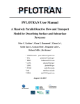
Figure 3.1: A common visualization of EEO models is a directed network graph, with energy sources on the left and
end-use demands on the right. The modeler must specify the specific end-use demands to be met, the technologies of
the system (rectangles), and the inputs and outputs of each (red and green arrows). The circles represent distinct types
of energy carriers.
The most fundamental tenet of the model is the understanding of energy flow, treating all processes as black boxes
that take inputs and produce outputs. Specifically, Temoa does not care about the inner workings of a process, only its
global input and output characteristics. In this vein, the above graphic can be broken down into per-process segments.
For example, the coal power plant takes as input coal and produces electricity, and is subject to various costs (e.g.
variable costs) and constraints (e.g. efficiency) along the way.
7
Temoa Project Documentation, Release 2015-02-03
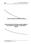
Figure 3.2: The model does not assign any weight to the input or output commodities of a process, just the engineering
characteristics for use of the process itself.
Process: coal_power_plant
coal
Input, (V_FlowIn)
installed capacity
efficiency
install cost
fixed cost
variable cost
emission per unit activity
useful life
loan life
...
Output, (V_FlowOut)
electricity
The modeler defines the processes and engineering characteristics through an amalgam of sets and parameters, described in the next few sections. Temoa then translates these into variables and constraints that an optimizer may then
solve.
3.1 Sets
Table 3.1: List of all Temoa sets with which a modeler might interact. The asterisked (*) elements are automatically
derived by the model and are not user-specifiable.
Set
*
C
C𝑑
C𝑒
C𝑝
* 𝑐
C
I
O
P𝑒
P𝑓
* 𝑜
P
*
V
S
D
*
T
T𝑟
T𝑝
T𝑏
T𝑠
Temoa Name
commodity_all
commodity_demand
commodity_emissions
commodity_physical
commodity_carrier
time_existing
time_future
time_optimize
vintage_all
time_season
time_of_day
tech_all
tech_resource
tech_production
tech_baseload
tech_storage
Data Type
string
string
string
string
string
string
string
Z
Z
Z
Z
string
string
string
string
string
string
string
Short Description
union of all commodity sets
end-use demand commodities
emission commodities (e.g. CO2 , NOx )
general energy forms (e.g. electricity, coal, uranium, oil)
physical energy carriers and end-use demands (C𝑝 ∪ C𝑑 )
alias of C𝑝 ; used in documentation only to mean “input”
alias of C𝑐 ; used in documentation only to mean “output”
model periods before optimization begins
model time scale of interest; the last year is not optimized
model time periods to optimize; (P𝑓 − max(P𝑓 ))
possible tech vintages; (P𝑒 ∪ P𝑜 )
seasonal divisions (e.g. winter, summer)
time-of-day divisions (e.g. morning)
all technologies to be modeled; (𝑇𝑟 ∪ 𝑇𝑝 )
resource extraction techs
techs producing intermediate commodities
baseload electric generators; (𝑇𝑏 ⊂ 𝑇 )
storage technologies; (𝑇𝑠 ⊂ 𝑇 )
Temoa uses two different set notation styles, one for code representation and one that utilizes standard algebraic
notation. For brevity, the mathematical representation uses capital glyphs to denote sets, and small glyphs to represent
items within sets. For example, 𝑇 represents the set of all technologies and 𝑡 represents an item within 𝑇 .
8
Chapter 3. The Math Behind Temoa
Temoa Project Documentation, Release 2015-02-03
The code representation is more verbose than the algebraic version, using full words. This documentation presents
them in an italicized font. The same example of all technologies is represented in the code as tech_all. Note that
regardless, the meanings are identical, with only minor interaction differences inherent to “implementation details.”
Table 1 lists all of the Temoa sets, with both notational schemes.
Their are four basic set “groups” within Temoa: periods, annual “slices”, technology, and energy commodities. The
technological sets contain all the possible energy technologies that the model may build and the commodities sets
contain all the input and output forms of energy that technologies consume and produce. The period and slice sets
merit a slightly longer discussion.
Temoa’s conceptual model of time is broken up into three levels:
• Periods - consecutive blocks of years, marked by the first year in the period. For example, a two-period model
might consist of P𝑓 = {2010, 2015, 2025}, representing the two periods of years from 2010 through 2014, and
from 2015 through 2024.
• Seasonal - Each year may have multiple seasons. For example, winter might demand more heating, while spring
might demand more cooling and transportation.
• Daily - Within a season, a day might have various times of interest. For instance, the peak electrical load might
occur midday in the summer, and a secondary peak might happen in the evening.
There are two specifiable period sets: time_exist (P𝑒 ) and time_future (P𝑓 ). The time_exist set contains
periods before time_future. Its primary purpose is to specify the vintages for capacity that exist prior to the
model optimization. (This is part of Temoa’s answer to what most other efforts model as “residual capacity”.) The
time_future set contains the future periods that the model will optimize. As this set must contain only integers,
Temoa interprets the elements to be the boundaries of each period of interest. Thus, this is an ordered set and Temoa
uses its elements to automatically calculate the length of each optimization period; modelers may exploit this to create
variable period lengths within a model. (To our knowledge, this capability is unique to Temoa.) Temoa “names”
each optimization period by the first year, and makes them easily accessible via the time_optimize set. This final
“period” set is not user-specifiable, but is an exact duplicate of time_future, less the largest element. In the above
example, since P𝑓 = {2010, 2015, 2025}, time_optimize does not contain 2025: P𝑜 = {2010, 2015}.
One final note on periods: rather than optimizing each year within a period individually, Temoa makes a simplifying
assumption that each period contains 𝑛 copies of a single, representative year. Temoa optimizes just this characteristic
year, and only delineates each year within a period through a time-value of money calculation in the objective function.
Figure 3.3 gives a graphical explanation of the annual delineation.
Many EEO efforts need to model sub-annual variations in demand as well. Temoa allows the modeler to subdivide
years into slices, comprised of a season and a time of day (e.g. winter evening). Unlike the periods, there is no
restriction on what labels the modeler may assign to the time_season and time_of_day set elements. There is
similarly no pre-described order, and modeling efforts should not rely on a specific ordering of annual slices.
3.1.1 A Word on Index Ordering
The ordering of the indices is consistent throughout the model to promote an intuitive “left-to-right” description of
each parameter, variable, and constraint set. For example, Temoa’s output commodity flow variable 𝐹 𝑂𝑝,𝑠,𝑑,𝑖,𝑡,𝑣,𝑜
may be described as “in period (𝑝) during season (𝑠) at time of day (𝑑), the flow of input commodity (𝑖) to technology
(𝑡) of vintage (𝑣) generates an output commodity flow (𝑜) of 𝐹 𝑂𝑝,𝑠,𝑑,𝑖,𝑡,𝑣,𝑜 .” For any indexed parameter or variable
within Temoa, our intent is to enable a mental model of a left-to-right arrow-box-arrow as a simple mnemonic to
describe the “input → process → output” flow of energy. And while not all variables, parameters, or constraints have
7 indices, the 7-index order mentioned here (p, s, d, i, t, v, o) is the canonical ordering. If you note any case where,
for example, d comes before s, that is an oversight. In general, if there is an index ordering that does not follow this
rubric, we view that as a bug.
3.1. Sets
9
Temoa Project Documentation, Release 2015-02-03
Figure 3.3: The left graph is of energy, while the right graph is of the annual costs. In other words, the energy used in a
period by a process is the same for all years (with exception for those processes that cease their useful life mid-period).
However, even though the costs incurred will be the same, the time-value of money changes due to the discount-rate.
As the fixed costs of a process are tied to the length of its useful life, those processes that do not fall on a period
boundary require unique time-value multipliers in the objective function.
3.1.2 Deviations from Standard Mathematical Notation
Temoa deviates from standard mathematical notation and set understanding in two ways. The first is that Temoa
places a restriction on the time set elements. Specifically, while most optimization programs treat set elements as
arbitrary labels, Temoa assumes that all elements of the time_existing and time_future sets are integers.
Further, these sets are assumed to be ordered, such that the minimum element is “naught”. For example, if P𝑓 =
{2015, 2020, 2030}, then 𝑃0 = 2015. In other words, the capital P with the naught subscript indicates the first
element in the time_future set. We will explain the reason for this deviation shortly.
The second set of deviations revolves around the use of the Theta superset (Θ). The Temoa code makes heavy use of
sparse sets, for both correctness and efficient use of computational resources. For brevity, and to avoid discussion of
some “implementation details,” we do not enumerate their logical creation here. Instead, we rely on the readers general
understanding of the context. For example, in the sparse creation of the constraints of the Demand constraint class
(explained in Network Constraints and Anatomy of a Constraint), we state simply that the constraint is instantiated
“for all the ⟨𝑝, 𝑠, 𝑑, 𝑑𝑒𝑚⟩ tuples in Θdemand ”. This means that the constraint is only defined for the exact indices for
which the modeler specified end-use demands via the Demand parameter.
Summations also occur in a sparse manner. Take equation (3.1) as an example (described in Decision Variables):
∑︁
ACT𝑝,𝑠,𝑑,𝑡,𝑣 =
FO𝑝,𝑠,𝑑,𝑖,𝑡,𝑣,𝑜
𝐼,𝑂
∀{𝑝, 𝑠, 𝑑, 𝑡, 𝑣} ∈ Θactivity
It defines the Activity variable for every valid combination of ⟨𝑝, 𝑠, 𝑑, 𝑡, 𝑣⟩ as the sum over all inputs and outputs of
the FlowOut variable. A naive implementation of this equation might include nonsensical items in each summation,
like perhaps an input of vehicle miles traveled and an output of sunlight for a wind powered turbine. However,
in this context, summing over the inputs and outputs (𝑖 and 𝑜) implicitly includes only the valid combinations of
⟨𝑝, 𝑠, 𝑑, 𝑖, 𝑡, 𝑣, 𝑜⟩.
3.2 Parameters
10
Chapter 3. The Math Behind Temoa
Temoa Project Documentation, Release 2015-02-03
Table 3.2: List of Temoa parameters with which a modeler might interact. The asterisked (*) elements are automatically derived by the model
and are not user-specifiable.
Parameter
CFD𝑠,𝑑,𝑡
CF𝑠,𝑑,𝑡,𝑣
C2A𝑡,𝑣
FC𝑝,𝑡,𝑣
IC𝑡,𝑣
MC𝑝,𝑡,𝑣
DEM𝑝,𝑐
DDD𝑝,𝑠,𝑑
DSD𝑝,𝑠,𝑑,𝑐
DR𝑡
EFF𝑖,𝑡,𝑣,𝑜
EAC𝑖,𝑡,𝑣,𝑜,𝑒
ELM𝑝,𝑒
ECAP𝑡,𝑣
GDR
GRM
GRS
LLN𝑡,𝑣
LTC𝑝,𝑡,𝑣
MAX𝑝,𝑡
MIN𝑝,𝑡
RSC𝑝,𝑐
SEG𝑠,𝑑
TIS𝑖,𝑡
TOS𝑡,𝑜
*
LA𝑡,𝑣
*
MLL𝑡,𝑣
*
MTL𝑝,𝑡,𝑣
*
LEN𝑝
*
R𝑝
*
TLF𝑝,𝑡,𝑣
Temoa Name
CapacityFactorDefault
CapacityFactor
Capacity2Activity
CostFixed
CostInvest
CostVariable
Demand
DemandDefaultDistribution
DemandSpecificDistribution
DiscountRate
Efficiency
EmissionsActivity
EmissionsLimit
ExistingCapacity
GlobalDiscountRate
GrowthRateMax
GrowthRateSeed
LifetimeLoan
LifetimeTech
MaxCapacity
MinCapacity
ResourceBound
SegFrac
TechInputSplit
TechOutputSplit
LoanAnnualize
ModelLoanLife
ModelTechLife
PeriodLength
PeriodRate
TechLifetimeFrac
Domain
I
I
R+
0
R
R
R
R+
0
I
I
R
R+
0
R
R+
0
R+
0
R
R
R
N
N
R+
0
R+
0
R+
0
I
I
I
R+
0
N
N
N
R
I
Short Description
Technology default capacity factor
Process specific capacity factor
Converts from capacity to activity units
Fixed operations & maintenance cost
Tech-specific investment cost
Variable operations & maintenance cost
End-use demands, by period
Default demand distribution
Demand-specific distribution
Tech-specific interest rate on investment
Tech- and commodity-specific efficiency
Tech-specific emissions rate
Emissions limit by time period
Pre-existing capacity
Global rate used to calculate present cost
Global rate used to calculate present cost
Global rate used to calculate present cost
Tech- and vintage-specific loan term
Tech- and vintage-specific lifetime
maximum tech-specific capacity by period
minimum tech-specific capacity by period
Upper bound on resource use
Fraction of year represented by each (s, d) tuple
Technology input fuel ratio
Technology output fuel ratio
Loan amortization by tech and vintage; based on 𝐷𝑅𝑡
Smaller of model horizon or process loan life
Smaller of model horizon or process tech life
Number of years in period 𝑝
Converts future annual cost to discounted period cost
Fraction of last time period that tech is active
3.2.1 Efficiency
𝐸𝐹 𝐹 𝑖∈𝐶𝑝 ,𝑡∈𝑇,𝑣∈𝑉,𝑜∈𝐶𝑐
As it is the most influential to the rest of the Temoa model, we present the efficiency (𝐸𝐹 𝐹 ) parameter first. Beyond
defining the conversion efficiency of each process, Temoa also utilizes the indices to understand the valid input →
process → output paths for energy. For instance, if a modeler does not specify an efficiency for a 2020 vintage
coal power plant, then Temoa will recognize any mention of a 2020 vintage coal power plant elsewhere as an error.
Generally, if a process is not specified in the efficiency table,1 Temoa assumes it is not a valid process and will provide
the user a warning with pointed debugging information.
1 The efficiency parameter is often referred to as the efficiency table, due to how it looks after even only a few entries in the Pyomo input “dot
dat” file.
3.2. Parameters
11
Temoa Project Documentation, Release 2015-02-03
3.2.2 CapacityFactorDefault
𝐶𝐹 𝐷𝑠∈𝑆,𝑑∈𝐷,𝑡∈𝑇
Where many models assign a capacity factor to a technology class only, Temoa indexes the CapacityFactor
parameter by vintage and time slice as well. This enables the modeler to specify the capacity factor of a process per
season and time of day, as well as recognizing any advances within a sector of technology. However, if the model calls
for a capacity factor that is not 1 (the default), but is the same for all vintages of a technology, this parameter elides
the need to specify all of them.
3.2.3 CapacityFactor
𝐶𝐹 𝑠∈𝑆,𝑑∈𝐷,𝑡∈𝑇,𝑣∈𝑉
In addition to CapacityFactorDefault, there may be cases where different vintages have different capacity factors. This
may be useful, for example, in working with a renewable portfolio, where the amount of a resource is dependent on
the time of year and time of day, and the available technological skill.
3.2.4 Capacity2Activity
𝐶2𝐴𝑡∈𝑇
Capacity and Activity are inherently two different units of measure. Capacity is a unit of energy per time ( 𝑒𝑛𝑒𝑟𝑔𝑦
𝑡𝑖𝑚𝑒 ),
while Activity is a measure of total energy actually emitted (𝑒𝑛𝑒𝑟𝑔𝑦). However, there are times when one needs to
compare the two, and this parameter makes those comparisons more natural. For example, a capacity of 1 GW for one
year works out to an activity of
−6 𝑃
𝑠𝑒𝑐
𝑃𝐽
1𝐺𝑊 · 8, 760 ℎ𝑟
𝑦𝑟 · 3, 600 ℎ𝑟 · 10
𝐺 = 31.536 𝑦𝑟
or
−3 𝑇
1𝐺𝑊 · 8, 760 ℎ𝑟
𝑦𝑟 · 10
𝐺 = 8.75𝑇 𝑊 ℎ
When comparing one capacity to another, the comparison is easy, unit wise. However, when one needs to compare
capacity and activity, how does one reconcile the units? One way to think about the utility of this parameter is in the
context of the question: “How much activity would this capacity create, if used 100% of the time?”
3.2.5 CostFixed
𝐹 𝐶 𝑝∈𝑃,𝑡∈𝑇,𝑣∈𝑉
The CostFixed parameter specifies the fixed cost associated with any process. Fixed costs are those that must be
paid, regardless of the use of a facility. For instance, if the model decides to build a nuclear power plant, even if it
decides not utilize the plant, the model must pay the fixed costs. These are in addition to the loan, so once the loan is
paid off, these costs are still incurred every year the process exists.
Temoa’s default objective function assumes the modeler has specified this parameter in units of currency per unit
𝐶𝑈 𝑅
capacity ( 𝑈 𝑛𝑖𝑡𝐶𝑎𝑝
).
3.2.6 CostInvest
𝐼𝐶 𝑡∈𝑇,𝑣∈𝑃
12
Chapter 3. The Math Behind Temoa
Temoa Project Documentation, Release 2015-02-03
The CostInvest parameter specifies the cost of the loan. Unlike the CostFixed and CostVariable parameters, CostInvest only applies to vintages of technologies within the model optimization horizon (P𝑜 ). Like
CostFixed, CostInvest is specified in units of currency per unit of capacity and is only used in the default
𝐶𝑈 𝑅
).
objective function ( 𝑈 𝑛𝑖𝑡𝐶𝑎𝑝
3.2.7 CostVariable
𝑀 𝐶 𝑝∈𝑃,𝑡∈𝑇,𝑣∈𝑉
The CostVariable parameter is a measure of the cost of a unit of activity of an installed process. It is specified as
a unit of currency per a unit of activity and is only used in the default objective function.
3.2.8 Demand
𝐷𝐸𝑀 𝑝∈𝑃,𝑐∈𝐶 𝑑
The Demand parameter allows the modeler to define the total end-use demand levels for all periods. In combination
with the Efficiency parameter, this parameter is the most important because without it, the rest of model has no
incentive to build anything. In terms of the system map, this parameter specifies the far right.
To specify the distribution of demand, look to the DemandDefaultDistribution (DDD) and
DemandSpecificDistribution (DSD) parameters.
As a historical note, this parameter was at one time also indexed by season and time of day, allowing modelers to
specify exact demands for every time slice. However, while extremely flexible, this proved too tedious to maintain for
any data set of appreciable size. Thus, we implemented the DDD and DSD parameters.
3.2.9 DemandDefaultDistribution
𝐷𝐷𝐷𝑠∈𝑆,𝑑∈𝐷
By default, Temoa assumes that end-use demands (Demand) are evenly distributed throughout a year. In other words,
the Demand will be apportioned by the SegFrac parameter via:
EndUseDemand𝑠,𝑑,𝑐 = 𝑆𝑒𝑔𝐹 𝑟𝑎𝑐𝑠,𝑑 · 𝐷𝑒𝑚𝑎𝑛𝑑𝑝,𝑐
Temoa enables this default action by automatically setting DDD equivalent to SegFrac for all seasons and times of
day. If a modeler would like a different default demand distribution, the modeler must specify any indices of the DDD
parameter. Like the SegFrac parameter, the sum of DDD must be 1.
3.2.10 DemandSpecificDistribution
𝐷𝑆𝐷𝑠∈𝑆,𝑑∈𝐷,𝑐∈𝐶 𝑑
If there is an end-use demand that does not follow the default distribution – for example, heating or cooling in the
summer or winter – the modeler may specify as much with this parameter. Like SegFrac and DemandDefaultDistribution, the sum of DSD for each 𝑐 must be 1. If the modeler does not define DSD for a season, time of day, and demand
commodity, Temoa automatically populates this parameter according to DDD. It is this parameter that is actually
multiplied by the Demand parameter in the Demand constraint.
3.2. Parameters
13
Temoa Project Documentation, Release 2015-02-03
3.2.11 DiscountRate
𝐷𝑅𝑡∈𝑇
In addition to the GlobalDiscountRate, a modeler may also specify a technology-specific discount rate. If not
specified, this rate defaults to the GDR to represent a social discount rate.
3.2.12 EmissionActivity
𝐸𝐴𝐶 𝑒∈𝐶𝑒 ,{𝑖,𝑡,𝑣,𝑜}∈Θefficiency
Temoa currently has two methods for enabling a process to produce an output: the Efficiency parameter, and
the EmissionActivity parameter. Where the Efficiency parameter defines the amount of output energy a
process produces per unit of input, the EmissionActivity parameter allows for secondary outputs. As the name
suggests, this parameter was originally intended to account for emissions per unit activity, but it more accurately
describes parallel activity. For the time being, it is restricted to emissions accounting (by the 𝑒 ∈ 𝐶 𝑒 set restriction),
but an item on the Temoa TODO list is to upgrade the use of this parameter. For instance, Temoa does not currently
provide an easy avenue to model a dual-function process, such as a combined heat and power plant.
3.2.13 EmissionLimit
𝐸𝐿𝑀 𝑝∈𝑃,𝑒∈𝐶 𝑒
The EmissionLimit parameter is fairly self explanatory, ensuring that Temoa finds a solution that fits within the
modeler-specified limit of emission 𝑒 in time period 𝑝.
3.2.14 ExistingCapacity
𝐸𝐶𝐴𝑃 𝑡∈𝑇,𝑣∈P𝑒
In contrast to some competing models, technologies in Temoa can have vintage-specific characteristics within the same
period. Thus, Temoa treats existing technological capacity as processes, requiring all of the engineering characteristics
of a standard process. This is Temoa’s answer to what some call “residual capacity.”
3.2.15 GlobalDiscountRate
𝐺𝐷𝑅
In financial circles, the value of money is dependent on when it was measured. There is no method to measure the
absolute value of a currency, but there are generally accepted relative rates for forecasting and historical purposes.
Temoa uses the same general concept, that the future value (FV) of a sum of currency is related to the net present value
(NPV) via the formula:
FV = NPV · (1 + 𝐺𝐷𝑅)𝑛
where 𝑛 is in years. This parameter is only used in Temoa’s objective function.
3.2.16 LifetimeLoan
𝐿𝐿𝑁 𝑡∈𝑇,𝑣∈𝑃
Temoa differs from many EEO models by giving the modeler the ability to separate the loan lifetime from the useful
life of the technology. This parameter specifies the length of the loan associated with investing in a process, in years.
If not specified, the default is 30 years.
14
Chapter 3. The Math Behind Temoa
Temoa Project Documentation, Release 2015-02-03
3.2.17 LifetimeTech
𝐿𝑇 𝐶 𝑝∈𝑃,𝑡∈𝑇,𝑣∈𝑉
Similar to LifetimeLoan, this parameter specifies the total useful life of technology, years. If not specified, the default
is 10 years.
3.2.18 MaxCapacity
𝑀 𝐴𝑋 𝑝∈𝑃,𝑡∈𝑇
The MaxCapacity parameter enables a modeler to ensure that a certain technology is constrained to an upper bound.
The enforcing constraint ensures that the max total capacity (summed across vintages) of a technology class is under
this maximum. That is, all active vintages are constrained. This parameter is used only in the maximum capacity
constraint.
3.2.19 MinCapacity
𝑀 𝐼𝑁 𝑝∈𝑃,𝑡∈𝑇
The MinCapacity parameter is analogous to the maximum capacity parameter, except that it specifies the minimum
capacity for which Temoa must ensure installation.
3.2.20 ResourceBound
𝑅𝑆𝐶 𝑝∈𝑃,𝑐∈𝐶𝑝
This parameter allows the modeler to specify resources to constrain per period. Note that a constraint in one period
does not relate to any other periods. For instance, if the modeler specifies a limit in period 1 and does not specify a
limit in period 2, then the model may use as much of that resource as it would like in period 2.
3.2.21 SegFrac
𝑆𝐸𝐺𝑠∈𝑆,𝑑∈𝐷
The SegFrac parameter specifies the fraction of the year represented by each combination of season and time of day.
The sum of all combinations within SegFrac must be 1, representing 100% of a year.
3.2.22 TechInputSplit
𝑆𝑃 𝐿𝑖∈𝐶𝑝 ,𝑡∈𝑇
Some technologies have a single output but have multiple input fuels. For the sake of modeling, certain technologies
require a fixed apportion of relative input. See the TechOutputSplit constraint for the implementation concept.
3.2.23 TechOutputSplit
𝑆𝑃 𝐿𝑡∈𝑇,𝑜∈𝐶𝑐
Some technologies have a single input fuel but have multiple output forms of energy. For the sake of modeling, certain
technologies require a fixed apportion of relative output. For example, an oil refinery might have an input energy of
crude oil, and the modeler wants to ensure that its output is 70% diesel and 30% gasoline. See the TechOutputSplit
constraint for the implementation details.
3.2. Parameters
15
Temoa Project Documentation, Release 2015-02-03
3.2.24 *LoanAnnualize
𝐿𝐴𝑡∈𝑇,𝑣∈𝑃
This is a model-calculated parameter based on the process-specific loan length (it’s indices are the same as the
LifetimeLoan parameter), and process-specific discount rate (the DiscountRate parameter). It is calculated
via the formula:
𝐷𝑅𝑡,𝑣
𝐿𝐴𝑡,𝑣 =
−
1 − (1 + 𝐷𝑅𝑡,𝑣 ) 𝐿𝐿𝑁𝑡,𝑣
∀{𝑡, 𝑣} ∈ ΘCostInvest
3.2.25 *PeriodLength
𝐿𝐸𝑁 𝑝∈𝑃
Given that the modeler may specify arbitrary period boundaries, this parameter specifies the number of years contained
in each period. The final year is the largest element in time_future which is specifically not included in the list
of periods in time_optimize (P𝑜 ). The length calculation for each period then exploits the fact that the time sets
are ordered:
LET boundaries = sorted(P𝑓 )
LET I(p) = index of p in boundaries
∴
𝐿𝐸𝑁 𝑝 = boundaries[𝐼(𝑝) + 1] − 𝑝
∀𝑝 ∈ 𝑃
The first line creates a sorted array of the period boundaries, called boundaries. The second line defines a function I
that finds the index of period 𝑝 in boundaries. The third line then defines the length of period 𝑝 to be the number of
years between period 𝑝 and the next period. For example, if P𝑓 = {2015, 2020, 2030, 2045}, then boundaries would
be [2015, 2020, 2030, 2045]. For 2020, I(2020) would return 2. Similarly, boundaries[ 3 ] = 2030. Then,
𝐿𝐸𝑁 2020 = boundaries[𝐼(2020) + 1] − (2020)
= boundaries[2 + 1] − 2020
= boundaries[3] − 2020
= 2030 − 2020
= 10
Note that LEN is only defined for elements in P𝑜 , and is specifically not defined for the final element in P𝑓 .
3.2.26 *PeriodRate
𝑅𝑝∈𝑃
Temoa optimizes a single characteristic year within a period, and differentiates the 𝑛 copies of that single year solely by
the appropriate discount factor. Rather than calculating the same summation for every technology and vintage within
a period, we calculate it once per period and lookup the sum as necessary during the objective function generation.
The formula is the sum of discount factors corresponding to each year within a period:
𝐿𝐸𝑁 𝑝
𝑅𝑝 =
1
∑︁
(𝑃0 −𝑝−𝑦)
𝑦=0
(1 + 𝐺𝐷𝑅)
∀𝑝 ∈ 𝑃
16
Chapter 3. The Math Behind Temoa
Temoa Project Documentation, Release 2015-02-03
Note that this parameter is the implementation of the single “characteristic year” optimization per period concept
discussed in the Sets section.
3.2.27 *TechLifeFrac
𝑇 𝐿𝐹 𝑝∈𝑃,𝑡∈𝑇,𝑣∈𝑉
The modeler may specify a useful lifetime of a process such that the process will be decommissioned part way through
a period. Rather than attempt to delineate each year within that final period, Temoa makes the choice to average the
total output of the process over the entire period but limit the available capacity and output of the decommissioning
process by the ratio of how long through the period the process is active. This parameter is that ratio, formally defined
as:
𝑇 𝐿𝐹𝑝,𝑡,𝑣 =
𝑣 + 𝐿𝑇 𝐶𝑡,𝑣 − 𝑝
𝐿𝐸𝑁𝑝
∀{𝑝, 𝑡, 𝑣} ∈ ΘActivity by PTV |
𝑣 + 𝐿𝑇 𝐶𝑡,𝑣 ∈
/ 𝑃,
𝑣 + 𝐿𝑇 𝐶𝑡,𝑣 ≤ 𝑚𝑎𝑥(𝐹 ),
𝑝 = 𝑚𝑎𝑥(𝑃 |𝑝 < 𝑣 + 𝐿𝑇 𝐶𝑡,𝑣 )
Note that this parameter is defined over the same indices as CostVariable – the active periods for each process
⟨𝑝, 𝑡, 𝑣⟩. As an example, if a model has 𝑃 = {2010, 2012, 2020, 2030}, and a process ⟨𝑡, 𝑣⟩ = ⟨𝑐𝑎𝑟, 2010⟩ has a
useful lifetime of 5 years, then this parameter would include only the first two activity indices for the process. Namely,
𝑝 ∈ {2010, 2012} as ⟨𝑝, 𝑡, 𝑣⟩ ∈ {⟨2010, 𝑐𝑎𝑟, 2010⟩ , ⟨2012, 𝑐𝑎𝑟, 2010⟩}. The values would be 𝑇 𝐿𝐹 2010,𝑐𝑎𝑟,2010 = 1,
and 𝑇 𝐿𝐹 2012,𝑐𝑎𝑟,2010 = 83 .
In combination with the PeriodRate parameter, this parameter is used to implement the “single characteristic year”
simplification. Specifically, instead of trying to account for partial period decommissioning, Temoa assumes that
processes can only produce TechLifeFrac of their installed capacity.
3.3 Variables
Table 3.3: Temoa’s Main Variables
The
Variable
𝐹 𝐼𝑝,𝑠,𝑑,𝑖,𝑡,𝑣,𝑜
𝐹 𝑂𝑝,𝑠,𝑑,𝑖,𝑡,𝑣,𝑜
𝐴𝐶𝑇𝑝,𝑠,𝑑,𝑡,𝑣
𝐶𝐴𝑃𝑡,𝑣
𝐶𝐴𝑃 𝐴𝑉 𝐿𝑝,𝑡
Temoa Name
Domain Short Description
V_FlowIn
R+
Commodity flow into a tech to produce a given output
0
+
V_FlowOut
R0
Commodity flow out of a tech based on a given input
V_Activity
R+
Total tech commodity production in each (s, d) tuple
0
V_Capacity
R+
Required tech capacity to support associated activity
0
V_CapacityAvailableR+
The Capacity of technology 𝑡 available in period 𝑝
0
ByPeriodAndTech
most fundamental variables in the Temoa formulation are 𝐹 𝑙𝑜𝑤𝐼𝑛 and 𝐹 𝑙𝑜𝑤𝑂𝑢𝑡. They describe the commodity
flows into and out of a process in a given time slice. They are related through the ProcessBalance constraint (3.5),
which in essence, guarantees the conservation of energy for each process.
The Activity variable is defined as the sum over all inputs and outputs of a process in a given time slice (see equation
(3.1)). At this time, one potential “gotcha” is that for a process with multiple inputs or outputs, there is no attempt to
reconcile energy units: Temoa assumes all inputs are comparable, and as no understanding of units. The onus is on
the modeler to ensure that all inputs and outputs have similar units.2
2
There is an open ticket to address the lack of unit awareness in Temoa. See issue 5 in our issue tracker.
3.3. Variables
17
Temoa Project Documentation, Release 2015-02-03
The Capacity variable is used in the default objective function as the amount of capacity of a process to build. It is
indexed for each process, and Temoa constrains the Capacity variable to at least be able to meet the Activity of that
process in all time slices in which it is active (3.2).
Finally, CapacityAvailableByPeriodAndTech is a convenience variable that is not strictly necessary, but used where
the individual vintages of a technology are not warranted (e.g. in calculating the maximum or minimum total capacity
allowed in a given time period).
We explain the equations governing these variables the Constraints section.
3.4 Constraints
There are 4 main equations that govern the flow of energy through the model network. The DemandConstraint ensures
that the supply meets demand in every time slice. For each process, the ProcessBalance ensures at least as much energy
enters a process as leaves it (conservation of energy at the process level). Between processes, the CommodityBalance
ensures that at least as much of a commodity is generated as is demanded by other process inputs.
In combination, those three constraints ensure the flow of energy through the system. The final calculation, the
objective function, is what puts a monetary cost to the actions dictated by the model.
The rest of this section defines each model constraint, with a rationale for existence. We use the implementationspecific names for the constraints as both an artifact of our documentation generation process, and to highlight the
organization of the functions within the actual code. They are listed roughly in order of importance.
3.4.1 Decision Variables
These first two constraints elucidate the relationship among decision variables in the model. There is some overlap
with the rest of the constraints, but these are unique enough to warrant special attention to a Temoa modeler.
temoa_rules.Activity_Constraint(M, p, s, d, t, v)
The Activity constraint defines the Activity convenience variable. The Activity variable is mainly used in the
objective function to calculate the cost associated with use of a technology. In English, this constraint states that
“the activity of a process is the sum of its outputs.”
There is one caveat to keep in mind in regards to the Activity variable: if there is more than one output, there
is currently no attempt by Temoa to convert to a common unit of measurement. For example, common measurements for heat include mass of steam at a given temperature, or total BTUs, while electricity is generally
measured in a variant of watt-hours. Reconciling these units of measurement, as for example with a cogeneration
plant, is currently left as an accounting exercise for the modeler.
∑︁
ACT𝑝,𝑠,𝑑,𝑡,𝑣 =
FO𝑝,𝑠,𝑑,𝑖,𝑡,𝑣,𝑜
(3.1)
𝐼,𝑂
∀{𝑝, 𝑠, 𝑑, 𝑡, 𝑣} ∈ Θactivity
temoa_rules.Capacity_Constraint(M, p, s, d, t, v)
Temoa’s definition of a process’ capacity is the total size of installation required to meet all of that process’
demands. The Activity convenience variable represents exactly that, so the calculation on the left hand side of
the inequality is the maximum amount of energy a process can produce in the time slice <s,d>.
(CFP𝑡,𝑣 · C2A𝑡 · SEG𝑠,𝑑 · TLF𝑝,𝑡,𝑣 ) · CAP𝑡,𝑣 ≥ ACT𝑝,𝑠,𝑑,𝑡,𝑣
(3.2)
∀{𝑝, 𝑠, 𝑑, 𝑡, 𝑣} ∈ Θactivity
18
Chapter 3. The Math Behind Temoa
Temoa Project Documentation, Release 2015-02-03
temoa_rules.CapacityAvailableByPeriodAndTech_Constraint(M, p, t)
The CAPAVL variable is nominally for reporting solution values, but is also used in the Max and Min constraint
calculations. For any process with an end-of-life (EOL) on a period boundary, all of its capacity is available
for use in all periods in which it is active (the process’ TLF is 1). However, for any process with an EOL that
falls between periods, Temoa makes the simplifying assumption that the available capacity from the expiring
technology is available through the whole period, but only as much percentage as its lifespan through the period.
For example, if a process expires 3 years into an 8 year period, then only 38 of the installed capacity is available
for use throughout the period.
∑︁
CAPAVL𝑝,𝑡 =
𝑇 𝐿𝐹 𝑝,𝑡,𝑣 · CAP
(3.3)
𝑉
∀𝑝 ∈ P𝑜 , 𝑡 ∈ 𝑇
3.4.2 Network Constraints
These three constraints define the core of the Temoa model. Together, they create the algebraic network. The Demand
constraint drives the “right side” of the energy system map, the ProcessBalance constraint ensures flow through a
process, and the CommodityBalance constraint ensures flow between processes.
temoa_rules.Demand_Constraint(M, p, s, d, dem)
The Demand constraint drives the model. This constraint ensures that supply at least meets the demand specified
by the Demand parameter in all periods and slices, by ensuring that the sum of all the demand output commodity
(𝑐) generated by FO must meet the modeler-specified demand, in each time slice.
∑︁
FO𝑝,𝑠,𝑑,𝑖,𝑡,𝑣,𝑑𝑒𝑚 ≥ 𝐷𝐸𝑀 𝑝,𝑑𝑒𝑚 · 𝐷𝑆𝐷𝑠,𝑑,𝑑𝑒𝑚
(3.4)
𝐼,𝑇,𝑉
∀{𝑝, 𝑠, 𝑑, 𝑑𝑒𝑚} ∈ Θdemand
Note that the validity of this constraint relies on the fact that the 𝐶 𝑑 set is distinct from both 𝐶 𝑒 and 𝐶 𝑝 . In
other words, an end-use demand must only be an end-use demand. Note that if an output could satisfy both an
end-use and internal system demand, then the output from FO would be double counted.
Note also that this constraint is an inequality, not a strict equality. “Supply must meet or exceed demand.”
Like with the ProcessBalance constraint, if this constraint is not binding, it may be a clue that the model under
inspection could be more tightly specified and could have at least one input data anomaly.
temoa_rules.ProcessBalance_Constraint(M, p, s, d, i, t, v, o)
The ProcessBalance constraint is one of the most fundamental constraints in the Temoa model. It defines the
basic relationship between the energy entering a process (FI) and the energy leaving a processing (FO). This
constraint sets the FlowOut variable, upon which all other constraints rely.
Conceptually, this constraint treats every process as a “black box,” caring only about the process efficiency. In
other words, the amount of energy leaving a process cannot exceed the amount coming in.
Note that this constraint is an inequality – not a strict equality. In most sane cases, the optimal solution should
make this constraint and supply should exactly meet demand. If this constraint is not binding, it is likely a clue
that the model under inspection could be more tightly specified and has at least one input data anomaly.
FO𝑝,𝑠,𝑑,𝑖,𝑡,𝑣,𝑜 ≤ 𝐸𝐹 𝐹𝑖,𝑡,𝑣,𝑜 · FI𝑝,𝑠,𝑑,𝑖,𝑡,𝑣,𝑜
(3.5)
∀{𝑝, 𝑠, 𝑑, 𝑖, 𝑡, 𝑣, 𝑜} ∈ Θvalid process flows
3.4. Constraints
19
Temoa Project Documentation, Release 2015-02-03
temoa_rules.CommodityBalance_Constraint(M, p, s, d, c)
Where the Demand constraint (3.4) ensures that end-use demands are met, the CommodityBalance constraint
ensures that the internal system demands are met. That is, this is the constraint that ties the output of one process
to the input of another. At the same time, this constraint also conserves energy between process. (But it does
not account for transmission loss.) In this manner, it is a corollary to both the ProcessBalance (3.5) and Demand
(3.4) constraints.
∑︁
∑︁
FO𝑝,𝑠,𝑑,𝑖,𝑡,𝑣,𝑐 ≥
FI𝑝,𝑠,𝑑,𝑐,𝑡,𝑣,𝑜
(3.6)
𝐼,𝑇,𝑉
𝑇,𝑉,𝑂
∀{𝑝, 𝑠, 𝑑, 𝑐} ∈ Θcommodity balance
3.4.3 Physical and Operational Constraints
These three constraints fine-tune the algebraic map created by the three previous constraints, based on various physical
and operational real-world phenomena.
temoa_rules.BaseloadDiurnal_Constraint(M, p, s, d, t, v)
There exists within the electric sector a class of technologies whose thermodynamic properties are impossible
to change over a short period of time (e.g. hourly or daily). These include coal and nuclear power plants, which
take weeks to bring to an operational state, and similarly require weeks to fully shut down. Temoa models
this behavior by forcing technologies in the tech_baseload set to maintain a constant output for all daily
slices. Note that this allows the model to (not) use a baseload process in a season, and only applies over the
time_of_day set.
Ideally, this constraint would not be necessary, and baseload processes would simply not have a 𝑑 index. However, implementing the more efficient functionality is currently on the Temoa TODO list.
𝑆𝐸𝐺𝑠,𝐷0 · ACT𝑝,𝑠,𝑑,𝑡,𝑣 = 𝑆𝐸𝐺𝑠,𝑑 · ACT𝑝,𝑠,𝐷0 ,𝑡,𝑣
(3.7)
∀{𝑝, 𝑠, 𝑑, 𝑡, 𝑣} ∈ Θbaseload
temoa_rules.DemandActivity_Constraint(M, p, s, d, t, v, dem, s_0, d_0)
For end-use demands, it is unreasonable to let the optimizer only allow use in a single time slice. For instance,
if household A buys a natural gas furnace while household B buys an electric furnace, then both units should
be used throughout the year. Without this constraint, the model might choose to only use the electric furnace
during the day, and the natural gas furnace during the night.
This constraint ensures that the ratio of a process activity to demand is constant for all time slices. Note that if a
demand is not specified in a given time slice, or is zero, then this constraint will not be considered for that slice
and demand. This is transparently handled by the Θ superset.
∑︁
∑︁
𝐷𝐸𝑀𝑝,𝑠,𝑑,𝑑𝑒𝑚 ·
FO𝑝,𝑠0 ,𝑑0 ,𝑖,𝑡,𝑣,𝑑𝑒𝑚 = 𝐷𝐸𝑀𝑝,𝑠0 ,𝑑0 ,𝑑𝑒𝑚 ·
FO𝑝,𝑠,𝑑,𝑖,𝑡,𝑣,𝑑𝑒𝑚
(3.8)
𝐼
𝐼
∀{𝑝, 𝑠, 𝑑, 𝑡, 𝑣, 𝑑𝑒𝑚, 𝑠0 , 𝑑0 } ∈ Θdemand activity
temoa_rules.Storage_Constraint(M, p, s, i, t, v, o)
Temoa’s algorithm for storage is to ensure that the amount of energy entering and leaving a storage technology
is balanced over the course of a day, accounting for the conversion efficiency of the storage process. This
constraint relies on the assumption that the total amount of storage-related energy is small compared to the
amount of energy required by the system over a season. If it were not, the algorithm would have to account
20
Chapter 3. The Math Behind Temoa
Temoa Project Documentation, Release 2015-02-03
for season-to-season transitions, which would require an ordering of seasons within the model. Currently, each
slice is completely independent of other slices.
∑︁
(𝐸𝐹 𝐹𝑖,𝑡,𝑣,𝑜 · FI𝑝,𝑠,𝑑,𝑖,𝑡,𝑣,𝑜 − FO𝑝,𝑠,𝑑,𝑖,𝑡,𝑣,𝑜 ) = 0
(3.9)
𝐷
∀{𝑝, 𝑠, 𝑖, 𝑡, 𝑣, 𝑜} ∈ Θstorage
3.4.4 Objective Function
temoa_rules.TotalCost_rule(M)
Using the Activity and Capacity variables, the Temoa objective function calculates the costs associated
with supplying the system with energy, under the assumption that all costs are paid for through loans (rather
than with lump-sum sales). This implementation sums up all the costs incurred by the solution, and is defined
as 𝐶𝑡𝑜𝑡 = Cloans + Cfixed + Cvariable . Similarly, each term on the right-hand side is merely a summation of the
costs incurred, multiplied by an annual discount factor to calculate the discounted cost in year P0 .
]︂
)︂
∑︁ (︂[︂
(1 + 𝐺𝐷𝑅)𝑃0 −𝑣+1 · (1 − (1 + 𝐺𝐷𝑅)−𝑀 𝐿𝐿𝑡,𝑣 )
· CAP𝑡,𝑣
𝐶𝑙𝑜𝑎𝑛𝑠 =
𝐼𝐶𝑡,𝑣 · 𝐿𝐴𝑡,𝑣 ·
𝐺𝐷𝑅
𝑡,𝑣∈Θ𝐼𝐶
𝐶𝑓 𝑖𝑥𝑒𝑑 =
∑︁
(︂[︂
𝐹 𝐶𝑝,𝑡,𝑣 ·
𝑝,𝑡,𝑣∈Θ𝐹 𝐶
]︂
)︂
(1 + 𝐺𝐷𝑅)𝑃0 −𝑝+1 · (1 − (1 + 𝐺𝐷𝑅)−𝑀 𝐿𝐿𝑡,𝑣 )
· CAP𝑡,𝑣
𝐺𝐷𝑅
𝐶𝑣𝑎𝑟𝑖𝑎𝑏𝑙𝑒 =
∑︁
(𝑀 𝐶𝑝,𝑡,𝑣 · 𝑅𝑝 · ACT𝑡,𝑣 )
𝑝,𝑡,𝑣∈Θ𝑉 𝐶
In the last sub-equation, 𝑅𝑝 is the equivalent operation to the inner summation of the other two sub-equations.
The difference is that where the inner summations specifically account for the fixed and loan costs of partialperiod processes, the activity is constant for all years within a period. There is thus no need to calculate the
time-value of money factor for each process, and instead, 𝑅𝑝 is calculated once for each period, as a pseudoparameter. While this amounts to little more than an efficiency of model generation, it is pedagogically significant in that it highlights the fact that Temoa optimizes only a single characteristic year within each period.
3.4.5 User-Specific Constraints
The constraints provided in this section are not required for proper system operation, but allow the modeler some
further degree of system specification.
temoa_rules.ExistingCapacity_Constraint(M, t, v)
Temoa treats residual capacity from before the model’s optimization horizon as regular processes, that require
the same parameter specification in the data file as do new vintage technologies (e.g. entries in the efficiency
table), except the CostInvest parameter. This constraint sets the capacity of processes for model periods that
exist prior to the optimization horizon to user-specified values.
CAP𝑡,𝑣 = 𝐸𝐶𝐴𝑃𝑡,𝑣
(3.10)
∀{𝑡, 𝑣} ∈ Θexisting
temoa_rules.EmissionLimit_Constraint(M, p, e)
A modeler can track emissions through use of the commodity_emissions set and EmissionActivity
3.4. Constraints
21
Temoa Project Documentation, Release 2015-02-03
parameter. The 𝐸𝐴𝐶 parameter is analogous to the efficiency table, tying emissions to a unit of activity. The
EmissionLimit constraint allows the modeler to assign an upper bound per period to each emission commodity.
∑︁
(𝐸𝐴𝐶𝑒,𝑖,𝑡,𝑣,𝑜 · FO𝑝,𝑠,𝑑,𝑖,𝑡,𝑣,𝑜 ) ≤ 𝐸𝐿𝑀𝑝,𝑒
(3.11)
𝐼,𝑇,𝑉,𝑂|𝑒,𝑖,𝑡,𝑣,𝑜∈𝐸𝐴𝐶𝑖𝑛𝑑
∀{𝑝, 𝑒} ∈ 𝐸𝐿𝑀𝑖𝑛𝑑
temoa_rules.MaxCapacity_Constraint(M, p, t)
The MinCapacity and MaxCapacity constraints set limits on the what the model is allowed to (not) have available
of a certain technology. Note that the indices for these constraints are period and tech_all, not tech and vintage.
(3.12)
CAPAVL𝑝,𝑡 ≥ 𝑀 𝐼𝑁𝑝,𝑡
∀{𝑝, 𝑡} ∈ ΘMinCapacity parameter
(3.13)
CAPAVL𝑝,𝑡 ≤ 𝑀 𝐴𝑋𝑝,𝑡
∀{𝑝, 𝑡} ∈ ΘMaxCapacity parameter
temoa_rules.ResourceExtraction_Constraint(M, p, r)
The ResourceExtraction constraint allows a modeler to specify an annual limit on the amount of a particular
resource Temoa may use in a period.
∑︁
FO𝑝,𝑠,𝑑,𝑖,𝑡,𝑣,𝑐 ≤ 𝑅𝑆𝐶𝑝,𝑐
(3.14)
𝑆,𝐷,𝐼,𝑡∈𝑇 𝑟 ,𝑉
∀{𝑝, 𝑐} ∈ Θresource bound parameter
temoa_rules.TechInputSplit_Constraint(M, p, s, d, i, t, v)
Some processes make a single output from multiple inputs. A subset of these processes have a constant ratio of
inputs. See TechOutputSplit_Constraint for the analogous math reasoning.
temoa_rules.TechOutputSplit_Constraint(M, p, s, d, t, v, o)
Some processes take a single input and make multiple outputs. A subset of these processes have a constant ratio
of outputs relative to their input. The most canonical example is that of an oil refinery. Crude oil is composed of
many different types of hydrocarbons, and the refinery process exploits the fact that they each have a different
boiling point. The amount of each type of product that a refinery produces is thus directly related to the makeup
of the crude oil input.
The TechOutputSplit constraint assumes that the input to any process of interest has a constant ratio output. For
example, a hypothetical (and highly simplified) refinery might have a crude oil input that only contains 4 parts
diesel, 3 parts gasoline, and 2 parts kerosene. The relative ratios to the output then are:
𝑑=
4
9
· total output,
𝑔=
3
9
· total output,
𝑘=
2
9
· total output
In constraint in set notation is:
∑︁
FO𝑝,𝑠,𝑑,𝑖,𝑡,𝑣,𝑜 = 𝑆𝑃 𝐿𝑡,𝑜 · ACT𝑝,𝑠,𝑑,𝑡,𝑣
(3.15)
𝐼
∀{𝑝, 𝑠, 𝑑, 𝑡, 𝑣, 𝑜} ∈ Θsplit output
22
Chapter 3. The Math Behind Temoa
Temoa Project Documentation, Release 2015-02-03
3.5 General Caveats
Temoa does not currently provide an easy avenue to track multiple concurrent energy flows through a process. Consider
a cogeneration plant. Where a conventional power plant might simply emit excess heat as exhaust, a cogeneration
plant harnesses some or all of that heat for heating purposes, either very close to the plant, or generally as hot water
for district heating. Temoa’s flow variables can track both flows through a process, but each flow will have its own
1
efficiency from the Efficiency parameter. This implies that to produce 1 unit of electricity will require 𝑒𝑙𝑐𝑒𝑓
𝑓 units of
input. At the same time, to produce 1 unit of heat will require units of input energy, and to produce both output units
of heat and energy, both flows must be active, and the desired activity will be double-counted by Temoa.
To model a parallel output device (c.f., a cogeneration plant), the modeler must currently set up the process with the
TechInputSplit and TechOutputSplit parameters, appropriately adding each flow to the Efficiency parameter and accounting for the overall process efficiency through all flows.
3.5. General Caveats
23
Temoa Project Documentation, Release 2015-02-03
24
Chapter 3. The Math Behind Temoa
CHAPTER
FOUR
THE TEMOA COMPUTATIONAL IMPLEMENTATION
We have implemented Temoa within an algebraic modeling environment (AME). AMEs provide both a convenient
avenue to describe mathematical optimization models for a computational context, and allow for abstract model1
formulations [Kallrath04]. In contrast to describing a model in a formal computer programming language like C or
Java, AMEs generally have syntax that directly translates to standard mathematical notation. Consequently, models
written in AMEs are more easily understood by a wider variety of people. Further, by allowing abstract formulations,
a model written with an AME may be used with many different input data sets.
Three well-known and popular algebraic modeling environments are the General Algebraic Modeling System (GAMS)
[BrookeRosenthal03], AMPL [FourerGayKernighan87], and GNU MathProg [Makhorin00]. All three environments
provide concise syntax that closely resembles standard (paper) notation. We decided to implement Temoa within a
recently developed AME called Python Optimization Modeling Objects (Pyomo).
Pyomo provides similar functionality to GAMS, AMPL, and MathProg, but is open source and written in the Python
scripting language. This has two general consequences of which to be aware:
• Python is a scripting language; in general, scripts are an order of magnitude slower than an equivalent compiled
program.
• Pyomo provides similar functionality, but because of its Python heritage, is much more verbose than GAMS,
AMPL, or MathProg.
It is our view that the speed penalty of Python as compared to compiled languages is inconsequential in the face
of other large resource bottle necks, so we omit any discussion of it as an issue. However, the “boiler-plate” code
(verbosity) overhead requires some discussion. We discuss this in the Anatomy of a Constraint.
4.1 File Structure
The Temoa model code is split into 5 main files:
• temoa_model.py - contains the overall model definition, defining the various sets, parameters, variables,
and equations of the Temoa model. Peruse this file for a high-level overview of the model.
• temoa_rules.py - mainly contains the rule implementations. That is, this file implements the objective
function, internal parameters, and constraint logic. Where temoa_model provides the high-level overview,
this file provides the actual equation implementations.
• temoa_lib.py - mainly contains meta functions for the model. For instance, Temoa makes heavy use of
sparse sets, and temoa_lib contains the functions that create those sparse sets. This file also contains various
error checking routines (so that their logic does not clutter the implementations in temoa_rules) as well as
the logic that handles the command line interaction.
1 In contrast to a ‘concrete’ model, an abstract algebraic formulation describes the general equations of the model, but requires modeler-specified
input data before it can compute any results.
25
Temoa Project Documentation, Release 2015-02-03
• temoa_graphviz.py - Currently Temoa’s sole visualizations are generated through Graphviz. This file
contains the various Graphviz-specific graph generation routines.
• temoa_stochastic.py - contains the PySP required alterations to the deterministic model for use in a
stochastic model. Specifically, Temoa only needs one additional constraint class in order to partition the calculation of the objective function per period.
If you are working with the release snapshot of the Temoa model, then you will only see one file, temoa.py. This
file is actually a compressed archive (in ZIP format) containing these 5 files, and may be manipulated with standard
utilities (e.g. PKZIP, WinZip, Info-ZIP). (Due to implementation details, be careful uncompressing the archive as it is
analogous to a “Tarbomb”.)
If you are working with a Temoa Git repository, these files are in the temoa_model/ subdirectory.
4.2 Anatomy of a Constraint
To help explain the Pyomo implementation, we discuss a single constraint in detail. Consider the demand constraint
(3.4):
∑︁
FO𝑝,𝑠,𝑑,𝑖,𝑡,𝑣,𝑑𝑒𝑚 ≥ 𝐷𝐸𝑀 𝑝,𝑑𝑒𝑚 · 𝐷𝑆𝐷𝑠,𝑑,𝑑𝑒𝑚
𝐼,𝑇,𝑉
∀{𝑝, 𝑠, 𝑑, 𝑑𝑒𝑚} ∈ Θdemand
Implementing this with Pyomo requires two pieces, and optionally a third:
1. a constraint definition (in temoa_model.py),
2. the constraint implementation (in temoa_rules.py), and
3. (optional) sparse constraint index creation (in temoa_lib.py).
We discuss first a straightforward implementation of this constraint, that specifies the sets over which the constraint
is defined. We will follow it with the actual implementation which utilizes a more computationally efficient but less
transparent constraint index definition (the optional step 3).
A simple definition of this constraint is:
in temoa_model.py
1
2
3
4
M.DemandConstraint = Constraint(
M.time_optimize, M.time_season, M.time_of_day, M.commodity_demand,
rule=Demand_Constraint
)
In line 1, ‘M.DemandConstraint =‘ creates a place holder in the model object M, called ‘DemandConstraint’.
Like a variable, this is the name through which Pyomo will reference this class of constraints. Constraint(...)
is a Pyomo-specific function that creates each individual constraint in the class. The first arguments (line 2) are the
index sets of the constraint class. Line 2 is the Pyomo method of saying “for all” (∀). Line 3 contains the final,
mandatory argument (rule=...) that specifies the name of the implementation rule for the constraint, in this case
Demand_Constraint. Pyomo will call this rule with each tuple in the Cartesian product of the index sets.
An associated implementation of this constraint based on the definition above is:
26
Chapter 4. The Temoa Computational Implementation
Temoa Project Documentation, Release 2015-02-03
temoa_rules.py
...
1
2
3
def Demand_Constraint ( M, p, s, d, dem ):
if (p, s, d, dem) not in M.Demand: # If user did not specify this Demand, tell
return Constraint.Skip
# Pyomo to ignore this constraint index.
4
# store the summation into the local variable 'supply' for later reference
supply = sum(
M.V_FlowOut[p, s, d, S_i, S_t, S_v, dem]
5
6
7
8
for S_t in M.tech_all
for S_v in M.vintage_all
for S_i in ProcessInputsByOutput( p, S_t, S_v, dem )
9
10
11
)
12
13
# The '>=' operator creates (in this case) a "Greater Than" *object*, not a
# True/False value as a Python programmer might expect; the intermediate
# variable 'expr' is thus not strictly necessary, but we leave it as reminder
# of this potentially confusing behavior
expr = (supply >= M.Demand[p, s, d, dem])
14
15
16
17
18
19
# finally, return the new "Greater Than" object (not boolean) to Pyomo
return expr
20
21
...
The Python boiler-plate code to create the rule is on line 1. It begins with def, followed by the rule name (matching the
rule=... argument in the constraint definition in temoa_model), followed by the argument list. The argument
list will always start with the model (Temoa convention shortens this to just M) followed by local variable names in
which to store the index set elements passed by Pyomo. Note that the ordering is the same as specified in the constraint
definition. Thus the first item after M will be an item from time_optimize, the second from time_season, the
third from time_of_day, and the fourth from commodity_demand. Though one could choose a, b, c, and d
(or any naming scheme), we chose p, s, d, and dem as part of a naming scheme to aid in mnemonic understanding.
Consequently, the rule signature (Line 1) is another place to look to discover what indices define a constraint.
Lines 2 and 3 are an indication that this constraint is implemented in a non-sparse manner. That is, Pyomo does not
inherently know the valid indices for all of a model’s contexts. In temoa_model, the constraint definition listed four
index sets, so Pyomo will naively call this function for every possible combination of tuple ⟨𝑝, 𝑠, 𝑑, 𝑑𝑒𝑚⟩. However,
as there may be slices for which a demand does not exist (e.g., the winter season might have no cooling demand),
there is no need to create a constraint for any tuple involving ‘winter’ and ‘cooling’. Indeed, an attempt to access a
demand for which the modeler has not specified a value results in a Pyomo error, so it is necessary to ignore any tuple
for which no Demand exists.
Lines 6 through 12 are a single source-line that we split over 7 lines for clarity. These lines implement the summation
of the Demand constraint, summing over all technologies, vintages, and the inputs that generate the end-use demand
dem.
Lines 6 through 12 also showcase a very common idiom in Python: list-comprehension. List comprehension is a
concise and efficient syntax to create lists. As opposed to building a list element-by-element with for-loops, list
comprehension can convert many statements into a single operation. Consider a nave approach to calculating the
supply:
to_sum = list()
for S_t in M.tech_all:
for S_v in M.vintage_all:
for S_i in ProcessInputsByOutput( p, S_t, S_v, dem ):
4.2. Anatomy of a Constraint
27
Temoa Project Documentation, Release 2015-02-03
to_sum.append( M.V_FlowOut[p, s, d, S_i, S_t, S_v, dem] )
supply = sum( to_sum )
While both implementations have the same number of lines, this last one creates an extra list (to_sum), then builds
the list element by element with .append(), before finally calculating the summation. This means that the Python
interpreter must iterate through the elements of the summation, not once, but twice.
A less naive approach would replace the .append() call with the += operator, reducing the number of iterations
through the elements to one:
supply = 0
for S_t in M.tech_all:
for S_v in M.vintage_all:
for S_i in ProcessInputsByOutput( p, S_t, S_v, dem ):
supply += M.V_FlowOut[p, s, d, S_i, S_t, S_v, dem]
Why is list comprehension necessary? Strictly speaking, it is not, especially in light of this last example, which may
read more familiar to those comfortable with C, Fortran, or Java. However, due to quirks of both Python and Pyomo,
list-comprehension is preferred both syntactically as “the Pythonic” way, and as the more efficient route for many
list manipulations. (It also may seem slightly more familiar to those used to a more mainstream algebraic modeling
language.)
With the correct model variables summed and stored in the supply variable, line 18 creates the actual inequality
comparison. This line is superfluous, but we leave it in the code as a reminder that inequality operators (i.e. <= and
>=) with a Pyomo object (like supply) generate a Pyomo expression object, not a boolean True or False as one might
expect.2 It is this expression object that must be returned to Pyomo, as on line 19.
In the above implementation, the constraint is called for every tuple in the Cartesian product of the indices, and the
constraint must then decide whether each tuple is valid. The below implementation differs from the one above because
it only calls the constraint rule for the valid tuples within the Cartesian product, which is computationally more efficient
than the simpler implementation above.
in temoa_model.py (actual implementation)
1
2
3
M.DemandConstraint_psdc = Set( dimen=4, rule=DemandConstraintIndices )
# ...
M.DemandConstraint = Constraint( M.DemandConstraint_psdc, rule=Demand_Constraint )
As discussed above, the DemandConstraint is only valid for certain ⟨𝑝, 𝑠, 𝑑, 𝑑𝑒𝑚⟩ tuples. Since the modeler can specify demand distribution per commodity (necessary to model demands like heating, that do not
make sense in the summer), Temoa must ascertain the exact valid tuples. We have implemented this logic
in the function DemandConstraintIndices in temoa_lib.py. Thus, Line 1 tells Pyomo to instantiate DemandConstraint_psdc as a Set of 4-length tuples indices (dimen=4), and populate it with what
Temoa’s rule DemandConstraintIndices returns. We omit here an explanation of the implementation of the
DemandConstraintIndices function, stating merely that it returns the exact indices over which the DemandConstraint must to be created. With the sparse set DemandConstraint_psdc created, we can now can use it
in place in place of the four sets specified in the non-sparse implementation. Pyomo will now call the constraint
implementation rule the minimum number of times.
On the choice of the _psdc suffix for the index set name, there is no Pyomo-enforced restriction. However, use of
an index set in place of the non-sparse specification obfuscates over what indexes a constraint is defined. While it is
not impossible to deduce, either from this documentation or from looking at the DemandConstraintIndices
or Demand_Constraint implementations, the Temoa convention includes in index set names the one-character
2 A word on return expressions in Pyomo: in most contexts a relational expression is evaluated instantly. However, in Pyomo, a relational
expression returns an expression object. That is, ‘M.aVar >= 5’ does not evaluate to a boolean true or false, and Pyomo will manipulate it into the
final LP formulation.
28
Chapter 4. The Temoa Computational Implementation
Temoa Project Documentation, Release 2015-02-03
version of each set dimension. In this case, the name DemandConstraint_psdc implies that this set has a dimensionality of 4, and (following the naming scheme) the first index of each tuple will be an element of time_optimize,
the second an element of time_season, the third an element of time_of_day, and the fourth a commodity. From
the contextual information that this is the Demand constraint, one can assume that the c represents an element from
commodity_demand.
Over a sparse-index, the constraint implementation changes only slightly:
in temoa_rules.py (actual implementation)
1
2
3
def Demand_Constraint ( M, p, s, d, dem ):
supply = sum(
M.V_FlowOut[p, s, d, S_i, S_t, S_v, dem]
4
for S_t in M.tech_all
for S_v in M.vintage_all
for S_i in ProcessInputsByOutput( p, S_t, S_v, dem )
5
6
7
8
)
9
10
DemandConstraintErrorCheck ( supply, dem, p, s, d )
11
12
13
expr = (supply >= M.Demand[p, dem] * M.DemandSpecificDistribution[s, d, dem])
return expr
As this constraint is guaranteed to be called only for necessary demand constraint indices, there is no need to check
for the existence of a tuple in the Demand parameter. The only other change is the error check on line 10. This
function is defined in temoa_lib, and simply ensures that at least one process supplies the demand dem in time
slice ⟨𝑝, 𝑠, 𝑑⟩. If no process supplies the demand, then it quits computation immediately (as opposed to completing a
potentially lengthy model generation and waiting for the solver to recognize the infeasibility of the model). Further,
the function lists potential places for the modeler to look to correct the problem. This last capability is subtle, but in
practice extremely useful while building and debugging a model.
4.3 A Word on Verbosity
Implementing this same constraint in AMPL, GAMS, or MathProg would require only a single source-line (in a single
file). Using MathProg as an example, it might look like:
s.t. DemandConstraint{(p, s, d, dem) in sDemand_psd_dem} :
sum{(p, s, d, Si, St, Sv, dem) in sFlowVar_psditvo}
V_FlowOut[p, s, d, Si, St, Sv, dem]
>=
pDemand[p, s, d, dem];
While the syntax is not a direct translation, the indices of the constraint (p, s, d, and dem) are clear, and by inference,
so are the indices of summation (i, t, v) and operand (V_FlowOut). This one-line definition creates an inequality
for each period, season, time of day, and demand, ensuring that total output meets each demand in each time slice
– almost exactly as we have formulated the demand constraint (3.4). In contrast, Temoa’s implementation in Pyomo
takes 47 source-lines (the code discussed above does not include the function documentation). While some of the
verbosity is inherent to working with a general purpose scripting language, and most of it is our formatting for clarity,
the absolute minimum number of lines a Pyomo constraint can be is 2 lines, and that likely will be even less readable.
So why use Python and Pyomo if they are so verbose? In short, for four reasons:
• Temoa has the full power of Python, and has access to a rich ecosystem of tools (e.g. numpy, matplotlib) that
4.3. A Word on Verbosity
29
Temoa Project Documentation, Release 2015-02-03
are not as cleanly available to other AMLs. For instance, there is minimal capability in MathProg to error check
a model before a solve, and providing interactive feedback like what Temoa’s DemandConstraintErrorCheck
function does is difficult, if not impossible. While a subtle addition, specific and directed error messages are an
effective measure to reduce the learning curve for new modelers.
• Python has a vibrant community. Whereas mathematical optimization has a small community, its open-source
segment even smaller, and the EEO segment significantly smaller than that, the Python community is huge, and
encompasses many disciplines. This means that where a developer may struggle to find an answer, implementation, or workaround to a problem with a more standard AML, Python will likely enable a community-suggested
solution.
• Powerful documentation tools. One of the available toolsets in the Python world is documentation generators
that dynamically introspect Python code. While it is possible to inline and block comment with more traditional
AMLs, the integration with Python that many documentation generators have is much more powerful. Temoa
uses this capability to embed user-oriented documentation literally in the code, and almost every constraint has
a block comment. Having both the documentation and implementation in one place helps reduce the mental
friction and discrepancies often involved in maintaining multiple sources of model authority.
• AMLs are not as concise as thought.
This last point is somewhat esoteric, but consider the MathProg implementation of the Demand constraint in contrast
with the last line of the Pyomo version:
expr = (supply >= M.Demand[p, s, d, dem])
While the MathProg version indeed translates more directly to standard notation, consider that standard notation itself
needs extensive surrounding text to explain the significance of an equation. Why does the equation compare the sum
of a subset of FlowOut to Demand? In Temoa’s implementation, a high-level understanding of what a constraint does
requires only the last line of code: “Supply must meet demand.”
4.4 Visualization
From the definition of the Temoa model as “an algebraic network of linked processes,” a directed network graph
is a natural visualization. Temoa utilizes a graphic package called Graphviz to create a series of data-specific and
interactive energy-system maps. The graphs are available in any format Graphviz provides, including scalable vector
graphics (SVG), portable network graphics (PNG), portable document format (PDF), and (encapsulated) postscript
(E/PS). Currently, the output graphs consist of a pre-results (possible) energy map, and results per model period,
including breakdowns of individual technology activity.
Here are some examples of the graphical outputs Temoa can dynamically create.
Contrary to the static nature of other image file formats (e.g. PNG), SVG is a text-based format (XML), with a much
richer set of information encoding possibilities than mere image display. On top of being infinitely scalable, the SVG
format allows the inclusion of links and hyperlinks. Temoa exploits this capability to make interactive system and
solution graphs. Currently, this means that one can use a web browser to view and interact with the generated SVG
images.3
Regardless of the final visual format chosen, the programmatic interaction with Graphviz is entirely text based. As
RCS systems excel at handling text, the input files created by Temoa for Graphviz can simultaneously provide another
vector for model debugging and a space-efficient archive of visualizations for posterity and auditing purposes. In
addition, we have taken care to make these intermediate files well-formatted so that a human eye may understand them
without undue effort.
3 SVG support in web browsers is currently hit or miss. The most recent versions of Chromium, Google Chrome, and Mozilla Firefox support
SVG well enough for Temoa’s current use of SVG.
30
Chapter 4. The Temoa Computational Implementation
Temoa Project Documentation, Release 2015-02-03
uranium
r_incand
e_nuclear
imp_uranium
r_lighting
r_led
coal
e_coal
r_cfl
imp_coal
water
e_hydro
dom_water
r_ewheater
r_swheater
e_wind
resource
dom_wind
wind
r_wheating
electricity
r_ac
e_ngsc
r_cooling
e_ngcc
imp_natgas
r_ngwheater
r_geoth
natgas
r_furnace
imp_ethanol
ethanol
imp_oil
oil
p_refinery
r_heating
tl_ethcar
tl_elccar
gasoline
tl_gascar
tl_distance
tl_dslcar
diesel
Figure 4.1: This is a dynamically created image of one of the energy systems supplied with the Temoa example data
sets. It shows the possible flows energy could take in the energy system, providing a good overview of the system.
4.4. Visualization
31
Temoa Project Documentation, Release 2015-02-03
water
13.91
e_hydro
r_incand
13.91
e_nuclear
dom_water
Capacity: 18.55
uranium
dom_wind
coal
67.40
e_coal
Capacity: 9.11
158.85
e_ngcc
Capacity: 1.81
27.24
418.03
13.91
imp_uranium
r_led
e_wind
wind
6.79
electricity
40.40
379.78
1120.00
imp_coal
Capacity: 642.66
e_ngsc
Capacity: 7.51
imp_oil
Capacity: 1120.00
r_swheater
Capacity: 161.60
161.60
r_wheating
85.08
r_geoth
r_heating
natgas
379.78
r_ac
Capacity: 1552.00
299.11
36912.34
imp_natgas
Capacity: 1197.33
r_cfl
Capacity: 135.20
r_ewheater
r_ngwheater
418.03
co2
r_furnace
Capacity: 1077.60
323.30
269.20
19102.77
r_cooling
tl_elccar
67737.60
1120.00
oil
r_lighting
12.57
418.03
68.09
resource
134.80
1120.00
p_refinery
Capacity: 1008.00
diesel
tl_dslcar
Capacity: -0.00
1008.00
imp_ethanol
Capacity: 0.00
ethanol
gasoline
1008.00
tl_gascar
Capacity: 201.60
201.60
tl_distance
tl_ethcar
Results for 2045
Figure 4.2: The solved system graph, showing the high-level flow energy actually took in a period of the optimal
system configuration.
32
Chapter 4. The Temoa Computational Implementation
Temoa Project Documentation, Release 2015-02-03
Vintages
Capacity: 9.11
2010
Cap: 3.34
235.51
89.50
2015
Cap: 0.17
11.98
11.45
9.99
coal
14.11
14.38
114.11
6.50
4.55
2020
Cap: 0.18
2025
Cap: 0.19
2030
Cap: 0.20
2035
Cap: 0.20
4.35
3.80
5.36
electricity
5.46
43.36
2.47
2040
Cap: 4.46
2045
Cap: 0.37
Results for e_coal in 2045
Figure 4.3: This graphic shows the amount of installed capacity and total flow of energy through each vintage of a
technology in a model period.
4.4. Visualization
33
Temoa Project Documentation, Release 2015-02-03
2015 Capacity: 3.87
intermediate, day
3.00
3.00
coal
1.14
intermediate, night
1.50
1.50
1.14
0.57
summer, day
electricity
0.57
summer, night
Activity split of process e_coal, 2015 in year 2025
Figure 4.4: Drilling down even further, this image shows the individual time slice decisions the optimizer chose for a
process in a model period.
34
Chapter 4. The Temoa Computational Implementation
CHAPTER
FIVE
INTERACTING WITH TEMOA
5.1 The Command Line
Notwithstanding the graphical output afforded by Graphviz, interaction with Temoa is currently a command line
(CLI) venture. Fortunately, Temoa does not have many command line arguments so the cognitive effort required to
understand the interaction is minimal.
After downloading the temoa.py file from http://temoaproject.org/, open a command line and run it with
coopr_python:
$ coopr_python temoa.py
usage: temoa.py [-h] [--graph_format GRAPH_FORMAT] [--show_capacity]
[--graph_type GRAPH_TYPE] [--use_splines]
dot_dat [dot_dat ...]
temoa.py: error: too few arguments
In a Unix environment, you can make the file executable, and it can be executed directly:
$ chmod +x temoa.py
$ ./temoa.py
usage: temoa.py [-h] [--graph_format GRAPH_FORMAT] [--show_capacity]
[--graph_type GRAPH_TYPE] [--use_splines]
dot_dat [dot_dat ...]
temoa.py: error: too few arguments
The -h command line argument provides the longer synopsis of the available arguments:
$ ./temoa.py -h
usage: temoa.py [-h] [--graph_format GRAPH_FORMAT] [--show_capacity]
[--graph_type GRAPH_TYPE] [--use_splines]
dot_dat [dot_dat ...]
positional arguments:
dot_dat
AMPL-format data file(s) with which to create a model
instance. e.g. "data.dat"
optional arguments:
-h, --help
show this help message and exit
--graph_format GRAPH_FORMAT
Create a system-wide visual depiction of the model.
The available options are the formats available to
Graphviz. To get a list of available formats, use the
"dot" command: dot -Txxx. [Default: None]
--show_capacity
Choose whether or not the capacity shows up in the
subgraphs. [Default: not shown]
35
Temoa Project Documentation, Release 2015-02-03
--graph_type GRAPH_TYPE
Choose the type of subgraph depiction desired. The
available options are "explicit_vintages" and
"separate_vintages". [Default: separate_vintages]
--use_splines
Choose whether the subgraph edges needs to be straight
or curved. [Default: use straight lines, not splines]
Solving a model simply requires a data file. The Temoa Project supplies example data files on the website. One of
those data files is called test.dat:
$ ./temoa.py test.dat
[
0.04] Reading data files.
[
] Creating Temoa model instance.Warning: ('t_oil_refinery', 2000) has a
Warning: ('t_elccar', 2000) has a specified Efficiency, but does not have any ex
Warning: ('t_oil_refinery', 2000) has a specified Efficiency, but does not have
[
0.43
[
0.80] Solving.
[
0.85] Formatting results.
Model name: TEMOA Entire Energy System Economic Optimization Model
Objective function value (TotalCost): 398469346.331
Non-zero variable values:
395.535714285714
V_Activity(2010,summer,day,imp,coal,2000)
2.480158730159
V_Activity(2010,summer,day,imp,gsl,2000)
197.767857142857
V_Activity(2010,summer,day,t,coal,1990)
39.553571428571
V_Activity(2010,summer,day,t,elccar,2010)
0.446428571429
V_Activity(2010,summer,day,t,gascar,2000)
[ ... ]
The model world described by test.dat is incredibly simple, and so solves near instantaneously. The output is
extensive, enumerating the value of all variables for the optimal configuration, so we show just the first few lines in
the documentation. It is enough to get a sense of it however.
Temoa provides line-by-line output as progresses through each stage of a solve. The very first line explains that Temoa
took 0.04 processing seconds to read and parse the supplied model data. Processing seconds are roughly a measure of
exactly how much time the program spent in the CPU, but are not a measure of how long the modeler actually waited:
though the output above suggests that the whole model took about 0.85 processing seconds to complete, the time the
author sat waiting for the prompt to return was closer 1.8 seconds.
The next timing slot is empty, but the same line also contains a warning message. The warning message is pointing
out that the input file includes some inconsistent data that the modeler may want to address. The timing information
immediately below the warnings is how long it took Coopr to create the Temoa model instance.
Temoa intelligently emits these messages. If only the results are warranted, the modeler can redirect the stderr stream
to the virtual wastebin:
$ ./temoa.py test.dat 2> /dev/null
Model name: TEMOA Entire Energy System Economic Optimization Model
Objective function value (TotalCost): 398469346.331
Non-zero variable values:
395.535714285714
V_Activity(2010,summer,day,imp,coal,2000)
2.480158730159
V_Activity(2010,summer,day,imp,gsl,2000)
197.767857142857
V_Activity(2010,summer,day,t,coal,1990)
39.553571428571
V_Activity(2010,summer,day,t,elccar,2010)
0.446428571429
V_Activity(2010,summer,day,t,gascar,2000)
[ ... ]
Conversely, the modeler can redirect the stdout stream to a file, while still receiving status information about the solve.
This way, the modeler can view the output later, or post-process it as necessary.
36
Chapter 5. Interacting with Temoa
Temoa Project Documentation, Release 2015-02-03
$ ./temoa.py test.dat > test.sol
[
0.04] Reading data files.
[
] Creating Temoa model instance.Warning: ('t_oil_refinery', 2000) has a
Warning: ('t_elccar', 2000) has a specified Efficiency, but does not have any ex
Warning: ('t_oil_refinery', 2000) has a specified Efficiency, but does not have
[
0.44
[
0.81] Solving.
[
0.86] Formatting results.
$ head test.sol
Model name: TEMOA Entire Energy System Economic Optimization Model
Objective function value (TotalCost): 398469346.331
Non-zero variable values:
395.535714285714
V_Activity(2010,summer,day,imp,coal,2000)
2.480158730159
V_Activity(2010,summer,day,imp,gsl,2000)
197.767857142857
V_Activity(2010,summer,day,t,coal,1990)
39.553571428571
V_Activity(2010,summer,day,t,elccar,2010)
0.446428571429
V_Activity(2010,summer,day,t,gascar,2000)
98.883928571429
V_Activity(2010,summer,night,imp,coal,2000)
1.240079365079
V_Activity(2010,summer,night,imp,gsl,2000)
The next command line of real interest is --graph_format. If Graphviz is installed on the machine, then specifying
any output format that Graphviz supports will generate set of graphs. First, test if Graphviz is available, then see what
output formats it supports:
$ dot -V
dot - graphviz version 2.26.3 (20100126.1600)
$ dot -Txxx
Format: "xxx" not recognized. Use one of: canon cmap cmapx cmapx_np dot eps
fig gd gd2 gif gv imap imap_np ismap jpe jpeg jpg pdf plain plain-ext png
ps ps2 svg svgz tk vml vmlz vrml wbmp x11 xdot xlib
From the list of available outputs, one might be interested in an interactive map with SVG, so:
$ ./temoa.py test.dat --graph_format svg > test.sol
[
0.04] Reading data files.
[
] Creating Temoa model instance.Warning: ('t_oil_refinery', 2000) has a
Warning: ('t_elccar', 2000) has a specified Efficiency, but does not have any ex
Warning: ('t_oil_refinery', 2000) has a specified Efficiency, but does not have
[
0.43
[
0.81] Solving.
[
0.86] Formatting results.
[
0.93] Creating Temoa model diagrams.
The generated image might look like Figure 4.1.
5.2 Exactly What is Temoa Doing?
At some point, a modeler may be curious to open up the tiny file that is temoa.py to peek under the hood. Luckily,
temoa.py is merely a standard ZIP file with 28 bytes of extra information to interoperate with Python. This means
that a standard ZIP manipulation program can view and unpack the contents of the archive:
$ unzip -l temoa.py
Archive: temoa.py
warning [temoa.py]:
28 extra bytes at beginning or within zipfile
5.2. Exactly What is Temoa Doing?
37
Temoa Project Documentation, Release 2015-02-03
(attempting to process anyway)
Length
Date
Time
Name
--------- ---------- -------19 2012-06-22 17:21
ReferenceModel.py
4125 2012-06-22 17:21
pformat_results.py
42167 2012-07-05 03:17
temoa_rules.py
1698 2012-06-22 17:21
temoa_stochastic.py
44670 2012-07-05 03:22
temoa_graphviz.py
13910 2012-07-05 03:18
temoa_model.py
30366 2012-07-05 04:29
temoa_lib.py
86 2012-06-22 17:21
__main__.py
52 2012-06-22 17:21
__init__.py
--------------137093
9 files
To work with the files, make a directory and unpack the archive:
$ mkdir temoa_model
$ cd temoa_model/
$ unzip ../temoa.py
Archive: ../temoa.py
warning [../temoa.py]: 28 extra bytes at beginning or within zipfile
(attempting to process anyway)
linking: ReferenceModel.py
-> temoa_stochastic.py
inflating: pformat_results.py
inflating: temoa_rules.py
inflating: temoa_stochastic.py
inflating: temoa_graphviz.py
inflating: temoa_model.py
inflating: temoa_lib.py
inflating: __main__.py
inflating: __init__.py
finishing deferred symbolic links:
ReferenceModel.py
-> temoa_stochastic.py
$ cd ..
If you want to make a change to Temoa, there is no need to repack it into temoa.py. Instead, Python can “execute” the
directory directly:
$ coopr_python temoa_model
usage: temoa_model [-h] [--graph_format GRAPH_FORMAT] [--show_capacity]
[--graph_type GRAPH_TYPE] [--use_splines]
dot_dat [dot_dat ...]
temoa_model: error: too few arguments
5.3 The Bleeding Edge
The Temoa Project uses the Git source code management system, and the services of Github.com. If you are inclined
to work with the bleeding edge of the Temoa Project code base, then take a look at the Temoa repository. To acquire
a copy, make sure you have Git installed on your local machine, then execute this command to clone the repository:
$ git clone git://github.com/hunteke/temoa.git
Cloning into 'temoa'...
remote: Counting objects: 2386, done.
remote: Compressing objects: 100% (910/910), done.
38
Chapter 5. Interacting with Temoa
Temoa Project Documentation, Release 2015-02-03
remote: Total 2386 (delta 1552), reused 2280 (delta 1446)
Receiving objects: 100% (2386/2386), 2.79 MiB | 1.82 MiB/s, done.
Resolving deltas: 100% (1552/1552), done.
You will now have a new subdirectory called temoa, that contains the entire Temoa Project code and archive history.
Note that Git is a distributed source code management tool. This means that by cloning the Temoa repository, you
have your own copy to which you are welcome (and encouraged!) to alter and make commits to. It will not affect the
source repository.
Though this is not a Git manual, we recognize that many readers of this manual may not be software developers, so
we offer a few quick pointers to using Git effectively.
If you want to see the log of commits, use the command git log:
$ git log -1
commit b5bddea7312c34c5c44fe5cce2830cbf5b9f0f3b
Date:
Thu Jul 5 03:23:11 2012 -0400
Update two APIs
* I had updated the internal global variables to use the _psditvo
naming scheme, and had forgotten to make the changes to _graphviz.py
* Coopr also updated their API with the new .sparse_* methods.
You can also explore the various development branches in the repository:
$ ls
data_files
stochastic
temoa_model
create_archive.sh
README.txt
$ git branch -a
* energysystem
remotes/origin/HEAD -> origin/energysystem
remotes/origin/energysystem
remotes/origin/exp_electric_load_duration_reorg
remotes/origin/exp_electricity_sector
remotes/origin/exp_energysystem_flow_based
remotes/origin/exp_energysystem_match_markal
remotes/origin/exp_energysystem_test_framework
remotes/origin/misc_scripts
remotes/origin/old_energysystem_coopr2
remotes/origin/temoaproject.org
$ git checkout exp_energysystem_match_markal
Branch exp_energysystem_match_markal set up to track remote branch
exp_energysystem_match_markal from origin.
Switched to a new branch 'exp_energysystem_match_markal'
$ ls
temoa_model
compare_with_utopia-15.py
compare_with_utopia-20.py
create_archive.sh
README.txt
utopia-markal-15.dat
utopia-markal-20.dat
To view exactly what changes you have made since the most recent commit to the repository use the diff command
to git:
$ git diff
diff --git a/temoa_model/temoa_lib.py b/temoa_model/temoa_lib.py
index 4ff9b30..0ba15b0 100644
--- a/temoa_model/temoa_lib.py
5.3. The Bleeding Edge
39
Temoa Project Documentation, Release 2015-02-03
+++ b/temoa_model/temoa_lib.py
@@ -246,7 +246,7 @@ def InitializeProcessParameters ( M ):
if l_vin in M.vintage_exist:
if l_process not in l_exist_indices:
msg = ('Warning: %s has a specified Efficiency, but does not '
'have any existing install base (ExistingCapacity)\n.')
+
'have any existing install base (ExistingCapacity).\n')
SE.write( msg % str(l_process) )
continue
if 0 == M.ExistingCapacity[ l_process ]:
[ ... ]
This manual will not discuss the file format layout, or how to explicitly write code for Temoa. For that, please direct
questions and discussion to the Temoa user forum.
40
Chapter 5. Interacting with Temoa
CHAPTER
SIX
TEMOA CODE STYLE GUIDE
It is an open question in programming circles whether code formatting actually matters. The Temoa Project developers
believe that it does for these main reasons:
• Consistently-formatted code reduces the cognitive work required to understand the structure and intent of a code
base. Specifically, we believe that before code is to be executed, it is to be understood by other humans. The
fact that it makes the computer do something useful is a (happy) coincidence.
• Consistently-formatted code helps identify code smell.
• Consistently-formatted code helps one to spot code bugs and typos more easily.
Note, however, that this is a style guide, not a strict ruleset. There will also be corner cases to which a style guide does
not apply, and in these cases, the judgment of what to do is left to the implementers and maintainers of the code base.
To this end, the Python project has a well-written treatise in PEP 8:
A Foolish Consistency is the Hobgoblin of Little Minds
One of Guido’s key insights is that code is read much more often than it is written. The guidelines provided
here are intended to improve the readability of code and make it consistent across the wide spectrum of
Python code. As PEP 20 says, “Readability counts”.
A style guide is about consistency. Consistency with this style guide is important. Consistency within a
project is more important. Consistency within one module or function is most important.
But most importantly: know when to be inconsistent – sometimes the style guide just doesn’t apply. When
in doubt, use your best judgment. Look at other examples and decide what looks best. And don’t hesitate
to ask!
Two good reasons to break a particular rule:
1. When applying the rule would make the code less readable, even for someone who is used to reading
code that follows the rules.
2. To be consistent with surrounding code that also breaks it (maybe for historic reasons) – although
this is also an opportunity to clean up someone else’s mess (in true XP style).
6.1 Indentation: Tabs and Spaces
The indentation of a section of code should always reflect the logical structure of the code. Python enforces this at
a consistency level, but we make the provision here that real tabs (specifically not spaces) should be used at the
beginning of lines. This allows the most flexibility across text editors and preferences for indentation width.
Spaces (and not tabs) should be used for mid-line spacing and alignment.
Many editors have functionality to highlight various whitespace characters.
41
Temoa Project Documentation, Release 2015-02-03
6.2 End of Line Whitespace
Remove it. Many editors have plugins or builtin functionality that will take care of this automatically when the file is
saved.
6.3 Maximum Line Length
(Similar to PEP 8) Limit all lines to a maximum of 80 characters.
Historically, 80 characters was the width (in monospace characters) that a terminal had to display output. With the
advent of graphical user interfaces with variable font-sizes, this technological limit no longer exists. However, 80
characters remains an excellent metric of what constitutes a “long line.” A long line in this sense is one that is not as
transparent as to its intent as it could be. The 80-character width of code also represents a good “squint-test” metric.
If a code-base has many lines longer than 80 characters, it may benefit from a refactoring.
Slightly adapted from PEP 8:
The preferred way of wrapping long lines is by using Python’s implied line continuation inside parentheses, brackets and braces. Long lines can be broken over multiple lines by wrapping expressions in
parentheses. These should be used in preference to using a backslash for line continuation. Make sure to
indent the continued line appropriately. The preferred place to break around a binary operator is after the
operator, not before it. Some examples:
class Rectangle ( Blob ):
def __init__ ( self, width, height,
color='black', emphasis=None, highlight=0 ):
if ( width == 0 and height == 0 and
color == 'red' and emphasis == 'strong' or
highlight > 100 ):
raise ValueError("sorry, you lose")
if width == 0 and height == 0 and (color == 'red' or
emphasis is None):
raise ValueError("I don't think so -- values are {}, {}".format(
(width, height) ))
Blob.__init__( self, width, height,
color, emphasis, highlight )
6.4 Blank Lines
• Separate logical sections within a single function with a single blank line.
• Separate function and method definitions with two blank lines.
• Separate class definitions with three blank lines.
6.5 Encodings
Following PEP 3120, all code files should use UTF-8 encoding.
42
Chapter 6. Temoa Code Style Guide
Temoa Project Documentation, Release 2015-02-03
6.6 Punctuation and Spacing
Always put spaces after code punctuation, like equivalence tests, assignments, and index lookups.
a=b
a = b
# bad
# good
a==b
a == b
# bad
# good
a[b] = c
a[ b ] = c
# bad
# good
# exception: if there is more than one index
a[ b, c ] = d # acceptable, but not preferred
a[b, c] = d
# good, preferred
# exception: if using a string literal, don't include a space:
a[ 'x' ] == d # bad
a['x'] == d
# good
When defining a function or method, put a single space on either side of each parenthesis:
def someFunction(a, b, c):
pass
# bad
def someFunction ( a, b, c ):
pass
# good
6.7 Vertical Alignment
Where appropriate, vertically align sections of the code.
# bad
M.someVariable = Var( M.someIndex, domain=NonNegativeIntegers )
M.otherVariable = Var( M.otherIndex, domain=NonNegativeReals )
# good
M.someVariable = Var( M.someIndex, domain=NonNegativeIntegers )
M.otherVariable = Var( M.otherIndex, domain=NonNegativeReals )
6.8 Single, Double, and Triple Quotes
Python has four delimiters to mark a string literal in the code: ", ’, """, and ’’’. Use each as appropriate. One
should rarely need to escape a quote within a string literal, because one can merely alternate use of the single, double
or triple quotes:
a = "She said, \"Do not do that!\""
a = 'She said, "Do not do that!"'
b
b
b
b
=
=
=
=
# bad
# good
"She said, \"Don't do that!\""
'She said, "Don\'t do that!"'
"""She said, "Don't do that!\""""
'''She said, "Don't do that!"'''
6.6. Punctuation and Spacing
#
#
#
#
bad
bad
bad
good
43
Temoa Project Documentation, Release 2015-02-03
6.9 Naming Conventions
All constraints attached to a model should end with Constraint. Similarly, the function they use to define the
constraint for each index should use the same prefix and Constraint suffix, but separate them with an underscore
(e.g. M.somenameConstraint = Constraint( ..., rule=somename_Constraint):
M.CapacityConstraint = Constraint( M.CapacityVar_tv, rule=Capacity_Constraint )
When providing the implementation for a constraint rule, use a consistent naming scheme between functions and
constraint definitions. For instance, we have already chosen M to represent the Pyomo model instance, t to represent
technology, and v to represent vintage:
def Capacity_Constraint ( M, t, v ):
...
The complete list we have already chosen:
• 𝑝 to represent a period item from 𝑡𝑖𝑚𝑒_𝑜𝑝𝑡𝑖𝑚𝑖𝑧𝑒
• 𝑠 to represent a season item from 𝑡𝑖𝑚𝑒_𝑠𝑒𝑎𝑠𝑜𝑛
• 𝑑 to represent a time of day item from 𝑡𝑖𝑚𝑒_𝑜𝑓 _𝑑𝑎𝑦
• 𝑖 to represent an input to a process, an item from 𝑐𝑜𝑚𝑚𝑜𝑑𝑖𝑡𝑦_𝑝ℎ𝑦𝑠𝑖𝑐𝑎𝑙
• 𝑡 to represent a technology from 𝑡𝑒𝑐ℎ_𝑎𝑙𝑙
• 𝑣 to represent a vintage from 𝑣𝑖𝑛𝑡𝑎𝑔𝑒_𝑎𝑙𝑙
• 𝑜 to represent an output of a process, an item from 𝑐𝑜𝑚𝑚𝑜𝑑𝑖𝑡𝑦_𝑐𝑎𝑟𝑟𝑖𝑒𝑟
Note also the order of presentation, even in this list. In order to reduce the number mental “question marks” one might
have while discovering Temoa, we attempt to rigidly reference a mental model of “left to right”. Just as the entire
energy system that Temoa optimizes may be thought of as a left-to-right graph, so too are the individual processes. As
said in section A Word on Index Ordering:
For any indexed parameter or variable within Temoa, our intent is to enable a mental model of a left-toright arrow-box-arrow as a simple mnemonic to describe the “input → process → output” flow of energy.
And while not all variables, parameters, or constraints have 7 indices, the 7-index order mentioned here
(p, s, d, i, t, v, o) is the canonical ordering. If you note any case where, for example, d comes before s,
that is an oversight.
6.10 In-line Implementation Conventions
Wherever possible, implement the algorithm in a way that is pedagogically sound or reads like an English sentence.
Consider this snippet:
if ( a > 5 and a < 10 ):
doSomething()
In English, one might translate this snippet as “If a is greater than 5 and less then 10, do something.” However, a
semantically stronger implementation might be:
if ( 5 < a and a < 10 ):
doSomething()
This reads closer to the more familiar mathematical notation of 5 < a < 10 and translates to English as “If a is
between 5 and 10, do something.” The semantic meaning that a should be between 5 and 10 is more readily apparent
44
Chapter 6. Temoa Code Style Guide
Temoa Project Documentation, Release 2015-02-03
from just the visual placement between 5 and 10, and is easier for the “next person” to understand (who may very well
be you in six months!).
Consider the reverse case:
if ( a < 5 or a > 10 ):
doSomething()
On the number line, this says that a must fall before 5 or beyond 10. But the intent might more easily be understood if
altered as above:
if not ( 5 < a and a < 10 ):
doSomething()
This last snippet now makes clear the core question that a should not fall between 5 and 10.
Consider another snippet:
acounter = scounter + 1
This method of increasing or incrementing a variable is one that many mathematicians-turned-programmers prefer,
but is more prone to error. For example, is that an intentional use of acounter or scounter? Assuming as written
that it’s incorrect, a better paradigm uses the += operator:
acounter += 1
This performs the same operation, but makes clear that the acounter variable is to be incremented by one, rather
than be set to one greater than scounter.
The same argument can be made for the related operators:
>>> a, b, c = 10, 3, 2
>>>
15
>>>
12
>>>
4
>>>
8
>>>
64
a += 5;
a
# same as a = a + 5
a -= b;
a
# same as a = a - b
a /= b;
a
# same as a = a / b
a *= c;
a
# same as a = a * c
a **= c; a
# same as a = a ** c
6.11 Miscellaneous Style Conventions
• (Same as PEP 8) Do not use spaces around the assignment operator (=) when used to indicate a default argument
or keyword parameter:
def complex ( real, imag = 0.0 ):
return magic(r = real, i = imag)
# bad
# bad
def complex ( real, imag=0.0 ):
return magic( r=real, i=imag )
# good
# good
• (Same as PEP 8) Do not use spaces immediately before the open parenthesis that starts the argument list of a
function call:
6.11. Miscellaneous Style Conventions
45
Temoa Project Documentation, Release 2015-02-03
a = b.calc ()
a = b.calc ( c )
a = b.calc( c )
# bad
# bad
# good
• (Same as PEP 8) Do not use spaces immediately before the open bracket that starts an indexing or slicing:
a
a
a
a
=
=
=
=
b ['key']
b [a, b]
b['key']
b[a, b]
#
#
#
#
bad
bad
good
good
6.12 Patches and Commits to the Repository
In terms of code quality and maintaining a legible “audit trail,” every patch should meet a basic standard of quality:
• Every commit to the repository must include an appropriate summary message about the accompanying code
changes. Include enough context that one reading the patch need not also inspect the code to get a high-level
understanding of the changes. For example, “Fixed broken algorithm” does not convey much information. A
more appropriate and complete summary message might be:
Fixed broken storage algorithm
The previous implementation erroneously assumed that only the energy
flow out of a storage device mattered. However, Temoa needs to know the
energy flow in to all devices so that it can appropriately calculate the
inter-process commodity balance.
License: AGPL-3.0+
If there is any external information that would be helpful, such as a bug report, include a “clickable” link to it,
such that one reading the patch as via an email or online, can immediately view the external information.
Specifically, commit messages should follow the form:
A subject line of 50 characters or less
[ an empty line ]
1. http://any.com/
2. http://relevant.org/some/path/
3. http://urls.edu/~some/other/path/
4. https://github.com/blog/926-shiny-new-commit-styles
5. https://help.github.com/articles/github-flavored-markdown
[ another empty line ]
Any amount and format of text, such that it conforms to a line-width of
72 characters[4]. Bonus points for being aware of the Github Markdown
syntax[5].
License: AGPL-3.0+
• Ensure that each commit contains no more than one logical change to the code base. This is very important for
later auditing. If you have not developed in a logical manner (like many of us don’t), git add -p is a very
helpful tool.
• If you are not a core maintainer of the project, all commits must also include a specific reference to the license
under which you are giving your code to the project. Note that Temoa will not accept any patches that are not
licensed under AGPL-3.0+. A line like this at the end of your commit will suffice:
46
Chapter 6. Temoa Code Style Guide
Temoa Project Documentation, Release 2015-02-03
... the last line of the commit message.
License: AGPL-3.0+
This indicates that you retain all rights to any intellectual property your (set of) commit(s) creates, but that you
license it to the Temoa Project under the terms of the GNU Affero Public License, version 3, or later. If the
Temoa Project incorporates your commit, then Temoa may not relicense your (set of) patch(es), other than to
increase the version number of the AGPL license. In short, the intellectual property remains yours, and the
Temoa Project would be but a licensee using your code similarly under the terms of the AGPL.
Executing licensing in this manner – rather than requesting IP assignment – ensures that no one group of code
contributers may unilaterally change the license of Temoa, unless all contributers agree in writing in a publicly
archived forum (such as the Temoa Forum).
• When you are ready to submit your (set of) patch(es) to the Temoa Project, we will utilize GitHub’s Pull Request
mechanism.
6.12. Patches and Commits to the Repository
47
Temoa Project Documentation, Release 2015-02-03
48
Chapter 6. Temoa Code Style Guide
CHAPTER
SEVEN
A NOTE ON “OPEN SOURCE”
Though Temoa’s stature as an open source product is enforced by the AGPL, the code is only half the battle. The other
half involves the exact input fed to Temoa to create an analysis, and there is no method available to require modelers
to share the inner workings of their analyses.
Specifically, this means that if a modeling team makes changes to the Temoa codebase, and publishes an analysis
based on them, their is no legal requirement to share either the code or the input data. To that end, all we can do is
plea to modeling teams to “do the right thing”, and be transparent about all aspects of an analysis.
49
Temoa Project Documentation, Release 2015-02-03
50
Chapter 7. A note on “Open Source”
BIBLIOGRAPHY
[BrookeRosenthal03] Anthony Brooke and Richard E. Rosenthal. GAMS. GAMS Development, 2003.
[DeCarolisHunterSreepathi10] Joseph DeCarolis, Kevin Hunter, and Sarat Sreepathi. The TEMOA Project: Tools for
Energy Model Optimization and Analysis. In International Energy Workshop, 21–23. 2010.
[FourerGayKernighan87] Robert Fourer, David M. Gay, and Brian W. Kernighan. AMPL: A Mathematical Programming Language. AT&T Bell Laboratories, Murray Hill, NJ 07974, 1987.
[Kallrath04] Josef Kallrath. Modeling Languages in Mathematical Optimization. volume 88. Springer, 2004.
[Makhorin00] Andrew Makhorin. Modeling Language GNU MathProg. Relatório Técnico, 2000.
51
Temoa Project Documentation, Release 2015-02-03
52
Bibliography
INDEX
A
Activity_Constraint() (in module temoa_rules), 18
B
BaseloadDiurnal_Constraint() (in module temoa_rules),
20
C
Capacity_Constraint() (in module temoa_rules), 18
CapacityAvailableByPeriodAndTech_Constraint()
(in
module temoa_rules), 19
CommodityBalance_Constraint()
(in
module
temoa_rules), 19
D
Demand_Constraint() (in module temoa_rules), 19
DemandActivity_Constraint() (in module temoa_rules),
20
E
EmissionLimit_Constraint() (in module temoa_rules), 21
ExistingCapacity_Constraint() (in module temoa_rules),
21
M
MaxCapacity_Constraint() (in module temoa_rules), 22
P
ProcessBalance_Constraint() (in module temoa_rules), 19
R
ResourceExtraction_Constraint()
temoa_rules), 22
(in
module
S
Storage_Constraint() (in module temoa_rules), 20
T
TechInputSplit_Constraint() (in module temoa_rules), 22
TechOutputSplit_Constraint() (in module temoa_rules),
22
TotalCost_rule() (in module temoa_rules), 21
53