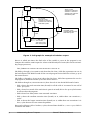
1
Bound-T time and stack analyzer
Reference Manual
Tid
rum
TR-RM-001
Issue 6.4
2013-11-28
Tidorum Ltd.
Tid
rum
Tidorum Ltd
www.tidorum.fi
Tiirasaarentie 32
FI-00200 Helsinki
Finland
This document, then a part of the Bound-T User Manual, was written at Space Systems Finland Ltd by
Niklas Holsti, Thomas Långbacka and Sami Saarinen.
The document is currently maintained at Tidorum Ltd by Niklas Holsti.
Copyright 2005 – 2013 Tidorum Ltd.
This document can be copied and distributed freely, in any format or medium, provided that it is kept
entire, with no deletions, insertions or changes, and that this copyright notice is included, prominently
displayed, and made applicable to all copies.
Document reference:
Document issue:
Document issue date:
Bound-T version:
Last change included:
Web location:
TR-RM-001
6.4
2013-11-28
3
BT-CH-0258
http://www.bound-t.com/manuals/ref-manual.pdf
Trademarks:
Bound-T is a trademark of Tidorum Ltd.
Credits:
This document was created with the free OpenOffice.org software, http://www.openoffice.org/.
2
Preface
The information in this document is believed to be complete and accurate when the document
is issued. However, Tidorum Ltd. reserves the right to make future changes in the technical
specifications of the product Bound-T described here. For the most recent version of this
document, please refer to http://www.bound-t.com/manuals/ref-manual.pdf.
If you have comments or questions on this document or the product, they are welcome via
electronic mail to the address [email protected] or via telephone, telefax, or ordinary mail to the
address given below.
Please note that our office is located in the time-zone GMT + 2 hours, and office hours are
9:00 - 16:00 local time. In summer daylight savings time makes the local time equal GMT + 3
hours.
Cordially,
Tidorum Ltd.
Telephone:
Fax:
Web:
E-mail:
+358 (0) 40 563 9186
+358 (0) 42 563 9186
http://www.tidorum.fi/
[email protected]
Mail:
Tiirasaarentie 32
FI-00200 Helsinki
Finland
Credits
The Bound-T tool was first developed by Space Systems Finland Ltd. (http://www.ssf.fi/) with
support from the European Space Agency (ESA/ESTEC). Free software has played an
important role; we are grateful to Ada Core Technology for the Gnat compiler, to William Pugh
and his group at the University of Maryland for the Omega system, to Michel Berkelaar for the
lp-solve program, to Mats Weber and EPFL-DI-LGL for Ada component libraries, and to Ted
Dennison for the OpenToken package. Call-graphs and flow-graphs from Bound-T are
displayed with the dot tool from AT&T Bell Laboratories. Some versions of Bound-T emit XML
data with the XML_EZ_Out package written by Marc Criley at McKae Technologies.
3
Contents
1
INTRODUCTION
1.1
1.2
1.3
1.4
2
3
5
4
62
Choice of outputs............................................................................................ 62
Basic output format........................................................................................ 62
List of unbounded program parts....................................................................69
Tabular output................................................................................................. 72
Detailed output............................................................................................... 77
DOT drawings..................................................................................................86
TROUBLESHOOTING
5.1
5.2
33
Basic form....................................................................................................... 33
Special forms.................................................................................................. 33
Naming root subprograms.............................................................................. 34
Options grouped by function...........................................................................36
Options in alphabetical order.......................................................................... 40
The help system..............................................................................................57
Patch files........................................................................................................ 58
Symbol definition files.....................................................................................60
UNDERSTANDING BOUND-T OUTPUTS
4.1
4.2
4.3
4.4
4.5
4.6
12
Introduction and overview.............................................................................. 12
How Bound-T analyses a program...................................................................12
Execution-time analysis.................................................................................. 21
Stack usage analysis.......................................................................................23
Context-specific analysis................................................................................ 26
Optional analysis parts................................................................................... 28
THE BOUND-T COMMAND LINE
3.1
3.2
3.3
3.4
3.5
3.6
3.7
3.8
4
What Bound-T is................................................................................................ 7
Overview of this Reference Manual...................................................................9
Other Bound-T documentation........................................................................ 10
Typographic conventions................................................................................ 11
ANALYSIS PROCESS
2.1
2.2
2.3
2.4
2.5
2.6
7
92
Warning messages.......................................................................................... 92
Error messages............................................................................................. 106
Tables
Table 1: Stable and unstable stacks.................................................................................................... 25
Table 2: Arithmetic model of bitwise Boolean operations................................................................. 28
Table 3: Options to select the analyses...............................................................................................36
Table 4: Options to name additional input files.................................................................................36
Table 5: Options to control the analysis............................................................................................. 37
Table 6: Options to choose outputs.................................................................................................... 38
Table 7: Options to control output format......................................................................................... 39
Table 8: Options for problem diagnosis.............................................................................................40
Table 9: Command-line options in alphabetical order...................................................................... 40
Table 10: Options for all drawings..................................................................................................... 49
Table 11: Options for call-graph drawings......................................................................................... 49
Table 12: Options for choosing subprograms for flow-graph drawings.............................................49
Table 13: Options for choosing the flow-graphs to be drawn............................................................ 50
Table 14: Options for flow-graph drawings........................................................................................50
Table 15: Options for the constant-propagation phase.......................................................................51
Table 16: Options for matching source-code file names..................................................................... 51
Table 17: File names for intermediate analysis files...........................................................................52
Table 18: Options for loop-bounds analysis....................................................................................... 52
Table 19: Options for detailed output.................................................................................................52
Table 20: Options for tracing............................................................................................................. 53
Table 21: Options for warnings.......................................................................................................... 56
Table 22: Options for virtual function calls........................................................................................ 57
Table 23: Help Option Forms............................................................................................................. 57
Table 24: Basic output fields.............................................................................................................. 62
Table 25: Basic output formats.......................................................................................................... 64
Table 26: Tabular output example..................................................................................................... 75
Table 27: Warning messages.............................................................................................................. 92
Table 28: Error messages................................................................................................................. 106
Figures
Figure 1: Inputs and outputs................................................................................................................ 9
Figure 2: Call-graph for example of tabular output........................................................................... 74
Figure 3: Call-graph of the tabular-output example.......................................................................... 76
Figure 4: Example non-recursive call graph...................................................................................... 88
Figure 5: Example graph of execution bounds.................................................................................. 88
Figure 6: Example recursive call graph.............................................................................................. 89
Figure 7: Example control-flow graph............................................................................................... 90
Figure 8: Example summary control-flow graph............................................................................... 91
5
Document change log
Issue
Section
Changes
6.4
Front matter
Added section for document change log.
All
Page numbers start from 1 for the cover page and continue sequentially from the
front matter to the body, for easier PDF handling.
Section 1.1
Added note on stack-usage analysis.
Section 2.2
Added discussion of tail calls and tail-call detection.
Section 2.3
Added a description of the modelling of volatile variables.
Section 3.4
Section 3.5
Updated and corrected tables of command-line options.
Section 3.6
Added this section to explain the new help system.
Section 4.2
Added description of Wcet_Loop output for the -loop_time option.
Section 5.1
Added misclassified tail calls as a possible reason for apparent recursion in the
target program, under the error message “Recursion detected”.
Section 5.2
Minor editorial corrections to error-message explanations.
6
1
INTRODUCTION
1.1
What Bound-T is
Bound-T is a tool for developing real-time software – computer programs that must run fast
enough, without fail.
The main function of Bound-T is to compute an upper bound on the worst-case execution
time (WCET) of a program or subprogram.
The function, “bound time”, inspired the name “Bound-T” pronounced as “bounty” or “boundtee”.
Bound-T can also compute an upper bound on the stack usage, thus making sure that the
program cannot fail due to stack overflow.
Real-time deadlines
A major difficulty in real-time programming is to verify that the program meets its run-time
timing constraints, for example the maximum time allowed for reacting to interrupts, or to
finish some computation.
Bound-T helps to answer questions such as
•
What is the maximum possible execution time of this interrupt handler? Is it less than the
required response time?
•
How long does it take to filter a block of input data? Will it be ready before the output
buffer is drained?
To answer such questions, you can use Bound-T to compute an upper bound on the execution
time of the subprogram concerned. If the subprogram cannot be interrupted by other
computations, and this upper bound is less or equal to the time allowed for the subprogram,
we know for sure that the subprogram will always finish in time.
When the program is concurrent (multi-threaded), with several threads or tasks interrupting
one another, the execution-time bounds for each thread can be combined to verify the timing
(schedulability) of the program as a whole. Such schedulability analysis is not a function of
Bound-T, but many schedulability analysis tools are available. Some tools are listed at
http://www.bound-t.com/scheduling-tools.html.
Static analysis - all cases covered
Timing constraints are traditionally addressed by measuring the execution time of a set of test
cases. However, it is often hard to be sure that the case with the largest possible execution time
is tested. In contrast, Bound-T analyses the program code statically and considers all possible
cases or paths of execution. Bound-T bounds are sure to contain the worst case.
Static analysis - no hardware required
Since Bound-T analyses rather than executes the target program, target-processor hardware is
not required. With the Bound-T approach, timing constraints can be verified without
complicated test harnesses, environment simulations or other tools that you would need for
really running the target program.
Of course, thorough software-development processes should include testing, but with Bound-T
the timing can be verified early, before the full test environment becomes available. In many
embedded-system development projects the hardware is not available until late in the project,
but Bound-T can be used as soon as some parts of the embedded target program are written.
Bound-T Reference Manual
Introduction
7
It’s impossible, but we do it with assertions
The task Bound-T tries to solve is generally impossible to automate fully. Finding out how
quickly the target program will finish is harder than finding out if it will ever finish – the
famously unsolvable “halting problem”. For brevity and clarity, this manual generally omits to
mention the possibility of unsolvable cases. So, when we say that Bound-T will do such and
such, it is always with the implied assumption that the problem is analysable and solvable with
the algorithms currently implemented in Bound-T.
For difficult target programs, the user can control and support Bound-T's automatic analysis
by giving assertions. An assertion is a statement about the target program that the user knows
to be true and that bounds some crucial aspect of the program's behaviour, for example the
maximum number of a times a certain loop is repeated.
Approximations
Also bear in mind that Bound-T produces an upper bound for the execution time, which may
be different from the exact worst-case time. Various approximations in Bound-T's analysis
algorithms may give over-estimated, too conservative bounds. However, the bounds can be
sharpened by suitable assertions.
Context and place
Figure 1 below illustrates the context in which Bound-T is used. The inputs are the compiled,
linked executable target program, an optional file of assertions, and command-line arguments
and options (not shown in the figure). The outputs are the bounds on execution time and stack
usage (optional), as well as control-flow graphs and call graphs (also optional).
Much depends on the target processor
Bound-T analyses the target program in its executable, machine-code form. This requires quite
a lot of target-specific knowledge, and so there is a different version of Bound-T for each type
of target processor. The proper version of Bound-T knows:
•
the format of the executable files for this target, and how to extract the code-memory
image, the constant data if any, and the symbolic debugging information from the file,
•
the binary encoding of the instructions for this target processor, and how to decode the
binary form into instructions,
•
the instruction set of this target processor, including which instructions control execution
flow (jumps, calls) and what each instruction computes,
•
the internal architecture of this target processor, and in particular how long it takes to
execute a given sequence of instructions (in the worst case, at least).
In some cases, Bound-T also has to know the calling protocols, register and stack usage conventions, and code-generation idioms of the cross-compiler(s) for the target processor.
A host computer is necessary, a target computer is not
The Bound-T tool itself is installed and executed on a host computer – your PC or workstation.
Since Bound-T works entirely by static analysis, not by measurement or profiling, it needs no
access to the target computer. You can use Bound-T to analyse a target program before the
target computer even exists, and before the target program is complete enough to be executed
on the target computer. All you need is a cross-compiler and linker that can generate the
machine code for the target processor.
8
Introduction
Bound-T Reference Manual
Source code
Libraries
Kernel
Compiler & linker
Find marks
Machine code
program
Source-code
mark positions
User assertions
on loop bounds,
variable values,
call counts, etc.
Bound-T
Enter Foo()
Main
Foo
Solve
Count
Ones
Static analysis:
- Decode instructions
- Trace control fl ow
- Trace subprogram calls
- Find loop bounds
- Find worst-case path
Main
. Foo
. . Count
. Solve
. . Count
. . Ones
9352
121
105
9207
303
721
Return
Flow graphs
Call graphs
Execution time bounds
Stack usage bounds
Figure 1: Inputs and outputs
1.2
Overview of this Reference Manual
What the reader should know
This Reference Manual explains the details of Bound-T's functions, its command-line options,
and its outputs. The reader is assumed to know in general how Bound-T works – for example
from reading the Bound-T User Guide – and how to program in some common procedural
(imperative) language, such as C or Ada. Familiarity with real-time and embedded systems is
an advantage. Most examples in the manual are presented in C, but Bound-T is independent of
the programming language, since it works on the executable machine code.
Bound-T Reference Manual
Introduction
9
Target program, target processor
To use Bound-T effectively, the user must also know the structure of the target program − the
program being analysed. In some cases, the user also needs to understand the architecture of
the target processor that will run the target program.
Reference Manual overview
This document is organised into chapters as follows:
1.3
•
Chapter 2 is an overview of the analysis process itself, divided into general analysis steps,
specific steps for execution-time analysis and for stack usage analysis, and optional steps.
•
Chapter 3 lists and explains all command-line options and arguments for Bound-T.
•
Chapter 4 explains all the outputs from Bound-T.
•
Chapter 5 lists warning messages and error messages, with explanations and advice on
solving the problems.
Other Bound-T documentation
This reference manual is supplemented by other documentation as follows.
User Guide
The Bound-T User Guide at http://www.bound-t.com/user-guide.pdf introduces Bound-T's
features and usage in an informal, tutorial way with examples. Read the User Guide to get
started, then return to this Reference Manual for details.
Assertion Language manuals
Most users of Bound-T need to write assertions to guide and constrain the analysis. Assertions
are written as text. The User Guide gives several examples of assertions. You can refer to the
Bound-T Asssertion Language manual at http://www.bound-t.com/assertion-lang.pdf for the
full syntax and meaning of the assertion language. The possible warning and error messages
from the assertion parser are also described there, not in this Reference Manual.
The find_marks program is an auxiliary program that lets you write assertions using marks
embedded in the source code to identify the loops or calls to which the assertion applies. Its
user manual is at http://www.bound-t.com/find-marks-manual.pdf .
Target-specific Application Notes
Bound-T is available for several target processors, with a specific version of Bound-T for each
processor. This Reference Manual describes only the general, target-independent features of
Bound-T. Additional information for specific targets is provided in separate Bound-T
Application Notes. When necessary, Application Notes also advise on using Bound-T with
specific target languages, compilers, real-time kernels or target operating systems.
Please refer to http://www.bound-t.com/app_notes for a list of the currently supported target
processors and the available Application Notes.
Hard Real Time programming model (HRT)
Bound-T contains special high-level support for target programs that follow the Hard-RealTime (HRT) programming model, an architectural style for concurrent, real-time programs
originally defined by the European Space Agency. This Reference Manual describes how
10
Introduction
Bound-T Reference Manual
Bound-T is used in its basic mode, without the special HRT features. There is a separate
manual that explains how to use Bound-T in HRT mode. See http://www.bound-t.com/hrtmanual.pdf.
1.4
Typographic conventions
We use the following fonts and styles to show the role of pieces of the text in this manual:
-option
symbol
text
keyword
A command-line option for Bound-T.
A mathematical symbol or variable.
Text quoted from a source file or a command.
A keyword (reserved word) in a programming language or in the Bound-T
assertion language.
Bound-T Reference Manual
Introduction
11
2
ANALYSIS PROCESS
2.1
Introduction and overview
This chapter gives a summary explanation of the analysis process. The summary shows what
Bound-T does, and in what order, but does not delve into the internal implementation. The
purpose of this explanation is to help you understand how you can control the analysis with
command-line options (to be defined in the next chapter) and with assertions (as shown in the
User Guide and defined in the Assertion Language manual).
The order of explanation follows the (normal) order of the analysis steps:
•
loading the executable code and the symbolic debugging information,
•
decoding instructions and building control-flow graphs and the call-graph,
•
analysing the computations to find bounds on variable values, loop repetitions, and other
dynamic behaviour,
•
computing WCET bounds, if desired, and
•
computing stack-usage bounds, if desired.
The final section of the chapter explains some of the optional, but normally included, analysis
steps: arithmetic interpretation of bit-wise Boolean operations; constant propagation; valueorigin analysis; and pruning flow-graphs to remove infeasible parts.
The text in this chapter assumes that Bound-T is used in the “basic” mode, not in the HRT
mode. All the analysis steps in the basic mode are also used in the HRT mode, but the HRT
mode first reads the HRT model file (the TPOF), then performs the analysis, and finally
generates the HRT execution-skeleton file (the ESF) that combines the TPOF with the
computed WCET bounds. For more information please refer to the HRT-mode manual at
http://www.bound-t.com/hrt-manual.pdf.
2.2
How Bound-T analyses a program
This section explains the initial steps in the analysis, common to execution-time analysis and
stack-usage analysis: loading the executable code, creating control-flow graphs and the callgraph, and analysing the computations.
Loading the executable program
The first thing that Bound-T does (after scanning the command-line parameters, of course) is
to open and read the file that contains the executable code of the target program to be
analysed. The details of this process depend on the format of the file – ELF, COFF, or
something else – but the result is always the same:
•
a memory image that represents the contents of the target-computer memory after the
target program code (and constant data) are loaded, immediately before the target program
starts execution,
•
a symbol table that connects source-code identifiers (subprogram names, variable names,
type names and definitions) to machine-level entities (code addresses, registers, datamemory addresses and offsets),
•
a source-line table that connects locations in source-code files (file name, line number,
perhaps column number) to machine-code locations (code address).
The memory image is usually only a partial image; it defines the initial contents of some
memory locations (usually code) but not of all locations (usually data).
12
Analysis process
Bound-T Reference Manual
The symbol table and source-line table may be more or less complete, depending on the
compilation and linking options used when the executable file was generated (for example, -g
for gcc) and on the general ability of the compiler, linker, and the executable-file format to
transmit and represent such information. For example, an executable program given as an
“Intel Hex” file has no symbol table or source-line information, while a UBROF file from an
IAR Systems compiler has very extensive information (much more than Bound-T can use at
present).
Bound-T's analysis is based almost entirely on the memory image. Bound-T uses the symbol
table and the source-line table only to translate user-provided source-level input (for example,
the names of root subprograms) into machine-level terms for the analysis, and vice versa on
output of analysis results.
The program model
Static program analysis needs a program to analyse. For imperative (procedural) programs
this means a representation of the atomic actions (statements, instructions) that the program
can execute, and a representation of the order in which the actions may be executed (execution
paths, flow of control). It is common to divide the program into subprograms and to divide the
execution flow into jumps within a subprogram on the one hand, and calls between
subprograms on the other. Bound-T follows this approach.
Bound-T analyses machine-code programs and so:
•
the atomic actions are machine instructions,
•
the subprograms are sets of machine instructions,
•
execution flow within a subprogram is represented by a control-flow graph that contains all
the machine instructions of the subprogram, groups them into basic blocks (graph nodes)
and shows how execution can flow from node to node (graph edges),
•
execution flow between subprograms is represented by a call-graph that has a node for
every subprogram and an edge for every call from one subprogram to another.
It is important to understand that this structure (subprograms, control-flow graphs, call
graphs) is not explicit in the executable file. The memory image is usually a homogeneous octet
sequence, with no evident boundaries between the octets that form machine instructions and
the octets that represent other things, for example constant data tables, tables of addresses for
switch-case statements, or just padding for alignment purposes.
The only reliable connection between source-code subprograms and the memory image is
found in the symbol-table that gives the entry address of each subprogram.
Bound-T therefore builds its program model by an iterative, interpretive, bottom-up process
that starts with these entry addresses, the memory image, and nothing else (well, some
command-line options and assertions can help).
Decoding instructions and tracing the flow of control
Bound-T builds its program model subprogram by subprogram, starting from the root
subprograms named on the command line.
To build the control-flow graph of a subprogram, we start with the entry address of the
subprogram and:
•
fetch and decode the instruction at the entry address, from the memory image,
•
insert the instruction in the flow-graph of this subprogram, if not already there,
•
if the instruction is return-from-subprogram, we are done with this instruction, else
•
find the successors of the instruction, that is, the addresses of the instruction(s) that are
executed next, in this same subprogram,
Bound-T Reference Manual
Analysis process
13
•
fetch and decode the successor instructions in the same way, if they are not already in the
flow-graph, until all instructions for this subprogram have been found, decoded, and
inserted in the control-flow graph.
When a call instruction is found the address of the callee is memorized and taken as the entry
address of a new subprogram which is then processed in the same way. Each subprogram is
entered as a node in the call-graph and each call instruction is entered as an edge in the callgraph. Thus, the final program model contains all and only the subprograms that can be called
from the root subprograms, directly or through other subprograms.
If all jump instructions and call instructions have static targets (as opposed to dynamic,
register-indirect jumps and calls) the above algorithm evidently works.
You can observe this algorithm on the fly with the Bound-T options -trace decode or -trace
effect. Either option makes Bound-T output, for each instruction that it fetches and decodes,
the address of the instruction, the machine-code instruction itself (usually in hexadecimal),
and the disassembled form of the instruction. The option -trace effect gives some more
information that is not interesting at this point. We will return to it.
Calls and call steps
When the flow-graph-building algorithm finds a call to another subprogram, it inserts the call
instruction in the caller's flow-graph in the normal way. Furthermore, at the point in the flowgraph where execution flows into the callee, the algorithm inserts a special flow-graph
element, a call step, that is similar to an instruction but is a place-holder that represents the
execution of all the instructions in the callee, up to and including the return to the caller.
In the caller's flow-graph (under construction now) the successors of the call-step are the
return points in the caller. Usually there is exactly one return point, and usually this is the
instruction immediately after the call instruction, but in some cases the return point may be
somewhere else, or there may be several possible return points, or none at all for a nonreturning callee.
In the usual case, after inserting the call-step (and possibly memorizing the callee as a new
subprogram) the flow-graph-building algorithm goes on to the successors of the call-step.
Thus, the algorithm aims to complete the flow-graph of the caller, before building the flowgraph of the callee.
Tail calls
When the last action in a subprogram is to call another subprogram, it is sometimes possible to
implement the call by a simple jump instruction to the entry point of the callee, without saving
a return address to the caller. This is known as an (optimized) tail call. When the callee
eventually returns, control does not transfer back to the caller but to some higher-level
subprogram, usually the caller of the caller. If Bound-T models and analyses such a jump
instruction in the normal way, as a transfer of control within the same flow-graph, the callee's
instructions become part of the caller's flow-graph and the call is not recorded in the call
graph. To avoid this, Bound-T tries to detect when a jump instruction implements a tail call.
The details are target-specific but in general Bound-T classifies a jump instruction as a tail call
if both the following conditions hold:
•
The target address is known to Bound-T as the entry point of a subprogram, either from the
program's symbol table (debugging information) or from an assertion that uses this
address, or a symbol connected to this address, to identify a subprogram.
•
The target address is not the entry point of the current subprogram (the subprogram that
contains the jump instruction). (If a jump instruction back to the entry point of the current
subprogram were modelled as a tail call, it would represent direct (tail) recursion, and
Bound-T cannot model recursion.)
The command-line option -no_tail_calls disables this tail-call detection. Bound-T then models
only explicit call instructions as calls. There may be further target-specific options to control
tail-call detection in detail; check the relevant Application Notes.
14
Analysis process
Bound-T Reference Manual
Handling dynamic flow of control
While building the control-flow graph of a subprogram, Bound-T may find a jump instruction
or a call instruction in which the target address is not statically defined but is computed
dynamically, typically taken from a register (a register-indirect jump or call). When this
happens Bound-T inserts the instruction in the flow-graph in the normal way. Since the
successor instructions are not yet known, Bound-T then suspends the building of (that part of
the) flow-graph and instead inserts a special object in the flow-graph to represent the dynamic
jump or the dynamic call, in the hope that the later analysis of the computations may resolve
the target address or addresses into some known values.
This means that the flow-graph building algorithm given above may produce either a complete
flow-graph, with all jumps and calls statically resolved, or an incomplete flow-graph that
contains some unresolved dynamic jumps or calls – truncated paths, as it were, at which the
execution flows into unknown parts of the subprogram or program.
If the later analysis of the computations in the incomplete flow-graph resolves some or all of
the dynamic jumps and reveals the actual successor instructions, the suspended flow-graph
building algorithm is resumed to extend the flow-graph with these instructions, their
successors, and so on. More than one such cycle of suspension-analysis-resumption may be
necessary to complete the flow-graph.
Dynamic calls can be resolved by analysis but can also be resolved by assertions. An assertion
can list all the possible callees of a given dynamic call; Bound-T will then insert the corresponding call-steps in the flow-graph, as successors of the dynamic call instruction and
predecessors of the return points. This corresponds to a non-deterministic choice between the
possible callees at this point in the flow-graph. A similar flow-graph structure results when a
dynamic call is resolved by analysis and several possible callees are found.
Finally, the return point of a call may also be defined by a dynamic computation; this is
handled as if the call step contained a dynamic jump and had no statically known successors.
The static or dynamic definition of the callee is independent of the static or dynamic definition
of the return point; all four combinations are possible. However, if the call and return are both
dynamic, the call is resolved before the return, and the resolution of the return can be different
for each possible callee.
Properties of instructions and control-flow edges in the program model
When Bound-T decodes instructions and enters them in the flow-graph of a subprogram it
provides each instruction with two main properties:
•
the arithmetic effect of the instruction, which is represented as a set of assignments of the
form c := e, where c is a storage cell (a register or a memory reference) and e is an
arithmetic expression formed of constants and storage cells; and
•
the computational effort of the instruction, which is a target-specific representation of the
actions that the target processor takes to execute the instruction, with focus on the time
(number of cycles) required.
For a simple target processor, an “effort” may be just a number of cycles. For a more complex
processor, with parallel or pipelined computational units, an “effort” may be a structure with
several components that detail the actions that the instruction requires of each computational
unit.
The difference between the options -trace decode and -trace effect is that the latter also displays
the arithmetic effect of each decoded instruction (which can create rather long output lines).
At this point in the analysis, call steps in a flow-graph have a null effect and a null effort. Later
on, each call-step will be provided with an effect that is a summary of the effect of the callee
subprogram, and an effort (expressed directly in execution time) that is an upper bound on the
execution time of the callee.
Bound-T Reference Manual
Analysis process
15
The edges (arcs) in a flow-graph represent execution flow from instruction to instruction.
Bound-T provides each edge with two attributes (in addition to the identities of the source and
target instructions):
•
the condition of the edge, represented by a Boolean expression of storage cells; and
•
the execution time of the edge, represented as a number of cycles, often zero.
The condition of an edge is a necessary but perhaps not sufficient condition for “taking” the
edge during execution. That is, execution can flow along the edge only if the condition is true,
but a true condition does not force the edge to be taken. However, for conditional jump
instructions the conditions on the two possible edges are often logically complementary, and
then both of them are both necessary and sufficient.
The analysis of execution time (WCET) is based on
•
the effort assigned to each instruction,
•
the execution time assigned to each edge, and
•
the loop repetition bounds and other control-flow constraints derived from the instruction
effects and edge conditions.
The analysis of stack usage is based on
•
the instruction effects, when they modify the storage cells that are stack pointers,
•
the edge conditions, when they depend on stack pointer values.
Multiple representations of the same instruction
The informal presentation of the flow-graph-building algorithm, above, may have given the
impression that a certain instruction (at a certain address in the memory image) can appear
only once in a flow-graph. This is not so; there are several reasons why a given instruction can
occur multiple times in the same flow-graph (same subprogram) or in different flow-graphs for
different subprograms, as follows:
•
The instruction is reached from several entry addresses.
Bound-T considers each distinct entry address to define a distinct subprogram, even if the
execution then flows into “shared” instructions that are reached from several entry addresses.
Bound-T builds a separate flow-graph starting from each entry address, thus the shared
instructions will appear in every flow-graph that reaches them. Compiler optimizations that
change “tail calls” into jump instructions often lead to such shared instructions.
•
The instruction is in a special subprogram (typically a compiler-supplied prelude or postlude routine) that is defined to be “integrated” into the flow-graphs of callers.
When a subprogram is defined to be “integrated” (by a user assertion, or automatically by
Bound-T) any call to this subprogram is processed as if it were a jump, with the result that the
instructions of the “integrated” subprogram are inserted in the flow-graph of the caller. In
effect, this “inlines” the callee into the caller for the analysis. Each instruction of the
“integrated” subprogram is thus represented in the flow-graph of each caller, perhaps multiple
times if the same caller has multiple calls to the same “integrated” subprogram.
•
The instruction lies within a (target-specific) idiomatic instruction sequence that has a
specific combined effect and is therefore represented as one atomic part of the flow-graph.
An example of such an idiomatic instruction sequence is an 8-bit-wide addition instruction
immediately followed by an 8-bit-wide addition-with-carry, such that the instruction pair
implements a 16-bit-wide addition operation. For some target processors Bound-T pairs such
instructions in the flow-graph to give a 16-bit-wide arithmetic effect. However, if a jump
instruction leads to the second instruction (add with carry) but bypasses the first instruction
(add), this second instruction is represented a second time in the flow-graph, with only its 8bit-wide effect.
•
16
The instruction is a delay instruction of a delayed conditional jump.
Analysis process
Bound-T Reference Manual
Pipelined processors sometimes have delayed jumps (and calls, but that is not relevant here)
in which the processor executes one or a few “delay instructions” consecutively after the jump
instruction, because these instructions are already in the pipeline, before control transfers to
the jump target. For a conditional jump the delay instructions are executed whether or not the
jump is “taken”. For such processors Bound-T makes the flow-graph branch immediately after
the conditional jump instruction, and therefore Bound-T represents each delay instruction
twice, once in the “jump taken” branch of the flow-graph, and once more in the “jump not
taken” branch. Some cases of consecutive jump instructions may generate more than two
representations of the delay instructions in their different roles.
•
The instruction is subject to partial evaluation.
During the flow-graph-building algorithm Bound-T normally tracks only a small part of the
state of the target processor, to wit, the program counter (PC), or the small set of program
counters that identifies the instructions in the pipeline, when there is a pipeline. However, for
some purposes it is useful to track and evaluate a larger part of the state, for example the
values held in the target-processor registers. The algorithm is then extended to evaluate the
arithmetic effect of each instruction on the fly. This evaluation is only partial because the effect
may use unknown parts of the target-processor state, and then the result of the evaluation may
also be unknown. Anyway, when this partial evaluation is going on Bound-T tags each
instruction, when inserted in the flow-graph, with the state in which the instruction was
evaluated. If the code under evaluation contains loops – as it usually does – the same
instruction will be evaluated in multiple states and will thus occur multiple times in the flowgraph.
At present, partial evaluation is used only for some forms of code generated for switch-case
statements1. Some compilers implement (some) switch-case statements by generating a
constant table of values and jump addresses, and calling a library routine to interpret the table
at run-time. To analyse such a switch-case statement Bound-T partially evaluates the
interpretive routine with respect to the constant table. The result is an expanded copy of the
interpretive routine, integrated within the flow-graph of the subprogram that contains the
switch-case statement.
Finding the loops
When a flow-graph is ready for further analysis (whether complete, or incomplete with
dynamic jumps or calls) the next step is to discover its loop structure. Bound-T uses the simple
definition of “natural loop” which means that a loop structure can be found only when the
flow-graph has a reducible structure. The natural loops in a reducible flow-graph form a clean
hierarchy – two loops are either completely separate, or one is nested within the other – and
each loop has a single entry point, the loop head node.
When a flow-graph is irreducible Bound-T cannot divide it into such a loop hierarchy. An
irreducible flow-graph always has some cycles, thus the execution paths are potentially
unbounded, but Bound-T cannot use its loop-bound analysis nor can it accept assertions on
loop bounds – because there are no loops that Bound-T knows about.
Irreducibility does not hamper stack-usage analysis, but execution-time analysis will be
possible only when assertions on the number of repetitions of other parts of the flow-graph (in
particular, calls) are enough to bound all execution paths. For more information on this point
please refer to the Assertion Language manual and the “enough for time” assertion.
You can observe the loop structure (for reducible flow-graphs) with the Bound-T option -trace
loops, but it is probably easier to view the loops in the DOT drawings of the flow-graphs, using
the options -dot and -draw with suitable arguments. The loop heads are marked as such in the
drawings. “Forward” execution edges usually point downwards in the drawings, so the “back”
edges that represent loop repetition are easy to spot, because they usually point upwards to a
loop head.
1 See N. Holsti, “Analysing Switch-Case Tables by Partial Evaluation”,
7th International Workshop on Worst-Case Execution Time Analysis (WCET'2007), Pisa, Italy, July 3,
2007.
http://www.bound-t.com/reports/wcet2007/abstract.html.
Bound-T Reference Manual
Analysis process
17
Analysing the computations
WCET analysis would be far simpler if programs had no conditional jump instructions. Since
most processors have them, the input data, and whatever data is computed from the inputs,
can influence the flow of control – the execution paths – and thus determine the execution
time.
It is therefore useful – even necessary – to study the computations of the program under
analysis. The general goal is to understand how the computation influences the execution flow,
and in particular to
•
resolve the actual targets of computed (dynamic) jumps and calls,
•
resolve or bound the actual addresses used in computed (indirect) memory references,
•
put bounds on the number of loop repetitions, by correlating the termination or repetition
condition with the computations in the loop body.
In fact the second point – resolving computed memory references – is more a means than a
goal. Such references have no direct effect on execution flow, but have an indirect effect by
changing or using particular data on which some conditional or computed jump depends.
For Bound-T, the computation that a subprogram executes is represented in the flow-graph by
the arithmetic effects of the instructions and the conditions of the edges. Bound-T applies
several kinds of analysis on this representation:
•
Constant propagation evaluates expressions that have constant (static, literal, immediate)
operands and propagates the results, when constant, into storage cells and other
expressions that use those storage cells. The result is a simplified set of arithmetic effects
and edge conditions – a refined computation model for the flow-graph and subprogram.
•
Value-origin analysis matches each use of a storage cell (in the effect of an instruction or in
the condition of an edge) to the instructions that might define the value that is used (by an
assignment to this storage cell in the instruction's effect). The result is similar to a Static
Single Assignment representation of the data-flow. Bound-T uses the result to detect
storage cells that are invariant over the execution of a subprogram, and for some special
things such as detecting when a dynamic jump is in fact a return from the subprogram
because the computed target address is the return address.
•
Presburger analysis (also called arithmetic analysis in Bound-T) models the effect of each
instruction as a relation between the (integer) values of storage cells before the instruction,
and their values after the instruction. This transfer relation is expressed in Presburger
Arithmetic. The transfer relation for an instruction sequence is formed by joining
(chaining) the transfer relations for each instruction. When passing over an edge, the
transfer relation is intersected (conjoined) with the edge condition. Where several edges
converge on the same node, the transfer relations from each edge are united (disjoined).
The result is the transfer relation for the whole flow-graph or for a selected part, for
example for the body of a loop.
The whole analysis can be repeated in a context-specific way for a particular call-path leading
to the subprogram. The call-path provides values or bounds on some of the parameters of the
subprogram. For example, constant propagation and Presburger analysis can “specialise” the
computations in the subprogram for the parameter values given in a particular call, and that,
in turn, can lead to call-specific loop bounds and a call-specific WCET bound.
Resolving dynamic jumps
When a flow-graph contains a dynamic jump, that is a jump where the target address is
computed in some way, Bound-T tries to resolve the jump targets by using the several forms of
analysis of the computation.
Programs can use dynamic jumps for various purposes; the analysis in Bound-T is aimed in
particular at dynamic jumps that implement switch-case control structures. Such dynamic
jumps often have several possible targets (the different case branches in the switch-case
18
Analysis process
Bound-T Reference Manual
structure). Constant propagation can supply only one target value; therefore, dynamic jumps
for switch-case structures are usually resolved by the Presburger analysis, which can supply
several target values.
However, even for the powerful Presburger analysis, Bound-T must often first recognize the
dynamic jump as a part of a target-specific instruction sequence, or pattern, that implements a
particular form of switch-case code. For example, some densely indexed switch-case structures
are implemented by a constant table of case-addresses which is indexed by the switch index.
The instruction pattern consists of instructions that load an address from this table and jump
to this address. When Bound-T recognizes this sequence it can use the Presburger analysis to
bound the index, thus to find the start and end of the table, and thus to find the possible target
addresses (by fetching them from the table in the memory image).
The most complex form of switch-case code needs the partial evaluation analysis, as explained
earlier. However, for such code the dynamic jumps are often resolved by the partial evaluation
itself, without further analysis of the residual flow-graph.
After resolving dynamic jumps Bound-T resumes the flow-graph-building algorithm to
complete the flow-graph, as explained earlier.
Your can use the Bound-T option -trace resolve to observe the details of the resolution of
dynamic jumps and calls.
Resolving dynamic calls and returns
Bound-T tries to resolve dynamic calls and returns in the same way as it resolves dynamic
jumps. However, dynamic calls can also be resolved by assertions, which is not possible for
dynamic jumps.
If the call is dynamic, but the return point is static, each resolved callee adds only a new call
step to the flow-graph (and an entry in the call-graph), but it is not necessary to resume the
flow-graph-building algorithm – no new instructions in the caller subprogram are reached. If
the return point is dynamic it may be resolved into new instructions, not yet in the flow-graph,
and then flow-graph building must resume.
Resolving dynamic memory references
Most programs make many memory references with dynamic, computed addresses. For
example, most accesses via pointers, or via index variables to arrays, result in such dynamic
memory references. But most of these memory references are unimportant for the flow of
execution, such as loop termination. Bound-T can use its analysis of the computation to try to
resolve dynamic memory references:
•
Constant propagation is applied to all dynamic memory references, both reads and writes
and in all parts of instruction effects and edge conditions.
•
Presburger analysis is applied by default only to references that are used (read memory) in
expressions that assign values to storage cells that are relevant for the analysis of execution
flow. The option -arith_ref can be used to extend this analysis to all dynamic memory
references or to turn it off completely.
Most useful resolution of dynamic memory references happens by constant propagation,
because Bound-T can at present make use only of references that are resolved to a single actual
memory address. Most such references are to data in a stack, and are dynamic only because
the stack pointer (to be precise, the local stack height) is dynamic. The offset in the stack frame
is usually static.
The Presburger analysis, especially when applied to indexed array references, usually gives
intervals (ranges) of memory addresses, which are useless to Bound-T at present.
When a dynamic memory reference is resolved to a single memory address, this address
defines a storage cell that takes part in the computation. If this storage cell was not explicitly
(statically) referenced before, in the initial instruction effects created by instruction decoding,
Bound-T Reference Manual
Analysis process
19
the computation model is extended to include this cell and the analysis of the computation is
repeated. Thus, constant propagation etc. may be applied two or more times to the same flowgraph, iteratively extending the set of storage cells that take part in the computation.
Modelling volatile storage cells
Most processors have "memory" addresses which are mapped to active devices, for example
I/O ports, rather than passive memory devices, with the result that the data read from such an
address is not necessarily equal to the data last written to the same address. For example, an
address mapped to a parallel-input port usually returns the current logical levels of the input
signals, which can vary rapidly and unpredictably from one reading of this address to the next.
In programming languages such as Ada or C, such non-memory addressable locations are
called volatile. It is usually necessary to mark such variables explicitly in the source code, in C
with the keyword volatile; in Ada with the pragma Volatile. This tells the compiler that it must
preserve the existence and order of all reads and writes to those variables and must not assume
that a read following a write returns the written value, nor that successive reads return the
same value.
Another kind of volatile variable is a "shared" variable that is used and altered by more than
one thread or task. If the execution of those tasks can be interleaved, and especially if a task
switch can occur at unpredictable times due to interrupts or pre-emptions, then a shared
variable can indeed appear volatile from the point of view of one task, because other tasks can
assign new values to the variable at any time.
The data-flow analysis in Bound-T must know about such volatility of "storage" locations, that
is, what Bound-T considers storage cells. Otherwise, the analysis may make false conclusions
leading to underestimated time and stack requirements. For example, assume that the storage
cell c is such a volatile location and that the program under analysis contains two successive
instructions which load c into registers r1 and r2, respectively, followed by conditional branch
if r1 is not equal to r2. If Bound-T is not aware that c is volatile, both the value-origin analysis
and the arithmetic analysis will conclude that r1 must be equal to r2, since they are both copies
of the same value of c, and therefore the condition is always false and the branch is never
taken. This false conclusion could wrongly exclude major parts of the code from the analysis of
execution time and stack usage.
To avoid such problems, Bound-T allows storage cells to be marked as volatile, either in
assertions or by default markings which are target-specific. (Currently only global cells can be
volatile, not cells local to a subprogram.) For example, a given processor architecture may
reserve a certain address range for memory-mapped I/O devices, and Bound-T for that
processor could then assume that all storage cells in that range are volatile. Such default
volatility assumptions are documented in the Application Notes for the processors concerned.
Here we explain how Bound-T models volatile storage cells in its several analyses.
Perhaps it seems evident that volatile cells should be modelled by always considering any value
read from a volatile cell as unknown (opaque). However, we want to let users assert bounds on
the values of volatile cells, and to use those bounds in the analysis, which is easier to do if a
somewhat different model is used, as follows.
Constant-propagation analysis ignores all assignments (writes) to a volatile cell, while
analysing uses (reads) of a volatile cell in the same way as for non-volatile cells. In the absence
of assertions on the value of the volatile cell, this means that the cell's value is modelled as
unknown (opaque). However, if the user asserts a single value for the volatile cell, this value
becomes available to the analysis as a constant and can be propagated into computations and
conditions.
Value-origin analysis is applied only to non-volatile cells and does not try to find the origins of
the values of volatile cells. If a non-volatile cell is assigned the value of a volatile cell, this
assignment becomes the origin of the value of the assigned cell, and this value has no other
origin.
Live-variable analysis considers only non-volatile cells to be "live". However, an expression
that uses both volatile and non-volatile variables can be "live", and then makes those nonvolatile cells "live", too. This, again, supports assertions on the values of volatile cells. For
20
Analysis process
Bound-T Reference Manual
example, if v is a volatile cell with no value assertions, and x is a non-volatile cell, the "live"
expression v+x can take any value, whatever value x has. However, if we know (from an
assertion) that v is between 2 and 5, then bounds on x lead to bounds on v+x and therefore x is
"live" at this point in the program.
Arithmetic analysis includes volatile cells, but the Presburger relation which models a flowgraph step defines no relation between the value of a volatile cell, after the step, and the value
of any other cell or expression, before or after the step. In effect, any use of a volatile cell
returns an unknown (opaque) value, only limited by the assertions, if any, on the value of the
cell. However, if the same volatile cell is used several times in one and the same step, this
model assumes that the same value results from each use. This feature of the arithmetic model
must be taken into account in the processor-specific instruction decoders and flow-graph
builders in each version of Bound-T. For example, if the processor has an instruction sub r,x,y
which subtracts two memory operands x and y and stores the result into a register r, and the
program applies this instruction to a volatile memory location v in the form sub r,v,v, and if
the two reads of v in this single instruction can return different values, then the flow-graph
builder must divide this instruction into two flow-graph steps where each step reads v once. If,
instead, the instruction is modelled as one step with the effect r := v ‒ v, then the arithmetic
analysis would see this effect as r := 0, which would be incorrect.
2.3
Execution-time analysis
Execution-time (WCET) analysis is an optional step in Bound-T, enabled with the option -time
and disabled with -no_time. The option is enabled by default.
Execution-time analysis follows (or calls for) the various analyses of the computation, and
consists of three parts:
•
bounding loop repetitions,
•
finding execution-time bounds on flow-graph nodes (basic blocks), and
•
calculating the WCET bound with the IPET method.
Bounding loop repetitions
The loop-bound analysis in Bound-T is aimed at counter-controlled loops, where the loop
termination is controlled by one (or several) loop counters. A loop counter is a program
variable (represented as a storage cell in Bound-T) that is initialized to an initial value before
the loop, increased (or decreased) by a non-zero value on each repetition of the loop, and is
used in the loop termination or repetition condition in such a way that the loop can be
repeated only while the variable is less than (or greater than) a limit value. The initial value,
increment or decrement, and limit value must all be known constants, or have known ranges,
at this point in the analysis (that is, after the constant propagation, possibly including
propagation of context-dependent parameter values).
Accordingly, Bound-T analyses each loop as follows:
•
find possible counter variables by studying the Presburger transfer relation for the loop
body (from and including the loop head up to an edge that repeats the loop) to detect which
storage cells have a bounded and non-zero increment or decrement (of constant sign); such
storage cells are candidates for loop counters,
•
for each such loop-counter candidate, use the Presburger relation for the values of storage
cells on entry (initialization) of the loop to compute bounds on the initial value, and retain
only those candidates where the initial value is bounded in a direction that matches the sign
of the increment or decrement,
•
for each remaining loop-counter candidate, use the Presburer relation for the values of
storage cells on the loop's repeat edges (“back” edges) to see if there is a complementary
limit on the values of the counter that permit repetition of the loop.
Bound-T Reference Manual
Execution-time analysis
21
If one or more such controlling loop-counter cells are found, a simple computation involving
the initial value (bounds), the increment or decrement (bounds), and the limit value for
repetition gives an upper bound on the number of repetitions of the loop. A lower bound could
often also be computed, but Bound-T does not compute one because it does not do “best case”
analysis.
If more than one controlling loop-counter cell is found, Bound-T of course takes the smallest
computed loop-repetition bound.
Bound-T reports the computed loop-bounds using output lines that start with the keyword
Loop_Bound.
Assigning execution times to flow-graph nodes and edges
As explained above, each instruction in the flow-graph is provided with a “computational
effort” quantity. Instructions are collected into basic blocks, which are the nodes in the flowgraph; each node thus corresponds to a sequence of instructions. For computing bounds on
the execution time, we need a bound on the execution time of each node. Since the concept of
“effort” is target-specific, there is a target-specific procedure for combining the efforts of the
instructions in a node (a basic block) to give an upper bound on the execution time of the
whole instruction sequence in the node.
For a simple, purely sequential target processor, where the “effort” is simply the number of
cycles required by the instruction, this combination procedure just adds the numbers to give a
total number of cycles for the node. For more complex processors the combination procedure
may be correspondingly more complex, for example it may consider overlapping execution of
the instructions.
Calls from one subprogram to another are a special case. As explained earlier, each call from a
subprogram to another is represented by a call-step in the caller's flow-graph. When
instructions are collected into nodes, each call-step becomes a node of its own – a call node.
Later in the analysis, the execution time of this node is set to the upper bound on the execution
time of the callee (possibly context-specific).
As also explained above, each edge (flow transition) between instructions in the flow-graph is
provided with an (upper bound on the) execution time, as a number of cycles. When the
instructions are collected into basic-block nodes, some of these edges become internal to a
node and some become edges between nodes. The execution times of edges that are internal to
a node are included in the target-specific combination procedure that computes the upper
bound on the execution time of the node. The execution times of edges between nodes are used
directly in the IPET procedure, described below.
Using IPET with lp_solve
At this point in the analysis the call-graph has been expanded into a graph of “execution
bounds”, where the main difference is that a given subprogram or a given call (site) may have
several different execution bounds, specific to certain call paths, as will be explained in
section 2.5. Each such execution-bounds object gives:
•
bounds on the repetition of the loops in the subprogram,
•
possibly other derived or asserted bounds on the execution paths within the subprogram,
for example infeasible parts of the flow-graph,
•
an upper bound on the execution time of each flow-graph node (basic block), except for
call-nodes, and
•
an upper bound on the execution time of each flow-graph edge between nodes.
Bound-T now uses the Implicit Path Enumeration Technique (IPET) to compute an upper
bound on the execution time, or WCET. In this method, the problem is translated into an
Integer Linear Programming (ILP) form, where
•
22
the unknown integer variables represent the number of executions of each flow-graph node
and edge,
Execution-time analysis
Bound-T Reference Manual
•
the objective function to be maximized is the total execution time (bound), which is simply
the sum of the (known bound on the) execution time of each node and edge multiplied by
its (unknown) number of executions, and
•
the unknown execution-count variables are constrained by the loop-repetition bounds and
by the “structural” constraints, similar to the Kirchhoff rules: the number of executions of a
node equals the total number of executions of edges that enter the node, and also equals the
total number of executions of edges that leave the node, with special cases for the entry
node and return nodes.
An ILP solver then produces a solution (the number of executions of each node and edge) that
gives a maximal value of the objective function, an upper bound on the WCET. Bound-T uses
the lp_solve program to solve the ILP problem.
The IPET method is applied bottom-up in the graph of execution bounds, starting from the
lowest level (leaf subprograms) and proceeding to higher levels (towards the root
subprograms). Thus, when we apply IPET to a given subprogram we know the bounds on the
execution time of all lower-level subprograms, which gives the bounds on the execution time of
all call nodes at this level.
Bound-T reports the computed WCET bounds using output lines that start with the keyword
Wcet (for context-independent bounds) or Wcet_Call (for context-specific bounds).
You can observe the IPET procedure with the Bound-T option -keep_files (on Linux platforms).
Bound-T interacts with lp_solve through text pipes; this option stores the lp_solve input and
output as text files. The option -show counts shows just the IPET solution, the execution counts
of each node and edge. The execution counts are also shown in the flow-graph drawings ( -dot
and -draw options).
HRT mode
The HRT mode of Bound-T implements all of the above analysis steps in the same way.
However, after computing the execution-time bounds, the HRT mode generates the Execution
Skeleton File (ESF) that defines the real-time architecture of the target program (its tasks and
its protected objects) and moreover gives the WCET bounds.
2.4
Stack usage analysis
Stack-usage analysis is an optional step in Bound-T, enabled with the options -stack or
-stack_path and disabled with -no_stack. Stack usage analysis is disabled by default.
Stack-usage analysis follows (or calls for) the various analyses of the computation, and consists
of two parts:
•
finding upper bounds on the local stack height in each subprogram, and in particular at
each call within the subprogram, and
•
collecting those local upper bounds, along call-paths in the call graph, to find an upper
bound on the total stack usage (local + callees) for each subprogram, up to and including
the root subprograms.
Stack mechanisms
Different target processors have very different stack mechanisms. The most common
mechanism are these, from simple to complex:
•
no hardware stack at all,
•
a fixed-size stack that is used only for return addresses and cannot be used for data,
•
a stack in main memory that is used both for return addresses and for data and has a
software-defined size.
Bound-T Reference Manual
Stack usage analysis
23
The processor may have special instructions for accessing the stack, for example “push” and
“pop” instructions. The processor may have general-purpose instructions that are also suitable
for stack operations, for example load and store instructions with register-indirect addressing
and auto-increment or auto-decrement of the pointer register.
For small hardware stacks that only hold return addresses, the software usually has no choice
in how it uses the stack. When the processor hardware is not so constraining, the processor
manufacturer sometimes defines software rules for passing parameters and using the stack for
local variables.
Multiple stacks and stack names
When the processor's hardware stack holds only return addresses, but the programming
language provides subprograms that may be reentrant or recursive, it is common for the
compiler (or indeed an assembly-language programmer) to define a second software stack for
parameters and local variables. Thus, some target programs use two stacks, hardware and
software, or perhaps even several software stacks for different purposes. Software stacks are of
course used also when the processor has no hardware stack at all.
The Bound-T Application Note for each target explains which stacks are used on this target.
This may also depend on which compiler is used and even on which compiler options are used.
Bound-T analyses the usage of each stack separately. Each stack has a name, for example
“HW-stack” or “SW-stack”. The Application Notes explain the stack names for each target
processor.
Local stack height and total stack usage
For stack usage analysis, Bound-T generally is not concerned with the details of parameterpassing mechanisms and stack lay-out (although those are important for context-sensitive
analyses of the computation). Instead, the important factor is the amount of stack space that a
subprogram allocates, called the local stack height of the subprogram, and how these locally
allocated stack areas add up along a call-path to give the total stack usage of the root
subprogram.
We generally assume that stack-space is local to a subprogram: when a subprogram returns, it
must deallocate all stack space that is has allocated. However, some target processors or
compilers may behave differently. During its execution a subprogram may allocate more stack
space, or release some or all of its stack space, or release some stack space allocated in the
caller. For example, in many processors a call-subroutine instruction (in the caller) pushes the
return address on the stack and the return-from-subroutine instruction (in the callee) pops it;
in Bound-T such a return instruction makes the local stack height negative in the callee
immediately before the return. Likewise, in some software calling conventions the caller
pushes stack-located parameters and the callee pops them; this makes the local stack height
negative in the callee after the parameters are popped.
Bound-T models the local stack height in the same way as it models the values of registers and
variables in memory. For example, a “push” instruction will increase the local stack height by
the size of the pushed data. Analysis of the computation by constant propagation or by
Presburger analysis can give bounds on the local stack height in a subprogram. This gives a
bound on the stack-space that a subprogram uses for itself.
Stable and unstable stacks, final stack height
Partly for historical reasons, Bound-T supports two slightly different models of how a stack
behaves. According to the model used for a stack, the stack is called either a stable stack or an
unstable stack.
For a stable stack (which is the older model), Bound-T assumes that all stack space allocated
(pushed) in a subprogram is also deallocated (popped) before or when the subprogram
returns. In other words, the stack pointer is preserved over any subprogram call; the call
causes no change in the local stack height of the caller.
24
Stack usage analysis
Bound-T Reference Manual
For an unstable stack, on the contrary, a subprogram does not have to allocate and deallocate
the same amount of stack space; it can allocate more than it deallocates, or vice versa. This
means that a call can cause a net change in the local stack height of the caller. Bound-T must
take this into account in the analysis of stack references and stack usage in the caller. The
important quantity is the final (local) stack height in the callee subprogram: if this is positive,
the callee allocates more than it deallocates, and the call increases the local stack height of the
caller; if negative, the callee deallocates more than it allocates, and the call decreases the local
stack height of the caller. The table below summarises the properties of stable and unstable
stacks.
Table 1: Stable and unstable stacks
Property
Stable stack
Unstable stack
Initial value of local stack height
on entry to subprogram
A target-specific and stackspecific non-negative number.
Zero by definition.
Final value of local stack height
on return
Zero by definition.
Negative, zero, or positive, found
by analysis or asserted.
Effect of a call on local stack
height in the caller
None.
Change equal to the final stack
height of the callee.
Subprogram charged with the
stack-space for the return address
The callee, usually (as part of
the initial local stack height).
The caller, usually (as part of the
effect of the call instruction).
Take-off height and stack usage of a call
When subprogram A calls subprogram B, the total stack-space used by A and B together for
this call is the sum of
•
the local stack height in A when the call occurs, and
•
the total stack usage of B.
The local stack height in the caller (A) when a call occurs is here termed the take-off height for
the call. The sum is called the stack usage of the call.
Thus, if we have an upper bound on the stack usage of B (either a general bound, or specific to
the context of this call) and an upper bound on the take-off height for the call, the sum of these
bounds is an upper bound on the stack usage of the call.
With these definitions in hand, we can explain how Bound-T computes an upper bound on the
total stack usage in a subprogram S, including all its callees, as follows:
•
If S is a leaf subprogram (that is, S calls no other subprograms), we take the upper bound
on the local stack height of S.
•
If S is not a leaf subprogram, we take the maximum of the upper bound on the local stack
height of S and the upper bounds on stack usage of all calls in S (which, as defined above,
adds the call’s take-off height to the callee’s stack usage).
This definition is the same as saying that Bound-T considers all call paths rooted at S and takes
the maximum upper bound on the stack usage of any such call path. However, the upper
bound on the local stack height in S may be larger than that of any call path, in which case the
bound on local stack height is also the upper bound on total stack usage.
Worst-case stack path
The (bound on the) total stack usage is defined by the (bound on the) call-path that uses the
most stack space; this call path is called the worst-case stack path. There may of course be
several call paths with the same stack usage; they are all called worst-case stack paths but
Bound-T shows only one of them in its output.
Bound-T Reference Manual
Stack usage analysis
25
The stack usage analysis always finds a worst-case stack path, but Bound-T displays this path
only if the option -stack_path is chosen. In this case the path is displayed by a sequence of
output lines starting with Stack_Path except for the last line, which starts with Stack_Leaf.
There will be one Stack_Path line for each subprogram in the worst-case stack path and these
lines traverse the path in top-down order.
When the target program uses several stacks, the upper bound on stack usage and the worstcase stack path is analysed separately for each stack. Some stacks may have the same worstcase path, others may have a different worst-case paths.
2.5
Context-specific analysis
Universal or context-specific execution bounds
For some subprograms Bound-T can find execution-time or stack-usage bounds that apply to
any execution of the subprogram, in any context – for any values of the parameters and global
variables that the subprogram uses. Such bounds are called universal or context-independent
bounds, or bounds in the null context.
If Bound-T cannot find universal bounds for a subprogram – perhaps because a loop-bound
depends on a parameter or on a global variable – it looks for context-specific bounds by
analysing each call to the subprogram separately. The Bound-T User Guide explains the notion
of “context” and the iterative process by which Bound-T explores deeper and deeper contexts,
up to the limit set by the option -max_par_depth. In summary, a context for Bound-T is a suffix
of the call path: a sequence of calls that ends at the relevant subprogram, but usually does not
start from a root subprogram. In fact we hope that the necessary contexts will be as short, or as
shallow as possible – in other words, that the necessary contextual data to bound the execution
of a callee subprogram are defined in the caller, or perhaps a few levels higher in the callgraph, but not very much higher.
The inputs of a subprogram
For example, consider a sequence of calls A → B → C where subprogram A calls B and B calls C.
Assume that Bound-T did not find universal bounds for C. Although the analysis of C in the
null context did not produce execution bounds, it still revealed the set of storage cells on which
the execution of C depends, in the sense that C uses the values of these cells before it, itself,
assigns new values to the cells. These storage cells are called the inputs of C. Some of the
inputs may be parameters passed in registers or in the stack, some may be apparently global
variables passed in statically allocated memory locations – Bound-T does not care, and does
not make any difference between parameters and global variables.
In fact, some cross-compilers for target processors with weak stack operations, or limited stack
space, use statically allocated memory locations for both parameters and local variables
(unless prevented by requirements for recursion or reentrancy).
Input bounds from context
Continuing with the example, consider the call B → C where we have assumed that C does not
have universal execution bounds. During the analysis of B, Bound-T will therefore analyse the
computation in B to find bounds on the inputs of C that hold when B calls C. If such bounds
are found, Bound-T repeats the analysis of C and includes these bounds on the input values as
constraints on the analysis of the computation in C. This may sharpen the analysis of C in
several respects: the constant propagation may find more constant to propagate; the
Presburger analysis may find more loop bounds and other useful facts; and both analyses may
discover more infeasible, unreachable parts of C, which may be very useful, as there is no need
to find loop bound for an unreachable loop, for example.
26
Context-specific analysis
Bound-T Reference Manual
Depth-one context
Assume that this re-analysis of C in the context of the input bounds derived from the call
B → C finds execution bounds for C (on time and/or space, as required). Bound-T stores these
execution bounds and uses them for this call, for all call-paths that lead to this call, including
the original assumed call-path A → B → C and also including any other call-path that leads
through B to this call B → C. However, any other call to C, for example D → C, will need more
analysis, this time in the context of the input bounds derived from the analysis of D.
Deeper contexts
In the contrary case, when the re-analysis of C in the context of the input bounds derived from
the call B → C does not find execution bounds on C, this means that the execution of B cannot
be bounded in the universal context. Thus, Bound-T will look at each call of B, for example the
call A → B.
During the analysis of A, Bound-T tries to find bounds on the inputs for B at this call. If such
bounds are found, Bound-T re-analyses B in the context of these input bounds.
Furthermore, as part of this re-analysis of B, Bound-T computes new bounds on the inputs for
C at the call B → C. These inputs for C are now constrained not only by the computations in B
leading to this call, but also by the computations in A leading to the call A → B. If bounds on
the inputs for C are indeed found, Bound-T again re-analyses C, now in the context of the
inputs bounds derived from the depth-two context A → B → C. If this bounds the execution
of C, Bound-T stores these bounds and uses them for all occurrences of this context, that is, for
all executions of this call-path suffix A → B → C, for all paths to A.
Otherwise – if C is still unbounded even in the context A → B → C – then B will still be
unbounded in the context A → B and A will have no universal execution bounds. Therefore
Bound-T will look at all calls of A and re-analyse A, B, and C in deeper contexts, and so on as
far as the -max_par_depth limit allows.
Parameter passing and calling protocols
When Bound-T analyses a call A → B to find bounds on the inputs of B, it must take into
account the way that parameter values are passed from A to B in the call. We use the term
calling protocol for the target-specific rules that define:
•
how parameters are passed in a call, from caller to callee and back,
•
which registers or other storage cells can be changed by the callee, and which must be saved
and restored so that they are invariant over the call,
•
how the return address is defined and passed, and
•
how stacks are managed, in particular which subprogram (caller or callee) is responsible for
deallocating (popping) parameters from the stack.
Equivalent terms for these rules are procedure calling standard and application binary
interface or ABI. Calling protocols are always target-specific and may be compiler-specific.
Sometimes the same compiler, for the same target, may have a choice of several calling
protocols, for example under the control of options or pragmas, and then different
subprograms in the same target program may use different protocols.
Calling-protocol rules often also define the choice of parameter-passing mechanism for a
certain source-code language (eg. C or Ada) – for example, that the first three parameters to a
C function are passed in registers, and the rest in the stack – but rules at this level are not
important to Bound-T, although they are certainly helpful for understanding how the machine
code of a target program relates to its source code.
For the context-specific analysis of a call, an important feature of a calling protocol is whether
a given storage cell is referenced by the same “name” (same machine code) in the caller and in
the callee. The same name is usually valid for statically allocated memory cells, because an
Bound-T Reference Manual
Context-specific analysis
27
absolute memory address means the same thing in the caller and in the callee, but this may not
be the case for registers, because a call may imply a systematic renaming of registers, as in the
SPARC processor with its rotating register windows. For data in a stack, the caller and callee
generally use different names, because offsets in the stack frame have a different meaning in
the caller and the callee.
When a calling protocol uses a stack to pass parameters, the mapping between the caller's view
and the callee's view of the storage cells in the stack comes to depend on the difference
between the bases of the caller's stack frame and the callee's stack frame. This is a dynamic
value that depends on the computation of stack pointer changes. The important value is
usually the local stack height in the caller, at the call (the take-off height for the call). In such
cases the calling protocol itself becomes a dynamic entity and Bound-T will use its analysis of
the caller's computation to resolve the protocol into a static mapping between the caller's view
and the callee's view.
Most dynamic calling protocols depend only on the take-off height and are resolved by
constant propagation. Note that this resolution is call-specific because different calls may have
different take-off heights or other dynamic values.
You can observe the calling protocols with the Bound-T option -show model which lists the
calls and their calling protocols. The option -trace proto lets you observe the process of
resolving dynamic calling protocols.
2.6
Optional analysis parts
What are they?
The options -no_bitwise_bounds, -no_const, -no_orig, and -no_prune disable some optional
parts of the analysis that Bound-T uses to model the arithmetic computations of the target
program. The options exist to let us experiment with different sets of analyses. Normally you
do not have to understand what these optional analysis parts are; just leave them enabled.
Still, this section explains them briefly, to make this reference manual more complete.
Bit-wise Boolean operations
Sometimes compilers apply the bit-wise Boolean operations to loop counters or other data
used in loop counting. Most common is the and operation which is used to mask off some
unwanted bits in the datum. By default, Bound-T models the bit-wise and and or operations by
translating them to Presburger constraints on the integer values of the operands and the result
as shown in the table below. The option -no_bitwise_bounds makes Bound-T instead model
these operations as yielding unknown (opaque) values.
Table 2: Arithmetic model of bitwise Boolean operations
Operation
Constraint in default model
Effect under -no_bitwise_bounds
T := A and B
(0 ≤ T) and (T ≤ A) and (T ≤B)
T := unknown
T := A or B
(0 ≤ T) and (T ≤ (A + B))
T := unknown
Note that the symbol “and” in the constraint column means the logical “and” (conjunction of
Presburger conditions), not the bit-wise and as in the operation column. The constraint is
inserted in the arithmetic effect of the instruction that executes the bit-wise operation.
Constant propagation
Before launching the full Presburger analysis of a subprogram, Bound-T tries to simplify its
model of the subprogram's arithmetic by propagating constant values from definitions to uses.
For example, if an instruction assigns the constant value 307 to register R3, and this is the only
28
Optional analysis parts
Bound-T Reference Manual
value of R3 that can flow to a later instruction that adds 5 to R3 and stores the sum in R6,
Bound-T propagates the constant along this flow and simplifies its model of the second
instruction to add 5 to 307, giving 312, which is stored in register R6. Since this instruction
now assigns a constant value to R6, the propagation can continue to instructions that use this
value of R6, and so on.
Compilers usually apply constant propagation in their code optimization, so why should
further constant propagation in Bound-T be useful? There are three reasons:
•
the instruction set may limit the compiler’s use of constants,
•
a context-dependent analysis may know more constants than the compiler did, and
•
the local stack height may be constant, but not explicit in the instructions.
The instruction set of the target processor may not allow immediate (literal, constant)
operands that are large enough to hold constants known to the compiler. The compiler must
then generate code that computes the constant operand into a register. For example, there is
no SPARC V7 instruction to load a 32-bit constant into a register, so the compiler must use two
instructions: a sethi instruction that loads the high bits followed by an or instruction that loads
the low bits. Nor is it possible to use a constant 32-bit address to access memory, so to access a
statically allocated variable the compiler must generally use three instructions: sethi and or to
load the address into a register and a third instruction to access the variable via this register.
The model in Bound-T is more flexible, so constant propagation in Bound-T can combine the
sethi and or instructions into a single constant load, and further combine that with the
register-indirect memory access into an access with a static address.
Context-dependent analysis in Bound-T means that a subprogram S is analysed in the context
of a call path, that is, under the assumption that the subprogram has been reached via a
specific sequence of calls A → B → ... → S. Bound-T analyses the arithmetic of the call-path to
find bounds on the inputs (parameters, globals) for S. If an input is bounded to a single value,
this value is a static constant in this context and can be propagated over S. Constant
propagation can handle more operations than the Presburger analysis, including
multiplication and bit-wise logical operations. Thus, constant propagation may make the
arithmetic in S analysable for Bound-T where the original arithmetic is not analysable, for
example because the original arithmetic multiplies variables.
The local stack height is similar to a variable (register) for Bound-T. As explained in
section 2.4, for stack-usage analysis Bound-T tries to find the maximum value that this
variable may have in the execution of the subprogram under analysis. The instructions that
change the local stack height are usually of two kinds: (1) adding or subtracting a constant to
or from the stack pointer register, and (2) pushing or popping a constant amount of data to or
from the stack. Both translate into adding or subtracting a constant to or from the local stack
height. Moreover, the local stack height generally has a constant initial value on entry to the
subprogram. This means that constant propagation usually simplifies each expression
assigned to the local stack height into a constant, which makes it very easy and fast to find the
maximum local stack height. Thus, stack-usage analysis can often rely only on constant
propagation and avoid the expensive Presburger analysis.
By finding the local stack height, constant propagation also helps to resolve accesses to local
variables or parameters. Such accesses are often coded using offsets relative to the dynamic
value of the stack pointer. The local stack height must be known in order to translate this offset
to a static offset in the subprogram's stack frame. The static offset identifies the (stacked)
parameter or local variable that is accessed.
The option -no_const makes Bound-T skip constant propagation. When constant propagation
is enabled, some of its effects can be disabled or enabled separately by means of the
-const_refine option. You can observe the effects of constant propagation on the arithmetic
effects with the option -trace refine .
Bound-T Reference Manual
Optional analysis parts
29
Value-origin analysis (copy propagation)
Several analyses in Bound-T track the values of variables such as registers or memory locations
along execution paths. These analyses must take into account all assignments to variables. The
more assignments there are, the harder the analysis becomes.
In typical target programs some assignments can be ignored because they are surrounded by
code that saves and restores the original value of the variable. This occurs especially when the
calling protocol requires some registers to be preserved across any call of a subprogram
(“callee-save” registers). Value-origin analysis is designed to detect this and thus to simplify
the other data-flow analyses in Bound-T.
Value-origin analysis is similar to analyses called “copy propagation”, “value numbering” and
“static single assignment” (SSA). The analysis applies to one subprogram at a time, in bottomup order in the call graph, and works as follows. The arithmetic assignments in the
subprogram are divided into two groups:
1. Copy assignments of the form x := y where the right-hand side (y) is a single variable.
2. Non-copy assignments of the form x := expr where the right-hand side (expr) is an
expression and not a single variable.
Note that instructions that save and restore registers (push, pop or the like) are copy
assignments.
Each non-copy assignment x := expr is taken as the origin of a new value (the value computed
by expr) that becomes the value of x at this point. The value-origin analysis does not try to
compute what this new value actually is; it just keeps track of where the value ends up, that is,
where this origin of x is used.
A copy assignment x := y is not the origin of a value but propagates the origin of y to be the
origin of x.
Special value-origins are defined for the initial values of all variables on entry to the
subprogram.
The analysis propagates these value-origins over the control-flow graph. When the control flow
joins different origins for the same variable, the join point is taken as a new origin of the
“merged” value (corresponding to “phi functions” in SSA). After the analysis we know the
origin of the value of each variable at each point in the flow graph.
Bound-T uses the value-origin analysis to find variables that are invariant across the call of a
subprogram: a variable must be invariant if the variable's value at all return points originates
from its initial value. Knowing such invariant variables simplifies the analysis of the callers of
the subprogram, for example when the caller uses the variable as a loop counter and the call is
in the loop.
Value-origin analysis can also help to show that some dynamic jumps in fact act as a simple
return-from-subprogram, when the target address for the jump is a copy of the return address
as known on entry to the subprogram.
The option -no_orig disables value-origin analysis. The invariance of a variable across a
subprogram call is then decided based on the calling protocol and the (static) presence or
absence of assignments to the variable. The calling protocol for the subprogram can specify
that certain variables (usually callee-save registers) are invariant across the call. Otherwise, if
the subprogram has an instruction that can change the variable, the variable is not considered
invariant across a call. Instructions that can change a variable include assignments to the
variable and calls of lower-level subprograms that can change the variable.
You can observe the results of value-origin analysis with the options -trace orig and
-trace orig_inv, but the output format is somewhat cryptic.
Flow-graph pruning
Subprograms usually contain conditional branches. The condition is a Boolean expression and
often has a form that Bound-T can analyse, in part or in whole. This means that Bound-T can
sometimes deduce that a branch condition must be false, either generally or in the context of a
30
Optional analysis parts
Bound-T Reference Manual
context-dependent analysis. A false condition means that the conditional branch cannot be
taken, which means that some parts of the control-flow graph may be unreachable, either
generally or in the current context. Such parts, and any execution paths that traverse them, are
also called infeasible.
To simplify the analysis Bound-T will remove or prune the unreachable parts (nodes and
edges) from the control-flow graph. The pruned parts are excluded from the analysis; they do
not contribute to the arithmetic model, nor to the execution time bound, nor to the stack usage
bound.
Pruning is an iterative process: when one element (node or edge) of the flow-graph is found to
be unreachable this may imply that successor elements are also unreachable. When a node is
unreachable, so are all the edges leaving the node. When all edges that enter a node are
unreachable, so is the node.
Bound-T does not deliberately search for unreachable flow-graph parts. Rather, unreachable
parts are discovered as a side effect of some analysis, as follows:
•
Constant propagation may find that a branch condition has the constant value false.
•
Presburger analysis of the data that reaches a loop, a dynamic memory access, a dynamic
jump or call, or a call that needs context-specific analysis may show a null data set, meaning
that the loop, access, jump, or call is unreachable.
•
An assertion may state, or Bound-T may itself discover, that the calleee of a call does not
return to the caller, meaning that any control-flow edge from the call (to a potential return
point) is unreachable. (In the case of a no return assertion, such edges are not even created
when the caller's flow-graph is built.)
•
An assertion may state that a loop repeats zero times, meaning that the edges from the loop
head to the loop body (including edges back to the loop head itself) are unreachable. If the
loop is an eternal loop or a loop that can exit only at the end of the loop body then the whole
loop (including the loop head) is unreachable.
•
An assertion may state, or Bound-T may itself discover, that a loop cannot repeat even once,
meaning that the “backward” or “repeat” edges from the loop body to the loop head are
unreachable.
•
An assertion may state that a call repeats zero times, or that the callee is an unused
subprogram, in both cases showing that the call is unreachable.
•
The IPET stage may find that the combination of all execution-flow constraints (whether
derived by analysis or asserted) makes the ILP problem unsolvable – there is no assignment
of execution counts to flow-graph parts that satisfies all the constraints. In this case the
whole subprogram is infeasible.
Unreachability may change the looping structure of a control-flow graph in several ways:
•
If the loop head becomes unreachable then the whole loop is unreachable and is pruned.
•
If all the paths that can repeat the loop become unreachable then the loop is no longer a
loop and is not reported as a loop in the output. However, the loop head and perhaps some
parts of the loop body remain reachable and stay in the flow-graph, although no longer
considered to be parts of a loop.
•
If all the paths that can exit (terminate) the loop become unreachable then the loop
becomes an eternal loop.
The whole subprogram becomes impossible to execute if there is no feasible path from the
entry point to a termination point – a return point, a call to a non-returning callee, or an
eternal loop – or if the IPET ILP problem is unsolvable. The subprogram is then considered
unreachable. The effect is the same as if the subprogram were asserted to be unused. Thus, all
calls to an unreachable subprogram are considered unreachable in the callers' flow-graphs.
This, in turn, may make some caller unreachable, so unreachability may spread from callees to
callers.
Bound-T Reference Manual
Optional analysis parts
31
The option -no_prune disables pruning. However, Bound-T will still mark as unrecahable those
flow-graph edges that have false conditions, which may cause problems in the search for the
worst-case path. Operation with -no_prune has not been well tested and may not work. You can
observe the pruning process with the option -trace prune, and the end result (which nodes and
edges are reachable, which unreachable) with -show model.
32
Optional analysis parts
Bound-T Reference Manual
3
THE BOUND-T COMMAND LINE
3.1
Basic form
The Bound-T command has two forms, one for the basic mode of operation and one for the
HRT mode of operation. This manual discusses only the basic mode, where the command has
the form
boundt <options> <target exe file> <root-subprogram names>
The command name, written just boundt above, usually includes a suffix to indicate the target
processor, for example boundt_avr names the Bound-T version for the Atmel AVR processor.
Please refer to the relevant Application Note for the exact name.
<options>
The options choose the analyses to be done, control optional features, select the outputs to be
produced, and specify the assertions to be used, if any.
The options are described in detail below in sections 3.4 and 3.5. For the basic mode of
operation, the option -hrt must not be present (see section for information on the HRT mode).
<target exe file>
The first argument after the options is the name of the file that contains the target program in
linked, executable form.
Many different file formats (data encodings, file structures) exist for executable files: COFF,
ELF, AOMF, S-record files, hex files and others. Sometimes the programming tools for a given
target processor support only one format; sometimes the linker provides a choice of formats
for the executable file. The Bound-T version for a given target processor should support the
executable formats that are commonly used with this processor; please refer to the relevant
Application Note.
<root-subprogram names>
The rest of the arguments are the names (identifiers) of the subprograms for which time
bounds and/or stack bounds are wanted. These subprograms are called roots. Their order is
not important. Bound-T will analyse each of them, and all the subprograms they call, unless
some callees are omitted by assertions.
The name for a subprogram must be given in the form used by the linker, possibly with scope
qualifiers, as explained in section 3.3 below. For most target processors you can give the entry
address of a root subprogram, in the proper target-specific form (usually some hexadecimal
form), instead of the subprogram name.
3.2
Special forms
The Bound-T command can take some special forms as follows.
If Bound-T is invoked with no arguments, it will report an error.
If Bound-T is invoked with the option -help, it will print out some help on the command format
and the options. The -help option can take arguments; use -help help to get more information
on this.
If Bound-T is invoked with the option -version, it will print out its version identification (target
processor and version number).
Bound-T Reference Manual
The Bound-T Command Line
33
If Bound-T is invoked with the option -host_version, it will print out some identification of the
host computer (at Tidorum Ltd) on which this copy of Bound-T was generated (compiled and
linked).
If Bound-T is invoked with the option -licence, it will print out a description of the licence
under which it runs. This can be useful for evaluation licences that are of limited duration.
If Bound-T is invoked with the option -dump, and a target program, it will read the target
program and display it on standard output, including a dump of the memory image and the
symbolic debugging information. The form of the output is target-specific and not
documented, but is in principle similar to the output of the GNU objdump tool. The analysis is
disabled.
The options -version, -host_version, and -license can also be used in a normal execution of
Bound-T. For example, -version can be useful documentation for analysis results. The -help
option can only be used alone, not in a normal execution. The -dump option can be combined
with other options, but most other options have no effect because -dump disables analysis.
There may be other special command forms for some targets; please refer to the Application
Note for your target.
3.3
Naming root subprograms
Use the link-name
On the Bound-T command line the root subprograms must be named using their link-names.
The link-name or linkage symbol is the string that the linker uses to identify a subprogram.
Thus, it is the name that appears in the symbol tables (the debugging information) in the
executable file.
The link-name is often slightly or substantially different from the identifier used in a high-level
source language. For example, C programming systems often add an underscore to the
function identifier so that the C function foo becomes the link-name “_foo”.
C++ compilers often mangle the source identifier by including a compressed description of the
subprogram profile: the types of the parameters and the result. Thus, overloaded identifiers
are translated into unique link-names. Unfortunately, this mangling is compiler-specific.
For modular programming languages compilers sometimes include the module name in the
link-name. For example, the GNAT Ada compiler uses the link-name “pkg__foo” for
subprogram foo in package pkg, which in Ada source would be called pkg.foo.
In some executable-file formats the symbol-table structure groups symbols into modules
(compilation units) or even into a hierarchical structure corresponding to the nested scopes in
programming languages. Bound-T can then use scope information added to the link-names.
More on this later.
How to find the link-name
Ways to find out the link-name for a particular subprogram include:
34
•
Ask the cross-compiler to generate an assembly-language listing (or intermediate file), and
see from that file which assembler symbol the compiler assigns to the subprogram's entry
point. This is usually the same as the link-name, or very close to it.
•
Read the memory-map file from the linker and look for link-names that are similar to the
subprogram identifier.
•
Use some tool, for example the GNU objdump program or Bound-T itself, to print out the
symbol-table from the executable file, and look for link-names that are similar to the
subprogram identifier.
The Bound-T Command Line
Bound-T Reference Manual
•
Open the compiled and linked program in a debugger. Some debuggers have the ability to
show the link-names connected to source-code identifiers.
•
Check the documentation of your cross-compiler and linker.
Naming by address
For most target processors a root subprogram can also be identified by giving its entry
address in the code, usually in hexadecimal form. The Application Notes for specific targets
and cross-compilers explain the form of link-names and entry addresses.
Sometimes it may not be clear if the command-line argument is a link-name or an entry
address. For example, the string “AA31” can be interpreted as a link-name, or as a 16-bit
hexadecimal address. Bound-T always first tries to interpret a subprogram name on the
command line as a link-name, and tries to interpret it as an address only if there is no such
link-name in the symbol table of the target program. Thus, if the target program contains a
subprogram called AA31, that string, as a root subprogram name, always identifies this
subprogram. To name the subprogram starting at address AA31 (hex) as a root subprogram
add at least one leading zero: 0AA31.
Scopes qualify names
Sometimes a target program uses the same basic name for different subprograms, for example
in different modules. Bound-T tries to separate such synonyms by adding scopes to the names.
Scopes are nested hierarchically. The scope levels that are used depend to some extent on the
target processor and the target compiler and linker, but typically the top level identifies the
module (source-code or object-code file) and the next level (if any) identifies the subprogram
that contains the entity in question. The scope system is explained in the relevant Application
Notes.
The “fully qualified” name of a subprogram consists of the scope names followed by the basic
link-name, separated by a delimiter character that (on the Bound-T command-line) is always
the vertical bar '|'. For example, the subprogram fill_buffer defined in the module (file)
buffering has the fully qualified name “buffering|fill_buffer”. If another module sink contains
another subprogram fill_buffer, this is “sink|fill_buffer”.
Note that the vertical bar '|' character has a special meaning for many command shells, usually
as the “pipe” connector. Command-line arguments that contain this character must either be
quoted or must “escape” the character's special meaning.
Unique suffix suffices
You can always use the fully qualified name to identify a root subprogram, but it is enough to
give those scope levels (starting from the bottom) that make the name unambiguous.
Assume, for example, that the target program has a three-level module hierarchy such that the
two top-level modules Air and Sea contain second-level modules Blue and Green, respectively,
which in turn both contain subprograms called Enjoy. The fully qualified names are thus “Air|
Blue|Enjoy” and “Sea|Green|Enjoy”.
The subprogram name “Enjoy” is clearly ambiguous and could refer to either of the two
subprograms named Enjoy. However, the partially qualified names “Blue|Enjoy” and “Green|
Enjoy” are sufficiently qualified to be unambiguous: the former refers to the subprogram in the
Air module (submodule Blue), the latter to the Sea module (submodule Green).
However, you cannot use “sparsely” qualified names such as “Air|Enjoy” or “Sea|Enjoy” where
some module levels are omitted.
Bound-T Reference Manual
The Bound-T Command Line
35
3.4
Options grouped by function
This section is an overview and introduction to the Bound-T command-line options.
Command-line options are used to:
•
select what to analyse: execution time, stack usage or both;
•
control optional parts and parameters of the analysis;
•
choose what results should be produced;
•
control the form and detail of the output; and
•
possibly alter (patch) the target program before analysis.
Finally, there are some options that are used rarely and only for troubleshooting.
This section lists the options compactly, grouped in this way. The next section, section 3.5,
describes the options in detail in alphabetical order. The target-specific options are explained
in the relevant Application Notes.
Selecting the analysis
The following options select the kind of analysis that Bound-T will do. The default is -time.
Table 3: Options to select the analyses
Option
Meaning
-hrt
HRT mode analysis. The default is basic mode. See section 1.3, page 10.
Stack usage analysis. By default not selected. See section 2.4.
Stack usage analysis with display of the worst-case stack path, otherwise the
same as -stack. By default not selected.
Selects or omits execution-time analysis. Selected by default.
-stack
-stack_path
-time
-no_time
Naming additional input files
The following options name additional input files for Bound-T to read and use in the analysis.
Each of these options can be repeated to name all the necessary input files of each kind.
The general default is to read only the target program in its executable form and no additional
input files. However, for some target processors or cross-compilers Bound-T may
automatically read additional files, for example files containing debugging information that the
compiler generates but does not put in the executable file. There may of course also be some
target-specific or compiler-specific options to name other kinds of additional input files. See
the relevant Application Notes for such cases.
Table 4: Options to name additional input files
36
Option
File contains
-assert filename
Assertions to guide the analysis. The assertion language is described in
http://www.bound-t.com/assertion-lang.pdf.
-mark filename
Mark definitions extracted from source-code files, to identify program parts
(loops, calls) in assertions. The format of mark definition files is defined in
http://www.bound-t.com/find-marks-manual.pdf.
-patch filename
Patches (changes) to be applied to the loaded memory image of the target
program, before analysis begins. If this option is repeated the named patch files
are applied in the same order (later patches can override earlier patches).
The Bound-T Command Line
Bound-T Reference Manual
Option
File contains
-symbols filename
Symbol definitions for subprograms and variables, to augment the symbol-table
(if any) in the executable file of the target program. The format of symbol
definitions is defined in section 3.8 of the present manual.
Controlling the analysis
The following options control details of the selected analyses. The defaults are as follows:
-no_alone
-arith_ref relevant
-no_arith_flow
-assume
-bitwise_bounds
-calc_max 40_000_000
-const_iter 10
-const_refine effect
-const_refine cond
-file_match base
-file_match cs
-flow_iter 50
-line_fuzz 1
-loop first
-max_err 3000
-max_fault 100
-max_par_depth 3
-max_warn 3000
-model_iter 5
-orig
-prune
-tail_calls
-virtual static
Table 5: Options to control the analysis
Option
Meaning
-alone
-no_alone
The -alone option analyses only the root subprograms, not the subprograms
that the roots call. All non-root subprograms are considered to have zero
execution time and zero stack usage.
Enforces or disables analysis of the arithmetic computations. This analysis
is necessary for automatic loop analysis and for analysis of many forms of
switch-case statements. It is enabled by default but can be slow for complex
or large subprograms.
The positive form makes the arithmetic analysis check each flow-graph edge
for feasibility and to mark infeasible edges as infeasible in the flow-graph.
This option is relevant only if arithmetic analysis is done (for other reasons).
Chooses the subset of dynamic data-memory references that will be
subjected to arithmetic analysis to resolve the actual memory locations that
may be referenced (unless all such analysis is disabled by -no_arithmetic). By
default all references that read (load) relevant data are analysed but
references that write (store) data are not.
Enables or disables assumptions on some of the properties of subprograms
that are omitted from the analysis due to specific omit assertions or due to
the -alone option.
-arithmetic
-no_arithmetic
-arith_flow
-no_arith_flow
-arith_ref choice
-assume
-no_assume
Bound-T Reference Manual
The Bound-T Command Line
37
Option
Meaning
-bitwise_bounds
-no_bitwise_bounds
Enables or disables the arithmetic analysis of bit-wise logical and/or
instructions.
Sets an upper bound N on the magnitude of literal constants that are given
as such to the Omega auxiliary program for the arithmetic analysis. Larger
literals are translated to unknown (unconstrained) values.
Limits the number of iterations of constant propagation followed by
resolution of dynamic data references.
Selects the kind of refinements (partial evaluations) that are applied as a
result of the constant-propagation analysis. All refinements are enabled by
default.
Disables constant propagation analysis.
Selects the particular target device (processor, chip) on which the target
program runs, by giving its name. The three forms have the same effect.
-calc_max N
-const_iter N
-const_refine item
-no_const
-device name
-device=name
-name
-file_match item
-flow_iter N
-line_fuzz amount
-loop proc
-max_anatime duration
-max_err N
-max_fault N
-max_par_depth N
-max_warn N
-model_iter number
-orig
-no_orig
-prune
-no_prune
-tail_calls
-no_tail_calls
-virtual item
Allows approximate matching of source-file names in mark definitions for
mapping assertions to program parts.
Limits the number of iterations for dynamic control-flow analysis.
Allows approximate matching of source-code line numbers for mapping
assertions to program parts.
Chooses the analysis procedure proc for finding loop bounds.
Sets an upper limit on the duration of the analysis, in seconds.
Sets an upper limit on the number of Errors tolerated.
Sets an upper limit on the number of Faults tolerated.
Limits the number of parameter-passing levels (contexts) analysed.
Sets an upper limit on the number of Warnings tolerated.
Limits the number of iterative updates of a computation model.
Enables or disables the value-origin (copy propagation) analysis.
Enables or disables the pruning of infeasible parts of control-flow graphs.
Enables or disables the detection of tail calls optimized to jumps.
Controls the analysis of virtual function calls for processor/compiler
combinations that implement this concept.
Choice of outputs
The following options choose what Bound-T will produce as output. The defaults are as
follows:
no drawings of control-flow graphs or call graphs (no -dot.. options),
no output of help information or licence information,
no detailed output (no -show.. options),
no stack-path output,
-no_loop_time
-quiet
-no_table
The default -warn set is shown in Table 21 on page 56.
Table 6: Options to choose outputs
38
Option
Meaning
-anatime
Shows the total elapsed analysis time.
The Bound-T Command Line
Bound-T Reference Manual
-dot filename
-dot_dir dirname
-dot_page size
-dot_size size
-draw item
-help
-licence
-license
-loop_time
-no_loop_time
-q
-quiet
-show item
-stack_path
-table
-no_table
-v
-verbose
-version
-warn item
Generates drawings of the control-flow graphs and call graphs in a single DOT
file with the given filename. See section 4.6.
Generates a drawing of each control-flow graph and call graph as separate DOT
files within the directory of the given dirname. See section 4.6.
Adds a page-size definition to each generated DOT file. See section 4.6.
Adds a drawing-size definition to each generated DOT file. See section 4.6.
Chooses the items to be shown in the DOT drawings. See section 4.6.
Lists the command-line options (both generic and target-specific).
Displays information about the Bound-T licence.
Enables or disables the output of WCET bounds and execution counts for loops
by means of Wcet_Loop output lines.
Disables the output of verbose messages (“Notes”).
Chooses the detailed items to be included in the detailed output.
Displays the worst-case stack path for each root subprogram. See section 2.4.
Creates or suppresses a table that shows how the WCET of a root subprogram is
built up from the WCETs of lower-level subprograms. See section 4.4.
Enables the output of a lot of verbose messages (“Notes”).
Displays the Bound-T version: the target processor and the version number.
Chooses which types of warnings will be output.
Control over output format
The following options control details of the output from Bound-T. The default options are as
follows:
-lines around
-output_sep ':'
-source base
Table 7: Options to control output format
Option
Meaning
-address
Shows also the code addresses, not just source-line numbers.
Shows code addresses only when no source-line numbers are known.
Shows also the scope of each subprogram, for example the name of the module
that contains the subprogram, not just the subprogram name. Implies the option
-draw scope.
Shows source-line numbers close to the code address, if no exact match.
Shows only source-line numbers that match code addresses exactly.
Defines the field-separator character C for the basic output lines.
Source-files omit the directory (folder) path: foo.c.
Source-file names include the directory (folder) path: /home/bill/src/foo.c.
Splits the Wcet and Wcet_Call outputs into “self” and “callees” parts.
-no_address
-scope
-lines around
-lines exact
-output_sep C
-source base
-source full
-split
Troubleshooting and diagnostic options
The following options are useful for diagnosing problems in the analysis but may require more
insight into Bound-T's internal workings than is given in this manual.
Bound-T Reference Manual
The Bound-T Command Line
39
Table 8: Options for problem diagnosis
Option
-imp item
-keep_lp
-keep_om
-keep_files
-trace item
3.5
Meaning
Enables the internal (implementation) option named by item.
Retains certain temporary files instead of deleting them.
Enables on-the-fly tracing output for various things.
Options in alphabetical order
The table below lists the target-independent options in alphabetical order. Note that some
options must be followed by an argument. The option-name and the argument can be
separated by white space (in which case the argument is the next argument on the command
line), or by an equal sign (=) without white space.
Target-specific options
Target-specific options may exist, and are then explained in the Application Note for the
target.
Numeric option arguments
Numeric arguments can be written in base 10 (decimal) or in some other base using the Ada
notation for based literals. For example, the hexadecimal literal 16#20# equals the decimal
literal 32, or 10#32# in based notation. Underscores can be used to separate digit groups for
clarity, for example 1_200_320 is the same as 1200320.
Notations in the table
An italic word in the “Option” column stands for some specific word, number or other choice.
For example, in “-assert filename” the filename part stands for the name of a file. The main
table is followed by sub-tables that give the possible values for such arguments where this
value set is small and fixed.
The notation “[no_] item” means a choice of “item” or “no_item”. That is, the item is either
included or excluded from some optional function. For example, the option -warn no_sign
disables warnings about literals with uncertain sign, while -warn sign enables them.
Table 9: Command-line options in alphabetical order
Option
Meaning and default value
-address
Function
Include machine-code addresses in the basic output to indicate
the location of subprograms, loops, calls or other program
parts.
Default
The default is -no_address which see.
Function
Analyse only the root subprograms listed in the command line,
not any of the subprograms that the roots call. All non-root
subprograms are considered to have zero execution time and
zero stack usage.
Default
The default is -no_alone which see.
Function
Show the total elapsed time of the analysis, as an output line
with the keyword Analysis_Time. See chapter 4.
Default
The analysis time is not shown.
-alone
-anatime
40
The Bound-T Command Line
Bound-T Reference Manual
Option
Meaning and default value
-arithmetic
Function
Enforce Presburger arithmetic analysis even when not needed.
This can be overridden with no arithmetic assertions for
subprograms.
See also -no_arithmetic.
-arith_flow
Default
Arithmetic analysis is applied only when needed to bound a
subprogram.
Function
Makes the arithmetic analysis check each flow-graph edge for
feasibility and mark infeasible edges as such. Relevant only if
arithmetic analysis is done (for other reasons).
Whether this option is enabled or not, when the arithmetic
analysis tries to analyse some unbounded program element –
for example a loop or a call – it may find the element to be
infeasible.
-arith_ref none
-arith_ref relevant
-arith_ref all
Default
The default is -no_arith_flow .
Function
Chooses the subset of dynamic data-memory references that
will be subjected to arithmetic analysis to resolve the actual
memory locations that may be referenced (unless all such
analysis is disabled by -no_arithmetic).
The none choice prevents all arithmetic analysis of such
references; the relevant choice restricts analysis to references
that read relevant data, but omits references that write data;
the all choice applies arithmetic analysis to all dynamic data
references, whether or not they seem relevant to other
analyses, for example to loop bounds.
At present arithmetic analysis of dynamic data references is
useful only when it can resolve the reference to a single
possible data address (possibly depending on subprogram
calling context). In most cases constant-propagation analysis
is sufficient to resolve such references and it is seldom
necessary to apply the more time-consuming arithmetic
analysis.
-assert filename
-assume
-bitwise_bounds
-calc_max number
-const
Default
-arith_ref relevant
Function
Use assertions from the named file. This option can be
repeated to name several assertion files; all the files are used.
Default
No assertions are used.
Function
Lets Bound-T assume certain properties for subprograms that
are omitted from the analysis due to specific omit assertions or
due to the -alone option. The assumptions are target-specific.
The most common assumption is that a call to an omitted
subprogram has no net effect on the stack height in the calling
subprogram. In most cases, you can use assertions to override
or replace the assumptions for specific subprograms.
Default
This is the default.
Function
Enables arithmetic analysis of bitwise and-or operators. See
section 2.6.
Default
Analysis of bitwise operators is enabled.
Function
Specifies the maximum literal value to be included as such in
the arithmetic analysis. Values with a larger magnitude are
considered opaque (unknown). In some cases, the limit may
have to be reduced to avoid overflow in the Omega calculator.
Default
The default limit is 40_000_000.
Function
Enables constant-propagation analysis. See section 2.6 and
-const_refine .
Bound-T Reference Manual
The Bound-T Command Line
41
Option
-const_iter number
-const_refine [no_] item
Meaning and default value
Default
Constant-propagation analysis is enabled.
Function
Sets the maximum number of iterations of constant propagation alternated with resolution of dynamic data accesses.
See section 2.6.
Default
The default number is 10.
Function
Controls how the constant-propagation analysis is used to
refine (simplify) the model of the target program. The possible
items are listed in Table 15 below. The "no_" prefix disables
refinements of this kind, otherwise the option enables them.
See section 2.6.
-device name
-device=name
-name
Default
The default is to apply all possible refinements.
Function
Selects the particular target device (processor, chip) on which
the target program runs, by giving its name. The three forms
have the same effect, but the last form is available only when
the device-name does not conflict with some other option.
The device names are of course target-specific. For some
targets, this entire option is absent.
-dot filename
-dot_dir dirname
-dot_page size
-dot_size size
-draw [ no_ ] item
42
Default
Depends on the target. For some targets Bound-T has a default
device, for others there is no default and this option must be
used to choose a device.
Function
Generates drawings of the control-flow graphs and call graphs
in a single DOT format file with the given filename. The file is
created if it does not already exist and overwritten if it exists.
This option overrides the -dot_dir option. See section 4.6.
Default
Drawings are not generated.
Function
Generates a drawing of each control-flow graph and call graph
as separate DOT files within the directory of the given dirname.
This directory must already exist; Bound-T will not create it.
This option overrides the -dot option. See section 4.6.
Default
Drawings are not generated.
Function
Adds the command "page= size" in each generated DOT file to
define the page size that DOT should assume. The size is given
as two decimal numbers separated by a comma; the first
number is the page width in inches and the second number is
the page height in inches. See section 4.6.
Default
No page size is defined in the DOT file.
Function
Adds the command "size= size" in each generated DOT file to
define the drawing size that DOT should aim at (bounding
box). The size is given as two decimal numbers separated by a
comma; the first number is the drawing width in inches and
the second number is the drawing height in inches. See
section 4.6.
Default
No drawing size is defined in the DOT file.
Function
Controls the number and form of the drawings, if some
control-flow graphs are drawn (see option -dot). The possible
items are listed in Table 10 through Table 14 below. If the "no_"
prefix is included, the item is omitted from the drawing,
otherwise it is included.
Default
See Table 10 through Table 14 below.
The Bound-T Command Line
Bound-T Reference Manual
Option
Meaning and default value
-dump
Function
Makes Bound-T dump out all the information in the target
program's executable file, instead of analysing the program.
This option can be given together with other options (for
example, target-specific options regarding the form of the
executable), but most other options have no effect because
-dump disables all analysis. When this option is used, no root
subprogram names need be listed on the command line.
Default
No dump.
Function
Selects precise or approximate matching of source-file names
as given in a mark definition file on the one hand, and in the
target program's debugging information on the other hand.
The possible items are listed in Table 16 below.
Default
See Table 16.
Function
Set the maximum number of iterations of alternating flowanalysis and dynamic data/flow resolution.
Default
The default number is 50.
Function
Displays descriptions of command-line options, both general
options and target-specific options.
-file_match item
-flow_iter number
-help
-help arguments
This option must be the last or only option on the command
line. It cannot be combined with any analysis.
-host_version
-hrt
-imp item
-implicit
-keep_files
-keep_lp
-keep_om
Default
None.
Function
Displays information about the host computer on which this
copy of Bound-T was generated (compiled and linked). This
option has no other effect on the analysis.
Default
No information on host system is displayed.
Function
Chooses the HRT mode of Bound-T operation. See section 1.3,
page 10.
Default
The basic mode, without HRT features.
Function
Enables the internal implementation option item. We do not
document the possible items here. It would need a detailed
description of Bound-T internal structures and algorithms.
Default
Bound-T works as described in this manual.
Function
In the assertions, enables or disables the implicit identification
of a “containing” part, for example a subprogram, by the
assertions on inner parts of the subprogram, for example calls
or loops within the subprogram.
Default
Implicit identification is disabled by default and is
experimental at present.
Function
A diagnostic option that makes Bound-T keep as files the input
and output data streams to and from the auxiliary programs
for Presburger arithmetic analysis (Omega, -keep_om) or
Integer Linear Programming (lp_solve, -keep_lp) or both (keep_files). Normally these data are not stored. See Table 17
below for file naming rules. These options currently work only
on Linux hosts.
These options may suppress some error and warning messages
regarding the execution of the auxiliary programs, because an
additional process layer hides the exit status of the auxiliary
program from Bound-T.
-licence
-license
Default
These data streams are not stored in files.
Function
Displays Bound-T licence information.
Bound-T Reference Manual
The Bound-T Command Line
43
Option
-lines exact
-lines around
-line_fuzz amount
-loop proc
-loop_time
-loop_times
-mark filename
-max_anatime duration
-max_err number
-max_fault number
-max_loop number
Meaning and default value
Default
Not displayed.
Function
Selects how target code addresses are connected to source-line
numbers for display purposes: whether an exact connection is
required or if the closest source-line number around the code
address can be shown instead.
Default
-lines around
Function
Defines the largest amount by which the actual source-code
line-number for some part of the target program can differ
from the line-number defined in an assertion, while still letting
the part match the assertion.
Default
The default is -line_fuzz 1 which lets the line-numbers differ
by plus or minus 1.
Function
Selects the procedure proc for loop-bounds analysis.
See Table 18 below for the available procedures.
Default
-loop first
Function
Enables the output of WCET bounds for loops using the output
keyword Wcet_Loop. See Table 25.
Default
WCET bounds for loops are not reported.
Function
Use mark definitions from the named file. This option can be
repeated to name several mark definition files; all the files are
used. Marks define names for lines in source-code files and are
used in assertions to identify program parts (loops, calls).
Default
No mark definition files are used.
Function
Aborts the analysis if it has not finished within the given
duration. The duration is measured in seconds of wall-clock
time (not processor time) and possibly with a decimal part.
For example, -max_anatime 3.5 sets a maximum duration of
three and a half seconds.
Default
No limit on the duration of the analysis.
Function
Aborts the analysis if more than this number of Error
messages are emitted.
Default
The default is -max_err 3000.
Function
Aborts the analysis if more than this number of Fault
messages are emitted.
Default
The default is -max_fault 100.
Function
An upper limit on credible or useful loop iteration bounds.
Sometimes Bound-T computes upper bounds on loop
iterations that are far larger than the true bounds. For
example, if the loop counter is 32 bits, Bound-T sometimes
finds a loop-bound on the order of 2 31 or 232. If--max_loop is
set to a finite value, Bound-T ignores any larger computed
loop-bound and (if possible) looks for sharper loop-bounds by
context-specific analysis. The option can also be set to "none",
which means that there is no limit.
Default
The default value of this option depends on the target
processor; it can be "none".
Function
The bounds of a loop may depend on actual parameter values
passed in from the caller(s), perhaps across many call levels.
This option defines the maximum number of call levels across
which parameter values are analysed to find such contextdependent loop-bounds.
-max_loop none
-max_par_depth number
To disable call-dependent analysis, set the number to zero.
44
The Bound-T Command Line
Bound-T Reference Manual
Option
-max_stack number
Meaning and default value
Default
The default number is 3.
Function
An upper limit on the absolute value of credible or useful
stack-height bounds. Sometimes Bound-T computes bounds
on the stack height that are far wider than the true bounds. For
example, if the stack pointer is 32 bits, Bound-T sometimes
finds stack-height bounds on the order of 2 31 or 232. If
-max_stack is set to a finite value, Bound-T ignores any
computed upper or lower bound on stack-height with a larger
absolute value, and (if possible) looks for sharper stack-height
bounds by context-specific analysis. The option can also be set
to "none", which means that there is no limit.
Default
The default value of this option depends on the target
processor; it can be "none".
Function
Aborts the analysis if more than this number of Warning
messages are emitted.
Default
The default is -max_warn 3000.
Function
Sets the maximum number of iterations of updates to the
“computation model” of a subprogram. Iterations may be
necessary when analysis resolves dynamic references to
identify new storage cells that take part in the computation.
Default
The default number is 5.
Function
Program locations are indicated by source-line numbers.
Machine-code addresses are used only if source-line numbers
are not available or no source-line numbers are associated
with this location.
Default
This is the default.
Function
Analyse the root subprograms and all subprograms that are
called from the root subprograms, directly or indirectly. The
whole call-graph below the roots is analysed except as limited
by assertions.
Default
This is the default.
Function
Disables Presburger arithmetic analysis. Warnings are emitted
if arithmetic analysis is needed to bound a subprogram. This
option can be overridden with assertions for subprograms as
explained in the Assertion Language manual.
-max_stack none
-max_warn number
-model_iter number
-no_address
-no_alone
-no_arithmetic
See also -arithmetic.
-no_arith_flow
Default
Arithmetic analysis is enabled.
Function
Disables the arithmetic analysis checks for feasibility of flowgraph edges. Relevant only if arithmetic analysis is done (for
other reasons).
The arithmetic analysis may still find program elements – for
example a loop or a call – to be infeasible, but only for the
elements that are the objects of arithmetic analysis, for
exzample unbounded loops.
-no_assume
Default
This is the default.
Function
Prevents any assumptions about properties of subprograms
that are omitted from the analysis due to specific omit
assertions or due to the -alone option. See the -assume option.
The assumptions that are hereby prevented are target-specific.
The most common effect of -no_assume is that a call to an
omitted subprogram is modelled as having an unknown effect
on the stack height in the calling subprogram, which may
hamper the analysis of the data flow in the calling subprogram.
Bound-T Reference Manual
The Bound-T Command Line
45
Option
-no_bitwise_bounds
-no_const
-no_implicit
-no_joint_counter
-no_orig
-no_prim_du
-no_prune
-no_scope
Meaning and default value
Default
The default is -assume, which allows these assumptions.
Function
Disables arithmetic analysis of bitwise and-or operators. See
section 2.6.
Default
Analysis of bitwise operators is enabled.
Function
Disables constant-propagation analysis. See section 2.6 and
-const_refine .
Default
Constant-propagation analysis is enabled.
Function
In the assertions, disables the implicit identification of a
containing part by assertions on inner parts. See -implicit.
Default
Implicit identification is disabled by default.
Function
Deprecated option for backward compatibility.
Use -loop trad instead.
Default
See the -loop option.
Function
Disables value-origin (copy propagation) analysis.
See section 2.6.
Default
Value-origin analysis is enabled.
Function
Disables the -prim_du option, which see.
Default
This option is enabled by default.
Function
Disables the pruning (removal) of dead, unreachable parts
from the control-flow graphs. See section 2.6.
Default
Pruning is enabled.
Function
Do not qualify subprogram names with their scope, in the
output. Thus subprogram foo defined in module Mod will be
identified simply as foo, not as Mod|foo, even if there are other
subprograms named foo in other modules or scopes.
This negative form of the option has no effect on the option
-draw scope.
-no_stack
-no_table
-no_tail_calls
-no_time
-orig
-output_sep character
46
Default
Scopes are not shown; only the basic name (foo) is shown.
Function
Disables the stack-usage analysis. See -stack.
Default
Stack usage is not analysed.
Function
Disables the tabular output of WCET bounds. See -table.
Default
No tabular output.
Function
Disables the detection of tail calls that have been optimized
into some non-call instruction, typically a plain jump to the
callee. Tail calls are discussed in Section (page 14).
Default
Tail-call detection is enabled.
Function
Disables the analysis of worst-case execution time. See -time.
Default
Execution time is analysed.
Function
Enables value-origin (copy propagation) analysis.
See section 2.6.
Default
Value-origin analysis is enabled.
Function
Defines the character that is used to separate fields in the
basic output lines. See section 4.2.
Default
The colon character, ':'.
The Bound-T Command Line
Bound-T Reference Manual
Option
Meaning and default value
-patch filename
Function
Names a file of patches (changes) to be applied to the loaded
memory image of the target program, before analysis begins.
This option can be repeated to name all the necessary patch
files, which will be applied in the same order. Thus, the later
files can override patches defined in earlier files. See
section 3.7 for the general syntax of patch files.
Default
No patches are used. The executable file is used as it stands.
Function
For assertions that identify loops by the cells (variables) that
are “defined” or “used” in the loop, this option enables the
inclusion of the cells referenced in the “primitive” model of the
computation, before the model is refined by constant
propagation and Presburger-arithmetic analysis. This can find
more defined/used cells.
Default
This option is enabled by default.
Function
Enables the pruning (removal) of dead, unreachable parts
from the control-flow graphs. See section 2.6.
Default
Pruning is enabled.
Function
Qualify subprogram names with the scope, in all output. Thus
subprogram foo defined in module Mod will be identified as
Mod|foo. Useful when subprogram names are often overloaded. Implies the option -draw scope.
Default
Scopes are not shown; only the basic name (foo) is shown.
Function
Requests the detailed output of the analysis results identified
by item. Section 4.5 explains the detailed outputs. The possible
items are listed in Table 19 below.
-prim_du
-prune
-scope
-show item
The option -show callers has an additional role: it adds inverse
call-tree information to the list of unbounded program parts
(see section 4.3).
-source base
-source full
-split
-stack
-stack_path
Default
No detailed output is emitted.
Function
Controls the presentation of the names of source-code files
and executable files in the output.
The full choice displays the whole file-name including the path
of folder names: /home/bill/src/foo.c.
The base choice displays only the file-name, no folders: foo.c.
Default
-source base
Function
Modifies the form of output lines with the keyword Wcet or
Wcet_Call by splitting the time bound into "self" and "callees"
parts. See chapter 4.
Default
Only the total WCET is shown, including “self” and “callees”.
Function
Enables the stack-usage analysis for each root subprogram
named in the arguments or in the HRT TPOF. See section 2.4.
Default
Stack usage is not analysed.
Function
Enables stack-usage analysis and also displays the worst-case
stack path – the call-path that accounts for the maximal stack
usage – for each root subprogram. See section 2.4 and the
Stack_Path/Stack_Leaf output lines in Table 25.
Default
Stack usage is not analysed. Under -stack the worst-case stack
path is not shown, only the stack usage of each analysed
subprogram.
Bound-T Reference Manual
The Bound-T Command Line
47
Option
Meaning and default value
-symbols filename
Function
Names a file of symbol definitions to be read and used to
connect symbolic identifiers with machine-level entities (code
addresses, data-storage locations). See Section 3.8 for the
format of symbol-definition files.
This option can be repeated to use several symbol-definition
files in the same analysis.
-synonym
-table
-tail_calls
Default
No symbol-definition file is used. Symbol definitions are taken
only from the symbol-table (debugging information) of the
target program.
Function
Lists all synonyms for all identified subprograms in the
program, at the end of the analysis. A synonym is another
identifier (subprogram or label name) that is connected to the
same code address. This may help you relate the names that
Bound-T uses (linkage names) to the names in the source-code
of the program under analysis.
Default
Synonyms are not listed.
Function
Generates a table showing how the WCET bounds for each
root subprogram are made up from bounds on the lower-level
callee subprograms. See section 4.4.
Default
No tabular output.
Function
Enables the detection of tail calls that have been optimized
into some non-call instruction, typically a plain jump to the
callee. Tail calls are discussed in Section (page 14).
See also -no_tail_calls.
-time
Default
Tail-call detection is enabled.
Function
Enables the analysis of worst-case execution time for each root
subprogram named in the arguments.
See also -no_time.
-trace item
-v
-verbose
Default
Time is analysed.
Function
Requests on-the-fly tracing of a certain item (an event or stage
within the analysis). The possible items are listed in Table 20
below.
Default
All tracing is turned off.
Function
Displays remarks and progress messages (basic output
classified as "notes"). The two forms -v and -verbose are
equivalent.
See also -q and its synonym -quiet.
-version
-virtual item
-warn [no_] item
48
Default
This output is suppressed (quiet).
Function
Displays the version of Bound-T: the name of the target
processor and the version number of Bound-T itself.
Default
The version is displayed only when the -help option is used.
Function
Controls the analysis of virtual function calls for target
processors and programming languages where this concept is
implemented. The possible items are listed in Table 22 below.
Default
Static analysis of the set of callees ( -virtual static).
Function
Enables or disables the specific type of warnings named by the
item. The possible items are listed in Table 21 below.
Default
See Table 21 below.
The Bound-T Command Line
Bound-T Reference Manual
Drawing options (-draw)
The following tables list the item values that can be used with the -draw option. Multiple -draw
options can be given, with cumulative effect. For example, the command
boundt -draw step -draw cond -dot drawing.dot ...
turns on drawing of both the step-addresses and the edge conditions, and names the output
file drawing.dot.
The -draw items fall in five groups that control respectively
1) some properties of all drawings,
2) the form of the call-graph drawing,
3) the choice of subprograms for which flow-graphs are drawn,
4) which flow-graphs to draw for each chosen subprogram, and
5) the information to be shown in the flow-graph drawings.
These groups are explained in the corresponding five tables below. The rightmost column in
these tables shows the default options which are used if only the -dot or -dot_dir option is given
(and no -draw options). By using items with the no_ prefix you can cancel these defaults.
Section 4.6 explains the -dot output.
There is one -draw item that applies to all drawings:
Table 10: Options for all drawings
-draw item
Effect
Default?
scope
Shows also the scope of each subprogram, for example
the name of the module that contains the subprogram,
not just the subprogram name.
Only if the option
-scope is used
The -draw items that control the call-graph drawing are shown in Table 11 below.
Table 11: Options for call-graph drawings
-draw item
Effect
Default?
bounds
The nodes in the call-graph drawing represent execution
bounds for a subprogram rather than the subprogram itself. If
a subprogram has only one set of execution bounds (context
independent bounds), it appears as one node; if it has several
(context dependent) execution bounds, it appears as several
nodes, one for each set of execution bounds.
no_bounds
For subprograms with context-dependent execution bounds,
all bounds are summarised into one node in the call-graph, so
the call-graph drawing has one node per subprogram.
scope
Shows also the scope of each subprogram, for example the
name of the module that contains the subprogram, not just the
subprogram name.
Yes
The -draw items that control the choice of subprograms for which flow-graphs are drawn are
shown in Table 12 below.
Table 12: Options for choosing subprograms for flow-graph drawings
-draw item
Effect
deeply
Draw flow-graphs for all subprograms in the call tree.
Bound-T Reference Manual
Default?
Yes
The Bound-T Command Line
49
-draw item
Effect
Default?
no_deeply
Draw flow-graphs only for the root subprograms named on the
command line, but not for the subprograms they call.
There are several -draw items that define which flow-graphs will be drawn for the chosen
subprograms. In fact each subprogram has only one flow-graph, but when the subprogram has
different context-dependent execution bounds it may be interesting to make a separate
drawing of the flow-graph for each set of execution bounds, to see the different worst-case
execution paths in the flow graph. Any combination of the items in Table 13 below can be
specified, but the items used, min and max are irrelevant if the item all is specified since all
includes all execution bounds. The default is to draw no flow-graphs at all.
Table 13: Options for choosing the flow-graphs to be drawn
-draw item
Effect
Default?
all
Draw a separate flow-graph for each set of execution bounds
for the subprogram.
used
Like all but include only execution bounds that take part in the
worst-case execution path of some root subprogram.
min
Draw a flow-graph that shows the execution bounds that have
the smallest (minimum) worst-case time bound for this
subprogram. Note that this is not a best-case time bound!
max
Draw a flow-graph that shows the execution bounds that have
the largest (maximum) worst-case time bound for this
subprogram.
total
Draw a flow-graph that shows the execution counts and times
for the subprogram, within the bounds for the root
subprogram.
Table 14 below lists the -draw items that control the information to be shown in the flow-graph
drawings.
Table 14: Options for flow-graph drawings
50
-draw item
Effect (what is shown in the drawing)
address
The code address range [first, last] of each flow-graph node.
cond
The arithmetic precondition of each edge in a flow graph.
count
The execution count of each node and edge, in the execution
path that defines the worst-case time bound.
decode
The address and disassembled (mnemonic) form of each
instruction in the flow-graph node.
effect
The arithmetic effect of each node.
line
Source-line numbers corresponding to code addresses.
step
The machine addresses of each node.
step_graph
Draw each flow step (machine instruction) as a node. By
default each node in the flow-graph represents a basic block.
symbol
Symbols (identifiers, labels) connected to each node.
time
The execution time of each node and edge.
The Bound-T Command Line
Default?
Bound-T Reference Manual
Yes
Yes
Yes
Options for constant propagation refinements (-const_refine)
The following table lists the item values that can be used with the -const_refine option. Multiple
-const_refine options can be given, with cumulative effect. The rightmost column in the table
below shows the default options. By using items with the no_ prefix you can cancel these
defaults.
Table 15: Options for the constant-propagation phase
-const_refine
item
Refined element
Default?
effect
The arithmetic effects of flow-graph steps (corresponding
to target program instructions).
Yes
cond
The arithmetic conditions of flow-graph edges
(corresponding to conditional branches in the target
program).
Yes
Options for matching source-file names in mark definition files (-file_match)
When an analysis uses assertions (named with the -assert option) and some mark definition
files (named with the -mark option) the assertions may identify program parts (loops, calls)
through marker names. The marker names couple to mark definitions; each mark definition
identifies a position in a source-code file by the file name and line number. Bound-T uses the
compiler-generated mapping between source-file position and machine address to locate the
machine code for this part. This involves comparing the source-file name in the mark
definition to the source-file names in the debugging information of the target program.
Sometimes this comparison should be approximate, rather than precise, because of differences
in the environments for compilation and analysis. The -file_match option lets you choose how
precisely the source-file names are expected to match.
Table 16 below lists the item values that can be used with the -file_match option. Two aspects
of the comparison are controlled: the use of directory (folder) names, and the case sensitivity.
Thus two -file_match options may be needed to control both aspects. The rightmost column in
the table shows the default options.
Table 16: Options for matching source-code file names
-file_match
item
Matching procedure
Default?
base
Compare only the base file-name, not directory names.
For example, the name src/libs.c matches libs.c and ../libs.c.
full
Compare the full path name, including directory names.
Under this option src/libs.c does not match libs.c.
cs
Case-sensitive comparison.
For example, the name LIBS.C does not match libs.c.
cis
Case-insensitive comparison.
Under this option LIBS.C matches libs.c.
Yes
Yes
The most permissive combination is -file_match base -file_match cis. With this combination
the file name src/LIBS.C matches ../libs.c. See also the option -warn file_match.
Names of intermediate analysis files (-keep_files, -keep_lp, -keep_om)
The -keep_files option makes Bound-T create text files that record the data streams to and
from the auxiliary programs Omega (for the arithmetic analysis phase) and lp_solve (for the
Integer Linear Programming phase). The files are placed in the working directory and are
Bound-T Reference Manual
The Bound-T Command Line
51
named as shown in the table below. The part _N is a sequential number that separates the
several runs of the auxiliary programs within one run of Bound-T. The number starts from 1
for each run of Bound-T. For example, the files for the first execution of lp_solve within an
execution of Bound-T are named lp_in_1 and lp_out_1. Existing files with these names are
overwritten without warning.
Table 17: File names for intermediate analysis files
Auxiliary
program
Input file for run N
Output file for run N
Omega
omega_in_N
omega_out_N
lp_solve
lp_in_N
lp_out_N
Loop-bounds analysis options (-loop)
The -loop option chooses which of the available loop-bounds analysis procedures is to be used.
The following table lists the proc values that can be used with the -loop option. If multiple
-loop options are used the last choice is effective. The available procedures differ in which
induction variables are analysed, in which order, and whether the analysis is satisfied with the
first loop-bounds it finds or continues to look for stronger bounds. The default is -loop first .
Table 18: Options for loop-bounds analysis
-loop proc Analysis procedure to find loop bounds
full
Analyse all induction variables jointly, for all kinds of relations (<, , =, ,
>). Also analyse each counter variable separately for equality relations of the
form "counter = constant".
each
Each counter separately. No joint analysis.
trad
Each counter separately, first for ordering relations (<,
fails, for equality relations.
joint
Analyse all induction variables jointly for order relations, and if that fails,
for equality. No analysis of each counter separately.
first
As full, but stops when the first loop-bound is found. Does not try to find
stronger bounds.
,
, >), and if that
Detailed output options (-show)
The -show option enables the detailed output of analysis results. Section 4.5 explains the form
and content of this output, which depends on the items selected with -show item. The following
table lists the item values that can be used with the -show option. Multiple -show options can be
given, with cumulative effect. For example, the command
boundt -show loops -show times ...
turns on detailed output of both the loop-bounds and the execution time of each flow-graph
node.
Table 19: Options for detailed output
52
-show
item
What is shown in the detailed output
general
General information, including the full name of the subprogram, the callpath for context-dependent analysis, and whether the analysis succeeded.
The Bound-T Command Line
Bound-T Reference Manual
-show
item
What is shown in the detailed output
bounds
Computed or asserted bounds on execution time and/or stack usage of the
subprogram.
callers
All call-paths to the subprogram (the inverse call tree).
cells
Input and output cells (variables and registers) for the subprogram.
counts
Execution counts of flow-graph elements (nodes, edges) as computed in the
IPET ILP stage for execution-time analysis.
deeply
Detailed results (as selected by other items) for all subprograms and calls in
the whole call tree, not just for root subprograms.
full
All other items except callers and deeply.
loops
Loop-bounds and other loop properties for all loops in the subprogram.
model
Final “computation model” for the subprogam, after all analyses and
consequent refinements and solutions of dynamic accesses. Also shows
which parts of the flow-graph are considered feasible, which infeasible.
proc
Detailed analysis results for target-specific attributes. For example, for the
SPARC processor this item show the analysis of the register-window usage
and the concurrency of the Integer Unit and the Floating-Point Unit.
spaces
Local stack height at significant flow-graph elements. In particular, the
take-off height for all calls from the subprogram.
stacks
The final stack height for each subprogram, that is, the net push or pop
effect of the subprogram on the stack.
times
Execution times of flow-graph elements.
The option -show callers has an additional role: it adds inverse call-tree information to the list
of unbounded program parts. See section 4.3.
Tracing options (-trace)
The following table lists the item values that can be used with the -trace option for all target
processors. Further item values may be defined for some target processors as explained in the
Application Notes for those processors. Multiple -trace options can be given, with cumulative
effect. For example, the command
boundt -trace decode -trace loops ...
turns on tracing of both the decoding process and loop structures. Several items can also be
listed in the same option, separated by commas, for example as -trace decode,loops .
There may also be further, processor-specific -trace items. If so, they are described in the
relevant Application Note.
This tracing information is intended for troubleshooting and may not be easy to understand
without some insight into the design of Bound-T. If necessary, Tidorum Ltd will help you
interpret the information.
Table 20: Options for tracing
-trace item
What is traced
alias
Assignments to cells that may be aliased, such that assigning a value to one cell
may alter the values of other cells. Note, however, that alias detection is quite
weak in Bound-T at present, so this option has little effect.
arith
Start and progress of Presburger arithmetic analysis for each subprogram and
each analysis context.
Bound-T Reference Manual
The Bound-T Command Line
53
54
-trace item
What is traced
bounds
Building execution-bounds objects.
bref
As -trace=effect but each assignment in the effect is shown on its own line, for
easier reading.
calc
Calculation of data-flow relations, briefly.
calc_full
Calculation of data-flow relations, fully.
calls
Call instructions found.
call_bounds
Callee execution bounds used during the search for an extreme-time path.
call_eff
The arithmetic effect of calls, as and when defined.
cells
Subprogram input, output and basis cell-sets.
chains
Chaining narrow operations into wider ones, for example two 8-bit add-withcarry instructions into one 16-bit addition operation. This applies only to target
processors where such chaining is done.
const
Constant propagation results.
const_fixp
Constant propagation iterations until the fixed point.
context
Context data for context-specific analysis.
counters
Analysis of loop counters, showing which variables are tested and the results.
data
The partial evaluation or simulation of the data state of the program, as part of
the flow-graph construction. Partial evaluation is an optional analysis phase
used for some target processors and cross-compilers.
data_refine
Data states that are used for refining or resolving target-program operations,
for example dynamic jumps, during partial evaluation. See the item data.
dead
Dead assignments found in the "live variables" analysis.
decode
Decoding of program instructions. Includes disassembly listing but not the
arithmetic effect (Presburger equations); for this see the item effect.
effect
Decoding of program instructions, with disassembly and display of the
Presburger equations that model the arithmetic effect of the instruction.
exec
Each argument given to a child process (Unix/Linux hosts only).
flow
Constructing the control-flow graph element by element.
graph
The finished control-flow graphs.
ilp
ILP/IPET calculations; all communication with lp_solve.
inbounds
Bounds on the values of input parameters and globals for calls, when set.
instr
Instructions, their effects, and the related edge conditions, in a format suitable
for regression testing checks (diffs).
join
The joint arithmetic effect of a sequence of consecutive steps (instructions) in a
flow graph (the result of the -imp join optimization).
joining
The process of joining the effects of consecutive steps (see join) in detail.
live
The arithmetic assignments that are live (effective) in each basic block in a flow
graph. For more detail, see live_step.
live_cells
The arithmetic storage cells that are live (relevant) after each flow-graph step.
live_fixp
Least-fixpoint iteration for live cells.
live_stat
Number of live vs. dead assignments.
live_step
The arithmetic assignments that are live (effective) in each step (instruction) in
a flow graph.
live_volatile
Volatile cells as they occur in the "live variable" analysis or its results.
locus
Forming the code location of a program element, for output purposes.
The Bound-T Command Line
Bound-T Reference Manual
-trace item
What is traced
locus_nesting
Nesting and unnesting the program locus as the analysis traverses nested
program structures and calls.
loop_iter
Each iteration of the algorithm that finds the (natural) loops in a flow-graph.
loops
Loop structures from the loop-finding algorithm.
map
Mapping assertions to code elements. For more detail, add match.
match
Matching assertions to program parts while mapping them.
marks
Source-code markers from -mark files.
models
Managing computation models (context-dependent refinements of the
arithmetic effects of instructions/steps in the flow-graph of a subprogram).
nodes
Completed control-flow graphs by basic blocks.
nubs
The steps (instructions) that require Presburger arithmetic analysis.
omit
Subprograms asserted to be omitted.
orig
Value-origin (copy propagation) analysis results.
orig_fixp
Least-fixpoint iteration for value-origin analysis.
orig_inv
Invariant cells (variables) from value-origin analysis.
orig_volatile
Volatile cells that occur in the value-origin analysis.
params
Parameter-bounds for calls. Mapping parameters from caller to callee.
parse
Parsing the assertion file, in detail.
patch
Patching the program (the actions for the -patch option).
phase
Progress through analysis phases: constant propagation, value-origin analysis,
Presburger arithmetic analysis, iterations of the same.
proto
Analysis of dynamic calling protocols.
prune
Pruning dead (infeasible) parts from control-flow graphs.
refine
The program elements refined (simplified) by constant propagation.
refine_path
All items refined by constant propagation, step by step in the evaluation of
expressions containing constants.
resolve
Resolving dynamic code and data addresses.
scopes
Creating lexical scopes from the symbol tables of the target program.
stack
All results of stack-height and stack-usage analysis.
steps
Completed control-flow graphs step by step.
subopt
Applying subprogram “option” assertions such as unused.
subs
The set of subprograms under analysis, when it changes.
summary
The summary (total) arithmetic effect of each loop.
symbols
Symbols found in the target program.
symins
Inserting symbol-table entries, in detail.
to_map
Picking assertions to map onto a subprogram.
unused
Subprograms and calls that are asserted or deduced to be unused.
volatile
Cells that are marked or asserted as volatile, meaning that the value read from
the cells does not necessarily equal the value last written to the cell.
Bound-T Reference Manual
The Bound-T Command Line
55
Warning options (-warn)
The following Table 21 lists the item values that can be used with the -warn option. Multiple
-warn options can be given, with cumulative effect. For example, the command
boundt -warn access -warn symbol ...
turns on warnings for unresolved dynamic memory accesses and for multiply defined symbols.
Several items can be listed in the same option, separated by commas (but without whitespace),
in this way:
boundt -warn access,symbol ...
The rightmost column in the table shows the default warning options. By using items with the
no_ prefix you can cancel these defaults. Note also that there are many kinds of warnings that
cannot be controlled with this option and are always enabled.
Table 21: Options for warnings
56
-warn item
Warnings affected
access
Instructions that use unresolved dynamic data access (pointers).
call
Calls with unbounded execution time or stack usage.
computed_return
Calls with dynamically computed return addresses.
eternal
Eternal loops that have no exit and thus cannot terminate.
file_match
Source-file names from mark definitions that now match (or do
not match) source-file names from the target program's
debugging information, but would not match (or would match)
under a different setting of the -file_match option.
flow
Jumps and calls with dynamically computed target address.
large
Instructions that contain or involve literal values too large to be
analysed as defined by the option -calc_max.
reach
Instructions, loops or calls that become unreachable (infeasible),
in part or in whole, through analysis or assertions. See the
discussion of flow-graph pruning in section 2.6.
return
Calls to subprograms that never return.
role
An assertion on the role of an instruction was not used, because
the instruction was not analysed, or because its role is fixed.
sign
Instructions that contain literal values with an uncertain sign,
where the value can interpreted as an unsigned or signed (two's
complement) value.
sub_miss
Subprograms for which assertions are present (in the -assert files)
but which are not found in the program under analysis. The
assertions are therefore not used and are irrelevant to the
analysis.
symbol
Symbols that have multiple definitions in the target-program
symbol-table, that is, symbols that are ambiguous even when fully
qualified by scope (see section 3.3).
The Bound-T Command Line
Default?
Bound-T Reference Manual
Yes
Yes
Yes
Yes
Yes
Virtual function call options (-virtual)
The following table lists the item values that can be used with the -virtual option for the analysis
of virtual function calls. Virtual function calls are those call instructions that are classified as a
call of a virtual (late bound, dispatching) function (method) as defined in the object-oriented
programming domain. Typically this means that the target of the call – the callee subprogram
– is not statically defined, but depends on the dynamically defined class of the object to which
the call is applied. Whether and how Bound-T detects virtual function calls depends on the
target processor and the cross-compiler and is explained in the relevant Application Notes.
Typically, virtual function calls can be detected only when the cross-compiler creates a
description of the class inheritance structure in the symbol-table of the target program.
Table 22: Options for virtual function calls
3.6
-virtual
item
Meaning
Default?
dynamic
A virtual function call is modelled as a dynamic call, that is, the callee
address is the result of a computation that Bound-T will try to analyse
but will probably fail to resolve. You may and probably have to assert
the possible callees using a dynamic call assertion.
static
A virtual function call is modelled as a set of alternative static calls to
each possible implementation of the virtual function (like a switchcase statement). As no dynamic calls (in the Bound-T sense) are
created you cannot assert the possible callees using a dynamic call
assertion, but you can use other kinds of assertions to control which
of the alternative static calls can be executed, and how many times.
Yes
The help system
The -help option and its arguments
The command-line option -help invokes the Bound-T help system. This option must be the last
or only option on the command line, but can be followed by one or two arguments which call
for help on specific options or groups of options. Table 23 below shows the available forms.
Table 23: Help Option Forms
Form
Function
-help
Describes the general usage and command-line syntax of Bound-T.
-help options
Describes the general forms of command-line options for Bound-T.
-help all
Lists and describes all command-line options for Bound-T. The display of
device-specific or compiler-specific options may depend on earlier
command-line arguments (more on this below).
-help help
Describes the usage of the -help argument (essentially this table).
-help option
Describes the named option.
For example, -help assert describes the -assert option.
-help option value
Describes the named value of the named option.
For example, -help loop each describes the meaning of -loop=each.
-help prefix item
Describes the option consisting of the given prefix (which must be one of
-draw, -imp, -trace, or -warn, with or without the leading hyphen) followed by
the given item.
For example, -help draw decode describes the option -draw=decode.
Bound-T Reference Manual
The Bound-T Command Line
57
Form
Function
-help groups
Lists and briefly describes all option groups.
-help group group
Describes the named option group and all options that are members of
this group. For example, -help group inputs describes options related to
Bound-T inputs. An option may belong to several groups. The keyword
"group" may be omitted if there is no option with the same name as the
option group.
For some versions of Bound-T, the options that are available can depend on the choice of the
target device, the cross-compiler, or other selections. For help on those options, write the
arguments that select the target device et cetera on the command-line before the -help option.
The text displayed by -help is not embedded in the Bound-T program but is located in a folder
that should be installed together with Bound-T. As part of the installation, the environment
variable BOUNDT_HELP must be set to the path of this help folder. If BOUNDT_HELP is not
defined, Bound-T will issue a complaint about it, and the help system will not work. Any
request for help will instead display just the names of the options and say "no description of X
found", where X represents the name of an option or other help item.
The -help_dir option
The environment variable BOUNDT_HELP gives the default root folder for the Bound-T help
system. You can add other folders with the command-line option -help_dir. Bound-T will look
for help information in all the folders specified with (one more more) -help_dir options, in
reverse order to their order on the command line, and will finally look in the folders under
BOUNDT_HELP. The search stops at the first match.
For example, if you want to write your own description of the option -assert, one way is to edit
the file BOUNDT_HELP/gen/assert.txt (the gen/ part appears because -assert is a general option,
not a target-specific option). Another way is to put your own version of assert.txt in some
folder, for example /opt/my_help, and to run Bound-T with the option -help_dir=/opt/my_help.
The folder named in the variable BOUNDT_HELP does not itself contain the help texts; the help
texts are in subfolders as follows:
•
gen, for general (not target-specific) options in all versions of Bound-T
•
lib, for further general options for libraries that may or may not be used in a specific version
•
opt, for options related to various optional functionalities (for example, export to RapiTime)
•
a subfolder for each target, for example arm7 for options specific to the ARM7 version of
Bound-T.
of Bound-T
that may be included in some versions of Bound-T
In contrast, when you add a help folder with -help_dir, the help-text files should be directly in
this folder. Bound-T does not look in subfolders, unless you specify the subfolders with more
-help_dir options.
3.7
Patch files
Patching: why and how
In some special cases it is convenient to patch (that is, to slightly alter) the target program for
analysis purposes. Patching thus means applying small changes to the program's memory
image as loaded from the executable file and before analysis begins. Bound-T provides the
command-line option -patch for this. This option may not be supported for all target
processors; please check the Application Note for your target.
58
The Bound-T Command Line
Bound-T Reference Manual
As an example of a case where patching is useful, consider a SPARC program where the
addresses in the trap vector table are not defined statically (at load time) but dynamically by
the boot code. Thus, Bound-T sees the traps as dynamic calls and is probably unable to find the
callees (the trap-handler subprograms). If the addresses of these subprograms are nevertheless
statically known, you can patch their addresses into the trap vector table and then Bound-T
can find and analyse the trap handlers, too.
When -patch is supported, the necessary patches should be written in a patch file or possibly
several patch files and these files should then be named in -patch options. Patch files are text
files with a generic (target-independent) surface syntax but where the detailed syntax and
meaning depend on the target processor. The rest of this subsection defines the generic surface
syntax; see the relevant Application Note for the target-specific syntax and meaning.
Generic patch file syntax
A patch file is a text file that is interpreted line by line as follows.
–
Leading whitespace is ignored.
–
A line starting with “ --” (two hyphens, possibly with leading whitespace) is ignored
(considered a comment line).
–
Blank and null lines are ignored.
–
Meaningful lines contain the following fields, in order, separated by whitespace:
–
a code address in a target-specific form (usually a hexadecimal number), denoting the
starting address of the patch;
–
a string without embedded whitespace, denoting the main content of the patch in a
target-specific form;
–
zero or more strings that represent code addresses or symbols connected to code
addresses, with a target-specific form and interpretation.
The patching process in Bound-T reads patch lines one by one, parses them as defined above,
and applies them in a target-specific way to the loaded memory image of the target program to
be analysed.
Example
Here is an example of a patch file for a SPARC processor. The file changes the SPARC target
program at address 40000810 (hex) by changing the 32-bit word at this address to A1480000
(hex) which encodes the SPARC instruction “rd %psr,%l0”. The first two lines are comments;
the third line defines the change by giving the address and the new content.
-- The following puts an “rd %psr,%l0” instruction
-- at the trap location:
40000810 a1_48_00_00
The form and meaning of SPARC patch files are further explained in the Application Note for
the SPARC version of Bound-T.
Bound-T Reference Manual
The Bound-T Command Line
59
3.8
Symbol definition files
Why add symbol definitions?
Sometimes the symbol table (debug info) in the executable file of the target program is
incomplete, for example is missing the names of some kernel subprograms. This can happen,
for example, if some libraries are compiled without debugging options, or if the cross-compiler
generates executable files in some format such as Intel Hex that cannot hold a symbol table.
In such cases the option -symbols filename is useful. It makes Bound-T read symbol
definitions from the named file. You can then use these symbols to name root subprograms
and in assertions. Bound-T will also use the symbol names in its output.
Symbol definition file syntax
Symbol definition files are text files. The files can define symbols for subprograms and
variables. A symbol definition file is interpreted line by line as follows.
–
Leading whitespace is ignored.
–
A line starting with “ --” (two hyphens, possibly with leading whitespace) is ignored
(considered a comment line).
–
Blank and null lines are ignored.
–
Any other line is a symbol definition.
A symbol definition connects an identifier to an address and contains three strings, separated
by whitespace and without embedded whitespace, as follows:
–
The first string is either they keyword subprogram or the keyword variable.
–
The second string is the identifier, possibly qualified by a scope, using the default scope
delimiter character “|”. Section 3.3 explains the scope concept.
–
The third string is the numerical or mnemonic address of the symbol.
The format of the address is target-specific and depends on the kind of symbol being defined:
–
For a subprogram symbol, the address is a code address in the target-specific format used
for naming root subprograms by address on the Bound-T command line, or for identifying
subprograms by address in the assertion language, but without the enclosing quotes used
in the assertion language.
–
For a variable symbol, the address identifies a storage cell in the format used in the
assertion language after the keywords variable address for identifying variables by address,
but without the enclosing quotes used in the assertion language.
The identifier and address strings should not be enclosed in quotes (unless the target-specific
format requires this, but none currently do). Refer to the relevant Application Notes for the
address formats for your target processor.
Example
Here is an example of a symbol definition file for the Intel 8051 processor. The file defines a
subprogram called init_mem at the code address 1A8D (hex), another subprogram called
startup at code address 0 (hex) and in the scope rom|boot, and a variable called boot_count in
the external memory (“xdata”) at the address 12A4 (hex). The address prefixes '”C”: and”X:”
are specific to the Intel 8051 syntax and mark the address as “Code” or “eXternal”,
respectively.
-- This is a comment, followed by a blank line.
subprogram init_mem C:1A8Dh
60
The Bound-T Command Line
Bound-T Reference Manual
variable boot_count X:12A4h
-- And another comment, somewhat indented
subprogram rom|boot|startup C:0h
Bound-T Reference Manual
The Bound-T Command Line
61
4
UNDERSTANDING BOUND-T OUTPUTS
4.1
Choice of outputs
Bound-T provides a choice of several output formats. The basic format, which is the default
and is illustrated by most examples in the Bound-T User Guide, is designed to be compact and
easy to post-process by filters or higher-level tools, such as scheduling analysers. Section 4.2
below explains this format.
When Bound-T fails to find bounds on some parts of the target program, it lists the unbounded
parts in a specific format that is explained in section 4.3.
Specific command-line options enable other forms of output as follows:
•
The -table option gives a table of all subprograms included in the WCET bound, showing
how many calls of each subprogram are included and how much time each subprogram
contributes to the WCET bound. See section 4.4.
•
The -show option gives a hierarchical, indented representation of the call graph and selected
information about each subprogram and the analysis of that subprogram. See section 4.5.
•
The -dot option creates drawings of the control-flow graphs and call graphs in DOT form.
See section 4.6.
The -trace option can give a lot of detailed outputs about the progress of the analysis, on the
fly, but this is meant for troubleshooting and the format is not explained here. Please contact
Tidorum Ltd if you need to understand -trace output.
4.2
Basic output format
The fields
The basic output format consists of lines with fields separated by colon characters (or the
character defined with the -output_sep option). The first field is a keyword such as Note, Wcet,
or Loop_Bound that shows the type of the line. The second through fifth fields contain the
name of the target-program executable, the source file, the subprogram or call being analysed,
and the code location, respectively.
The remaining fields, starting from the sixth field, depend on the type of the line, as does the
significance of the code location. Thus, the form is:
key : exe-name : source-name : sub-or-call : code-location : message
where we have added some space around the field separators for clarity. The table below lists
the fields by field number.
Table 24: Basic output fields
Field
number
62
Contents
1
Keyword for the type of output line. See Table 25.
2
The name of the target program executable file under analysis.
3
The name of the source file that contains (some part of) the subprogram, loop,
or instruction to which the output line applies.
4
The name of the subprogram to which the output line applies, or the call path
(suffix) to which the output line applies.
Understanding Bound-T Outputs
Bound-T Reference Manual
5
The code location to which the output line applies. This can be an entire
subprogram, or a part of a subprogram (for example, a loop), or a single
instruction.
6 ..
The output message itself, with a form and content that depends on the type of
output line according to the keyword in field 1. See Table 25.
Fields that are undefined or not applicable are empty. For example, if Bound-T reports an
error in the format of the program executable that does not pertain to any particular sourcecode file, subprogram, or code location, it emits a line of the form
Error:exe-name::::message
where fields 3, 4, and 5 are empty.
Subprograms and call paths: field 4
If a basic output line refers just to a subprogram, for example if it reports that the WCET of the
subprogram has been bounded without considering its parameters, the sub-or-call field
(field 4) contains the subprogram name alone.
If the basic output line reports on the analysis of a call path, the sub-or-call field lists the call
locations in top-down order, separated by “=>”. For example, the string
main@71[040A]=>A@[0451]=>B
indicates a call path starting in the subprogram main, where the instruction at source-line
number 71 and address 040A calls the subprogram A, where the instruction at address 0451
but unknown source-line number calls the subprogram B, where the call path ends. The code
addresses are usually displayed as hexadecimal numbers.
Normally, the bracketed code addresses are omitted if source-line numbers are available for
this location. The option -address includes code addresses in all output whether or not sourceline numbers are found.
Code locations: field 5
The code location field (field 5) consists of a source-line number or an instruction address or
both. Either part may also be a range with a lower-bound and an upper-bound. For example,
the code location “66-71[3B5F-3B6D]” means the source-lines number 66 through 71 which
correspond to the instructions at the hexadecimal addresses 3B5F through 3B6D.
Normally, the bracketed code addresses are omitted if source-line numbers are available for
this location. The option -address includes code addresses in all output whether or not sourceline numbers are found.
Source-code lines around a code address
The connections between source lines and code addresses must be provided by the target
compiler and linker and may not be precise or complete. For example, the compiler and linker
perhaps connect a source line only with the address of the first instruction generated for the
source line. If Bound-T then writes an output line that refers to a later instruction generated
for this source line, there is no source-line number connected to exactly the address of this
instruction.
The option -lines around (which is the default) lets Bound-T display the closest matching
source-line number for a given code address. If no source-line number is connected exactly to
this code address, Bound-T first looks for the closest match before this code address. If a
source-line connection is found, it is displayed in the form “number−” to indicate that the code
Bound-T Reference Manual
Understanding Bound-T Outputs
63
address comes after source-line number. If Bound-T finds no source-line connection before
this code address, it looks for the closest match after this code address and displays it in the
form “−number” if found.
For example, under -lines around (and -address) the call-path string
main@71-[3C40]=>A@-15[103F]=>B
shows that no line-number is connected exactly with the call from main to A at address 3C40,
but the line number 71 is the closest number known before the call, while for the call from A to
B no source-line number is known at or before the address 103F but the closest line-number
after that address is 15.
The source-line number displayed under -lines around is usually the “right” one, but sometimes
it can refer to another object-code module and thus to the wrong source file. This typically
happens when the module that contains the code address has been compiled without
debugging options, and so lacks source-line connections, but other modules have such
connections.
The alternative option -lines exact makes Bound-T display only exactly matching source-line
numbers, which means that it often displays only the code address and no source-line number.
Instruction addresses
The form of an instruction address is in fact target-specific so although the examples above
showed addresses as single hexadecimal numbers, some target processors may use other
formats. This is explained in the Application Note for each target processor.
All the output
The following Table 25 shows all the target-independent forms of basic output line that can
occur and explains their meaning. Additional target-specific forms of basic output lines may
occur and are described in the relevant Application Notes.
Remember that fields 2 through 5 always contain the executable file name, source file name,
subprogram name or call-path, and source line numbers or instruction addresses. However,
for messages that report a problem in an assertion file, a patch file, or an HRT TPO file, the
name of the relevant file is substituted for the source-file name, and the line number (if
present) also refers to that file.
The explanation of the remaining fields (from field 6 on) first gives the format, using italic
symbols for field values and separating fields with colons, and then explains the meaning of
the symbols. The table is in alphabetical order by the keyword (field 1).
Table 25: Basic output formats
Keyword (field
1)
Explanation of fields 6-
Also
Gives additional source-code references for the preceding output line. An Also
line arises when an output line refers to a program element with connections to
more than one source file.
The first output line (with a key that is not Also) shows the connections to one
source file. Each appended Also line shows the connections to a further source
file. This happens, for example, in Ada target programs where a program
element can be connected to an Ada package declaration file as well as the
corresponding package body file. In C programs it can happen when a source
file uses #include to include code from another file.
An Also line has only five fields.
Analysis_Time
64
time
Understanding Bound-T Outputs
Bound-T Reference Manual
Keyword (field
1)
Explanation of fields 6An informative output message given once at the end of the analysis and
showing the total elapsed (wall-clock) analysis time in seconds with three
decimals (resolution 0.001 seconds). Note, this is time on the host machine on
which Bound-T is executed, not time consumed by the target program on the
target machine.
This output is optional per the option -anatime.
Call
callee source file : callee subprogram : callee line-numbers
An informative message that reports that a subprogram call has been detected
in the subprogram being analyzed. The caller subprogram and the location of
the call are identified in fields 3 through 5; the callee subprogram is similarly
identified in fields 6 through 8.
This output is optional per the option -trace calls.
Error
message
Reports an error that may prevent further analysis and means that the later
analysis results, if any, are probably wrong in some way. For example, the
command line may have named a subprogram that does not exist in the target
program. Section 5.2 lists and explains all generic error messages that can arise
with any target processor. The Application Notes explain any additional error
messages for specific targets.
Exception
message
As for the Fault case below, but shows that the fault led to an exception being
raised. Please report to Tidorum Ltd. as for a Fault.
Fault
message
Reports an unexpected error that may prevent further analysis and is probably
due to a fault in Bound-T itself, not necessarily in the input data or the way
Bound-T was invoked. Please report any occurrence of this message to Tidorum
Ltd., preferably together with the target executable, the command line and any
other input files (assertion file, TPOF).
Integrated_Call
callee source file : callee subprogram : callee line-numbers
Basically the same as the Call output line (which see): an informative message
that reports that a subprogram call has been detected in the subprogram being
analyzed. The caller subprogram and the location of the call are identified in
fields 3 through 5; the callee subprogram is similarly identified in fields 6
through 8. However, for an Integrated_Call the flow-graph of the callee
becomes a part of the flow-graph of the caller and is analyzed as such; the callee
is not considered a distinct “subprogram” to be analyzed on its own.
Whether a call is analyzed in this “integrated” way can be controlled by an
assertion. Integrated analysis can be the default for certain subprograms for
some target processors and target compilers; they are usually library routines
that implement prelude/postlude code for application subprograms.
This output is optional per the option -trace calls.
Loop_Bound
number
An informative message that reports the computed upper bound on the number
of iterations of a loop. This is an upper bound on the number of times the loophead is re-entered from the body of the loop (via a “repeat edge”), for each time
that the loop is started. For loops in which the termination test is at the end of
the loop body, the bound is usually one less than the number of times the loop
body is executed. See the Assertion Language manual for the terms loop-head
and repeat edge.
The bound may depend on actual call parameters, in which case the sub-or-call
field shows the call path to which this bound applies.
Note
message
Bound-T Reference Manual
Understanding Bound-T Outputs
65
Keyword (field
1)
Explanation of fields 6An informative message, which can be good or bad, but in any case is not severe
enough to be considered worthy of a warning or error message.
These messages are written only if the -verbose (or -v) option is chosen.
Omitted
Omitted subprogram.
This subprogram is omitted from analysis because of an omit assertion.
This message is issued only under the option -trace omit.
Param_Bounds
parameter : bounds
Shows the derived bounds on the parameter in the call identified by fields 3
through 5. The bounds will be used for the context-dependent analysis of the
callee.
This output is optional per the option -trace params.
Recursion_Cycle
Calls callee
Shows one call in a recursive cycle of calls between subprograms. When BoundT detects a recursive cycle, it first emits an Error line reporting that recursion
exists and then follows this with one or more Recursion_Cycle lines that
together describe a recursive cycle of calls.
In each Recursion_Cycle line, the sub-or-call field names the caller and field 6
names the callee. Here is an example of a cycle with three members, the
subprograms glop, fnoo and emak:
Recursion_Cycle:prg.exe:prg.c:glop:34-42:Calls fnoo
Recursion_Cycle:prg.exe:prg.c:fnoo:11-32:Calls emak
Recursion_Cycle:prg.exe:prg.c:emak:43-66:Calls glop
Note that Bound-T shows only one recursion cycle, but there may be others.
Stack
stack : usage
Reports the computed upper bound on the total usage of a certain stack for a
subprogram, as requested by the -stack option. The stack-usage unit depends on
the target processor and is usually the natural unit for memory size on this
processor, such as octets on an 8-bit processor. For example:
Stack:prg.exe:prg.c:main:34-42:HW_stack:15
Stack:prg.exe:prg.c:main:34-42:C_stack:22
These output lines show that the subprogram main (together with its callees)
needs at most 15 units of space on the stack called HW_stack, and at most 22
units on the stack called C_stack. See section 2.4.
Stack_Leaf
stack : total-usage : local-max-height : :
Reports the end (lowest level, leaf level) of the call-path that causes the worstcase usage of certain stack, for a root subprogram, as requested by the
-stack_path option. The higher levels are reported with Stack_Path lines.
The total-usage is an upper bound on the total stack space required by the
current subprogram. This worst-case usage is reached in the current subprogram itself, either because there are no calls to other subprograms (the
current subprogram is a leaf subprogram) or because the stack-usage bounds
for such calls are not greater than the local usage in the current subprogram.
The local-max-height is an upper bound on the local stack height in the current
subprogram. This is the amount of stack required for the local variables of the
current subprogram, without considering the stack usage of lower-level callees,
but for a Stack_Leaf line the value is greater or equal to the usage in callees.
The local-max-height field is null if the current subprogram is omitted from the
analysis (the total-usage is then an asserted value, not a computed one). When
local-max-height is present, it equals total-usage, because the total usage is
reached locally, not in a further call.
66
Understanding Bound-T Outputs
Bound-T Reference Manual
Keyword (field
1)
Explanation of fields 6The two null fields after the local-max-height make the format of a Stack_Leaf
line similar to the format of a Stack_Path line, which see.
Stack_Path
stack : total-usage : local-max-height : take-off-height : callee-usage
Reports one level in the call-path that causes the worst-case usage of certain
stack, for a root subprogram, as requested by the -stack_path option. This level is
not the lowest level; a Stack_Leaf line is used for the lowest level.
The total-usage is an upper bound on the total stack space required by the
current subprogram together with its lower-level callees.
The local-max-height is an upper bound on the local stack height in the current
subprogram. This is the amount of stack required for the local variables of the
current subprogram, without considering the stack usage of lower-level callees.
The take-off-height is the local stack height in the current subprogram, at the
call to the next subprogram on the worst-case path, immediately before
execution flows into the callee. Thus the local-max-height is always greater or
equal to the take-off-height.
The callee-usage is an upper bound on the total stack space required by the
next subprogram on the worst-case path together with its lower-level callees.
The total-usage is the sum of the take-off-height and the callee-usage. The
local-max-height does not directly influence the total-usage because, for a
Stack_Path line, the stack usage in callees dominates over the local usage.
The stack-usage unit depends on the target processor and is usually the natural
unit for memory size on this processor, such as octets on an 8-bit processor.
There will be one Stack_Path line for each subprogram in the worst-case callpath, except for the last (lowest) subprogram for which a Stack_Leaf line is
used. These lines traverse the path in top-down order, with the current
subprogram indicated in the sub-or-call field. For example, the path from the
root subprogram main via fnoo to emak would be shown as:
Stack_Path:prg.exe:prg.c:main:34-42:SP:15:7:5:10
Stack_Path:prg.exe:prg.c:fnoo:11-32:SP:10:4:4:6
Stack_Leaf:prg.exe:prg.c:emak:43-66:SP:6:6::
These output lines show that main needs 15 units of space on the stack called
SP. Of this space, main itself uses at most 7 units (local max height), but the
call to fnoo uses the full 15 units of which 5 are used in main (the take-off
height) and 10 in fnoo (and emak). Of these 10 units fnoo itself uses 4 units and
emak uses the remaining 6 units. Section 2.4 explains the stack usage analysis.
Synonym
name
Reports that the subprogram identified in fields 3 through 5 has another name.
The symbol-table in the program connects this name to the same entry address.
This output is optional per the option -synonym.
Time_Table
total : self : calls : min : max : subprogram : source-file : code-location
One row in the tabular break-down of the WCET bound for the root
subprogram identified in fields 3 through 5. This row reports the part of the
WCET bound that is due to the given subprogram which is located in the given
source-file and code-location.
The worst-case execution path of the root subprogram executes the given
number of calls of this subprogram. Together, these calls contribute the given
total time to the WCET bound, of which the self amount is spent in the
subprogram itself and the rest (total – self) in lower-level subprograms. The
lower-level subprograms will be represented by their own Time_Table lines.
Bound-T Reference Manual
Understanding Bound-T Outputs
67
Keyword (field
1)
Explanation of fields 6The fields min and max show the smallest and largest WCET bound found for
this subprogram (including its callees) over all its calls on the worst-case
execution path of the root. The two fields can be different only if the WCET
bound for subprogram is context dependent.
This output is issued only under the option -table. See section 4.4 for further
explanation.
Unused
Unused subprogram.
This subprogram will not be analysed because it is asserted to be unused.
This message is issued only under the option -trace unused.
Unused_Call
callee source file : callee subprogram : callee line-numbers
This call is considered infeasible because the callee subprogram is asserted to be
unused.
See the output line Call for an explanation of the output fields.
This message is issued only under the option -trace unused.
Warning
message
A warning message that means that the analysis results may not be correct. You
should check if the reason for the warning really makes the results wrong; the
warning may be a false alarm of something that does not affect the results.
Section 5.1 lists and explains all generic warning messages that can arise with
any target processor. The Application Notes explain any additional warning
messages for specific targets.
Wcet
time
The field time is the computed upper bound on the execution time of the
subprogram named in the sub-or-call field, which has been determined
independently of any actual parameter values (in a null or universal context).
If the -split option is used, there are two additional output fields as follows:
time : self : callees
The meaning of time is not changed; self is the part of time that is spent in the
subprogram itself, while callees is the part that is spent in lower-level callees.
The time is given in target-specific units, usually clock cycles.
Wcet_Call
time
The field time is the computed upper bound on the execution time of a
subprogram call, when the bound depends on the actual call parameters
(context). The sub-or-call field shows the call-path in top-down order, starting
from the topmost subprogram that provides context.
If the -split option is used, there are two additional output fields as follows:
time : self : callees
The meaning of time is not changed; self is the part of time that is spent in the
subprogram itself, while callees is the part that is spent in lower-level callees.
This kind of output can occur only when the option -max_par_depth is positive
(as it is by default).
The time is given in target-specific units, usually clock cycles.
Wcet_Loop
68
count : time
Understanding Bound-T Outputs
Bound-T Reference Manual
Keyword (field
1)
Explanation of fields 6The field time is the contribution of the loop identified in fields 3 through 5 to
the overall WCET bound for the subprogram that contains the loop. The field
count is the number of executions of the loop-head that is included in this time.
The results can be context-dependent. The sub-or-call field shows the call-path
in top-down order, starting from the topmost subprogram that provides
context.
Note that time is not "the WCET of the loop", but only shows how much the
loop contributes to the overall WCET of the subprogram. The contribution may
depend on the structure of the subprogram, on the context, and on the
assertions. For example, if the loop is in a conditional path, and an alternative
path has a larger execution time, then the WCET computation takes the
alternative path and the loop makes no contribution to the overall WCET, so
time and count are both zero.
If the -split option is used, there are two additional output fields as follows:
count : time : self : callees
The meaning of count and time is not changed; self is the part of time that is
spent in the loop itself, while callees is the part that is spent in lower-level
callees called from the loop.
The time is given in target-specific units, usually clock cycles.
This kind of output occurs only under the option -loop_time.
4.3
List of unbounded program parts
When Bound-T fails to find the requested time or space bounds on some parts of the target
program, it first issues one or more error messages (usually the message “Could not be fully
bounded”) and then lists the unbounded parts. This section explains the form of this list.
Call graph framework
The unbounded program parts are listed within a hierarchically indented display of the
relevant portion of the call-graph. This is similar to the structure of the detailed output
described in section 4.5.
Assume, for example, that the unbounded parts lie in the subprograms Foo, Bar, Upsilon and
Chi, which are related by the calls Foo → Bar, Bar → Upsilon and Foo → Upsilon. Assume
further that the call Bar → Upsilon gives enough context (parameter values) to bound some,
but not all parts of Upsilon, while the context in Foo → Upsilon leaves some other Upsilon
parts unbounded. Thus, the execution bounds for the two calls are different.
If Bound-T is asked to find the WCET bound for the root subprogram Main, which calls Foo
and Chi, the unbounded parts are displayed as follows:
Main@23=>Foo
list of unbounded parts in Foo
Main@23=>Foo@104=>Bar
list of unbounded parts in Bar
Main@23=>Foo@104=>Bar@212=>Upsilon
list of unbounded parts in this call of Upsilon
Main@23=>Foo@123=>Upsilon
list of unbounded parts in this call of Upsilon
Bound-T Reference Manual
Understanding Bound-T Outputs
69
Main@37=>Chi
list of unbounded parts in Chi
Thus, for each subprogram that contains unbounded parts there is first a line that gives the full
call path from the root subprogram and then the list of unbounded parts. The call path
includes the code locations of the calls (after the '@' characters) giving the source-line number
and/or the machine address of the call.
If the set of unbounded parts is context-dependent (as for Upsilon in the example) each
different context is shown separately with the list of unbounded parts in that context.
When there are several call paths to the same subprogram, but the analysis results are the
same for these paths, only the longest path is shown (depth-first traversal of the call graph).
Use the option -show callers to list all call paths (see below).
This output includes only subprograms that have some unbounded parts. Fully bounded
subprograms may appear in the call-path strings on the way to a subprogram that has
unbounded parts.
The list of unbounded parts can include the following:
•
unbounded loops,
•
unbounded local stack height in a subprogram,
•
unbounded take-off stack height for a call,
•
unbounded stub subprograms, and
•
subprograms with irreducible flow-graphs.
Unbounded loop
In the list of unbounded parts, an unbounded loop is shown as follows:
call path to the subprogram
Loop unbounded at srcfile:location, offset offset
If the loop is eternal the form is
call path to the subprogram
Loop unbounded (eternal) at srcfile:location, offset offset
The srcfile part is the name of the source-code file (full name or base name, according to the
-source option). The code location usually shows the range of source-line numbers for the loop.
It shows the machine-code address range if the option -address is used or if the source line
numbers are unknown. The offset is the code-address offset from the start (entry point) of the
subprogram that contains the loop to the start of the loop (the instruction at the loop head).
The offset can be used to identify the loop in an assertion.
Unbounded stack
For stack usage analysis (option -stack or -stack_path), an unbounded local stack height
appears as follows in the list of unbounded parts:
call path to the subprogram
Local stack-height unbounded for stack name : stack height bounds
The concepts of “stack name” and “local stack height” are explained in section 2.4. The stack
height bounds are of the form lower bound .. upper bound, where “inf” means a missing
bound.
70
Understanding Bound-T Outputs
Bound-T Reference Manual
An unbounded take-off height for a given call appears as follows:
call path to the caller subprogram
Local stack-height unbounded for stack name at call to callee :
source file name : code location : stack height bounds
The source-file name and code location show the location of the call.
Irreducible flow-graph
An irreducible control-flow graph is considered an “unbounded part” if it prevents the
analysis. This is always the case for time analysis but stack usage can sometimes be analysed
for irreducible graphs (by constant propagation).
In the list of unbounded parts, the irreducibility is shown as follows:
call path to the subprogram
Irreducible flow-graph at source file name : code location
The code location shows the source line numbers and possibly the machine-code address range
for the irreducible subprogram.
Unbounded stubs
An unbounded stub is a subprogram with an omit assertion that prevents analysis of the
subprogram but without sufficient assertions on its execution time and/or stack usage to
bound them. In the list of unbounded parts, a call to an unbounded stub is shown as follows:
call path to the stub
Unbounded stub at source file name : code location
The code location shows only the entry address of the stubbed subprogram, and the source line
(if any) connected to the entry address. Since the subprogram is not analysed, Bound-T does
not know all the code addresses and source lines in the subprogram.
All call paths (-show callers)
For solving problems with unbounded loops or other program parts it is often helpful to know
where and how the subprogram in question is called. The option -show callers adds a list of all
the call-paths to the subprogram after the list of unbounded parts in the subprogram. In the
example above, the list for the Upsilon subprogram with -show callers would show the two
possible paths in this way:
Main@134=>Foo@55=>Bar@44=>Upsilon
Loop unbounded at unf.c:82-83, offset 5
All paths from a root to Upsilon:
Main@134=>Foo@64=>Upsilon
Main@134=>Foo@55=>Bar@44=>Upsilon
---
The line with the string “---” marks the end of the list of call-paths. When a subprogram has a
context-dependent set of unbounded parts and thus appears more than once in this output, the
call-paths are listed only in the first appearance.
Bound-T Reference Manual
Understanding Bound-T Outputs
71
4.4
Tabular output
WCET break-down
The -table option makes Bound-T emit a tabular break-down of the WCET bound for each root
subprogram. The purpose of the table is to identify the “hot spot” subprograms that consume
major parts of the execution time. The table can also be useful for checking the scenario that
Bound-T has identified as the worst case. The table gives an overview of which subprograms
are called and how many times they are executed in total.
The table has one row for each subprogram in the call-tree, in top-down order starting from
the root subprogram. Each row in the table is emitted as one basic output line with the key
Time_Table as described in section 4.2.
To understand the structure of a Time_Table line, consider the worst-case execution path of
the root subprogram and how a given lower-level subprogram S occurs in this path.
The path traverses the root subprogram and, via calls and returns, the lower-level
subprograms. Some calls occur in loops and may therefore be repeated many times. The same
subprogram S may be called from several places, from the same or different subprograms.
Whenever S is called, its execution takes some time; part of this time is spent in S itself and the
rest in subprograms that S calls. The execution time of S may be different for different calls, for
example if S has a loop that depends on a parameter.
The Time_Table line for the subprogram S shows:
•
the total number of times S is executed (called) in the root’s worst-case execution path,
•
the total (sum) execution time of S including its callees, for all these calls,
•
how much of the total time is spent in S itself, in all these calls, and
•
the range (min .. max) of the execution time of S, over all these calls.
To be precise, here the term “execution time” really means the upper bound on execution time
(WCET) that Bound-T computes. Also, the “worst-case execution path” of the root subprogram
is really the potential execution path that Bound-T considers as the worst-case path, although
it may be infeasible in parts.
The tabular output is easiest to explain by means of an example, starting on the next page for
clarity.
72
Understanding Bound-T Outputs
Bound-T Reference Manual
Example
Consider the following C program, with line-numbers in the left margin:
1
2
3
4
5
6
7
8
9
10
11
12
13
14
15
16
17
18
19
20
21
22
23
24
25
26
27
28
29
30
31
32
33
34
35
36
37
38
39
40
41
void A (void);
void B (void);
void C (unsigned char n);
int A_count = 0; /* Counts executions of A(). */
int B_count = 0; /* Counts executions of B(). */
int C_count = 0; /* Counts executions of C(). */
void A (void)
{
A_count ++;
}
void B (void)
{
A ();
C (20);
B_count ++;
}
void C (unsigned char n)
{
unsigned char k;
for (k = 0; k < n; k++)
{
A ();
}
C_count ++;
}
int main (void)
{
unsigned char x;
A ();
for (x = 0; x < 10; x++)
{
B ();
}
C (5);
return 1;
}
You see here a trivial function A, which simply counts how many times it is executed, and a
slightly more complex function B, which also counts its executions and also calls A and C(20).
The function C(n) counts its executions and calls A in a loop that executes n times. At the top,
the main function calls A once, then calls B ten times, and finally calls C(5). Figure 2 below
illustrates the call graph. The numbers on the call-arcs show how many times the call is
executed for one call of main.
Bound-T Reference Manual
Understanding Bound-T Outputs
73
main
1
10
1
B
10
main, 1 call
self 91 cycles
contains 10 calls of B
contains 11 calls of C
contains 216 calls of A
total 5588 cycles
10
B, 10 calls
self 130 cycles
contains 10 calls of C
contains 210 calls of A
total 5350 cycles
C(20)
C(5)
200
5
C, 11 calls
self 3855 cycles
contains 205 calls of A
total 5290 cycles
A
A, 216 calls
self 1512 cycles
total 1512 cycles
Figure 2: Call-graph for example of tabular output
Since A is called 216 times, the final value of the variable A_count in the program is 216.
Compare this with the -table output for A from a WCET analysis of main (this was for an Intel8051 target processor):
Time_Table:ex:ex.c:main:31-40:1512:1512:216:7:7:A:ex.c:9-12
The fields 3 through 5 ( ex.c:main:31-40) show that this Time_Table line represents one row in
the break-down of the WCET bound for the root subprogram main which lies on lines 31-40 of
the source file ex.c.
The fields 11 through 13 (A:ex.c:9-12) show that this Time_Table line represents the row for
subprogram A, which lies on lines 9-12 of the source file ex.c.
The fields 6 through 10 ( 1512:1512:216:7:7) show the role of A in the WCET bound of main:
•
field 6 shows the total execution time (bound) for all the calls of A executed in one call of
main: 1512 cycles.
•
field 7 shows how much of the total time is spent in A itself; this is also 1512 cycles because
A calls no other subprograms.
•
field 8 shows how many times A was executed: 216 times.
•
field 9 shows the smallest execution time (bound) on A, within these 216 executions: 7
cycles.
•
field 10 shows the largest execution time (bound) on A, within these 216 executions: it is
also 7 cycles because A is not context-dependent.
Since each of the 216 calls of A takes 7 cycles, the total time should be 7 × 216 = 1512, which is
consistent with field 6.
74
Understanding Bound-T Outputs
Bound-T Reference Manual
Here are all the Time_Table output lines for main:
Time_Table:ex:ex.c:main:31-41:5588:91:1:5588:5588:main:ex.c:31-41
Time_Table:ex:ex.c:main:31-41:1512:1512:216:7:7:A:ex.c:9-12
Time_Table:ex:ex.c:main:31-41:5350:130:10:535:535:B:ex.c:14-19
Time_Table:ex:ex.c:main:31-41:5290:3855:11:140:515:C:ex.c:21-29
and here is a table that shows the essential fields 6 through 11 in a more readable way and
sorted in descending order of the total time.
Table 26: Tabular output example
Subprogra
m
Total Self time Calls
time
Min
Max
Remarks
main
5588
91
1
B
5350
130
10
535
535
A context-independent time bound.
C
5290
3855
11
140
515
Explained below.
A
1512
1512
216
7
7
5588 5588
This is the root subprogram, so of
course it is executed exactly once.
This was explained in detail above.
The row for C is the most interesting one. The eleven calls are made up of one call from main
plus one call from each of ten executions of B. The calls B → C take longer (515 cycles) because
the parameter n is 20. The call main → C is faster (140 cycles) because n is only 5.
These context-dependent bounds are also reflected in other basic output lines. The contextdependent loop-bounds in C are shown as:
Loop_Bound:ex:ex.c:B@17-=>_C:24-26:20
Loop_Bound:ex:ex.c:main@39-=>_C:24-26:5
The context-dependent WCET bounds appear as:
Wcet_Call:ex:ex.c:B@17-=>_C:21-29:515
Wcet_Call:ex:ex.c:main@39-=>_C:21-29:140
The total execution time for the eleven calls of C should thus be 1 × 140 + 10 × 515 = 5290
cycles, which agrees with the total time shown on the Time_Table line.
Adding up the times
We have called the time-table output a “break-down” of the WCET bound for the root
subprogram. However, you can easily see in the example above that the sum of the “total”
execution time (bounds) of the lower-level subprograms A, B, C is 1512 + 5350 + 5290 = 12 152
cycles, which considerably exceeds the execution time (bound) of 5588 cycles for the root
subprogram main. How is this possible?
This happens because the time table is a flat representation of a hierarchical breakdown. The
“total” time for B includes the execution of A and C when called from B, and the “total” time for
C includes the execution of A when called from C. The sum of the “total” times thus includes
some subprogram executions many times over, and so is meaningless.
The sum of the “self” times, on the other hand, is meaningful. In the example, the “self” times
sum up as 91 + 1512 + 130 + 3855 = 5588 cycles which is exactly the WCET bound for the root
subprogram main. So the “self” times are the real break-down, while the “total” times are
hierarchical sub-totals. The dotted rectangles in the call-graph in Figure 2 show what each
such sub-total includes.
Bound-T Reference Manual
Understanding Bound-T Outputs
75
All of the information in the tabular output also appears in the call-graph that Bound-T draws
with the -dot or -dot_dir options. Figure 3 below shows the call-graph for this example.
Figure 3: Call-graph of the tabular-output example
Formatting script
The Time_Table output lines are dense and hard to read from the raw Bound-T output. The
following shell script for Unix-like systems selects the Time_Table lines, reformats them in a
more readable way and sorts them in order of descending "total" time. The script can be run as
a filter on the output from Bound-T. You can find the script under the name table.sh in the
Bound-T installation package or at http://www.bound-t.com/download/aux/table.txt.
(
echo -e "Total\tSelf\tNum\tTime Per Call"
echo -e "Time\tTime\tCalls\tMin\tMax\tSubprogram"
echo -e "-----\t----\t-----\t-------------\t----------"
egrep '^Time_Table' |
cut -d: -f6-11 |
sort -t: -nr |
tr ':' '\011'
)|
expand –tabs=10,20,30,40,50
76
Understanding Bound-T Outputs
Bound-T Reference Manual
The script assumes that the Bound-T run uses the default field-separator character, the colon.
If some other character is used, replace it in the arguments of the cut, sort, and tr commands
in the script.
For the example in this section, the result of passing the raw Bound-T output through this
filter is the following:
Total Self
Num
Time Per Call
Time
Time
Calls Min
Max
Subprogram
----- -------- ---------------------5588
91
1
5588
5588
main
5350
130
10
535
535
B
5290
3855
11
140
515
C
1512
1512
216
7
7
A
Non-appearance of “integrated” subprograms
If the analysis includes subprograms that are analysed as integrated parts of their callers (as
explained in section on page 16) these subprograms do not appear as rows in the tabular
output. The execution time of an integrated subprogram is included in the execution time of its
callers. The number of calls to an integrated subprogram is not reported at all.
4.5
Detailed output
The option -show (which needs an argument) makes Bound-T show the results of the time
and/or stack-usage analysis in a “detailed” format. This is in addition to the basic output
format that was described in section 4.2. The optional detailed format is mainly intended for
testing and troubleshooting at Tidorum Ltd, but it can perhaps give you some insight into the
nature and structure of the analysis results.
Several internal or intermediate analysis results are shown only in this detailed output and do
not appear in the basic output. One example is the reachability or unreachability of flow-graph
parts (-show model).
Output options
The detailed output can show various things as selected by the item arguments to the -show
option. Chapter 3 explains the option syntax and lists the set of items with brief explanation.
The subsections below give examples of the output for each possible item.
Call graph framework
The detailed output for one root subprogram is structured as a hierarchically indented display
of the call-graph rooted at this subprogram, similar to the structure of the list of unbounded
program parts described in section 4.3.
If the deeply item is selected (that is, the option -show deeply is used), the detailed output is
structured hierarchically following the call graph. The details for one subprogram or call are
headed by a line that gives the call path. These call-path lines are sequentially numbered and
the sequence number is used to avoid repeating the detailed output when the same analysis
results are used in several contexts.
For example, assume that the root subprogram Main calls the subprogram Bar directly as
Main → Bar and indirectly along the path Main → Foo → Bar. The detailed output from the
analysis of Main would be structured like this:
Bound-T Reference Manual
Understanding Bound-T Outputs
77
1
Main
detailed output for the analysis of Main
2
.
Main@12=>Bar
detailed output for the analysis of Bar in this context
3
.
Main@23=>Foo
detailed output for the analysis of Foo in this context
4
.
.
Main@23=>Foo@102=>Bar
detailed output for the analysis of Bar in this context
The periods '.' in front of the call-paths are just indentation markers.
If the analysis of Bar is context-dependent, so that Bound-T analyses Bar separately in the
contexts Main → Bar and Main → Foo → Bar, the detailed results of these analyses are output
separately after the call-path lines number 2 and 4, respectively. Otherwise, that is if Bound-T
uses the same analysis results for Bar in both contexts, the entire detailed output for the latter
context, the call Main → Foo → Bar, consists of the call-path line and a reference to the first
appearance of these results in line 2:
4
.
.
Main@23=>Foo@102=>Bar
See above line 2.
General information (-show general)
The general information gives the fully scope-qualified name of the subprogram in question,
the source-file name and source-line range, the code address range (at least under the -address
option), the context (call path) on which the results depend (or “none” for contextindependent analysis), and a summary line. The summary line reports if the control-flow
graph is reducible or irreducible, if the control-flow paths are bounded or not, if the execution
time of each flow-graph node has been computed, if the stack space is bounded or not, and if
the subprogram calls some subprograms that were not analysed because assertions replaced
them by “stubs”.
If there are calls to stubs the “stub level” is reported; this is a number that shows the length of
the shortest call-path to a stub, with 0 = the subprogram is itself a stub; 1 = the subprogram
directly calls a stub; 2 = the subprogram calls a subprogram that calls a stub; and so on.
There may be zero, one or more source-file names and source-line ranges, depending on the
source-to-code map that the compiler generates.
Here is an example, including the call-path line at the start and assuming context-dependent
results:
3
.
Main@23=>Foo
Full name
: libs|Foo
Source file : libs.c
Source lines : 12-47
Code addresses : [0A4F-0D17]
78
Understanding Bound-T Outputs
Bound-T Reference Manual
Call context : Main@23=>Foo
Execution bounds # 10
Reducible, time computed, space not bounded, calls no stubs.
The “execution bounds” number (10 in the above example) is an internal index that you can
ignore.
Time and space bounds (-show bounds)
The option -show bounds includes the execution time bound and the stack usage bound in the
detailed output. However, the bound is shown only if the corresponding analysis is done.
Assuming that both -time and -stack analysis is selected, the output appears as follows:
3
.
Main@23=>Foo
WCET: 124
Local stack height for P-stack: 12
Total stack usage for P-stack: 44
If no execution time bound is known, the WCET line appears as “WCET is unknown”. If the
WCET for this subprogram or call is asserted, the WCET line appears as “WCET: 124
(asserted)”.
The lines for the local stack height and total stack usage are repeated for each stack in the
target processor.
Loop bounds (-show loops)
The option -show loops includes in the detailed output the computed or asserted repetition
bounds and the possibly asserted start bounds for each loop in the subprogram. For example:
3
.
Main@23=>Foo
Loop 1 libs.c:27-29
Start 1..3
Neck 10..16
Loop 2 libs.c:18-29
Repeat 0..8
The loops are numbered in an arbitrary way except that the number of an inner loop is smaller
than the number of an outer loop. The source-file name and source-line numbers of the loop
are shown, if known.
A computed (automatically determined) repetition bound is shown as “Repeat 0..max” where
max is the computed upper repetition bound. At present no lower bound is computed and so it
is shown as zero. An asserted repetition bound may be shown as “Repeat min..max” or as
“Neck min..max”. The choice depends on the structure of the loop, as explained in the
Assertion Language manual. An asserted bound on the number of times the loop starts is
shown as “Start min..max”. Additional output lines show if the loop is unbounded or eternal.
Bound-T Reference Manual
Understanding Bound-T Outputs
79
Callers (-show callers)
The option -show callers adds to the detailed output a list of all call-paths from some root
subprogram to the current subprogram. This is sometimes called the inverse call tree. For
example:
2
.
Main@12=>Bar
All paths from a root to Bar:
Main@12=>Bar
Main@23=>Foo@102=>Bar
---
The line with the string “---” marks the end of the list of call-paths. The call-paths to a given
subprogram are listed only in the first appearance of the detailed output for this subprogram.
However, -show callers alone does not produce any output; you must also use some other
-show options, for example -show bounds.
Execution counts (-show counts)
The option -show counts adds to the detailed output a table that shows how many times the
worst-case execution path executes each part of the control-flow graph. These results are
available only after a successful analysis for WCET. The table also shows which parts of the
flow-graph are reachable (feasible) or unreachable (see the discussion of flow-graph pruning in
section 2.6).
As elsewhere in Bound-T, the term “node” in this output means a basic block of the flow-graph
and the term “step” means a flow-graph element that models a single instruction or sometimes
a part of an instruction. Thus, a node consists of a sequence of steps, as this table also shows.
Here is an example showing the execution counts in the subprogram Simple when called from
the root msubprogram Main:
2
.
Main@12=>Simple
Execution counts of nodes and edges:
A '+' means feasible, a '-' means infeasible.
Node
+1
-2
+3
+4
+5
Count Steps in node
1
12
0
3
32 4 5
32 6
1
7
Edge
-1
+2
+3
+4
+5
+6
Count S -> T
0
1 -> 2
31 4 -> 3
1
4 -> 5
32 3 -> 4
0
3 -> 5
1
1 -> 3
The above table shows a control-flow graph with seven steps, numbered 1 to 7, collected into
five basic-block nodes numbered 1 to 5. Node 1 contains the steps 1 and 2 (in that order), node
2 contains just the step 3, and so on until node 5 that contains just the step 7. In the execution
80
Understanding Bound-T Outputs
Bound-T Reference Manual
path that Bound-T considers to be the worst case (take the longest time), nodes 1 and 5 are
executed once while nodes 3 and 4 are executed 32 times; node 2 is not executed at all. In fact,
the '-' sign at the start of the line for node 2 means that this node was found to be unreachable,
so of course it is not executed.
There are six edges between the nodes, numbered 1 to 6. Edge 1 goes from node 1 to node 2,
edge 2 goes from node 4 to node 3, and so on until edge 6 which goes from node 1 to node 3. In
the worst-case path, edges 1 and 5 are not executed at all (in fact edge 1 is unreachable). Edges
3 and 6 are executed once. Edge 2 is executed 31 times and edge 4, 32 times.
Note that edge 5 is considered reachable, but since it is not executed in the worst-case path it
probably represents a quicker execution path, for example an early exit from the loop that
contains nodes 3 and 4.
To find out which machine instructions correspond to each step and node, use the option
-trace decode to generate a disassembly including step numbers, and use the option
-trace nodes to generate a list of nodes with code locations.
The execution counts are also shown in the flow-graph drawing generated with the options -dot
and -draw. See section 4.6.
Computation model (-show model)
The option -show model adds to the detailed output a presentation of the “computation model”
for the current subprogram in the current context. The computation model shows the
arithmetic effect (computations and assignments to variables) of each step in the control-flow
graph, the logical precondition of each edge in the graph, and whether the step or edge is
reachable or unreachable (see the discussion of flow-graph pruning in section 2.6). The model
also associates each call in the current subprogram with a “calling protocol” that can have
context-dependent attributes.
The model is displayed as three tables: a list of all steps with their arithmetic effects; a list of all
edges with their source and target steps and logical preconditions, and a list of all calls that
shows the step in which the call occurs, the caller and callee, and the calling protocol with its
attributes.
As elsewhere in Bound-T, the term “step” means a flow-graph element that models a single
instruction or sometimes a part of an instruction.
Here is an example of the detailed output of the computation model for a root subprogram
called TempCon. The output is rather long so we insert an explanation of each of the three
tables just after the table in question.
1
TempCon
Computation model:
Model #: 6. References to this model: 1
A '+' means feasible, a '-' means infeasible.
Step Effect
+ 1 p = (p+1), Loc1 = p, SH = 2
+2
- 3 n = (n-1)
+4
+5
+6 r=?
+ 7 r = Loc1, p = (p-1), SH = 1
+8
Bound-T Reference Manual
Understanding Bound-T Outputs
81
+ 9 b = ?, c = ?
+ 10
The table above lists the ten steps in the control-flow graph of TempCon and shows the
arithmetic effect of each step. The effect is a list of assignments of the form cell = expression.
The cells are registers, flags or memory locations; their names depend on the target processor
and usually have no relation to the source-code variable names.
In this example, the arithmetic effect of step 1 increments cell p, assigns the value of cell p to
the cell Loc1, and assigns the value 2 to the cell SH. All the assignments in one step are done in
parallel so that one first evaluates all the expressions using the original values of the cells and
then assigns the new values to the target cells. This means that step 1 assigns the original (nonincremented) value of p to Loc1, not the new, incremented value.
Some steps, here for example step 2, have no arithmetic effect. Often such steps model jump
instructions.
When some effect of a machine instruction is not modelled for some reason (too complex or
not interesting for the analysis) it is represented by a question mark '?' and considered to have
an unknown value. In this example, step 6 assigns an unknown value to cell r and step 9
assigns unknown values to the cells b and c.
Reachable steps are shown by '+' signs and unreachable (infeasible) steps by '-' signs. In this
example, only step 3 is unreachable.
The detailed output for -show model continues with a table of the flow-graph edges:
Edge S -> T
+ 1 1 -> 2
- 2 2 -> 3
- 3 3 -> 4
+ 4 2 -> 4
+ 5 5 -> 6
+ 6 4 -> 5
+ 7 6 -> 7
+ 8 4 -> 7
+ 9 8 -> 9
+ 10 7 -> 8
+ 11 9 -> 10
Precondition
true
false
false
true
true
not ((a>b))
true
(a>b)
true
true
true
The above table lists the 11 edges between steps in the flow-graph for TempCon. Reachable
edges are marked '+' and unreachable (infeasible) edges are marked '-'.
For each edge, the column headed “S -> T” shows the numbers of the source step and the
target step. For example, edge number 8 goes from step number 4 to step number 7. A
comparison to the table of steps shows that the unreachable edges, edges 2 and 3, are
connected to the unreachable step 3, which is consistent. However, in general there may also
be unreachable edges between reachable steps.
For each edge, the column headed “Precondition” shows the logical condition that must hold if
the edge is taken (executed). The value “true” indicates an unconditional edge or an edge with
an unknown precondition and “false” indicates a false precondition which is the same as an
unreachable edge. Otherwise, the precondition is a relation between arithmetic expressions
composed of cell values. For example, after executing step 4, the target program can take edge
8 only if the value of cell a is greater than the value of cell b at this time.
Note that the precondition is only a necessary condition for taking the edge, but it may not be
a sufficient one. Thus, a “true” precondition does not mean that the edge is always taken; it
means that the edge can always be taken, as far as the analysis knows.
82
Understanding Bound-T Outputs
Bound-T Reference Manual
The last part of the detailed output for -show model is a table of all calls from TempCon to
other subprograms:
Call Step Caller=>Callee
Protocol
+ 1 6 TempCon@[95]=>ReadTemp Stack, SH=2
+ 2 9 TempCon@[97]=>Heat
Stack, SH=1
This table shows the two calls from TempCon to ReadTemp and Heat, respectively. The “Step”
column shows the number of the step that models the call in the control-flow graph of
TempCon. These “call steps” are special steps that model the entire execution of the callee but
do not correspond to any machine instruction in the caller. Bound-T inserts such a call step in
the caller's flow-graph immediately after the step that models the real call instruction.
The column headed “Caller=>Callee” shows the caller (TempCon), the code location of the call
(in this example as code addresses only) and the callee (ReadTemp and Heat, respectively).
The “Protocol” column shows the calling protocol associated with the call. In this example,
both calls use the “Stack” protocol, but with different attributes: the SH attribute has the value
2 for the first call and the value 1 for the second call. The names and attributes of the calling
protocols depend on the target processor and possibly also on the target programming tools
(cross-compiler and linker).
This completes the example and description of -show model.
Time per node (-show times)
The option -show times adds to the detailed output a table showing the execution time of each
node (that is, a basic block) in the control-flow graph. The total time per node is broken down
into the “local” time, consumed by instructions in the current subprogram, and the time
consumed by other subprograms called from this node (callees).
Here is an example of the detailed -show times output for the root subprogram TempCon:
1
TempCon
Execution time of each node, in cycles:
Node Total = Local + Callees
1
2
2
0
2
1
1
0
3
1
1
0
4
1
1
0
5
12
0
12
6
2
2
0
7
25
0
25
8
1
1
0
The table shows 8 nodes and their execution time in cycles. For example, node 1 uses 2 cycles
itself (that is, the instructions in TempCon that belong to node 1 take 2 cycles to execute) and
does not call other subprograms. Node 7 contains no instructions from TempCon (or these
instructions take no time to execute) but calls some other subprogram that take 25 cycles to
execute.
In fact, since Bound-T currently makes each call into its own node that contains no
instructions from the caller, the times in the columns “Local” and “Callees” are never both
positive. The “Callees” time is zero for ordinary nodes and the “Local” time is zero for nodes
that contain a call.
The time per node is known only from execution-time analysis. If you combine the options
-no_time and -show_times, the output will be “Execution times of nodes not known”.
Bound-T Reference Manual
Understanding Bound-T Outputs
83
Stack usage per call (-show spaces)
The option -show spaces adds to the detailed output information about the stack usage at
various points within the control-flow graph of each subprogram. It is useful only with stack
analysis, that is, with -stack or -stack_path.
At present, this information is limited to the stack usage at each call: the local take-off height
and the stack usage of the callee. As defined in section 2.4, the take-off height for a call is the
local stack height in the caller, immediately before control is transferred to the callee. This
usually includes the return address that the call instruction may push on the stack.
The take-off height is reported in target-specific units, explained in the relevant Application
Note. If the target program uses several stacks, the output contains a separate table of take-off
heights is for each stack.
Here is an example of the detailed -show spaces output for the root subprogram TempCon:
1 TempCon
Bounds at calls for P-stack:
A '+' means feasible, a '-' means infeasible.
A '*' marks the call giving maximum stack usage.
Call Total Caller Callee => Callee
+1 2
2
0
@237=>ReadTemp
+ 2 *41 1
40
@240=>Heat
The table lists the two calls from TempCon to ReadTemp and Heat, respectively, and the usage
of “P-stack” at each call. The “Call” column numbers the calls and separates feasible calls (+)
from infeasible calls (–). The “Total” column shows the total stack usage of the call; this is the
sum of the take-off height, given in the “Caller” column, plus the stack usage of the callee,
given in the “Callee” column. The final column “=> Callee” shows the code location of the call
and the name of the callee. The asterisk before the Total usage for call 2 indicates that this call
is on the worst-case stack-usage path for TempCon. Although the take-of height of this call is
less than for call 1, the callee (Heat) uses so much stack that call 2 was chosen for the worstcase stack path.
Some or all of this information is known only through specific stack usage analysis, that is, if
you include the option -stack or -stack_path.
Final stack height (-show stacks)
The option -show stacks adds to the detailed output a table that shows the final local stack
height on return from each subprogram, for each stack in the target program. For unstable
stackes (as defined in section on page 24) the final height shows the net effect that the
subprogram has on the stack height, that is, if there are more pushes than pops (positive final
height) or more pops than pushes (negative final height). For stable stacks the final height is
zero.
Bound-T analyses the subprograms for final local stack height even if stack usage analysis is
not requested (with the options -stack or -stack_path) because the local stack height must be
known for analysing computations involving references to data in the stack.
84
Understanding Bound-T Outputs
Bound-T Reference Manual
Here is an example of the detailed -show stacks output for the root subprogram TempCon:
1 TempCon
Final stack height on return from subprogram:
Stack
P-stack
Final height
-1
The table shows that the final local height of the stack “P-stack”, on return from TempCon, is
-1, which means that the TempCon subprogram pops one element more than it pushes.
Perhaps this popped element is the return address.
Input and output cells (-show cells)
The option -show cells adds to the detailed output information about how each subprogram
uses “storage cells” in its computation. Here a storage cell means any memory location or
register in the target processor that can hold an arithmetic value and that Bound-T models in
its analysis. The set of storage cells and the names of storage cells are target-specific. The
information is output as three lists of cells:
•
Input cells. These are the cells that the subrogram reads (uses) before it writes a new value
in the cell. Such cells may be input parameters or global variables on which the subprogram
depends.
•
Basis cells. These are all the cells included in the Presburger-arithmetic model of the
subprogram's computation.
•
Output cells. These are the cells that the subprogram can write new values to. However,
only statically identified cells are listed; if the subprogram writes via dynamic pointers, it
can modify any storage cell that the pointer can reference.
There is a fourth list that shows the initial bounds (value ranges) that are known for some cells
at the start of the subprogram. Such a bound can be derived from the calling context, from an
assertion or from the calling protocol.
All cells in the output are named from the point of view of the current subprogram. This means
that the output may include cells that are private (local) to the subprogram, such as local
variables in the subprogram's call-frame in the stack.
Here is an example of the detailed -show cells output for the subprogram ReadTemp that is
called from the root subprogram Calibrate:
2
.
Calibrate@261=>ReadTemp
Input cells:
k
Basis cells for arithmetic analysis:
k
r
Initial cell bounds on entry:
9<=k<=11
SH=0
ZSH=0
Output cells:
p
Bound-T Reference Manual
Understanding Bound-T Outputs
85
r
SH
The list of input cells shows that ReadTemp uses the initial value of the cell k in some way that
is important to the analysis (for example, as a loop bound). The list of basis cells shows that
also the cell r is used in such a way, but the fact that r is not an input cell means that
ReadTemp always assigns a value to r before using r, so the initial value of r is not relevant.
The Presburger arithmetic model tracks the basis cells k and r.
The list of initial cell bounds shows that the call-context in Calibrate (or some applicable
assertion) constrains the input cell k to the range 9 .. 11, which means that the analysis for
Calibrate → ReadTemp probably has all the values that can be useful for the automatic loopbound analysis.
The initial bounds on the cells SH and ZSH are not useful in this case, as they are not input
cells for ReadTemp. (In this example, these bounds are derived from the calling protocol; the
cells in question show the initial local stack height of the two stacks, which for this example ar
unstable stacks.)
The list of output cells shows that the statically identified cells to which ReadTemp assigns a
value are p, r, and SH. However, this does not always mean that the caller can see a change in
the values of these cells; it may be that some or all of these cells are private to ReadTemp and
not visible to the caller, or ReadTemp may save the original value of the cell and then restore it
before returning to the caller, in some way that is too complex for Bound-T's value-origin
analysis to recognise as a copy chain.
Processor-specific output (-show proc)
The option -show proc produces detailed output of analyses specific to the target processor.
The Bound-T Application Note for the target processor explains the content and form of this
output.
4.6
DOT drawings
This section explains the function of the - dot and -dot_dir options and the form of the resulting
drawings.
The -dot option and the dot tool
The options -dot, -dot_dir and -draw make Bound-T draw call-graphs and control-flow graphs
of the subprograms it analyses. The drawings are created as text files in a syntax suitable for
the dot tool, part of the GraphViz package available from http://www.graphviz.org/. The dot
tool can lay out the drawings in Postscript or other graphic formats for display by a suitable
viewer tool.
For example, a Bound-T command of the form
boundt -dot graph.dot ...
creates the file graph.dot, which contains text in the dot syntax to define the logical structure
and labelling of the drawings created by Bound-T. To lay out the drawings as a PostScript file,
for example graph.ps, you may then use the following command:
dot -Tps <graph.dot >graph.ps
86
Understanding Bound-T Outputs
Bound-T Reference Manual
The -dot_dir option and the names of drawing files
The -dot option creates a single file that contains all drawings from one Bound-T run. If you
then use the dot tool to create a PostScript file, each drawing will go on its own page in the
PostScript file. However, dot can also generate graphical formats that do not have a concept of
"page" and then it may happen that only the first drawing is visible. If you want to use such
non-paged graphical formats it is better to create a directory (folder) to hold the drawing files
and use the Bound-T option -dot_dir instead of the option -dot. The -dot_dir option creates a
separate file for each drawing, named as follows:
•
The call-graph of a root subprogram is put in a file called cg_R_nnn.dot, where R is the
link-name of the root subprogram, edited to replace most non-alphanumeric characters
with underscores '_', and nnn is a sequential number to distinguish root subprograms that
have the same name after this editing.
•
If the call-graph of some root subrogram is recursive, Bound-T draws the joint call-graph of
all roots and puts it in a file called jcg_all_roots_001.dot.
•
The flow-graph of a subprogram is put in a file called fg_S_nnn.dot, where S is the linkname of the subprogram, edited as above, and nnn is a sequential number to distinguish
subprograms that have the same name after this editing and also to distinguish drawings
that show different flow-graphs (execution bounds) for the same subprogram.
The sequential numbers nnn start from 1 and increment by 1 for each drawing file; the same
number sequence is shared by all types of drawings and all subprograms. For example, if we
analyse the root subprogram main?func that calls the two subprograms start$sense and
start$actuate, with the -dot_dir option and -draw options that ask for one flow-graph drawing
of each subprogram, the following drawing files are created:
•
cg_main_func_001.dot for the call-graph of main?func
•
fg_main_func_002.dot for the flow-graph of main?func
•
fg_start_sense_003.dot for the flow-graph of start$sense
•
fg_start_actuate_004.dot for the flow-graph of start$actuate.
Call graphs
Figure 4 below is an example of a non-recursive call-graph drawing. The rectangles represent
subprograms and the arrows represent feasible calls from one subprogram to another. This
call-graph shows the root subprogram main calling subprograms Count25, Foo7, Foo and
Extract, some of which in turn call Count and Ones.
Each rectangle in Figure 4 is labelled with the subprogram name (in this example the compiler
adds an underscore '_' before the names), the number of times the subprogram is called, the
number of call paths, the execution time in the subprogram itself and the execution time of its
callees. The number of calls and the execution times refer to the execution that defines the
worst-case execution-time bound for the root subprogram.
In this example call-graph most subprograms have context-independent execution bounds
(same WCET bound for all calls). The exception is the subprogram Count which has some
context-dependent bounds. This can be seen from the annotation for the execution time of
Count: “time 1468 = 10 * 94 .. 158” which means that the execution time bounds for one call of
Count range from 94 cycles to 158 cycles, depending on the call path, such that the total bound
for the 10 executions of Count is 1468 cycles.
Call-graph drawings can become quite cluttered and hard to read when some subprograms are
called from very many places. For example, programs that do lots of trigonometry can have
numerous calls to the sin and cos functions. You can use “hide” assertions to omit chosen
subprograms from the call-graph drawing; see the Assertion Language manual.
Bound-T Reference Manual
Understanding Bound-T Outputs
87
Figure 4: Example non-recursive call graph
When a subprogram calls several other subprograms the left-to-right order of the arcs that
represent these calls in the call-graph drawing is arbitrary. The order in the drawing says
nothing about the order of the calls in the source code nor about their order of execution.
Bounds graphs
The option -draw bounds makes Bound-T draw a graph of execution bounds for the subprograms, instead of the normal call-graph. The bounds graph shows the context-dependent
execution bounds are separately. For example, Figure 5 below shows the bounds graph for the
same example as in Figure 4. Observe that the subprogram Count is now represented by three
rectangles, one for each context that defines its execution bounds.
Figure 5: Example graph of execution bounds
88
Understanding Bound-T Outputs
Bound-T Reference Manual
Recursive call graphs
If the call-graph of some root subprogram is recursive, Bound-T draws the joint call-graph of
all root subprograms in a special form. Figure 6 below is an example of a recursive call-graph
drawing. The rectangles represent subprograms and the arrows represent calls from one
subprogram to another. This call-graph shows the root subprogram fnoo calling subprograms
emak and glop. There are two recursive cycles, one between fnoo and glop and another that
contains all three subprograms.
Figure 6: Example recursive call graph
Each rectangle is labelled with the subprogram name. Each arrow is labelled with the number
of call sites (note, not the number of dynamically executed calls). In the example, fnoo contains
one call of glop but two calls of emak. There is no information on execution time bounds,
number of executions and so on because Bound-T cannot analyse recursive programs.
Flow graphs
Figure 7 below is an example of a control-flow graph drawing that shows a subprogram called
Solve. This is the same subprogram Solve that appeared in the call-graph example above. The
rectangles are the basic blocks (nodes) of the code in Solve, that is, sequences of instructions
that do not branch and are not entered in the middle. The arrows, or graph edges, represent
the flow of control between basic blocks.
The entry node is the rectangle at the top, the node that is entered by an arrow that does not
start from another node but from a text label. The label shows the name of the subprogram.
A node that is not the start of any edge is a return node; the subprogram returns to its caller
after executing a return node. In this example there is one return node (the bottom one), but in
general there can be zero, one or several.
Flow-graph drawings include both feasible and infeasible nodes and edges. However, they stop
at calls of subprograms that are known or asserted not to return to the caller or are asserted as
“not used”.
The textual labels in the nodes and on the edges show the execution bounds for the
subprogram. There are two forms depending on the -draw option that was used:
–
show the total or summary of all execution bounds for this subprogram: -draw total
–
show a single set of execution bounds for this subprogram: all other -draw options.
The example in Figure 7 below shows the latter form. Specific items under the -draw option can
add or remove information; the example shows the default information.
Bound-T Reference Manual
Understanding Bound-T Outputs
89
The option -draw line (which is included in the
defaults) labels each node with the corresponding
source-line numbers (when known). For example,
the source-line numbers known for the entry node
are lines 68 and 72 in the file routines.c, and the
return node is associated with line 88 in the same
file.
The option -draw count (which is included in the
defaults) labels each node and edge with its
execution count, which is the number of times this
node or edge is executed in the worst-case
execution path as determined by Bound-T.
Moreover, edges on the worst-case path are drawn
with a thick line and the other edges with a thin
line (and labelled with zero executions).
For a drawing that shows a single set of execution
bounds (not -draw total) the execution count is a
single number in each node. In this example, the
entry node is labelled with “count 1” which means
that the entry node is executed once for every call
of this Solve subprogram. The nodes in the loop
are labelled with “count 8” which means that they
are executed 8 times for every call of Solve.
The option -draw time (which is included in the
defaults) labels each node with its execution time,
in target-specific units, usually processor cycles or
clock cycles. For a drawing that shows a single set
of execution bounds the execution time is a single
number for a node that is executed once (count 1),
and is given as two numbers separated by a semicolon for nodes that are executed several times
(count > 1). The first number is the worst-case
time for one execution of this node. The second
number is the total execution time consumed by
this node for each execution of this subprogram,
and is simply the first number multiplied by the
execution count. In this example, the loop-head
node is labelled with “time 16; 128” which means
that it takes 16 cycles to execute once, while 128
cycles is the total execution time spent in this node
for one call of Solve. This agrees with the
execution count of 8 because 128 = 8 × 16.
Calls from one subprogram to another are
represented by call nodes in the flow-graph
diagrams. This example contains two call nodes,
representing a call from Solve to Ones, and a call
from Solve to Count, respectively. The time shown
in a call node is the WCET of the callee.
Figure 7: Example control-flow graph
90
Understanding Bound-T Outputs
Bound-T Reference Manual
Summary flow graphs (-draw total)
Figure 8 below is an example of a summary control-flow graph drawing using -draw total. It
shows the subprogram called Count which also appeared in the call-graph example above.
The entry label in a summary flow-graph shows the name of the subprogram and an
abbreviation of the call-paths from the root subprogram to this subprogram.
Figure 8: Example summary
control-flow graph
Bound-T Reference Manual
For a -draw total drawing the execution counts are
given as two numbers separated by a semicolon.
The first number is the execution count per
execution of this subprogram. The second number
is the total execution count over all executions of
this subprogram included in the worst-case
execution path of the root subprogram. In this
example, the entry node is labelled with “count 1;
10” which means that the entry node is executed
once for every call of this Count subprogram and
is executed a total of 10 times within the worst-case
execution of the root subprogram main (evidently
because Count is called 10 times).
On the other hand, the node that forms the body of
the loop is labelled with “count 4 .. 8; 73” which
means that it is executed between 4 and 8 times for
every call of Count (depending on the call path;
this subprogram has context-dependent bounds)
and a total of 73 times in the worst-case execution
of main.
For a -draw total drawing the execution times are
given as two numbers separated by a semicolon.
The first number is the worst-case time for one
execution of this node. The second number is the
total execution time consumed by this node over
all executions of this subprogram included in the
worst-case execution path of the root subprogram.
In this example, the loop node is labelled with
“time 16; 1168” which means that it takes 16 cycles
to execute once, while 1168 cycles is the total
execution time spent in this node, within the
worst-case execution of main. This agrees with the
total execution count of 73 because 1168 = 73 × 16.
Understanding Bound-T Outputs
91
5
TROUBLESHOOTING
This section explains how to understand and correct problems that may arise in using BoundT, by listing all the warning and error messages that can be issued, what they mean, and what
to do in each case.
If you cannot find a particular message here, please refer to other Bound-T documentation as
additional messages may be listed there:
5.1
•
the Assertion Langugage manual,
•
the Application Notes for your target system and host platform, and
•
the HRT mode manual.
Warning messages
Warning messages use the basic output format described in section 4.2, with the key field
Warning. Fields 2 - 5 identify the context and location of the problem, and field 6 is the
warning message, which may be followed by further fields for variable data.
The following table lists all Bound-T warning messages in alphabetical order. The targetspecific Application Notes may list and explain additional target-specific warning messages.
The Assertion Language Manual lists and explains additional warning messages that may issue
from the assertion parser. Additional warning messages for HRT analysis mode are described
in the separate HRT-mode manual at http://www.bound-t.com/hrt-manual.pdf.
As Bound-T evolves, the set and form of these messages may change, so this list may be out of
date to some extent. However, we have tried to make the messages clear enough to be
understood even without explanation. Feel free to ask us for an explanation of any Bound-T
output that seems obscure.
Table 27: Warning messages
Warning Message
All execution paths are infeasible.
Meaning and Remedy
Reasons
This subprogram has so many infeasible or unreachable
parts, defined by assertions or discovered by analysis,
that there is no feasible execution path at all, as
discussed in section on page 31.
Bound-T considers every call to this subprogram to be
unrecahable, too.
Assertion contradicts other
assertions
Assertion file already specified:
filename
Action
Check the assertions and the analysis for this subprogram to verify that the conclusion is correct.
Reasons
The assertion bounds on number of times an
instruction is executed, but when the asserted bounds
are intersected with other such bounds on the same
instruction the result is empty (no possible number of
repetitions). These assertions cannot all be satisfied.
Action
Correct the assertions, perhaps by removing some of
them or by widening the bounds.
Reasons
The same assertion filename is specified in two or more
-assert command-line options.
The assertion file is only read and parsed once;
repeated -assert options for the same file are skipped.
Action
92
Warning messages
Correct the command-line options.
Bound-T Reference Manual
Warning Message
Assertion is a contradiction
Assertion on infeasible call (loop)
has no effect: locus
Meaning and Remedy
Reasons
The assertion bounds the number of times an instruction is executed, but the asserted bounds allow no
possible number of repetitions. This assertion cannot
be satisfied.
Action
Correct the assertion.
Reasons
This assertion (at the given locus in some assertion file)
applies to a call (or loop) that Bound-T has found to be
infeasible (unreachable). The assertion is ignored for
this call or loop.
Action
Check that the call or loop really is infeasible (not due
to an error in other assertions, or an error in Bound-T).
Remove the assertion if so.
Note that this ignored assertion may assert a non-zero
number of executions of the call or loop, which actually
contradicts the infeasibility of the call or loop.
Assertion violated in step S:
T := V /= A.
Reasons
During the constant-propagation analysis, Bound-T has
found an instruction (in step number S) that assigns
the value V to the variable (register or memory cell) T,
but this variable is asserted to have the different value
A throughout the current subprogram. This is a
contradiction.
Bound-T continues the analysis with the value V,
overriding the assertion at this point.
Callee has no feasible execution
path.
Action
Correct the assertion.
Reasons
The callee in this call has so many unreachable or infeasible parts, defined by assertions or discovered by
analysis, that there is no feasible execution path at all,
as discussed in section on page 31.
This warning is given only if the option -warn reach is
on, which is the default.
Bound-T considers every call to this callee to be
unrecahable, too.
Callee is infeasible
Action
Check the assertions and the analysis for this callee to
verify that the conclusion is correct.
Reasons
The callee of this call has no feasible execution path –
the whole callee subprogram is infeasible.
This warning appears only if the option -warn reach is
on, which is the default.
Bound-T classifies this call as unreachable in the caller.
Callee is not bounded by context
Action
If the infeasibility of the callee is unexpected, study the
other outputs relating to infeasible parts of the callee.
Reasons
There are no bounds on the execution time of this call,
in this context.
This warning appears only if the option -warn call is
used.
Callee is unbounded
Action
Study the other outputs, including other warning or
error messaes, that show which parts of the callee are
unbounded, and add assertions to bound them.
Reasons
There are no bounds on the execution time of the callee
in this call, because the IPET computation for the callee
found the ILP problem to be unbounded.
Bound-T Reference Manual
Warning messages
93
Warning Message
Meaning and Remedy
This warning appears only if the option -warn call is
used.
Callee is unused or infeasible
Action
This can only happen when there is an enough for time
assertion on the callee. Study the assertions and
analysis results for the callee and strengthen the
assertions to bound the execution of the callee.
Reasons
The callee in this call is asserted to be unused (and thus
considered unreachable) or the analysis of the callee
has found it to be infeasible (because it has no feasible
execution path).
Bound-T classifies this call as unreachable in the caller.
This warning appears only if the option -warn reach is
on, which is the default.
Callee never returns.
Callee stack-usage not bounded:
stack
Action
None, if the classification of the callee is correct
(perhaps use -warn no_reach to suppress the warning).
Otherwise, check and correct the assertions, or check
why the analysis of the callee finds no feasible
execution path.
Reasons
Bound-T has discovered a call to a subprogram (the
callee) that never returns to the caller.
Action
This warning is given only if the command-line option
-warn return is used. Omit this option to suppress this
warning.
Reasons
The usage of the named stack is not bounded for the
callee in this call. This means that Bound-T will not find
bounds on the stack usage of the caller, which will
result in a later error message.
This warning appears only if the option -warn call is
used. Omit this option to suppress the warning.
Callee time-bound computation
failed.
Action
Study the program to understand why the analysis fails.
Change the program or help the analysis with
assertions on variable values.
Reasons
There are no bounds on the execution time of the callee
in this call, because the IPET computation for the callee
failed in some unexpected way.
This warning appears only if the option -warn call is
used.
Cannot interpret constant as
unsigned with N bits: V
Closing scope A but current scope
is B
94
Warning messages
Action
Study the error message from the IPET computation
(lp_solve). If the problem is not solved, please report to
Tidorum Ltd.
Reasons
During the constant-propagation analysis of a bit-wise
logical operation of width N bits, one operand has
received a constant negative value V that is too negative
to be considered an N-bit two’s complement number.
The analysis continues with the N-bit value "all ones".
Action
Check how Bound-T decodes the target program at this
point (use the option -trace effect). The warning may
indicate that an instruction operand is decoded
incorrectly.
Reasons
Minor internal problem in Bound-T that is unlikely to
influence the analysis.
Action
Please report to Tidorum Ltd.
Bound-T Reference Manual
Warning Message
Conflicting “arithmetic” assertions.
Meaning and Remedy
Reasons
For the current subprogram there are both assertions
that enable arithmetic analysis ( arithmetic) and
assertions that disable it ( not arithmetic), which creates
an ambiguity.
For this subprogram, Bound-T will apply the
command-line options that control arithmetic analysis.
Conflicting “enough for time”
assertions.
Action
Correct the assertion file(s).
Reasons
For the current subprogram there are both positive
(enough for time) and negative (not enough for time)
assertions, which creates an ambiguity.
For this subprogram Bound-T may use either the
positive or negative assertion. (It uses the last form it
finds in the assertions, but this is not necessarily the
lexically last assertion in the assertion files.)
Conflicting assertions on entry:
interval
Action
Correct the assertion file(s).
Reasons
Combining all facts and assertions that apply on entry
to the current subprogram, but omitting the parameter
bounds derived from the calling context or asserted for
the call, the variable named in the interval has no
possible values (the interval is empty). This is a
contradiction.
The interval has the form min <= variable <= max
where min and max are constants such that min > max.
The contradiction may be beetween different assertions
on the same variable, or between an assertion on a
variable and some target-specific implicit bounds on
the variable.
Conflicting assertions or context on
entry: interval
Action
Correct the assertion file(s).
Reasons
Same as above (“conflicting assertions on entry”)
except that the conflicting facts and assertions include
the parameter bounds derived from calling context or
asserted for the call.
If this warning is given for a particular variable, but the
warning “conflicting assertions on entry” is not given
for the same variable, the conflict depends on the
context-specific parameter bounds.
Conflicting stack-height bounds:
stack
Action
For further explanation and possible actions see the
warning “Conflicting assertions on entry”.
Reasons
The calling protocol for this call depends on the
dynamic local height of the named stack (see
section 2.5, page 28). When Bound-T tried to resolve
the dynamic values, it found contradictory (impossible)
bounds on the local stack height.
Bound-T will classify this call as unreachable.
Constant V exceeds calculator
range, considered unknown.
Action
Check the context of the call, including assertions on
variable values, to verify that the analysis and
conclusion are correct.
Reasons
While building the Presburger arithmetic model of an
instruction, Bound-T found a constant value V with an
absolute value that is larger than the maximum set by
the option -calc_max. The constant is considered to have
an unknown value.
Bound-T Reference Manual
Warning messages
95
Warning Message
Meaning and Remedy
The value is probably an address constant or a bit-mask
and may or may not have an effect on the arithmetic
analysis of loop bounds.
Action
This warning is given only if the command-line option
-warn literal is used. To suppress the warning but still
exclude the value from the arithmetic analysis, omit
this option.
The value of the limit can be set by the command-line
option -calc_max. To include the value in the arithmetic
analysis, increase the limit using this option. However,
this increases the risk that the Omega calculator runs
into overflow, which makes the arithmetic analysis fail.
Constant interpreted mod 2^N: V
Reasons
During the constant-propagation analysis of a bit-wise
logical operation of width N bits, one operand has
received a constant value V that is larger than the
maximum unsigned N-bit value. The analysis continues
with the value V mod 2N.
In a real execution, the computation of this operand
involves overflow of some form, which implicitly
applies the mod operation. Another reason may be an
assertion that gives an N-bit register a value out of the
N-bit range.
Constant out of range for N-bit bitwise operation: V
Action
Check the assertions. Change the program so that
overflow does not occur (but the analysis is correct
here, even for overflow).
Reasons
During the constant-propagation analysis of a bit-wise
logical operation of width N bits, one operand has
received a value V that is negative or too large for any
bit-wise operation. The analysis continues but
considers that this operand has an unknown value.
Another reason may be an assertion that gives an N-bit
register a value out of the N-bit range.
Constant out of range for unsigned
N bits: V
Constant propagation stops at
iteration limit
96
Warning messages
Action
Check the assertions. Check how Bound-T decodes the
target program at this point (use the option -trace
effect). The warning may indicate that an instruction
operand is decoded incorrectly.
Reasons
During the constant-propagation analysis of a bit-wise
logical operation of width N bits, one operand has
received a value V that is too large (negative or positive)
to be used as an unsigned operand in any bit-wise
operation. The analysis continues but considers that
this operand has an unknown value.
Action
Check how Bound-T decodes the target program at this
point (use the option -trace effect). The warning may
indicate that an instruction operand is decoded
incorrectly.
Reasons
The constant-propagation analysis may resolve the
address used in a dynamic memory access and thus
change it to an access to a statically known memory
cell. The constant-propagation analysis is then
repeated for the extended computation model. This
warning reports that the maximum number of such
iterations was reached. Bound-T continues with other
analyses, even if another round of constant propagation
could improve the computation model.
Bound-T Reference Manual
Warning Message
Contradictory assertions make
execution infeasible.
Meaning and Remedy
Action
If more iterations are desired, use the option -const_iter
to increase the limit.
Reasons
Some part of the current subprogram is subject to more
than one assertion on the number of executions
(“repeats”) of this part, and these assertions are contradictory. For example, a given call is asserted to repeat
at most 3 times in one assertion, while another asserts
at least 7 executions of this call. Bound-T considers this
subprogram completely infeasible (in this context).
The contradictory assertions are reported as errors
before this warning is given.
Duplicated symbol : dup-conn :
first-conn
Action
Correct the assertions if they are in error. If the classification of the subprogram as infeasible is correct,
consider asserting the subprogram as not used.
Reasons
The symbol-table in the target executable file contains
two (or more) occurrences of the same symbol
(identifier) which are not distinguished by scope or
other context. Moreover, these two occurrences connect
the same symbol to different machine-level values (eg.
different addresses) so the symbol is ambiguous.
The part first-conn describes the first occurrence of the
symbol and the part dup-conn describes the current
(second, third, ...) occurrence of the symbol.
The first-conn and dup-conn parts each consist of three
fields separated by colons: the kind of the symbol, the
symbol (identifier) itself, fully qualified by scope; and
the machine-level value connected to the symbol.
The symbol-kind is one of “Subprogram”, “Label”,
“Variable” or “Source line”.
This warning often occurs with compiler-generated
symbols for subprogram prelude and postlude code,
return point addresses, and so on. The target
compiler/linker created the file with this content, or
Bound-T did not recognize the distinguishing features
of these insignificant symbols.
This warning is emitted only if the command-line
option -warn symbol is enabled (it may be enabled by
default). The option -warn no_symbol suppresses this
warning.
Dynamic call.
Action
The first occurrence of the symbol is accessible (to
assertions, for example), the others are not (or must be
referred to via their addresses). No action by the user
can correct this problem in general. Some executablefile formats have several symbol tables that may be
partly redundant. There may be target-specific
command-line options that control which symboltables Bound-T scans for symbols. Omitting some
tables may remove some of these warnings.
Reasons
The call instruction under analysis defines the address
of the callee by a dynamic computation; for example, a
register-indirect call. Bound-T will try various forms of
analysis to find the possible callee addresses and
include those subprograms in the call-graph of the
program under analysis.
Bound-T Reference Manual
Warning messages
97
Warning Message
Meaning and Remedy
This warning is emitted only if the command-line
option -warn flow is enabled (it may be enabled by
default). The option -warn no_flow suppresses this
warning.
Dynamic control flow.
Action
Check that Bound-T has constructed a correct callgraph for this program. The analysis of dynamic calls
may be imprecise. You can use a dynamic call assertion
to list the possible callees.
Reasons
The instruction under analysis defines the address of
the next instruction by a dynamic computation; for
example, a register-indirect jump. Bound-T will try
various forms of analysis to find the possible addresses
and include them in the flow-graph of the subprogram
under analysis.
This warning is emitted only if the command-line
option -warn flow is enabled (it may be enabled by
default). The option -warn no_flow suppresses this
warning.
Eternal loop (no exit edges).
Fault in callee state
File-names do not match: A : P
Action
Check that Bound-T has constructed a correct flowgraph for this subprogram. The analysis of dynamic
control flow may be imprecise.
Reasons
The subprogram under analysis contains a loop that
has no exit (not even a conditional exit), so it must be
eternal.
Action
Modify the program or assert how many iterations of
this loop should be included in the WCET. The warning
will appear even if the loop is asserted unless
suppressed with the option -warn no_eternal.
Reasons
The analysis of the execution time of the callee in this
call is in an unexpected state. This should never
happen.
Action
There is a Fault message before this warning. Please
report both to Tidorum Ltd.
Reasons
The assertion identifies its context by a source-code
position. When comparing the source-file name A given
in the assertion to the source-file name P found in the
debugging information of the program under analysis
Bound-T decides that the file names do not match,
although they would match under more tolerant
settings of the command-line option -file_match.
This warning arises only if enabled with the commandline option -warn file_match.
Action
98
Warning messages
Check that the decision (no match) is correct for the
intended scope of the assertion. If the decision is
wrong, change the source-file name in the assertion (to
P, for example) or use -file_match to set approximate
file-name matching rules.
Bound-T Reference Manual
Warning Message
File-names match: A : P
Meaning and Remedy
Reasons
The assertion identifies its context by a source-code
position. When comparing the source-file name A given
in the assertion to the source-file name P found in the
debugging information of the program under analysis
Bound-T decides that the file names match, although
they would not match under stricter settings of the
command-line option -file_match.
This warning arises only if enabled with the commandline option -warn file_match.
Ignored multi-location invariance
assertion on V
Ignoring asserted target T for E
Ignoring irreducibility because
“enough” is asserted.
Ignoring N unbounded loop(s)
because “enough” is asserted.
Infeasible edge e splits node n
Action
Check that the decision (match) is correct for the
intended scope of the assertion. If the decision is
wrong, make the source-file name in the assertion more
precise (to include a directory path, for example) or use
-file_match to set stricter file-name matching rules.
Reasons
An invariance assertion applies to a variable V for
which the code uses different locations (memory cells,
registers) at different points of the current subprogram.
Bound-T does not support invariance assertions on
such variables.
Action
There is no sure work-around. Changing the declaration of the variable to make it “static” or “volatile”
may help, as may different optimization options for the
target compiler.
Reasons
The subprogram contains a dynamic jump or call of
type E, and an assertion provides the target or destination address T for this jump or call. However, this
type of dynamic jump or call cannot be resolved by
assertions, so Bound-T ignores the assertion.
Action
Please report the problem to Tidorum.
Reasons
The flow-graph of this subprogram is irreducible, which
would normally prevent the use of the IPET method to
find an execution-time bound. However, there is an
enough for time assertion for this subprogram, and so
Bound-T will apply IPET in the hope that other repeat
assertions are strong enough to bound the execution
paths.
Action
None, if the assertion is correct.
Reasons
This subprogram contains N loops without repetition
bounds, which would normally prevent the use of the
IPET method to find an execution-time bound.
However, there is an enough for time assertion for this
subprogram, so Bound-T will apply IPET in the hope
that other repeat assertions are strong enough to bound
the execution paths.
Action
None, if the assertion is correct.
Reasons
Bound-T has examined the logical condition of the
control-flow edge (number e) between two consecutive
instructions in the same basic block (node number n)
and found the condition to be false in every execution
for the current context and assertions. This means that
the edge is infeasible (cannot be executed). This is
strange since there is no alternative edge, as the edge is
within a basic block.
The whole node that contains the infeasible edge
becomes infeasible, too, and is pruned from the flowgraph of this subprogram.
Bound-T Reference Manual
Warning messages
99
Warning Message
Infeasible execution constraints
Meaning and Remedy
Action
Check the conditions in this region of the code and
verify that the node is indeed infeasible.
Reasons
When the current subprogram was subjected to the
IPET calculation, in order to find the worst-case
execution path, the ILP solver (lp_solve) reported that
the constraints on the execution path are contradictory
and have no solution.
The contradiction probably results from assertions on
the repetition of loops and other parts (calls) of the
subprogram. Assertions on unused subprograms may
also play a part, by making some calls unreachable, as
can assertions on the values of variables that influence
edge conditions, again because they may make some
parts of the subprogram unreachable.
If this is a context-specific IPET analysis, the contradiction may also arise from the combination of the
assertions with the bounds on input values, derived
from the context.
The subprogram in question will be considered
“unbounded” (in this context, at least) and reported as
such.
Instruction role assertion was not
used.
Loop body executes once (asserted
to repeat zero times)
Action
If this result is unexpected, check the assertions. Use
-warn flow (if not already enabled) or -show model to
check which parts of the subprogram are classified as
unreachable. Modify assertions accordingly.
Reasons
This assertion specifies a certain role for an instruction,
but Bound-T did not use or need this assertion in its
analysis. Possible reasons are that this instruction was
not analysed (perhaps it lies in a subprogram which is
not called in this analysis, or is omitted from this
analysis), or that Bound-T does not support role
assertions for this kind of instruction (and therefore
never looks in the assertion-set for such an assertion).
Action
If the instruction was meant to be included in the
analysis, check that the instruction is identified
correctly, and correct the assertion if not. Also check
(from the Application Note for this target) that role
assertions are supported for this type of instruction.
Reasons
This loop consists of a single basic block: the loop head
block. The assertion that the loop repeats zero times
normally means that the loop head can execute once
and the rest of the loop zero times. Here the loop
consists of the head alone, so all of the loop executes
once.
Action
Check that the zero-repeats assertion is correct for this
loop. If the intent was to say that the loop does not
execute at all, assert that this loop starts 0 times.
Mark file already specified: filename Reasons
The same mark-definition filename is specified in two
or more -mark command-line options.
The mark file is only read and parsed once; repeated
-mark options for the same file are skipped.
Negative loop-bound N taken as
zero (loop not repeatable).
100
Warning messages
Action
Correct the command-line options.
Reasons
The loop-bound analysis has computed a negative
upper bound on the number of repetitions of this loop.
This is unexpected.
Bound-T Reference Manual
Warning Message
No feasible execution path.
No inputs for context-dependent
stack bounds: S
No inputs for context-dependent
time bounds.
Non-returning call.
Meaning and Remedy
Action
Please inform Tidorum.
Reasons
This subprogram seems to have no execution path that
satisfies all assertions and logical conditions. Therefore
no execution-time bound can be computed.
Action
Check the assertions and the analysis for this subprogram to verify that the conclusion is correct. If so, you
can suppress this warning by removing the subprogram
from the analysis, for example by asserting the subprogram to be unused.
Reasons
Analysis found no upper bound on the usage of stack S
in this subprogram in this context. Moreover, the subprogram seems to depend on no (more) inputs (parameters), so analysis with more context (a deeper callpath) will not help to find stack bounds.
Action
Simplify the way in which this subprogram uses this
stack until Bound-T can analyse it, or write assertions
to help the analysis.
Reasons
Analysis found no upper bound on execution time in
this subprogram in this context. Moreover, the
subprogram seems to depend on no (more) inputs
(parameters), so analysis with more context (a deeper
call-path) will not help to find execution-time bounds.
Action
Write assertions, for example loop-bound assertions, to
help the analysis.
Reasons
The callee in this call is known not to return to the
caller, either due to a no return assertion or based on
the analysis of the callee (no reachable return point).
This warning appears only when the option -warn return
is used.
Non-returning subprogram
No relevant arithmetic to be
analysed.
Action
None, if the classification of the callee as not returning
is correct.
Reasons
This subprogram seems to have no feasible (reachable)
return points in this context; it cannot return to its
caller. One possibility is that the subprogram ends in an
eternal loop.
Action
Check the assertions, if any, to verify that no return is
expected.
Reasons
The current subprogram contains some dynamic and as
yet unbounded parts, such as loops or calls to
subprograms that seem to need context-specific loop
bounds, but the computations in the current
subprogram seem irrelevant to these unbounded parts
as they do not assign values to any variables on which
the unbounded parts depend.
Therefore Bound-T omits the Presburger arithmetic
analysis of the current subprogram (in this context) as
useless.
Action
Bound-T Reference Manual
None. If the current subprogram is not a root
subprogram, and if the maximum parameter-depth
(option -max_par_depth) is not exceeded, Bound-T will
automatically try to find relevant computational
context from higher levels in the call-tree.
Warning messages
101
Warning Message
Resolved callee never returns.
Return point is dynamically
computed.
Meaning and Remedy
Reasons
While analysing a dynamic call, Bound-T has
discovered one possible callee that never returns to the
caller.
Action
This warning is given only if the command-line option
-warn return is used. Omit this option to suppress this
warning.
Reasons
The return point (return address) of this call is
computed dynamically, not set statically. Bound-T will
try to analyse the computation to find the return point.
Action
If Bound-T is unable to find the return point, as shown
by an error message about unresolved dynamic flow,
change the program to use a static return address or a
simpler computation of the return point.
If Bound-T is able to find the return point, check that
the return point is correct (for example, is not affected
by unresolved dynamic data references).
This warning is given only if the command-line option
-warn computed_return is chosen. Omit this option to
suppress the warning.
Root subprogram is a stub
Shallow scope for line-number N:
scope
Symbol file already specified:
filename
Reasons
This subprogram is listed as a root subprogram on the
command line (or in the HRT TPOF) but is also
asserted to be a stub, by an omit assertion or by
sufficent time and/or stack assertions to make its
analysis unnecessary.
Action
If the subprogram is correctly asserted to be a stub, it is
useless to make it a root subprogram. Correct either the
assertions or the command line.
Reasons
The debugging information in the executable file
connects source-line number N to a certain machine
address but the scope given for this line-number is
incomplete. The scope is expected to contain two levels,
the source-code file and the subprogram that contain
this line, but fewer levels are given for line N.
Action
This warning is currently disabled. If it occurs, please
inform Tidorum.
Reasons
The same symbol filename is specified in two or more
-symbols command-line options.
The symbol file is only read and parsed once; repeated
-symbols options for the same file are skipped.
Action
Tail call to callee that never returns. Reasons
Take-off stack-height not bounded:
stack
Correct the command-line options.
This call appears to be a tail call, that is, it creates a
state in which the callee will return to the same place to
which this subprogram would return. However, the
callee seems not to return at all.
Action
Probably no action is needed. When the compiler
optimised the call to a tail call it was probably not
aware that the callee does not return at all.
Reasons
The local height of the named stack, at this call, is not
bounded. This means that Bound-T will not find
bounds on the stack usage of the caller, which will
result in a later error message.
This warning appears only if the option -warn call is
used. Omit this option to suppress the warning.
102
Warning messages
Bound-T Reference Manual
Warning Message
Time could not be bounded.
Unbounded residual pool for value
list
Unreachable call.
Meaning and Remedy
Action
Study the calling subrogram to understand why the
analysis fails. Change the subprogram or help the
analysis with assertions on variable values.
Reasons
An upper bound on execution time for this subprogram
was not found because it calls some other subprograms
for which execution-time bounds have not been found.
Action
Study the warnings and errors that show why the
callees are not time-bounded.
Reasons
While Bound-T was listing (enumerating) the possible
values of an address expression (usually the addresses
of the branches of a switch-case control structure), it
was unable to find the remaining values in the list.
Action
Check that Bound-T has located all the branches of the
switch-case structure at this point. If not, try to assert
the possible values of the switch-case index.
Reasons
This call seems infeasible (unreachable) because the
arithmetic analysis of the parameter values for the
calling protocol or the callee signals a contradiction
(impossible constraints). Thus, Bound-T excludes the
path(s) with this call from the WCET.
The contradiction can be intrinsic in the target program
(for example, an "if false then" statement), or it can be
due to the calling context (for example, an " if B then"
statement where the parameter B is false in the current
context), or it can be due to an assertion (for example,
an "if N > 5 then" statement together with the assertion
N < 2).
See the discussion of "contradictory value bounds" in
the Assertion Language manual.
Unreachable eternal loop (asserted
to repeat zero times).
Unreachable exit-at-end loop
(asserted to repeat zero times).
Action
Check the conditions under which the call is executed.
Check that the assertions are valid.
Reasons
This eternal loop is asserted to be repeated zero times,
which Bound-T takes to mean that execution never
reaches this loop.
Action
Check that the zero-repeats assertion is valid, that is,
that all paths to this loop really should be excluded
from the worst-case analysis. Otherwise, change the
assertion to state that the loop repeats once, or as many
times as you like.
Reasons
This loop is asserted to be repeated zero times, but it is
only exited at the end of the loop body. Thus, if the loop
is reached at all, the loop body must be executed once.
Bound-T resolves this conflict by considering the whole
loop unreachable.
Action
Check that the zero-repeats assertion is valid, that is,
that all paths to this loop really should be excluded
from the worst-case analysis. Otherwise, change the
assertion to state that the loop repeats once, or as many
times as you like.
Unreachable flow to instruction at A Reasons
Bound-T Reference Manual
Bound-T has examined the logical condition of the
control-flow edge from the current instruction to the
instruction at address A and found the condition to be
false in every execution for the current context and
assertions. This means that the edge is infeasible
(cannot be executed).
Warning messages
103
Warning Message
Meaning and Remedy
The most common reason is a for-loop where the
number of repetitions depends on a parameter of the
current subprogram and the compiler generates a
separate check and branch for the case where the loop
should not be repeated at all. This branch is thus
infeasible when the subprogram is called with
parameters that do cause loop repetitions.
This warning is given only if the option -warn reach is
on, which is the default.
Unreachable instruction.
Unreachable loop.
Action
Check that this result is correct.
Reasons
This instruction (flow-graph step) seems infeasible
(unreachable) because the arithmetic analysis of the
data values reaching this instruction signals a
contradiction (impossible constraints). Thus, Bound-T
excludes the path(s) with this instruction from the
WCET.
Action
See the warning “Unreachable call” for further
discussion of possible reasons and corrective actions.
Reasons
This loop seems infeasible (unreachable) because the
arithmetic analysis of the loop counters signals a
contradiction (impossible constraints). Thus, Bound-T
excludes the path(s) with this loop from the WCET.
This warning is given only if the option -warn reach is
on, which is the default.
Unreachable loop (asserted to
repeat zero times).
Unreachable loop body (asserted to
repeat zero times).
Action
Check that this result is correct.
Reasons
This loop is a "bottom-test" loop where the loop body
must be executed before reaching the loop termination
test. This conflicts with the assertion that the loop
repeats zero times. Bound-T resolves this conflict by
considering the whole loop unreachable.
Action
Check that the zero-repeats assertion is valid, that is,
that the loop body really should be excluded from the
worst-case analysis. Otherwise, change the assertion to
state that the loop repeats once.
Reasons
This loop contains a loop head and some other basic
blocks that form the (rest of) the loop body. Thus, the
assertion that the loop repeats zero times implies that
these other blocks are unreachable (never executed).
This warning is given only if the option -warn reach is
on, which is the default.
Unrepeatable loop.
Action
Check that the zero-repeats assertion is valid and that
this effect is intended.
Reasons
This loop seems to be unrepeatable because the
arithmetic analysis of the data on the repeat edges
signals a contradiction (impossible constraints). Thus,
Bound-T considers the repeat edges infeasible, which
effectively means a loop-bound of zero repetitions.
Still, the loop body, or parts of it, may be executed once
for every time the loop is reached.
This warning is given only if the option -warn reach is
on, which is the default.
Action
104
Warning messages
Check that this result is correct.
Bound-T Reference Manual
Warning Message
Unresolved dynamic memory read.
Meaning and Remedy
Reasons
or
Unresolved dynamic memory write.
or
Unresolved dynamic memory read
in condition.
The actual memory address or addresses in a dynamic
(indexed, pointer-based) memory-reading or memorywriting instruction could not be determined. If the
instruction in question alters a variable that is involved
in loop-counting, the loop-bounds derived by Bound-T
may be wrong.
The most common such instructions are reading or
writing array elements or reading or writing a call-byreference parameter.
This warning is emitted only if the command-line
option -warn access is used.
Action
Inspect the target program to verify that the instruction
in question does not affect loop-counting.
To suppress these warnings when they are irrelevant,
omit the option -warn access.
Unsigned operand too large,
considered unknown: V
Reasons
During the constant-propagation analysis of a bit-wise
logical operation, one operand has received a value V
that is out of range for the target processor. The
analysis continues but considers that this operand has
an unknown value.
Action
Check how Bound-T decodes the target program at this
point (use the option -trace effect). The warning may
indicate that an instruction operand is decoded
incorrectly.
Bound-T Reference Manual
Warning messages
105
5.2
Error messages
Error messages use the basic output format described in section 4.2, with the key field Error.
Fields 2 - 5 identify the context and location of the problem, and field 6 is the error message,
which may be followed by further fields for variable data.
The following table lists all Bound-T error messages in alphabetical order except for:
•
error messages from the assertion parser; please see the Assertion Language manual;
•
target-specific errors; please refer to the Application Note for the target;
•
errors specific to HRT analysis; please see section .
For each error message, the table explains the problem in more detail, makes a guess at the
possible or likely reasons for the problem, and proposes some solutions. Of course, changing
the target program is nearly always a possible solution, but this is not listed in the table unless
it is the only solution.
As Bound-T evolves, the set and form of these messages may change, so this list may be out of
date to some extent. However, we have tried to make the messages clear enough to be
understood even without explanation. Feel free to ask us for an explanation of any Bound-T
output that seems obscure.
Table 28: Error messages
Error Message
Argument is not a duration: A
Argument is not a number: A
At most N parameters allowed: P
At most N patch files allowed:
name
Bit-wise result too large: V: E
106
Error messages
Meaning and Remedy
Problem
A non-numeric command-line argument A was given to
Bound-T where a numeric one was expected. The
argument is expected to set a duration so it may include
a decimal point and a decimal part.
Reasons
Mistake on the command line.
Solution
Restart with correct form of arguments. See section 3.5.
Problem
A non-numeric command-line argument A was given to
Bound-T where a numeric one was expected. The
argument is expected to be an integer number without a
decimal part.
Reasons
Mistake on the command line.
Solution
Restart with correct form of arguments. See section 3.5.
Problem
The current patch file contains a line that has more
than the maximum of N patch parameters, so the
parameter P is ignored.
Reasons
Perhaps the line is mistyped, with some extra blanks
that split up parameters.
Solution
Correct the patch file. See section 3.7.
Problem
The command-line contains more than the maximum
of N -patch options. The patch file with this name is
thus ignored.
Solution
Combine the contents of some patch files to bring the
total number of patch files to at most N, or ask Tidorum
to increase the limit.
Problem
The result V of applying constant propagation to the
expression E, which includes a bit-wise Boolean
operator, exceeds the range of arithmetic values in this
target processor.
Reasons
Error in Bound-T.
Solution
This should not happen. Please report it to Tidorum.
Bound-T Reference Manual
Error Message
Call matches too few entities
Meaning and Remedy
Problem
The assertion file contains an assertion on a call where
the call description matches a smaller number of actual
calls than expected.
The matching calls (if any) are shown by appended
error lines of the form “Match n:
caller@locus=>callee”.
Call matches too many entities
Reasons
The call description is too specific, or the target
subprogram contains fewer such calls than expected.
Perhaps the compiler has in-lined a call.
Solution
Improve call description in assertion file.
Problem
The assertion file contains an assertion on a call where
the call description matches a greater number of actual
calls than expected.
The matching calls are shown by appended error lines
of the form “Match n: caller@locus=>callee”.
Calls need arithmetic analysis
Reasons
The call description is too general, or the target
subprogram contains more such calls than expected.
Perhaps the compiler has duplicated some code for
optimization reasons.
Solution
Improve call description in assertion file.
Problem
This subprogram contains context-dependent calls for
which Presburger arithmetic analysis is required, but
arithmetic analysis is disabled.
Bound-T will not be able to bound the execution of this
subprogram with these options and assertions.
Cannot create DOT file named
“name”.
Cannot decode subprogram; using
null stub.
Reasons
The command-line contains the option -no_arithmetic
which disables Presburger arithmetic analysis
generally, or the assertion file uses no arithmetic to
disable it specifically for this (caller) subprogram.
Solution
Assert bounds on the parameters or loops of the callees
to give the callees context-independent execution
bounds, or change the command-line options or the
assertions to allow arithmetic analysis of this (caller)
subprogram.
Problem
Bound-T could not create a file called name to hold the
DOT drawings requested by a command-line option
-dot name or -dot_dir dirname.
Reasons
Perhaps the folder or directory is write-protected, or a
write-protected file by this name already exists, or the
specified name is not a legal file-name on this host
system.
Solution
Change the name or modify file/folder permissions.
Problem
The (target-specific) instruction-decoder module failed
to decode the first instruction in the subprogram,
leaving the control-flow graph empty.
Reasons
The decoder module should have emitted an error
message that explains the reason. Perhaps the code for
this subprogram is not present in the executable file.
Solution
Depends on the target-specific reason for the error.
Bound-T Reference Manual
Error messages
107
Error Message
Cannot integrate dynamic call to S.
Calling by reference.
Meaning and Remedy
Problem
While resolving a dynamic call or obeying an assertion
that lists the possible callees of a dynamic call, Bound-T
found that one possible callee is the subprogram S
which, however, is defined as a subprogram to be
“integrated” with its callees and not analysed on its
own. Integrated analysis is not possible for a dynamic
call so this call of S will be analysed as a normal, nonintegrated or “reference” call.
Subprograms marked for integrated analysis usually
violate normal calling conventions which means that
the analysis of S through this call is likely to fail.
Reasons
A mistake in the assertion files (perhaps S should not
be integrated, or should not be listed as a possible
callee) or an error in Bound-T's analysis of the possible
callees.
Solution
Correct the assertions, or if Bound-T's analysis is in
error, work around it by asserting the true list of callees
for this call.
Computation model did not
Problem
converge in n iterations and may be
unsafe
Conflict : locus
Conflicting assertions on call
executions
After n iterations of various analyses and consequent
updates of the arithmetic computation model of this
subprogram, the model is still not stable; more
iterations might be needed.
Reasons
The subprogram probably contains many dynamic data
references (pointers and pointers to pointers, or
indexed array references) that are simple enough for
Bound-T to resolve, but nested in such a way that
successive analyses are required to resolve them all.
Solution
Try to increase the iteration limit using the commandline option -model_iter number.
Problem
The assertion at the given locus in some assertion file
conflicts with other assertions on the same fact, in the
same context.
Solution
See the explanation of the preceding error message that
starts with “Conflicting assertions ...”.
Problem
There are several assertions on the number of
executions (repetitions) of this call, and some of these
assertions conflict by placing contradictory bounds on
the number.
This error message is followed by two or more error
messages of the form “Conflict : locus” that list the
conflicting assertions.
Conflicting assertions on loop
repetitions
Reasons
Perhaps the contexts of some assertions are too loosely
described and unintentionally match this call.
Solution
Correct the assertions.
Problem
There are several assertions on the number of
repetitions of this loop, and some of these assertions
conflict by placing contradictory bounds on the
number.
This error message is followed by two or more error
messages of the form “Conflict : locus” that list the
conflicting assertions.
108
Error messages
Reasons
Perhaps the contexts of some assertions are too loosely
described and unintentionally match this call.
Solution
Correct the assertions.
Bound-T Reference Manual
Error Message
Meaning and Remedy
Conflicting assertions on loop starts Problem
There are several assertions on the number of starts of
this loop, and some of these assertions conflict by
placing contradictory bounds on the number.
This error message is followed by two or more error
messages of the form “Conflict : locus” that list the
conflicting assertions.
Contradictory containment: S:
locus
Could not be fully bounded.
Could not define the subprogram
“I ” at “A ”
Reasons
Perhaps the contexts of some assertions are too loosely
described and unintentionally match this call.
Solution
Correct the assertions.
Problem
While selecting the assertions that should be used in
the analysis of subprogram S, at this locus, Bound-T
finds that the description of the “contaiment” relationships of assertion contexts (loops or calls) is contradictory.
Reasons
This error message reflects a planned extension of the
assertion language and should not currently appear.
Solution
Please inform Tidorum Ltd.
Problem
This root subprogram could not be fully bounded,
because Bound-T could not bound some dynamic
behaviour in it or in its callees. Dynamic behaviour
includes loops (for WCET analysis) and dynamic stack
usage (for stack analysis).
Reasons
The loop(s) or stack usage are too complex to be
automatically bounded, and were not bounded by
assertions.
Solution
Inspect the rest of the output to find out which dynamic
behaviours are unbounded. Bound them with
assertions or modify the program to make them
boundable automatically.
Problem
The current line in the current symbol definition file
defines the subprogram or variable with the identifier I
as connected to the address A. However, A could not be
interpreted as the address of a subprogram or a
variable, respectively, in this target processor.
Reasons
The syntax of A is wrong for this target processor, or
there is some other syntax error on this line that garbles
the field structure.
Solution
Correct this line in the symbol definition file.
See section 3.8.
Problem
Bound-T could not open the mark definition file with
the given name as specified by the command-line
option -mark name.
Reasons
The file name may be wrong (file does not exist) or the
user may not have read access to the file.
Solution
Correct the file name on the command-line, or correct
the permissions of the file.
Problem
Bound-T could not open the patch file with the given
name as specified by the command-line option
-patch name.
Reasons
The file name may be wrong (file does not exist) or the
user may not have read access to the file.
Solution
Correct the file name on the command-line, or correct
the permissions of the file.
or
Could not define the variable “I ” at
“A ”
Could not open the mark file
“name”.
Could not open the patch file
“name”.
Bound-T Reference Manual
Error messages
109
Error Message
Could not open the symbol-file
“name”.
Dynamic flow needs arithmetic
analysis.
Meaning and Remedy
Problem
Bound-T could not open the symbol definition file with
the given name as specified by the command-line
option -symbols name.
Reasons
The file name may be wrong (file does not exist) or the
user may not have read access to the file.
Solution
Correct the file name on the command-line, or correct
the permissions of the file.
Problem
This subprogram contains dynamic jumps for which
Presburger arithmetic analysis is required, but
arithmetic analysis is disabled.
Bound-T will not be able to bound the execution of this
subprogram with these options and assertions.
Dynamism bounding did not
converge in N iterations
Ghost loop needs asserted
repetition bound.
Reasons
The command-line contains the option -no_arithmetic
which disables Presburger arithmetic analysis
generally, or the assertion file uses the option no
arithmetic to disable it specifically for this subprogram.
Solution
Recode the subprogram to avoid dynamic jumps, or
change the command-line options or the assertion
options to allow arithmetic analysis of this subprogram.
Problem
The flow-graph still contains unresolved dynamic
jumps, and the iterative resolution process has used the
maximum allowed number N of iterations of data-flow
analysis alternated with resolving dynamic jumps and
extending the flow-graph.
Reasons
The subprograms under analysis may contain
sequences of dynamic jumps such that resolving the
first jump leads to the discovery of a next jump, and so
on.
Solution
Increase the maximum number of iterations with the
option -flow_iter.
Problem
The worst-case execution path includes a loop that is
repeated some number of times, although the loop is
never started. This is called a “ghost loop”. This
execution path is obviously infeasible, and so the WCET
is overestimated.
Reasons
The ghost loop has no asserted or computed looprepetition bound, although the number of repetitions of
(parts of) the loop body is constrained by some other
repeat assertion, and enough for time is used to ignore
the missing loop-repetition bound. In the IPET ILP
problem such other assertions allow a positive
execution count for the loop body although the loop is
never started (entered from outside the loop).
Solution
Add a loop-repetition bound by analysis or by assertion.
In the IPET ILP problem, only a loop-repetition bound
constrains the number of executions of the loop body in
proportion to the number of times the loop is started.
The new loop-repetition bound can be very sloppy
(overestimated) because the actual number of loop
repetitions is (also) constrained by the other, earlier
assertions on parts of the loop body.
110
Error messages
Bound-T Reference Manual
Error Message
ILP result “R” is not integral.
Rounded to N.
Meaning and Remedy
Problem
The IPET solver (lp_solve) returns a solution (the
execution counts for all parts of the flow-graph) that
assigns a non-integral number R of repetitions to some
node or edge. This is a false solution. Bound-T
continues with the rounded number N.
Reasons
Error in lp_solve.
Solution
Report the problem to Tidorum Ltd. It seems that a
large range of execution counts within the same
subprogram may trigger this problem, so a possible
work-around is to isolate the innermost loops in
separate subprograms.
ILP result “R” is not integral and/or Problem
too large.
Instruction-repetition assertion
applies to several steps : locus
The IPET solver (lp_solve) returns a solution (the
execution counts for all parts of the flow-graph) that
assigns a number R of repetitions to some node or edge,
where R is not an integer number or is a larger integer
number than Bound-T can handle.
Reasons
Error in lp_solve, or a subprogram with a greater
number of loop repetitions than Bound-T can handle.
Solution
Report the problem to Tidorum Ltd. If the number R is
an integer, it may help to isolate the innermost loops of
this subprogram into separate subprograms, thus
bringing down the number of loop repetitions per call
of the subprogram that contains the loop.
Problem
This assertion bounds the number of repetitions
(executions) of an instruction. However, the instruction
is present (modelled) in several flow-graph steps in the
subprogram under analysis. Therefore, Bound-T cannot
apply this assertion.
Reasons
Perhaps the instruction is part of a delayed-branch
instruction sequence and is therefore modelled in both
the branch-taken step and in the branch-not-taken
step.
Perhaps the instruction is part of an idiomatic instruction sequence that is executed and modelled as a whole
in one step of the flow-graph, but is also entered (by a
jump) in the middle and is therefore modelled in two or
more parts in other steps of the flow-graph.
Irreducible flow-graph prevents
arithmetic analysis
Irreducible flow-graph
Solution
Modify the assertion to use another instruction that is
part of the same execution path in the flow-graph, but
is modelled in only one step.
Problem
The subprogram cannot be analysed arithmetically
because the control-flow graph is not “reducible”, that
is, it cannot be divided into properly nested loops.
Reasons
See the error message “Irreducible flow-graph”.
Solution
Ditto.
Problem
The control-flow graph of the subprogram under
analysis is not "reducible", that is, it cannot be divided
into properly nested loops where each loop has a single
point of entry (the loop head). The loops intersect one
another in some way, or there are jumps into loops that
by-pass the loop head. Bound-T can only analyse loopbounds (execution time) and arithmetic for reducible
flow-graphs.
Bound-T Reference Manual
Error messages
111
Error Message
Meaning and Remedy
Stack usage analysis is possible even for an irreducible
subprogram, providing that arithmetic analysis is not
needed. In this case, this error should be considered a
warning only.
Reasons
The subprogram is coded in this way, either by the
programmer directly or by the optimising code
generator in the compiler. The usual reason is that
there is a jump into the body of a loop from outside the
loop.
Solution
Change the subprogram’s source code if the problem is
there, or change the compiler options (reduce optimization level). If the subprogram calls other routines that
do not return (for example, routines for handling fatal
errors) it may help to assert these routines as no return.
If you can assert bounds on the number of repetitions
of parts of the flow-graph, for example repeated calls,
assert also enough for time to make Bound-T try the
IPET calculation in spite of the irreducible flow-graph.
Local stack height H exceeds total
stack usage U for stack
Loop at entry point starts once, not
interval times
Problem
In this subprogram, the computed upper bound H on
the local height of the named stack is larger than the
computed or asserted total stack usage U. This is
contradictory because the local stack height is part of
the total stack usage.
Reasons
Perhaps the total stack usage of the subprogram is
asserted, and the asserted value is too small.
Solution
Check the assertions on the subprogram. If this does
not solve the problem, please report it to Tidorum.
Problem
An assertion bounds the number of times this loop
starts to an interval that does not include the number
one. However, the head of this loop is also the entry
point of the subprogram, so the loop necessarily starts
(exactly) once each time this subprogram is entered,
which contradicts the assertion.
For loops that are not at the entry point of a subprogram similar contradictions between the actual and
asserted number of loop-starts may happen but are
then reported with other forms of error message. The
case of a loop at the entry point is special because for
such loops Bound-T cannot represent the assertion as
an execution-count constraint in the IPET formulation.
Loop matches too few entities
Reasons
The assertion is wrong, or describes its context too
loosely and thus mistakenly applies to this loop.
Solution
Correct the assertion, perhaps to exclude this loop as an
applicable context.
Problem
The assertion file contains an assertion on a loop where
the loop description matches a smaller number of
actual loops than expected.
The matching loops (if any) are shown by appended
error lines of the form “Match n: locus”.
112
Error messages
Reasons
The loop description is too specific, or the target
subprogram contains fewer such loops than expected.
Perhaps the compiler has in-lined (unrolled) some loop.
Solution
Improve loop description in assertion file.
Bound-T Reference Manual
Error Message
Loop matches too many entities
Meaning and Remedy
Problem
The assertion file contains an assertion on a loop where
the loop description matches a greater number of actual
loops than expected.
The matching loops are shown by appended error lines
of the form “Match n: locus”.
Loops need arithmetic analysis
Reasons
The loop description is too general, or the target
subprogram contains more such loops than expected.
Perhaps the compiler has created some loops for its
own purposes such as copying data in an assignment
statement.
Solution
Improve loop description in assertion file.
Problem
This subprogram contains loops for which Presburger
arithmetic analysis is required, but arithmetic analysis
is disabled.
Bound-T will not be able to bound the execution of this
subprogram with these options and assertions.
Mark field lacks closing '”'
Mark line cannot have empty fields
Mark line has excess text: “T ”
Mark line has too few fields
Reasons
The command-line contains the option -no_arithmetic
which disables Presburger arithmetic analysis
generally, or the assertion file uses no arithmetic to
disable it specifically for this subprogram.
Solution
Assert repetition bounds for the loops, or change the
command-line options or the assertions to allow
arithmetic analysis of this subprogram.
Problem
The last field in the current line in the current mark
definition file starts with a quote character (apparently
to enclose the field) but the line ends without a closing
quote.
Reasons
Syntax error in the mark definition file.
Solution
Correct the mark definition file.
See http://www.bound-t.com/find-marksmanual.pdf.
Problem
The current line in the current mark definition file
seems to contain an empty field (two consecutive
commas).
Reasons
Syntax error in the mark definition file.
Solution
Correct the mark definition file.
See http://www.bound-t.com/find-marksmanual.pdf.
Problem
The current line in the current mark definition file
seems to contain additional text T after the last markdefinition field.
Reasons
Syntax error in the mark definition file.
Solution
Correct the mark definition file.
See http://www.bound-t.com/find-marksmanual.pdf.
Problem
The current line in the current mark definition file
seems to contain too few comma-separated fields.
Reasons
Syntax error in the mark definition file.
Solution
Correct the mark definition file.
See http://www.bound-t.com/find-marksmanual.pdf.
Bound-T Reference Manual
Error messages
113
Error Message
Mark line is too long (over max
characters)
Meaning and Remedy
Problem
The current line in the current mark definition file is
too long to be processed. The maximum accceptable
length is max characters.
Reasons
Either the line is written that way, or the mark
definition file does not use the line-ending conventions
of the current host computer.
Solution
Correct the mark definition file.
Mark lines must use '”' around fields Problem
that contain '”'
Mark lines must use '””' for '”'
Mark syntax: “L ”
Marked part kind unknown: K
Marked source-line number is
wrong: N
Marker relation unknown: R
114
Error messages
A field in the current line in the current mark definition
file contains a quote character although the whole field
is not enclosed in quotes.
Reasons
Syntax error in the mark definition file.
Solution
Correct the mark definition file.
See http://www.bound-t.com/find-marksmanual.pdf.
Problem
A field in the current line in the current mark definition
file is enclosed in quote characters but contains a single
quote character. You must use two quote characters to
represent one quote character.
Reasons
Syntax error in the mark definition file.
Solution
Correct the mark definition file.
See http://www.bound-t.com/find-marksmanual.pdf.
Problem
This is a supplementary error message that follows any
other message that reports an error in the syntax of a
mark definition, except for “Mark line is too long”. This
supplementary message shows the entire mark
definition line, L.
Reasons
Syntax error in the mark definition file.
Solution
Correct the mark definition file.
See http://www.bound-t.com/find-marksmanual.pdf.
Problem
The current line in the current mark definition file has
the value K in the field that should show the kind of
part that is marked, for example a loop or a call, but K
is not a known mnemonic for part kind.
Reasons
Syntax error in the mark definition file.
Solution
Correct the mark definition file.
See http://www.bound-t.com/find-marksmanual.pdf.
Problem
The current line in the current mark definition file
contains the string N in the field for the number of the
marked source line, but N cannot be interpreted as a
number, or is out of range for source-line numbers.
Reasons
Syntax error in the mark definition file.
Solution
Correct the mark definition file.
See http://www.bound-t.com/find-marksmanual.pdf.
Problem
The current line in the current mark definition file has
the value R in the field that should show the relation of
the marked line to the marked part, but R is not a
known mnemonic for such a relation.
Reasons
Syntax error in the mark definition file.
Bound-T Reference Manual
Error Message
Match n: caller@locus=>callee
Meaning and Remedy
Solution
Correct the mark definition file.
See http://www.bound-t.com/find-marksmanual.pdf.
Problem
This message follows an error message of the type "call
matches too few/many entities" and shows the locus
(code address and/or source-line number) in the target
program of one of the calls that match the call
description in the assertion file. The matches are
numbered; this is match number n.
See the error messages "call matches too few/many
entities" for the possible reasons and solutions.
Match n: locus
Maximum analysis time exceeded.
Maximum call-dependent analysis
depth reached.
Problem
This message follows an error message of the type “loop
matches too few/many entities” and shows the locus
(code addresses and/or source-line numbers) in the
target program of one of the loops that match the loop
description in the assertion file. The matches are
numbered; this is match number n.
Reasons
Solution
See the error messages “loop matches too few/many
entities” for the possible reasons and solutions.
Problem
The analysis has taken longer than the limit specified
with the option -max_anatime so the analysis is aborted.
Reasons
The requested analysis needs more computation than is
possible in the allowed analysis duration. The most
common time-consumer is the arithmetic analysis for
loop-bounds.
Solution
Increase the allowed duration or reduce the analysis
tasks, for example by using assertions instead of
arithmetic analysis for loop-bounds.
Problem
The context (call-path) under analysis is deeper (has
more call levels) than the maximum set by the option
-max_par_depth.
The current subprogram (the final callee in this
context) will not be analysed further. It will remain “not
fully bounded”.
Not enough execution constraints
Reasons
The subprogram’s loops have a form that Bound-T
cannot analyse (they are not counter-based or have
counters that use computations that Bound-T cannot
analyse); or the bounds for the loop counters are passed
from a still higher-level caller (the context is not deep
enough); or in a way that Bound-T cannot track (as
elements of arrays, for example).
Solution
Assert bounds on the loops or change the target
program to use more locally defined loop bounds or to
pass loop bounds in a way that Bound-T can track. It is
also possible to increase -max_par_depth but this
probably increases analysis time considerably so do it
only after checking that -max_par_depth really is the
obstacle.
Problem
The execution time of this subprogram could not be
bounded because the execution path repetitions are not
bounded, according to the IPET solver (lp_solve).
Bound-T Reference Manual
Error messages
115
Error Message
Option conflict: HRT analysis
requires time bounds
Patch address invalid: A
Patch data missing.
Patch line too long (over N
characters).
Patch parameter invalid: P
Recursion detected
Meaning and Remedy
Reasons
The subprogram has an irreducible flow-graph or loops
with an unbounded number of repetitions, and the
assertions on the number of repetitions of other parts
of the flow-graph (calls) are not sufficient to bound the
execution time, contradicting the enough for time
assertion.
Solution
Add more assertions on the number of repetitions of
loops or other parts of the subprogram.
Problem
The command-line options request HRT analysis ( -hrt)
but disable time analysis (-no_time). This is
contradictory.
Reasons
The only purpose of the HRT analysis is to provide
execution-time bounds for an HRT model. Thus an
HRT analysis with -no_time is useless.
Solution
Correct the command line.
Problem
The current patch file has a non-comment line that
starts with the token A which is not a valid patch
address (according to the target-specific syntax).
Reasons
Error in the patch file.
Solution
Correct the patch file. The Application Note for your
target processor should explain the address format to
be used in patch files for this processor.
Problem
The current patch file has a line with a valid patch
address but no data (nothing after the address).
Reasons
Error in the patch file.
Solution
Correct the patch file. See section 3.7.
Problem
The current patch file has a line that contains more
than the maximum of N characters.
Reasons
Error in the patch file.
Solution
Correct the patch file by shortening the line, perhaps by
removing leading or trailing whitesparce or other
redundant whitespace.
Problem
The current patch file has a parameter P that is neither
the name of a subprogram or a label nor a valid code
address (in the target-specific format).
Reasons
Error in the patch file, or perhaps name-mangling by
the compiler or linker.
Solution
Correct the patch file. See section 3.7.
Problem
The subprogram is part of a recursive cycle of calls,
either directly (Sub calls Sub) or indirectly (Sub1 calls
Sub2, Sub2 calls Sub1, and so on).
This error message is followed by one or more
Recursion_Cycle output lines that describe one
recursion cycle in the program (there may be more).
Reasons
1. The target program was written in that way.
2. The analysis has overestimated the set of targets of a
dynamic jump (perhaps a switch-case structure) and
this has created a false (infeasible) recursion cycle.
3. The analysis has wrongly assumed that some branch
instruction(s) are actually (optimized) tail call(s) and
this has created a spurious recursion cycle.
116
Error messages
Bound-T Reference Manual
Error Message
Meaning and Remedy
Solution
1. Modify the target program, removing the recursion.
2. Remove or simplify the dynamic jump, or use
assertions to bound the values on which it depends.
3. Use the command-line option -no_tail_calls to
disable tail-call detection.
Workaround
Give an assertion on the WCET of some subprogram in
the cycle. This will keep Bound-T from analysing that
subprogram at all, and will thus hide the recursion.
You must then manually combine the computed WCET
values with your understanding of how the recursion
works, to get an upper bound on the execution time
that includes the recursive calls. The method is
explained in the Assertion Language manual.
Recursive integrated call to S at A
changed to normal (recursive) call
Root subprogram cannot be
“unused”.
Root subprogram name is
ambiguous
Root subprogram not found or
address in wrong form.
Problem
This call to subprogram S, with entry address A, would
create a recursive “integration” of S (as defined in
section on page 16) and thus the analysis would not
terminate. To ensure termination Bound-T analyses the
present call of S as normal (not integrated) call.
However, the call-graph is still recursive so the analysis
will fail in a later phase.
Reasons
Subprogram S is defined to be integrated but is part of a
recursive cycle of subprograms.
Solution
Change the target program to remove the recursion or
change the analysis approach to break the recursion, for
example as suggested in the Assertion Language
manual.
Problem
An assertion defines this root subprogram as an
“unused” subprogram. This is a contradiction because it
prevents the analysis of the subprogram.
Reasons
Perhaps a mistake in the assertion file, or a mistake in
the command line (naming wrong subprogram as root).
Solution
Correct the assertion file or the command line.
Problem
The name (symbol, identifier) given on the command
line matches more than one actual subprogram. The
name is thus ambiguous.
Reasons
The program contains several subprograms with
similar names although in different scopes. The scope
part of the name on the command line is not complete
enough to separate between these subprograms.
Solution
Add scope levels to the name on the command line. For
example, if the program contains two modules, Err and
Pack, that contain the same subprogram Foo, write
either “Err|Foo” or “Pack|Foo” on the command line to
say which of these two functions is to be analysed.
Problem
A root subprogram named on the command line was
not found in the target program, nor could the given
name string be understood as a valid code address
(entry address for the root subprogram).
Reasons
Error in the name given as command argument; or an
entry address in incorrect syntax; or some name
mangling by the compiler and linker; or some other
error in command-line syntax that makes Bound-T try
to interpret this argument as the name of a root
subprogram although this was not meant.
Bound-T Reference Manual
Error messages
117
Error Message
Stack usage needs arithmetic
analysis.
Meaning and Remedy
Solution
Correct the command to use the subprogram name as
in the target program executable. See Chapter 3. If the
root subprogram was meant to be identified by its entry
address, refer to the Application Note for this target for
the correct syntax of code addresses.
Problem
This subprogram uses the stack in such a way that
Presburger arithmetic analysis is required to bound the
stack usage, but Presburger arithmetic analysis is
disabled.
Bound-T will not be able to bound the (local) stack
usage of this subprogram with these options and
assertions.
stack : Stack usage not bounded
Reasons
The command-line contains the option -no_arithmetic
which disables arithmetic analysis generally, or the
assertion file uses no arithmetic to disable it specifically
for this subprogram.
Solution
Recode the subprogram to avoid dynamic stack usage,
or change the command-line options or the assertion
options to allow arithmetic analysis of this subprogram.
Problem
The stack usage analysis could not find any bound on
the usage of the named stack in the current
subprogram and current context. Therefore, the
Stack_Path/Stack_Leaf output is omitted.
This error message appears only when stack usage
analysis is enabled with the -stack_path option, not
when only the -stack option is used.
Symbol-file line is too long (over
max characters)
Syntax error in symbol-file line: L
Target-program file-name not
specified
This program has no stacks.
118
Error messages
Reasons
The subprogram manipulates the stack in some way
that Bound-T cannot analyse, or makes use of values
(parameters or globals) that are not bounded by the
context.
Solution
Inspect the subprogram code to understand why
Bound-T cannot bound the stack usage; then modify
the code or add assertions to support the analysis. See
section 2.4.
Problem
The current line in the current symbol definition file is
too long to be processed. The maximum accceptable
length is max characters.
Reasons
Either the line is written that way, or the symbol definition file does not use the line-ending conventions of the
current host computer.
Solution
Correct the symbol-definition file.
Problem
The current line L in the current symbol definition file
has some error in its syntax.
Solution
Correct the line. See section 3.8.
Problem
The Bound-T command line does not give the target
program file name; all arguments on the command line
were interpreted as options.
Solution
Check and correct the command-line syntax against
chapter 3.
Problem
Stack usage analysis was requested ( -stack option) but
the target program does not use any stacks.
Reasons
The target processor or the cross-compiler have no
stacks (that Bound-T can analyse).
Bound-T Reference Manual
Error Message
Too few arguments
Unknown symbol kind K for the
symbol “S ” at address “A ”
Unknown -arith_ref choice: choice
Unknown -const_refine item: item
Unknown -device name: name
Unknown -draw item: item
Unknown -file_match item: item
Unknown -imp item: item
Unknown -lines item: item
Unknown -loop item: item
Meaning and Remedy
Solution
Check the relevant Application Notes for specifics on
stack usage analysis for this target processor and
compiler. Perhaps stacks are used only with specific
compilation options. If there are no stacks, do not ask
Bound-T for stack analysis on this target.
Problem
Too few arguments given to Bound-T at start-up.
Solution
Restart with correct number of arguments. See
section 3.
Problem
The first whitespace-separated string K on the current
line in the current symbol definition file is not a recognized keyword for a symbol kind. The other contents of
the line are the symbol identifier S and the address A.
Reasons
Syntax error in the symbol definition file.
Solution
Correct the file. See section 3.8.
Problem
On the Bound-T command line, the choice argument
that follows the option -arith_ref is not recognised.
Reasons
Mistyped command line.
Solution
Correct the command line. See section 3.5.
Problem
On the Bound-T command line, the item argument that
follows the option -const_refine is not recognised.
Reasons
Mistyped command line.
Solution
Correct the command line. See section 3.5.
Problem
On the Bound-T command line, the name argument
that follows the option -device is not recognised as the
name of a particular device (chip, implementation) of
the current target processor type.
Reasons
Mistyped command line.
Solution
Correct the command line. See section 3.5.
Problem
On the Bound-T command line, the item argument that
follows the option -draw is not recognised.
Reasons
Mistyped command line.
Solution
Correct the command line. See section 3.5.
Problem
On the Bound-T command line, the item argument that
follows the option -file_match is not recognised.
Reasons
Mistyped command line.
Solution
Correct the command line. See section 3.5.
Problem
On the Bound-T command line, the item argument that
follows the option -imp is not recognised.
Reasons
Mistyped command line.
Solution
Correct the command line. See section 3.5.
Problem
On the Bound-T command line, the item argument that
follows the option -lines is not recognised.
Reasons
Mistyped command line.
Solution
Correct the command line. See section 3.5.
Problem
On the Bound-T command line, the item argument that
follows the option -loop is not recognised.
Reasons
Mistyped command line.
Bound-T Reference Manual
Error messages
119
Error Message
Unknown -show item: item
Unknown -source item: item
Unknown -trace item: item
Unknown -virtual item: item
Unknown -warn item: item
Unrecognized option: argument
Unresolved dynamic control flow
Meaning and Remedy
Solution
Correct the command line. See section 3.5.
Problem
On the Bound-T command line, the item argument that
follows the option -show is not recognised.
Reasons
Mistyped command line.
Solution
Correct the command line. See section 3.5.
Problem
On the Bound-T command line, the item argument that
follows the option -source is not recognised.
Reasons
Mistyped command line.
Solution
Correct the command line. See section 3.5.
Problem
On the Bound-T command line, the item argument that
follows the option -trace is not recognised.
Reasons
Mistyped command line.
Solution
Correct the command line. See section 3.5.
Problem
On the Bound-T command line, the item argument that
follows the option -virtual is not recognised.
Reasons
Mistyped command line.
Solution
Correct the command line. See section 3.5.
Problem
On the Bound-T command line, the item argument that
follows the option -warn is not recognised.
Reasons
Mistyped command line.
Solution
Correct the command line. See section 3.5.
Problem
The Bound-T command line contains an option
argument that is not recognised.
Reasons
Mistyped command line.
Solution
Correct the command line. See section 3.5.
Problem
The actual memory address or addresses in a dynamic
(indexed, pointer-based) jump instruction could not be
determined. Bound-T is unable to continue the controlflow analysis past this instruction and will interpret the
instruction as a return from the subprogram under
analysis.
Reasons
The most common cause is a switch-case statement that
is implemented using an indexed jump or an address
table for which Bound-T could not determine the target
addresses, perhaps because it needs arithmetic analysis
but that analysis was disabled.
Solution
Beware that the WCET given for this subprogram omits
all code (and calls) that could have been reached (only)
from the problematic instruction.
Modify the target program to avoid such instructions,
for example by using an if-then-elsif structure instead
of the switch-case.
Unresolved dynamic control flow: E Problem
Reasons
Solution
See the message “Unresolved dynamic control flow”
above. The field E identifies the kind of dynamic flowgraph edge (dynamic jump or call) that is unresolved.
Use -help for help.
Problem
A reminder that the -help option makes Bound-T
display help for the command-line syntax and options.
Reasons
There were some errors in the Bound-T command line.
Solution
Correct the command line.
120
Error messages
Bound-T Reference Manual
Error Message
Value of -output_sep must be a 1letter string
Worst-case path not found.
Meaning and Remedy
Problem
On the Bound-T command line, the argument following
the -output_sep option is invalid. It should be one letter
or special character (punctuation).
Solution
Correct the command line. See section 3.5. Remember
to "escape" or "quote" special characters that may be
significant for your command shell. For example, if you
want to change the output separator to a semicolon
under Linux, you should quote it (-output_sep ‘;’) or
escape it (-output_sep \;)
Problem
The search (in the lp_solve auxiliary program) for the
longest execution path in the current subprogram, in
the current context, failed for some reason.
Reasons
No common reasons for this are known.
Solution
Please contact Tidorum Ltd.
Bound-T Reference Manual
Error messages
121
Tid
rum
122
Error messages
Tidorum Ltd
Tiirasaarentie 32
FI-00200 Helsinki
Finland
www.tidorum.fi
[email protected]
Tel. +358 (0) 40 563 9186
Fax +358 (0) 42 563 9186
VAT FI 18688130
Bound-T Reference Manual