Download USER GUIDE FINANCIAL PROJECTION MODEL 2.0 Murat Arslaner

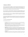
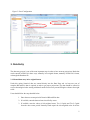
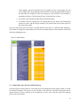
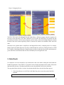
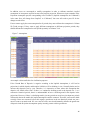
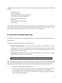
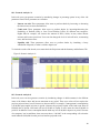
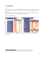
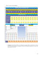
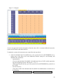
USER GUIDE
FINANCIAL PROJECTION MODEL 2.0
Murat Arslaner
The author is a Financial Sector Specialist in the Finance and Markets Global Practice of the World Bank
([email protected]). The author would like to acknowledge the significant contributions of Ines
Gonzalez Del Mazo and Farrukh Aleem Mirza in preparation of the manual. The views presented in the
paper do not necessarily represent the views of the World Bank.
1
Contents
Abbreviations and Acronyms ........................................................................................................................ 3
1. Structure of FPM 2.0 ................................................................................................................................. 4
2. Initial Excel Settings .................................................................................................................................. 6
3. Data Entry ................................................................................................................................................. 7
4. Data Mapping............................................................................................................................................ 9
5. Data Check .............................................................................................................................................. 10
6. Dash Board Settings ................................................................................................................................ 11
7. Assumptions ............................................................................................................................................ 15
8. Funds Flow and Model Balancing ........................................................................................................... 17
9. Review/Analyze the Projected Results ................................................................................................... 18
10. Scenario Analysis– % and $ ................................................................................................................... 18
11. Liquidation ............................................................................................................................................ 20
12. Present Value ........................................................................................................................................ 21
13. System-wide File ................................................................................................................................... 22
14. Trouble Shooting ................................................................................................................................... 26
15. Technical Approach to Resolving Errors in the Projections Step by Step ............................................. 27
2
Abbreviations and Acronyms
BS
CAMEL
CAR
CB
ELA
FX
FPM
LGD
PD
PLA
Balance sheet
Capital Adequacy, Asset Quality, Management Capability, Earnings, and
Liquidity
Capital adequacy ratio
Central bank
Emergency lending assistance
Foreign exchange
Financial Projection Model
Losses given default
Probability of default
Profit loss accounts
3
1. Structure of FPM 2.0
The Financial Projection Model 2.0 (FPM 2.0) is an Excel-based model composed of two types of Excel
files: the individual bank file (“BANK1.xls”) and the system-wide file (SYTEMWIDE.xls). The
individual bank file has been designed to contain the data of a single bank and allows users to analyze one
single bank at a time. The system-wide file has been designed to be linked to several individual files in
order to perform analysis of all banks at the same time (system-wide analysis).
Users will need to have as many individual files as banks they want to analyze. Alternatively, if users
have the required Excel expertise, they could create a Database file (DATABASE.XLS) that includes the
information of all the banks (each banks in a separate tab) and then link this file to an individual bank file.
In order to explain how FPM 2.0 works, it is mandatory to understand the functioning of the individual
bank files because these files will feed the system-wide file. Therefore, the explanations in this guide will
initially focus on the individual bank file.
It is also important to highlight that users must not change the names of the files, with the exception of the
individual bank file. The name of the individual bank file can be changed to names that follow the pattern
“BANK2.xls”, “BANK3.xls”, and so on, to reflect the fact that each of the files contains data for a
different bank.
1.1. Structure of the individual bank file
An individual bank file has 13 tabs:
1. User Guide: This tab gives basic step-by-step instructions on how to use the individual bank file.
2. Dash Board: This tab gives allows users to set key parameters and definitions in the banking
systems, including frequency, Capital Adequacy Ratio (CAR), and liquidity.
3. Data Entry: This tab allows users to insert data from the bank’s Balance Sheet (BS) and Profit
and Loss Account (PLA). The data can be entered in two ways: by entering the data manually; or
by linking this tab to the Database file that includes all the banks’ data.
4. Mapped Data: This tab allows users to map all the data contained in the Data Entry tab to the
FPM 2.0 financial statements format by assigning codes to the corresponding line items. After the
data are mapped, the Assumptions tab and the Calculations tab will populate. In addition, data can
be directly inserted in the Mapped Data tab by overriding its formulas. If users enter the data
directly in the Mapped Data tab, they do not have to either fill the Data Entry tab or undertake the
mapping process.
5. Assumptions: This tab calculates the implied assumptions for the BS and PLA projections using
the historical data entered in the model. Assumptions can also be manually calibrated, if required.
4
6. Calculations: This tab contains all the calculations needed to execute the projections, and
therefore is the heart of the model.
7. Funds Flow Summary: This tab calculates the Cash/Funds flow from the Operating and BS
Activities.
8. Projections: This tab shows all the projections for both the BS and PLA. The basis for these
projections can be tracked in the Calculations tab.
9. Summary and Indicators: This tab summarizes all the necessary information of the new
projected BS, PLA, and CAMELS indicators.
10. Scenario Analysis–%: This tab allows users to undertake stress tests of the bank by entering
changes in percentage points in risk factors related to interest rates, credit, exchange rates and
liquidity.
11. Scenario Analyses–$: This tab allows users to undertake stress tests of the bank by entering
changes in BS and PLA items in absolute amounts.
12. Liquidation: This tab simulates the liquidation of the bank as of the default date—or, if the bank
is projected not to default, as of the last date of the period selected as the base period for the
projections.
13. Present Value: This tab shows the present value of the bank projected over 12 periods in the
future.
Figure1. Modular Structure of the Model
5
1.2. Color coding
FPM2.0 uses the following color coding, which shows users which cells must, can, or must not be
changed:
-
Light yellow cells: Users can input data in them, but it is optional.
-
Bright yellow cells: Users must input data in them for the model to work.
-
Bright orange cells: These cells already contain formulas, but these can be overridden by users.
-
Light orange cells: These cells contain formulas that users must not change.
Figure 2. Color Coding
2. Initial Excel Settings
Before using FPM 2.0, users must configure Excel to allow for iterative and manual calculations.
Therefore, they should go to “File” tab in the Excel toolbar/“Options”/“Formulas”/”Calculation
Options”; check both “Manual Calculations” and “Enable Iterative Calculation”; and set the
“Maximum Iterations” to 200 or any other appropriate number that is higher.
These steps are mandatory for the following reasons:
-
FPM contains thousands of formulas that involve many cells whose values depend on many other
cells and circular interactions. Therefore, the Iterative Calculations function will allow Excel to
calculate each and every single formula in FPM 2.0.
-
Excel normally recalculates all formulas automatically whenever a new number is entered. The
“Manual Calculations” option allows users to calculate formulas whenever they prefer by
pressing F9. In this way, users can establish their own pace for calculations and analyze the joint
impact of changes in more than one variable. If users make changes in the cells but do not press
F9, the results of the model will not reflect those latest changes.1
1
However, it is important to note that when users save the file or close it, the changes will be saved and therefore
will be reflected in the results whenever the file is opened again.
6
Figure 3. Excel Configuration
3. Data Entry
The data entry process is one of the most important steps in order to have accurate projections. Bank data
can be entered in FPM 2.0 in three ways: manually in its original format; manually in FPM 2.0’s format;
or through the Database file.
3.1. Manual data entry in its original format
Under this option, historical data are entered directly into the Data Entry tab. At least one year of
complete BS and PLA data is required in order to get proper projections. The data should be entered in
reverse chronological order starting with data from the most recent year and filling the columns from right
to left.
Users should follow the steps detailed below:
1. Enter the most recent period of historical BS and PLA data.
2. If available, enter the data on loans classified by sector.
3. If available, enter the values of risk-weighted assets, Tier 1 Capital, and Tier 2 Capital
from the most recent period. Normally banks report the risk-weighted value for all the
7
assets together, instead of providing the risk weights of assets in percentage. For this
reason, FPM 2.0 has been designed to automatically calculate the Implied Risk Weight if
the individual risk weights for each asset category are not available. The calculation is
undertaken as follows: Risk Weighted Value of Asset/BS value of Asset.
4. If available, enter Off Balance Sheet Items and NPL dynamics.
5. If available, enter the liquidity data, the maturity data (in year terms), the floating/fixed
structure of loans, and the foreign exchange (FX) position data for the latest period of
data input in the model.
Users may notice that next to the names of the BS and PLA items, there is a column called “Mapping”.
This column is designed to assign numbers to the items in the Data Entry tab. These numbers will be used
in the Data Mapping process.
Figure 4. Manual Entry
3.2. Manual data entry directly in FPM 2.0 format
Under this option, historical data are entered directly into the Mapped Data tab using the FPM 2.0 format
for financial statements. The process to enter the data is the same one used when entering the data in
original format, with the exception of the assignments of codes, since under this option the mapping
process will not be needed.
8
3.3. Data entry through the Database file
As noted, the Database file contains the data of all banks. Users then need to link this Database file to one
individual bank file (BANK1.xls). This individual bank file will now be able to show not just the data of
Bank 1, but also the data of each of the other banks. The information of each bank can be accessed
separately (never jointly) through the Bank name parameter located in Cell A3 of the Dashboard Tab. For
example, if Bank 2 is selected in Cell A3, then the Excel sheet will show the data of Bank 2. If Bank 3 is
selected in Cell A3, then the Excel sheet will show the data of Bank 3, and so on. It is a good idea to
create a Database file, since will result less time- consuming than inputting data bank by bank.
To create a Database file, open an Excel sheet and use a different tab to include the information of each of
the banks. For example, Sheet 1 will contain all the information on Bank 1; Sheet 2 will contain all the
information on Bank 2, and so on.
The information on each bank does not need to be entered in a specific format, but the format must be
consistent across banks. The type of information needed from each of the banks is the same as that
detailed in Section 3.1, Manual data entry in its original format.
Disclaimer: While updating the Database file, users must not change the “Database file” name since FPM
2.0 will use that specific name to refer to the file.
4. Data Mapping
If users have entered the data manually in the Data Entry Tab or by using the Database file, a mapping
process is required, since FPM 2.0 calculations and projections will use only the data contained in the
Mapped Data tab. This mapping process involves the codes that were assigned to each of the different
items in the Data Entry tab.
Item-by-item users will need to identify which item in the Data Entry tab corresponds to which item in the
Mapped Data tab, as shown in Figure 5.
9
Figure 5. Mapping Process
The BS or PLA items in the Mapped Data tab might follow a different sequence than the sequences for
the items of the Data Entry Tab. These differences occur because the Data Entry tab contains the data
provided by the banks in the format used in their specific country, whereas the Mapped Data tab contains
the data in the exact format required by FPM 2.0, and the two formats can sometimes differ from each
other.
Sometimes more granular data is simplified in the Mapped Data tab by combining items. For example,
Bonds, Equities and Other Securities can all be combined under the same item, Trading Securities or Held
For Trading, of the Mapped Data tab. Simplifications are allowed when the items under consideration are
given almost the same treatment and each item individually has an insignificant value.
5. Data Check
It is imperative to review the data for any inconsistencies and errors before running the model under the
Dashboard parameters. Since FPM 2.0’s projected results are highly dependent on the quality of historical
data entered by the users, if the data inserted have errors, the projections will also be erroneous.
The steps that follow describe a few basic checks that should be done after the Data Entry process.
1. Check the indicators in cells E5-Q5 of the Data Entry tab to ensure that each of the BS is
balanced.
Total Assets = Total Liabilities + Shareholders’ Equity
10
-
If the BS is balanced, the user will see an OK in the cells E5-Q5 of the Data entry tab.
If the BS is not balanced, the user will see the amount by which assets differ from
liabilities and equity in the cells E5-Q5 of the Data entry tab.
2. Check the indicators in cells E6-Q6 of the Data Entry tab to ensure that the retained earnings
entered in the Data Entry tab are equal to the retained earnings calculated by FPM 2.0 in the
Mapped Data tab.
- If both are equal, the user will see OK in cells E6-Q6 of the Data entry tab.
- If both are not equal, the user will see the amount by which they differ in cells E6-Q6 of
the Data entry tab.
3. Check the assigned codes at the Data entry tab and the Mapped Data tab to verify that they
are equal for the same items.
4. Run the model once and check for:
- Unexpected steep increases/decreases in consecutive years of historical data
- Zero or negative values of certain items that are expected to be positive (such as . loans,
provisions, or any other BS asset)
- Differences between the stock of provisions in the BS and the flow provisions on PLA that
can be explained
- Exaggerated capital adequacy ratios
- Risk weighted assets greater than 100 percent of the actual value.
Disclaimer: The list above provides only very basic and highly recurrent errors; it is not an exhaustive list.
6. Dash Board Settings
After reviewing the data for accuracy and reliability, the next step is to set the projection parameters in
the Dashboard Tab. All parameters should be filled up; however, their values can be changed at any time
during the process.
11
Figure 6. Dash Board Settings
Name of the Bank (Cell A3)
This parameter allows users to elect the bank for which they would like to run the model by using the
drop down menu to select the bank name. Once the bank is selected, users need to Press F9 to run the
model. FPM 2.0 will update all the projections based on the data for the selected bank.
FPM 2.0, which includes the usage Database file among its functionalities, now allows changing the
information of the bank in the spread sheet just by changing the name of the bank in Cell A3.
Base Date of Historical Data/Period 0 (Cell B3)
This parameter determines the data used to calculate projections. Since the data for the projections must
be from the most recent period, users must enter the date of the most recent period for which they have
data in Cell B3, using the following format: MM/DD/YYYY.
Frequency of Projections (Cells C3–N3)
Users can change the frequency of the projections by using the drop down lists in Cells C3 toN3.Users
can choose from daily, weekly, monthly, quarterly, semi-annual, or annual frequency.
Although it is possible to select different frequencies for different projection periods, it is recommended
that, for purposes of consistency and fair comparison, users select equal frequencies for projection
periods.
12
Frequency of Historical Data (Cell A5)
Users can determine the frequency of the historical data used through the drop down list in Cell A5. The
drop down includes six different frequencies: annual, semi-annual, quarterly, monthly, weekly, and daily.
Number of Periods of Historical Data (Cell B5)
This parameter corresponds to the number of periods the user would want to take into account for the
calculation of the implied assumptions. This number will always be one unit less than the actual number
of periods. For example, if users have data for only two periods (the base year and year prior to the base
year), users must input 1 in Cell B5 as the Number of Periods of Historical Data.
Minimum Regulatory CAR (Cell C5)
The Minimum Regulatory CAR indicates the percentage of capital with which any bank needs to comply.
FPM 2.0 will use this number as a threshold to determine when a bank defaults and cannot continue with
its activities. The percent threshold varies from country to country, and therefore can be adjusted by the
user in Cell C5.
Minimum Tier 1 Ratio (Cell D5)
The Minimum Tier 1 Ratio indicates the percentage of Tier 1 capital with which any bank needs to
comply. FPM 2.0 will use this number as a threshold to determine when a bank defaults and cannot
continue with its activities.
Minimum Core Tier 1 Ratio (Cell E5)
The Minimum Core Tier 1 Ratio indicates the percentage of core Tier 1 capital with which any bank
needs to comply. FPM 2.0 will use this number as a threshold to determine when a bank defaults and
cannot continue with its activities.
Funding Liquidity Risk (Cell F5)
The funding liquidity risk parameter is used to simulate a liquidity shortage resulting from the suspension
of lending activities by other financial institutions in the capital market. If users activate it by choosing
“YES,” whenever any bank’s CAR falls below the Threshold CAR for Funding Liquidity Risk (Cell G5),
capital market activities with that particular bank will stop, negatively affecting the bank’s liquidity. If
users choose “NO,” capital markets activities will continue as usual.
Threshold CAR for Funding Liquidity Risk (Cell G5)
The threshold for funding liquidity risk is the CAR below which capital market activities of a bank will
stop. This threshold is normally a few percentage points higher than the Minimum Regulatory CAR
because it indicates the confidence level of the investors with the bank. This confidence level starts to
decrease when the CAR of the bank approaches the minimum requirement. Users can determine this
threshold in Cell F5.
Market Liquidity Risk (Cell H5)
13
This parameter determines whether there is a sale of securities in the bank (Net Securities Held for
Trading, and Available for Sale Securities) when the bank itself suffers from a shortage in liquidity. If
users select “YES,” the bank will sell securities until the shortage is covered. If users select “NO,” the
bank will not sell securities to cover the shortage.
Whenever the sale of all securities is insufficient to cover the shortage, Emergency Lending Assistance
(ELA) from the central bank is automatically injected in the bank.
Loss Rate on Fire Sale of Securities (Cell I5)
Whenever securities are sold for an urgent need, such as a liquidity shortage emergency, they are sold
normally at a discount. If historical data are available, users can enter a fixed percentage in Cell I5 as an
assumed Loss Rate on Fire Sales of Securities.
Repricing Data in Use (Cell K5)
This parameter determines whether FPM 2.0 calculates the repricing of the data in the projections. This
repricing would include the maturing of loans and the generation of new loans according to historical
rates of interest rate evolution, maturity, and fixed/floating structure.
Cap on Interest Rate Assumptions (Cell L5)
This is the maximum interest rate for interest-earning assets and interest-bearing liabilities. It serves as a
tool to counter negative rates implied due to any data errors or volatility. By default, FPM 2.0 will use the
interest rate implied from historical data; otherwise, users can set a different rate in Cell L5. Whenever
the implied rate is higher than the cap rate, the model will use the cap rate.
Cap on Growth Rate Assumptions (Cell M5)
Since some items in the balance sheet could have increased or decreased at unusual rates in the past, FPM
2.0 incorporates a cap on growth rate assumptions to avoid unrealistic projections. In case the historical
growth rates are too high or too low, this cap will keep the growth rate within reasonable limits.
Loan Projections Based on NPL Evolution Data (Cell N5)
This parameter determines whether loans will be projected based on additional information on default,
restructuring, write-off, and foreclosed rates instead of based on the rates FPM calculates from the BS and
PLA historical data.
FPM 2.0 runs loan projections based on two different sets of data: balance sheet data only; or balance
sheet data, together with other information on NPL evolution (write-offs, restructurings, and
foreclosures). A simplified approach uses only balance sheet data (performing and nonperforming loans)
to calculate the implied assumptions, which are the default rates and the restructuring rates. A more
complex approach involves the data available on the evolution of NPLs, such as restructured NPLs,
written-off NPLs, and foreclosed NPLs. This more complex approach is activated when users activate the
parameter, “Loan Projections Based on NPL Evolution Data.”
Contagion (Cell N5)
14
This parameter controls for a contagion effect among banks whenever one bank fails. If the option
selected is “YES,” the impact of a bank failure will be reflected in the projections of all other banks. If a
defaulted bank has net interbank liabilities at the time of failure, this amount will be allocated to each
bank as loss in proportion to their lending in the interbank market in the following period. In addition, if
the failed bank has net interbank assets at the time of failure, the failure will provoke a reduction of
interbank assets, which in return will lead to a reduction of the level of lending in other banks in the next
period.
7. Assumptions
Realistic/reasonable assumptions by users are essential to get realistic/reasonable assumptions in FPM
2.0. Even though the best way to improve results may be to increase the quality or granularity of the data,
further clarification is not always possible. Therefore, the Assumptions tab allows assumptions to be
adjusted for more realistic projections.
This tab contains three main parts:
-
Column C: Shows the list of BS and PLA items and indicates the rate based on which each BS
item (Column C) is projected each period. For example, cash grows based on the percentage of
deposits, while property, plant, and equipment grow based on a percentage growth rate. Assets—
mostly interest-earning ones, for which no such rates/ratios are calculated— are basically
dependent upon the Allocation of Funds Flow available within the bank.
-
Columns F–R: Show the Implied Assumptions of each item in each period that are calculated
by the model in order to generate the projections. The cells in this part of the Excel sheet should
not be altered, as they are automatically calculated from the historical data located in the Mapped
Data tab. The values shown in these cells are annualized regardless of the frequency of the data
entered or the projections wanted. 2
-
Columns W–AI: Show the Projection Assumptions that can be changed by users at will. These
cells contain formulas that can be overridden, but must be set back again later. The
values/formulas inserted in these cells must be annualized rates regardless of the frequency of the
data entered or the projections wanted.
Users must review the implied assumptions for BS and PLA projections. In addition, it is highly
recommended for users to review the implied assumptions for capital (CAR), liquidity, the maturity and
fixed/floating structure of assets, and the foreign exchange positions in order to improve the accuracy of
results.
2
Later, the model will make the necessary conversions for the projections to be shown in the frequency desired by
the user.
15
In addition, users are encouraged to modify assumptions in order to calibrate unrealistic implied
assumptions or incorporate expected events to the baseline projection. When users input a number in the
Projection Assumption part, the corresponding cell of Column U (Implied Assumptions Are Calibrated?)
in the same lines will change from “Implied” to “Calibrated,” but users still need to press F9 for the
changes to take effect.
If users want to apply the same assumption for all periods, they must calibrate the assumption in Column
W (Trend average). If they want to apply different assumptions to different projection periods, they
should calibrate the assumption for each period separately in Columns Y–AJ.
Figure 7. Assumptions
An example is discussed below for clarification purposes.
If the Growth Rate of Deposits is negative according to the Implied Assumptions, it will lead to
projections in which deposits and therefore liabilities will be shrinking in size. Normally banks tend to
increase their deposits year by year. Therefore, it is imperative to know where this assumption that
deposits will shrink comes from. If there is a continuous declining trend in the deposits for 5 or 6
consecutive historical periods, then it is understandable to have a declining trend in the deposits in the
projections. However, if there is a declining trend in just two periods or users have just input two periods
of historical data in the model, this implied assumption could be erroneous. Therefore, users need to think
critically if there are reasons to believe this negative growth rate in the two historical periods was just a
one-off event or an actual trend. If it was a one-off event, users should manually calibrate the growth rate
of deposits in the Projection Assumptions part by inserting a more realistic growth rate.
16
Although the rate of growth of every BS and PLA item is important, the rates of some items need more
attention:
-
Growth of deposit
Probability of default
Loss given default or specific provision ratio
Work out ratio or loan restructuring ratio
Charge off or loan written off ratio
Interest rates
Gains and losses rates on securities
Dividend rates.
The assumption rates are used by FPM 2.0 in the Calculations tab, which also uses values from and feeds
values to the Funds Flow Summary tab. Both tabs must not be modified by the users (unless a systemwide analysis is undertaken; see Section 13. System-wide File for more information).
8. Funds Flow and Model Balancing
The Funds Flow Statement is the tool that balances the model, creating an interplay among all the items in
the BS and PLA.
This interplay generates two basic types of Funds Flow (FF):
-
Balance Sheet Funds Flow: These flows come from “Investing” and “Financing” Activities in
the balance sheet. In general, Investing Activities are defined as those activities that use funds,
while Financing Activities are defined as those activities that generate the funds themselves and
therefore, are the sources of funds.
-
Operational Cash Flow: These flows come from operations or profit and loss accounts.
Operating Activities can generate and use funds.
Final Funds Flow Available = Balance Sheet Funds Flow + Operational Cash Flow
The Final Funds Flow Available can be positive or negative. If positive, the Final Funds Flow Available
will be allocated among different assets (loans, securities, and interbank assets) in the future periods,
following past historical trends. If negative, the model will follow these steps to meet the short fall:
1. Reduction of central bank and interbank assets
2. Sale of securities, if the sale of securities option has been activated in the Dashboard tab. The
model will first sell Held for Trading Securities and later Available for Sale Securities.
3. The remainder will be covered by the central bank ELA (Emergency Liquidity Assistance)
facility until the BS is balanced.
17
9. Review/Analyze the Projected Results
Once users have confirmed that the funds flows are correct, they may proceed by pressing F9 to run the
model. A baseline projection will be automatically generated based on the Implied and Projected
Assumptions. This baseline projection will be shown in two tabs:
-
The Projections tab, which includes the projections of each BS and PLA item.
-
The Summary and Indicators tab, which includes the projections of only the main BS and PLA
items, together with viability and performance indicators (CAMELs). In addition, if the bank
needs external additional capital and/or liquidity, this tab shows the amount required in each of
the projected periods.
Users must review the results before taking any further action in the model. First, they must check that the
base period data is the one they intended. Second, they must check that all changes among consecutive
future projections are smooth, if they all are set for the same frequency. In addition, other important items
to be reviewed are:
1. Whether Projected BSs are balanced
2. Whether total assets and net profit (loss) change smoothly from period to period
3. Whether projected CARs in the Summary and Indicators tab are in line with common sense
expectations. If there are divergences between users’ common sense expectations and actual
FPM 2.0 results, users need to investigate if those divergences are justified by the Implied
Assumptions, and whether those Implied Assumptions need to be calibrated.
10. Scenario Analysis– % and $
Until now, FPM 2.0 has provided users with a baseline scenario that reflects the behavior of the bank
under what users consider a plausible future. However, FPM 2.0 also includes the functionality of
scenario analysis whose main purpose is to perform stress tests.
FPM 2.0 Scenario Analysis tabs allows users to study the impact of a specific shock, not just on the
capitalization of a bank (CAR), but also on other items, such as different incomes, NPLs, and provisions.
To check the results of the shocks, users must press F9 and go to the Projections and the Summary and
Indicators Tab. Users once again must ensure that the results shown are coherent with the stress scenario
inserted.
As part of the scenarios, users may also want to modify certain parameters in the Dashboard tab. For
example, users could activate/deactivate market liquidity risk or change the threshold CAR for funding
liquidity risk.
FPM 2.0 has two tabs dedicated to Scenario Analysis: Scenario Analysis–%, and Scenario Analysis–$.
18
10.1. Scenario Analysis– %
In this tab, users can generate scenarios by introducing changes in percentage points in any of the risk
parameters listed. Those parameters are related to:
-
Interest rate risk: These parameters allow users to perform shocks by increasing or decreasing
the interest rates on assets and liabilities.
-
Credit risk: These parameters allow users to perform shocks by increasing/decreasing the
Probability of Defaults (PDs) or Loss Given Defaults (LGDs) for different loan categories.
Higher PDs for example, will increase the amount of NPLs, which, in turn, reduce interest
incomes and increase provisions. Users can also change the level of write-off ratios, restructuring
rates, and foreclosure rates.
-
Liquidity risk: These parameters allow users to perform shocks by simulating a heavy
withdrawal of deposits, or what is called a deposit run.
To check the results of the shocks, users must check the Projections and the Summary and Indicators Tab.
Figure 8. Scenario Analysis-%
10.2. Scenario Analysis–$
In this tab, users can also generate scenarios by introducing changes in dollar amounts in the different
items of the balance sheet and income statement at any period. These new values will not replace the
previous projected ones, but will increase or decrease them. For example, if management is contemplating
a $100,000 equity/capital injection in period 4 because the projected capital of the bank went down to
$50,000, then in period 4 the bank will have $150,000 of capital if users insert the value $100,000 in
period 4. In addition if users contemplate that the bank may lose $100,000 in deposits in period 3 because
of a temporary lost in confidence, then users must insert “-100,000” in the corresponding cell so that the
model subtracts $100,000 from the previous baseline projected result.
19
11. Liquidation
FPM 2.0 provides an option to calculate the liquidation value of a bank as of its default date—or, if the
bank is projected not to default, as of the last date of the period selected as the base period for the
projections. 3
In this tab, users must introduce the expected loss rate of each of the balance sheet and off-balance sheet
items 4 at the base period, as well as the insured and covered liabilities.
Figure 9. Net Asset Recovery
In addition, users may want to add the resolution costs and valuation of tangible and intangible assets to
the calculation.
3
4
As mentioned, the base period tends to be the latest period available for which users have data.
This expected loss rate should be based in a historical analysis previously made by the users.
20
Figure10. Resolution Costs
With all this information, the model will calculate the Net Asset Value of the bank when users press F9.
12. Present Value
FPM 2.0 allows users to project the present value of a bank over the future. The model discounts the Net
Profit after Taxes values and the required additions to capital calculated in the projections at the implied
rate calculated by the model. The result is shown in line 11 as “Present Value of DAD.”
Users can customize these calculations by adding additional capital investments or by changing the
discount rates. To see the results of the customized calculations, users must press F9.
21
Figure 11. Present Value
13. System-wide File
FPM 2.0 can be used to analyze a whole banking system if users complement the individual bank files
with the system-wide file. This latter file, if linked with the individual bank files, allows users to
undertake a system-wide risk assessment considering the interconnectedness among the banks.
This file contains three tabs:
-
User Guide: This tab gives basic step-by step instructions on how to use the individual bank file.
-
Dashboard: This tab contains three main sections:
•
Parameters Section: This part is the same and has the same functionality as the one
contained in the individual banks file Dashboard, with the exception of the Name of the
Banks Cell. Cell A3, which contains the text “ALL BANKS,” must not be changed.
•
Scenario Analysis Section: This part is the same and has the same functionality as the
Scenario Analysis-% Tab of the individual banks file. However, in this case, any
percentage changes made in the risk factors of this section of the system-wide file will
affect all individual bank files at the same time.
•
Projection Results Section: This part shows the results of the system-wide analysis in
three graphs: Summary results, Defaulted bank and their names, and CAMEL Indicators.
The summary results figure and the CAMEL indicator figure have drop down menus for
users to determine which item/indicator is shown in each of the graphs.
22
Figure 12. System-wide Dash Board
-
Contagion: This tab allows FPM 2.0 to calculate the contagion effect of a bank failure. This tab
works only when the parameter Contagion is activated in all individual banks files as well as the
system-wide file (Cell N5).
23
Figure 13. Contagion
As users can appreciate from the descriptions of the tabs, there will be a constant feedback between the
system-wide file and the individual bank files.
To undertake a system-wide assessment, users must follow the steps below:
1. Link the individual bank file (BANK1.xls) to the system-wide file (SYSTEMWIDE.xls) by
linking each of the yellow cells in the Dashboard, Scenario Analysis–%, and Summary and
Indicators tabs of both files:
- Open both files.
- Go to the individual bank file (BANK1.xls) Dashboard; click on Cell B3, which contains the
base date assigned by the user, and write an “=” or a “+”.
- Without pressing the enter key, go to the system-wide file (SYSTEMWIDE.xls), and click on
the Cell B3.
- Press the enter key.
- Check that Cell B3 of the individual bank file (BANK1.xls) Dashboard has a formula such as
the following:
=[SYSTEMWIDE.xls]DashBoard!$B$3 or +[SYSTEMWIDE.xls]DashBoard!$B$3”
24
-
Repeat the process with each of the yellow cells of the Dashboard. with the exception of Cell
A3, which contains the name of the bank.
Repeat the process with each of the Scenario Analysis–% and Summary and Indicators tabs.
2. Link the Calculations tab of the individual bank file (BANK1.xls) to the Contagion tab of the systemwide file (SYSTEMWIDE.xls) by following these steps:
- Go to the individual bank file (BANK1.xls) Calculations tab.
- In the section that includes BS data, replace the formula contained in the Due to Banks cell
from base period 0 (Cell F81) with the following one:
=+IF(DashBoard!$N$5="Yes",IFERROR(VLOOKUP(DashBoard!$A$3,
INDIRECT("[SYSTEMWIDE.xls]Contagion!c515:R614"),4+G2,0),0),
F81*(1+G438)+'ScenarioAnalysis$'!G81*1)
-
Copy Cell G81 (not its formula!) and paste it in Cells H81 to N81.
Check that the cells have formulas that follow this pattern below:
• Cell H81 must now contain:
=+IF(DashBoard!$N$5="Yes",IFERROR(VLOOKUP(DashBoard!$A$3,
INDIRECT("[SYSTEMWIDE.xls]Contagion!c515:R614"),4+H2,0),0),
G81*(1+H438)+'ScenarioAnalysis$'!H81*1)
• Cell I81 must now contain:
=+IF(DashBoard!$N$5="Yes",IFERROR(VLOOKUP(DashBoard!$A$3,
INDIRECT("[SYSTEMWIDE.xls]Contagion!c515:R614"),4+I2,0),0),
H81*(1+I438)+'ScenarioAnalysis$'!I81*1)
-
In the same Calculations tab, look for the section that includes Income Statement data, and
replace the formula contained in the Extraordinary Incomes (Expenses) cell from base period
0 (Cell F197) with the following one:
=+IF(DashBoard!$N$5="Yes",IFERROR(VLOOKUP(DashBoard!$A$3,INDIRECT("[S
YSTEMWIDE.xls]Contagion!C311:R410"),4+G2,0),0),0)+'ScenarioAnalysis$'!G143*1
-
-
Copy Cell F197 (not its formula!) and paste it in Cells H197 to N197.
Check that the cells have formulas that follow this pattern below:
• Cell H197 must now contain:
=+IF(DashBoard!$N$5="Yes",IFERROR(VLOOKUP(DashBoard!$A$3,INDIRECT
("[SYSTEMWIDE.xls]Contagion!C311:R410"),4+H2,0),0),0)+'ScenarioAnalysis$'!
H143*1
• Cell I197 must now contain:
=+IF(DashBoard!$N$5="Yes",IFERROR(VLOOKUP(DashBoard!$A$3,INDIRECT
("[SYSTEMWIDE.xls]Contagion!C311:R410"),4+I2,0),0),0)+'ScenarioAnalysis$'!I1
43*1
Save the individual bank file (BANK1.xls) under the same folder as the system-wide file
(SYSTEMWIDE.xls).
25
3.
Add more banks to the system:
- Make copies of the individual bank file (BANK1.xls), and rename them as BANK2.xls,
BANK3.xls, and so on.
- Replace the information on the Data Entry/Mapped Data tabs to reflect the information of
each of the other banks, and select the name of the bank on the Dashboard tab. Rather than
inputting data manually into each individual bank file, a Database file with the data of all
individual banks can be created. The Database file can be then linked to an empty individual
bank file (BANK1.xls) so that the data are imported automatically from the Database file to
the individual bank file upon the selection of the Bank`s name on the Dashboard tab. If users
prefer to create a Database file, it should be done before making copies of the original
individual bank file (BANK1.xls) to create the files for other banks.
Once users have saved the information of each bank in different individual files (BANK1.xls,
BANK2.xls, BANK3.xls…), they should open all of these individual files one by one, together with the
system-wide file. For any system-wide analysis to work, all files must be open.
Users can now proceed to change parameters in the yellow cells of the Dashboard tab of the system-wide
file located in each of the three sections of this tab (Dashboard parameters, Scenario Analysis, and
Projection Results-Summary and Indicators). Once the desired changes are made, users must press F9 for
FPM 2.0 to calculate. (Generally results will be generated in a little less than a minute on a system with
sufficient RAM and a speedy processor.)
14. Trouble Shooting
Listed below are some common problems/errors users may encounter while using FPM 2.0:
-
-
Review if the base year’s reported and mapped net profits are equal. Otherwise, revise the
data entry and the mapped entry tabs for errors and review the formulas in the Projections tab.
Review if the base year’s assets are equal to the liabilities and shareholder’s equity together.
Otherwise, revise the data entry and the mapped entry tabs for errors and review the formulas
in the Projections tab.
Review whether Funds Flow is balanced in each of the projection periods. Otherwise, check
the calculation of funds flow to ensure that all eligible items have been taken into account.
Review for Excel errors such as NUM, DIV/0, REF, and the like. Check the Excel Help
manual to understand the specific circumstances under which these errors appear. For
example, NUM error occurs when any of the input cells has a value that is not numeric.
DIV/0 occurs when some number in the formula is divided by zero in the formula. REF
occurs when one of the input/referred cells is missing (it might have been accidentally
deleted).
26
-
Check for aggregate line items with irregular projection trends, such as increases/decreases at
unrealistic rates. To determine where the problem is, review whether the formulas are correct
and the data have been entered properly. Then review the corresponding assumption(s) and,
when necessary, recalibrate the problematic assumption(s) to get a realistic or reasonable
projection.
15. Technical Approach to Resolving Errors in the Projections
Step by Step
Whenever users get errors in the projections, the first thing they need to do is to understand where the
error starts. In order to look for the origin of the problem, users may follow the steps listed below:
1. Close the model without saving it and reopen it.
2. Set the Iterative Calculations to 1 (instead of 200, or any other number the user entered
previously).
3. Press F9 and check if any error appears on the balance sheet or income statement in the
Calculations tab.
4. Repeat the process until the first error appears.
5. Note the cell that shows the error.
6. Close the file without saving it again.
7. Reopen the file and fix the error before pressing F9 again.
8. To fix the error, users may want to use the Trace Precedents Excel function, which can be
found under the Formulas menu of the Quick Access Toolbar, to figure out where the error
cell is taking the values from. In addition, users may want to use the Evaluate Formula Excel
function under the Formulas menu of the Quick Access Toolbar to try to see which particular
values are responsible for the error.
9. Once the identified error is fixed, change the Iterative Calculations to 200 again and review
the Calculations tab for more errors. If more errors appear, repeat the process.
27