Download Model-Driven Development and Simulation of - Hu

Model-Driven Development and Simulation of
Distributed Communication Systems
DISSERTATION
zur Erlangung des akademischen Grades
Dr. Rer. Nat.
im Fach Informatik
eingereicht an der
Mathematisch-Naturwissenschaftlichen Fakultät II
Humboldt-Universität zu Berlin
von
M.Sc. Mihal Brumbulli
Präsident der Humboldt-Universität zu Berlin:
Prof. Dr. Jan-Hendrik Olbertz
Dekan der Mathematisch-Naturwissenschaftlichen Fakultät II:
Prof. Dr. Elmar Kulke
Gutachter:
1. Prof. Dr. Joachim Fischer
2. Prof. Dr. Klaus Bothe
3. Prof. Dr. Andreas Prinz
eingereicht am: 27.03.2014
Tag der mündlichen Prüfung: 17.03.2015
To my family
Abstract
Distributed communication systems have gained a substantial importance over the past
years with a large set of examples of systems that are present in our everyday life. The
heterogeneity of applications and application domains speaks for the complexity of
such systems and the challenges that developers are faced with. The focus of this dissertation is on the development of applications for distributed communication systems.
There are two aspects that need to be considered during application development. The
first and most obvious is the development of the application itself that will be deployed
on the existing distributed communication infrastructure. The second and less obvious, but equally important, is the analysis of the deployed application. Application
development and analysis are like “two sides of the the same coin”. However, the separation between the two increases the cost and effort required during the development
process. Existing technologies are combined and extended following the model-driven
development paradigm to obtain a unified development method. The properties of the
application are captured in a unified description which drives automatic transformation
for deployment on real infrastructures and/or analysis. Furthermore, the development
process is complemented with additional support for visualization to aid analysis. The
defined approach is then used in the development of an alarming application for earthquake early warning.
Zusammenfassung
Verteilte Kommunikationssysteme haben in den letzten Jahren enorm an Bedeutung
gewonnen, insbesondere durch die Vielzahl von Anwendungen in unserem Alltag. Die
Heterogenität der Anwendungen und Anwendungsdomänen spricht für die Komplexität solcher Systeme und verdeutlicht die Herausforderungen, mit denen ihre Entwickler
konfrontiert sind. Der Schwerpunkt dieser Arbeit liegt auf der Unterstützung des Entwicklungsprozesses von Anwendungen für verteilte Kommunikationssysteme. Es gibt
zwei Aspekte, die dabei berücksichtigt werden müssen. Der erste und offensichtlichste ist die Unterstützung der Entwicklung der Anwendung selbst, die letztendlich auf
der vorhandenen verteilten Kommunikationsinfrastruktur bereitgestellt werden soll.
Der zweite weniger offensichtliche, aber genauso wichtige Aspekt besteht in der Analyse der Anwendung vor ihrer eigentlichen Installation. Anwendungsentwicklung und
-analyse sind also “zwei Seiten der gleichen Medaille”. Durch die Berücksichtigung beider Aspekt erhöht sich jedoch andererseits der Aufwand bei der Entwicklung. Die Arbeit kombiniert und erweitert vorhandene Technologien entsprechend dem modellgetriebenen Entwicklungsparadigma zu einer einheitlichen Entwicklungsmethode. Die
Eigenschaften der Anwendung werden in einer vereinheitlichten Beschreibung erfasst,
welche sowohl die automatische Überführung in Installationen auf echten Infrastrukturen erlaubt, als auch die Analyse auf der Basis von Modellen. Darüber hinaus wird der
Entwicklungsprozess mit zusätzlicher Unterstützung bei der Visualisierung der Analyse ergänzt. Die Praktikabilität des Ansatzes wird anschließend anhand der Entwicklung
und Analyse einer Anwendung zur Erdbebenfrühwarnung unter Beweis gestellt.
Contents
1
Introduction
1.1 Problem Statement
1.2 Approach . . . . .
1.3 Hypothesis . . . .
1.4 Contributions . . .
1.5 Structure . . . . . .
.
.
.
.
.
.
.
.
.
.
.
.
.
.
.
.
.
.
.
.
.
.
.
.
.
.
.
.
.
.
.
.
.
.
.
.
.
.
.
.
.
.
.
.
.
.
.
.
.
.
.
.
.
.
.
.
.
.
.
.
.
.
.
.
.
.
.
.
.
.
.
.
.
.
.
1
2
3
3
3
4
2
Background
2.1 What is a Model? . . . . . . . . . . . . . . .
2.1.1 Software Models . . . . . . . . . . .
2.2 Model-Driven Development . . . . . . . . .
2.2.1 Model-Driven Software Development
2.3 Simulation . . . . . . . . . . . . . . . . . . .
2.3.1 Discrete Event Simulation . . . . . .
2.3.2 Simulation of Software Systems . . .
2.4 Visualization . . . . . . . . . . . . . . . . .
.
.
.
.
.
.
.
.
.
.
.
.
.
.
.
.
.
.
.
.
.
.
.
.
.
.
.
.
.
.
.
.
.
.
.
.
.
.
.
.
.
.
.
.
.
.
.
.
.
.
.
.
.
.
.
.
.
.
.
.
.
.
.
.
.
.
.
.
.
.
.
.
.
.
.
.
.
.
.
.
.
.
.
.
.
.
.
.
.
.
.
.
.
.
.
.
.
.
.
.
.
.
.
.
.
.
.
.
.
.
.
.
5
5
6
7
8
9
10
11
11
3
Related Work
3.1 Modeling Languages . . . . . . . . . . . .
3.1.1 LOTOS . . . . . . . . . . . . . . .
3.1.2 Estelle . . . . . . . . . . . . . . . .
3.1.3 UML . . . . . . . . . . . . . . . .
3.1.4 SDL . . . . . . . . . . . . . . . . .
3.1.5 Outlook . . . . . . . . . . . . . . .
3.2 Simulation . . . . . . . . . . . . . . . . . .
3.2.1 ns-2 . . . . . . . . . . . . . . . . .
3.2.2 ns-3 . . . . . . . . . . . . . . . . .
3.2.3 OMNeT++ . . . . . . . . . . . .
3.2.4 OPNET . . . . . . . . . . . . . . .
3.3 Model-Driven Development and Simulation
3.3.1 MDD with UML . . . . . . . . . .
3.3.2 MDD with SDL . . . . . . . . . .
3.3.3 Outlook . . . . . . . . . . . . . . .
3.4 Visualization . . . . . . . . . . . . . . . .
3.5 Conclusion . . . . . . . . . . . . . . . . .
.
.
.
.
.
.
.
.
.
.
.
.
.
.
.
.
.
13
13
14
15
16
18
20
22
22
23
26
27
28
28
32
36
38
39
.
.
.
.
.
.
.
.
.
.
.
.
.
.
.
.
.
.
.
.
.
.
.
.
.
.
.
.
.
.
.
.
.
.
.
.
.
.
.
.
.
.
.
.
.
.
.
.
.
.
.
.
.
.
.
.
.
.
.
.
.
.
.
.
.
.
.
.
.
.
.
.
.
.
.
.
.
.
.
.
.
.
.
.
.
.
.
.
.
.
.
.
.
.
.
.
.
.
.
.
.
.
.
.
.
.
.
.
.
.
.
.
.
.
.
.
.
.
.
.
.
.
.
.
.
.
.
.
.
.
.
.
.
.
.
.
.
.
.
.
.
.
.
.
.
.
.
.
.
.
.
.
.
.
.
.
.
.
.
.
.
.
.
.
.
.
.
.
.
.
.
.
.
.
.
.
.
.
.
.
.
.
.
.
.
.
.
.
.
.
.
.
.
.
.
.
.
.
.
.
.
.
.
.
.
.
.
.
.
.
.
.
.
.
.
.
.
.
.
.
.
.
.
.
.
.
.
.
.
.
.
.
.
.
.
.
.
.
.
.
.
.
.
.
.
.
.
.
.
.
.
.
.
.
.
.
.
.
.
.
.
.
.
.
.
.
.
.
.
.
.
.
.
.
.
.
.
.
.
.
.
.
.
.
.
.
.
.
.
.
.
.
.
.
.
.
.
.
.
.
.
.
.
ix
Contents
4
Modeling
4.1 Specification and Description Language – Real Time
4.1.1 A Client-Server Application . . . . . . . . .
4.1.2 Architecture . . . . . . . . . . . . . . . . . .
4.1.3 Communication . . . . . . . . . . . . . . .
4.1.4 Behavior . . . . . . . . . . . . . . . . . . . .
4.1.5 Object Orientation . . . . . . . . . . . . . .
4.1.6 Deployment . . . . . . . . . . . . . . . . . .
4.2 Extensions . . . . . . . . . . . . . . . . . . . . . . .
4.2.1 Communication . . . . . . . . . . . . . . .
4.2.2 Deployment . . . . . . . . . . . . . . . . . .
4.3 Conclusion . . . . . . . . . . . . . . . . . . . . . .
5
Automation
5.1 State-of-the-art . . . . . . . . . . . . . . . .
5.1.1 System Development Tools . . . .
5.1.2 Interfaces and Code Transformation
5.2 Code Generation . . . . . . . . . . . . . .
5.2.1 Architecture and Behavior . . . . .
5.2.2 Communication . . . . . . . . . .
5.2.3 Deployment . . . . . . . . . . . . .
5.3 Conclusion . . . . . . . . . . . . . . . . .
6
Visualization
6.1 Tracing . . . . . . . . . . . . . . . .
6.1.1 Node Events . . . . . . . . .
6.1.2 Network Events . . . . . . .
6.1.3 Trace Generation and Format
6.2 Trace Visualization . . . . . . . . . .
6.2.1 Front-End . . . . . . . . . . .
6.2.2 Back-End . . . . . . . . . . .
6.3 Conclusion . . . . . . . . . . . . . .
.
.
.
.
.
.
.
.
.
.
.
.
.
.
.
.
.
.
.
.
.
.
.
.
.
.
.
.
.
.
.
.
.
.
.
.
.
.
.
.
.
.
.
.
.
.
.
.
.
.
.
.
.
.
.
.
.
.
.
.
.
.
.
.
.
.
.
.
.
.
.
.
7
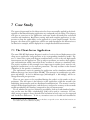
Case Study
7.1 The Client-Server Application . . . . . . . . . . . .
7.2 Alarming Application for Earthquake Early Warning
7.2.1 Earthquakes and Early Warning . . . . . . .
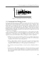
7.2.2 Earthquake Early Warning Systems . . . . .
7.2.3 SOSEWIN . . . . . . . . . . . . . . . . . .
7.2.4 The Alarming Protocol . . . . . . . . . . . .
7.2.5 Application Scenario . . . . . . . . . . . . .
7.3 Conclusion . . . . . . . . . . . . . . . . . . . . . .
.
.
.
.
.
.
.
.
.
.
.
.
.
.
.
.
.
.
.
.
.
.
.
.
.
.
.
.
.
.
.
.
.
.
.
.
.
.
.
.
.
.
.
.
.
.
.
.
.
.
.
.
.
.
.
.
.
.
.
.
.
.
.
.
x
.
.
.
.
.
.
.
.
.
.
.
.
.
.
.
.
.
.
.
.
.
.
.
.
.
.
.
.
.
.
.
.
.
.
.
.
.
.
.
.
.
.
.
.
.
.
.
.
.
.
.
.
.
.
.
.
.
.
.
.
.
.
.
.
.
.
.
.
.
.
.
.
.
.
.
.
.
.
.
.
.
.
.
.
.
.
.
.
.
.
.
.
.
.
.
.
.
.
.
.
.
.
.
.
.
.
.
.
.
.
.
.
.
.
.
.
.
.
.
.
.
.
.
.
.
.
.
.
.
.
.
.
.
.
.
.
.
.
.
.
.
.
.
.
.
.
.
.
.
.
.
.
.
.
.
.
.
.
.
.
.
.
.
.
.
.
.
.
.
.
.
.
.
.
.
.
.
.
.
.
.
.
.
.
.
.
.
.
.
.
.
.
.
.
.
.
.
.
.
.
.
.
.
.
.
.
.
.
.
.
.
.
.
.
.
.
.
.
.
.
.
.
.
.
.
.
.
.
.
.
.
.
.
.
.
.
.
.
.
.
.
.
.
.
.
.
.
.
.
.
.
.
.
.
.
.
.
.
.
41
41
41
42
45
45
51
52
53
53
58
63
.
.
.
.
.
.
.
.
65
65
66
70
72
73
93
102
109
.
.
.
.
.
.
.
.
.
.
.
.
.
.
.
.
111
111
112
114
115
115
116
119
121
.
.
.
.
.
.
.
.
.
.
.
.
.
.
.
.
123
123
125
125
129
130
133
137
142
.
.
.
.
.
.
.
.
.
.
.
.
.
.
.
.
.
.
.
Contents
8
Conclusions
8.1 Hypothesis . . . . .
8.2 Contributions . . . .
8.3 Future Work . . . .
8.3.1 Modeling . .
8.3.2 Automation .
8.3.3 Visualization
.
.
.
.
.
.
.
.
.
.
.
.
.
.
.
.
.
.
.
.
.
.
.
.
.
.
.
.
.
.
.
.
.
.
.
.
.
.
.
.
.
.
.
.
.
.
.
.
.
.
.
.
.
.
.
.
.
.
.
.
.
.
.
.
.
.
.
.
.
.
.
.
.
.
.
.
.
.
.
.
.
.
.
.
.
.
.
.
.
.
.
.
.
.
.
.
.
.
.
.
.
.
.
.
.
.
.
.
.
.
.
.
.
.
.
.
.
.
.
.
.
.
.
.
.
.
.
.
.
.
.
.
.
.
.
.
.
.
.
.
.
.
.
.
.
.
.
.
.
.
.
.
.
.
.
.
.
.
.
.
.
.
145
145
145
146
146
147
147
Bibliography
149
Acknowledgements
163
Declaration
165
xi
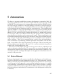
1 Introduction
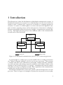
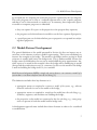
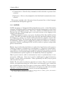
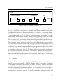
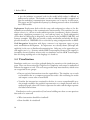
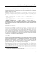
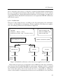
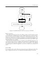
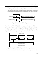
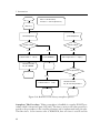
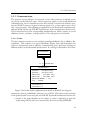
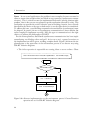
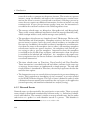
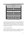
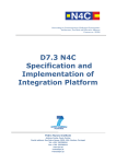
This dissertation is about the development of distributed communication systems. A
distributed communication system is a set of distributed processes that interact with one
another to meet a common goal. A process is an instance of a computer program in
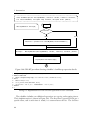
execution. It consists of a timed sequence of actions and events that depend on computer resources, operating system, and on other processes. Interaction is realized via
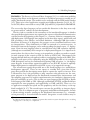
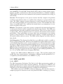
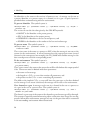
messages transmitted between the processes through a communication network (Figure 1.1). This implies that the processes run at different nodes of the communication
network and are thus distributed.
Node 2
Process 2
Process 1
Process N
Node 1
Node N
Communication Network
virtual link
physical link
Figure 1.1: A distributed communication system as a set of interacting processes.
A good example of a similar type of system would be that of a bridge construction
site. Indeed, all people working at the site can be seen as processes. They perform
a common task, that is the construction of the bridge. During work they communicate with each other and exchange materials needed for work, which is similar to the
exchange of data between processes via messages. Communication between workers
takes place over the air or telephone network. This is equivalent to the communication
network that is used by the processes for interaction.
Distributed communication systems have gained a substantial importance over the
past years. There is a large set of examples of systems that are present in our everyday
1
1 Introduction
life. Examples of such systems are the world wide web (www), peer-to-peer networks,
sensor networks, grid computing, etc. Some of them have applications in different domains, e.g., sensor networks are used in fire detection, weather monitoring, earthquake
early warning, etc. The heterogeneity of applications and application domains speaks
for the complexity of such systems and the challenges that developers are faced with.
This complexity is due also to the existence of two sides of the system that need to be
considered during development:
• the distributed communication infrastructure that includes the nodes (e.g., sensor
nodes), communication medium (e.g., wifi), operating system, communication
protocols, and
• the software applications running on top of the distributed infrastructure and
providing services to the users (e.g., application deciding whether a fire alarm
should be issued or not).
The focus of this dissertation is on the development of applications for distributed
communication systems. There are two aspects that need to be considered during application development. The first and most obvious is the development of the application
itself that will be deployed on the existing distributed communication infrastructure.
The second and less obvious, but equally important, is the analysis of the deployed
application. In simple terms, the purpose of the analysis is to show whether the application is delivering the requested services to the user according to specifications.
This aspect of the development becomes crucial especially when the applications drive
safety-critical systems. An example would be a misbehavior in the application that can
lead to a situation where a fire alarm should be issued but it is not. Such misbehavior
can lead to a life threatening situation and should be avoided by all means.
1.1 Problem Statement
Application development and analysis are like “two sides of the same coin”. An application cannot be deployed successfully unless its analysis confirms that the requirements
are met. On the other hand, an accurate analysis is possible if the application has been
deployed and is running on the intended distributed infrastructure. To solve this deadlock, the common solution is to perform the analysis not on the application but on its
abstraction. This abstraction can be seen as a selection of properties of the application
relevant for analysis.
The separation between application development and analysis increases the cost and
effort required during the development process. There are two factors that contribute
to this increase. First, the method used for deriving the abstraction for analysis differs from that used to develop the application, thus the derivation of an abstraction
becomes a development process of its own. Second, because of the difference in the
2
1.2 Approach
development methods, a thorough validation process is required to ensure that the derived abstraction is an accurate representation of the application, otherwise the results
obtained cannot be used for the analysis.
1.2 Approach
To decrease the development cost and effort, the approach of this dissertation is to
combine and extend existing technologies for obtaining a unified development method.
Unification implies the use of the same development method for both application and
analysis. This calls for a development method that is independent from its final product, be it the application ready for deployment or an abstraction of the later destined
for analysis. The approach consist in capturing the aspects of the application at a higher
level of abstraction. This allows the generation of artifacts that are independent from
the final target, consequently they can be used to drive application development and
analysis. Furthermore, the aim is to automatically derive an application ready to be
deployed on a distributed communication infrastructure and its corresponding abstraction to be used at the same time for analysis.
1.3 Hypothesis
The product of a unified development method is a unified description of the application
that is independent from its final target (i.e., deployment or analysis). In addition, the
description must capture the aspects of the application at sufficient level of detail so
that the final target can be automatically derived. This calls for appropriate description
means and an automated transformation mechanism. In this context, the hypothesis of
this dissertation is that:
The properties of the application can be captured in a unified description which can drive
automatic transformation for deployment on real infrastructures and/or analysis.
1.4 Contributions
The contributions of this dissertation can be summarized as follows:
• an approach for capturing the aspects of an application and producing a unified
description of it,
• an approach for automatically transforming this description into:
– the application itself, to be deployed on the intended distributed communication infrastructure, and
3
1 Introduction
– an accurate simulation model of the application to be used for analyzing its
properties,
• an approach for an in-depth analysis of the system that:
– captures all events during runtime and stores them appropriately, and
– visualizes all captured events to drive analysis.
Furthermore, tool support is provided for each of these approaches, and a real-world
case study is reported for demonstrating their feasibility and the usability of the tools.
1.5 Structure
This dissertation is structured as follows:
• Chapter 2 introduces the terminology that serves as foundation for this work.
• Chapter 3 positions this work in relation to existing state-of-the-art.
• Chapter 4 presents the approach for capturing the aspects of the application and
producing a unified description of it.
• Chapter 5 presents the approach for automatic transformation for deployment
and simulation.
• Chapter 6 presents the approach for visual in-depth analysis of the application.
• Chapter 7 reports the development of an alarming protocol for earthquake early
warning as a real-world case study.
• The dissertation concludes in Chapter 8.
4
2 Background
This dissertation covers the fields of model-driven development, simulation, and visualization of distributed communication systems. A brief introduction of these systems
was given in Chapter 1. This chapter introduces the terminology which serves as the
foundation for this work. At first, a definition for the model and model-driven development is given. These allow capturing of relevant properties of the system in a
unified description. The second part focuses on simulation as the method used in this
dissertation for experimentation and analysis. The chapter concludes by introducing
the concept of visualization.
2.1 What is a Model?
The term model is widely used in several domains. Mathematics, physics, biology,
social science, civil engineering, software engineering, and many more make frequent
use of the term. These domains have their own definition of the model, however, all
definitions can be seen as a more detailed description of the very generic definition:
A model is anything that is (or can be) used, for some purpose, in place of something else [1].
Although very generic, this definition captures all key aspects present in every model
definition. The first aspect is that a model can be anything. This is very true considering
that a model can be:
• a formula representing a law in physics,
• a miniature representation of a bridge in some kind of material,
• code in a programming language representing a computer program, etc.
The second aspect is that the model serves some purpose. Considering the given examples, the purpose of the listed models can be:
• a formula in physics is used for calculations,
• a miniature bridge is used to test resistance in a wind tunnel,
5
2 Background
• code is used by programmers to transform their ideas into computer programs
with the help of compilers, etc.
The last aspect has to do with the model replacing something else. This usually means
that, for the indented purpose, the model is used instead of what it represents:
• a physical law in itself is impossible to use in calculations, thus a formula seems
appropriate,
• it is almost impossible to test the bridge itself for wind resistance, thus a miniature
representation is used,
• it is quite challenging expressing ideas in digital signals (0s and 1s), thus programming languages are used, etc.
Having a general definition of the model, it is time to place it in the context of this
dissertation.
2.1.1 Software Models
Based on the definition given in Chapter 1, a distributed communication system is a set
of interacting processes as part of a computer program in execution. In simple terms,
the system is the computer program in execution on the distributed communication infrastructure. According to the definition of the model, the whole development process
of such systems is based on models. This is true because every computer program is derived from code artifacts. These artifacts are a representation of the computer program
(a model of it), and they are used by the compiler to obtain an executable form (the
computer program itself). In this case the model must capture all properties of what it
represents, i.e., the code describes everything the computer program will do, and the
program will do what the code tells. This tight coupling between the code and the
computer program derived from it often creates the idea that they are the same thing.
This idea is deeply embedded in the terminology used today, i.e., the process of writing
code is called programming (as in building a program) and not modeling (as in building
a model of a program).
Modeling in software development is usually associated with some other description
method that is not code. A typical and very popular example of this is the UML class
diagram [2], which captures the static structure of a program using classes, attributes,
operations, and relations. It is much easier to relate this case to the definition of the
model, because class diagrams capture only static properties (not everything like the
code does) and they are used for better understanding this static structure (not for generating the program through a compiler). Of course they can be used to generate code,
but it will not be complete and thus not enough for generating the final executable.
Nevertheless, this code can suffice for generating another computer program that can
6
2.2 Model-Driven Development
be executed just for analyzing the structural properties captured by the class diagram.
This other program can be seen as a reduced representation of the complete program,
and thus it can be characterized as a model of it. In summary, three important aspects
of models of computer programs are identified:
• they can capture all or part of the properties of the program they represent,
• the program can be derived from its model in case the later captures all properties,
• a partial program can be derived when part of properties are captured for analyzing those properties.
2.2 Model-Driven Development
The general definition of the model presented in Section 2.1 does not impose any restrictions on the existence of what a model is representing. This is true considering for
instance the example of the bridge. The model of the bridge used for testing its wind
resistance is usually built before the bridge itself. This is understandable because the
bridge cannot be build unless the tests on its model fulfill the safety requirements. Another aspect to be noted in this example is that the bridge will be build using its model
(that passed the wind resistance test) as a reference. In this case the model of the bridge
is used for building the bridge itself. So, in a nutshell:
Model-driven development (MDD) is simply the notion that we can construct a model of a
system that we can then transform into the real thing [3].
This definition includes three key elements in it:
• appropriate means are required to construct a model of the system, e.g., relevant
materials and tools in case of the model of the bridge,
• appropriate means are required to transform the model into the real thing, e.g.,
architects, engineers, and machines for building the bridge,
• the properties of the model are transferred to the the real thing, e.g., safety properties are present in both the model and the bridge itself.
A development approach must include these three elements in order to be considered
as model-driven.
7
2 Background
2.2.1 Model-Driven Software Development
Based on the definition of MDD, any software development approach is in itself modeldriven. This is true because:
• programming languages are the tools used to write code, which represents the
model of a computer program,
• compilers transform the code into the actual computer program, and
• the computer program does what the code tells, meaning that all properties expressed in code are transferred to the program.
If the above statement is true then why introduce the term model-driven software development (MDSD)? The answer to this question can be found in the key elements of
model-driven development listed Section 2.2 and specifically to the appropriate means.
There exist several types of software depending on the application domain. These types
usually differ from one another because the set of properties they need to capture is
strictly connected to the domain. For example, the accounting software used in a bank
does not care about interpreting signals about room temperature or smoke. In the
same way, the fire alarming software in the same bank does not care about the account
balance of a customer. This heterogeneity implies the availability of means to capture
properties from different domains. These means are of course present in most programming languages. That is why they are able to model software for different application
domains and often associated with the term general purpose language (GPL). Although
possible, the development of complex software (e.g., distributed communication systems) using GPLs requires considerable skills and time, which are translated into an
increase in cost and effort.
The goal of MDSD is to increase the level of abstraction in software description so
that its properties are captured in a way that is closer to the application domain and thus
decreasing cost and effort required in the process. This is realized with the introduction
of software modeling languages (e.g., UML) and transformation technologies. In MDSD
the modeling language is used to capture the properties and produce a software model
which is transformed into code ready to be compiled for obtaining its executable form
(the computer program). An important concept introduced here is transformation or
simply code generation. In principle there are two approaches to code generation:
• The code is generated manually using the model as a reference. If this approach
is adopted then the focus of the development will be the code and not the model.
This will shift the development process towards model-based, where the models,
although important, do not drive the process itself. Due to this shift there is a risk
for the models to be used only for documentation purposes. Also, inconsistencies
between the model and the code are not rare.
8
2.3 Simulation
• The code is generated automatically. This implies the existence of computer program (the code generator) that can transform the model into code. Furthermore,
the generated code must not require further manual modification, but it should
be ready for compilation.
Automation is the heart of pragmatic MDSD [4]. Also, it is important for MDSD to
be able to take advantage of legacy code libraries and other legacy software [4]. This
is crucial for complex software like distributed communication systems, where the application cannot provide its service without interacting with the underlying communication infrastructure. This requires a description mechanism that allows integration of
operating system calls or protocol interfaces inside software models. Also, this mechanism must provide means for integrating simulation libraries in case the final product
of the code generator is a computer program destined for analysis through simulation.
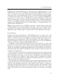
2.3 Simulation
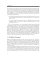
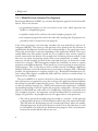
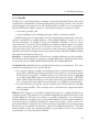
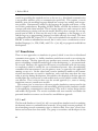
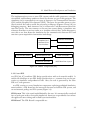
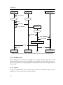
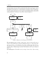
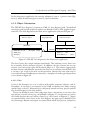
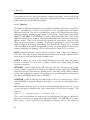
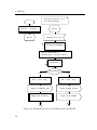
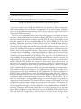
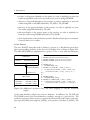
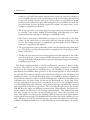
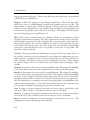
One of the reasons why models exist is experimentation. Experimentation methods can
be classified as shown in Figure 2.1.
System
Experiment with the System
Experiment with a Model of the System
Physical Model
Mathematical Model
Analytic Analysis
Simulation
Figure 2.1: Methods of experimentation for system analysis.
Although not explicitly, the concept of experimentation was introduced already in the
example of the bridge. Recall that the model of the bridge was used to test its wind
resistance. These tests are a series of experiments in a wind tunnel with the purpose of
analyzing those properties of the bridge related to wind resistance. The results of this
analysis can be used to decide whether the safety requirements are met.
Simulation is the imitation of the operation of a system over time, for the purpose of better
understanding and/or improving that system [5, 6].
9
2 Background
Imitation and system are synonyms with model and what the model represents. This
implies a strong relation between models and simulation. That is why the imitation
is usually referred as the simulation model. While models in general can capture any
properties, simulation models lean towards dynamic properties, i.e., those properties
that characterize operation over time. Also, simulation models usually do not capture
all properties but only those relevant to the analysis.
The focus of this dissertation is on computer simulation. In computer simulation the
model is a computer program (in execution). The properties of the bridge that are affected by the wind over time can be also captured by a set of mathematical equations
expressed in program code. The same can be stated for the wind properties that affect
the bridge. These pieces of code can be combined together and then compiled to produce an executable computer program. The purpose of this computer program is the
same with that of the miniature (physical) model of the bridge in the wind tunnel, that
is testing for wind resistance. Computer simulation can be very useful in cases where
construction of a physical model is impossible or cost and effort inefficient. Another
advantage is the ability to easily change or modify captured properties without having
to rebuild the model from scratch, which is not possible with physical models.
2.3.1 Discrete Event Simulation
Simulation models can be classified depending on how time advances during simulation.
Two basic methods of advancing time in simulation are time-stepping and discrete-event.
Time-stepping implies advance in small time increments, where time is represented as
a continuous variable. It is suitable for simulating systems whose properties can be
captured with a set of differential equations. Discrete-event simulations are executed
by processing a series of events and not by directly advancing time. Discrete event
simulation models generate and process events, where each generated event is stamped
with the time at which it needs to be processed. The simulator keeps track all of
pending events (events to be processed) in a data structure called the event list, which
allows the simulation to determine the event to be processed next. The current time
can be viewed as the minimum time-stamp in the event list, that is the time associated
with the first event in the list. Two main approaches can be used for the development
of discrete event simulations:
• The event-oriented approach uses events as its basic modeling construct. Employing an event-oriented approach to model a system is akin to using assembly language to write a computer program: it is very low-level and consequently more
efficient and difficult to use; especially for larger systems.
• The process-oriented approach describes a system as set of interacting processes
and uses a process as the basic modeling construct. A process is used to encapsulate a portion of the system as a sub-model in the same way classes do in an
10
2.4 Visualization
object-oriented programming language. Typically, process-oriented simulation
models are built on top of event-oriented simulators.
2.3.2 Simulation of Software Systems
The process of constructing a simulation model is not trivial. It is simpler to experiment with a physical model, taking for granted that the physical model can be constructed efficiently. For example, the construction of a miniature model of the bridge
will be like that of constructing the bridge itself. On the other hand, constructing a
mathematical model of the bridge is not straightforward because the methodology and
expertise required differs from that required to construct the bridge itself. This change
in methodology requires for the models to be valid, otherwise the results of simulation
will be useless. Computer simulation does require a change in methodology, but there
are cases where it is a better choice. These are the cases where computer simulation is
used for experimentation of software. Indeed, both software and its simulation model
are computer programs in execution. Nevertheless, they are by no means the same
considering that the code used to derive each of them is not the same. So in principle,
to take advantage of this similarity, an abstraction mechanism is required to capture
the properties of the software independently from the final target, i.e., the actual computer program or its model for simulation. This mechanism can be provided by the
model-driven software development paradigm.
2.4 Visualization
According to the definition given in Section 2.3, the purpose of simulation (and experimentation in general) is better understanding and/or improvement. In this context,
experimentation with a physical model is better suited than computer simulation. Indeed, the reaction of a bridge to different wind speeds and directions can be better
understood on a miniature model than with a set of numbers (data) produced by computer simulation. This is due to the change in methodology introduced in Section 2.3.2.
To solve this problem, the data has to be presented somehow in a form closer to the domain. This can be achieved with a recovery mechanism to the change in methodology
so that the results of computer simulation can be presented with something closer to a
physical model. This mechanism can be provided by computer visualization.
Visualization is the use of computer-supported, interactive, visual representations of data to
amplify cognition [7].
In the example of the bridge computer graphics can be used to construct a 3D model
of the bridge. The data resulting from simulation can animate this graphical model to
mimic its behavior on wind conditions.
11
3 Related Work
This chapter introduces state-of-the-art methods and technologies for the development,
simulation, and visualization of distributed communication systems. In the first part
the focus is on modeling languages as the core component of any model-driven approach. The selection of the languages is done based on their capabilities for capturing
the properties of distributed communication systems in a sufficient level of abstraction. The possibility of their usage in a pragmatic model-driven approach is discussed
in terms of technologies and tools. The second part focuses on the simulation of distributed systems. Here the most popular simulation frameworks and/or libraries are
introduced. The third part introduces existing work that uses a model-driven approach
for the development and simulation of distributed communication systems. A discussion is made on whether the presented works provide a complete pragmatic modeldriven approach. The final part is dedicated to related contributions on visualization
of distributed communication systems.
3.1 Modeling Languages
The modeling language is the heart of model-driven development. It provides the necessary abstractions for capturing the properties in form of artifacts. These artifacts
are then used as inputs for an automated mechanism (code generation) that transforms
these descriptions into code to be compiled for obtaining the computer program for
deployment and a simulation model of it for experimentation.
There exist several modeling languages for distributed communication systems. The
focus here is on popular and/or standardized modeling languages. Standardization is an
important aspect because it provides a significant impetus for further progress because
it codifies best practices, enables and encourages reuse, and facilitates inter-working
between complementary tools [4].
The languages are introduced in the following paragraphs by shortly describing their
approach for capturing the properties of distributed communication systems. These
properties are:
• Structure – What are the building blocks (or components) of the system and how
are they organized?
• Behavior – How do these components perform their activities (functional properties)?
13
3 Related Work
• Communication – How do they communicate with each-other to perform their
activities?
• Deployment – How are they deployed on the distributed communication infrastructure?
This section concludes with a discussion about the potential use of these languages
in a model-driven development approach.
3.1.1 LOTOS
LOTOS (Language of Temporal Ordering Specification) [8] is a formal description
technique1 developed within ISO (International Standards Organization) for the formal
specification of distributed systems. There exist a number of LOTOS tutorials in the
literature [10, 11]. This paragraph gives a very brief overview of the language in the
context of the dissertation.
LOTOS specifications consist of two parts: the Abstract Data Types (ADT) and the
Control. The ADT part defines the data types and value expressions needed to specify
the behavior of a system. It is based on the formal theory of algebraic abstract data
types ACT-ONE [12]. The Control part describes the internal behavior of the system.
It is defined by a behavior expression followed by possible process definitions. A behavior
expression is built by combining LOTOS actions by means of operators and possibly
process’ instantiations.
Process A process describes the behavior of a physical or logical entity in the system or
a function. It appears as a black-box to its environment, i.e., the process’ internal behavior is hidden to the environment. The encapsulation provided by the process concept
makes this part of the language highly suitable for specifying communicating objects in
a telecommunication system. A process is also defined by a behavior expression.
Gate A process interacts with its environment by means of synchronization at common points called gates. Gates may be used to model logical or physical interfaces
between a system and its environment. Values, specified by the ADT, may be passed
and received at these gates.
Action The basic units in a behavior expression are actions. They are atomic, instantaneous, and synchronous behaviors. Each action is associated with a gate, namely the
gate at which the event occurs. Two types of actions exist in LOTOS. There are actions
that need to synchronize with the environment of the process in order to be executed;
and there are internal actions, that a process can execute independently.
1A
formal description is a description expressed in a language whose vocabulary, syntax, and semantics
are formally defined (mathematically sound) [9].
14
3.1 Modeling Languages
3.1.2 Estelle
Estelle [13] is a formal description technique, also developed within ISO, for the formal
specification of distributed, concurrent information processing systems. An overview
of the language is also given in [14, 15]. Estelle may be viewed as a set of extensions to
ISO Pascal [16] that model a system as a hierarchical structure of automata which:
• may run in parallel, and
• may communicate by exchanging messages and/or by sharing variables.
A distributed system is composed of several communicating components; each component is specified by a module definition. The module definition consists in a set of
actions (transitions). A module is active if its definition includes at least one transition; otherwise, it is inactive. Each module has a number of input/output access points
called interaction points, which can be external or internal. A channel is associated to
each interaction point. Interactions are abstract events (messages) exchanged with the
module environment (through external interaction points) and with children modules
(through internal interaction points).
Structure A module definition in Estelle may include definitions of other modules.
This leads to a hierarchical tree structure of module definitions. Estelle provides means
to create instances of child modules defined within the module definition.
Communication Module instances within the hierarchy can communicate. Two communication mechanisms can be used in Estelle:
• In a message exchange a module can send interactions to another module through a
previously established communication link between their two interaction points.
An interaction received by a module instance at its interaction point is appended
to an unbounded FIFO queue associated with this interaction point. The FIFO
queue either exclusively belongs to the single interaction point (individual queue)
or it is shared with some other interaction points of a module (common queue).
• In restricted sharing of variables certain variables can be shared between a module
and its parent module. These variables have to be declared as exported variables
by the module.
Behavior The behavior of a module is expressed in terms of a nondeterministic state
transition system. The initial state of a module is defined in the initialization part of the
module definition. The next-state-relation of a module is defined by a set of transitions
declared within the transition part of the module definition. Each transition definition
contains necessary conditions enabling the transition execution, and an action to be
performed when it is executed. An action may change the module state and may output
interactions to the module environment. Actions are defined using Pascal. The well
known model of finite state automaton (FSA) is a particular case of a state transition
system, hence it may be described in Estelle.
15
3 Related Work
3.1.3 UML
UML (Unified Modeling Language) [2] is a general-purpose visual modeling language
standardized by OMG (Object Management Group). It is used to specify, visualize,
construct, and document the artifacts of a software system. It is intended for use with
all development methods, life-cycle stages, application domains, and media. UML includes semantic concepts, notation, and guidelines. It has static, dynamic, environmental, and organizational parts. The UML specification [2] does not define a standard
process but is intended to be useful with an iterative development process.
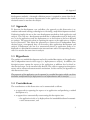
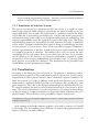
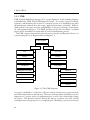
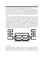
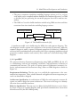
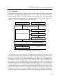
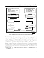
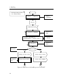
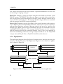
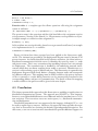
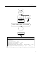
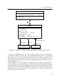
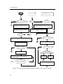
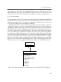
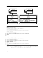
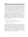
The UML captures information about the static structure and dynamic behavior of
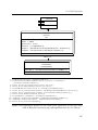
a system using the set of diagrams shown in Figure 3.1.
UML Diagram
Structure
Behavior
Class
Use Case
Object
Activity
Package
State Machine
Component
Interaction
Composite Structure
Sequence
Deployment
Communication
Profile
Interaction Overview
Timing
Figure 3.1: The UML diagrams.
A system is modeled as a collection of discrete objects that interact to perform work
that ultimately benefits an outside user. The static structure defines the kinds of objects
important to a system and to its implementation, as well as the relationships among
the objects. The dynamic behavior defines the history of objects over time and the
communications among objects to accomplish goals. Modeling a system from several
16
3.1 Modeling Languages
separate but related viewpoints permits it to be understood for different purposes.
Structure Diagrams Structure diagrams show the static structure of the system, its
parts, and their relations on different abstraction levels. The elements in a structure
diagram represent the meaningful concepts of a system, and may include abstract, real
world, and implementation concepts. Structure diagrams do not use time related concepts, i.e., do not show the details of dynamic behavior.
• The class diagram describes the structure of a system by showing the system’s
classes, their attributes, and the relationships among the classes.
• The object diagram shows a complete or partial view of the structure of a modeled
system at a specific time.
• The package diagram describes how a system is split up into logical groupings
(packages) by showing the dependencies among these groupings.
• The component diagram describes how a software system is split up into components and shows the dependencies among these components.
• The composite structure diagram describes the internal structure of a class and the
collaborations that this structure makes possible.
• The deployment diagram describes the hardware used in system implementations
and the execution environments and artifacts deployed on the hardware.
• The profile diagram is an auxiliary diagram which allows defining custom stereotypes, tagged values, and constraints. It has been defined in for providing a lightweight extension mechanism to the UML standard.
Behavior Diagrams Behavior diagrams show the dynamic behavior of the objects in a
system, which can be described as a series of changes to the system over time.
• The use case diagram describes the functionality provided by a system in terms of
actors, their goals represented as use cases, and any dependencies among those use
cases.
• The activity diagram describes the business and operational step-by-step workflows of components in a system.
• The state machine diagram is used for modeling discrete behavior through finite
state transitions.
• The interaction diagrams, a subset of behavior diagrams, emphasize the flow of
control and data among the things in the system being modeled:
– The sequence diagram shows how objects communicate with one another in
terms of a sequence of messages. It also indicates the lifespans of objects
relative to those messages.
17
3 Related Work
– The communication diagram shows the interactions between objects or parts
in terms of sequenced messages. They represent a combination of information taken from class, sequence, and use case diagrams describing both the
static structure and dynamic behavior of a system.
– The interaction overview diagram provides an overview in which the nodes
represent communication diagrams.
– The timing diagrams is a specific type of interaction diagram where the focus
is on timing constraints.
3.1.4 SDL
SDL (Specification and Description Language) [17] is a formal description technique
developed by ITU-T (International Telecommunication Union - Telecommunication
Standardization Sector) for the formal specification and description2 of telecommunication systems. The language is used in the development of advanced technical systems,
e.g., real-time systems, distributed systems, and generic event-driven systems where
parallel activities and communication are involved. Typical application areas are highand low-level telecommunication systems, aerospace systems, and distributed or highly
complex mission-critical systems.
A basic model of a system in SDL consists of a set of extended finite state machines
(FSMs) that run in parallel. These machines are independent of each other and communicate with discrete signals.
Structure SDL comprises four main hierarchical levels: system, blocks, processes, and
procedures. Each SDL process is defined as a nested hierarchical state machine. Each
sub state machine is implemented in a procedure. Procedures can be recursive; they
are local to a process or they can be globally available depending on their scope. SDL
also supports the remote procedure paradigm, which allows one to make a procedure
call that executes in the context of another process. A set of processes can be logically
grouped into a block (subsystem). Blocks can be nested inside each other to recursively
break down a system into smaller and maintainable encapsulated subsystems.
Communication SDL does not use any global data. SDL has two basic communication mechanisms: asynchronous signals (and optional signal parameters) and synchronous remote procedure calls. Both mechanisms can carry parameters to interchange and synchronize information between SDL processes and with an SDL system
and its environment (e.g., non-SDL applications or other SDL systems). SDL defines
clear interfaces between blocks and processes by means of a combined channel and signal route architecture. SDL defines time and timers in a clever and abstract manner.
2 According
to [17]: a specification of a system is the description of its required behavior; and a description of a system is the description of its actual behavior, that is, its implementation.
18
3.1 Modeling Languages
Time is an important aspect in all real-time systems but also in distributed systems. A
SDL process can set timers that expire within certain time periods to implement timeouts when exceptions occur but also to measure and control response times from other
processes and systems. When a SDL timer expires, the process that started the timer
receives a notification (signal) in the same way as it receives any other signal. Actually
an expired timer is treated in exactly the same way as a signal. SDL time is abstract
in the sense that it can be efficiently mapped to the time of the target system, be it an
operating system timer or hardware timer.
Behavior The dynamic behavior in a SDL system is described in the processes. The
system/block hierarchy is only a static description of the system structure. Processes
in SDL can be created at system start or created and terminated at run time. More than
one instance of a process can exist. Each instance has a unique process identifier (PID).
This makes it possible to send signals to individual instances of a process.
Data SDL accepts two ways of describing data, abstract data type (ADT) and ASN.1
[18]. The integration of ASN.1 enables sharing of data between languages as well as
reusing existing data structures. The ADT concept used within SDL is very well suited
to a specification language. An abstract data type is a data type with no specified data
structure. Instead, it specifies a set of values, a set of operations allowed, and a set of
equations that the operations must fulfill. This approach makes it simple to map an
SDL data type to data types used in other high-level languages.
3.1.4.1 SDL UML Profile
The SDL UML Profile [19] allows transition from the more abstract UML models
to the unambiguous SDL models. A SDL model can be treated as a specialization of
the generic UML model thus giving more specific meaning to entities in the application domain (e.g., blocks, processes, channels, etc.). A number of features have been
introduced in SDL which directly support SDL and UML convergence:
• UML-style class symbols provide both partial type specifications and references
to type diagrams containing the definition of that type;
• UML-style graphics for SDL concepts such as types, packages, inheritance, and
dependencies;
• composite states that combine the hierarchical organization of state machine diagrams with the transition-oriented view of SDL finite state machines;
• interfaces that define the encapsulation boundary of active objects; and
• associations between class symbols.
19
3 Related Work
While UML has its focus and strength on object oriented data modeling, SDL has its
strength in the modeling of concurrent active objects, of the hierarchical structure of
active objects, and of their connection by means of well-defined interfaces.
3.1.4.2 SDL-RT
SDL-RT (Specification and Description Language - Real Time) [20] is based on the SDL
standard extended with real time concepts. It introduces support of UML in order to
extend SDL-RT usage to static parts of the embedded software and distributed systems.
SDL-RT builds on the fact that SDL is not suited for any type of coding. Some parts
of the application still need to be written in C, C++, or other programming languages.
Furthermore, legacy code or off the shelf libraries such as operating systems, protocol
stacks, and drivers have C/C++ programming interfaces. Last but not least, there
are no SDL compilers so SDL needs to be translated into C code to get down to the
target. So all SDL benefits are lost when it comes to real coding and integration with
real hardware and software. Considering these limitations, SDL-RT provides real time
extension to SDL based on two basic principles:
• replace SDL data types by C/C++ data types and
• add semaphore support.
Also, UML diagrams have been added to SDL-RT to extend its application field:
• The class diagram brings a perfect graphical representation of the classes’ organization and relations. Dynamic classes represent SDL agents and static classes
represent C++ classes.
• The deployment diagram is used to describe distributed systems. It offers a graphical representation of the physical architecture and how the different nodes communicate with each other.
3.1.5 Outlook
In addition to the modeling languages listed above, there exist a number of other languages that are used in research and/or industry. Relevant languages are:
CPN Colored Petri Nets [21] is a language for modeling and validation of concurrent
and distributed systems and other systems in which concurrency, synchronization, and
communication plays a major role. The CPN modeling language is supported by the
computer tool CPN Tools [22]. CPN are quite popular and find use in several applications [23, 24, 25, 26, 27, 28]. CPN have been used also for the verification of UML
[29, 30] and SDL [31, 32] models.
20
3.1 Modeling Languages
PROMELA The Process or Protocol Meta Language [33] is a verification modeling
language that allows for the dynamic creation of concurrent processes to model, for example, distributed systems. The models can be analyzed with the SPIN model checker
[33]. There exist several application examples from different domains [34, 35, 36, 37].
As in CPN, efforts were made to verify UML [38] and SDL [39] models in PROMELA.
The reason why these languages are left outside this discussion is that they focus only
on system analysis3 and not on their development.
The first issue to consider in the assessment of the introduced languages is whether
they provide description means for capturing the aspects of distributed communication
systems listed at the beginning of this chapter, i.e., structure, behavior, communication,
and deployment. All languages have support for the first three aspects, with Estelle and
SDL providing a clear, distinct, and formal definition. Although UML does make a
distinction by means of its diagrams, the concepts are not formalized and leave room
for interpretation. These deficiencies of UML are referred as its variation points. A
distinction between the languages can be made regarding the fourth aspect, i.e., deployment. From the four languages taken in consideration only UML mentions explicitly
(although not formalized) such concept in its deployment diagram. It is important to
mention here also the fact that, because of its popularity, an effort was made to formalize such concepts in the context of SDL by means of eODL [40]. Unfortunately the
language did not find any real application due to overlapping concepts with UML. Nevertheless, such aspect can be captured by using the UML-SDL profile as it is actually an
UML description and can be combined with existing UML notations, i.e., the deployment diagram. A more direct approach would be to use SDL-RT, because it explicitly
defines deployment in combination with SDL as part of its supported concepts.
The second issue regards the possible use of the listed languages in a model-driven
development approach. There are two aspects to consider here, given that the language does provide the description means used to capture the aspects of interest. First
is automation, that is the possibility to fully automate code generation for the computer program to be deployed on the distributed communication infrastructure and
the computer program to be used for experimentation via simulation. Automation implies the availability of tools.4 This is what sets apart languages like LOTOS or Estelle
with languages like UML or SDL. Although standardized, LOTOS and Estelle did not
experience the same popularity and applicability of UML and SDL. There are a lot
of application examples that speak for this popularity and also the history of the updated standards [2, 17]. The second aspect concerns the possibility to integrate legacy
software. This is an important part of pragmatic model-driven development, because
it allows existing software running on the distributed infrastructure (e.g., communication protocols) to be used within the model. Integration of such software may be
3 The
focus in on verification and validation.
here is used as short for computer programs that transform system descriptions in a modeling
language into code ready for compilation.
4 Tool
21
3 Related Work
crucial for providing the required services to the user (e.g., distributed communication
is not possible without access to communication protocols). This requires a certain
flexibility from the modeling language defined into concepts for making such integration possible. Unfortunately neither of the languages do provide such means, at least
not in their standard form. Regarding LOTOS, Estelle, and SDL the inclusion of such
concepts will make them informal. This is because support for such concepts in itself
means inclusion of existing code into the model. However, these concepts are not supported even in UML. A reason for this may be the complexity of the language as it is
and the large set of programming languages in which code may be written. This issue
is addressed in SDL-RT, where C/C++ code can be included in the model. Of course,
SDL-RT is neither standardized nor formal, but it can be seen as a combination of standardized languages (i.e., SDL, UML, and C/C++ [41, 42]) for pragmatic model-driven
development.
3.2 Simulation
There are two approaches to simulation in general, which is true also for distributed
communication systems, i.e., build a simulation model from scratch or use existing simulation software. The first approach may produce more accurate results as the whole
process of building a simulation model is part of the development, i.e., no external models are used. However, this approach will become soon unfeasible with the increasing
of complexity, which is actually the case of distributed systems. Also, the underlying
communication infrastructure is not the primary focus, as opposed to the application
running on top of it. On the other hand, accurate simulation models of the communication infrastructure are crucial to simulation, and as such they must have the same
order of priority during development. Nevertheless, the adoption of the first approach
would require the construction of such models from scratch, which is neither time nor
cost effective. That is why in these cases the second approach (i.e., reuse of existing
simulation software) sounds more feasible.
This section gives an overview of the most popular simulation software used in the
field of computer communication and networking which provide simulation models
of the underlying communication infrastructure. The focus is on key design choices
and models they provide. The section concludes with some remarks on whether the
presented simulation software can be used in a model-driven approach.
3.2.1 ns-2
The Network Simulator 2 (ns-2) [43, 44] is an event-driven simulation tool for studying
the dynamic nature of communication networks. It has gained constant popularity in
the networking research community since its birth in 1989. Ever since, several revolutions and revisions have been made. The group of researchers and developers in the
22
3.2 Simulation
community are constantly working to keep ns-2 strong and versatile.
Two languages are used in ns-2: OTcl [45] and C++. The reason behind this choice
was to make writing simulation scripts easy and flexible in Tcl, while implementing the
performance critical code in C++. Tcl is an interpreted language, thus changes to a
simulation script do not require any recompilation. However, this flexibility comes at
the cost of slower execution speed. Also, due to this dual language design, all objects
need to be available in both languages and must provide dual interfaces in C++ and
OTcl.
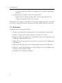
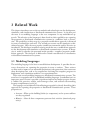
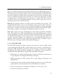
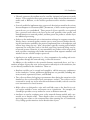
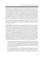
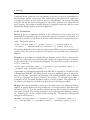
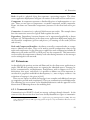
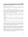
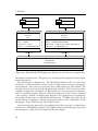
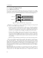
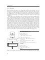
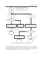
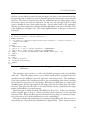
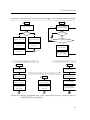
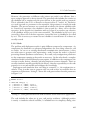
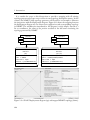
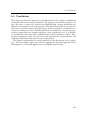
Figure 3.2 shows a generic simulation model in ns-2. The node is the basic component
and serves as a communication endpoint where other components may be attached
to. The link represents the communication medium that connects nodes and can be
one-way or two-way. Every packet that needs to be transmitted over the link is first
inserted into its queue, and when the link is ready to handle it, it is removed from the
queue and delivered to the destination after some delay. Queues and delays are available
for both communication ways when the link is duplex. After the underlying physical
infrastructure has been set (i.e., the nodes and links), the next step would be to define
the protocols so that communication can be possible. Protocols in ns-2 are represented
by agents attached to nodes. The infrastructure is now ready to be used by applications
(also known as traffic generators) for communication. Applications are attached to
agents and use the protocols to communicate with each other.
Application
Application
Agent
Agent
Link
Queue
Delay
Node
Node
Delay
Queue
Figure 3.2: The basic simulation model in ns-2.
3.2.2 ns-3
The Network Simulator 3 (ns-3) [46, 47] is a discrete-event network simulator targeted
primarily for research and educational use. One of the fundamental goals in the ns-3
design was to improve the realism of the models, i.e., to make the models closer in
implementation to the actual software implementations that they represent. Different
23
3 Related Work
simulation tools have taken different approaches to modeling, including the use of specific modeling languages, code generation tools, and component-based programming
paradigms. While high-level modeling languages and simulation-specific programming
paradigms have certain advantages, modeling actual implementations is not typically
one of their strengths. In the authors’ experience [47], the higher level of abstraction
can cause simulation results to diverge too much from experimental results, and therefore an emphasis was placed on realism. For example, ns-3 chose C++ as the programming language because it facilitated the inclusion of C-based implementation code. The
ns-3 architecture is also similar to Linux computers, with internal interfaces (network
to device driver) and application interfaces (sockets) that map well to how computers
are built today. ns-3 is not a new simulator but a synthesis of several predecessor tools,
including ns-2, GTNetS [48], and YANS [49]. A third emphasis has been on ease of
debugging and better alignment with current languages. Architecturally, this led the
ns-3 team away from the mixture of OTcl and C++ which was hard to debug. Instead,
the design chosen was to emphasize purely C++-based models for performance and
ease of debugging, and to provide a Python-based scripting interface.
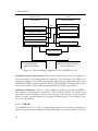
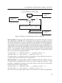
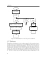
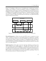
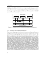
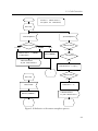
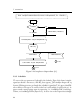
As shown in Figure 3.3, the ns-3 simulator has models for all the various elements of
a computer network.
Node
Node
Application
Application
Socket-like API
Protocol
Stack
Protocol
Stack
Device
Device
Channel
Packet
Figure 3.3: The basic simulation model in ns-3.
• Nodes represent both end-systems such as desktop computers and laptops, as well
as network routers, hubs, and switches.
• Devices represent the physical device that connects a node to a communication
channel. This might be a simple Ethernet network interface card, or a more
complex wireless IEEE 802.11 device.
24
3.2 Simulation
• Channels represent the medium used to send the information between network
devices. These might be fiber-optic point-to-point links, shared broadcast-based
media such as Ethernet, or the wireless spectrum used for wireless communications.
• Protocols model the implementation of protocol descriptions found in the various
Internet Request for Comments (RFC) documents, as well as newer experimental
protocols not yet standardized. These protocol objects typically are organized
into a protocol stack where each layer in the stack performs some specific and
limited function on network packets, and then passes the packet to another layer
for additional processing.
• Packets are the fundamental unit of information exchange in computer networks.
Nearly always a network packet contains one or more protocol headers describing the information needed by the protocol implementation at the endpoints and
various hops along the way. Also, the packets typically contain payload which
represents the actual data (such as the web page being retrieved) being sent between end systems. However, it is not uncommon for packets to have no payload,
such as packets containing only header information about sequence numbers and
window sizes for reliable transport protocols.
• Applications are traffic generators, i.e., they communicate by sending and receiving packets through the network using a socket-like interface.
In addition to the models for the network elements mentioned above, ns-3 has a
number of helper objects that assist in the execution and analysis of the simulation, but
are not directly modeled in the simulation. These are:
• Random variables can be created and sampled to add the necessary randomness
in the simulation. Various well-known distributions are provided, including uniform, normal, exponential, Pareto, and Weibull.
• Trace objects facilitate the logging of performance data during the execution of the
simulation, that can be used for later performance analysis. Trace objects can be
connected to nearly any of the other network element models, and can create the
trace information in several formats.
• Helper objects are designed to assist with and hide some of the details for various actions needed to create and execute an ns-3 simulation. For example, the
CsmaHelper provides an easy method to create an Ethernet network.
• Attributes are used to configure most of the network element models with a reasonable set of default values. These default values are easily changed either by
specifying new values on the command line when running the ns-3 simulation,
or by calling specific functions in the default value objects.
25
3 Related Work
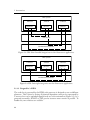
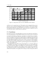
3.2.3 OMNeT++
The Objective Modular Network Testbed in C++ (OMNeT++) [50, 51, 52] is an
extensible, modular, and component-based C++ simulation library and framework. It
has been created with the simulation of communication networks and other distributed
systems in mind as application area, but instead of building a specialized simulator, it
was designed to be as general as possible. OMNeT++ is often quoted as a network
simulator, when in fact it is not. It includes the basic machinery and tools to write
simulations, but itself it does not provide any components specifically for computer
networks, queuing networks, or any other domain. These application areas are supported by various simulation models and frameworks:
• INET Framework [53] is an open-source communication networks simulation
package, which contains models for several Internet protocols: UDP, TCP, SCTP,
IP, IPv6, Ethernet, PPP, IEEE 802.11, MPLS, OSPF, and others.
• INETMANET [54] is a fork of the INET Framework, and extends INET with
support for mobile ad-hoc networks. It supports AODV, DSR, OLSR, DYMO
and other ad-hoc routing protocols.
• OverSim [55] is an overlay and peer-to-peer network simulation framework for
OMNeT++. The simulator contains models for structured (Chord, Kademlia,
and Pastry) and unstructured (GIA) P2P systems and overlay protocols. OverSim
is also based on the INET Framework.
• MiXiM [56] supports wireless and mobile simulations. It provides detailed models of the wireless channel, wireless connectivity, mobility models, models for
obstacles and many communication protocols especially at the MAC level.
• Castalia [57] is a simulator for Wireless Sensor Networks (WSN), Body Area
Networks, and generally networks of low-power embedded devices. Castalia can
be used by researchers and developers to test their distributed algorithms and/or
protocols in a realistic wireless channel and radio model, with a realistic node
behavior especially relating to access of the radio.
The OMNeT++ simulation model is shown in Figure 3.4. It consists of modules
that communicate with message passing. The active modules are named simple modules;
they are implemented in C++ using the simulation class library. Groups of modules
can be encapsulated into compound modules.
In network simulations, simple modules may represent user agents, traffic sources
and sinks, protocol entities, network devices, data structures, or user agents that generate traffic. Network nodes such as hosts and routers are typically compound modules
assembled from simple modules. Both simple and compound modules are instances of
module types. While describing the model, the user defines module types; instances of
26
3.2 Simulation
Network
Compound Module
Connection
Gate
Simple
Module
Figure 3.4: Model structure in OMNeT++.
these module types serve as components for more complex module types. The network to be simulated is an instance of a module type. When a module type is used as
a building block, there is no distinction whether it is a simple or a compound module.
This allows the user to transparently split a module into several simple modules within
a compound module, or do the opposite, re-implement the functionality of a compound module in one simple module, without affecting existing users of the module
type. Modules communicate with messages, which, in addition to predefined attributes
such as a time-stamp, may contain arbitrary data. Simple modules typically send messages via gates, but it is also possible to send them directly to their destination modules.
There are input, output, and inout gates. Gates may be linked with a connection. Due
to the hierarchical structure of the model, messages typically travel through a chain of
connections, to start and arrive in simple modules. Compound modules act as "cardboard boxes" in the model, transparently relaying messages between their inside and the
outside world. Properties such as propagation delay, data rate, and bit error rate can
be assigned to connections. One can also define connection types with specific properties (named channels) and reuse them in several places. Modules can have parameters.
Parameters are mainly used to pass configuration data to simple modules, and to help
define the model topology. Parameters may have default values, units of measurement
and other attributes attached to them.
3.2.4 OPNET
The Optimized Network Engineering Tools (OPNET) [58] is a well-established commercial discrete-event simulator. OPNET Modeler defines a network as a collection
of sub-models representing sub-networks or nodes, therefore it employs hierarchical
modeling. The topology used in a simulation can be manually created, imported or
selected from the pool of predefined topologies. A vast number of protocol models are
available in OPNET Modeler and users can implement their own models. Models are
developed using a four-level structure. Network level handles topology modeling and
27
3 Related Work
overall configuration. Node level deals with internal structures of nodes (transmitters
and receivers), while functional aspects of node level devices are modeled as finite state
machines at the process layer. Proto-C layer, being the lowest layer, is where the coding
of model behavior takes place in Proto-C language which is an extension of C. The
layer contains many kernel procedures, and it allows access to source codes of built-in
models. Nodes are configured by setting their parameters which define their internal
structure as a set of fields or probability density functions. Nodes contain a set of transmission and reception modules, representing a protocol layer or physical resource, to
ensure their connection to communication links. Interactions between modules are
handled by exchanging messages. Users are able to configure applications installed on a
node, and set nodes and links to fail or recover during simulation at specified times. Before simulation execution, one should make a selection of desirable output statistics. It
is possible to specify a set of network simulations and pass a range of input parameters
or traffic scenarios (which can be characterized by models for various applications like
FTP, HTTP, etc.) to them. Statistics about performance of simulated networks can be
collected at runtime.
3.3 Model-Driven Development and Simulation
Due to the popularity and extensive use of their corresponding languages, most existing
model-driven approaches are based on UML and SDL. The purpose of this section is to
give a brief overview of the approaches found in literature. Also an assessment will be
made based on whether they provide support for:
• automatic code generation for each of the aspects of distributed communication
systems for both deployment and simulation, and
• integration with existing legacy software.
This assessment contributes to the motivation of the work presented in this dissertation.
3.3.1 MDD with UML
3.3.1.1 SimML
The Simulation Modeling Language Framework (SimML) [59, 60, 61, 62, 63] is a set of
tools that allow automatic generation of simulation models from UML notations.
The tool-set is shown in Figure 3.5 and consists of:
• The simulation modeling language is a general purpose simulation language that
is used for indeterminate representation of simulation models.
28
3.3 Model-Driven Development and Simulation
• The parser transforms simulation modeling language artifacts to C++ or Java
code, which can be compiled and then linked to the simulation libraries C++SIM
or JavaSim [64] for generating the executable program that will be used for simulation.
• The UML tool is used to build simulation models using UML notations and then
transform them into simulation modeling language artifacts.
UML Design Notation
Simulation Program
SimML Notation
Front-End GUI Tool
Back-End SimML Parser
Figure 3.5: The SimML framework [63].
A simulation model can be build using the UML class and sequence diagrams. The
class diagram is used to capture static properties of the system (its structure), while the
sequence diagram is used to capture its dynamic properties (its behavior). Additional
notations have been defined and can be used by the tool for capturing simulation related
properties (random numbers and statistics) that could not be described using UML
diagrams.
3.3.1.2 proSPEX
The protocol Software Performance Engineering using XMI (proSPEX) [65, 66, 67]
is a methodology and tool for modeling, verification, and performance evaluation of
communication software. The goal is to specify protocol architecture (structure), behavior, and environmental characteristics using a subset of UML diagrams as shown in
Figure 3.6.
Requirements Definition The first step is to establish the requirements of the communication component. Then, suitable network and application inter-component protocols are identified or designed.
Architecture Specification A combination of UML class and composite structure diagrams are used to design the system architecture. The focus of this stage is to identify
the active classes and their interfaces.
Behavior Specification The next step is to define the detailed behavior of active classes
by means of the state machine diagram with specialized communication abstractions
derived from SDL (the SDL-UML profile).
29
3 Related Work
UML Model Editor
proSPEX
UML Model
Simulation Model
Class
XMI
Nodes (an Paths)
Processes
Composite Structure
Workloads
State Machine
Communication
Parameters
Design
Model Execution
Parameter Change
Communication Component
- network protocols
- application protocols
Patterns for Communication
System Architecture
Figure 3.6: The methodology supported by the proSPEX tool [65].
Simulation Scenario Specification The scenario specification starts by modeling of
the environment of the communication component. For this purpose the UML communication diagram is used. Next, performance properties are captured by annotations
embedded in UML comment symbols. Finally, the proSPEX tool imports the specification from which a semantically equivalent simulation model is generated.
Simulation and Results The core of the simulation model generated by proSPEX is
the Simmcast [68] simulation framework. The simulation results are traced events
generated from the simulator: message sent, message read, message arrival in queue,
process creation, process destruction, message discarded, process’ state change, timer
set, reset, and timeout.
3.3.1.3 UML-PSI
The UML-PSI [69, 70, 71, 72] is a methodology and tool for automatic generation of
simulation performance models from high-level UML software descriptions. The first
30
3.3 Model-Driven Development and Simulation
step requires the identification of the performance goals that the system should satisfy.
The next step is the development of a system model in UML; at the same time, UML diagrams are to be annotated with quantitative, performance-oriented information which
will be used to evaluate the software model. Annotations are inserted as stereotypes and
tagged values, according to a subset of the annotations defined in the UML profile for
schedulability, performance, and time specification [73]. The next step is the derivation of the simulation program from the annotated UML diagrams. This step is done
automatically by UML-PSI which parses an XMI [74] representation of the annotated
UML model and builds a process-oriented discrete simulation program for that model
based on a custom C++ simulation library.
Figure 3.7 shows how UML elements are mapped to simulation model elements.
Simulation processes can be divided in three families corresponding to processes representing workloads, resources, and activities respectively. UML actors in use case diagrams are translated into workloads; nodes of the deployment diagrams correspond
to processes that model resources, and action states in activity diagrams are translated
into processes representing the actions. UML annotations are used as parameters for
the simulation model.
UML Model
Simulation Model
Use Case
Workloads
Deployment
Resources
Activity
Activites
Tagged Values
Parameters
Processes
Simulation
Parameters
Figure 3.7: Mapping of UML notations to a simulation model with UML-PSI [71].
3.3.1.4 Syntony
The simulation framework Syntony [75, 76, 77, 78] enables the automated and statistically sound simulation and testing of UML-based models. The well-known modeling standard UML is used to specify a system as well as a test model. The model
is then annotated with quantitative elements and performance metrics using the standardized UML Profile for Modeling and Analysis of Real-Time and Embedded Sys-
31
3 Related Work
tems (MARTE) [79] and UML Testing Profile (UTP) [80] for testing relevant aspects.
Syntony provides a mechanism for the automated translation of standard compliant
UML models into discrete event simulations and systematic mechanisms for testing of
such models.
Structure The description of the system structure basically comprises the problem
of which system elements there are, and how these elements are connected with each
other. The UML composite structure diagrams are used to describe the system structure. These diagrams display the internal structure of classes. This includes how other
classes are nested inside a class, and how the nested classes can communicate via connectors attached to their ports.
Behavior The behavior of the entire system is composed of the functional operation
of each system element and the communication between the elements. The UML state
machine diagrams are used to model the system behavior. There are two levels of detail
to choose from. The less detailed variant is to annotate all transitions with transition
probabilities. These probabilities can come either from measurements of an existing
system or from estimations. The detailed variant requires a complete specification of
all transition effects and state actions. The UML activity diagrams are used to describe
these details.
Code Integration The elements described above are sufficiently suitable to model arbitrary systems and networks. However, this would become quite cumbersome as soon
as the modeled algorithms reach a certain complexity. It is therefore desirable to allow
the usage of code in a textual programming language at least at certain places in a model.
Appropriate UML elements for this are easily identified: OpaqueActions and OpaqueBehaviors allow the specification of a textual body and a corresponding language. Two
different languages are supported: the native language of the underlying simulation core
(i.e., C++), and the Object Action Language (OAL) [81].
Syntony uses UML models in XMI format as input. The tool then analyzes the
model, does some transformations, and outputs a simulation model specified in C++
as required by the used simulation core OMNeT++ [51].
3.3.2 MDD with SDL
3.3.2.1 SPEET
The SDL Performance Evaluation Tool [82, 83, 84] allows performance analysis of
formally specified systems under real-time conditions. The objective of SPEET is the
design and evaluation of complex and formally specified communication systems in an
early phase of their development by means of simulation and emulation.
The modular structure of SPEET is shown in Figure 3.8. The run time system is a
computer program in execution on the same platform SPEET is running (e.g., Linux).
32
3.3 Model-Driven Development and Simulation
The implementation of one or more SDL systems and the traffic generators, transmission models, and hardware emulators chosen by the user are part of this program. The
simulation can be controlled via two types of interfaces: the Command Line Interface
(CLI) and the Graphical User Interface (GUI). The latter also provides means to visualize statistical data and to enable the processing of Message Sequence Charts [85] for
debugging purposes. Both interfaces can be connected to and disconnected from the
run time system. The user connects to the run time system during a simulation run
whenever he wishes to retrieve results or to visualize statistical data, and he disconnects
after this to not slow down the simulation by the communication between GUI and
run time system required for information interchange.
Statistical Evaluation
Graphical and
Command Line
User Interface
Transmission Models
MSC Diagrams
Specification in SDL
Traffic Generators
Hardware Emulator
SPEET Run-Time System
Figure 3.8: SPEET components [84].
3.3.2.2 ns+SDL
ns+SDL [86, 87] combines SDL design specifications with ns-2 network models. It
enables the developer to use SDL design specifications as a common base for the generation of simulation and production code. Also, the code is generated by the same
SDL-to-C code generator.
ns+SDL consists of several simulation components replacing predefined simulation
functionalities, a SDL kernel for the interaction between ns-2 and the SDL system, and
an environment package for SDL systems (Figure 3.9).
SDL System This is the actual model defined by the user. It is automatically translated
into an ns-2 agent ready to be used in simulation. Interfaces are provided in cases where
the application uses routing and/or link layer functionalities.
SDL Kernel The SDL Kernel is responsible for:
33
3 Related Work
SDL Module
SDL System
SDL Environment Interface
SDL Kernel
named
pipe
ns-2 Simulator
Figure 3.9: ns+SDL components [86].
• Dispatching SDL transitions: the SDL Kernel triggers the transition scheduler and
dispatches scheduled transitions.
• Handling of messages between different SDL systems: message exchange between
different SDL systems is controlled by ns-2. The SDL Kernel provides encoding
and decoding functions for the messages.
• Handling of control messages: control messages are exchanged between ns-2 and
the SDL kernel to query the system time or to return control to ns-2 after all
pending transitions have been executed.
• Time synchronization between ns-2 and the SDL system: to support a global
time, the time of ns-2 is synchronized with the time of all SDL systems under
simulation.
Simulation runs can be made reproducible if concurrent behavior is avoided. This is
achieved by two measures. First, the tight synchronization between ns-2 and the SDL
kernel ensures that only one SDL system is executed at any point in time. Second, the
ns-2 scheduler ensures that transitions that are fireable at the same simulation instant
are executed sequentially.
SDL Environment Interface To implement open SDL systems (systems interacting
with their environment), an environment interface satisfying the semantics of the SDL
signaling mechanism is needed. The SDL Environment Interface allows SDL signals to
be exchanged between open SDL systems via a network configured from ns-2 components. It can be configured to interface either to ns-2 or to physical hardware. This has
the advantage that code for simulation and production purposes can be automatically
generated from the same SDL specification with the same code generator.
34
3.3 Model-Driven Development and Simulation
3.3.2.3 WISENES
The Wireless Sensor Network Simulator [88, 89, 90] framework allows rapid design,
simulation, evaluation, and implementation of both single nodes and large Wireless
Sensor Networks (WSN). New WSN design starts from high level SDL model which
is simulated and implemented on a prototype through code generation. Figure 3.10
shows an overview of the WSN design with WISENES.
XML Configuration Files
SDL Model
WISENES Framework in SDL
Sensor Node
Central Simulation Control
Sensing Channel
Transmission Medium
Environment Functions
Socket Interface
Simulator
Figure 3.10: WISENES components [88].
The designer creates protocol layers and applications in SDL. A simulator is automatically generated for the evaluation of a single node and the network of nodes. Code
generation is also used for the final executable for each node. The nodes are parameterized very accurately in eXtensible Markup Language (XML) [91]. A unique feature
in WISENES is the back-annotation of measured results from a physical prototype to
the simulator. In this way WISENES combines the high abstraction level design and
the accurate node performance evaluation into a single framework. The basic steps in
the flow are the creation of a SDL model, functional simulations, the implementation
of a limited scale prototype network, the back-annotation of the performance measurements for SDL model consistency checking and for improving simulator accuracy, and
simulations for a large scale network. Finally, the production ready WSN implementation is obtained. It is also possible to perform only simulations and based on that give
35
3 Related Work
constraints for the platform. This is useful when no physical platform is available or it
is being designed.
3.3.2.4 HUB Transcompiler
The HUB Transcompiler [92, 93] is able to generate C++ code artifacts from SDLRT.5 These different artifacts can be linked after their compilation with different libraries. This allows the construction of different computer programs for deployment
on OpenWrt [95] and simulation with ODEMx [96]. SDL-RT blocks are mapped to
C++ classes that are populated with other blocks or processes, and processes become
C++ classes that have procedures as their methods. To allow sending of messages
among different processes, all processes derive from a common base class. Figure 3.11
gives a generic view on the transcompiler.
SDL-RT Model
RTDS C Macros and Templates
RTDS Code Generator
C Code
HUB Transcompiter
HUB Transcompiler Code Templates
C++ Code
C++ Compiler / Linker
Platform Source Files and Libraries
Executable
Figure 3.11: HUB Transcompiler code generation.
3.3.3 Outlook
In addition to the methodologies and tools already presented, there exist a number of
other approaches for model-driven development and simulation based on UML and
SDL. The reason why they are not described in detail is that they are quite similar to
the ones already introduced. Further information on these approaches can be found in
[97, 98, 99, 100, 101, 102].
Structure and Behavior The introduced methodologies and tools provide means for
capturing structure and behavior properties in different ways. The next step is to investigate whether the captured properties are used as inputs in an automated process
(e.g., code generation) for generating a computer program to be deployed on a real
5 The
36
transcompiler transforms C code generated from RTDS [94] to C++ code.
3.3 Model-Driven Development and Simulation
infrastructure and, at the same time, a simulation model of the later to be used for
experimentation. All UML-based solutions focus only on simulation and there is no
mentioning whether the model is used to automatically generate the real system (i.e.,
computer program to be deployed). The key aspect here is automation in the context
of the same methodology and/or tool. In principle it may be possible to generate the
real system using other automation tools, but these may interpret the model in ways
that may differ from the original approach. This lack of full support for model-driven
development and simulation can be attributed to the limitations of existing tools that
these approaches are based on. On the other hand, the solution provided by SDL-based
approaches is more complete. All of them support automatic generation for both targets, i.e., the computer program to be deployed and its simulation model. However, it
is worth mentioning that this support comes from the existing tools they use, because
their focus is also on simulation. The HUB Transcompiler is an exception because it
adapts the code generated by the tool for either the computer program to be deployed
or its simulation model.
Communication There are two types of communication that need to captured during
modeling: local and distributed. Local communication refers to the communication
between system components running on the same node, while distributed communication refers to the communication between system components running on different
nodes. The later implies the utilization of the underlying communication infrastructure of the distributed system, e.g., operating system, communication protocols, etc.
It is important to make a distinction between the two types of communication, because they are implemented using different communication mechanisms, e.g., shared
memory for local and sockets for distributed. Automatic code generation is possible
only if such a distinction is already present in the model at its structure and behavior
descriptions. Local communication does not require any external mechanism and it is
simpler to embed into the model by using the available description means provided by
the modeling language. On the other hand, distributed communication requires additional description means in order to capture aspects that are already implemented in
the underlying communication infrastructure. There are two approaches for this:
• A model in the corresponding language (e.g., UML or SDL) can be derived from
these implementations. This model can be then used for capturing distributed
communication inside the model of the actual system. This approach is adopted
in Syntony, ns+SDL, and WISENES. A formalized application programming interface (API) [103] has also been defined in the context of ns+SDL using a patternbased approach [104, 105].
• The existing implementation of the communication mechanism can be reused as
it is inside the model. This is the approach adopted by the HUB Transcompiler.
However, this is not a property of the approach but rather of the language it is
based on (SDL-RT). It is hard to consider this as an appropriate solution because
37
3 Related Work
it just the inclusion of external code in the model which makes it difficult to
understand or analyze. The benefits are that no additional model is required and
that the underlying communication infrastructure can be used at its full extent.
This aspect was also exploited in Syntony by allowing external code to be included
into UML models.
Deployment Deployment deals with the setup and configuration values of the distributed system running on the communication infrastructure. This translates in a simulation scenario, i.e., the set of nodes and their position (coordinates), devices, channels,
applications, simulation parameters (e.g., start and stop time), etc. Such configuration
can be done in UML using its diagrams as was shown in the proSPEX, UML-PSI, and
Syntony examples. SDL does not provide a similar mechanism and neither do the approaches based on it. WISENES tries to solve this by using configuration files in XML.
Code Integration Integration with legacy software is an important aspect of pragmatic model-driven development. Its importance was already shown (although not
explicitly) in the case of distributed communication. Only two of the approaches provide support for it, i.e., Syntony and the HUB Transcompiler. However, the support is
incomplete because Syntony focuses only on simulation and the HUB Transcompiler
does not bring anything new to the language it is based on.
3.4 Visualization
Simulation results are a set of data gathered during the execution of the simulation program. These are characterized by a high level of complexity and cannot be understood
without the support of tools. The tools may provide many functionalities, which often
are categorized in two groups:
• Extract statistical information from the acquired data. The simplest case of such
tool would be that of a computer program that reads a file containing the results
and outputs a mean value of some kind.
• Visualize the information contained in the data in a more comprehensible way.
An example would be the graphical representation of a simple network with an
undirected graph, where the vertices represent the nodes and the edges represent
the links between them.
Visualization can be a powerful tool, but before building one there are two questions
that need to be answered:
• What information should be visualized?
• How should it be visualized?
38
3.5 Conclusion
The answers depend on the application domain, e.g., the information that needs to be
visualized in the simulation of a bridge differs from that of a sensor network. In the case
of distributed communication systems a hint to the first question was given in proSPEX
[65] which adopts the idea from [106]. This is considered a hint because there is no
explicit mention of visualization. The information gathered during simulation is used
only for statistical purposes. Regarding the second question, the answer depends on the
approach, although several similarities can be found in existing tools. In summary, the
aim is to visualize simulation results, i.e., the properties of the system over time. This
implies the graphical representation of the structure, behavior, communication, and
deployment over time. The existing methodologies and tools found in the literature
fall into two categories based on what they visualize:
Network Visualization The tools focus on the visualization of the underlying communication infrastructure and are known as packet-level visualization tools. They come
as standalone computer programs, e.g., NAM [107], iNSpect [108], NetViz [109], Yavista [110], NetAnim [111], etc., or as part of a simulation framework, e.g., GTNetS,
OMNeT++, OPNET, etc. These tools and methodologies behind them are appropriate for visualization of large-scale systems, i.e., distributed systems running on hundreds or even thousands of nodes. However, the scalability they provide comes at a
price: they cannot visualize behavior properties in sufficient details.
System Visualization These tools are intended for detailed visualization of events.
The focus is on the application, and the captured events correspond to those representing behavioral properties of the system. These are similar to the events identified
in [65, 106]. The tools can be standalone computer programs, e.g., MscTracer [112],
or bundled with system development tools, e.g., RTDS [94], Rational SDL Suite [113],
etc. They are appropriate for detailed visualization of small-scale systems.
To address the limitations of both categories, the approach of this dissertation is
to combine the presented concepts into a single tool-chain for providing scalability
without affecting the required level of detail.
3.5 Conclusion
This chapter introduced existing state-of-the-art methodologies and tools relevant to
this dissertation. These were grouped into modeling languages, simulation frameworks,
model-driven development and simulation-based approaches, and visualization. For
each of these categories an assessment was made to establish at what extent the existing
state-of-the-art provides support for model-driven development and simulation of distributed communication systems. From this assessment it can be concluded that a mix
of standardized languages (e.g., SDL-RT) provides better description means for capturing the aspects of interest. This was also confirmed, despite the identified deficiencies,
39
3 Related Work
by the existing approaches that are based on such language (e.g., the HUB Transcompiler). The presented solutions did not show any preference as to what simulation
framework could be more appropriate for integration within a model-driven approach.
However, the ns-3 simulation framework can provide better and easier integration due
to its design choice for making the models closer in implementation to the actual software that they represent. Regarding visualization, existing work provides two different
and separated approaches of aiding analysis, but they can be combined for exploiting
their advantages.
The aim of this dissertation is not to “reinvent the wheel” but rather to exploit
and build upon existing approaches by identifying and addressing their deficiencies.
For this purpose the SDL-RT modeling language will be used as a basis for defining a
unified model-driven approach. Also, the ns-3 simulation framework will be used for
experimentation, and visualization concepts will be combined into a single solution.
The following chapters describe in detail the approach of this dissertation, starting
with the modeling of the aspects of the system using SDL-RT.
40
4 Modeling
This chapter introduces the approach of this dissertation to modeling. The first part
focuses on SDL-RT as the base modeling language used by the approach. At first an
overview of relevant features of the language is given based on its standard [20] and
categorized by the aspect they help in capturing, e.g., structure, behavior, communication, or deployment. The features will be introduced by means of a simple example,
i.e., a typical client-server application.
The presentation of the language will be then used to identify missing concepts that
are required for capturing in detail the aspects of distributed communication systems.
These issues will be addressed to allow later (Chapter 5) automatic full code generation.
4.1 Specification and Description Language – Real Time
4.1.1 A Client-Server Application
A simple example of a client-server application will be considered to better understand
how SDL-RT can capture the aspects of a system. The general idea is that one or more
clients issue requests to the server. Upon receiving a request from a client, the server
creates a handler and associates it with the client from which it received the request.
The handler is responsible for carrying out some calculation, but for simplicity its duty
will be only to increment a counter variable just for keeping track of handled requests.
After handling a request and incrementing the counter, the handler will send a reply
to its associated client and terminate. A semaphore will be used to guarantee proper
behavior, because the counter variable will be accessible by all handlers. To ensure
proper termination, a limit will be set for the total requests that will be handled. A
common scenario of execution is given in Figure 4.1.1 The client, server, and handler
processes are named pClient, pServer, and pHandler. The client sends mRequests to
the server which creates a handler and sends a mHandle to it with the identifier (not
shown in the figure) of the client. The handler tries to take the semaphore lockCounter
and upon success increments the counter. Then it sends a mReply to the client, gives
the semaphore, and terminates. The tWait timer introduces a delay (DELAY value)
between subsequent requests from the same client, while the tStop timer is used as a
termination condition in case a reply is not received within TIMEOUT ticks.
1 The
notations used in the figure are those of MSCs as defined in the SDL-RT standard [20]. These
extend the standard ITU-T MSCs [85] with additional notations (e.g., semaphores).
41
4 Modeling
lockCounter
pServer
pClient
tWait(DELAY)
Active
Active
tWait
mRequest
tStop(TIMEOUT)
pHandler
Active
mHandle
take(FOREVER)
succedded
increment counter
mReply
tStop
give
Figure 4.1: Execution scenario in SDL-RT MSC of the client-server application.
4.1.2 Architecture
The architecture of the client-server application is shown in Figure 4.2. The overall
design is called the system and everything that is outside the system is called the environment. The system has no specific graphical representation but the block representation
can be used.
4.1.2.1 Agents
An agent is an element in the system structure. There are two kinds of agents: blocks
and processes. The system is the outermost block.
42
4.1 Specification and Description Language – Real Time
MESSAGE
#define DELAY 100
mRequest, mReply, mStop,
#define TIMEOUT 500
mHandle(Process*);
#define MAX 100
Text (C code)
Additional Heading
MUTEX
void debug(int value);
lockCounter(FIFO)
Procedure Declaration
Semaphore Declaration
pServer
cClientServer
[mRequest]
[mStop]
[]
Process
cServerHandler
Message(s) [mReply,
[mHandle]
Channel
pHandler(0)
[]
pClient
mStop]
cClientHandler
System (Block)
Environment
Figure 4.2: Architecture of the client-server application in SDL-RT.
Block A block is only a structuring element. It does not have any physical implementation on the target. A block can be further decomposed into other blocks for
facilitating modeling of large systems. When the system is decomposed down to the
simplest block, the way the block fulfills its functionality is described with processes.
A lowest level block can be composed of one or several processes. The architecture of
the client-server application is composed of only one block, i.e., the system.
Process A process is basically the code that will be executed. It is a finite state machine
based task and has an implicit message queue to receive messages. It is possible to have
several instances of the same process running independently. The full syntax in the
process symbol is:
<process-name> ["(" <number-of-instances-at-startup> ["," <maximum-number-of
-instances>] ")"]
43
4 Modeling
If omitted default values are 1 for the number of instances at startup and infinite for
the maximum number of instances. The architecture of the client-server application
is composed of three process: pClient, pServer, and pHandler. At startup, according
to Figure 4.2 and the syntax of the process, the system will have one client and one
server instance. At startup no handler instance is required because they will be created
dynamically during runtime as shown in Figure 4.1.
4.1.2.2 Declarations
Process A process is implicitly declared in the architecture of the system since the
communication channels need to be connected. A process can also be an instance of a
process class, in that case the name of the class follows the name of the instance after a
colon. The general syntax is:
<process-instance-name> [":" <process-class>] ["(" <initial-number-ofinstances> "," <maximum-number-of-instances> ")"] ["PRIO" <priority>]
The priority depends on the target operating system. When a process is an instance of
a process class, the gates of the process class need to be connected in the architecture
diagram.
Procedure A procedure can be defined in any diagram: system, block, or process. It is
usually not connected to the architecture but, since it can output messages a channel, it
can be connected to it for informational purpose. The declaration syntax is the same as
a C/C++ function:
<return-type> <procedure-name> "(" [<parameter-type> <parameter-name> {"," <
parameter-type> <parameter-name>}] ")" ";"
A procedure can be defined graphically with SDL-RT or textually in a standard C file.
If defined with SDL-RT, the calling process context is implicitly given to the procedure. To call such a procedure the procedure call symbol should be used. If defined
in C/C++ language, the process context is not present. To call such a procedure a
standard C/C++ statement should be used in an action symbol. The architecture of
the client-server application includes the declaration of the debug procedure.
Message Messages are declared at any level of the architecture in the additional heading
symbol. A message declaration may include one or several parameters with data types
declared in C/C++. It is also possible to declare message lists to make the architecture
view more synthetic. The message parameters are not present when defining a message
list. A message list can also contain another message list. The syntax for message and
message list declarations is:
"MESSAGE" <message-name> ["(" <parameter-type> {"," <parameter-type>} ")"]
{"," <message-name> ["(" <parameter-type> {"," <parameter-type>} ")"]} ";"
44
4.1 Specification and Description Language – Real Time
"MESSAGE_LIST" <message-list-name> "=" (<message-name> | "(" <message-listname> ")") {"," (<message-name> | "(" <message-list-name> ")")} ";"
The messages declared in the architecture of the client-server application are mRequest,
mReply, mHandle, and mStop.
Semaphore Semaphores can be declared at any level of the architecture. There are
three types of semaphores: binary, mutex, and counting. Their corresponding syntax
is:
"BINARY" <semaphore-name> "(" ("PRIO" | "FIFO") "," ("INITIAL_EMPTY" | "
INITIAL_FULL") ")"
"MUTEX" <semaphore-name> "(" ("PRIO" | "FIFO") ["," "DELETE_SAFE"] ["," "
INVERSION_SAFE"] ")"
"COUNTING" <semaphore-name> "(" ("PRIO" | "FIFO") "," <initial-count> ")"
It is important to note that the semaphore is identified by its name. The architecture
of the client-server application includes the declaration of a mutex semaphore named
lockCounter.
4.1.3 Communication
Communication in SDL-RT is based on message exchange. A message has a name and
a parameter that is basically a pointer to some data. Messages go through channels that
connect agents and end up in the processes implicit queues. To indicate a message list
in the list of messages going through a channel, the message list is surrounded by parenthesis. Channels end points can be connected to the environment, another channel,
or a process. The architecture of the client-server application includes three channels:
cClientServer, cServerHandler, and cClientHandler.
4.1.4 Behavior
The process has an implicit message queue to receive the messages listed in the channels.
A process description is based on an extended finite state machine. The process’ state
determines its behavior when receiving a specific message. A transition is the code
between two states. The process can be hanging on its message queue, a semaphore, or
running (executing code). SDL-RT processes run concurrently.
The client process The client starts the tWait timer for DELAY ticks.2 When it timeouts, a request message will be sent to the server and the tStop timer will be started
with the TIMEOUT value. The values of DELAY and TIMEOUT were already defined
using a C/C++ directive as shown in Figure 4.2. If a reply message is received before
2 The
time is measured in ticks as a platform independent measurement unit. Its value depends on the
operating system, but usually it is associated to milliseconds.
45
4 Modeling
the tStop timeouts, the later will be canceled and tWait will be started again. On the
other hand, if tStop timeouts or a mStop message is received, the client will terminate.
The tWait timer is used to create an interval between subsequent requests, and the tStop
is used to terminate the client in case no reply is received, otherwise the client will be
waiting indefinitely. The behavior of the client is shown in Figure 4.3.
tWait(DELAY)
Timer
Start
Active
tWait
mStop,
tStop
mReply
mRequest TO_NAME pServer
tStop
tStop(TIMEOUT)
tWait(DELAY)
-
-
Timer
Stop
Figure 4.3: Behavior of the client process in SDL-RT.
The server process Upon receiving a request from a client, the server will create an
instance of the handler process and send a mHandle message to it. This message takes
only one parameter, i.e., the identifier of the sender of mRequest (the client process).
This will create a unique association between the client and its handler. The server will
terminate when a mStop message is received. The behavior of the server is shown in
Figure 4.4.
The handler process The handler starts by creating a Counter object. Upon receiving
46
4.1 Specification and Description Language – Real Time
Start
State
Message
Input
Task
Creation
Active
mRequest
mStop
pHandler
mHandle(SENDER) TO_ID OFFSPRING
Stop
Message
Output
-
Figure 4.4: Behavior of the server process in SDL-RT.
a mHandle message with the associated client as parameter, it will try to take the lockCounter semaphore. On success it will increment the counter, release the semaphore,
and check if the maximum number (the MAX constant defined with a C directive in
Figure 4.2) of requests has been reached. If this is the case, a mStop message will be sent
to both client and server, otherwise a mReply message will be sent to the client and the
debug procedure will be called. The behavior of the handler is shown in Figure 4.5.
The debug procedure This procedure provides a simple debugging information, i.e.,
the number of requests that has been handled (the value of the counter). This is
achieved using the printf function of the C/C++ programming language. Debugging is available only if the C/C++ macro DEBUG has been previously defined. The
behavior of the procedure is shown in Figure 4.6.
The following paragraphs introduce the SDL-RT concepts used to define a process’
behavior. The focus will be on communication as an important aspect in the context of
this dissertation. An extended overview of the notations can be found on the SDL-RT
standard [20].
47
4 Modeling
unsinged long client;
int counterValue;
counter :
Object
Counter()
Creation
Active
mHandle(client)
Semaphore
lockCounter(FOREVER)
Take
counter->Increment();
counterValue = counter->Get();
Semaphore
lockCounter
Decision
Procedure
Call
Give
counterValue
< MAX
else
mReply TO_ID client
mStop TO_ID client
debug(counterValue);
mStop TO_ID PARENT
Figure 4.5: Behavior of the handler process in SDL-RT.
48
Action
4.1 Specification and Description Language – Real Time
void debug(int value);
Procedure
Start
Transition
Option
DEBUG
false
true
printf("counter = %d\n", value);
Procedure
Return
Figure 4.6: Behavior of the debug procedure in SDL-RT.
Message Input The message input symbol (Figure 4.4) represents the type of message
that is expected in a SDL-RT state. An input has a name and can come with parameters.
To receive the parameters it is necessary to declare the variables that will be assigned to
the parameter values in accordance with the message definition (e.g., the mHandle message with the process parameter in (Figure 4.5)). If the parameter type is undeclared, it is
still possible to transmit unstructured data with the parameter length and a pointer on
the data. If the parameter length is unknown because the parameters are unstructured
data, it is also possible to get the parameter length assigned to a predeclared variable.
The syntax in the message input symbol is:
<message-name> ["(" <parameter-name> {"," <parameter-name>} ")"]
<message-name> ["(" <data-length> "," <pointer-on-data> ")"]
The data-length is a variable that needs to be declared as a long and pointer-on-data is a
variable that needs to be declared as an unsigned char*.
Message Output A message output is used to exchange information. When a message
has parameters, user defined local variables are used to assign the parameters. If the
parameter is undefined the length of data and a pointer on the data can be provided.
General syntax in the output symbol is:
<message-name> ["(" <parameter-value> {"," <parameter-value>} ")"] ...
<message-name> ["(" <data-length> "," <pointer on data> ")"] ...
The syntax in the message output symbol can be written in several ways depending if
49
4 Modeling
the identifier or the name of the receiver is known or not. A message can be sent to
a process identifier, to a process name, via a channel, or via a gate. A special syntax is
provided when communicating with the environment.
To process identifier The symbol syntax is:
<message-name> ["(" <parameter-value> {"," <parameter-value>} ")"] "TO_ID" <
receiver-id>
The receiver-id can take the value given by the SDL-RT keywords:
• PARENT is the identifier of the parent process,
• SELF is the identifier of the current process,
• OFFSPRING is identifier of the last created process, and
• SENDER is the identifier of the sender of the last received message.
To process name The symbol syntax is:
<message-name> ["(" <parameter-value> {"," <parameter-value>} ")"] "TO_NAME"
<receiver-name>
The receiver-name is the name of a process or ENV when the message is sent out of the
system (to the environment). If several instances have the same process name (several
instances of the same process for example), the TO_NAME will send the message to the
first created process with the corresponding name.
To the environment The symbol syntax is:
<message-name> ["(" <parameter-value> {"," <parameter-value>} ")"] "TO_ENV"
[<C-macro-name>]
The C-macro-name is the name of the macro that will be called when this output symbol
is hit. The macro must be defined with three parameters:
• the name of the message,
• the length of a C/C++ struct that contains all parameters, and
• the pointer on the C/C++ struct containing all parameters.
The fields of the implicit C/C++ struct will have the same type as the those defined
for the message. If no macro is declared, the message will be sent to the environment.
Via a channel or a gate A message can be sent via a channel in the case of a process or
via a gate in the case of a process class. The symbol syntax is:
<message-name> ["(" <parameter-value> {"," <parameter-value>} ")"] "VIA" <
channel-or-gate-name>
The channel-or-gate-name is the name of the channel or gate the message will go through.
This concept is especially useful when using object orientation since classes are not supposed to know their environment; messages are sent via the gates that will be connected
to the surrounding environment when instantiated.
50
4.1 Specification and Description Language – Real Time
In the client-server application the message mRequest is sent to a process name (Figure 4.3), while all other messages are sent to a process identifier.
4.1.5 Object Orientation
The SDL-RT class diagram is conform to UML 1.3 class diagram [114]. Normalized
stereotypes with specific graphical symbols are defined to link to SDL graphical representation. The class diagram for the client-server application is shown in Figure 4.7.
Active Class
Aggregation
Passive Class
Counter
pHandler
>mHandle(in p1 :
<mReply()
<mStop()
unsigned long)
counter
1
$-value :
+Get() :
int = 0
int
+Increment() :
void
Figure 4.7: SDL-RT class diagram for the client-server application.
The class Counter has a single attribute named value. This attribute is static, thus it can
be accessed by all class instances (objects). In addition, the class Counter has two operations: Get retrieves the value and Increment adds 1 to it. The relation (aggregation)
between Counter and pHandler means that the later has an attribute named counter that
it can use to get access to the value via the operations. Because the same value may be
accessed from several handler process instances, a semaphore is used to guard operations
as was shown in Figure 4.5.
4.1.5.1 Class
A class is the descriptor for a set of objects with similar structure, behavior, and relationships. A stereotype is an extension of the UML vocabulary that allows creating
specific types of classes. Alternatively to this purely textual notation, special symbols
may be used in place of the class symbol.
Classes are divided in active classes and passive classes. An instance of an active class
may initiate a control activity (e.g., the pHandler in Figure 4.7). An instance of a passive
class holds data but does not initiate control (e.g., the Counter in Figure 4.7). Agents
are represented by active classes in the class diagram. An agent type is defined by the
class stereotype. Known stereotypes are system, block, block class, process, and process
51
4 Modeling
class. Active classes do not have any attributes. Operations defined for an active class
are incoming or outgoing messages.
Block Class Defining a block class allows using the same block several times in the
SDL-RT system. The SDL-RT block does not support any other object oriented features. A block class can be instantiated in a block or system. Messages come in and go
out of a block class through gates. The messages listed in the gates have to be consistent
with the messages listed in the connected channels.
Process Class Defining a process class allows to have several instances of the same process in different places of the SDL-RT architecture, inherit from a process super-class,
and specialize transitions and states. Messages come in and go out of a process class
through gates. When a process class is instantiated, the gates are connected to the surrounding SDL-RT architecture. The messages listed in the gates are to be consistent
with the messages listed in the connected channels. Since a class is not supposed to
know the surrounding architecture, message outputs should not use the TO_NAME
concept. Instead, TO_ID, VIA, or TO_ENV should be used in this case.
4.1.6 Deployment
The deployment diagram shows the physical configuration of run-time processing elements of a distributed system. The deployment diagram for the client-server application is shown in Figure 4.8.
pServer
pClient
Component
network.id = 50000
network.id = 50000
Dependency
nServer
nClient
<<IP>> network
network.id = 192.168.1.2
Node
network.id = 192.168.1.1
Connection
Figure 4.8: SDL-RT deployment diagram for the client-server application.
52
4.2 Extensions
Node A node is a physical object that represents a processing resource. The clientserver application deployment in Figure 4.8 consists of the nodes nClient and nServer.
Component A component represents a distributable piece of implementation of a system. There are two types of components: executable component and file component.
Figure 4.8 shows two executable components (instances of the client and server process).
Connection A connection is a physical link between two nodes. The example shows
how the connection network of type IP links together the nodes.
Dependency Dependency between elements can be represented graphically as shown
in Figure 4.8. The dependencies in the client-server application deployment imply that
the executable components (pClient and pServer) are running on the nodes (nClient
and nServer).
Node and Component Identifiers Attributes are used by connected nodes or components to identify each other. They can be used to provide configuration values for the
nodes and components. In the client-server application such configuration includes IP
addresses for the nodes and TCP or UDP ports for the components. This information
can be used by the components to identify each other during execution so that messages
can be exchanged via the network.
4.2 Extensions
As described in the previous section and illustrated via the client-server application example, SDL-RT does provide means for capturing the identified aspects: structure, behavior, communication, and deployment. Furthermore, with its support for C/C++
declarations, data types, and actions, it is possible to address one of the important issue related to pragmatic model-driven development, i.e., reuse of legacy software.3 An
evaluation of language is also given in [115].
There are two aspects in which the language is not complete and additional concepts
are required to provide such completeness. These are communication and deployment.
The following give an overview of the identified deficiencies and the approach of this
dissertation in addressing them at the modeling level.
4.2.1 Communication
Communication in SDL-RT is based on message exchange through channels. In the
context of this dissertation there have been already identified two types of communica3 This
is true for legacy software with a C/C++ application programming interface (API). This may
seem a limitation but most APIs (operating systems and protocols) and simulation libraries are written in C/C++.
53
4 Modeling
tion that need to be captured by the modeling language:
• Local communication means message exchange between process instances running on the same node.
• Distributed communication means message exchange between process instances
running of different nodes connected via the underlying communication infrastructure.
Local communication is simpler to implement using a memory shared mechanism.
This mechanism is available in the programming language (the pointer concept in
C/C++) and it is not difficult to generate code that uses such mechanism. Distributed
communication requires a mechanism that allows access to the underlying communication infrastructure (operating system and protocol API). An example of such mechanism is sockets [116]. The focus for now is not the implementation details but a way
to capture these types of communication at the modeling level. Communication is
captured at the architectural level via channels. In the SDL-RT standard there is no
mentioning whether these channels are meant for local or distributed communication.
The only detail provided is that they can be used to model communication between
processes and with the environment. This communication is further defined in the
behavioral level using the message input and output notations. This is where a distinction can be made on the type of communication supported. The distinction is
possible by analyzing how a sender process identifies the receiver process of the message. In SDL-RT the receiver process is identified using its process identifier, name, or
by being connected to the channel. The process identifier uniquely identifies a process instance and can be accessed using one of the SDL-RT keywords: SELF, SENDER,
PARENT, or OFFSPRING. This implies that all four keywords must be represented by
the same data type when it comes to implementation. Logically, the standard does not
deal with implementation, thus it does not state what information is contained in this
data type, which is consistent in a sense with the lack of detail in case of the channel.
The keywords PARENT and OFFSPRING uniquely identify the process instances in
a parent-child relationship. This relationship is established only after a SDL-RT task
creation has been executed. After execution, the PARENT will identify the caller of
the task creation and OFFSPRING the newly created process instance. The information provided to the call is only the type (the name) of the process whose instance
has to be created. This can only mean that the instance will be created locally (on the
same node), implying that PARENT and OFFSPRING refer to local processes, and as a
consequence SELF and SENDER do the same. In conclusion, SDL-RT means of communication via process identifier, although not explicitly stated, can be used only for
capturing local communication. Also, if a receiver is referenced by name or as a channel’s endpoint, the result has to be the same for ensuring consistency. The conclusion
of this brief analysis will be the same even if the problem is approached logically. Due
to the involvement of the underlying communication infrastructure, and because the
54
4.2 Extensions
later is external to the system, it is logical to assume that distributed communication
has to go through the environment, thus the other related notations can be used for
local communication. Having identified this deficiency in the language, an approach is
required that allows distributed communication to be captured in SDL-RT architecture
and behavior aspects.
4.2.1.1 Architecture
This part is quite simple because, according to the above description, the communication has to go through the environment. If this is applied to the client-server application, the resulting architecture will look like in Figure 4.9.
MESSAGE
#define DELAY 100
mRequest, mReply, mStop,
#define TIMEOUT 500
mHandle(unsigned long, unsigned long);
#define MAX 100
void debug(int value);
MUTEX lockCounter(FIFO)
cServerHandler
[mHandle]
pHandler(0)
[]
[mStop]
pServer
[mRequest]
pClient
[mReply,
mStop]
cHandlerEnv
cServerEnv
cClientEnv
[mReply,
mStop]
[]
[mRequest]
Figure 4.9: Modified architecture of the client-server application in SDL-RT.
Client and server processes are supposed to run on different nodes, thus communication between them is handled through the environment. In Figure 4.9 this is captured
by introducing the channels cClientEnv and cServerEnv. The handler is supposed to
run on the same node as the server because the later is responsible for creating instances of the handler. Communication between server and handler is local, thus there
55
4 Modeling
is no change in this case (the cServerHandler channel is the same). On the other hand,
communication between handler and client is distributed, and this is captured in the
architecture with the cHandlerEnv channel.
4.2.1.2 Behavior
The details of distributed communication should be included in the behavior of pClient,
pServer, and pHandler. In this case the solution is not straightforward and requires
additional notations. The aim is to provide these notations in a simple and concise way,
preferably without introducing any change to the language. The problem is that SELF,
PARENT, OFFSPRING, and SENDER are used to identify local processes. That is why
additional keywords are needed to identify distributed processes (processes running on
different nodes). This can be achieved by capturing the information about the node
where the process instance is running. In principle, introduction of new keywords
implies change in the language. Fortunately, because SDL-RT allows C/C++ concepts
to be embedded in the model, the required notations can be provided in a concise way
without modifying the language. The new keywords are simple C/C++ macros:
PSELF uniquely identifies a process instance within a node. There is no difference
with SELF; the only reason for introducing this keyword is to make a distinction between usage in local and distributed communication.
NSELF is used to get access to the unique identifier of the node where the process
instance is running. It can be seen as similar to SELF but for identifying the node
instead of the process.
PSENDER is used to identify the sender process of the last received message. In this
case the sender is supposed to be running on a different node as opposed to SENDER,
where both receiver and sender are running on the same node. If the sender is running
on the same node but for some reason the message was sent through the environment,
the value of PSENDER will be that of SENDER.
NSENDER is used to identify the sender node of the last received message. Paired
with PSENDER, it uniquely identifies the sender of a message in a distributed infrastructure.
PID uniquely identifies a process instance in the distributed infrastructure. It is a pair
of node and process identifier and can be used inside a SDL-RT action symbol. The
syntax is:
"PID" "=" "{" <receiver-node> "," <receiver-pid> "}" ";"
The receiver-node identifies the node and receiver-pid identifies the process running on
that node. A node can be referenced by identifier (NSELF or NSENDER) or by name.
The name of a node is defined in the deployment diagram (nServer and nClient in
56
4.2 Extensions
Figure 4.8). This action symbol must be followed only by a message output symbol to
the environment with the macro TO_PID.
PNAME identifies a process instance in the distributed infrastructure by its name. It
is a pair of node and process name and can be set inside an action symbol. The syntax
is:
"PNAME" "=" "{" <receiver-node> "," <receiver-name> "}" ";"
The receiver-node identifies the node and receiver-name identifies the process running
on that node. A node can be referenced by identifier or by name. If several instances
have the same process name, PNAME will refer to the first created instance with the
corresponding name. This action symbol must be followed only by a message output
symbol to the environment with the macro TO_PNAME.
TO_PID is a C/C++ macro that can only be used within a message output to the
environment. It must be preceded by an action symbol with a PID statement. The
syntax is:
<message-name> ["(" <parameter-value> {"," <parameter-value>} ")"] "TO_ENV"
"TO_PID"
TO_PNAME is a C/C++ macro that can only be used within a message output to the
environment. It must be preceded by an action symbol with a PNAME statement. The
syntax is:
<message-name> ["(" <parameter-value> {"," <parameter-value>} ")"] "TO_ENV"
"TO_PNAME"
The introduced concepts can be now applied to the client-server application behavior.
The client It is the process that initiates communication. At first it does not know
anything about the node or process identifier of the server. The logical approach in this
case is to identify the server by name. This is achieved by the pair of communication
notations PNAME and TO_PNAME as shown in Figure 4.10.
The server Upon receiving a request from the client, it will create a handler instance
and associate it with the client. The association is achieved by letting the handler know
which client sent the request. This is done by sending a mHandle message with the
NSENDER and PSENDER as parameters. This behavior is shown in Figure 4.11.
The handler It associates itself to one client and uniquely identifies the later by its
node and process identifier. The identifiers are represented by the nid and pid variables
in Figure 4.12. The handler can send a mReply or mStop message to the client using the
pair of communication notations PID and TO_PID.
57
4 Modeling
tWait(DELAY)
Active
tWait
mStop,
tStop
mReply
PNAME = {nServer, pServer};
tStop
mRequest TO_ENV TO_PNAME
tWait(DELAY)
tStop(TIMEOUT)
-
-
Figure 4.10: Modified behavior of the client process in SDL-RT.
4.2.2 Deployment
The problem with deployment is more complex compared to the communication part.
SDL-RT focuses on local communication, and the deployment diagram does not have
any real benefit except for documentation purposes. This can be seen even in the standard [20], as the only relation between deployment and the other aspects (architecture,
communication, and behavior) is the executable component which represents a process
instance. Also, nodes and components can be configured using attributes but there is
no information about them, e.g., what these attributes are and what their values may
be. This lack of details makes SDL-RT deployment diagrams inappropriate for any
58
4.2 Extensions
Active
mRequest
mStop
pHandler
mHandle(NSENDER, PSENDER) TO_ID OFFSPRING
-
Figure 4.11: Modified behavior of the server process in SDL-RT.
kind of automation.
The approach presented in Section 4.2.1 defines a deeper relation between communication, behavior, and deployment concepts. Indeed, information about the nodes is
necessary for the processes to identify each other in a distributed infrastructure. Also,
without this information even automatic code generation from behavior diagrams cannot be possible, because the introduced SDL-RT keywords (PID and PNAME) require
the node identifier to be available.
The approach of this dissertation is to extend the existing SDL-RT deployment concepts by stereotyping [2, 114]. In addition, the extensions are coupled with a description mechanism that provides configuration values for the elements. The following
paragraphs present in detail the approach, an overview of which can be found also in
[117].
4.2.2.1 Node
Stereotyping is used to make a distinction between the types of deployment nodes. Two
types of deployment nodes have been identified and defined using this mechanism.
59
4 Modeling
unsigned long nid, pid;
int counterValue;
counter:
Active
Counter()
Active
mHandle(nid, pid)
lockCounter(FOREVER)
counter->Increment();
counterValue = counter->Get();
lockCounter
counterValue
< MAX
else
PID = {nid, pid};
PID = {nid, pid};
mReply TO_ENV TO_PID
mStop TO_ENV TO_PID
debug(counterValue);
mStop TO_ID PARENT
Figure 4.12: Modified behavior of the handler process in SDL-RT.
60
4.2 Extensions
Node represents a set of nodes where process instances can run, or executable components can be attached via a dependency relation. The syntax on the node symbol is:
"<<" "node" ">>" <node-name> "{" <node-id> {"," <node-id>} "}"
The node-id is a unique positive integer within all nodes in a deployment diagram.
The node stereotype can be seen as a container of nodes, where each node is identified
with a unique number. Because a node can be referenced also by name (with PID and
PNAME), and more than one identifier can be present in the container, the name of the
node is associated with the smallest identifier in the list. The node stereotype has four
attributes:
• The ip represents the IP address for the node used to identify the later in the
network.
• The port represents the TCP (or UDP) port used by the components (process
instances) for distributed communication.
• The position represents the Cartesian coordinates of the node used only for simulation when wireless communication is involved.
• The device represents the network device attached to a channel.
If the container has more than one node, then a semicolon separated list of values can
be assigned to the attribute. If a single value is given, then this value is assigned to each
of the nodes in the container.
Channel represents a network channel, i.e., a transmission medium to which node
containers are attached. The syntax is:
"<<" "channel" ">>" <channel-name> "{" <channel-type> "}"
The channel-type is the type of the communication channel and must be of the same
type as the devices attached to it. The channel stereotype can have as many attributes as
required as long as the minimal configuration for normal operation is provided.
4.2.2.2 Attributes
The attributes are an essential part of the deployment because they provide configuration means for all other elements. Without these configuration values the deployment
diagram will be of no use for code generation. The general syntax for attributes is:
"#" <attribute-name> "=" <attribute-value>
The attribute-name and attribute-value depend on the type of the deployment node
(node stereotype or channel stereotype).
The attribute mechanism provides configuration in a simple and concise way. Unfortunately, configuration of deployment elements is not as simple as an assignment statement. These elements represent the underlying communication infrastructure which is
61
4 Modeling
not part of the application but rather an existing software that the application needs in
order to deliver the required functionality. In summary, means are required to capture
configuration aspects of existing software. This requirement underlines again the importance of reusing legacy software within the model and specifically in its deployment
aspect. Still, configuration of existing software for reuse within a deployment scenario
is far from being simple and cannot be achieved with simple assignment statements.
The approach of this dissertation is to extend the attributes’ mechanism of the SDLRT deployment diagram to support complex configuration. The approach however
aims at conserving the philosophy behind such mechanism, i.e., its simplicity and conciseness. As a result, the assignment form is kept and the extensions are applied on the
right hand side of the assignment. Three types of attribute values have been defined as
follows:
Primitive value is a simple type of value that does not involve anything else except the
assignment. The syntax is:
"#" <attribute-name> "=" <primitive-value>
A simple example of a primitive value assignment is:
#delay = 100
If this attribute was associated with a channel stereotype named csmaChannel, an example
of its implementation in C++ could be as simple as:4
csmaChannel->delay = 100;
Object value is a complex type that involves the creation of C++ class instance (hence
the term object) before it can be assigned to the attribute. The syntax is:
"#" <attribute-name> "=" "{" <class-name> [":" <attribute-name> "=" <
attribute-value> {";" <attribute-name> "=" <attribute-value>}] "}"
The attribute-name is an object of class-name. This type of value is considered complex
because the assignment consists of three steps. First, an object of the specified type must
be created. Second, the object has to be configured if necessary. This can be achieved
also by means of attributes. Nesting is also allowed, i.e., the attribute values used to
configure the object can be primitive, object, or function. Finally, the created object
can be assigned to the attribute as a primitive value. A simple example of an object
value assignment is:
#delay = { Delay: value = 100 }
If this attribute was associated with a channel stereotype named csmaChannel, an example
of its implementation in C++ could be:
4 This
is just an example on how the implementation may be. The real implementation will be given in
Chapter 5.
62
4.3 Conclusion
Delay d = new Delay();
d->value = 100;
csmaChannel->delay = d;
Function value is a complex type that allows operation calls using the assignment
syntax of attributes:
"#" <operation-name> "=" "[" [<parameter> {";" <parameter>}] "]"
The operation-name is the operation and the right hand side of the assignment consists
of its parameters. Nesting is also allowed, i.e., the parameters can be primitive or object.
A simple example of a function value assignment is:
#setDelay = [ 100 ]
If this attribute was associated with a channel stereotype named csmaChannel, an example
of its implementation in C++ could be:
csmaChannel->setDelay(100);
Figure 4.13 shows how these concepts have been applied to the client-server application. The information provided by the deployment diagram must be known to all
process instances. As already described in the behavior extensions, the client initiates a
distributed communication with the server. It identifies the server by name, i.e., node
and process name. This is very convenient when modeling behavior but is not enough
for deployment. The communication is handled by the underlying network infrastructure which does not know anything about nodes or processes. Identification of a
receiver is achieved using a pair of address and port. This information is captured in the
deployment diagram which clearly defines a mapping between nodes and corresponding addresses and ports. This mapping must be made available to the process instances
so that a reference to a node during execution can be automatically translated to the
corresponding address and port for communication. The details of how this mapping
is made available to the processes will be given in the next chapter.
4.3 Conclusion
This chapter presented the approach of this dissertation to modeling of applications for
distributed communication systems. The approach uses SDL-RT as a base language,
however, several identified deficiencies were addressed with the introduction of a set of
new notations. These notations cover two main aspects, i.e., distributed communication and deployment.
Distributed communication is not supported in the language, although C/C++ can
be used to exploit legacy software. However, this approach cannot provide the necessary level of abstraction for obtaining the desired target-independent description. For
this reason, a new set of notations were introduced that provide additional support for
63
4 Modeling
pServer
pClient
<<node>>
<<node>>
nServer
nClient
{0}
{1,2,3}
#ip = 192.168.1.1
#ip = 192.168.1.2;192.168.1.3;192.168.1.4
#port = 50000
#port = 50000;50000;50000
#position = 0:0:0
#position = 100:0:0;0:100:0;100:100:0
#device = {CsmaNetDevice}
#device = {CsmaNetDevice}
<<IP>> cs
<<IP>> cc
<<channel>>
csmaChannel
{CsmaChannel}
Figure 4.13: Extended SDL-RT deployment diagram for the client-server application.
distributed communication. The goal was to not change the language but rather exploit
its existing features.
The second aspect is deployment. The identified problems in this case were more
substantial, as there existed no real use of the existing notations except for documentation purposes. Also, the set of properties they could capture was quite limited. The
existing notations were extensively extended using attributes. These extensions allow
complete configuration of elements for deployment on real infrastructures and generation of a simulation model. However, the only property that may be better captured
is the topology. Indeed, the deployment diagram is not appropriate for representing
the position of the nodes in a distributed infrastructure. To address this issue the approach defined a mapping to existing topology description tools. Although it serves
the purpose, better solutions may exist in this context.
After presenting the approach at the modeling level, the next step is to embed these
notations in a model-driven solution. This implies automatic full code generation from
the descriptions, and it will be introduced in the next chapter.
64
5 Automation
The heart of pragmatic model-driven software development is automation [108]. In
the context of this dissertation, automation implies full code generation from a model
in SDL-RT. The code generator is a computer program that translates SDL-RT artifacts
into code ready for compilation. The main challenge is the ability to automatically generate code for different targets, i.e., the distributed infrastructure where the application
will be deployed and the simulation model for experimentation. The straightforward
approach would be to assign all responsibilities to the code generator, meaning that all
the code should be automatically generated. Unfortunately this is neither practical nor
efficient. It is not practical because it implies the existence of a unique code generator
for each target, and it is not efficient because the code generator has to produce each
time also pieces of code that can be common to all targets. These common pieces can
be identified and merged together into one code library using object-oriented programming concepts. For example, all SDL-RT processes may include common operations
and/or attributes. These can be encapsulated into a generic class, and generated processes can subclass it by inheriting common operations and attributes. On the other
hand, it is possible to have only one generator for all targets. This can be made possible by grouping target dependent code into C/C++ macros and make the generator
produce only corresponding macro calls.
The first part of the chapter gives an overview of state of the art technologies and
tools for automatic code generation. The focus will be on existing development tools
and extensions build on top of them that provide code generation for simulation. The
second part provides an in-depth description of the approach of this dissertation for
automatic code generation.
5.1 State-of-the-art
Relevant related work in the context of model-driven development and simulation using SDL or SDL-RT has been introduced in Section 3.3.2. Most important work includes ns+SDL [86, 87] and the HUB Transcompiler [92, 93]. These are characterized
as such because of their approach to reuse existing simulation software, i.e., models
of the underlying communication infrastructure can be reused to produce a complete
simulation model. However, these approaches use different means to achieve their goal,
but before going into further details, an introduction of the development tools they use
is necessary.
65
5 Automation
5.1.1 System Development Tools
5.1.1.1 IBM Rational SDL Suite
The code that is generated by the SDL Suite code generator is designed to run on different platforms. This is done by letting all platform dependent concepts be represented
by C macros that can be expanded appropriately for each environment (Figure 5.1).
SDL Model
Code Generator
SDL Suite Platform Macros
C Code
Compiler / Linker
Runtime Library
Executable
Figure 5.1: IBM Rational SDL Suite code generation.
The choice of a runtime library is what actually defines the purpose of the generated
code. There are three different types of libraries:
• Simulation is used for testing the behavior of SDL systems. Typically, simulation
means executing the system under user control; stepping, setting breakpoints,
examining the system, processes and variables, sending signals and tracing the
execution, as you would do with a debugger, but applied on the SDL domain.
• Validation allows building explorers from the generated code. An explorer has a
user interface and executing principles that are similar to a simulator. The technical approach is however different; an explorer is based on state space exploration
and its purpose is to validate an SDL system in order to find errors and to verify
its consistency.
• Application allows producing executable files for several target operating systems.
There are three different runtime library models: light integration, threaded integration, and tight integration. These models define how the SDL specification (blocks
and processes) will be mapped to operating system execution primitives (processes and
threads). For the simulation and validation library only the light integration is available, while the application library can use all integration models. The following give a
brief description on the available integrations illustrated using the client-server application (Figure 4.9).
Light Integration This is the simplest case of integration because only a minimum of
interaction with the operating system is required; it could even run without any operating system at all. The complete SDL system runs as a single thread, as shown in
66
5.1 State-of-the-art
Figure 5.2. Scheduling of SDL processes is handled by the standard kernel, running a
complete state transition at a time (no preemption). Worst case scheduling latency is
thus the duration of the longest transition. Communication between SDL processes is
handled by the kernel; communication between the SDL system and the environment
is handled in the user supplied environment functions. The light integration is the only
one available for simulation and validation. This is because of its single-thread implementation, otherwise additional synchronization mechanisms are required which may
degrade simulation performance.
SDL System
pHandler
pServer
pClient
SDL Kernel
Environment Functions
Figure 5.2: SDL Suite light integration for the client-server application.
Threaded Integration It allows any part of the SDL system to execute in its own
thread. A thread can execute one or several SDL processes or even blocks. Communication and execution control in one thread is handled by the SDL kernel and not the
operating system. Figure 5.3 shows an example of a threaded integration. Semaphores
are used frequently in threaded integration to protect globally accessible data. Communication with external threads is handled by the environment functions in the same
way as for a light integration.
Tight integration It allows direct interaction with the underlying operating system
when creating processes, sending signals, etc. The SDL process instances run as separate operating system threads. Scheduling is handled by the operating system and is
normally time-sliced, priority based, and preemptive. Communication takes place using the interprocess communication mechanisms. This applies to signals sent between
SDL processes as well as signals sent to or received from the environment. There are
no environment functions, as illustrated in Figure 5.4.
67
5 Automation
SDL System
hThread
sThread
cThread
pHandler
pServer
pClient
SDL Kernel
Environment Functions
Figure 5.3: SDL Suite threaded integration for the client-server application.
SDL System
hThread
sThread
cThread
pHandler
pServer
pClient
Environment Functions
Figure 5.4: SDL Suite tight integration for the client-server application.
5.1.1.2 PragmaDev’s RTDS
The code that is generated by the RTDS code generator is designed to run on different
platforms. This is done by letting all platform dependent concepts be represented by
C macros that can be expanded appropriately for each environment (Figure 5.5). In a
generated executable, SDL-RT or SDL process instances must execute in parallel. To
handle this, two solutions are available:
68
5.1 State-of-the-art
• The generated code can rely on an operating system to actually execute the instances in parallel using tasks or threads;
• The generated code can use a scheduler to handle the parallelism by executing
instances transition by transition, based on the messages they send to each other.
SDL-RT Model
RTDS C Macros and Templates
Code Generator
C/C++ Code
Compiler / Linker
Platform Source Files and Libraries
Executable
Figure 5.5: PragmaDev’s RTDS code generation.
Code Generation With OS This is the basic code generation feature in RTDS. It requires an operating system for which the code will be generated. Each process instance
is mapped to one thread. As shown in Figure 5.6, this type of code generation is similar
to the tight integration available in the SDL suite. The difference is that the environment is not implemented as a set of functions but as an implicit SDL-RT process.1 This
implies that the environment process is mapped to its own thread.
SDL-RT System
hThread
sThread
cThread
pHandler
pServer
pClient
Environment Process
Environment Thread
Figure 5.6: PragmaDev’s RTDS code generation with an operating system.
1 The
environment process can be redefined by the user by adding a RTDS_Env process in the model.
69
5 Automation
Code Generation Without OS In this case a single-threaded implementation is derived. There is no need for an operating system, instead the provided scheduler is
responsible for everything. As shown in Figure 5.7, this type of code generation is similar to the light integration available in the SDL suite. The environment is a SDL-RT
process which can be redefined by the user.
SDL-RT System
pHandler
pServer
pClient
Scheduler
Environment Process
Figure 5.7: PragmaDev’s RTDS code generation without an operating system.
5.1.2 Interfaces and Code Transformation
There exist two different approaches that provide extension to code generated by system
development tools. The fist one consists in introducing no changes to the code itself,
instead an interface is provided that allows use of external simulation software. This
approach is adopted in ns+SDL. The obvious advantage in this case is that no modifications are required to the code generator. However, the development of an interface is
by no means trivial considering that a synchronization mechanism cannot be avoided.
Time used in an executable generated from the SDL model must be synchronized with
the time of the simulation software (ns-2 in case of ns+SDL). Also, to make simulation
runs reproducible, concurrent behavior between processes must be avoided. Another
service that must be provided by the interface is communication. Signals (or messages)
destined for distributed communication have to be handled by the simulator because
it provides the models of the underlying communication infrastructure. ns+SDL uses
named pipes to implement this communication. The adoption of an interface-based approach however has serious limitation when it comes to performance and scalability.
While the additional synchronization may have a negative impact on performance, the
use of an external mechanism for communication may pose limitations on the size of
the system under simulation. To address these issues, the second approach can be used
instead. It consists in modifying the code generator so that the code for simulation can
70
5.1 State-of-the-art
be automatically derived. Unfortunately, there is no way to modify existing code generators from system development tools, but a workaround is still possible. This approach
is adopted by the HUB Transcompiler and, instead of modifying the code generator,
it transforms the code generated from it. In this case neither synchronization nor a
communication mechanism is required.
5.1.2.1 The Extended HUB Transcompiler
Because of the advantages listed above, the initial approach for code generation was to
extend of the HUB Transcompiler. These extensions are shown in Figure 5.8 and are
also described in [118].
SDL-RT Model
RTDS C Macros and Templates
RTDS Code Generator
C Code
HUB Transcompiter
HUB Transcompiler Code Templates
C++ Code
TXL Transformation
TXL Transformation Rules
Transformed C++ Code
C++ Compiler / Linker
Platform Source Files and Libraries
Executable
Figure 5.8: Extended HUB Transcompiler code generation.
The HUB Transcompiler could generate code for the ODEMx simulator [96] which
is a general purpose discrete-event process-oriented simulation library. Unfortunately,
the library does not include any models of the communication infrastructure (e.g., protocols, devices, channels, etc.) needed for the simulation of distributed systems. As a
result, the first step was to extend the transcompiler so that it could generate C++
code for the ns-3 network simulator. However, the transformations applied to the code
by the transcompiler were not enough. The HUB Transcompiler produced code for a
process-oriented simulator, thus further transformations were required to adapt it for
an event-oriented simulator like ns-3.2 The additional transformations were applied
using TXL [119, 120]. Unfortunately, the approach could be used only in cases where
the code to be transformed contained simple C-like statements. This imposed serious
2 The
additional transformation could not be avoided even with a different choice of a simulation software, because most network simulators (e.g., ns-2, OMNeT++, etc.) are event-oriented.
71
5 Automation
limitations, e.g., the C++ Standard Template Library (STL) could not be used. The
limitation were caused by the lack of support for templates in the C++ grammar of
TXL. This called for a different approach that did not involve any kind of transformation to the code.
5.2 Code Generation
The approach of this dissertation is to keep generated code as generic as possible. This
implies that platform dependent concepts must be reduced to a minimum and preferably placed together for ease of change. This is very important considering that the
same code base will be used for both deployment on a distributed infrastructure and
simulation. A brief overview of the approach is also given in [117, 121].
The RTDS code generation without an operating system (Figure 5.7) is chosen as a
first step. The reason for this choice is that code generation with an operating system is
already implemented for several platforms [122]. Also, this type of code generation is
not appropriate for simulation, at least not without an interface with synchronization
and communication support like the one provided by ns+SDL. This is due to the
concurrent implementation (e.g., thread-based implementation as shown in Figure 5.6)
based on the chosen operating system. Fortunately, RTDS supports code generation
without an operating system and provides a generic code skeleton (back-end) which is
common to all implementations. However, the back-end is not complete and platform
dependent concepts must be provided by the developer. Furthermore, the provided
back-end is not event-driven but rather time-driven.3 A time-driven implementation
imposes a serious disadvantage because it may have negative impact on the simulation
performance. This issue must be addressed for getting the benefits that this approach
has to offer compared to an interface-based one.
Figure 5.9 shows the generic code skeleton (the back-end) with a SDL-RT class diagram. Although the structure is not changed from that provided by RTDS [122], several changes and extensions have been made to address the identified problems. Also, it
is important to note that the existing code base does not support distributed communication and deployment. Extensions have been introduced also to provide such support.
The following describe in detail automatic code generation for all aspects of distributed
communication systems captured using SDL-RT as introduced in Chapter 4. It is outside the scope of this dissertation to provide implementation details for all possible
platforms. However, because implementation does not make sense without an underlying platform, the Linux operating system and the ns-3 network simulator will be used
as examples, the prior for deployment and the later for simulation.
3 In
a time-driven implementation the current time is incremented in fixed steps. After each increment, events are checked if they are ready to be handled, e.g., the messages in the process’ queue are
consumed. Also, every active timer is updated according to the current time.
72
5.2 Code Generation
_
Scheduler
_
_
uses
1
* timerList * inputQueue
* _
parentScheduler
MessageHeader
* saveQueue
InstanceManager
* processList
_
Process
waitQueue
{abstract}
takerProcess
*
0..1
wait for
SemaphoreProcess
{abstract}
_
0..1
taken by
CountingSemaphoreProcess
* _
MutexSemaphoreProcess
BinarySemaphoreProcess
Figure 5.9: SDL-RT class diagram of the back-end of the code generator.
5.2.1 Architecture and Behavior
5.2.1.1 Message
SDL-RT messages are implemented as shown in Figure 5.10. There is no difference
between messages used in code for target or simulation (Linux or ns-3). The MessageHeader, as its name suggests, is used to attach additional information to the message.
The messageNumber is a numerical identifier for the message type. This identifier is
unique for each type of message and is automatically generated by RTDS. The message
type identifiers are defined using the #define C/C++ directive. The sender and receiver
are the process identifiers of the sending and receiving process instance. The dataLength represents the size of the message data pointed by pData. Listing 5.1 shows the
generated code for the mRequest message in Figure 4.9.
73
5 Automation
MessageHeader
+messageNumber :
+sender :
Process*
+receiver :
Process*
+dataLength :
+pData :
int
unsigned long
unsigned char*
+timerExpire :
unsigned long long
+<<create>>()
+<<delete>>()
Figure 5.10: Message header implementation details in SDL-RT class diagram.
1: typedef struct mHandle_data {
2:
unsigned long param1;
3:
unsigned long param2;
4: } mHandle_data;
5:
6: #define MSG_RECEIVE_mHandle(PARAM1, PARAM2) \
7:
if (currentMessage->pData != NULL) { \
8:
PARAM1 = ((mHandle_data*) (currentMessage->pData))->param1; \
9:
10:
PARAM2 = ((mHandle_data*) (currentMessage->pData))->param2; \
}
11:
12: #define MSG_SEND_mHandle_TO_ID(RCV, PARAM1, PARAM2) { \
13:
msgData = (unsigned char*) malloc(sizeof(mHandle_data)); \
14:
((mHandle_data*) msgData)->param1 = PARAM1; \
15:
((mHandle_data*) msgData)->param2 = PARAM2; \
16:
SendMessageToId(mHandle, sizeof(mHandle_data), msgData, RCV); }
17: #define MSG_SEND_mHandle_TO_NAME(RCV, RCV_NUMBER, PARAM1, PARAM2) { \
18:
msgData = (unsigned char*) malloc(sizeof(mHandle_data)); \
19:
((mHandle_data*) msgData)->param1 = PARAM1; \
20:
((mHandle_data*) msgData)->param2 = PARAM2; \
21:
SendMessageToName(mHandle, sizeof(mHandle_data), msgData, RCV, RCV_NUMBER); }
22: #define MSG_SEND_mHandle_TO_ENV(PARAM1, PARAM2) { \
23:
msgData = (unsigned char*) malloc(sizeof(mHandle_data)); \
24:
((mHandle_data*) msgData)->param1 = PARAM1; \
25:
((mHandle_data*) msgData)->param2 = PARAM2; \
26:
SendMessageToEnv(mHandle, sizeof(mHandle_data), msgData); }
27: #define MSG_SEND_mHandle_TO_ENV_W_MACRO(MACRO_NAME, PARAM1, PARAM2) { \
28:
msgData = (unsigned char*) malloc(sizeof(mHandle_data)); \
29:
((mHandle_data*) msgData)->param1 = PARAM1; \
30:
((mHandle_data*) msgData)->param2 = PARAM2; \
31:
MACRO_NAME(mHandle, sizeof(mHandle_data), msgData); }
Listing 5.1: Implementation of the mRequest message and its receive and send macros.
74
5.2 Code Generation
RTDS generates corresponding C/C++ representation for each message with a structured data type (Line 1-4). In addition, for each message, RTDS generates a set of
C/C++ macros for receiving the message (Line 6-10) and sending it to a process identifier (Line 12-16), a process name (Line 17-21), or to the environment with (Line 22-26)
or without macro (Line 27-31). A message sent via a gate or channel is handled like a
message sent to a process name. Code like the one shown in Listing 5.1 is generated
only for messages that carry data (messages with parameters). Messages without parameters (e.g., mRequest, mReply, and mStop in Figure 4.9) do not need special data
structures. The MessageHeader in this case will be empty, i.e., the pData will be set to
NULL and the dataLength to 0.
Timer A timer expire event in SDL-RT is treated as a normal message input, thus
the MessageHeader can be used to implement the timer. Timers are messages with no
parameters; the timerExpire holds the time (in milliseconds) when an active timer is
supposed to expire. Like messages, a numeric value is used to identify the timer type.
5.2.1.2 Process
Common operations and attributes to all SDL-RT processes (e.g., client, server, and
handler) are encapsulated in the class Process, and all processes are generated as a subclass of it. This is an abstract class (Figure 5.11) because it does not provide any implementation for ExecuteTransition and ContinuousSignals. The sdlProcessNumber is a
numerical identifier for the process type (process name). Process names are defined the
same way as messages and timers using the #define directive.
In addition to those inherited from the class Process, the attributes for a generated
process class are the process’ local variables, and one operation is generated for each
transition. A common entry point is also generated for all transitions and continuous
signals, thus providing the required implementation for ExecuteTransition and ContinuousSignals respectively. Figure 5.12 illustrates these concepts for the server process in
the client-server application.
The entry point for all transitions is the ExecuteTransition operation which takes the
received message as parameter. It records the received message in currentMessage and
calls the appropriate operation for the transition, depending on the received message
and on the process’ state (sdlState). If the message cannot be handled in the current
state, it is saved in the saveQueue by calling the SaveMessage operation. It returns the
value returned by the transition operation.
The entry point for all continuous signals is the ContinuousSignals operation. It takes
as parameter the lowest priority for the executed continuous signals in the current state.
If there is any continuous signal with a lowest priority left to execute, it executes its
code and sets back the lowest priority to this signal’s priority. This operation is called
repeatedly until the lowest priority is the same after the call as before it. The return
value of ExecuteTransition and ContinuousSignals indicates if the instance has killed
itself.
75
5 Automation
Process
{abstract}
+parentScheduler :
Scheduler*
+calledProcedure :
Process*
+initialMessage :
+senderId :
MessageHeader*
unsigned long
+currentMessage :
MessageHeader*
+mySdlInstanceId :
Process*
+parentSdlInstanceId :
Process*
+offspringSdlInstanceId :
+nextLabelId :
unsigned int
+sdlProcessNumber :
+sdlState :
Process*
int
int
+sdlStatePrev :
+isProcedure :
_
int
saveQueue
MessageHeader
*
short
+<<create>>()
+<<delete>>()
+ExecuteTransition() :
short {virtual}
+ContinuousSignals() :
short {virtual}
+SendMessageToId() :
void
+SendMessageToEnv() :
void
+SendMessageToName() :
+SaveMessage() :
+ResetTimer() :
+SetTimer() :
void
void
void
void
+CreateProcess() :
+SetSdlState() :
void
void
Figure 5.11: Process implementation details in SDL-RT class diagram.
Four attributes are used by the process to uniquely identify itself, its parent, child, or
the sender of the last received message. This attributes are the implementation of the
SDL-RT keywords SELF, PARENT, OFFSPRING, and SENDER. The mapping between
keywords and attributes is done using the #define directive as shown in Listing 5.2.
1: #define SELF mySdlInstanceId
2: #define PARENT mySdlInstanceId->parentSdlInstanceId
3: #define OFFSPRING mySdlInstanceId->offspringSdlInstanceId
4: #define SENDER senderId
Listing 5.2: Implementation of the SDL-RT keywords used to reference a process
instance by identifier.
76
5.2 Code Generation
Active
mRequest
mStop
pHandler
mHandle(NSENDER, PSENDER) TO_ID OFFSPRING
-
Process
{abstract}
pServer
+<<create>>()
+<<delete>>()
+Start_Transition() :
short
+Transition_Active_mRequest() :
+Transition_Active_mStop() :
short
short
+ExecuteTransition(in currentMessage :
MessageHeader*) :
+ContinuousSignals(inout lowestPriority :
int*) :
short
short
Figure 5.12: Server process behavior (up) and its implementation details (down).
77
5 Automation
5.2.1.3 Procedure
Since procedures can trigger a state change and handle incoming messages, they also
subclass Process and their code is generated the same way as processes. However, there
is a specific issue with procedure calls, because they can interrupt the transition of
the calling process. In this situation, all messages destined for the process should be
forwarded to the procedure. To handle this issue, specific attributes are added to the
class Process.
When a process (or a procedure) calls a procedure, it instantiates the generated class
for the called procedure and keeps a reference calledProcedure attribute. The calling
transition then calls the procedure’s initial transition which returns either 1 if the procedure did return or 0 if it went into a state and is now expecting messages. In the first
case, the procedure’s return value can be retrieved via its public attribute returnValue.
This is a generated attribute since its type depends on the procedure. In the last case,
the calling transition returns control back to the scheduler. When the operation ExecuteTransition is called with an incoming message, it checks whether a procedure was
called. If this is the case, the message is forwarded to the procedure via the ExecuteTransition operation. As for processes, the ExecuteTransition operation then returns 0
if the procedure just changed its state or 1 if it did return. In the second case, the calling
transition in the caller must be resumed just after the procedure call. To do so, the
generated code includes a special mechanism, which is illustrated in Figure 5.13.
1: if (nextLabelId == 0) {
2:
MSG_RECEIVE_mHandle(nid, pid);
3: }
4: if (nextLabelId != 0) {
5:
Active
switch (nextLabelId) {
6:
7:
case 1: goto procedure_return_1;
}
8: }
9: // code before procedure call
mHandle(nid, pid)
10: calledProcedure = new debug(parentScheduler,
counterValue);
11: calledProcedure->mySdlInstanceId = this->
mySdlInstanceId;
12: if (!calledProcedure->ExecuteTransition(NULL)) {
debug(counterValue);
13:
nextLabelId = 1;
14:
return 0;
15: }
16: procedure_return_1:
17: delete calledProcedure;
18: // code after procedure call
19: return 1;
Figure 5.13: Procedure call in SDL-RT (left) and corresponding generated code (right).
78
5.2 Code Generation
Whenever a procedure is called, a specific label identifier is stored in the attribute
nextLabelId. Each transition calling a procedure always starts by checking the value of
the attribute in a standard switch / case (Line 4-8). Line 10-17 show the generated code
for the procedure call. At first, the instance of the subclass of Process implementing the
procedure is created. The constructor parameters are the parent scheduler for the caller
and the procedure’s own parameters if any. The procedure inherits its context from
the caller with mySdlInstanceId. This allows to share process-based information such
as the process identifier using the SDL-RT keyword SELF. Then, the procedure’s start
transition is executed by calling its ExecuteTransition operation. If it does not return, the
nextLabelId attribute is initialized to the label identifier for this procedure call and the
caller transition returns. Whenever the procedure does return, the operation for this
transition will be called again and the switch / case will do a goto to procedure_return_1.
The execution will then resume just after the procedure call. Since all variables are
stored in attributes, the caller context is preserved. The only thing that may have
changed is the message triggering the transition. This one is actually saved when each
transition is executed and restored by the ExecuteTransition operation if the currently
called procedures returns.
5.2.1.4 Semaphore
Semaphores are handled like processes as shown in Figure 5.14 [122]. Taking and giving semaphores then consist in sending messages to the corresponding process: takeSemaphore to take it, cancelTake to cancel the take on a time-out, and giveSemaphore to
give it back. The answer to a take is also handled via a message named takeSucceeded.
Mutex Semaphore The behavior of the mutex semaphore process is shown in Figure 5.15. Upon receiving a takeSemaphore message, it checks whether it is free or already
taken by the same process. If this is the case, the take succeeds and the takeSucceeded
message is sent back to the process. The same process is allowed to take the semaphore
more than once (recursive mutex). The semaphore must be released the same number
of times it was taken. This is achieved by the takeCount attribute. The semaphore is
marked as free (it can be taken by another process) only if takeCount = 0. If this is
not the case, a takeSemaphore from another process will result in pushing the into the
semaphore’s waitQueue by calling the Push operation. The giveSemaphore message is
used to release the mutex. Upon receiving such message, the mutex checks whether
the process trying to release it is the same who actually owns it. If this is the case,
the takeCount is decremented and when it reaches 0 the mutex is free. If there are any
waiting processes in the queue, the first one (in FIFO order) is retrieved via the Pop
operation, and the mutex is given to it by setting takeCount to 1 and sending a takeSucceeded message. A process can cancel its take request by sending a takeCancel message
to the mutex. In this case the operation Remove is called, thus removing the process
from the waiting queue.
79
5 Automation
Process
takerProcess
waitQueue
{abstract}
0..1
*
SemaphoreProcess
wait for
{abstract}
+<<create>>()
+<<delete>>()
+IsAvailable() :
taken by
#Push() :
#Pop() :
bool virtual
void
_
0..1
Process*
#Remove() :
void
BinarySemaphoreProcess
-isAvailable :
bool
* _
MutexSemaphoreProcess
-takeCount :
unsigned int
CountingSemaphoreProcess
-availableSlots :
int
Figure 5.14: Semaphore implementation details in SDL-RT class diagram [122].
Binary Semaphore The behavior of the binary semaphore process is shown in Figure 5.16. It is similar to the mutex but simpler because there exists no restriction on
the process that can release a binary semaphore. Indeed, a binary semaphore can be released by any process and not only the one that owns it. In this case, a boolean attribute
named isAvailable is enough to store the status of the semaphore.
Counting Semaphore A counting semaphore is similar to the binary semaphore, but
it can be taken more than once as shown in Figure 5.17. The number of times that
a counting semaphore can be taken is stored in availableSlots. The semaphore is considered free as long as availableSlots is greater that 0. If this is not the case, any take
attempt will result in an insertion into the waitQueue via the Push operation call.
80
5.2 Code Generation
Process* takerProcess;
unsigned int takeCount;
Waiting
takeSemaphore
giveSemaphore
takerProcess
takerProcess
== NULL
== SENDER
else
== SENDER
takerProcess = SENDER;
++takeCount;
Push(SENDER);
--takeCount
== 0
takeSucceeded
TO_ID takerProcess
takerProcess = Pop();
Waiting
takerProcess
!= NULL
cancelTake
Remove(SENDER);
-
takeCount = 1;
takeSucceeded
TO_ID takerProcess
-
Figure 5.15: Behavior of the mutex semaphore process.
81
5 Automation
bool isAvailable;
Process* waitingProcess;
Waiting
takeSemaphore
giveSemaphore
isAvailable
isAvailable
true
else
false
isAvailable = false;
Push(SENDER);
waitingProcess = Pop();
takeSucceeded
-
TO_ID SENDER
waitingProcess
else
isAvailable = true;
-
!= NULL
takeSucceeded
TO_ID waitingProcess
-
Figure 5.16: Behavior of the binary semaphore process.
Semaphore Take Procedure Taking a semaphore is handled via a regular SDL-RT procedure which is shown in Figure 5.18 [122]. The time to wait for the take operation is
passed to the procedure via the timeOut parameter and is implemented using the takeTimeOut timer. If the timeout value is FOREVER, then no timer is started and the
82
5.2 Code Generation
int availableSlots;
Process* waitingProcess;
Waiting
giveSemaphore
takeSemaphore
availableSlots
else
== 0
--availableSlots;
Push(SENDER);
takeSucceeded
waitingProcess = Pop();
-
TO_ID SENDER
waitingProcess
else
--availableSlots;
-
!= NULL
takeSucceeded
TO_ID waitingProcess
-
Figure 5.17: Behavior of the counting semaphore process.
caller process will wait until the take request succeeds. In any other case, the caller process will wait until the take request succeeds or the timer expires. In the second case, it
will send a cancelTake message to the semaphore to cancel its request. The NO_WAIT
behavior is implemented also using the timer, but with timeOut = 0.
83
5 Automation
bool SemaphoreTakeProcedure(Process* semaphoreId, int timeOut);
timeOut
else
== FOREVER
takeTimeOut(timeOut)
takeSemaphore TO_ID semaphoreId
Waiting
takeTimeOut
cancelTake TO_ID semaphoreId
takeSucceeded
true
false
Figure 5.18: Semaphore take procedure [122].
5.2.1.5 Scheduler
The core of the code generator’s back-end is the Scheduler. Figure 5.19 shows its implementation details by means of a SDL-RT class diagram. The scheduler keeps track of
all running process instances in its processList attribute. All messages that are exchanged
between running processes go through the scheduler’s inputQueue. It is up to the scheduler to deliver a message to its receiver if the later is still running (is still in the list). A
process sends a message using one of its operations, i.e., SendMessageToId, SendMessageToName, or SendMessageToEnv (Figure 5.11). A call to one of these operation is simply
84
5.2 Code Generation
InstanceManager
-processNumber :
int
-(*creationFunction)(Scheduler*) :
Process*
+<<create>>()
$+CreateProcess() :
Process*
* _
uses
1 _
Scheduler
+<<create>>()
+<<delete>>()
+Run() :
void
+CreateProcess() :
+ResetTimer() :
Process*
void
+SetTimer() :
void
$+GetTime() :
unsigned long long
_
* inputQueue
_
parentScheduler
* timerList
MessageHeader
* processList
Process
{abstract}
Figure 5.19: SDL-RT class diagram showing scheduler’s implementation details.
a call to the SendMessage operation of the scheduler. If the receiver of the message is
referenced by identifier, the message is directly pushed into the queue. On the other
hand, if the receiver is referenced by name, then the list of processes is scanned to find
the first process with that name. Afterwards, the receiver of the message is set to be
the found process, and finally the message is pushed into the queue. This operation is
shown in Figure 5.20.
The scheduler is also responsible for managing timers. It keeps an ordered list of
all active timers in its timerList attribute. Timers are listed by their expiration time in
ascending order. The current time during execution can be retrieved using the GetTime
operation, whose implementation depends on the platform. Listing 5.3 shows its implementation for the two chosen platforms (Linux and ns-3). The time value returned
by this operation is nanoseconds.
85
5 Automation
void SendMessage(int messageNumber, Process* sender, Process* receiver,
int receiverNumber, unsigned long dataLen, unsigned char* pData);
MessageHeader* message;
receiver
NULL
else
receiver = processList->FindByName(receiverNumber);
message :
MessageHeader(messageNumber, sender, receiver, dataLen, pData)
inputQueue->Push(message);
Figure 5.20: SDL-RT procedure showing scheduler’s SendMessage operation details.
1: unsigned long long Scheduler::GetTime() {
2: #ifdef SIMULATION
3:
return (unsigned long long) ns3::Simulator::Now().GetNanoSeconds();
4: #else
5:
struct timespec now;
6:
clock_gettime(CLOCK_REALTIME, &now);
7:
currentTime = now.tv_sec * 1000000000ULL + now.tv_nsec;
8: #endif
9: }
Listing 5.3: Implementation of the GetTime operation for ns-3 and Linux.
The scheduler includes two additional operations for starting and stopping timers.
Their implementation is shown in Figure 5.21. The ResetTimer operation looks for a
specific timer, and if such timer is found, it is removed from the list. The SetTimer
86
5.2 Code Generation
void SetTimer(Process* process,
void ResetTimer(Process* process,
int timerNumber, int delay);
int timerNumber);
MessageHeader *timer;
MessageHeader *timer;
ResetTimer(process,
timer = timerList->Find(
timerNumber);
process, timerNumber);
timer:
MessageHeader(timerNumber,
process, process, 0, NULL)
timer
else
timer->timerExpire = GetTime() +
delay;
timerList->Insert(timer);
!= NULL
timerList->Remove(timer);
Figure 5.21: SDL-RT procedure showing scheduler’s SetTimer (left) and ResetTimer
(right) operation details.
operation resets any timer with the same name as the one being started, because two
timers with the same name that belong to the same process cannot be active at the
same time. Afterwards, it creates a new timer, set its expiration time using the delay
parameter4 and inserts it into the list.
As the scheduler keeps track of all running processes, it is also its responsibility
to manage them accordingly, e.g., create a new instance and insert it into the list or
remove from the list in case of termination. The first part (creation) is handled by the
CreateProcess operation (Figure 5.22). This operation can be called at startup without
4 The
value of delay is in milliseconds, thus it is first converted to nanoseconds and then added to the
current time retrieved with GetTime.
87
5 Automation
Process* CreateProcess(int processNumber, Process* parent,
Process *self);
self
== NULL
else
self = InstanceManger::CreateProcess(this, processNumber);
parent
!= NULL
else
self->parentSdlInstanceId = parent;
parent->offspringSdlInstanceId = self;
processList->PushBack(self);
SendMessage(0, self, self, processNumber, 0, NULL);
self
Figure 5.22: SDL-RT procedure showing scheduler’s CreateProcess operation details.
a parent parameter (NULL), or during runtime with the parent parameter set to the
caller. The creation of process instance is handled by the InstanceManager which keeps
internally a list of pairs (processNumber, creationFunction). These pairs associate process
names with their corresponding instance creation function. Listing 5.4 shows the code
for the server process. The scheduler uses the InstanceManager to create a new instance
88
5.2 Code Generation
1: static Process* createInstance(Scheduler* parentScheduler) {
2:
return new pServer(parentScheduler);
3: }
4: static InstanceManager instanceManager(pServer_process, &createInstance);
Listing 5.4: Instance creation function for the server process.
of a process if the it is not already provided in the self parameter. Then, it sets parentchild relationship for the new instance and appends it at the end of the list. Finally, it
sends a startup pseudo-message (message with no data) to the new process instance for
triggering its initial transition.
The heart of the scheduler (and of the whole code generator’s back-end) is the Run
operation, whose implementation is shown in Figure 5.23. There are three parts of this
operation clearly separated in the figure with the SDL-RT connection symbol named
using the characters: M for message handling, K for process killed, and T for timer
handling. When this operation is called, the first step is to check the input queue of
the scheduler. If the queue is not empty, then the top message is removed from it. The
receiver processes is extracted from the message header, and the message is send to this
process for handling. This is done by calling the ExecuteTransition. After this operation
returns, there are two possible scenarios. If the process is still running, the execution
continues with the handling of continuous signals by calling the CountinousSignals
operation. On the other hand, if the process did kill itself, then the execution will
continue at the point marked with K in Figure 5.23. A process can also kill itself even
after handling the continuous signals, thus the execution after the first scenario will
still continue at K. If the process did kill itself, then any resources associated with it
will be released. This involves the removal of all its timers from the timerList and
the removal of the process itself from the processList. However, if the process is still
running after handling the input message and continuous signals, then its save queue
will be emptied and all its messages will be inserted at the beginning of the input queue.
This ensures for the saved message to be handled before any input messages at the
next iteration of the loop marked by M. This implements the message priorities of
SDL-RT [20], as saved messages must be handled before input messages. However,
from the description above, at first it may look like input messages have priority over
continuous signals and saved messages, because the M loop is executed first. In fact
this is no true because a startup pseudo-message is sent to each process at creation for
triggering its initial transition. This must be the first message to be handled, as it is not
an input message, but rather a trigger for starting process execution. This implies that
continuous signals and saved messages will have priority over any input message (except
the startup pseudo-message), thus providing the correct implementation of SDL-RT
priorities. Execution will continue until there are no more messages left in the input
queue. When the queue is empty, then the timers can be handled, starting with the first
timer on the list. It is important to note here that, in contrast to the messages where
89
5 Automation
MessageHeader* message;
void Run();
Process* receiver;
M
M
K
inputQueue->Empty()
killed
true
false
T
message = inputQueue->Front();
false
initialState !=
receiver->sdlState
true
true
inputQueue->Pop();
inputQueue->Merge(receiver->saveQueue);
receiver->saveQueue->Clear();
receiver = processList->Find(
timerList->Remove(receiver);
message->receiver);
processList->Remove(receiver);
receiver
else
M
M
false
T
!= NULL
timerList->Empty()
int initialState = receiver->sdlState;
killed = receiver->ExecuteTransition(message);
false
true
message = timerList->Front();
int lowestPriority = 0;
int previousState = -1;
GetTime() <
!killed && initialState !=
message->timerExpire
receiver->sdlState
false
K
false
true
true
previousState =
SIMULATION
receiver->sdlState;
true
false
schedule
sleep
int previousLowestPriority = lowestPriority;
killed = receiver->ContinuousSignals(
&lowestPriority);
false
M
receiver->sdlState != previousState
|| killed || lowestPriority ==
previousLowestPriority
timerList->PopFront();
inputQueue->Push(message);
true
M
Figure 5.23: SDL-RT procedure showing scheduler’s Run operation details.
90
5.2 Code Generation
the first one was directly removed from the queue, the timer is not removed from the
list. Instead, only its expiration time is checked against the current time retrieved with
GetTime. The timer is removed from the list and pushed into the input queue only if
the current time is less then its expiration. In this case, the message loop M is called
again to handle the new timer expire message. On the other hand, if the expiration
time has not been reached yet, then the platform dependent code part is executed. This
is the shaded part in Figure 5.23. The actual implementation of this part is shown in
Listing 5.5.
1: M: // message handling code
2: if (Scheduler::GetTime() < message->timerExpire) {
3: #ifdef SIMULATION
4:
ns3::Simulator::Schedule(ns3::NanoSeconds(message->timerExpire - Scheduler::GetTime()), &
5:
return;
Scheduler::Run, this);
6: #else
7:
struct timespec wake;
8:
wake.tv_sec = (time_t) (message->timerExpire / 1000000000ULL);
9:
wake.tv_nsec = (long) (message->timerExpire % 1000000000ULL);
10:
while (clock_nanosleep(CLOCK_REALTIME, TIMER_ABSTIME, &wake, NULL) != 0);
11:
goto M;
12: #endif
13: } else {
14:
timerList->PopFront();
15:
inputQueue->Push(message);
16:
goto M;
17: }
Listing 5.5: Implementation of the timer handling part of the Run operation for ns-3
and Linux.
The simulation part consists of a call to the Schedule operation of the ns-3 scheduler
(Line 4-5). This call simply creates an ns-3 Event which will be consumed after the
specified time (the difference between expiration and current time). The simulation
event is just another call to the Run operation. After rescheduling itself, there is nothing
left for the Run operation to do then return. When Run is called again as a result of the
scheduled event, and the input queue is still empty, then the else clause (Line 13) will be
executed. This will cause the timer to be removed from the list, pushed into the input
queue, and handled as a normal message.
The Linux part is similar but with a key difference (Line 7-11). In this case execution
will be stopped (put to sleep to release operating system resources) for the specified
amount of time. When the Run operation resumes after the sleep, its execution continues in the same way as in the simulation part after rescheduling.
The self-contained and minimal pieces of platform dependent code allow for ease of
extensibility for other platforms (simulation or deployment). These extensions must
91
5 Automation
be applied at two points at the GetTime operation which provides access to the time of
the underlying platform, and at the Run operation for handling timers.
5.2.1.6 Outlook
The proposed approach for automatic code generation is based on the existing code
skeleton provided by RTDS [122]. Although the structure of back-end is kept almost
the same due to naming notations used by the code generator, its core functionality
has been modified for performance and platform independence. The second part was
already described, as all platform dependent code is kept at minimum to ease extensibility. The main modification is however related to performance. This aspect is
very important when simulation is concerned. Indeed, consider for instance the client
server-application deployed on a real infrastructure with hundreds or even thousands
of client nodes. For each node an executable is generated5 that consists of one running
client instance during execution. Now, consider the same scenario but for simulation.
In this case, all client instances will be created as part of the same executable (the simulation model), thus having an impact on the runtime performance of the later . In this
context, the first choice was to use a discrete-event event-driven simulation software
like ns-3, which has an advantage when it comes to simulation performance compared
to other simulators [123]. Unfortunately, the existing code generator back-end used a
time-driven approach. This implementation was also based on an operation that provided time from the underlying platform, but in a different way compared to the approach presented in this chapter. The operation had to be called at fixed time intervals,
and after each call the expiration time of each timer in the list had to be updated. Although this type of implementation may work for the application itself, a time-driven
simulation model of the later would have serious impact on simulation performance.
Going back to the client-server scenario, in case of the application itself, updates have
to be made for the timers of only one client process. Instead, in case of its simulation
model, all timers from hundreds or thousands of clients have to updated every time
step. Except its negative impact on performance, care should be taken in choosing an
appropriate time step. The smaller the time step the greater the impact on performance.
On the other hand, if the time step is not small enough, there is the risk of delays in
handling timers. This kind of behavior goes even against the philosophy of SDL-RT
and specifically to its real-time part and the fact that it is event-driven. These issues
have been addressed in the implementation of the scheduler (the Run operation). The
provided implementation is entirely event-driven (timers are handled at the moment
they expire), thus staying loyal not only to the SDL-RT philosophy but also to the simulation software (because ns-3 is event-driven). Also, the event-driven implementation
does not have any negative impact on simulation performance.
5 In
92
fact this is the same executable but with different configuration parameters based on the node.
5.2 Code Generation
5.2.2 Communication
The previous section did give an overview of the code generator’s back-end, focusing mostly on the behavior aspect. Other important aspects are local and distributed
communication. Local communication has been already covered in the behavior part,
because SDL-RT events are in general message inputs (e.g., a timer expire event is actually a message input). The following paragraphs focus on distributed communication,
and specifically on how the SDL-RT extensions for such communication (Section 4.2).
These extensions have their corresponding implementation, which consists of several
additions (classes, attributes, and operations) to the code generator’s back-end.
5.2.2.1 Packet
The first extension consists of new attribute named packetHeader that is added to MessageHeader. This attribute is of type PacketHeader (Figure 5.24) and encapsulates the
necessary information used to identify communicating peers (processes running on
different nodes) in the distributed infrastructure. If a message is destined for local comMessageHeader
_
0..1 packetHeader
PacketHeader
+nSender :
unsigned long
+pSender :
unsigned long
+nReceiver :
unsigned long
+pReceiver :
unsigned long
+pReceiverNumber :
+sfd :
int
SOCKET
+<<create>>()
+<<delete>>()
Figure 5.24: Packet header implementation details in SDL-RT class diagram.
munication, then its packetHeader attribute is set to NULL. The values for the attributes
of the packet header are set using the new SDL-RT keywords introduced in Section 4.2:
• nSender is the node identifier of the sender; its value is implicitly set from the
sender using NSELF, and can be retrieved by the receiver using NSENDER.
93
5 Automation
• pSender is the process identifier of the sender; its value is implicitly set from the
sender using PSELF, and can be retrieved by the receiver using PSENDER.
• nReceiver is the node identifier of the receiver; its value is explicitly set from the
sender using PID or PNAME followed by TO_PID or TO_PNAME.
• pReceiver is the process identifier of the receiver; its value is explicitly set from
the sender using PID followed by TO_PID.
• pReceiverNumber is the process name of the receiver; its value is explicitly set
from the sender using PNAME followed by TO_NAME.
• sfd is the identifier of the mechanism used for distributed inter-process communication (Linux or ns-3 socket).
5.2.2.2 Process
The new SDL-RT keywords used to identify a process in a distributed system have
their corresponding attributes in the Process or Scheduler class as shown in Figure 5.25.
The PID and PNAME are implemented as a pair (a C/C++ array with two elements)
Scheduler
+nSelf :
unsigned long
1: #define NSELF parentScheduler->nSelf
2: #define PSELF mySdlInstanceId->pSelf
3: #define NSENDER mySdlInstanceId->nSender
4: #define PSENDER mySdlInstanceId->pSender
5:
6: #define PID { \
7:
parentScheduler
* processList
Process
{abstract}
+pSelf :
unsigned long
+nSender :
unsigned long
+pSender :
unsigned long
unsigned long pid[];
8: #define TO_PID(M_NUM, L_DATA, P_DATA) \
9:
SendMessageToEnv(M_NUM, L_DATA, P_DATA, new
PacketHeader(PSELF, pid[0], pid[1], 0)); \
10: }
11:
12: #define PNAME { \
13:
unsigned long pname[];
14: #define TO_PNAME(M_NUM, L_DATA, P_DATA) \
15:
SendMessageToEnv(M_NUM, L_DATA, P_DATA, new
PacketHeader(PSELF, pname[0], 0, pname[1])); \
16: }
Figure 5.25: Additional attributes (left) and their mapping to SDL-RT keywords
(right).
of the node identifier and process name or identifier. In addition, the TO_PID and
TO_PNAME macros have been defined for sending a message to a peer process. The
parameters passed to these macros are generated automatically and consist of the message type (M_NUM ), data length (L_DATA), and a pointer to the data (P_DATA). The
94
5.2 Code Generation
interesting part is the call to the SendMessageToEnv operation. The message data and
the packet header is passed to the environment process via this call. Then, it is up to
the environment to use this information for sending the message to the peer process.
5.2.2.3 Environment
The environment process is the main part of the back-end that implements distributed
communication. It is important to note that, although the choice has been made to use
the environment because it is more intuitive, any other user defined process can be used
as long as the sending macros are adapted accordingly.
The implementation of the environment process is platform dependent. Based on
the platform (Linux or ns-3) the corresponding implementation is automatically chosen during compilation. However, the interface provided by this process is common to
all implementations. Figure 5.26 shows the generic interface of the environment process
by means of operations in a SDL-RT diagram. The intent of this dissertation is not to
cover all possible types of distributed communication, but rather provide the guidelines
by means of an example implementation. For this purpose, distributed communication
via TCP/IP sockets has been chosen as one of the most popular mechanisms available.
In this context, implementation details will be given for simulation with ns-3 and deployment with Linux. Because implementation is tightly coupled with corresponding
libraries, each of them will be described separately. Also, some knowledge about these
libraries may be necessary; suggested readings are [124] for ns-3 and [116] for Linux.
Process
{abstract}
RTDS_Env
+<<create>>()
+<<delete>>()
+ExecuteTransition()
+ContinousSignals()
-Socket()
-Accept()
-Connect()
-Send()
-Receive()
Figure 5.26: Environment process implementation details in SDL-RT class diagram.
95
5 Automation
ns-3 Distributed communication can be handled in ns-3 using sockets. The ns-3
socket model is by default non-blocking [124], thus appropriate for implementing
distributed asynchronous communication. The non-blocking functionality in ns-3 is
implemented using a callback mechanism. A callback is a C++ function that is registered to be called when a certain socket related event occurs. These events are: accept,
connection success or failure, send, and receive. An in-depth description of the ns-3
callback mechanism can be found in [124].
The following give a general overview on the implementation, avoiding complex
details. Figure 5.27 shows the implementation of the operations of the environment
process in an abstract way using SDL-RT behavior diagrams.
• The Socket operation is responsible for creating client or server sockets. Client
sockets are created by the sender, instead server sockets are created at startup for
every scheduler instance.6 When a client socket issues a connection request to
a server, a connect callback is registered for it (the Connect operation). On the
other hand, a server socket is responsible for accepting (or rejecting) connection
requests, thus an accept callback is registered for it (the Accept operation).
• The Accept operation, as its name suggests, accepts incoming connection requests
by creating a new socket. This new socket will be used for communication, and
specifically for receiving messages sent from a client socket. In this case a receive
callback (the Receive operation) will be registered for the new socket.
• The Connect operation is called via the callback registered in the Socket operation.
If the connection was successful, then any messages waiting for it will be sent. All
waiting messages are pushed into the save queue, thus no additional structure is
required for this purpose.
• The Send operation creates and sends a packet over the network using client sockets. This packet contains the information encapsulated in the message’s packet
header and its data (packetHeader and pData in Figure 5.24).
• The Receive operation receives incoming packets from the network via the socket
created from Accept and registered for a receive callback. It then extracts header
information and data, creates a new message with them, and pushes the later into
the input queue using the scheduler’s SendMessage operation.
The main operation of the environment process (as for any other automatically generated process) is ExecuteTransition, whose abstract implementation is shown in Figure 5.28. Upon receiving a message to be sent over the network, it attaches a client
socket to the packet header of the message. The socket is created by calling the Socket
operation, which as described above, registers a connect callback for it. The massage is
then saved to be handled when the connection succeeds.
6 Every
96
scheduler instance contains by default an environment process instance in it list.
5.2 Code Generation
Ptr<Socket> Socket(char* addr, char* port, bool listen);
create a socket
void Connect(Ptr<Socket> sock);
else
listen
get next message
from save queue
message
else
true
false
bind to
connect to
address and port
address and port
listen for
set connect
connections
callback
!= NULL
message->packetHeader->sfd
== sock
Send(message)
set accept
callback
socket
remove message
from save queue
void Send(MessageHeader* message);
void Receive(Ptr<Socket> sock);
create buffer
create buffer
void Accept(Ptr<Socket> sock, Address& from);
write packet
read socket
header into buffer
and fill buffer
write message
accept connection
data into buffer
on new socket
send buffer
set receive
push message
via socket
callback
into input queue
create message
Figure 5.27: Abstract implementation of the environment process’ operations for ns-3
in SDL-RT behavior diagram.
97
5 Automation
Linux In case of real applications, the problem is more complex, because care must be
taken to ensure that execution does not block on any resources (synchronous communication). This is critical because the implemented back-end is mostly platform independent, thus it does not use any platform specific mechanism (threads or tasks). This
mechanism can provide the correct behavior even in blocking scenarios, but as already
described in the choice of the type of back-end, it is not the right choice for simulation.
To address this issue, a non-blocking communication mechanism (asynchronous) must
be adopted. In general, the use of asynchronous communication is more efficient but
rather complex to implement correctly. Still, this type of communication is the right
choice as it follows the philosophy of SDL-RT.
For the Linux platform, distributed asynchronous communication has been implemented using non-blocking sockets and epoll. As in case of ns-3, a general overview on
the implementation will be given, avoiding complex details. Figure 5.29 shows the implementation of the operations of the environment process in an abstract way using
SDL-RT behavior diagrams.
• The Socket operation is responsible for creating client or server sockets. Client
short ExecuteTransition(MessageHeader* currentMessage);
currentMessage
NULL
else
sfd = Socket()
save currentMesage
0
Figure 5.28: Abstract implementation of the environment process’ ExecuteTransition
operation for ns-3 in SDL-RT behavior diagram.
98
5.2 Code Generation
void Connect(int sock);
int Socket(char* address, char* port, bool listen);
get next message
create a socket
from save queue
make socket
non-blocking
message
else
else
!= NULL
listen
message->packetHeader->sfd
false
true
== sock
bind to
connect to
address and port
address and port
listen for
register on epoll
connections
for output events
connection
succeded
true
Send(message)
register on epoll
else
socket
for input events
remove message
from save queue
void Accept();
void Send(MessageHeader* message);
void Receive(int sock);
connection
requests
create buffer
> 0
accept connection
on new socket
make socket
non-blocking
register on epoll
for input events
create buffer
write packet
read socket
header into buffer
and fill buffer
else
write message
data into buffer
create message
send buffer
push message
via socket
into input queue
Figure 5.29: Abstract implementation of the environment process’ operations for Linux
in SDL-RT behavior diagram.
99
5 Automation
sockets are created by the sender, instead server sockets are created at startup for
every scheduler instance. Each created socket is made non-blocking and registered
to the event polling structure with epoll. Client sockets are registered for output
events because connection request and send operations are considered as such. On
the other hand, because incoming connection requests are input events, server
sockets are registered for the later.
• The Accept operation, as its name suggests, accepts incoming connection requests
by creating a new socket, making it non-blocking, and registering it for input
events because the receiving of a message is considered as such.
• The Connect operation is called when an output event is detected on the client
socket. If the connection was successful, then any messages waiting for it will
be sent. All waiting messages are pushed into the save queue, thus no additional
structure is required for this purpose.
• The Send operation creates and sends a packet over the network using client sockets. This packet contains the information encapsulated in the message’s packet
header and its data.
• The Receive operation receives incoming packets from the network via the socket
created from Accept. It then extracts header information and data, creates a new
message with them, and pushes the later into the input queue using the scheduler’s
SendMessage operation.
The abstract implementation of the ExecuteTransition operation is shown in Figure 5.30. The behavior of this operation is more complex compared to simulation
because it is also responsible for handling timers. The handling of timers was already
described in the scheduler’s Run operation, so the obvious question is: why would this
be revisited? The answer is related to the event-driven behavior of the scheduler in the
handling of timers. As already described, timers are handled by putting execution to
sleep until the expiration time is reached. Although this is sufficient for handling local
communication, the same cannot be said for the distributed one. In the later, every
message received from the network is considered as external to the scheduler because
it is not handled internally. However, every external message is handled like a normal
one as described in the Receive operation. This is actually the right choice also because
SDL-RT does not make any difference between them. Unfortunately, this kind of behavior requires modification to the existing implementation. This modification must
take into account the fact that an external message may arrive when execution is at
sleep. This implies (according to the scheduler’s Run operation) that the input queue is
empty and the next message to be handled will be the timer that made execution go into
sleep. However, because the external message came before the expiration of the timer,
it must be handled immediately as it is the only message in the input queue. To do this,
100
5.2 Code Generation
short ExecuteTransition(MessageHeader* currentMessage);
currentMessage
NULL
else
0
packetHeader
else
!= NULL
sfd
else
-1
sfd = Socket()
wait for events until
currentMessage->timerExpire
save currentMesage
events
else
0
0
> 0
next event
output
input
socket type
server
client
Accept()
Receive()
Connect()
Figure 5.30: Abstract implementation of the environment process’ ExecuteTransition
operation for Linux in SDL-RT behavior diagram.
101
5 Automation
the execution must resume from sleep before the timer expires. This is the reason why,
in case of distributed communication, the handling of the sleep time is forwarded to
the environment process.
When ExecuteTransition is called, at first the packet header of the message to be handled is checked. If the message does have a header (not NULL), then it is meant to
be sent over the network to a peer process. On the other hand, if a packet header is
not present (NULL), the message is a timer and must be handled differently. For each
normal message (not a timer) a corresponding client socket is created with the Socket
operation, which also makes a connection request and registers the socket for output
events. The message cannot be sent until the connection is established, thus it must
be saved and handled when this happens. This is achieved by scanning all active events
with epoll, and if an event is indeed an output event that represent a connection success, the all messages waiting for that event (on that socket) will be sent and removed
form the save queue. This is accomplished by calling the Connect operation as shown
in Figure 5.30. The default value for the expiration time in normal messages is 0. This
implies that, the ExecuteTransition operation will return immediately if there are no
pending events. On the other hand, if the message is a timer, execution will go to sleep
until an event is available or the expiration time is reached. This ensures that any input
event will resume execution at the right time and without any delays. Also, because the
timer is not removed from the list and pushed into the input queue until its expiration
time is reached, the received message will be the first one to be handled. Listing 5.6
shows how timers are handled at the Run operation of the scheduler. Line 8-12 were
added to implement the required behavior. Indeed, timers are now forwarded to the
ExecuteTransition operation of the environment process. If such operation returns before the expiration time, then a new message coming from the network is available in
the input queue, consequently execution will continue at M. If this is not the case, then
execution will continue to Line 26, removing the timer from the list, pushing it into
the input queue, and handling it. The previous method for handling timers (Line 1423) is left untouched in cases where no distributed communication is involved and the
environment process is not needed.
5.2.3 Deployment
Implementation of deployment diagrams requires more effort compared to behavior
and communication aspects previously described. This is because there exists no tool
support for this process, as opposed to the existing code generator and code back-end
provided by RTDS. For this purpose a completely new code generator has been developed that is able to transform deployment artifacts into code. This code must be
then compiled together with that generated from RTDS and its back-end for generating
the final executable. The following give an overview of the code generation for SDLRT deployment diagrams, showing how their elements are mapped into code for both
application and simulation. The simulation part is also described in [117].
102
5.2 Code Generation
1: M: // message handling code
2: if (Scheduler::GetTime() < message->timerExpire) {
3: #ifdef SIMULATION
4:
ns3::Simulator::Schedule(ns3::NanoSeconds(message->timerExpire - Scheduler::GetTime()), &
5:
return;
Scheduler::Run, this);
6: #else
7: #ifdef RTDS_Env_process
8:
Process* env = processList->Find(RTDS_Env_process);
9:
env->ExecuteTransition(message);
10:
if (Scheduler::GetTime() < message->timerExpire) {
11:
goto M;
12:
}
13: #else
14:
struct timespec expire;
15:
struct timespec remaining;
16:
unsigned long long ns = message->timerExpire - Scheduler::GetTime();
17:
expire.tv_sec = (long) (ns / 1000000000ULL);
18:
expire.tv_nsec = (long) (ns - expire.tv_sec * 1000000000ULL);
19:
while (nanosleep(&expire , &remaining) != 0) {
20:
expire.tv_sec = remaining.tv_sec;
21:
expire.tv_nsec = remaining.tv_nsec;
22:
}
23:
goto M;
24: #endif
25: #endif
26: } else {
27:
timerList->PopFront();
28:
inputQueue->Push(message);
29:
goto M;
30: }
Listing 5.6: Extended implementation of the timer handling part of the Run operation
for ns-3 and Linux.
5.2.3.1 Component
Deployment components represent process instances. Before translating any process instance present in a deployment diagram into code, it is necessary to define the scheduler
were such an instance will be running. This is important because no process can run
outside of a scheduler. In a deployment diagram components are connected to nodes
using dependencies, implying that for each node a scheduler must be created. This is
automatically done by the code generator as shown in Figure 5.31 for the client-server
application.
There is a substantial difference between code generated for Linux and that generated
for ns-3. In the first case, a one-to-one relationship between node and scheduler implies
the existence of only one scheduler instance per executable to be deployed on Linux.
103
5 Automation
pServer
pClient
<<node>>
<<node>>
nServer
nClient
{0}
{1,2,3}
#ip = 192.168.1.1
#ip = 192.168.1.2;192.168.1.3;192.168.1.4
#port = 50000
#port = 50000;50000;50000
#position = 0:0:0
#position = 100:0:0;0:100:0;100:100:0
#device = {CsmaNetDevice}
#device = {CsmaNetDevice}
1: #ifndef SIMULATION
2:
if (atoi(argv[1]) == 0) {
3: #endif
4:
Scheduler* nServer_scheduler_0 = new Scheduler();
5:
nServer_scheduler_0->nSelf = 0;
6:
nServer_scheduler_0->CreateProcess(pServer_process, NULL, NULL);
7: #ifndef SIMULATION
8:
nServer_scheduler_0->Run(); }
9: #else
10:
ns3::Simulator::ScheduleNow(&Scheduler::Run, nServer_scheduler_0);
11: #endif
12:
13: #ifndef SIMULATION
14:
if (atoi(argv[1]) == 1) {
15: #endif
16:
Scheduler* nClient_scheduler_1 = new Scheduler();
17:
nClient_scheduler_1->nSelf = 1;
18:
nClient_scheduler_1->CreateProcess(pClient_process, NULL, NULL);
19: #ifndef SIMULATION
20:
nClient_scheduler_1->Run(); }
21: #else
22:
ns3::Simulator::ScheduleNow(&Scheduler::Run, nClient_scheduler_1);
23: #endif
Figure 5.31: SDL-RT deployment diagram for the client-server application (up) and
generated code for the components (processes) (down).
104
5.2 Code Generation
However, the generation of different code artifacts per node is not efficient, thus a
more compact approach is chosen instead. The generated code includes the creation of
all schedulers but at runtime only the parts relevant to the specific node are executed.
This is achieved via the C/C++ directives as shown in Line 1, 7 and 13, 19. The choice
of a node is passed as a parameter to the executable; this parameter is actually the node
identifier. The process instances are created and attached to the chosen scheduler with
its CreateProcess operation; the scheduler is then started by a direct call to the Run
operation. In the second case (simulation with ns-3) there is no need for any selection
as all schedulers will be part of the same executable. The scheduler in this case is not
started by a direct call to the Run operation, instead the later is scheduled to be called
by ns-3. This is necessary to ensure that no scheduler is started before all of them are
actually created.
5.2.3.2 Node
The problem with deployment nodes is quite different compared to components. As
components by themselves are platform independent, the same thing cannot be said
for nodes. In case of an existing distributed communication infrastructure, it does
not make sense to generate code representing a node, because the node is a physical
processing element (hardware and software). As a result, only configuration parameters
for the components running on that node are necessary. On the other hand, a complete
simulation model of the distributed system requires, in addition to the components, the
creation of nodes, devices, channels, and other important software elements. These are
actually simulation models provided by the library, thus the responsibility of the code
generator is to use such models and configure the accordingly.
Deployment and simulation have one thing in common, i.e., the configuration attributes. Thus, it makes sense to generate only one code artifact for attributes that are
common to all platforms. Listing 5.7 shows the code generated for the node parameters
in Figure 5.31.
1: #define nServer 0
2: #define nClient 1
3:
4: const char *NID[][3] = {
5:
{"192.168.1.1", "50000", "0:0:0"},
6:
{"192.168.1.2", "50000", "100:0:0"},
7:
{"192.168.1.3", "50000", "0:100:0"},
8:
{"192.168.1.4", "50000", "100:100:0"}
9: };
Listing 5.7: Code generated from the node attributes in the client-server application.
The code includes the values for ip, port, and position attributes. Although position
is mostly a simulation related attribute, is included here for simplicity during visu-
105
5 Automation
alization (more on this in Chapter 6). The generated data structure (C/C++ twodimensional array) is made available to all scheduler instances, and specifically to all
environment processes that use the configuration values. For example, if the client
(with node identifier 1) sends a request message to server (with node identifier 0), the
scheduler of the client will forward such message to its environment process for sending
via socket. The environment process will then lookup the data structure using the node
identifier of the server and retrieve relevant information (ip and port). This information
will be used to establish a connection to the server and afterwards send the message to
it. In addition to the data structure, a list of C/C++ define directives is generated that
map node names to one identifier. This information is used when a node is referenced
by name. In cases when the deployment node is a container (i.e., it has more than one
identifier in its parameter list), the node name is associated the smallest identifier.
As mentioned above, the simulation model includes also ns-3 nodes, their position,
network devices, interfaces, and channels. Figure 5.32 shows a detailed deployment diagram of the client-server application using a Ethernet connection between nodes. For
simplicity, only the server part is shown, and the protocol stack and address assignment
is omitted. As shown in the implementation part of the figure, the generated code is
only for simulation. At first an ns-3 Node is created (Line 1). The position is assigned
to the Node as shown in Line 2-4. Line 5-8 show the creation of the network device, its
configuration, and association with the node. At last, the channel is created, configured,
and the device is attached to it (Line 9-12).
5.2.3.3 Topology
In the example shown in Figure 5.32 the position attribute of the node does not have
any real value because Ethernet connections are not affected by the position of a node.
Still, the position is supplied for visualization purposes as will be explained in the next
chapter. However, the position attribute plays an important role when, for example,
wireless communication is used. This type of communication is not directly affected
by the position of a node, but rather from the relative position of the nodes to each
other (distance between them).
Deployment diagrams can quickly grow and become difficult to comprehend due to
the increasing size of the network. Part of the problem was already addressed with
the extensions introduced to SDL-RT (Section 4.2.2) and specifically by letting the
node stereotype represent a container of nodes. Although this allows grouping of nodes
with the same characteristics (running process instances, devices, etc.), it does not completely solve the problem. This is because the deployment diagram itself has a serious
limitation when it comes to representing the position of the nodes. Indeed, this type
of diagram does not have any means for capturing node topologies in a comprehensible
way. Topologies can be captured only as a set of coordinates expressed in terms of attribute values. To address this problem, graphical network topology generators can be
used instead.
106
5.2 Code Generation
pServer
<<node>>
nServer
{0}
#ip = 192.168.1.1
#port = 50000
#position = 0:0:0
#device = {CsmaNetDevice:
Address = Mac48AddressValue(Mac48Address::Allocate());
TxQueue = PointerValue(CreateObject<Queue>())}
<<IP>> cs
<<channel>>
csmaChannel
{CsmaChannel}
#DataRate = DataRateValue(DataRate("100Mbps"))
1: Ptr<Node> nServer_node_0 = CreateObject<Node>();
2: Ptr<ConstantPositionMobilityModel> nServer_position_0 = CreateObject<
ConstantPositionMobilityModel>();
3: nServer_position_0->SetPosition(Vector(0.0, 0.0, 0.0));
4: nServer_node_0->AggregateObject(nServer_position_0);
5: Ptr<CsmaNetDevice> nServer_device_0 = CreateObject<CsmaNetDevice>();
6: nServer_device_0->SetAttribute("Address", Mac48AddressValue(Mac48Address::Allocate()));
7: nServer_device_0->SetAttribute("TxQueue", PointerValue(CreateObject<Queue>()));
8: nServer_node_0->AddDevice(nServer_device_0);
9: Ptr<CsmaChannel> csmaChannel = CreateObject<CsmaChannel>();
10: csmaChannel->SetAttribute("DataRate", DataRateValue(DataRate("100Mbps")));
11: csmaChannel->SetAttribute("Delay", TimeValue(NanoSeconds(6560)));
12: nServer_device_0->Attach(csmaChannel);
Figure 5.32: Deployment diagram for the client-server application (server part only)
with an Ethernet connection (up) and implementation for ns-3 (down).
107
5 Automation
It is outside the scope of this dissertation to provide a mapping with all existing
topology generators because every tool has its own topology description format. In this
context, the NPART [125] topology generator will be used as an example to illustrate
the integration with the deployment diagram. Figure 5.33 shows the mapping between
the deployment diagram for the client-server application and corresponding topology
in NPART. The modification introduced to the diagram is fairly simple; instead of a
list of coordinates, the value of the position attribute is the file name containing the
topology generated by NPART.
pServer
pClient
<<node>>
<<node>>
nServer
nClient
{0}
{1,2,3}
#ip = 192.168.1.1
#ip = 192.168.1.2;192.168.1.3;192.168.1.4
#port = 50000
#port = 50000;50000;50000
#position = topo
#position = topo
#device = {CsmaNetDevice}
#device = {CsmaNetDevice}
Figure 5.33: SDL-RT deployment diagram (up) and mapped NPART topology (down).
108
5.3 Conclusion
5.3 Conclusion
This chapter introduced the approach of this dissertation for automating the transformation of SDL-RT extended notation into code. Transformation for real infrastructures (e.g., Linux) and simulation (e.g., ns-3) were defined and implemented in the
philosophy of model-driven development. The approach introduced extensions and
modifications to existing code generation technologies by keeping target dependent
implementation at minimum. This allows ease of extension for other targets, e.g., operating systems and/or simulation software. The extensions focus mainly on distributed
communication and deployment. Support for the former is based on the extension of
the existing back-end for mapping the extended SDL-RT notations to code. Regarding
the second aspect, a completely new code generation mechanism was defined and implemented because there were no existing ones to build upon. The approach provides
automatic full code generation from models towards the aim of this dissertation.
It is now possible to automatically obtain two types of executable: one intended for
deployment and the other for analysis using simulation. However, to continue with
the analysis further extensions are required. These will allow recording of events of
interest during execution and drive analysis afterwards. The aim is to provide support
for the analysis by means of visualization. This will be introduced in the next chapter.
109
6 Visualization
The aim of visualization is to amplify cognition by means of computer-supported, interactive, visual representation of data [7]. This is of crucial importance as the operation
of complex systems is hard to comprehend otherwise. Before making any attempt do
build a computer-supported visualization tool, there are two important questions that
need to be answered:
• What to visualize?
• How to visualize it?
Regarding the first question, the optimal answer would be “everything”. This makes
sense because, in order to fully comprehend the operation of a system over time, a
complete information about its execution is desired. However, in reality this is not
feasible because the amount of information that needs to be collected may seriously
affect the operation itself. Indeed, consider for example analyzing every single step of
a computer program during execution. In addition to doing what it is meant to do,
the program has to report about it too. This may work for systems where time is of
no importance, otherwise another approach is required. Distributed communication
systems fall into the second category because time plays a central role. This issue can
be addressed with the same paradigm adopted during development, i.e., model-driven
development. The paradigm was already used successfully in capturing all properties of
interests in a way closer to the domain. Consequently, it could be possible to capture
those properties over time and visualize them also in a way closer to the domain, thus
answering the second question too. However, the values of the properties have to be
collected during execution without affecting the actual operation of the program.
This chapter is organized into two parts. The first one describes what properties are
captured during execution, how they are captured, and the corresponding extensions to
the code generation mechanism that make this possible. The second part focuses on the
visualization of the captured properties, and presents the tool developed in the context
of this dissertation.
6.1 Tracing
Tracing (or print debugging) is the act of watching (live or recorded) trace statements
(or print statements) that indicate the flow of execution of a program. This is sometimes called printf debugging, due to the use of the printf function in C. This is a very
111
6 Visualization
common and popular technique for analyzing system operation. The general idea is
that for each event of interest during execution, a trace statement is executed that outputs information about it. As the name suggests (printf debugging) this information
is in text form, which is a formatted (readable and understandable) representation of
the event. This text can be shown at the moment the event is detected (live) or stored
in a file for later use (recorded). The first method is not very common especially for
large systems. Indeed, it is not possible to keep track of all events of interests (e.g.,
understand what is happening) if their number grows. Also, because nothing is stored,
the program has to be executed again in case something was missed during analysis.
Another major drawback is that, because everything has to be captured, formatted, and
displayed at runtime, the impact on system operation is unavoidable. This is why the
second method (recorded) is preferred. It allows capturing and formatting of events
during runtime, but instead of displaying them, it just stores them into one or more
files. The information can be analyzed later at any time and as many times as it is
needed without having to execute the program again. This method is adopted also by
most simulation frameworks including ns-2, ns-3, OMNeT++, etc. It provides the
input (trace files) for visualization tools like NAM, iNSpect, etc.
Having established the appropriate method to capture and store the events of interest, it is now time to focus on the actual events, e.g., the information they provide and
how to record it in a formatted way. In order to establish which events are of interest
and must be recorded, the SDL+ methodology [126] can be used as a reference. The
methodology recommends the use of MSC together with SDL and ASN.1. The former
can be used either for scenario and test case specification or as an appropriate format
for recording execution traces. Following the philosophy of the methodology, SDL-RT
defines MSCs as part of its standard [20]. This approach is also adopted in this dissertation, however it is further extended to provide complete representation in-line with the
extensions introduced to the language for behavior, communication, and deployment
aspects. Figure 6.1 shows a SDL-RT class diagram of the events of interest that have
been identified and need to be captured during execution. As shown in the figure, there
are two categories of events: NodeEvent and NetworkEvent. Each event, regardless of
its type, has two attributes (inherited from the class Event): nId is the identifier of the
node where the event is captured, and time is the time when the event was captured.
6.1.1 Node Events
Node events are specific to one node, i.e., the nId is the only attribute identifying the
node. The pId and pName attributes are common to all node events. The former
uniquely identifies the running process instance in the node; the latter represents the
name of the process. The other attributes depend on the type of the node event, which
can be one of:
• The task related events are TaskCreated, TaskDeleted, and TaskChangedState. The
112
6.1 Tracing
Event
NetworkEvent
+nId :
NodeEvent
unsigned long
+time :
unsigned long long
+pId :
unsigned long
+pName :
PacketSent
+nReceiver :
+mName :
TaskCreated
unsigned long
+creatorId :
int
+mName :
MessageSent
unsigned long
+mId :
MessageReceived
PacketLost
+mName :
unsigned long
+mId :
int
+prevStateName :
int
MessageSaved
SemaphoreCreated
+creatorId :
+available :
unsigned long
+mName :
int
TakeAttempt
bool
+sId :
unsigned long
+sName :
TakeSucceeded
+sId :
int
int
+available :
bool
TakeTimedOut
+sId :
GiveSemaphore
unsigned long
+sName :
int
unsigned long
+sName :
int
TimerStarted
+tId :
unsigned long
+tName :
TimerCancelled
+tId :
int
+timeout :
unsigned long
+sName :
+sId :
int
unsigned long
+creatorName :
int
int
unsigned long
+mName :
+mId :
+stateName :
unsigned long
+mName :
int
NodeChangedState
int
TaskDeleted
int
+nReceiver :
unsigned long
+creatorName :
PacketReceived
+nSender :
int
int
+timeLeft :
int
unsigned long
+tName :
int
TimerTimedOut
+tId :
unsigned long
+tName :
int
TaskChangedState
+stateName :
int
Information
+message :
const char*
Figure 6.1: SDL-RT class diagram of the events captured during execution via tracing.
113
6 Visualization
term task is used as a synonym for the process instance. The creation of a process
instance, except the identifier and name of the created instance, contains information also about its creator (creatorId and creatorName). Deleting a process instance does not require any additional information, because an instance can only
terminate itself. In case a process instance reaches a new state, the information is
recorded in the stateName attribute of the TaskChangedState event.
• The message related events are MessageSent, MessageReceived, and MessageSaved.
These events contain additional information about the message identifier (mId),
which is unique within a node, and the message name (mName).
• The semaphore related events are SemaphoreCreated, TakeAttempt, TakeSucceeded,
TakeTimedOut, and GiveSemaphore. Semaphore creation is the same as a normal
process instance creation, hence the creator related attributes are introduced in
the same way. In addition, the available attribute is introduced to record information about the status of the semaphore (free or taken). All remaining semaphore
related events involve two process instances: the semaphore itself and the process trying to take or give the semaphore. Information about the semaphore
is recorded in the sId and sName attributes, and information about the process
is recorded in the inherited pId and pName. As a semaphore take request may
have an expiration time, the timeout attribute is introduced at the TakeAttempt to
record such information.
• The timer related events are TimerStart, TimerCancelled, and TimerTimedOut.
Timer information is recorded in the tId and tName attributes in the same way
as messages, because timers are implemented as simple messages. The only additional attribute is introduced in TimerStart; the timerLeft represents the time left
until the timer expires.
• The Information event can record arbitrary information in text form during execution. This is equivalent to introducing a printf statement1 in an action symbol
of the SDL-RT behavior diagram. This type of event is defined in order to make
a distinction between normal print statements that can be part of the application
(normal operation) and information destined for analysis (tracing).
6.1.2 Network Events
Network events are characterized by the participation of two nodes. These are mostly
events related to distributed communication between nodes, i.e., PacketSent, PacketReceived, and PacketLost. The semantic is similar to message related events, but the sender
and receiver of a packet is a node identifier instead of a process. This identifier is
1 This
114
is actually a fprintf statement because traces are recorded in a file.
6.2 Trace Visualization
recorded in the nSender or nReceiver attribute. Similarly to messages, the name of the
packet is recorded in the mName attribute. Packets in reality are just messages sent
through the network to a peer receiver. The term packet is used to make a distinction
with the messages, which represent communication between processes on the same
node (local communication). A node may have several running processes, thus its state
is determined by the aggregation of all process’ current states. However, this may be
hard to capture in one event without any simplification. Also, it makes sense to simplify because the state of each process was already captured in the TaskChangedState
event. The NodeChangedState event represents the state of the running process which
was the last one to reach a new state. The new state is recorded in the stateName attribute; the prevStateName keeps the previous state of the node. As the node state can
be any state from any running process, it is obvious that stateName and prevStateName
are not necessarily states of the same process instance. The introduction of the previous state is required for backward navigation of the recorded traces during visualization
(more on this in the next section).
6.1.3 Trace Generation and Format
Having identified the relevant events and the information that they contain, the next
step is to define a format and a way to record them for post-processing (e.g., visualization). Following the SDL+ methodology, the obvious choice for the format would be
that of MSCs in textual form. However, MSCs have no means for representing network
events (e.g., nodes and packets for distributed communication). On the other hand, the
formats used by network visualization tools like NAM or iNSpect are tool specific and
not appropriate for representing node events. This calls for a generic format that can
be processed easily and preferably with existing tools. The choice of this approach is
to use XML as a format for storing captured events during execution. Traces in XML
format are stored in a separate file for each node. The traces are generated according to
a predefined XML schema. In addition to the events listed above, the trace file contains
the list of states, processes, semaphores, and messages.
The traces are generated and stored in the corresponding file (depending on the node
identifier) during execution. For each event a fprintf C/C++ statement is executed,
thus printing into the file its corresponding XML representation. For simplicity these
statements are encapsulated into C/C++ macros. The use of C/C++ macros allows
also to choose whether to enable or disable tracing.
6.2 Trace Visualization
All collected and XML formatted events are visualized in two levels: node and network. Node events are visualized using MSCs with the existing tool MSCTracer [112].
Instead, network events are visualized using common network visualization concepts
115
6 Visualization
with demoddix (Debugger for Model-Driven Distributed Communication Systems).2
This is a visualization tool developed in the context of this dissertation and, in addition
to visualizing network events, it is responsible for reading the trace files, interpreting
them, and delivering node events to MSCTracer. Figure 6.2 shows a snapshot of the
tool-chain during visualization of the traces captured during execution of the clientserver application.
All network events are visualized in demoddix; instead, node events can be visualized on-demand for each node by launching its corresponding MSCTracer instance.
The "on-demand" feature is provided for obvious performance reasons, as it would be
inefficient to visualize at the same time all node events, especially is cases where the
number of nodes is considerable. Also, in this way the focus during analysis is targeted
only to the nodes of interest. Communication between demoddix and MSCTracer is
achieved using sockets with asynchronous communication (non-blocking) for better
performance.
6.2.1 Front-End
The front-end (the graphical user interface) of demoddix is composed of five parts:
State Configuration This can be seen as a legend of all SDL-RT state names. To each
state (e.g., RTDS_Start and Active) is assigned a color for visualization and a priority
(from 0 to 99). The color and priority can be changed at any time during visualization.
Priority 0 means that the corresponding state will not be shown during visualization.
If the priority of a state s1 is greater than the priority of state s2, then a state change
from s1 to s2 will not be shown, as opposed to a state change from s2 to s1. If both states
have the same priority, every state change from one to the other will be shown. The
default priority for every state is 1. Each state change event is visualized by changing
the color to match that of the new state. It is important to note that state priorities
have no relation whatsoever with SDL-RT, because the later has no definition for such
priorities. Instead, they are merely a visualization property for better understanding
visualized events. This is very useful in cases where the number of states is considerable
and/or some of them are not relevant (or of minor importance) for visualization.
Message Configuration This is a legend of all generated SDL-RT message names (including timers). This list implicitly includes also packet names, because they are in fact
messages exchanged between peer nodes. Similar to states, to each message is assigned
a color for visualization; unlike states, messages have no priorities. However, to each
message is assigned a boolean configuration parameter: if true then the message will
be shown during visualization, otherwise, if false it will not be shown. The reason for
introducing such parameter is similar to states, i.e., to avoid visualization of irrelevant
messages. Also, because timer events are not network events, timer names are shown
2 https://github.com/mbrumbulli/demoddix
116
6.2 Trace Visualization
Figure 6.2: Visualization of network events in demoddix (up) and node events for the
server (down-left) and client (down-right) in MSCTracer.
117
6 Visualization
only for information purpose. Timer events, like any other node event, are forwarded
to MSCTracer for visualization.
Progress It shows the progress of time during visualization. This is the time with
which every event is stamped during execution and captured into the trace file. The
values shown are current time, end time, and step, and their values are in milliseconds.
Values of current and end time are not absolute; they are relative to the beginning of all
traced events (the smallest time value in the trace files). This implies that the current
time at the beginning of the visualization is 0.
Main This is where network events are visualized. Nodes are visualized by colored
rectangles with numbers attached. The color represents the current state of the node,
and the number represents the node’s identifier. For every sent packet, a directed arrow
line from the sender to the receiver is added to the view. Its color represents the type
of the packet (the message name). For every packet that is received the corresponding
arrow line is removed from the view. Lost packets are the same as sent packets, but
their line is shown as dotted.
Controls This part controls the visualization of events based on user input. Some of
the available controls have been mentioned above and provide configuration for states
and messages (i.e., change the color, increase or decrease the state priority, and show or
hide a message). The other controls are for the visualization of events. These controls
are used to navigate the list of traced events and visualize them accordingly. They
include:
Forward It increments the current time by step milliseconds. This triggers the handling
of all events whose time is less than or equal to the new value of the current time.
Rewind It decrements the current time by step milliseconds. This triggers the handling
of events whose time is greater than the new value. This implies a backward handling
of events. A state change in backward visualization means that the color of the node is
changed to the match that of the previous state (the state before the state change event).
Also the visualization of messages is reversed. A received packet is visualized like a sent
packet in the forward mode, i.e., the arrow line is shown into the view. Instead, a sent
or lost packet is handled by removing the arrow line from the view.
Next It jumps to the next network event and sets current time to match that of the
new event. This is similar to Forward but only one event is visualized.
Previous It jumps to the previous network event and sets current time to match that
of the new event. This is similar to Rewind but only one event is visualized.
Reset It resets the visualization to the starting point (current time is set to 0). The
configuration of states and messages is not affected.
118
6.2 Trace Visualization
6.2.2 Back-End
The visualization tool is build using C/C++ and OpenGL [127] for graphics. Figure 6.3 shows a class diagram of the back-end.
Message
Packet
_
_
+bool :
+id :
message
_
+name :
1
lost
unsigned long
+color :
+show :
string
unsigned int
bool
* packetList
* messageList
_
_
Demoddix
-currentTime :
-beginTime :
_
-endTime :
unsigned long long
unsigned long long
unsigned long long
-stepTime :
unsigned long long
-tracerThread :
+Open() :
+Rewind() :
+Next() :
unsigned short
+int :
sock
+int :
status
+tThread :
void
+Forward() :
Tracer
+port :
void
+Close() :
* tracerList
thread
void
void
void
+Previous() :
+Reset() :
void
void
+LaunchTracer(in n :
thread
+PollTracer() :
const Node&) :
+SendToTracer(in buffer :
_
void
void
_
const char*) :
_
void
_
* eventList
Event
+time :
unsigned long long
+fpos :
fpos_t
* nodeList
node
1
source
1
destination
1
Node
+id :
unsigned long
+x :
double
+y :
double
+fp :
FILE*
* stateList
_
State
node
+id :
1
unsigned long
+name :
_
state
1
+color :
string
unsigned int
+priority :
unsigned int
Figure 6.3: SDL-RT class diagram of the back-end of the visualization tool (demoddix).
119
6 Visualization
The main class of the back-end is Demoddix. In addition to the attributes for keeping
track of the time, this class has a number of lists for states, messages, nodes, packets,
events, and MSCTracer instances. The operations of this class provide the implementation for the controls described above. The Open operation is responsible for initializing
everything. It reads the trace files, and fills the corresponding lists. The Close operation
is called before the application exits to free any residual resources. With the growing
size of the network (number of nodes) and the complexity of the system (number of
traced events), the size of the trace files can become a serious issue because of memory
limitations. To handle these situations, a design choice was made to not load all the
events into memory during visualization. Instead, demoddix keeps track of the position of each traced event in its corresponding file. Each node is associated with its trace
file using the fp attribute. In addition, every event is associated with a node and keeps
the position in the file (pos attribute) associated with that node. This implementation
can handle many traces without significant performance degradation.
Another important feature of demoddix is its ability to transparently communicate
with the MSCTracer for visualizing node events. This communication is realized using non-blocking sockets. The “non-blocking” property is an important requirement,
otherwise execution may block until the MSCTracer (represented by the Tracer class in
Figure 6.3) is available for receive. Demoddix keeps track of all Tracer instances in its
tracerList attribute. A pooling mechanism checks periodically for Tracer instances that
are ready and marks them as such. This information is stored in the status attribute
whose value can be one of:
• IDLE - the tracer has not been launched yet,
• OPENED - the tracer has been launched but is not ready for receiving,
• CONNECTED - the tracer is ready for receiving events, and
• CLOSED - the tracer has been closed.
The polling mechanism is implemented in the PollTracer operation. Because this operation may stall execution, it is executed in a separate thread (tracerThread). At start,
for every node a tracer instance is created and marked as IDLE. When a mouse click is
detected on a node, a tracer instance in launched in a separate thread (the tThread attribute) and marked as OPENED. The polling operation checks periodically all tracers,
and if it detects an OPENED one, it tries to establish a connection. If the connection is successful, the tracer becomes CONNECTED and is ready to receive events for
visualization, otherwise no action is taken. The polling also checks whether the CONNECTED tracer are still in this state. If this is not the case, the tracer state is changed
back to OPEN, and if the tracer has been closed (its tThread did terminate), its new
state will be CLOSED. Every resource (socket and port) associated with a CLOSED
tracer will be freed and the tracer will be marked as IDLE.
120
6.3 Conclusion
6.3 Conclusion
This chapter presented the approach of this dissertation for the analysis of distributed
communication systems using visualization. The approach consisted in two phases. At
first, the events of interest for analysis were identified and a proper mechanism was
defined as an extension to the code generator. This allowed the collection of events in
the form of trace files ready for post-processing. In the second phase, visualization notations were defined for each of the identified events. Furthermore, two existing stateof-the-art approaches were merged resulting in a new visualization tool. It is possible
to visualize all traced events with a sufficient level of detail needed for analysis. Also,
because visualization is split into two levels (node and network), the performance and
scalability required for large systems is not compromised.
This chapter complements the overall approach of this dissertation in the analysis
part. The next chapter reports the results of applying the presented approach in the
development of a real-world application for earthquake early warning.
121
7 Case Study
The approach presented in this dissertation has been successfully applied in the development of distributed alarming application for earthquake early warning. This chapter
will give an overview of the application and some results obtained from real-world
scenarios and simulation. But before starting with such complex application, it is important to show the applicability of the approach in a more simple example. For this
purpose, the client-server application, which was used throughout this dissertation as
an illustrative example, will be deployed on a simple distributed infrastructure.
7.1 The Client-Server Application
The same SDL-RT deployment diagram is used as a basis for the real deployment of the
client-server application and generation of its corresponding simulation model. Figure 7.1 shows once again such diagram combined with a view of the real deployment
infrastructure for the application. The ip and port attributes are used for both application and simulation model, instead the device attribute is relevant to simulation only.
The position attribute in this example is not important for neither, but it must be configured if visualization is to be used after execution. The only attribute of the channel
(DataRate) is also specific to simulation.1
The experiments consist in running the application and its simulation model with
different message sizes (from 1 kB to 256 kB). The messages in consideration are mRequest and mReply. A total of 200 messages (100 mRequest + 100 mReply) will be exchanged between peer processes.
There are two aspects to be considered during the analysis of the results of the experiments. The first aspect is the behavior of the application, while the second is the
underlying infrastructure used for distributed communication. The former is used to
analyze the developed application, and the later to analyze the accuracy of the network
models provided by the simulator compared to the real infrastructure.
To test whether the services (behavior) provided by both real and simulated application are the same the SDL+ methodology [126] can be used as a reference. In a nutshell, message sequence charts derived from execution in both cases can be compared
and checked for differences. To do so, execution traces are loaded and visualized in
1 This
attribute and the configuration given for the device are specific to ns-3. Detailed information can
be found in the ns-3 documentation [124].
123
7 Case Study
pServer
<<node>>
nServer
{0}
#ip = 192.168.1.1
#port = 50000
#position = topo
#device = {CsmaNetDevice:
Address = Mac48AddressValue(Mac48Address::Allocate());
TxQueue = PointerValue(CreateObject<Queue>())}
<<IP>> cs
<<channel>>
csmaChannel
{CsmaChannel}
#DataRate = DataRateValue(DataRate("100Mbps"))
<<IP>> cc
<<node>>
nClient
{1,2,3}
#ip = 192.168.1.2;192.168.1.3;192.168.1.4
#port = 50000;50000;50000
pClient
#position = 100:0:0;0:100:0;100:100:0
#device = {CsmaNetDevice:
Address = Mac48AddressValue(Mac48Address::Allocate());
TxQueue = PointerValue(CreateObject<Queue>())}
node 3 (client)
ip: 192.168.1.4
node 2 (client)
ip: 192.168.1.3
ethernet switch
(100 Mbps)
node 0 (server)
ip: 192.168.1.1
node 1 (client)
ip: 192.168.1.2
Figure 7.1: Complete SDL-RT deployment diagram of the client-server application (up)
and corresponding real infrastructure used for experimentation (down).
124
7.2 Alarming Application for Earthquake Early Warning
demoddix. For each node, its corresponding MSCTracer instance is launched (from demoddix) at startup. Execution is replayed until the end in demoddix, and the complete
MSC traces are saved. The traces of the same node from real and simulated application
are then compared with existing tools (like RTDS [94]). The results of this comparison
for the node with identifier 1 (a client node) are shown in Figure 7.2.
The results of this comparison show that “there are no differences between the two
diagrams”. The same results can be obtained for each of the nodes, thus confirming
that the behavior of the application in both cases (real and simulation) is the same.
The analysis of the second aspect (the communication infrastructure) consist in comparing the transmission times of the distributed messages exchanged between peers.
The transmission time of a message is calculated as the difference between receive and
send time of the message. For obvious performance reasons, demoddix does not provide any statistical or other post-processing operations for the trace files except visualization. Also, there is no way to know a priori what statistical information to extract
from the files because it depends on the application. However, such information can
be obtained without mush effort using existing XML tools. This approach was used
to extract the transmission times from the trace files. The results are shown in tabular
and graphical form in Figure 7.3. They speak for a very small difference between mean
transmission times. This difference is less than 2 ms with a mean of 0.62 ms for all data
sizes considered in the experiment.
In conclusion, the results obtained from the comparison of message sequence charts
confirm that the approach presented in this dissertation can be successfully used for
obtaining a real application and simulation model of it that behaves like the real one.
Also, the accuracy provided by the simulation models of the underlying communication infrastructure (ns-3 models) is a further motivation for using simulation for the
analysis of distributed systems. Although the results are obtained from a simple application scenario, they are a good starting point for more complex applications. An
example of such application will be described in the next section.
7.2 Alarming Application for Earthquake Early
Warning
7.2.1 Earthquakes and Early Warning
Disasters caused by natural phenomena are considered as one of the most threatening
events of today’s modern world. Even though most of them cannot be predicted, efforts
can be made for mitigating human and economic losses. This can be achieved by means
of early warning which allows individuals exposed to hazard to take action to avoid or
reduce their risk and prepare for effective response. In this context, the main challenge
is to minimize the delay between the detection of an occurred event and the delivery of
alarm messages in order to maximize the time available for preventing possible damages.
125
7 Case Study
Figure 7.2: Comparison of MSC traces (real and simulation) for a client node in RTDS.
Nevertheless, the development of reliable infrastructures for supporting early warning
is not trivial because of the diversity of the natural phenomena and cost related issues.
Earthquake Early Warning (EEW), as a special case of early warning, is characterized
by a very short delay between the actual earthquake event and its destructive impact.
126
7.2 Alarming Application for Earthquake Early Warning
Message size (in kB)
1
2
4
8
16
32
64
128
256
Simulation (in ms)
0.50(4)
0.62(2)
0.79(2)
1.06(2)
2.21(11)
3.35(8)
6.41(25)
13.04(62)
25.89(148)
30
0.01
0.2
0.36
0.71
1.43
2.86(4)
5.90(26)
12.07(79)
24.28(172)
real
simulation
25
Mean transmission time (ms)
Real (in ms)
20
15
10
5
1
2
4
8
32
16
Message size (kB)
64
128
256
Figure 7.3: Mean transmission times with 99 % confidence interval for different message
sizes (total of 200 messages for each size).
Earthquakes cause different types of seismic waves, which travel from the hypocenter2 in every direction. Their analysis is the foundation for different activities in disaster management, e.g., earthquake classification, early warning, and first response, etc.
There are several kinds of seismic waves, and they all move in different ways. The two
main types of waves are body waves and surface waves. Body waves can travel through
2 The
hypocenter is the point within the Earth where an earthquake rupture starts. The epicenter is the
point directly above it at the surface of the Earth.
127
7 Case Study
the earth’s inner layers, but surface waves can only move along the surface of the planet.
Earthquakes radiate seismic energy as both body and surface waves.
Body Waves Traveling through the interior of the earth, body waves arrive before the
surface waves emitted by an earthquake. These waves are of a higher frequency than
surface waves.
• The first kind of body wave is the P wave (primary wave). It is a longitudinal
or compressional wave, which brings the ground into alternately compressed and
dilated movement in the direction of propagation. This is the fastest kind of
seismic wave, and can travel through any type of material. In air, this wave take
the form of a sound wave, hence it travels at the speed of sound. Typical speeds
are 330 m/s in air, 1450 m/s in water, and about 5000 m/s in granite.3
• The second type of body wave is the S wave (secondary wave). A S wave can
only move through solid rock, not through any medium like a P waves. It moves
material particles up and down (or side-to-side) perpendicular to the direction of
propagation. S waves are more destructive than P waves, however, they travel at
lower speed.4
Surface Waves Traveling only through the crust, surface waves are of a lower frequency than body waves. Though they arrive after body waves, it is surface waves
that are almost entirely responsible for the damage and destruction associated with
earthquakes. The damage and the strength of the surface waves are reduced in deeper
earthquakes (with increasing distance from the hypocenter).
• The first kind of surface wave is called a Love wave. It is the fastest surface wave
and moves the ground from side-to-side. Confined to the surface of the crust, Love
waves produce entirely horizontal motion.
• The other kind of surface wave is the Rayleigh wave. A Rayleigh wave rolls along
the ground just like a wave rolls across a lake or an ocean. Because it rolls, it moves
the ground up and down, and side-to-side in the same direction that the wave is
moving. Most of the shaking felt from an earthquake is due to the Rayleigh wave,
which can be much larger than the other waves.
Even though it is not possible to predict an earthquake event, preparations can be
made for the incoming disaster. This can be achieved by using the time delay between
the arrival times of the P wave and S wave (Figure 7.4). This delay varies from a few
seconds to some minutes depending on the distance between the hypocenter of the
earthquake and the critical area locations.
3 Dependent
upon the geology of the specific region and the hypocenter depth, P waves travel at 50008000 m/s.
4 Typical speeds for S wave are 3000-7000 m/s.
128
Amplitude
7.2 Alarming Application for Earthquake Early Warning
P S
Time
Figure 7.4: Time delay between P wave and S wave.
7.2.2 Earthquake Early Warning Systems
Earthquake Early Warning Systems (EEWS) are based on the detection of the P waves
that precede the slower and destructive S waves and surface waves. Therefore, their
primary goal is to maximize the early warning time under a minimal number of false
alarms (false positives and false negatives). An important secondary goal is the fast
generation of the so-called shake maps for affected regions. These show the maximal
ground shaking in a dense grid. The combination of such maps with information about
building structures and population densities in the affected area is important for fast and
proper disaster management.
Almost all current EEWS use a centralized approach (e.g., Taiwan [128], Japan [129],
Turkey [130], Romania [131]). Each station delivers its measured data over a direct
connection to a central data center. These EEWS often consist of only a few, but
expensive stations (several thousands of Euro), resulting in a number of problems:
• Malfunction: If one station breaks down, then the area it would normally observe
can only be monitored from afar, resulting in time delays that could seriously
compromise the network’s early warning capacity.
• Density: This problem is related to the generation of precise information about
an earthquake’s intensity for city square cells, generally in size of 500 m. By
comparison, EEWS usually have a station spacing of several kilometers.
• Cost: However, increasing the density of seismic stations is limited by their expense.
• Communication: The reliable transmission of all station information to central
data center or civil protection headquarters is very important, especially following an earthquake, where usually centralized communication infrastructures may
have collapsed.
129
7 Case Study
These problems can be addressed by deploying a much higher number of much cheaper
stations (costing only a few hundreds of Euros) as shown in [132]. This approach is
based on a wireless mesh network, where each node is equipped with seismic sensors.
The reliability of such an EEWS is improved since the system can detect an earthquake
even though single sensors may have been destroyed. This can be achieved because the
sensor nodes act cooperatively in a self-organizing way.
7.2.3 SOSEWIN
The Self-Organizing Seismic Early Warning Information Network (SOSEWIN) [132]
is a decentralized earthquake early warning system. Some of its important features are:
• It is a self-organizing wireless mesh network.
• Each node acts as a seismological sensing unit and is made of low-cost off-the-shelf
components.
• Each unit undertakes seismological data processing, analysis, archiving, and communication of data and early warning messages.
• Lower cost per unit makes it possible to increase the network’s density 10-100
times compared to the scenario where standard (expensive) seismological stations
are used.
• Due to its self-organizing nature, it can adapt to changes (e.g., addition, removal,
malfunctioning of nodes, interference in communications, partial loss of the network due to an earthquake, etc.).
• Reliable and precise shake maps can be produced for disaster management due to
the high density of the network.
A typical SOSEWIN is composed of node types listed as follows [93]:
Sensing Node (SN) They monitor ground shaking. Most nodes in the network are of
this type.
Leading Nodes (LN) They are basically SNs as they consist of the same hardware.
Their “leading” property is related to the clustering scheme used for the network.
Gateway Nodes (GN) They are SNs that act as information sinks in the SOSEWIN.
They have connections to the end users outside of the network and are used for sending
early warning messages.
130
7.2 Alarming Application for Earthquake Early Warning
There is no difference neither in hardware nor in the installed software between nodes.
SOSEWIN supports a hierarchical alarming system, where the network is composed
of node clusters. The naming conventions used for the nodes are related to their role
based on the applied clustering scheme for earthquake early warning. Except node
types listed above, temporary nodes (TN) can be present in the network for a short time
in order to access data. An example of a TN is a laptop of a disaster management team
member, who wants to access earthquake related data. In a SOSEWIN network each
cluster is headed by a LN; cluster members are SNs or GNs. The organization of the
network into clusters and the designation of corresponding cluster heads (LNs) is done
at installation time, but can change dynamically following the changes in the topology.
7.2.3.1 Hardware
Figure 7.5 shows the hardware components of both generations of SOSEWIN nodes.
Detailed information about the hardware and comparison of the two generations can
be found in [133].
Power Supply
WLAN Antenna
Power Supply
Acceleration
Sensors
Acceleration
Sensors Microcontroller GPS Receiver
Microcontroller
GPS Receiver
Mainboard
Mainboard
Figure 7.5: Hardware components for SOSEWIN-1 nodes (left) and SOSEWIN-2 nodes
(right).
SOSEWIN-1 SOSEWIN’s hardware is comparable with today’s commercial off-theshelf wireless router hardware combined with a seismic sensor. SOSEWIN-1’s central
component is PCEngine’s WRAP board featuring a x86 compatible AMD Geode processor at 266 Mhz with 128 MB RAM. The nodes are equipped with two 802.11 a/b/g
standard miniPCI WLAN cards from Wistron. The default configuration is to use one
WLAN card as WMN interface and the other as access point, so mobile users can connect to the network when they are in range. Other configurations are also possible.
131
7 Case Study
For example, both WLAN cards could be operated as WMN interface on different frequencies to increase the bandwidth of the mesh. To mitigate interference both cards
can operate on any channel in the 2.4 GHz and 5 GHz band. The nodes have a 1 GB
consumer-grade compact flash card as “hard disk”, which contains the operating system and serves also as data storage, archiving the seismic data in a ring buffer for some
weeks. The digitizer board provides GPS and seismic sensor data via USB to the host.
The 4 channel analog-to-digital-converter is controlled by an ATMEL micro-controller
and samples the analog outputs of three component (X, Y, and Z axis) micro electromechanical systems acceleration sensor. Also connected to the ATMEL micro-controller
is an integrated GPS chip and a FTDI chip for the USB connection. The data is sent in
two separate serial port profile (SPP) USB streams, one for the sensor data and another
for the GPS readings. The whole hardware is contained in a 200 × 140 × 43 mm watertight aluminum enclosure with connectors for both WLAN antennas, GPS antenna,
power supply and optionally Ethernet (for gateways).
SOSEWIN-2 The main difference compared to SOSEWIN-1 hardware is the change
to a more powerful main-board with roughly doubled RAM and CPU power (AMD
Geode LX800 at 500 MHz with 256 MB RAM). The modular redesign of the digitizer
board allows connecting any other analogue sensor and can be equipped with a second
analog-to-digital converter to offer eight analog channels in total. An additional external
connector for the analog channels permits to connect sensors externally. The built-in
seismic sensor was replaced by a slightly better one which is less noisy. Additionally, the
enclosure was changed together with the connectors to be more watertight for outdoor
deployment.
7.2.3.2 Software
The operating system of the SOSEWIN platform is based on OpenWRT [134], a linux
distribution and build environment which focuses on embedded platforms and small
code size. The build environment can be easily adopted and extended for self-written
software packages. As routing protocol the OLSR implementation from [135] is installed and adopted. On top of that, different self-developed services are running (Figure 7.6): a service for time synchronization for nodes without GPS, a service for distributing the network status (link qualities and positions) throughout the network, and
a service for software management and a publish/subscribe based event notification service.
Seismological Processing The sensors include three-component accelerometers. The
sampled data is first filtered using a 4th order recursive Butterworth bandpass filter
(0.075-25 Hz). The filtered data is then integrated to give real-time velocity and displacement using the recursive scheme of [136]. Finally, the event detection algorithm is
applied. It uses the short-term average/long-term average (STA/LTA) trigger method as
132
7.2 Alarming Application for Earthquake Early Warning
SOSEWIN node
Application
administration service
alarming protocol
seedlink
sensor data ring-buffer
Middleware
network status service
time synch service
notification service
deployment service
Operating System
openwrt linux
wifi driver
olsr routing
sensor driver
Figure 7.6: Software components for SOSEWIN.
described in [132]. It relies on the ratio between the average recorded absolute ground
motion over a short time period (STA) and that for a longer time period (LTA), resulting in the STA/LTA or signal-to-noise ratio [137, 138]. When the ratio exceeds a
predefined threshold, the SN is said to be triggered, that is an event is detected (P wave
or S wave). The STA value may be described as being a measure of the ground motion
signal resulting from an earthquake, while the LTA represents a measure of the background ground motion noise and how it varies over time. A more detailed description
of the approach is provided in [132].
7.2.4 The Alarming Protocol
SOSEWIN’s earthquake early warning functionality is accomplished by the Alarming Protocol (AP), whose SDL-RT architecture is shown in Figure 7.7. The messages
shown in the figure at both ends of the channels are in fact SDL-RT message lists. This
is done for conciseness as the number of involved messages is considerable.
133
7 Case Study
DataListenerEntity
[(TE_ME_Messages)]
[]
cDLE_SAE
[NextRecord]
ManagingEntity
SignalAnalysingEntity
[]
[]
cME_LE
cSAE_SE
[(ME_LE_Messages)]
[(SAE_SE_Messages)]
[(SE_LE_Messages)]
cME_TE
cSE_LE
LeadingEntity
SensingEntity
[(LE_SE_Messages)]
[(SE_LE_Messages),
[(LE_SE_Messages)]
(LE_LE_Messages)]
cLE_TE
GatewayEntity
cSE_TE
[(LE_GE_Messages)]
[(LE_SE_Messages), cGE_TE
(LE_LE_Messages),
(LE_GE_Messages)]
[]
[] [(SE_LE_Messages)]
TransportEntity
[(TE_TE_Messages)]
cTE_ENV
[(TE_TE_Messages)]
Figure 7.7: SDL-RT architecture of the Alarming Protocol.
134
7.2 Alarming Application for Earthquake Early Warning
7.2.4.1 Data Listener Entity (DLE)
The DLE reads real or synthetic sensor data. The sensor data is encapsulated into the
NextRecord message and sent for analysis via the cDLE_SAE channel. In real application
scenarios, both real or synthetic seismic data can be read. The former is the actual realtime operation of the protocol, instead, the later is for experimentation purposes using
the real infrastructure. In case of simulation, only synthetic sensor data can be read by
the DLE.
7.2.4.2 Signal Analyzing Entity (SAE)
The SAE analyzes incoming streams of data from the DLE. This analysis consists in
identifying P wave and S wave events. Upon detecting such events, the SAE sends
appropriate messages (SAE_SE_Messages) via the cSAE_SE channel. The message list
includes:
• EventDetected is associated with the detection of a P wave. Upon detecting such
event, the SAE sends this message via the channel and starts a timer, which represents a timeout period for the supposed incoming S wave (recall that the S wave
always comes after the P wave).
• NoEvent is send in case where no S wave is detected and the timer expires. In this
case, the SAE is reset to its initial state (waiting for a P wave to be detected).
• EventDescribed is associated with the detection of a S wave. The SAE sends this
message and starts a timer, which acts a limit to duration of the event.
• EventFinished is sent if the earthquake event is finished or the timer expired. The
former case is detected also by analyzing incoming stream data from the DLE
(NextRecord messages). In both cases, after sending this message, the SAE is reset
to its initial state.
7.2.4.3 Sensing Entity (SE)
The SE reacts on the results received from the SAE by informing its associated Leading Entity (LE). If the SE is located on the same node as the LE, the messages are
sent locally via the cSE_LE channel, otherwise, they are sent via the cSE_TE channel
to be forwarded to a peer LE using distributed communication. These messages are
represented by the SE_LE_Messages list and include:
• SE_LE_Idle is a message sent periodically to the associated LE to "keep alive" the
connection between the two.
• SE_LE_Detection is sent to the LE in case a P wave event has been detected (a
EventDetected message was received from the SAE).
135
7 Case Study
• SE_LE_Description is sent to the LE in case a S wave event has been detected (a
EventDescribed message was received from the SAE).
• SE_LE_Summary is sent to the LE when the earthquake event is finished (a
EventFinished message was received from the SAE).
7.2.4.4 Leading Entity (LE)
As mentioned above, there are three major types of nodes in SOSEWIN (SN, LN, and
GN). While all nodes in the network act as SNs, only some of them are LNs and/or
GNs. The distinction of the type on node is made according to the AP entities (SDLRT processes) that are active. This implies that all nodes have a running instance of the
SE; instead, only some of them have a running instance of the LE and/or GE (Gateway
Entity).
The LE is the most important process in the architecture, because it is responsible
for issuing alarm messages in case of a detected earthquake. The network in organized
into clusters with the LNs acting as cluster heads. These nodes are responsible for a
group of SNs (including themselves). The LE of a LN keeps maintains three list of
node identifiers internally: one for all SNs in its group, one for all other LNs in the
network, and one for the GNs. The LE is characterized by three principal states of
operation:
• Idle: At startup, the LE will send a LE_SE_PrimaryLN message to all SEs in its
group. This can be seen as a startup message, because it tells to all SEs with which
LE they have to communicate. Upon receiving such message, the SE will start
sending SE_LE_Idle to the LE periodically. Also, LE_LE_Idle messages are sent to
all other LNs so that each of them can periodically update its corresponding list.
At this state the LE performs only cluster maintenance, because no earthquake
events has been detected yet.
• Group Alarm: In addition to the list of all SEs in its group, the LE keeps a list
of the SEs that detected an earthquake event. This list updated every time the
LE receives a SE_LE_Detection or SE_LE_Description from an SE. If the number
of SEs that detected an alarm reaches a defined threshold, then the LE changes
its state to group alarm, otherwise it sends a LE_SE_FalseAlarm to all SEs that
detected the event (a false event). This threshold can be a constant number or
may vary according to the participants in the group (e.g., more that half of the
nodes in the group). In this state the LE is responsible for notifying all other LEs
that an events has been detected. This is achieved using the LE_LE_Detection and
LE_LE_Description messages.
• System Alarm: A second threshold value is defined that sets the maximum number of LEs in the Group Alarm state. If this threshold is reached, then the LE
136
7.2 Alarming Application for Earthquake Early Warning
changes its state to System Alarm. Upon reaching this state, it notifies all other
LEs with LE_LE_Alarm messages. All the network is now in a System Alarm;
this means that the SOSEWIN network has detected an earthquake and consequently early warning messages must be issued. For this, LE_GE_Alarm messages are sent to all GEs (Gateway Entity), which have connections to the end
users outside of the network.
7.2.4.5 Gateway Entity (GE)
The only responsibility of the GE is to forward alarm messages coming from the network to the outside users. This can be done via the Internet or other networks in which
GNs are connected to.
7.2.4.6 Managing Entity (ME)
The ME is responsible for providing initial configuration to the LE. This configuration
includes the initialization of its corresponding lists (list of SEs, LEs, and GEs). The
configuration messages come from outside of the network (from a TN).
7.2.4.7 Transport Entity (TE)
The TE handles distributed communication between peers (SE-LE, LE-LE, LE-GE, and
TN-ME). The communication follows two steps. At first, every message is encoded to
be sent via the communication network. ASN.1 is used for the encoding of all messages.
Second, the messages are sent using the approach described in this thesis for distributed
communication.
7.2.5 Application Scenario
The SOSEWIN has been deployed in two sites: Istanbul (Turkey) and Berlin (Germany). The following paragraphs give an overview of both networks and present some
experiment results.
7.2.5.1 Methodology
The experiments focus on the operation of the alarming protocol, i.e., the times registered (traced) for each of the relevant events:
• t p is the time when the first P wave is detected by a SN,
• t g a is the time when the first group alarm generated by a LN,
• t s a is the time when the system alarm message arrives at a GN, and
137
7 Case Study
• t s is the time when the first S wave is detected by a SN.
These times speak for the operation and performance of the AP. Indeed, the time available for early warning is given as t ew = t s − t p . For the AP to fulfill its early warning
functionality, a system alarm must be issued before the S wave arrives ( t s a < t s ), or in
relation to the early warning time t s a − t p < t ew . Because t p establishes the beginning
of an earthquake event, and has the same value for both real network and simulation,5
all other times will be measured and presented relative to it. These relative times will
be presented in a single graph to emphasize the differences between real and simulation.
7.2.5.2 SOSEWIN-1 Istanbul
The SOSEWIN in Istanbul (19 SOSEWIN-1 nodes as shown in Figure 7.8) worked very
reliable for the first 12 months after its deployment. This period was used to configure
the parameters of wireless interfaces and the mesh routing protocol properly. Also a
number of middleware services were developed and deployed.
However, after the first year of operation, several nodes broke down, which resulted
in a decreased node density and wireless connectivity. So even if some nodes were
running, they were not reachable from one of the gateway nodes. This often lead to
a complete separation of the network into two partitions, with the larger one only
containing 8 nodes, and a variation in the connectivity of the network.
A field trip to Istanbul determined the reasons of the problems. Some nodes where
damaged by vandalism, but mostly plastic boxes, housing the battery and the power
supply, were broken due to sun and rain exposure. In this period the proper testing
and evaluation of the AP in real world conditions was nearly impossible. Many errors
in the AP were found using simulation, but network dependent parts of the protocol
had to be tested in the network directly. The deployment process was very complex
and time consuming due to the required transfer of large amount of data to each node
from a remote location using a weak meshed network with highly fluctuating network
topology. The problem persisted also during downloading of trace files after running
an experiment.
Despite the challenges, several experiments were run to test the AP functionality
using the real network and simulation with ns-3. Figure 7.9 shows the results (mean
values) for 100 experiments with a 7.4 magnitude earthquake with different distances
from the network.
It is important to note that, although the presented values show a trend, it cannot
be considered conclusive because of the considerate deviation (not shown in the figure)
from the mean value. The computed 99 % confidence interval for such deviation resulted in almost 1000 ms, which is far from being negligible. These were a result of the
variations in the connectivity of the network as mentioned above. Nevertheless, the
trend speaks for the AP fulfilling its main purpose (early warning). Although the time
5 Synthetic
138
or historical earthquake data is used for both (real and simulation).
7.2 Alarming Application for Earthquake Early Warning
SN
LN
GN
SN-LN (group)
Figure 7.8: SOSEWIN-1 nodes in Istanbul area.
difference ( t s − t s a ) may be modest, it shows that for earthquakes far from the network
it can become certainly useful. Also, there is an average difference of about 600 ms between values obtained from real network and those from simulation. This can be also
due to the same problems with the real network. However, despite this considerable
difference in times, the behavior of the real and simulated AP resulted the same based
139
Time since event arrived at first node (ms)
7 Case Study
4500
4000
3500
3000
S wave
system alarm (real)
system alarm (simulation)
group alarm (real)
group alarm (simulation)
2500
2000
1500
1000
500
0
5
10
15
Distance from epicenter (km)
20
Figure 7.9: Experiment results from the SOSEWIN-1 nodes in Istanbul.
on the comparison of the corresponding MSCs obtained from the trace files.
7.2.5.3 SOSEWIN-2 Berlin
Humboldt Wireless Lab (HWL) [139] is a wireless self-organizing indoor and outdoor
mesh network. The network is developed by the Humboldt University and its partners
for research purposes [140, 141, 142, 143, 144]. Part of the HWL testbed consists
of SOSEWIN-2 nodes, installed inside and on the roofs of several buildings in Berlin
Adlershof as shown in Figure 7.10.
The direct access to the nodes made it possible to change low level wireless interface
parameters, without the risk of losing the connection to some nodes. The wireless
network was configured to use dynamic data rate selection which resulted in much
faster links. Figure 7.11 shows the results (mean values) for 100 experiments with a 7.4
magnitude earthquake with different distances from the network.
Compared to the first scenario, the results are more conclusive within 50 ms (with
99 % confidence interval not shown in the figure). Also, simulation results are quite
close to the real ones with an average difference of 35 ms. For clear distinction of this
small differences, S wave detection times are not shown in the figure. As in the first
scenario, this time is proportional to the distance from the epicenter of an earthquake.
It can reach times from 3-4 s (20 km from the epicenter) up to 25-30 s (180 km from the
epicenter). Although in most of the cases this may not be sufficient for notifying and
evacuating the entire population of an area, it is enough for shutting down safe critical
facilities (power plant, gas system, etc.) for mitigating the effects.
140
7.2 Alarming Application for Earthquake Early Warning
SN
LN
GN
SN-LN (group)
Figure 7.10: SOSEWIN-2 nodes in Berlin Adlershof area.
7.2.5.4 Simulation
In addition to the experiments with the real network, a set other experiments were conducted to test the AP on a larger network. These experiments consist in the simulation
of the AP on a grid topology. Two topologies were used: a 11 × 11 (total of 121 nodes)
and 16 × 16 (total of 256 nodes). The topologies are shown in Figure 7.12.
The same number of experiments (100) with the same earthquake event (7.4 magnitude) were conducted on both topologies. The mean values obtained from the experiments are shown in Figure 7.13.
There is a distinct similarity between simulation results shown in Figure 7.13 and
those obtained from the SOSEWIN-2 network. Indeed, not only the trend but also the
values are comparable. Although this may look as an anomaly in the results, it is in fact
as expected. In principle a larger network may have an effect on the times. However,
this effect is strictly connected to the policy adopted by the protocol for issuing an
alarm. As already described, the generation of a system alarm depends on the number
141
Time since event arrived at first node (ms)
7 Case Study
900
800
700
system alarm (real)
system alarm (simulation)
group alarm (real)
group alarm (simulation)
600
500
400
300
200
100
0
40
60
80
100
120
Distance from epicenter (km)
140
160
Figure 7.11: Experiment results from the SOSEWIN-2 nodes in Berlin.
of LEs that are in a group alarm state. This number can be configured in the protocol,
and can be static or dynamic depending on the total number of LNs in the network.
In all presented experiments, the adopted policy was based on a static number on LNs.
This implies that the time required to issue a system alarm does not depend on the size
of the network, which is exactly what the results show.
7.3 Conclusion
This chapter presented a real-world application scenario of the approach of this dissertation for the development of distributed communication systems. At first, the approach
was used in the development, deployment, and analysis of a simple client-server application. This example was used to show the applicability of the approach and compare the
results obtained from real application and its simulation model. Although the example
was fairly simple, the results showed that the behavior of both executable programs
(real and simulated application) were the same. Also, performance results (transmission times) were very close, which speaks in favor of the accuracy of the simulation
models. This simple example served as a good starting point for the development of
more complex applications.
The approach was successfully used in the development of an alarming application
for earthquake early warning. It was deployed in two main sites were several experiments were performed. Despite the challenges, the results showed that it is possible
to exploit the time available for early warning in order to mitigate the possible damages. Following the trend of real-world experiments, the simulation results once again
confirmed the capability of the application for issuing an early warning alarm with an
142
7.3 Conclusion
(11 x 11)
(16 x 16)
SN
LN
GN
SN-LN (group)
Figure 7.12: Topology of 256 (left) and 121 (right) nodes placed grid with cell size
200 m.
143
Time since event arrived
at first node (ms)
7 Case Study
1000
800
600
400
system alarm (256 nodes)
system alarm (121 nodes)
group alarm (256 nodes)
group alarm (121 nodes)
200
0
20
40
60
80
100 120 140
Distance from epicenter (km)
160
180
200
Figure 7.13: Experiment results from the grid topologies with 121 and 256 nodes.
acceptable delay. These results were the same even in scenarios with a higher number of nodes. This is very promising for further extension of existing networks with
additional nodes.
144
8 Conclusions
As each chapter concluded itself, this last chapter takes a look back at the hypothesis
and contributions of this dissertation. Furthermore, some ideas about future work are
presented at the end.
8.1 Hypothesis
The hypothesis of this dissertation was that:
The properties of the application can be captured in a unified description which can drive
automatic transformation for deployment on real infrastructures and/or analysis.
This was achieved by extending existing methodologies and technologies and defining
a unified model-driven development approach. The first part of the approach consisted
in defining the required modeling notations for capturing the properties of applications for distributed communication systems. These notations extended the existing
modeling language SDL-RT with the required abstractions so that a unified platform
independent model of the application could be obtained. The second part introduced
an automation mechanism in the philosophy of model-driven development that could
transform the unified model into platform depended code for real infrastructures and
analysis via simulation. Furthermore, the approach was complemented with an analysis mechanism based on visualization of events captured during runtime and/or simulation.
8.2 Contributions
Scientific papers with the results of this dissertation have been peer-reviewed and published on international journals, conferences, and workshops. The following provides
a list of these publications and their corresponding topic found in this dissertation.
• SDL Code Generation for Network Simulators [118]. This publication presents the
first attempt towards automatic code generation from models in SDL-RT focusing
on simulation. It covers the extensions introduced to the HUB Transcompiler as
described in Section 5.1.2.1.
145
8 Conclusions
• Modeling Real-Time Applications for Wireless Sensor Networks Using Standardized
Techniques [115]. This publication presents a short evaluation regarding the use
of SDL-RT for the development of applications as described in Section 4.2. It also
briefly introduces first results on the main case study, i.e., the alarming application described in Section 7.2.4.
• Simulation Configuration Modeling of Distributed Communication Systems [117].
This publication presents the deployment extensions introduced in SDL-RT at
the modeling level as described in Section 4.2.2. It also gives an overview of
the code generation mechanism (Section 5.2) focusing on its deployment part as
described in Section 5.2.3.
• Simulation Visualization of Distributed Communication Systems [121]. This publication presents the approach for the visualization of traced events as described
in Chapter 6.
• A Wireless Mesh Sensing Network for Early Warning [133]. This publication gives
an overview of the complete technologies involved in the development of the
alarming protocol, including the model-driven approach presented in this dissertation. Part of this publication is included in Section 7.2.
8.3 Future Work
Model-driven development is not a new concept in software engineering. It has been
adopted by many approaches and tools. However, the application of its full philosophy,
e.g., complete automation, remains a challenge. This is emphasized in cases where
analysis is required and several platform dependent concepts must be introduced into
the models. This dissertation tried to address these challenges by defining an approach
whose final product is a unified description of the application. However, this in itself
will not be of any real use if it is not coupled the necessary transformation mechanism.
The dissertation showed that both of them are possible, and that the development
process and analysis can truly benefit from them. Nevertheless, this does not imply
that there is no space left for further improvements.
8.3.1 Modeling
The approach of this dissertation was to build upon and extend existing technologies.
The investigation of existing modeling languages and their features served for identifying the better choice for a pragmatic model-driven development. However, the fact that
different approaches use different languages implies that there is no best choice in general. Nevertheless, the presented solution showed that, by bringing together existing
languages, satisfactory results can be obtained. In this context, the possibility of a more
146
8.3 Future Work
seamless integration of these languages into a complete solution is definitely something
that is worth investigating in the future. Also, this seamless integration must benefit
from extensibility. UML stereotypes [2] are a good example of this. The concept of
extensible languages for simulation have been also investigated in [145, 146].
8.3.2 Automation
Automation is the heart of pragmatic model-driven development and what makes an
approach applicable in reality. That is why a good part o this dissertation was dedicated
to this topic. The presented approach showed that it is possible to automatically generate full implementations for real platforms and simulation frameworks for analysis.
However, this was by no means simple and imposed several challenges during the way.
Major issues were incomplete support for some of the language notations, or worst,
no support at all. Although pragmatic, this is in general an obvious disadvantage of
the combination of different languages (e.g., SDL, UML, C/C++ in SDL-RT). In this
context, a seamless integration at the modeling level has to be coupled with a complete
automation mechanism. The problem may become more complex if extensibility has
to be considered. Whether this can be achieved in an efficient way is left to future work.
8.3.3 Visualization
An important part of this dissertation was dedicated to visualization as a useful method
to aid analysis. The adopted philosophy was the same, i.e., integration of existing
technologies in a close to seamless solution. It was shown that it is possible to support
some important characteristics (e.g., scalability and level of detail) without affecting the
performance of visualization. However, the lack of unified notations for capturing the
events during runtime or simulation required additional effort in the process. In this
context, the definition of these notations in a standard way (e.g., MSCs) is a possibility
that has to be considered in the future. Furthermore, additional common features (e.g.,
mobility and message data) may be supported. How these features can be included
without degrading performance is left to future work.
147
Bibliography
[1] Karlis Podnieks. Towards a General Definition of Modeling, 2010.
[2] OMG. OMG Unified Modeling Language (OMG UML), Superstructure. Version 2.4.1. OMG Standard, Object Management Group, 2011.
[3] Stephen J. Mellor, Anthony N. Clark, and Takao Futagami. Guest Editors’
Introduction: Model-Driven Development. IEEE Software, 20(5):14–18, 2003.
[4] Bran Selic. The Pragmatics of Model-Driven Development. IEEE Software, 20
(5):19–25, 2003.
[5] Jerry Banks, John S. Carson, Barry L. Nelson, and David M. Nicol. DiscreteEvent System Simulation. Prentice Hall, 5th edition, 2010.
[6] Stewart Robinson. Simulation: The Practice of Model Development and Use. John
Wiley & Sons, 2004.
[7] Stuart K. Card, Jock D. Mackinlay, and Ben Shneiderman. Readings in Information Visualization – Using Vision to Think. Academic Press, 1999.
[8] ISO. Information processing systems – Open Systems Interconnection – LOTOS – A formal description technique based on the temporal ordering of observational behaviour. ISO 8807:1989, International Organization for Standardization, 1989.
[9] Ian Sommerville. Software Engineering. Addison-Wesley, 8th edition, 2007.
[10] Tommaso Bolognesi and Ed Brinksma. Introduction to the ISO Specification
Language LOTOS. Computer Networks and ISDN Systems, 14(1):25–59, 1987.
[11] Luigi Logrippo, Mohammed Faci, and Mazen Haj-Hussein. An Introduction to
LOTOS: Learning by Examples. Computer Networks and ISDN Systems, 23(5):
325–342, 1991.
[12] Hartmut Ehrig and Bernd Mahr. Fundamentals of Algebraic Specification 1: Equations und Initial Semantics, volume 6 of EATCS Monographs on Theoretical Computer Science. Springer Berlin Heidelberg, 1985.
149
Bibliography
[13] ISO. Information processing systems – Open Systems Interconnection – Estelle:
A formal description technique based on an extended state transition model. ISO
9074:1989, International Organization for Standardization, 1989.
[14] Stanislaw Budkowski and Piotr Dembinski. An Introduction to Estelle: A Specification Language for Distributed Systems. Computer Networks and ISDN Systems, 14(1):3–23, 1987.
[15] Stanislaw Budkowski, Piotr Dembinski, and Michel Diaz. ISO Standardized
Description Technique Estelle. In Proceedings of the International Workshop on
Software Engineering and its Applications, 1988.
[16] ISO. Information technology – Programming languages – Pascal. ISO 7185:1990,
International Organization for Standardization, 1990.
[17] ITU-T. Specification and Description Language (SDL). ITU-T Recommendation
Z.100, International Telecommunication Union – Telecommunication Standardization Sector, 2007.
[18] ITU-T. Information technology – Abstract Syntax Notation One (ASN.1):
Specification of basic notation. ITU-T Recommendation X.680, International
Telecommunication Union – Telecommunication Standardization Sector, 2008.
[19] ITU-T. SDL-2000 combined with UML. ITU-T Recommendation Z.109, International Telecommunication Union – Telecommunication Standardization Sector, 2007.
[20] SDL-RT Consortium. Specification and Description Language – Real Time.
SDL-RT Standard V2.3. http://www.sdl-rt.org/standard/V2.3/html/index.htm, 2013.
[21] Kurt Jensen and Lars Michael Kristensen. Coloured Petri Nets - Modelling and
Validation of Concurrent Systems. Springer, 2009.
[22] Anne Vinter Ratzer, Lisa Wells, Henry Michael Lassen, Mads Laursen, Jacob Frank Qvortrup, Martin Stig Stissing, Michael Westergaard, Søren Christensen, and Kurt Jensen. CPN Tools for Editing, Simulating, and Analysing
Coloured Petri Nets. In Applications and Theory of Petri Nets, volume 2679 of
Lecture Notes in Computer Science, pages 450–462. Springer Berlin Heidelberg,
2003.
[23] Lay G. Ding and Lin Liu. Modelling and Analysis of the INVITE Transaction
of the Session Initiation Protocol Using Coloured Petri Nets. In Applications
and Theory of Petri Nets, volume 5062 of Lecture Notes in Computer Science, pages
132–151. Springer Berlin Heidelberg, 2008.
150
Bibliography
[24] Paul Fleischer and Lars M. Kristensen. Formal Specification and Validation of
Secure Connection Establishment in a Generic Access Network Scenario. In
Applications and Theory of Petri Nets, volume 5062 of Lecture Notes in Computer
Science, pages 171–190. Springer Berlin Heidelberg, 2008.
[25] Kristian L. Espensen, Mads K. Kjeldsen, and Lars M. Kristensen. Modelling
and Initial Validation of the DYMO Routing Protocol for Mobile Ad-Hoc Networks. In Applications and Theory of Petri Nets, volume 5062 of Lecture Notes in
Computer Science, pages 152–170. Springer Berlin Heidelberg, 2008.
[26] Michael Westergaard and Fabrizio M. Maggi. Modeling and Verification of a
Protocol for Operational Support Using Coloured Petri Nets. In Applications
and Theory of Petri Nets, volume 6709 of Lecture Notes in Computer Science, pages
169–188. Springer Berlin Heidelberg, 2011.
[27] Joyce Nakatumba, Michael Westergaard, and Wil M.P. Aalst. An Infrastructure
for Cost-Effective Testing of Operational Support Algorithms Based on Colored
Petri Nets. In Application and Theory of Petri Nets, volume 7347 of Lecture Notes
in Computer Science, pages 308–327. Springer Berlin Heidelberg, 2012.
[28] Veronica Gil-Costa, Jair Lobos, Alonso Inostrosa-Psijas, and Mauricio Marin.
Capacity Planning for Vertical Search Engines: An Approach Based on Coloured
Petri Nets. In Application and Theory of Petri Nets, volume 7347 of Lecture Notes
in Computer Science, pages 288–307. Springer Berlin Heidelberg, 2012.
[29] Robert G. Pettit and Hassan Gomaa. Modeling Behavioral Design Patterns of
Concurrent Objects. In Proceedings of the 28th International Conference on Software Engineering, ICSE ’06, pages 202–211. ACM, 2006.
[30] Christine Choppy, Kais Klai, and Hacene Zidani. Formal Verification of UML
State Diagrams: A Petri Net Based Approach. SIGSOFT Software Engineering
Notes, 36(1):1–8, 2011.
[31] Valery A. Nepomniaschy, GennadyI. Alekseev, Victor S. Argirov, Dmitri M. Beloglazov, Alexander V. Bystrov, Eugene A. Chetvertakov, Tatiana G. Churina,
Sergey P. Mylnikov, and Ruslan M. Novikov. Application of Modified Coloured
Petri Nets to Modeling and Verification of SDL Specified Communication Protocols. In Computer Science – Theory and Applications, volume 4649 of Lecture
Notes in Computer Science, pages 303–314. Springer Berlin Heidelberg, 2007.
[32] Valery Nepomniaschy, Dmitry Beloglazov, Tatiana Churina, and Mikhail
Mashukov. Using Coloured Petri Nets to Model and Verify Telecommunications Systems. In Computer Science – Theory and Applications, volume 5010 of
Lecture Notes in Computer Science, pages 360–371. Springer Berlin Heidelberg,
2008.
151
Bibliography
[33] Gerard Holzmann. The Spin Model Checker – Primer and Reference Manual.
Addison-Wesley, 2003.
[34] Óscar R. Ribeiro, João M. Fernandes, and Luís F. Pinto. Model Checking Embedded Systems with PROMELA. In 12th IEEE International Conference and
Workshops on the Engineering of Computer-Based Systems, ECBS ’05, pages 378–
385. IEEE Computer Society, 2005.
[35] Oliver Sharma, Jonathan Lewis, Alice Miller, Al Dearle, Dharini Balasubramaniam, Ron Morrison, and Joe Sventek. Towards Verifying Correctness of
Wireless Sensor Network Applications Using Insense and Spin. In Model Checking Software, volume 5578 of Lecture Notes in Computer Science, pages 223–240.
Springer Berlin Heidelberg, 2009.
[36] Syed M. S. Islam, Mohammed H. Sqalli, and Sohel Khan. Modeling and Formal
Verification of DHCP Using SPIN. IJCSA, 3(2):145–159, 2006.
[37] Beatriz Pérez and Ivan Porres. Verification of Clinical Guidelines by Model
Checking. In Proceedings of the Twenty-First IEEE International Symposium on
Computer-Based Medical Systems, CBMS ’08, pages 114–119. IEEE Computer Society, 2008.
[38] Timm Schäfer, Alexander Knapp, and Stephan Merz. Model Checking UML
State Machines and Collaborations. Electronic Notes in Theoretical Computer Science, 55(3):357–369, 2001.
[39] Armelle Prigent, Franck Cassez, Philippe Dhaussy, and Olivier Roux. Extending
the Translation from SDL to Promela. In Model Checking Software, volume 2318
of Lecture Notes in Computer Science, pages 79–94. Springer Berlin Heidelberg,
2002.
[40] ITU-T. Extended Object Definition Language (eODL): Techniques for distributed software component development – Conceptual foundation, notations and technology mappings. ITU-T Recommendation Z.130, International
Telecommunication Union – Telecommunication Standardization Sector, 2003.
[41] ISO/IEC. Information technology – Programming languages – C. ISO/IEC
9899:2011, International Organization for Standardization and International
Electrotechnical Commission, 2011.
[42] ISO/IEC. Information technology – Programming languages – C++. ISO/IEC
14882:2011, International Organization for Standardization and International
Electrotechnical Commission, 2011.
152
Bibliography
[43] Lee Breslau, Deborah Estrin, Kevin R. Fall, Sally Floyd, John S. Heidemann,
Ahmed Helmy, Polly Huang, Steven McCanne, Kannan Varadhan, Ya Xu, and
Haobo Yu. Advances in Network Simulation. IEEE Computer, 33(5):59–67,
2000.
[44] Teerawat Issariyakul and Ekram Hossain. Introduction to Network Simulator 2
(NS2). Springer US, 2nd edition, 2012.
[45] David Wetherall and Christopher J. Lindblad. Extending Tcl for Dynamic
Object-Oriented Programming. In Proceedings of the 3rd Annual USENIX Workshop on Tcl/Tk, TCLTK ’98, pages 19–29. USENIX Association, 1995.
[46] Thomas R. Henderson, Sumit Roy, Sally Floyd, and George F. Riley. ns-3
Project Goals. In Proceedings of the 2006 Workshop on ns-2: The IP Network Simulator, WNS2 ’06. ACM, 2006.
[47] George F. Riley and Thomas R. Henderson. The ns-3 Network Simulator. In
Klaus Wehrle, Mesut Güneş, and James Gross, editors, Modeling and Tools for
Network Simulation, pages 15–34. Springer Berlin Heidelberg, 2010.
[48] George F. Riley. The Georgia Tech Network Simulator. In Proceedings of the
ACM SIGCOMM Workshop on Models, Methods and Tools for Reproducible Network Research, MoMeTools ’03, pages 5–12. ACM, 2003.
[49] Mathieu Lacage and Thomas R. Henderson. Yet Another Network Simulator.
In Proceeding from the 2006 Workshop on ns-2: The IP Network Simulator, WNS2
’06. ACM, 2006.
[50] András Varga. The OMNeT++ Discrete Event Simulation System. In Proceedings of the European Simulation Multiconference, ESM ’01. SCS Europe, 2001.
[51] András Varga and Rudolf Hornig. An Overview of the OMNeT++ Simulation
Environment. In Proceedings of the 1st International Conference on Simulation
Tools and Techniques for Communications, Networks and Systems, SimuTools ’08.
ICST, 2008.
[52] Andras Varga. OMNeT++. In Klaus Wehrle, Mesut Güneş, and James Gross,
editors, Modeling and Tools for Network Simulation, pages 35–59. Springer Berlin
Heidelberg, 2010.
[53] OMNeT++. INET Framework. http://inet.omnetpp.org/ , 2013.
[54] Alfonso Ariza-Quintana, Eduardo Casilari, and Alicia Triviño-Cabrera. Implementation of MANET Routing Protocols on OMNeT++. In Proceedings of the
1st International Conference on Simulation Tools and Techniques for Communications, Networks and Systems, SimuTools ’08, pages 80:1–80:4. ICST, 2008.
153
Bibliography
[55] Ingmar Baumgart, Bernhard Heep, and Stephan Krause. OverSim: A Scalable
and Flexible Overlay Framework for Simulation and Real Network Applications. In Proceedings of the 9th International Conference on Peer-to-Peer Computing, P2P ’09, pages 87–88. IEEE, 2009.
[56] Andreas Köpke, Michael Swigulski, Karl Wessel, Daniel Willkomm, P. T. Klein
Haneveld, Tom E. V. Parker, Otto W. Visser, Hermann S. Lichte, and Stefan
Valentin. Simulating Wireless and Mobile Networks in OMNeT++ the MiXiM
Vision. In Proceedings of the 1st International Conference on Simulation Tools
and Techniques for Communications, Networks and Systems, SimuTools ’08, pages
71:1–71:8. ICST, 2008.
[57] Athanassios Boulis. Castalia: Revealing Pitfalls in Designing Distributed Algorithms in WSN. In Proceedings of the 5th International Conference on Embedded
Networked Sensor Systems, SenSys ’07, pages 407–408. ACM, 2007.
[58] Adarshpal S. Sethi and Vasil Y. Hnatyshin. The Practical OPNET User Guide for
Computer Network Simulation. Chapman & Hall/CRC, 2012.
[59] Leonardus B. Arief and Neil A. Speirs. Automatic Generation of Distributed
System Simulations from UML. In Proceedings of the 3th European Simulation
Multiconference, ESM ’99, pages 85–91, 1999.
[60] Leonardus B. Arief and Neil A. Speirs. Simulation Generation from UML Like
Specifications. In Proceedings of IASTED International Conference on Applied
Modelling and Simulation, AMS ’99, pages 384–388, 1999.
[61] Leonardus B. Arief and Neil A. Speirs. A UML Tool for an Automatic Generation of Simulation Programs. In Proceedings of the 2nd International Workshop
on Software and Performance, WOSP ’00, pages 71–76. ACM, 2000.
[62] Neil A. Speirs and Leonardus B. Arief. Simulation of a Telecommunication
System Using SimML. In Proceedings of the 33rd Annual Simulation Symposium,
SS ’00, pages 131–138. IEEE Computer Society, 2000.
[63] Leonardus B. Arief. A Framework for Supporting Automatic Simulation Generation from Design. PhD thesis, University of Newcastle upon Tyne, 2001.
[64] Mark C. Little and Daniel L. McCue. Construction and Use of a Simulation
Package in C++. C User’s Journal, 12(3):18, 1994.
[65] Nico de Wet. Model Driven Communication Protocol Engineering and Simulation Based Performace Analysis Using UML 2.0. Master’s thesis, University of
Cape Town, 2004.
154
Bibliography
[66] Nico de Wet and Pieter Kritzinger. Towards Model-Based Communication Protocol Performability Analysis with UML 2.0. In Proceedings of the Southern
African Telecommunication Networks and Applications Conference, SATNAC ’04,
2004.
[67] Nico de Wet and Pieter Kritzinger. Using UML Models for the Performance
Analysis of Network Systems. Computer Networks, 49(5):627–642, 2005.
[68] Hisham H. Muhammad and Marinho P. Barcellos. Simulating Group Communication Protocols Through an Object-Oriented Framework. In Proceedings of
the 35th Annual Simulation Symposium, SS ’02, pages 143–150. IEEE Computer
Society, 2002.
[69] Simonetta Balsamo and Moreno Marzolla. A Simulation-Based Approach to
Software Performance Modeling. SIGSOFT Software Engineering Notes, 28(5):
363–366, 2003.
[70] Simonetta Balsamo and Moreno Marzolla. Simulation Modeling of UML Software Architectures. In Proceedings of the European Simulation Multiconference,
ESM ’03, pages 562–567, 2003.
[71] Moreno Marzolla. Simulation-Based Performance Modeling of UML Software Architectures. PhD thesis, Università Ca’ Foscari di Venezia, 2004.
[72] Moreno Marzolla and Simonetta Balsamo. UML-PSI: The UML Performance
Simulator. In Proceedings of the 1st International Conference on the Quantitative
Evaluation of Systems, QEST ’04, pages 340–341. IEEE Computer Society, 2004.
[73] OMG. UML Profile for Schedulability, Performance, and Time Specification.
Version 1.1. OMG Standard, Object Management Group, 2005.
[74] OMG. OMG MOF 2 XMI Mapping Specification. Version 2.4.1. OMG Standard, Object Management Group, 2013.
[75] Isabel Dietrich, Falko Dressler, Volker Schmitt, and Reinhard German. Syntony:
Network Protocol Simulation Based on Standard-Conform UML 2 Models.
In Proceedings of the 2nd International Conference on Performance Evaluation
Methodologies and Tools, ValueTools ’07, pages 21:1–21:11. ICST, 2007.
[76] Isabel Dietrich, Christoph Sommer, Falko Dressler, and Reinhard German. Automated Simulation of Communication Protocols Modeled in UML 2 with
Syntony. In GI/ITG Workshop Leistungs-, Zuverlässigkeits- und Verlässlichkeitsbewertung von Kommunikationsnetzen und Verteilten Systemen, MMBnet ’07, pages
104–115, 2007.
155
Bibliography
[77] Isabel Dietrich. Syntony: A Framework for UML-Based Simulation, Analysis, and
Test with Applications in Wireless Networks. Verlag Dr. Hut, 2010.
[78] Isabel Dietrich, Falko Dressler, Winfried Dulz, and Reinhard German. Validating UML Simulation Models with Model-Level Unit Tests. In Proceedings of the
3rd International ICST Conference on Simulation Tools and Techniques, SimuTools
’10, pages 66:1–66:9. ICST, 2010.
[79] OMG. UML Profile for MARTE: Modeling and Analysis of Real-Time Embedded Systems. Version 1.1. OMG Standard, Object Management Group, 2011.
[80] OMG. UML Testing Profile (UTP). Version 1.2. OMG Standard, Object Management Group, 2013.
[81] Mentor Graphics. Object Action Language Reference Manual, 2008.
[82] Martin Steppler. Leistungsbewertung von TETRA-Mobilfunksystemen durch Analyse und Emulation ihrer Protokolle. PhD thesis, Rheinisch-Westfälische Technische Hochschule Aachen, 2002.
[83] Martin Steppler. Performance Analysis of Communication Systems Formally
Specified in SDL. In Proceedings of the 1st International Workshop on Software
and Performance, WOSP ’98, pages 49–62. ACM, 1998.
[84] Martin Steppler and Matthias Lott. SPEET – SDL Performance Evaluation Tool.
In SDL ’97: Time for Testing, pages 53–67. Elsevier Science B.V., Amsterdam,
1997.
[85] ITU-T. Message Sequence Chart (MSC). ITU-T Recommendation Z.120, International Telecommunication Union – Telecommunication Standardization Sector, 2011.
[86] Thomas Kuhn, Alexander Geraldy, Reinhard Gotzhein, and Florian Rothländer. ns+SDL – The Network Simulator for SDL Systems. In SDL 2005: Model
Driven, volume 3530 of Lecture Notes in Computer Science, pages 1166–1170.
Springer Berlin Heidelberg, 2005.
[87] Thomas Kuhn, Reinhard Gotzhein, and Christian Webel. Model-Driven Development with SDL – Process, Tools, and Experiences. In Model Driven Engineering Languages and Systems, volume 4199 of Lecture Notes in Computer Science,
pages 83–97. Springer Berlin Heidelberg, 2006.
[88] Mauri Kuorilehto, Marko Hännikäinen, and Timo D. Hämäläinen. Rapid Design and Evaluation Framework for Wireless Sensor Networks. Ad Hoc Networks, 6(6):909–935, 2008.
156
Bibliography
[89] Mauri Kuorilehto, Mikko Kohvakka, Marko Hännikäinen, and Timo D.
Hämäläinen. High Abstraction Level Design and Implementation Framework
for Wireless Sensor Networks. In Embedded Computer Systems: Architectures,
Modeling, and Simulation, volume 3553 of Lecture Notes in Computer Science,
pages 384–393. Springer Berlin Heidelberg, 2005.
[90] Mauri Kuorilehto, Jukka Suhonen, Marko Hännikäinen, and Timo D. Hämäläinen. Tool-Aided Design and Implementation of Indoor Surveillance Wireless
Sensor Network. In Embedded Computer Systems: Architectures, Modeling, and
Simulation, volume 4599 of Lecture Notes in Computer Science, pages 396–407.
Springer Berlin Heidelberg, 2007.
[91] W3C. Extensible Markup Language (XML) 1.0 (Fifth Edition). W3C Recommendation. http://www.w3.org/TR/REC-xml/ , 2008.
[92] Klaus Ahrens, Ingmar Eveslage, Joachim Fischer, Frank Kühnlenz, and Dorian
Weber. The Challenges of Using SDL for the Development of Wireless Sensor
Networks. In SDL 2009: Design for Motes and Mobiles, volume 5719 of Lecture
Notes in Computer Science, pages 200–221. Springer Berlin Heidelberg, 2009.
[93] Joachim Fischer, Frank Kühnlenz, Klaus Ahrens, and Ingmar Eveslage. ModelBased Development of Self-Organizing Earthquake Early Warning Systems. In
Proceedings of the 6th Vienna International Conference on Mathematical Modelling,
number 35 in MATHMOD ’09, 2009.
[94] PragmaDev. Real Time Developer Studio V4.3 User Manual, 2012. http://www.
pragmadev.com/downloads/ .
[95] Florian Fainelli. The OpenWrt Embedded Development Framework. In Proceedings of the Free and Open Source Software Developers European Meeting, 2008.
[96] Joachim Fischer and Klaus Ahrens. Objektorientierte Prozeßsimulation in C++.
Addison-Wesley, 1996.
[97] Miguel de Miguel, Thomas Lambolais, Mehdi Hannouz, Stéphane Betgé-Brezetz,
and Sophie Piekarec. UML Extensions for the Specification and Evaluation of
Latency Constraints in Architectural Models. In Proceedings of the 2nd International Workshop on Software and Performance, WOSP ’00, pages 83–88. ACM,
2000.
[98] Andreas Hennig, Dean Revill, and Michael Pönitsch. From UML to Performance Measures – Simulative Performance Predictions of IT-Systems using the
JBoss Application Server with OMNET++. In Proceedings of the 17th European
Simulation Multiconference, ESM ’03. SCS-European Publishing House, 2003.
157
Bibliography
[99] Michael N. Barth. Performance Assessment of Software Models in a Configurable Environment Simulator. In Proceedings of the International Conference on
Software Engineering Research and Practice, SERP ’03, pages 55–61. CSREA Press,
2003.
[100] J. Bret Michael, Man-Tak Shing, Michael H. Miklaski, and Joel D. Babbitt.
Modeling and Simulation of System-of-Systems Timing Constraints with UMLRT and OMNeT++. In Proceedings of the 15th IEEE International Workshop
on Rapid System Prototyping, RSP ’04, pages 202–209. IEEE Computer Society,
2004.
[101] KeungSik Choi, SungChul Jung, HyunJung Kim, Doo-Hwan Bae, and
DongHun Lee. UML-based Modeling and Simulation Method for MissionCritical Real-Time Embedded System Development. In Proceedings of the
IASTED International Conference on Software Engineering, pages 160–165. IASTED/ACTA Press, 2006.
[102] Pero Latkoski, Valentin Rakovic, Ognen Ognenoski, Vladimir Atanasovski, and
Liljana Gavrilovska. SDL+QualNet: A Novel Simulation Environment for
Wireless Heterogeneous Networks. In Proceedings of the 3rd International ICST
Conference on Simulation Tools and Techniques, SimuTools ’10, pages 25:1–25:10.
ICST, 2010.
[103] Philipp Schaible and Reinhard Gotzhein. Development of Distributed Systems
with SDL by Means of Formalized APIs. In SDL 2003: System Design, volume
2708 of Lecture Notes in Computer Science, pages 317–334. Springer Berlin Heidelberg, 2003.
[104] Birgit Geppert and Frank Rößler. The SDL Pattern Approach – A Reuse-Driven
SDL Design Methodology. Computer Networks, 35(6):627–645, 2001.
[105] Reinhard Gotzhein. Consolidating and Applying the SDL-Pattern Approach:
A Detailed Case Study. Information and Software Technology, 45(11):727–741,
2003.
[106] M. Bütow, Mark Mestern, C. Schapiro, and Pieter S. Kritzinger. Performance
Modelling with the Formal Specification Language SDL. In Formal Description
Techniques IX: Theory, Application and Tools, IFIP TC6 WG6.1 International Conference on Formal Description Techniques IX / Protocol Specification, Testing and
Verification XVI, FORTE ’96, pages 213–228. Chapman & Hall, 1996.
[107] Deborah Estrin, Mark Handley, John S. Heidemann, Steven McCanne, Ya Xu,
and Haobo Yu. Network Visualization with Nam, the VINT Network Animator. IEEE Computer, 33(11):63–68, 2000.
158
Bibliography
[108] Stuart Kurkowski, Tracy Camp, Neil Mushell, and Michael Colagrosso. A Visualization and Analysis Tool for NS-2 Wireless Simulations: iNSpect. In Proceedings of the 13th IEEE International Symposium on Modeling, Analysis, and Simulation of Computer and Telecommunication Systems, MASCOTS ’05, pages 503–506.
IEEE Computer Society, 2005.
[109] J. Mark Belue, Stuart H. Kurkowski, Scott R. Graham, Kenneth M. Hopkinson, Ryan W. Thomas, and Joshua W. Abernathy. Research and Analysis of
Simulation-based Networks through Multi-Objective Visualization. In Proceedings of the 2008 Winter Simulation Conference, WSC ’08, pages 1216–1224. IEEE,
2008.
[110] Ryad Ben-El-Kezadri and Farouk Kamoun. YAVISTA: A Graphical Tool for
Comparing 802.11 Simulators. Journal of Computers, 3(2):10–20, 2008.
[111] NS-3 Consortium. NetAnim. http://www.nsnam.org/wiki/NetAnim, 2013.
[112] PragmaDev. MSC Tracer V1.2 User Manual, 2009. http://www.pragmadev.com/
downloads/ .
[113] IBM. Rational SDL and TTCN Suite: User Manual, 2009. http://www-03.ibm.com/
software/products/en/ratisdlsuit/ .
[114] OMG. OMG Unified Modeling Language Specification. Version 1.3. OMG
Standard, Object Management Group, 2000.
[115] Andreas Blunk, Mihal Brumbulli, Ingmar Eveslage, and Joachim Fischer. Modeling Real-Time Applications for Wireless Sensor Networks Using Standardized
Techniques. In Proceedings of 1st International Conference on Simulation and Modeling Methodologies, Technologies and Applications, SIMULTECH ’11, pages 161–
167. SciTePress, 2011.
[116] Michael J. Donahoo and Kenneth L. Calvert. TCP/IP Sockets in C: Practical
Guide for Programmers, Second Edition. Elsevier, 2009.
[117] Mihal Brumbulli and Joachim Fischer. Simulation Configuration Modeling of
Distributed Communication Systems. In System Analysis and Modeling: Theory
and Practice, volume 7744 of Lecture Notes in Computer Science, pages 198–211.
Springer Berlin Heidelberg, 2013.
[118] Mihal Brumbulli and Joachim Fischer. SDL Code Generation for Network Simulators. In System Analysis and Modeling: About Models, volume 6598 of Lecture
Notes in Computer Science, pages 144–155. Springer Berlin Heidelberg, 2011.
159
Bibliography
[119] JamesR. Cordy. Excerpts from the TXL Cookbook. In Generative and Transformational Techniques in Software Engineering III, volume 6491 of Lecture Notes in
Computer Science, pages 27–91. Springer Berlin Heidelberg, 2011.
[120] James R. Cordy. The TXL Source Transformation Language. Science of Computer Programming, 61(3):190–210, 2006.
[121] Mihal Brumbulli and Joachim Fischer. Simulation Visualization of Distributed
Communication Systems. In Proceedings of the 2012 Winter Simulation Conference, WSC ’12, pages 2813–2824. IEEE, 2012.
[122] PragmaDev. Real Time Developer Studio V4.3 Reference Manual, 2012. http://
www.pragmadev.com/downloads/ .
[123] Elias Weingärtner, Hendrik Vom Lehn, and Klaus Wehrle. A Performance Comparison of Recent Network Simulators. In Proceedings of the 2009 IEEE International Conference on Communications, ICC ’09, pages 1287–1291. IEEE, 2009.
[124] NS-3 Consortium. ns-3 Documentation. http://www.nsnam.org/documentation/ ,
2013.
[125] Bratislav Milic and Miroslaw Malek. NPART - Node Placement Algorithm for
Realistic Topologies in Wireless Multihop Network Simulation. In Proceedings
of the 2nd International Conference on Simulation Tools and Techniques for Communications, Networks and Systems, SimuTools ’09. ICST, 2009.
[126] ITU-T. SDL+ methodology: Use of MSC and SDL (with ASN.1). ITU-T Recommendation Z.100 – Supplement 1, International Telecommunication Union
– Telecommunication Standardization Sector, 1997.
[127] Dave Shreiner and The Khronos OpenGL ARB Working Group. OpenGL Programming Guide: The Official Guide to Learning OpenGL, Versions 3.0 and 3.1.
Addison-Wesley, 7th edition, 2009.
[128] Yih-Min Wu and Ta-liang Teng. A Virtual Subnetwork Approach to Earthquake
Early Warning. Bulletin of the Seismological Society of America, 92(5):2008–2018,
2002.
[129] Shigeki Horiuchi, Hiroaki Negishi, Kana Abe, Aya Kamimura, and Yukio Fujinawa. An Automatic Processing System for Broadcasting Earthquake Alarms.
Bulletin of the Seismological Society of America, 95(2):708–718, 2005.
[130] M. Erdik, Y. Fahjan, O. Ozel, H. Alcik, A. Mert, and M. Gul. Istanbul Earthquake Rapid Response and the Early Warning System. Bulletin of Earthquake
Engineering, 1(1):157–163, 2003.
160
Bibliography
[131] Constantin Ionescu, Maren Böse, Friedemann Wenzel, Alexandru Marmureanu,
Adrian Grigore, and Gheorghe Marmureanu. An Early Warning System for
Deep Vrancea (Romania) Earthquakes. In Earthquake Early Warning Systems,
pages 343–349. Springer Berlin Heidelberg, 2007.
[132] K. Fleming, M. Picozzi, C. Milkereit, F. Kühnlenz, B. Lichtblau, J. Fischer,
C. Zulfikar, and O. Ozel. The Self-Organizing Seismic Early Warning Information Network (SOSEWIN). Seismological Research Letters, 80(5):755–771, 2009.
[133] Joachim Fischer, Jens-Peter Redlich, Jochen Zschau, Claus Milkereit, Matteo Picozzi, Kevin Fleming, Mihal Brumbulli, Björn Lichtblau, and Ingmar Eveslage.
A Wireless Mesh Sensing Network for Early Warning. Journal of Network and
Computer Applications, 35(2):538–547, 2012.
[134] OpenWrt. OpenWrt. https://www.openwrt.org/ , 2011.
[135] olsr.org. An adhoc wireless mesh routing daemon. http://www.olsr.org/ , 2011.
[136] Hiroo Kanamori, Philip Maechling, and Egill Hauksson. Continuous Monitoring of Ground Motion Parameters. Bulletin of the Seismological Society of America, 89(1):311–316, 1999.
[137] Johannes Schweitzer, Jan Fyen, Svein Mykkeltveit, and Tormod Kværna. Seismic Arrays. In IASPEI New Manual of Seismological Observatory Practice (NMSOP). GeoForschungsZentrum, 2002.
[138] Amadejlanguage Trnkoczy. Understanding and Parameter Setting of STA/LTA
Trigger Algorithm. In IASPEI New Manual of Seismological Observatory Practice
(NMSOP). Deutsches GeoForschungsZentrum GFZ, 2002.
[139] HWL Team. Humboldt Wireless Lab. http://hwl.hu-berlin.de/ , 2013.
[140] A. Zubow and R. Sombrutzki. A Low-Cost MIMO Mesh Testbed Based on
802.11n. In IEEE Wireless Communications and Networking Conference, WCNC
’12, pages 3171–3176, 2012.
[141] A. Zubow and R. Sombrutzki. Adjacent Channel Interference in IEEE 802.11n.
In IEEE Wireless Communications and Networking Conference, WCNC ’12, pages
1163–1168, 2012.
[142] M. Scheidgen, A. Zubow, and R. Sombrutzki. HWL – A high performance
wireless sensor research network. In 9th International Conference on Networked
Sensing Systems, INSS ’12, pages 1–4, 2012.
161
Bibliography
[143] M. Scheidgen, A. Zubow, and R. Sombrutzki. ClickWatch – An Experimentation Framework for Communication Network Testbeds. In IEEE Wireless Communications and Networking Conference, WCNC ’12, pages 3296–3301, 2012.
[144] Joachim Fischer, Jens-Peter Redlich, Björn Scheuermann, Jochen Schiller, Mesut
Günes, Kai Nagel, Peter Wagner, Markus Scheidgen, Anatolij Zubow, Ingmar
Eveslage, Robert Sombrutzki, and Felix Juraschek. From Earthquake Detection
to Traffic Surveillance – About Information and Communication Infrastructures
for Smart Cities. In System Analysis and Modeling: Theory and Practice, volume
7744 of Lecture Notes in Computer Science, pages 121–141. Springer Berlin Heidelberg, 2013.
[145] Andreas Blunk and Joachim Fischer. Prototyping Domain Specific Languages
as Extensions of a General Purpose Language. In System Analysis and Modeling:
Theory and Practice, volume 7744 of Lecture Notes in Computer Science, pages
72–87. Springer Berlin Heidelberg, 2013.
[146] Andreas Blunk and Joachim Fischer. Efficient Development of Domain-Specific
Simulation Modelling Languages and Tools. In SDL 2013: Model-Driven Dependability Engineering, volume 7916 of Lecture Notes in Computer Science, pages
163–181. Springer Berlin Heidelberg, 2013.
162
Acknowledgements
First and foremost, I would like to thank Prof. Joachim Fischer for supervising my
dissertation and for his continuous support and encouragement. I have always enjoyed
the constructive and fruitful discussions with all the members of the chair of Prof.
Fischer. Special thanks go to Klaus Ahrens, Andreas Blunk, and Ingmar Eveslage. Also,
I would like to thank Silvia Schoch, Marita Albrecht, Manfred Hagen, and Gabriele
Graichen for their help concerning administrative issues. Last but not least, I want to
express my deepest gratitude to Prof. Betim Çiço and Prof. Klaus Bothe for helping
me start the PhD studies. Thank you for your support.
This work was supported by the Excellence Found of the Albanian Ministry of Education and Sport (MAS - Ministria e Arsimimt dhe Sportit) and METRIK1 founded by
the German Research Foundation (DFG - Deutsche Forschungsgemeinschaft).
1 Graduiertenkolleg
1324: Modellbasierte Entwicklung von Technologien für selbstorganisierende
dezentrale Informationssysteme im Katastrophenmanagement (Model-Based Development of Technologies for Self-Organizing Decentralized Information Systems in Disaster Management)
Selbständigkeitserklärung
Ich erkläre, dass
• ich die Dissertation selbständig und ohne unerlaubte Hilfe angefertigt habe,
• ich die Dissertation an keiner anderen Universität eingereicht habe und keinen
Doktorgrad im Fach Informatik besitze, und
• mir die Promotionsordnung der Mathematisch-Naturwissenschaftlichen Fakultät
II vom 17.01.2005, zuletzt geändert am 13.02.2006, veröffentlicht im Amtlichen
Mitteilungsblatt Nr. 34/2006 bekannt ist.
Berlin, den 27.03.2014
Mihal Brumbulli