Download Quick start

Quick Start Tutorial
drawn from
GAMS User Guide : 2002
by
Bruce A. McCarl
Regents Professor of Agricultural Economics
Texas A&M University
Developed in cooperation with
GAMS Development Corporation
Here I present a quick introductory tutorial for a beginner that is cross-referenced to the rest of
the user manual and some examples.
Basic models .............................................................................................................................. 3
Solving an optimization problem .......................................................................................... 3
Solving for an economic equilibrium .................................................................................... 4
Solving a nonlinear equation system ..................................................................................... 5
Dissecting the simple models..................................................................................................... 5
Variables................................................................................................................................ 5
What is the new Z variable in the optimization problem? ................................................ 7
Equations ............................................................................................................................... 7
.. specifications ...................................................................................................................... 8
Model..................................................................................................................................... 9
Solve .................................................................................................................................... 10
Why does my nonlinear equation system maximize something? ................................... 12
What are the .L items........................................................................................................... 12
Running the job ........................................................................................................................ 13
Command line approach...................................................................................................... 13
IDE approach....................................................................................................................... 13
Examining the output ............................................................................................................... 14
Echo print ............................................................................................................................ 14
Incidence of compilation errors ...................................................................................... 14
Symbol list and cross reference maps.................................................................................. 16
Execution output.................................................................................................................. 16
Generation listing ................................................................................................................ 16
Equation listing ............................................................................................................... 17
Variable listing................................................................................................................ 18
Courtesy of B.A. McCarl, October 2002
1
Model statistics ............................................................................................................... 20
Solver report ........................................................................................................................ 20
Solution summary ........................................................................................................... 20
Equation solution report.................................................................................................. 21
Variable solution report .................................................................................................. 22
Exploiting algebra .................................................................................................................... 23
Equation writing – sums ...................................................................................................... 23
Revised algebra exploiting optimization example............................................................... 24
Revised equilibrium example .............................................................................................. 25
Dissecting the algebraic model ................................................................................................ 27
Sets....................................................................................................................................... 27
Alias ................................................................................................................................ 28
Data entry ............................................................................................................................ 28
Scalars ............................................................................................................................. 28
Parameters....................................................................................................................... 28
Tables.............................................................................................................................. 29
Direct assignment............................................................................................................ 30
Algebraic nature of variable and equation specifications .......................................... 31
Algebra and model .. specifications ........................................................................... 31
Output differences ............................................................................................................... 32
Equation listing ............................................................................................................... 32
Variable list..................................................................................................................... 33
Equation solution report.................................................................................................. 34
Variable solution report .................................................................................................. 34
Good modeling practices.......................................................................................................... 34
Structure of GAMS statements, programs and the ;................................................................. 36
Adding complexity................................................................................................................... 37
Conditionals......................................................................................................................... 37
Conditionally execute an assignment.............................................................................. 37
Conditionally add a term in sum or other set operation.................................................. 37
Conditionally define an equation .................................................................................... 38
Conditionally include a term in an equation ................................................................... 38
Displaying data .................................................................................................................... 38
Report writing...................................................................................................................... 40
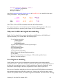
Why use GAMS and algebraic modeling................................................................................. 41
Use of algebraic modeling................................................................................................... 41
Context changes .............................................................................................................. 42
Expandability .................................................................................................................. 42
Augmentation.................................................................................................................. 43
Aid with initial formulation and subsequent changes ......................................................... 44
Adding report writing .......................................................................................................... 44
Self-documenting nature...................................................................................................... 44
Large model facilities .......................................................................................................... 45
Automated problem handling and portability...................................................................... 46
Model library and widespread professional use .................................................................. 46
Use by Others ...................................................................................................................... 46
Courtesy of B.A. McCarl, October 2002
2
Ease of use with NLP, MIP, CGE and other problem forms............................................... 47
Interface with other packages .............................................................................................. 47
Alphabetic list of features ........................................................................................................ 47
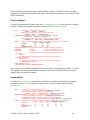
Basic models
In my GAMS short courses I have discovered users approach modeling with at least three
different orientations. These involve users who wish to
Solve objective function oriented constrained optimization problems.
Solve economically based general equilibrium problems.
Solve engineering based nonlinear systems of equations.
In this tutorial I will use three base examples, one from each case hopefully allowing access to
more than one class of user.
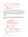
Solving an optimization problem
Many optimization problem forms exist. The simplest of these is the Linear Programming or LP
problem. Suppose I wish to solve the optimization problem
Max 109 * X corn
s.t.
X corn
X corn
X corn
+ 90 * X wheat
+ X wheat
_ 4 * X wheat
X wheat
+ 115 * X Cotton
+ X Cotton
+ 8 * X Cotton
X Cotton
≤ 100
(land )
≤ 500
(labor )
≥ 0 (nonnegativity )
where this is a farm profit maximization problem with three decision variables: Xcorn is the land
area devoted to corn production, Xwheat is the land area devoted to wheat production and Xcotton is
the land area devoted to cotton production. The first equation gives an expression for total profit
as a function of per acre contributions times the acreage allocated by crop and will be
maximized. The second equation limits the choice of the decision variables to the land available
and the third to the labor available. Finally, we only allow positive or zero acreage.
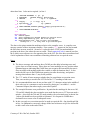
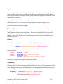
The simplest GAMS formulation of this is (optimize.gms )
VARIABLES
Z;
POSITIVE VARIABLES
Xcorn ,
Xwheat , Xcotton;
EQUATIONS
OBJ, land , labor;
OBJ.. Z =E= 109 * Xcorn + 90 * Xwheat + 115 * Xcotton;
land..
Xcorn +
Xwheat +
Xcotton =L= 100;
labor..
6*Xcorn + 4 * Xwheat + 8 * Xcotton =L= 500;
MODEL farmPROBLEM /ALL/;
SOLVE PROBLEM USING LP MAXIMIZING Z;
Below after introduction of the other two examples I will dissect this formulation explaining its
Courtesy of B.A. McCarl, October 2002
3
components.
Solving for an economic equilibrium
Economists often wish to solve problems that characterize economic equilibria. The simplest of
these is the single good, single market problem. Suppose we wish to solve the equilibrium
problem
Demand Price:
Supply Price:
Quantity Equilibrium:
Non negativity
P > Pd = 6 - 0.3*Qd
P < Ps = 1 + 0.2*Qs
Qs > Qd
P, Qs, Qd > 0
where P is the market clearing price, Pd the demand curve, Qd the quantity demanded, Ps the
supply curve and Qs the quantity supplied. This is a problem in 3 equations and 3 variables (the
variables are P, Qd, and Qs - not Pd and Ps since they can be computed afterwards from the
equality relations).
Ordinarily one would use all equality constraints for such a set up. However, I use this more
general setup because it relaxes some assumptions and more accurately depicts a model ready for
GAMS. In particular, I permit the case where the supply curve price intercept may be above the
demand curve price intercept and thus the market may clear with a nonzero price but a zero
quantity. I also allow the market price to be above the demand curve price and below the supply
curve price. To insure a proper solution in such cases I also impose some additional conditions
based on Walras' law.
Qd*( P - Pd )= 0
Qs*( P – Ps)=0
P*(Qs-Qd)=0
or
or
Qd*(Pd-(6 - 0.3*Qd))=0
Qs*(Ps-( 1 + 0.2*Qs))=0
which state the quantity demanded is nonzero only if the market clearing price equals the
demand curve price, the quantity supplied is nonzero only if the market clearing price equals the
supply curve price and the market clearing price is only nonzero if Qs=Qd.
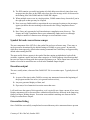
The simplest GAMS formulation of this is below (econequil.gms). Note in this case we needed
to rearrange the Ps equation so it was expressed as a greater than to accommodate the
requirements of the PATH solver.
POSITIVE VARIABLES P, Qd , Qs;
EQUATIONS
Pdemand,Psupply,Equilibrium;
Pdemand..
P
=g= 6 - 0.3*Qd;
Psupply..
( 1 + 0.2*Qs) =g= P;
Equilibrium.. Qs
=g= Qd;
MODEL PROBLEM /Pdemand.Qd,Psupply.Qs,Equilibrium.P/;
SOLVE PROBLEM USING MCP;
Below after introduction of the other example I will dissect this formulation explaining its
components.
Courtesy of B.A. McCarl, October 2002
4
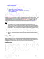
Solving a nonlinear equation system
Engineers often wish to solve a nonlinear system of equations often in a chemical equilibrium or
oil refining context. Many such problem types exist. A simple form of one follows as adapted
from the GAMS model library and the paper Wall, T W, Greening, D, and Woolsey , R E D,
"Solving Complex Chemical Equilibria Using a Geometric-Programming Based Technique".
Operations Research 34, 3 (1987). which is
ba * so4 = 1
baoh / ba / oh = 4.8
hso4 / so4 / h =0 .98
h * oh = 1
ba + 1e-7*baoh = so4 + 1e-5*hso4
2 * ba + 1e-7*baoh + 1e-2*h = 2 * so4 + 1e-5*hso4 + 1e-2*oh
which is a nonlinear system of equations where the variables are ba, so4, baoh, oh, hso4 and h.
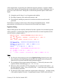
The simplest GAMS formulation of this is (nonlinsys.gms)
Variables ba, so4, baoh, oh, hso4, h ;
Equations r1, r2, r3, r4, b1, b2 ;
r1.. ba * so4 =e= 1 ;
r2.. baoh / ba / oh =e= 4.8 ;
r3.. hso4 / so4 / h =e= .98 ;
r4.. h * oh =e= 1 ;
b1.. ba + 1e-7*baoh =e= so4 + 1e-5*hso4 ;
b2.. 2 * ba + 1e-7*baoh + 1e-2*h =e= 2 * so4 + 1e-5*hso4 + 1e-2*oh ;
Model wall / all / ;
ba.l=1; so4.l=1; baoh.l=1; oh.l=1; hso4.l=1; h.l=1;
Solve wall using nlp minimizing ba;
Dissecting the simple models
Each of the above models is a valid running GAMS program which contains a number of
common and some differentiating language elements. Let us review these elements.
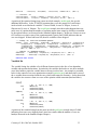
Variables
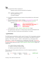
GAMS requires an identification of the variables in a problem. This is accomplished through a
VARIABLES command as reproduced below for each of the three problems.
VARIABLES
POSITIVE VARIABLES
Z;
Xcorn ,Xwheat,Xcotton;
(optimize.gms)
POSITIVE VARIABLES
P, Qd , Qs;
(econequil.gms)
Variables ba, so4, baoh, oh, hso4, h ;
(nonlinsys.gms)
The POSITIVE modifier on the variable definition means that these variables listed thereafter are
Courtesy of B.A. McCarl, October 2002
5
nonnegative i.e. Xcorn , Xwheat , Xcotton, P, Qd , Qs.
The use of the word VARIABLES without the POSITIVE modifier ( note several other
modifiers are possible as discussed in the Variables, Equations, Models and Solves chapter )
means that the named variables are unrestricted in sign as Z, ba, so4, baoh, oh, hso4, and h are
above.
Notes
The general form of these statements are
modifier variables comma or line feed specified list of variables ;
where modifier is optional (positive for example)
variable or variables is required
a list of variables follows
a
; ends the statement
This statement may be more complex including set element definitions (as we will
elaborate on below) and descriptive text as illustrated in the file (model.gms)
Variables
Tcost
Binary Variables
Build(Warehouse)
Positive Variables
Shipsw(Supplyl,Warehouse)
Shipwm(Warehouse,Market)
Shipsm(Supplyl,Market)
Semicont Variables
X,y,z;
‘ Total Cost Of Shipping- All Routes’;
Warehouse Construction Variables;
Shipment to warehouse
Shipment from Warehouse
Direct ship to Demand;
as discussed in the Variables, Equations, Models and Solves chapter.
The variable names can be up to 31 characters long as discussed and illustrated in the
Rules for Item Names, Element names and Explanatory Text chapter.
GAMS is not case sensitive, thus it is equivalent to type the command VARIABLE as
variable or the variable names XCOTTON as XcOttoN. However, there is case
sensitivity with respect to the way things are printed out with the first presentation being
the one used as discussed in the Rules for Ordering and Capitalization chapter.
GAMS does not care about spacing or multiple lines. Also a line feed can be used
instead of a comma. Thus, the following three command versions are all the same
POSITIVE VARIABLES
Xcorn ,Xwheat,Xcotton;
Positive Variables
Xcorn,
Xwheat,
Xcotton;
positive variables
Xcorn
Xwheat
Courtesy of B.A. McCarl, October 2002
,
Xcotton;
6
What is the new Z variable in the optimization problem?
In the optimization problem I had three variables as it was originally stated but in the GAMS
formulation I have four. Why? GAMS requires all optimization models to be of a special form.
Namely, given the model
Maximize cx
It must be rewritten as
Maximize
R
R=CX
where R is a variable unrestricted in sign. This variable can be named however you want it
named (in the above example case Z). There always must be at least one of these in every
problem which is the objective function variable and it must be named as the item to maximize
or minimize.
Thus in a problem one needs to declare a new unrestricted variable and define it though an
equation. In our optimization example (optimize.gms) we declared Z as a Variable (not a
Positive Variable), then we declared and specified an equation setting Z equal to the objective
function expression and told the solver to maximize Z,
VARIABLES
Z;
EQUATIONS
OBJ, land , labor;
OBJ.. Z =E=
109 * Xcorn + 90 * Xwheat + 115 * Xcotton;
SOLVE PROBLEM USING LP MAXIMIZING Z;
Note users do not always have to add such an equation if there is a variable in the model that is
unrestricted in sign that can be used as the objective function. For example the equation solving
case (nonlinsys.gms) uses a maximization of ba as a dummy objective function (as further
discussed below the problem is really designed to just solve the nonlinear system of equations
and the objective is just there because the model type used needed one).
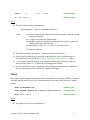
Equations
GAMS requires that the modeler name each equation, which is active in the optimization model.
Later each equation is specified using the .. notation as explained just below. These equations
must be named in an EQUATION or EQUATIONS instruction. This is used in each of the
example models as reproduced below
EQUATIONS
OBJ,
land ,
labor;
EQUATIONS
PDemand,PSupply, Equilibrium;
Equations r1, r2, r3, r4, b1, b2 ;
Courtesy of B.A. McCarl, October 2002
(optimize.gms)
(econequil.gms)
(nonlinsys.gms)
7
Notes
The general form of these statements are
Equations comma or line feed specified list of equations ;
where equation or equations is required
a list of equations follows
a
; ends the statement
In optimization models the objective function is always defined in one of the named
equations.
This statement may be more complex including set element definitions (as we will
elaborate on below) and descriptive text as illustrated in the file (model.gms)
EQUATIONS
TCOSTEQ
SUPPLYEQ(SUPPLYL)
DEMANDEQ(MARKET)
BALANCE(WAREHOUSE)
CAPACITY(WAREHOUSE)
CONFIGURE
TOTAL COST ACCOUNTING EQUATION
LIMIT ON SUPPLY AVAILABLE AT A SUPPLY POINT
MINIMUM REQUIREMENT AT A DEMAND MARKET
WAREHOUSE SUPPLY DEMAND BALANCE
WAREHOUSE CAPACITY
ONLY ONE WAREHOUSE;
as discussed in the Variables, Equations, Models and Solves chapter.
The equation names can be up to 31 characters long as discussed and illustrated in the
Rules for Item Names, Element names and Explanatory Text chapter.
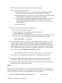
.. specifications
The GAMS equation specifications actually consist of two parts. The first part naming equations,
was discussed just above. The second part involves specifying the exact algebraic structure of
equations. This is done using the .. notation. In this notation we give the equation name
followed by a .. then the exact equation type as it should appear in the model. The equation
type specification involves use of a special syntax to tell the exact form of the relation involved.
The most common of these are (see the Variables, Equations, Models and Solves chapter for a
complete list):
=E= is used to indicate an equality relation
=L= indicates a less than or equal to relation
=G= indicates a greater than or equal to relation
This is used in each of the example models where a few of the component equations are
reproduced below
OBJ.. Z =E= 109*Xcorn + 90*Xwheat + 115*Xcotton;
land..
Xcorn +
Xwheat +
Xcotton =L= 100;
Courtesy of B.A. McCarl, October 2002
(optimize.gms)
8
Pdemand..
r1..
P
=g= 6 - 0.3*Qd;
(econequil.gms)
(nonlinsys.gms)
ba * so4 =e= 1 ;
Notes
The general form of these statements are
Equationname
where
..
algebra1 equationtype algebra2 ;
an equation with that name must have been declared (have appeared in and
equation statement)
..
the appears just after the equation name
the algebraic expressions algebra1 and algebra2 can each be a mixture of
variables, data items and constants
the equationtype is the =E=, =L=, and =G= discussed above.
a
; ends the statement
All equations must be specified in .. notation before they can be used.
Some model equations may be specified in an alternative way by including upper or
lower bounds as discussed in the Variables, Equations, Models and Solves chapter.
.. specification statements may be more complex including more involved algebra as
discussed later in this tutorial and in the Calculating Items chapter.
It may be desirable to express equations as only being present under some conditions as
discussed later in this tutorial and in the Conditionals chapter.
Model
Once all the model structural elements have been defined then one employs a MODEL statement
to identify models that will be solved. Such statements occur in the each of the three example
models:
MODEL farmPROBLEM /ALL/;
(optimize.gms)
MODEL PROBLEM /Pdemand.Qd, Psupply.Qs,Equilibrium.P/;
(econequil.gms)
Model wall / all / ;
(nonlinsys.gms)
Notes
The general form of these statements are
Courtesy of B.A. McCarl, October 2002
9
Model modelname optional explanatory text / model contents/ ;
where Model or models is required
a modelname follows that can be up to 31 characters long as discussed in the
Rules for Item Names, Element names and Explanatory Text chapter
the optional explanatory text is up to 255 characters long as discussed in the Rules
for Item Names, Element names and Explanatory Text chapter
the model contents are set off by beginning and ending slashes and can either be
the keyword all including all equations, a list of equations, or a list of
equations and complementary variables. Each of these is discussed in the
following bullets.
a
; ends the statement
In the Model Statement in the model contents field
Using /ALL/ includes all the equations.
One can list equations in the model statement like that below.
MODEL FARM /obj, Land,labor/;
and one does not need to list all the equations listed in the Equations statements. Thus
in (optimize.gms) one could omit the constraints called labor from the model
MODEL ALTPROBLEM / obj,land/;
The equilibrium problems are solved as Mixed complementarity problems (MCP) and
require a special variant of the Model statement. Namely in such problems there are
exactly as many variables as there are equations and each variable must be specified as
being complementary with one and only one equation. The model statement expresses
these constraints indicating the equations to be included followed by a period(.) and the
name of the associated complementary variables as follows
MODEL PROBLEM /Pdemand.Qd, Psupply.Qs,Equilibrium.P/; (econequil.gms)
which imposes the complementary relations form our equilibrium problem above.
All equations in the model which are named and any data included must have been
specified in .. notation before this model can be used (in a later solve statement).
Users may create several models in one run each containing a different set of equations
and then solve those models and separately.
Solve
Once one believes that the model is ready in such that it makes sense to find a solution for the
variables then the solve statement comes into play. The SOLVE statement causes GAMS to use
a solver to optimize the model or solve the embodied system of equations.
SOLVE farmPROBLEM USING LP MAXIMIZING Z;
Courtesy of B.A. McCarl, October 2002
(optimize.gms)
10
SOLVE PROBLEM USING MCP;
(econequil.gms)
Solve wall using nlp minimizing ba;
(nonlinsys.gms)
Notes
The general forms of these statements for models with objective functions are
Solve modelname using modeltype maximizing variablename ;
Solve modelname using modeltype minimizing variablename ;
and for models without objective functions is
Solve modelname using modeltype;
where Solve is required
a modelname follows that must have already been given this name in a Model
statement
using is required
the modeltype is one of the known GAMS model types where
♦ models with objective functions are
LP for linear programming
NLP for nonlinear programming
MIP for mixed integer programming
MINLP for mixed integer non linear programming
plus RMIP, RMINLP, DNLP, MPEC as discussed in the chapter on Model
Types and Solvers.
♦ models without objective functions are
MCP for mixed complementary programming
CNS for constrained nonlinear systems
maximizing or minimizing is required for all optimization problems (not MCP or
CNS problems)
a variablename to maximize or minimize is required for all optimization problems
(not MCP or CNS problems) and must match with the name of a variable defined as
free or just as a variable.
a
; ends the statement
The examples statement solve three different model types
Courtesy of B.A. McCarl, October 2002
11
a linear programming problem (“using LP”).
a mixed complementary programming problem (“using MCP”).
a non linear programming problem (“using NLP”).
GAMS does not directly solve problems. Rather it interfaces with external solvers
developed by other companies. This requires special licensing arrangements to have
access to the solvers. It also requires that for the user to use a particular solver that it all
ready must have been interfaced with GAMS. A list of the solvers currently interfaced is
covered in the Model Types and Solvers chapter.
Why does my nonlinear equation system maximize something?
The nonlinear equation system chemical engineering problem in the GAMS formulation was
expressed as a nonlinear programming (NLP) optimization model in turn requiring an objective
function. Actually this is somewhat older practice in GAMS as the constrained nonlinear system
(CNS) model type was added after this example was initially formulated. Thus, one could
modify the model type to solve constrained nonlinear system yielding the same solution using
Solve wall using mcp;
(nonlinsyscns.gms).
However, the CNS model type can only be solved by select solvers and cannot incorporate
integer variables. Formulation as an optimization problem relaxes these restrictions allowing use
of for example the MINLP model type plus the other NLP solvers. Such a formulation involves
the choice of a convenient variable to optimize which may not really have any effect since a
feasible solution requires all of the simultaneous equations to be solved. Thus while ba is
maximized there is no inherent interest in attaining its maximum it is just convenient.
What are the .L items
In the nonlinear equation system chemical engineering GAMS formulation a line was introduced
which is
ba.l=1; so4.l=1; baoh.l=1; oh.l=1; hso4.l=1; h.l=1;
(nonlinsys.gms)
This line provides a starting point for the variables in the model. In particular the notation
variablename.l=value is the way one introduces a starting value for a variable in GAMS as
discussed in the chapter on NLP and MCP Model Types. Such a practice can be quite important
in achieving success and avoiding numerical problems in model solution (as discussed in the
Execution Errors chapter).
Notes
One may also need to introduce lower (variablename.lo=value ) and upper
(variablename.up=value ) bounds on the variables as also discussed in the Execution
Errors chapter.
Courtesy of B.A. McCarl, October 2002
12
The .l, .lo and .up appendages on the variable names are illustrations of variable attributes
as discussed in the Variables, Equations, Models and Solves chapter.
The = statements setting the variable attributes to numbers are the first example we have
encountered of a GAMS assignment statement as extensively discussed in the Calculating
Items chapter.
Running the job
GAMS is a two pass program. One first uses an editor to create a file nominally with the
extension GMS which contains GAMS instructions. Later when the file is judged complete one
submits that file to GAMS. In turn, GAMS executes those instructions causing calculations to be
done, solvers to be used and a solution file of the execution results to be created. Two
alternatives for submitting the job exist the traditional command line approach and the IDE
approach.
Command line approach
The basic procedure involved for running command line GAMS is to create a file (nominally
myfilename.gms where myfilename is whatever is a legal name on the operating system being
used) with a text editor and when done run it with a DOS or UNIX or other operating system
command line instruction like
GAMS trnsport
where trnsport.gms is the file to be run. Note the gms extension may be omitted and GAMS will
still find the file.
The basic command line GAMS call also allows a number of arguments as illustrated below
GAMS TRNSPORT pw=80 ps=9999 s=mysave
which sets the page width to 80, the page length to 9999 and saves work files. The full array of
possible command line arguments is discussed in the GAMS Command Line Parameters chapter.
When GAMS is run the answers are placed in the LST file. Namely if the input file of GAMS
instructions is called myfile.gms then the output will be on myfile.LST.
IDE approach
Today with the average user becoming oriented to graphical interfaces it was a natural
development to create the GAMSIDE or IDE for short. The IDE is a GAMS Corporation
product providing an Integrated Development Environment that is designed to provide a
Windows graphical interface to allow for editing, development, debugging, and running of
GAMS jobs all in one program. I will not cover IDE usage in this tutorial and rather refer the
reader to the tutorial on IDE usage that appears in the chapter on Running Jobs with GAMS and
the GAMS IDE. When the IDE is run there is again the creation of the LST file. Namely if the
Courtesy of B.A. McCarl, October 2002
13
input file of GAMS instructions is called myfile.gms then the output will be on myfile.LST.
Examining the output
When a GAMS file is run then GAMS in turn creates a LST file of problem results. One can edit
the LST file in either the IDE or with a text editor to find any error messages, solution output,
report writing displays etc. In turn one can also reedit the GMS file if there were need to fix
anything or alter the model contents and rerun with GAMS until a satisfactory result is attained.
Now let us review the potential elements of the LST file.
Echo print
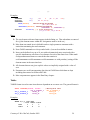
The first item contained within the LST file is the echo print. The echo print is simply a
numbered copy of the instructions GAMS received in the GMS input file. For example, in the
LST file segment immediately below is the portion associated with the GAMS instructions in
optimize.gms.
3
4
5
6
7
8
9
10
VARIABLES
Z;
POSITIVE VARIABLES
Xcorn ,
Xwheat , Xcotton;
EQUATIONS
OBJ, land , labor;
OBJ.. Z =E= 109 * Xcorn + 90 * Xwheat + 115 * Xcotton;
land..
Xcorn +
Xwheat +
Xcotton =L= 100;
labor..
6*Xcorn + 4 * Xwheat + 8 * Xcotton =L= 500;
MODEL farmPROBLEM /ALL/;
SOLVE farmPROBLEM USING LP MAXIMIZING Z;
Notes
The echo print is of the same character for all three examples so I only include the
optimize.gms LST file echo print here.
The echo print can incorporate lines from other files if include files are present as
covered in the Including External Files chapter.
The echo print can be partially or fully suppressed as discussed in the Standard Output
chapter.
The numbered echo print often serves as an important reference guide because GAMS
reports the line numbers in the LST file where solves or displays were located as well as
a the position of any errors that have been encountered.
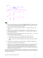
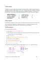
Incidence of compilation errors
GAMS requires strict adherence to language syntax. It is very rare for even experienced users to
get their syntax exactly right the first time. GAMS marks places where syntax does not
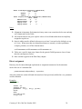
correspond exactly as compilation errors in the echo print listing. For example I present the echo
print from a syntactically incorrect variant of the economic equilibrium problem. In that
example (econequilerr.gms) I have introduced errors in the form of a different spelling of the
variable named Qd between line's 1, 3, 5 and 6 spelling it as Qd in line 1 and Qdemand in the
Courtesy of B.A. McCarl, October 2002
14
other three lines. I also omit a required ; in line 4.
1
2
3
****
4
5
****
6
****
7
****
POSITIVE VARIABLES P, Qd , Qs;
EQUATIONS
PDemand,PSupply, Equilibrium;
Pdemand..
P
=g= 6 - 0.3*Qdemand;
$140
Psupply..
( 1 + 0.2*Qs) =g= P
Equilibrium.. Qs
=g= Qdemand;
$409
MODEL PROBLEM /Pdemand.Qdemand, Psupply.Qs,Equilibrium.P/;
$322
SOLVE PROBLEM USING MCP;
$257
Error Messages
140 Unknown symbol
257 Solve statement not checked because of previous errors
322 Wrong complementarity pair. Has to be equ.var.
409 Unrecognizable item - skip to find a new statement
looking for a ';' or a key word to get started again
The above echo print contains the markings relative to the compiler errors. A compiler error
message consists of three important elements. First a marker **** appears in line just beneath
the line where an error occurred. Second a $ is placed in the LST file just underneath the
position in the above line where the error occurred. Third a numerical code is entered just after
the $ which cross-references to a list appearing later in the LST file of the heirs encountered and
a brief explanation of their cause sometimes containing a hint on how to repair the error.
Notes
The above messages and markings show GAMS provides help in locating errors and
givies clues as to what's wrong. Above there are error markings in every position where
Qdemand appears indicating that GAMS does not recognize the item mainly because it
does not match with anything within the variable or other declarations above. It also
marks the 409 error in the Equilibrium equation just after the missing ; and prints a
message that indicates that a ; may be the problem.
The **** marks all error messages whether they be compilation or execution errors.
Thus, one can always search in the LST file for the **** marking to find errors.
It is recommended that users do not use lines with **** character strings in the middle of
their code (say in a comment as can be entered by placing an * in column 1—see the
Comments chapter) but rather employ some other symbol.
The example illustrates error proliferation. In particular the markings for the errors 140,
322 and 409 identify the places mistakes were made but the error to 257 does not mark a
mistake. Also while the 140 and 322 mark mistakes, the real mistake may be that in line
1 where Qd should have been spelled as Qdemand. It is frequent in GAMS that a
declaration error causes a lot of subsequent errors.
In this case only two corrections need to be made to repair the file. One should spell Qd
in line 1 as Qdemand or conversely change all the later references to Qd. One also needs
to add a semi colon to the end of line 4.
Courtesy of B.A. McCarl, October 2002
15
The IDE contains a powerful navigation aid which helps users directly jump from error
messages into the place in the GMS code where the error message occurs as discussed in
the Running Jobs with GAMS and the GAMS IDE chapter.
When multiple errors occur in a single position, GAMS cannot always locate the $ just in
the right spot as that spot may be occupied.
New users may find desirable to reposition the error message locations so the messages
appear just below the error markings as discussed in the Fixing Compilation Errors
chapter.
Here I have only presented a brief introduction to compilation error discovery. The
chapter on Fixing Compilation Errors goes substantially further and covers through
example a number of common error messages received and their causes.
Symbol list and cross reference maps
The next component of the LST file is the symbol list and cross-reference map. These may or
not be present as determined by the default settings of GAMS on your system. In particular,
while these items appear by default when running command line GAMS they are suppressed by
default when running the IDE.
The more useful of these outputs is the symbol list that contains an alphabetical order all the
variables, equations, models and some other categories of GAMS language classifications that I
have not yet discussed along with their optional explanatory text. These output items will not be
further covered in its tutorial but are covered in the Standard Output chapter.
Execution output
The next, usually minor, element of the GAMS LST file is execution report. Typically this will
involve
A report of the time it takes GAMS to execute any statements between the beginning of
the program and the first solve (or in general between solves),
Any user generated displays of data; and
If present, a list of numerical execution errors that arose.
I will not discuss the nature of this output here, as it is typically not a large concern of new users.
Display statements will be discussed later within this tutorial and are discussed in the Improving
Output via Report Writing chapter. Execution errors and their markings are discussed in the
Fixing Execution Errors chapter.
Generation listing
Once GAMS has successfully compiled and executed then any solve statements that are present
Courtesy of B.A. McCarl, October 2002
16
will be implemented. In particular, the GAMS main program generates a computer readable
version of the equations in the problem that it in turn passes on to whatever third party solver is
going to be used on the model. During this so called model generation phase GAMS creates
output
Listing the specific form of a set of equations and variables,
Providing a summary of the total model structure, and
If encountered, detailing any numerical execution errors that occurred in model
generation.
Each of these excepting execution errors will be discussed immediately below. Model
generation time execution errors are discussed in the Execution Errors chapter.
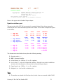
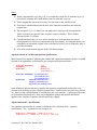
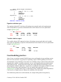
Equation listing
When GAMS generates the model by default the first three equations for each named equation
will be generated. A portion of the output (just that for the first two named equations) for the
each for the three example models is
Equation Listing
SOLVE farmPROBLEM Using LP From line 10
---- OBJ =E=
OBJ.. Z - 109*Xcorn - 90*Xwheat - 115*Xcotton =E= 0 ; (LHS = 0)
---- land =L=
land.. Xcorn + Xwheat + Xcotton =L= 100 ; (LHS = 0)
Equation Listing
SOLVE wall Using NLP From line 28
---- PDemand =G=
PDemand.. P + 0.3*Qd =G= 6 ; (LHS = 0, INFES = 6 ***)
---- PSupply =G=
PSupply.. - P + 0.2*Qs =G= -1 ; (LHS = 0)
Equation Listing
SOLVE PROBLEM Using MCP From line 7
---- r1 =E=
r1.. (1)*ba + (1)*so4 =E= 1 ; (LHS = 1)
---- r2 =E=
r2.. - (1)*ba + (1)*baoh - (1)*oh =E= 4.8 ; (LHS = 1, INFES = 3.8 ***)
Notes
The first part of this output gives the words Equation Listing followed by the word
Solve, the name of the model being solved and the line number in the echo print file
where the solve associated with this model generation appears.
The second part of this output consists of the marker ---- followed by the name of the
equation with the relationship type (=L=, =G=, =E= etc).
When one wishes to find this LST file component, one can search for the marker ---- or
the string Equation Listing. Users will quickly find ---- marks other types of output like
that from display statements.
The third part of this output contains the equation name followed by a .. and then a listing
of the equation algebraic structure. In preparing this output, GAMS collects all terms
Courtesy of B.A. McCarl, October 2002
17
involving variables on the left hand side and all constants on the right hand side. This
output component portrays the equation in linear format giving the names of the variables
that are associated with nonzero equation terms and their associated coefficients.
The algebraic structure portrayal is trailed by a term which is labeled LHS and gives at
evaluation of the terms involving endogenous variables evaluated at their starting points
(typically zero unless the .L levels were preset). A marker INFEAS will also appear if
the initial values do not constitute a feasible solution.
The equation output is a correct representation of the algebraic structure of any linear
terms in the equation and a local representation containing the first derivatives of any
nonlinear terms. The nonlinear terms are automatically encased in parentheses to
indicate a local approximation is present. For example in the non-linear equation solving
example the first equation is algebraically structured as
ba * so4 = 1
but the equation listing portrays this as additive
---- r1 =E=
r1.. (1)*ba + (1)*so4 =E= 1 ; (LHS = 1)
which the reader can verify as the first derivative use of the terms evaluated around the
starting point (ba=1,so4=1).
More details on how the equation list is formed and controlled in terms of content and length are
discussed in the Standard Output chapter while more on nonlinear terms appears in the NLP and
MCP Model Types chapter.
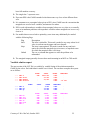
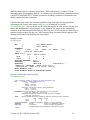
Variable listing
When GAMS generates the model by default the first three variables for each named variable
will be generated. A portion of the output (just that for the first two named variables) for the
each for the three example models is
Column Listing
---- Z
Z
1
---- Xcorn
Xcorn
-109
1
6
Column Listing
---- P
P
1
-1
SOLVE farmPROBLEM Using LP From line 10
(.LO, .L, .UP = -INF, 0, +INF)
OBJ
(.LO, .L, .UP = 0, 0, +INF)
OBJ
land
labor
SOLVE PROBLEM Using MCP From line 7
(.LO, .L, .UP = 0, 0, +INF)
PDemand
PSupply
Courtesy of B.A. McCarl, October 2002
18
---- Qd
Qd
0.3
-1
Column Listing
---- ba
ba
(1)
(-1)
1
2
---- so4
so4
(1)
(-1)
-1
-2
(.LO, .L, .UP = 0, 0, +INF)
PDemand
Equilibrium
SOLVE wall Using NLP From line 28
(.LO, .L, .UP = -INF, 1, +INF)
r1
r2
b1
b2
(.LO, .L, .UP = -INF, 1, +INF)
r1
r3
b1
b2
Notes
The first part of this output gives the words Column Listing followed by the word Solve,
the name of the model being solved and the line number in the echo print file where the
solve associated with this model generation appears.
The second part of this output consists of the marker ---- followed by the name of the
variable.
When one wishes to find this LST file component, one can search for the marker ---- or
the string Column Listing. Users will quickly find ---- marks other types of output like
that from display statements.
The third part of this output contains the variable name followed by (.LO, .L, .UP = lower
bound, starting level, upper bound) where
lower bound gives the lower bound assigned to this variable (often zero)
starting level gives the starting point assigned to this variable (often zero)
upper bound gives the lower bound assigned to this variable (often positive infinity +
INF).
The fourth part of this output gives the equation names in which this variable appears
with a nonzero term and the associated coefficients.
The output is a correct representation of the algebraic structure of any linear terms in the
equations where the variable appears and a local representation containing the first
derivatives of any nonlinear terms. The nonlinear terms are automatically encased in
parentheses to indicate a local approximation is present just analogous to the portrayals in
the equation listing section just above.
More details on how the variable list is formed and controlled in terms of content and length are
discussed in the Standard Output chapter while more on nonlinear terms appears in the NLP and
MCP Model Types chapter.
Courtesy of B.A. McCarl, October 2002
19
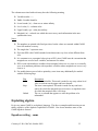
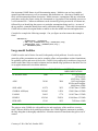
Model statistics
GAMS also creates an output summarizing the size of the model as appears just below from the
non-linear equation solving example nonlinsys.gms. This gives how many variables of equations
and nonlinear terms are in the model along with some additional information. For discussion of
the other parts of this output see the Standard Output and NLP and MCP model types chapters.
MODEL STATISTICS
BLOCKS OF EQUATIONS
BLOCKS OF VARIABLES
NON ZERO ELEMENTS
DERIVATIVE POOL
CODE LENGTH
6
6
20
6
89
SINGLE EQUATIONS
SINGLE VARIABLES
NON LINEAR N-Z
CONSTANT POOL
6
6
10
8
Solver report
The final major component of the LST file is the solution output and consists of a summary and
then a report of the solutions for variables and equations. Execution error reports may also
appear in nonlinear models as discussed in the Execution Errors Chapter.
Solution summary
The solution summary contains
the marker S O L V E
S U M M A R Y;
the model name, objective variable name (if present), optimization type (if present), and
location of the solve (in the echo print);
the solver name;
the solve status in terms of solver termination condition;
the objective value (if present);
some cpu time expended reports;
a count of solver execution errors; and
some solver specific output.
The report from the non-linear equation solving example nonlinsys.gms appears just below.
S O L V E
MODEL
TYPE
SOLVER
S U M M A R Y
wall
NLP
CONOPT
**** SOLVER STATUS
**** MODEL STATUS
**** OBJECTIVE VALUE
OBJECTIVE
DIRECTION
FROM LINE
ba
MINIMIZE
28
1 NORMAL COMPLETION
2 LOCALLY OPTIMAL
1.0000
Courtesy of B.A. McCarl, October 2002
20
RESOURCE USAGE, LIMIT
ITERATION COUNT, LIMIT
EVALUATION ERRORS
0.090
5
0
1000.000
10000
0
C O N O P T 2
Copyright (C)
Windows NT/95/98 version 2.071J-011-046
ARKI Consulting and Development A/S
Bagsvaerdvej 246 A
DK-2880 Bagsvaerd, Denmark
Using default control program.
** Optimal solution. There are no superbasic variables.
More on this appears in the Standard Output chapter.
Equation solution report
The next section of the LST file is an equation by equation listing of the solution returned to
GAMS by the solver. Each individual equation case is listed. For our three examples the reports
are as follows
---- EQU OBJ
---- EQU land
---- EQU labor
LOWER
.
-INF
-INF
LEVEL
.
100.000
500.000
UPPER
.
100.000
500.000
MARGINAL
1.000
52.000
9.500
---- EQU PDemand
---- EQU PSupply
---- EQU Equilibri~
LOWER
6.000
-1.000
.
LEVEL
6.000
-1.000
.
UPPER
+INF
+INF
+INF
MARGINAL
10.000
10.000
3.000
-------------------
LOWER
1.000
4.800
0.980
1.000
.
.
LEVEL
1.000
4.800
0.980
1.000
.
.
UPPER
MARGINAL
1.000
0.500
4.800
EPS
0.980 4.9951E-6
1.000 2.3288E-6
.
0.499
.
2.5676E-4
EQU
EQU
EQU
EQU
EQU
EQU
r1
r2
r3
r4
b1
b2
The columns associated with each entry have the following meaning,
Equation marker ---EQU - Equation identifier
Lower bound (.lo) – RHS on =G= or =E= equations
Level value (.l) – value of Left hand side variables. Note this is not a slack variable but
inclusion of such information is discussed in the Standard Output chapter.
Upper bound (.up) – RHS on =L= or =E= equations
Marginal (.m) – dual variable or shadow price
Notes
The numbers are printed with fixed precision, but the values are returned within GAMS
Courtesy of B.A. McCarl, October 2002
21
have full machine accuracy.
The single dots '.' represent zeros.
If present EPS is the GAMS extended value that means very close to but different from
zero.
It is common to see a marginal value given as EPS, since GAMS uses the convention that
marginals are zero for basic variables, and nonzero for others.
EPS is used with non-basic variables whose marginal values are very close to, or actually,
zero, or in nonlinear problems with superbasic variables whose marginals are zero or very
close to it.
For models that are not solved to optimality, some items may additionally be marked
with the following flags.
Flag
Infes
Description
The item is infeasible. This mark is made for any entry whose level
value is not between the upper and lower bounds.
The item is non-optimal. This mark is made for any non-basic
entries for which the marginal sign is incorrect, or superbasic ones
for which the marginal value is too large.
The row or column that appears to cause the problem to be
unbounded.
Nopt
Unbnd
The marginal output generally does not have much meaning in an MCP or CNS model.
Variable solution report
The next section of the LST file is a variable by variable listing of the solution returned to
GAMS by the solver. Each individual variable case is listed. For our three examples the reports
are as follows
-------------
VAR
VAR
VAR
VAR
Z
Xcorn
Xwheat
Xcotton
---- VAR P
---- VAR Qd
---- VAR Qs
-------------------
VAR
VAR
VAR
VAR
VAR
VAR
ba
so4
baoh
oh
hso4
h
LOWER
LOWER
-INF
.
.
.
LEVEL
.
.
.
LOWER
-INF
-INF
-INF
-INF
-INF
-INF
Courtesy of B.A. McCarl, October 2002
LEVEL
9950.000
50.000
50.000
.
UPPER
3.000
10.000
10.000
LEVEL
1.000
1.000
4.802
1.000
0.980
1.000
UPPER
+INF
+INF
+INF
+INF
MARGINAL
.
.
.
-13.000
MARGINAL
+INF
+INF
+INF
UPPER
+INF
+INF
+INF
+INF
+INF
+INF
.
.
.
MARGINAL
.
.
.
.
.
.
22
The columns associated with each entry have the following meaning,
Variable marker ---VAR - Variable identifier
Lower bound (.lo) – often zero or minus infinity
Level value (.l) – solution value.
Upper bound (.up) – often plus infinity
Marginal (.m) – reduced cost which does not convey much information in the non
optimization cases,
Notes
The numbers are printed with fixed precision, but the values are returned within GAMS
have full machine accuracy.
The single dots '.' represent zeros.
If present EPS is the GAMS extended value that means very close to but different from
zero.
It is common to see a marginal value given as EPS, since GAMS uses the convention that
marginals are zero for basic variables, and nonzero for others.
EPS is used with non-basic variables whose marginal values are very close to, or actually,
zero, or in nonlinear problems with superbasic variables whose marginals are zero or very
close to it.
For models that are not solved to optimality, some items may additionally be marked
with the following flags.
Flag
Infes
Nopt
Unbnd
Description
The item is infeasible. This mark is made for any entry whose level
value is not between the upper and lower bounds.
The item is non-optimal. This mark is made for any non-basic
entries for which the marginal sign is incorrect, or superbasic ones
for which the marginal value is too large.
The row or column that appears to cause the problem to be
unbounded.
Exploiting algebra
By its very nature GAMS is an algebraic language. The above examples and discussion are not
totally exploitive of the algebraic capabilities of GAMS. Now let me introduce more of the
GAMS algebraic features.
Equation writing – sums
Courtesy of B.A. McCarl, October 2002
23
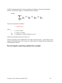
GAMS is fundamentally built to allow exploitation of algebraic features like summation
notation. Specifically suppose xi is defined with three elements
Algebra
∑x
i
= x1 + x 2 + x3
i
This can be expressed in GAMS as
z = SUM(I, X(I));
where
I
z
X(I)
is a set in GAMS
is a scalar or variable
is a parameter or variable defined over set I
and the sum automatically treats all cases of I.
Such an expression can be included either in a either a model equation .. specification or in an
item to be calculated in the code. Let me now remake the first 2 examples better exploiting the
GAMS algebraic features
Revised algebra exploiting optimization example
Courtesy of B.A. McCarl, October 2002
24
The optimization example is as follows
Max 109 * X corn
s.t.
X corn
X corn
X corn
+ 90 * X wheat
+ X wheat
+ 115 * X Cotton
+ X Cotton
_ 4 * X wheat
X wheat
+ 8 * X Cotton
X Cotton
≤ 100
(land )
≤ 500
(labor )
≥ 0 (nonnegativity )
This is a special case of the general resource allocation problem that can be written as
Max
∑C X
∑a X
j
j
ij
j
j
s.t.
j
Xj
≤ bi
for all i
≥
for all j
0
where
j=
i=
xj =
cj =
aij =
{
{
{
{
bi =
{
corn
land
Xcorn
109
1
6
100
Xwheat
90
wheat cotton }
labor }
Xcotton }
115
}
1
4
500
}’
1
8
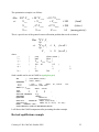
Such a model can be cast in GAMS as (optalgebra.gms)
SET
j
i
/Corn,Wheat,Cotton/
/Land ,Labor/;
PARAMETER
c(j)
/ corn
109
,wheat
90 ,cotton
115/
b(i)
/land 100 ,labor 500/;
TABLE a(i,j)
corn
wheat
cotton
land
1
1
1
labor
6
4
8
;
POSITIVE VARIABLES
x(j);
VARIABLES
PROFIT
;
EQUATIONS
OBJective
,
constraint(i) ;
OBJective..
PROFIT=E=
SUM(J,(c(J))*x(J)) ;
constraint(i)..
SUM(J,a(i,J) *x(J)) =L= b(i);
MODEL
RESALLOC /ALL/;
SOLVE RESALLOC USING LP MAXIMIZING PROFIT;
I will dissect the GAMS components after presenting the other example.
Revised equilibrium example
Courtesy of B.A. McCarl, October 2002
25
The economic equilibrium model was of the form
Demand Price:
P > Pd = 6 - 0.3*Qd
Supply Price:
P < Ps = 1 + 0.2*Qs
Quantity Equilibrium:
Qs > Qd
Non negativity
P, Qs, Qd > 0
and is a single commodity model. Introduction of multiple commodities means that we need a
subscript for commodities and consideration of cross commodity terms in the functions. Such a
formulation where c depicts commodity can be presented as
Demand Price for c:
Supply Price for c:
Quantity Equil. for c:
Non negativity
Pc
≥ Pd c = Id c - ∑ Sd c,cc * Qd cc
for all c
Pc
≤ Ps c = Is c + ∑ Ss c,cc * Qs cc
for all c
cc
cc
Qs c ≥ Qd c
Pc , Qd c , Qs c ≥ 0
for all c
for all c
where Pc is the price of commodity c
Qdc is the quantity demanded of commodity c
Pdc is the price from the inverse demand curve for commodity c
Qsc is the quantity supplied of commodity c
Psc is the price from the inverse supply curve for commodity c
cc is an alternative index to the commodities and is equivalent to c
Idc is the inverse demand curve intercept for c
Ddc,cc is the inverse demand curve slope for the effect of buying one unit of commodity
cc on the demand price of commodity c. When c=cc this is an own commodity
effect and when c≠cc then this is a cross commodity effect.
Isc is the inverse supply curve intercept for c
Dsc,cc is the inverse supply curve slope for the effect of supplying one unit of commodity
cc on the supply price of commodity c. When c=cc this is an own commodity effect
and when c≠cc then this is a cross commodity effect.
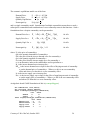
An algebraic based GAMS formulation of this is (econequilalg.gms)
Set commodities /corn,wheat/;
Set curvetype /Supply,demand/;
Table intercepts(curvetype,commodities)
corn
wheat
demand
4
8
supply
1
2;
table slopes(curvetype,commodities,commodities)
corn wheat
demand.corn
-.3
-.1
demand.wheat -.07
-.4
supply.corn
.5
.1
supply.wheat
.1
.3
;
Courtesy of B.A. McCarl, October 2002
26
POSITIVE VARIABLES
P(commodities)
Qd(commodities)
Qs(commodities) ;
EQUATIONS
PDemand(commodities)
PSupply(commodities)
Equilibrium(commodities) ;
alias (cc,commodities);
Pdemand(commodities)..
P(commodities)=g=
intercepts("demand",commodities)
+sum(cc,slopes("demand",commodities,cc)*Qd(cc));
Psupply(commodities)..
intercepts("supply",commodities)
+sum(cc,slopes("supply",commodities,cc)* Qs(cc))
=g= P(commodities);
Equilibrium(commodities)..
Qs(commodities)=g= Qd(commodities);
MODEL PROBLEM /Pdemand.Qd, Psupply.Qs,Equilibrium.P/;
SOLVE PROBLEM USING MCP;
Dissecting the algebraic model
Sets
Above we used the subscripts i , j, commodities and cc for addressing the variable, equation and
data items. In GAMS subscripts are SETs. In order to use any subscript one must declare an
equivalent set.
The set declaration contains
the set name
a list of elements in the set (up to 31 characters long spaces etc allowed in quotes)
optional labels describing the whole set
optional labels defining individual set elements
The general format for a set statement is:
SET setname
/
optional defining text
firstsetelementname
optional defining text
secondsetelementname
optional defining text
... /;
Examples
(sets.gms)
SETs
SET
SET
j
i
/x1,x2,x3/
/r1 ,r2/;
PROCESS
PRODUCTION PROCESSES
/X1,X2,X3/;
Commodities Crop commodities
/
corn
in bushels,
wheat
in metric tons,
milk
in hundred pounds/
;
More on sets appears in the Sets chapter.
Courtesy of B.A. McCarl, October 2002
27
Alias
One device used in the economic equilibrium formulation is the so called alias command that
allows us to have a second name for the same set allowing us in that case to consider both the
effects of own and cross commodity quantity on the demand and supply price for an item. Then
general form of an Alias is
ALIAS(knownset,newset1,newset2,...);
where each of the new sets will refer to the same elements as in the existing knownset.
More on alias appears in the Sets chapter.
Data entry
GAMS provides for three forms of data entry. These involve PARAMETER, SCALAR and
TABLE formats. Scalar entry is for scalars, Parameter generally for vectors and Table for
matrices. Above I needed data for vectors and matrices but not a scalar. Nevertheless I will
cover all three forms.
Scalars
SCALAR format is used to enter items that are not defined with respect to sets.
scalar
item1name
item2name
...
optional labeling text
optional labeling text
;
/numerical value/
/numerical value/
Examples include
scalar
scalar
scalars
dataitem
/100/;
landonfarm total arable acres /100/;
landonfarm /100/
pricecorn 1992 corn price per bushel /2.20/;
Scalars are covered in more depth in the Data Entry chapter.
Parameters
Parameter format is used to enter items defined with respect to sets. Generally parameter format
is used with data items that are one-dimensional (vectors) although multidimensional cases can
be entered. The general format for parameter entry is:
Parameter
itemname(setdependency) optional text
/ firstsetelementname associated value,
secondsetelementname associated value,
Courtesy of B.A. McCarl, October 2002
28
...
/;
Examples
PARAMETER
c(j)
/ x1
3
,x2
2 ,x3
0.5/;
Parameter
b(i)
/r1 10 ,r2 3/;
PARAMETERS
PRICE(PROCESS)
PRODUCT PRICES BY PROCESS
/X1 3,X2 2,X3 0.5/;
RESORAVAIL(RESOURCE) RESOURCE AVAILABLITY
/CONSTRAIN1 10 ,CONSTRAIN2 3/;
Parameter
multidim(i,j,k) three dimensional
/i1.j1.k1 100 ,i2.j1.k2 90 /;
Notes
The set elements referenced must appear in the defining set. Thus when data are entered
for c(j) the element names within the / designators must be in the set j.
More than one named item is definable under a single parameter statement with a
semicolon terminating the total statement.
Note GAMS commands are always ended with a ; but can be multiline in nature.
Items can be defined over up to 10 sets with each numerical entry associated with a
specific simultaneous collection of set elements for each of the named sets. When multi
set dependent named items are entered then the notation is
.
.
.
set1elementname set2elementname set3elementname etc with periods( ) setting off the
element names in the associated sets.
All elements that are not given explicit values are implicitly assigned with a value of
zero.
Parameters are an all-encompassing data class in GAMS into which data are kept
including data entered as Scalars and Table.
More on parameters appears in the Data Entry chapter.
Tables
TABLE format is used to enter items that are dependent on two more sets. The general format is
Table itemname(setone, settwo ... ) descriptive text
set_2_element_1
set_2_element_2
set_1_element_1
value_11
value_12
set_1_element_2
value_21
value_22;
Examples
TABLE a(i,j) crop data
corn wheat cotton
land
1
1
1
labor
6
4
8
Courtesy of B.A. McCarl, October 2002
;
29
Table intercepts(curvetype,commodities)
corn
wheat
demand
4
8
supply
1
2;
table slopes(curvetype,commodities,commodities)
corn wheat
demand.corn
-.3
-.1
demand.wheat -.07
-.4
supply.corn
.5
.1
supply.wheat
.1
.3
;
Notes
Alignment is important. Each numerical entry must occur somewhere below one and only
one column name in the Table.
All elements that are not given explicit values or have blanks under them are implicitly
assigned to equal zero.
Items in tables must be defined with respect to at least 2 sets and can be defined over up
to 10 sets. When more than two dimensional items are entered, as in the equilibrium
.
set1elementname.set2elementname.set3elementname etc .
example, periods( ) set off the element names
Tables are a specific input entry format for the general GAMS parameter class of items
that also encompasses scalars.
More on tables appears in the Data Entry chapter.
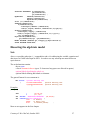
Direct assignment
Data may also be entered through replacement or assignment statements. Such statements
involve the use of a statement like
parametername(setdependency) = expression;
where the parameters on the left hand side must have been previously defined in a set, parameter
or table statement.
Examples
(Caldata.gms)
scalar a1;
scalars a2 /11/;
parameter
cc(j) , bc(j) /j2 22/;
a1=10;
a2=5;
cc(j)=bc(j)+10;
cc("j1")=1;
Courtesy of B.A. McCarl, October 2002
30
Notes
When a statement like cc(j)=bc(j)+10; is executed this is done for all elements in j so if j
had 100,000 elements this would define values for each and every one.
These assignments can be the sole entry of a data item or may redefine items.
If an item is redefined then it has the new value from then on and does not retain the
original data.
The example cc("j1")=1; shows how one addresses a single specific element not the
whole set, namely one puts the entry in quotes (single or double). This is further
discussed in the Sets chapter.
Calculations do not have to cover all set element cases of the parameters involved
(through partial set references as discussed in the Sets chapter). Set elements that are not
computed over retain their original values if defined or a zero if never defined by entry or
previous calculation.
A lot more on calculations appears in the Calculating chapter.
Algebraic nature of variable and equation specifications
When one moves to algebraic modeling the variable and equation declarations can have an added
element of set dependency as illustrated in our examples and reproduced below
POSITIVE VARIABLES
VARIABLES
EQUATIONS
x(j);
PROFIT
OBJective
constraint(i) ;
POSITIVE VARIABLES
EQUATIONS
P(commodities)
Qd(commodities)
Qs(commodities) ;
PDemand(commodities)
PSupply(commodities)
Equilibrium(commodities)
;
,
;
Such definitions indicate that these variables and equations are potentially defined for every
element of the defining set (also called the domain) thus x could exist for each and every element
in j. However the actual definition of variables does not occur until the .. equation specifications
are evaluated as discussed next. More on set dependent variable and equation definitions
appears in the Variables, Equations, Models and Solves chapter.
Algebra and model .. specifications
The equations and variables in a model are defined by the evaluation of the .. equation
specifications. The .. equations for our examples are
OBJective.. PROFIT=E=
SUM(J,c(J)*x(J)) ;
constraint(i).. SUM(J,a(i,J) *x(J)) =L= b(i);
Courtesy of B.A. McCarl, October 2002
31
Pdemand(commodities)..
P(commodities)=g=
intercepts("demand",commodities)
+sum(cc,slopes("demand",commodities,cc)*Qd(cc));
Psupply(commodities)..
intercepts("supply",commodities)
+sum(cc,slopes("supply",commodities,cc)* Qs(cc))
=g= P(commodities);
Equilibrium(commodities)..
Qs(commodities)=g= Qd(commodities);
Here GAMS will operate over all the elements in the sets in each term. For example, in the
OBJective equation GAMS will add up the term c(J)*x(J) for all set elements in j. Similarly, the
equation constraint(i) will define a separate constraint equation case for each element of i. Also
within the equation case associated with an element of i only the elements of a(i,j) associated
with that particular i will be included in the term SUM(J,a(i,J) *x(J)). Similarly, within the
second example equations of each type are included for each member of set commodities.
Notes
These examples show us moving away from the data specification that we were
employing in the GAMS the early GAMS examples in this chapter. In particular rather
than entering numbers in the model we are now entering data item names and associated
set dependency. This permits us to specify a model in a more generic fashion as will be
discussed in a later section of this tutorial on virtues of algebraic modeling.
The only variables that will be defined for a model are those that appear with nonzero
coefficient somewhere in at least one of the equations defined by the .. equations.
More on .. specifications appears within the Variables, Equations, Models and Solves
chapter.
Output differences
When set dependency is used in association with variables and equations and model then this
changes the character of a few of the output items. In particular, there are some changes in the
equation listing, variable listing, and solution reports for variables and equations.
Equation listing
The equation listing exhibits a few different characteristics in the face of set dependent variable
and equation declarations. In particular, the variables declared over sets are reported with a
display of their set dependency encased in parentheses. Also the equations declared over sets
have multiple cases listed under a particular equation name. An example is presented below in
the context of our core optimization example (optimize.gms) and shows three cases of the x
variable (those associated with the corn, wheat, and cotton set elements). It also shows that two
cases are present for the equation called constraint (land and labor).
---- OBJective
=E=
Courtesy of B.A. McCarl, October 2002
32
OBJective..
- 109*x(Corn) - 90*x(Wheat) - 115*x(Cotton) + PROFIT =E= 0 ; (LHS = 0)
---- constraint =L=
constraint(Land).. x(Corn) + x(Wheat) + x(Cotton) =L= 100 ; (LHS = 0)
constraint(Labor).. 6*x(Corn) + 4*x(Wheat) + 8*x(Cotton) =L= 500 ; (LHS = 0)
A portion of the equation listing from a more involved example ( model.gms) also reveals
additional differences. In the TCOSTEQ equation that we see the portrayal of coefficients
involved with several declared variables: 3 cases of Build, 6 cases of Shipsw, 6 cases of
Shipwm and 4 cases of Shipsm. The model.gms example also shows what happens there are
more cases of equation than the number of equation output items output by default as controlled
by the option Limrow (as discussed in the Standard Output chapter). In this case Limrow was set
to 2 but there were three cases of the equation named Capacity and GAMS indicates that one
case was skipped. If there had been 100, then 98 would have been skipped.
---- TCOSTEQ =E= TOTAL COST ACCOUNTING EQUATION
TCOSTEQ.. Tcost - 50*Build(A) - 60*Build(B) - 68*Build(C) - Shipsw(S1,A) - 2*Shipsw(S1,B)
- 8*Shipsw(S1,C) - 6*Shipsw(S2,A) - 3*Shipsw(S2,B) - Shipsw(S2,C) - 4*Shipwm(A,D1)
- 6*Shipwm(A,D2) - 3*Shipwm(B,D1) - 4*Shipwm(B,D2) - 5*Shipwm(C,D1) - 3*Shipwm(C,D2)
- 4*Shipsm(S1,D1) - 8*Shipsm(S1,D2) - 7*Shipsm(S2,D1) - 6*Shipsm(S2,D2) =E= 0 ;
(LHS = -4, INFES = 4 ***)
---- CAPACITY
CAPACITY(A)..
CAPACITY(B)..
=L= WAREHOUSE CAPACITY
- 999*Build(A) + Shipwm(A,D1) + Shipwm(A,D2) =L= 0 ; (LHS = 0)
- 60*Build(B) + Shipwm(B,D1) + Shipwm(B,D2) =L= 0 ; (LHS = 0)
REMAINING ENTRY SKIPPED
Variable list
The variable listing also exhibits a few different characteristics in the face of set dependent
variable and equation declarations. In particular, the variables declared over sets have multiple
cases listed under a particular variable name as do any involved sets. An example is presented
below in the context of our core optimization example (optimize.gms) and shows three cases of
the x variable (those associated with the corn, wheat, and cotton set elements). It also shows that
the variables use resources from two cases of the equation called constraint (land and labor).
---- x
x(Corn)
-109
1
6
x(Wheat)
-90
1
4
x(Cotton)
-115
1
8
(.LO, .L, .UP = 0, 0, +INF)
OBJective
constraint(Land)
constraint(Labor)
(.LO, .L, .UP = 0, 0, +INF)
OBJective
constraint(Land)
constraint(Labor)
(.LO, .L, .UP = 0, 0, +INF)
OBJective
constraint(Land)
constraint(Labor)
A portion of the variable listing from the more involved model.gms example shows GAMS
indicating four cases were skipped when Limcol was smaller than the number of cases on
hand(as discussed in the Standard Output Chapter).
Courtesy of B.A. McCarl, October 2002
33
---- Shipsw Amount Shipped To Warehouse
Shipsw(S1,A)
(.LO, .L, .UP = 0, 0, 1000)
-1
TCOSTEQ
1
SUPPLYEQ(S1)
-1
BALANCE(A)
Shipsw(S1,B)
(.LO, .L, .UP = 0, 0, 1000)
-2
TCOSTEQ
1
SUPPLYEQ(S1)
-1
BALANCE(B)
REMAINING 4 ENTRIES SKIPPED
Equation solution report
The equation solution LST also shows all existing cases grouped under each equation name
when set dependency is present as illustrated below in the context of our core optimization
example (optimize.gms).
---- EQU constraint
LOWER
LEVEL
Land
-INF
100.000
Labor
-INF
500.000
UPPER
100.000
500.000
MARGINAL
52.000
9.500
Variable solution report
The variable solution LST segment also shows all existing cases grouped under each variable
name when set dependency is present as illustrated below in the context of our core optimization
example (optalgebra.gms).
---- VAR x
LOWER
Corn
.
Wheat
.
Cotton
.
LEVEL
50.000
50.000
.
UPPER
+INF
+INF
+INF
MARGINAL
.
.
-13.000
Good modeling practices
Above I have covered the essential GAMS features one would employ in any modeling exercise.
However I have not done very good job of exploiting a major GAMS capability involved selfdocumentation. In any modeling exercise there are an infinite variety of choices that can be made
in naming the variables, equations, parameters, sets etc. and formatting their presentation in the
GMS instruction file. Across these choices that can be large differences in the degree of selfdocumentation within the GMS code. In particular, as explained in the chapter on Rules for Item
Names, Element names and Explanatory Text, one employ short names like x(j) as in
optalgebra.gms or longer names (up to 31 characters) for the variables like production(products).
I advocate use of longer names to enhance the readability of the document.
The GAMS also permits one to add comments, for example telling what is being done by
Courtesy of B.A. McCarl, October 2002
34
particular instructions or indicating data sources. This can be done by a number of means
including typing lines beginning with an * in column one or encasing longer comments between
a $ONTEXT and $OFFTEXT. GAMS elements for including comments are discussed in the
chapter entitled Including Comments.
I illustrate the longer name and comment capability along with improved spacing and line
formatting in the context of the model optalgebra.gms creating the new model
goodoptalgebra.gms. The two models use the same data and get the same answer only the item
names and formatting have been changed. In my judgment, the longer names substantially
contribute to self-documentation and make it easier to go back to use a model at a future time or
transfer a model to others for their use. More material on the formatting subject appears in the
Writing Models and Good Modeling Practices chapter.
Original version
optalgebra.gms
SET
j
/Corn,Wheat,Cotton/
i
/Land ,Labor/;
PARAMETER
c(j)
/ corn
109
,wheat
90 ,cotton
115/
b(i)
/land 100 ,labor 500/;
TABLE a(i,j)
corn
wheat cotton
land
1
1
1
labor
6
4
8
;
POSITIVE VARIABLES
x(j);
VARIABLES
PROFIT
;
EQUATIONS
OBJective
, constraint(i) ;
OBJective.. PROFIT=E=
SUM(J,(c(J))*x(J)) ;
constraint(i).. SUM(J,a(i,J) *x(J)) =L= b(i);
MODEL RESALLOC /ALL/;
SOLVE RESALLOC USING LP MAXIMIZING PROFIT;
Revised version with comments in blue
goodoptalgebra.gms
*well formatted algebraic version of model optalgebra.gms
SET
Products Items produced by firm
/Corn
in acres,
Wheat in acres ,
Cotton in acres/
Resources Resources limiting firm production
/Land
in acres,
Labor in hours/;
PARAMETER Netreturns(products) Net returns per unit produced
/corn 109 ,wheat 90 ,cotton 115/
Endowments(resources) Amount of each resource available
/land 100 ,labor 500/;
TABLE
Resourceusage(resources,products) Resource usage per unit produced
corn
wheat cotton
land
1
1
1
labor
6
4
8
;
POSITIVE VARIABLES
Production(products) Number of units produced;
VARIABLES
Profit
Total fir summed net returns ;
EQUATIONS
ProfitAcct
Profit accounting equation ,
Available(Resources) Resource availability limit;
$ontext
Courtesy of B.A. McCarl, October 2002
35
specify definition of profit
$offtext
ProfitAcct..
PROFIT
=E= SUM(products,netreturns(products)*production(products)) ;
$ontext
Limit available resources
Fix at exogenous levels
$offtext
available(resources)..
SUM(products,
resourceusage(resources,products) *production(products))
=L= endowments(resources);
MODEL RESALLOC /ALL/;
SOLVE RESALLOC USING LP MAXIMIZING PROFIT;
Structure of GAMS statements, programs and the ;
Now that I have been through the most essential basic elements of the GAMS syntax, I can
review the general format of GAMS statements and GMS files. A GAMS program is a collection
of statements in the GAMS language. A number of comments can be made about how the file
needs to be formatted
Statements must be ordered so that items are initially declared before they are used. If
they are used on the right hand side of a calculation (an = statement) they also must be
given data before use. If they are used in a model equation then they must be given data
before a Solve appears. This is enforced by GAMS indicating a lack of declaration and
numerical specification as a compilation error so one does not need to meticulously check
order of declaration, definition and use.1
Individual GAMS statements can be formatted in almost any style. Multiple lines may be
used for a statement, blank lines can be embedded, any number of spaces or tabs may be
inserted and multiple statements may be put on one line separated by a ;
Every GAMS statement should be terminated with a semicolon, as all the examples in
this book illustrate.
GAMS is not case sensitive, thus it is equivalent to type the command VARIABLE as
variable or the variable names XCOTTON as XcOttoN. However, there is case
sensitivity with respect to the way things are printed out with the first presentation being
the one used as discussed in the Rules for Ordering and Capitalization chapter.
The use of a named item (which in GAMS can be a set, parameter, scalar, table, acronym,
variable, equation, model or file) involves three steps:
Declaration where one announces the existence of a named item giving it a name.
Assignment giving it a specific value or replacing its value with the results of an
expression.
1
This a a number of the other points in this section are adapted from Richard E. Rosenthal's "A
GAMS Tutorial" that appeared in the GAMS Users Guide documents by Brooke et al.
Courtesy of B.A. McCarl, October 2002
36
Subsequent usage.
The item names, elements and explanatory text must follow certain rules as discussed in
the Rules for Item Names, Element names and Explanatory Text chapter.
Adding complexity
There are a few more topics meritorious of coverage in this tutorial that involve GAMS
capabilities to include conditionals, display data, do calculations incorporating optimal solution
information and solve a model more than once. Each is discussed below
Conditionals
Certainly when doing calculations and setting up models cases arise where one might wish to do
different things conditional upon data. In particular, one might wish to do a calculation like
z=x/y only if y is nonzero or one might wish to define demand equations only for cases where
demand exists. Incorporation of such considerations into GAMS program involves what's
known as the $conditional as extensively discussed in the Conditionals chapter. Below I present
several examples of this feature. Generally the expressions are of the form
term$logical condition
which says do something with term only if the logical condition is true where the $ can be read
as if it were the word if. Conditionals can appear in a number of contexts, as I will illustrate
below.
Conditionally execute an assignment
The condition
X$(y gt 0) = 10;
says set X=10 if the scalar y is greater than zero, while the condition
percentchange$(y ne 0)= 100*(x-y)/y;
says compute the item percentchange if y is not equal to zero.
For more on this class of conditionals see the discussion in the Conditionals chapter.
Conditionally add a term in sum or other set operation
The condition
z=sum(i$(y(i) gt 0),x(i));;
says include the term for set element i only if y(i) > 0, while
Courtesy of B.A. McCarl, October 2002
37
z=sum((i,j)$(sameas(i,j)),x(i,j));
says add the term corresponding to a pair of set elements i and j only if the set elements have the
same name (thus if the name of element i was Chicago then the j term would be included in the
sum only if the name of element j was Chicago).
For more on this class of conditionals see the discussion in the Conditionals chapter. For more
on Sameas also see the Conditionals chapter
Conditionally define an equation
The conditions
Eq1$(qq gt 0)..
xvar=e=3;
Eq2$(sum(I,q(i)) gt 0).. yvar=l=4;
Eq3(i)$(a(i) gt 0)..
ivar(i)=g= -a(i);
each cause an equation to exist in a model only if the condition is satisfied.
For more on this class of conditionals see the discussion in the Conditionals chapter.
Conditionally include a term in an equation
The conditions
..
Eq4
xvar+yvar$(qq gt 0)=e=3;
X=sum(I,q(i))$(qq gt 0)+4;
Q(i)=a(i)+1$(a(i) gt 0);
each cause the term in red to only be included in an expression (it is treated as zero otherwise)
only if the condition is satisfied.
For more on this class of conditionals see the discussion in the Conditionals chapter.
Displaying data
One may display any GAMS parameter, set, variable attribute, equation attribute or model
attribute as well as quoted text using the GAMS display statement. Generally the display is of
the format
DISPLAY ITEM1,ITEM2,ITEM3;
where the items are either
Quoted strings in single or double quotes such as
Courtesy of B.A. McCarl, October 2002
38
Display
'here
', "hello";
it is
Parameter or set names without any referencing to setdependency. Thus in Dispord.gms
while the parameter data is defined over 4 sets
parameter data(index1,index2,index3,index4);
I simply say
display data;
Variable, equation or model attributes with the item name and attribute desired specified
Display x.l, eq.m;
Multiple items can be listed in a display statement separated by commas.
Notes
Display will not print out items that are zero leaving blanks or skipping items where
entire rows or columns are zero.
GAMS displays can be enhanced in terms of form, and content in several ways as
discussed in the Report Writing Chapter. On option is to use the option command
OPTION ITEMNAME:DECIMAL:ROWitems:COLUMNitems
which will cause all subsequent displays of the named item to follow rules specified by
three numbers following the colons which are
DECIMAL
ROWitems
COLUMNitems
number of decimal places to be included
number of indices displayed within rows
number of indices displayed within columns
A display formatting sequence is introduced into the optimization example
(goodoptalgebra.gms) as follows:
option thisreport:2:1:2;
display thisreport;
which says use 2 decimal places and produce a display with 1 item in the rows and 2 in
the columns yielding
Land
Labor
Total
Available
Use by
Corn
Use by
Wheat
Marginal
Value
100.00
500.00
50.00
300.00
50.00
200.00
52.00
9.50
A display of the same item with option thisreport:4:2:1; yields
Courtesy of B.A. McCarl, October 2002
39
Land .Total
Land .Use by
Land .Marginal
Labor.Total
Labor.Use by
Labor.Marginal
Corn
Wheat
50.0000
50.0000
Available
Value
100.0000
52.0000
500.0000
300.0000
200.0000
9.5000
Report writing
GAMS permits one to do calculations using solution information to improve the information
content of the output. This exercise is commonly called report writing. Information relative to
the variable, equation and model solution is passed to GAMS from solvers. These data can be
used in report writing computations.
In GAMS the solution level for a variable is Variablename.L while it is Equationname.L for an
equation. The dual or shadow price information for an equation is addressed as Equationname.M
and the reduced cost for a variable is Equationname.M. The numerical values of these
parameters are generally undefined until a solve is performed and retains the value from the most
recent solve from then on. In the algebraic version of the equilibrium model (econequilalg.gms)
I introduce the following report writing sequence
set qitem /Demand, Supply, "Market Clearing"/;
set item /Quantity,Price/
parameter myreport(qitem,item,commodities);
myreport("Demand","Quantity",commodities)= Qd.l(commodities);
myreport("Supply","Quantity",commodities)= Qs.l(commodities);
myreport("Market Clearing","Price",commodities)= p.l(commodities);
display myreport;
which saves the supply and demand quantities along with the market clearing price. The
resultant report is generated with a display statement and is
----
39 PARAMETER myreport
Supply
.Quantity
Demand
.Quantity
Market Clearing.Price
Corn
Wheat
1.711
1.711
2.671
8.156
8.156
4.618
where I have color coded the originating statements and resultant output.
A report writing sequence is also introduced into the optimization example (goodoptalgebra.gms)
as follows
set item /Total,"Use by",Marginal/;
set qitem /Available,Corn,Wheat,Cotton,Value/;
parameter Thisreport(resources,item,qitem) Report on resources;
Thisreport(resources,"Total","Available")=endowments(resources);
Thisreport(resources,"Use by",qitem)=
sum(products$sameas(products,qitem),
resourceusage(resources,products) *production.l(products));
Courtesy of B.A. McCarl, October 2002
40
Thisreport(resources,"Marginal","Value")=
available.m(resources);
option thisreport:2:1:2;
display thisreport;
where both equation marginals (shadow prices) and variable levels are included in the report
writing calculations. This yields the report
Land
Labor
Total
Available
Use by
Corn
Use by
Wheat
Marginal
Value
100.00
500.00
50.00
300.00
50.00
200.00
52.00
9.50
where I have color coded the originating statements and resultant output.
The report wring topic is extensively discussed in the Report Writing chapter with a more
advanced discussion also appearing in the Output via Put Commands chapter.
Why use GAMS and algebraic modeling
Finally I feel it is beneficial to examine the attributes and difficulties with GAMS based
algebraic modeling. This is done under the following topics
Use of algebraic modeling
Context changes,
Expandability
Augmenting models
Aid with initial formulation and subsequent changes
Adding report writing
Self-Documenting Nature
Large Model Facilities
Automated Problem Handling
Model Library and widespread professional use
Use by Others
Ease of use with nonlinear, mixed integer, CGE and other problem forms
Interface with other packages
Use of algebraic modeling
GAMS permits one to express a formulation in general algebraic terms using symbolic
summation notation. This allows modelers to concisely state problems, largely independent of
the data and exact application context. Such formulations are inherently expandable, easily
subjected to context changes, and easily augmented as will be discussed just below.
However use of algebraic modeling can be a two edged sword GAMS algebraic requirements
and summation notation are difficult for some users. Some people will always desire to deal
with the exact problem context, not an abstract general formulation. This does lead to a strategy
Courtesy of B.A. McCarl, October 2002
41
most modelers use when employing GAMS modeling. Namely, GAMS exercises are usually
supported by small hand formulations that capture problem essence and serve as an aid in GAMS
model formulation.
Context changes
Consider the optimization example from above (goodoptalgebra.gms) which involved a farming
example. This can be rewritten to another context as follows (newcontext.gms)
SET
Products Items produced by firm
/Chairs , Tables , Dressers /
Resources Resources limiting firm production
/RawWood , Labor , WarehouseSpace/;
PARAMETER Netreturns(products) Net returns per unit produced
/Chairs 19 , Tables 50, Dressers 75/
Endowments(resources) Amount of each resource available
/RawWood 700 , Labor 1000 , WarehouseSpace 240/;
TABLE
Resourceusage(resources,products) Resource usage per unit produced
Chairs
Tables Dressers
RawWood
8
20
32
Labor
12
32
45
WarehouseSpace
4
12
10
;
POSITIVE VARIABLES
Production(products) Number of units produced;
VARIABLES
Profit
Total fir summed net returns ;
EQUATIONS
ProfitAcct
Profit accounting equation ,
Available(Resources) Resource availability limit;
ProfitAcct..
PROFIT
=E= SUM(products,netreturns(products)*production(products)) ;
available(resources)..
SUM(products,
resourceusage(resources,products) *production(products))
=L= endowments(resources);
MODEL RESALLOC /ALL/;
SOLVE RESALLOC USING LP MAXIMIZING PROFIT;
where only the lines in black changed not those in red relative to the farming example. So what?
The algebraic structure once built did not need to be altered and GAMS models can easily be
changed from one context to another.
Expandability
Consider the newcontext.gms optimization example from just above that made three products
from three resources. Two new products and two new resources can be added as follows
(expand.gms)
SET
Products Items produced by firm
/Chairs , Tables , Dressers, HeadBoards, Cabinets /
Resources Resources limiting firm production
/RawWood , Labor , WarehouseSpace , Hardware, ShopTime/;
PARAMETER Netreturns(products) Net returns per unit produced
/Chairs 19,Tables 50,Dressers 75,HeadBoards 28,Cabinets 25/
Endowments(resources) Amount of each resource available
/RawWood 700,Labor 1000,WarehouseSpace 240,Hardware 100, Shoptime 600/;
TABLE
Resourceusage(resources,products) Resource usage per unit produced
Chairs
Tables Dressers HeadBoards Cabinets
RawWood
8
20
32
22
15
Labor
12
32
45
12
18
WarehouseSpace
4
12
10
3
7
Hardware
1
1
3
0
2
Courtesy of B.A. McCarl, October 2002
42
Shoptime
POSITIVE VARIABLES
VARIABLES
EQUATIONS
6
8
Production(products)
Profit
ProfitAcct
Available(Resources)
30
5
12;
Number of units produced;
Total fir summed net returns ;
Profit accounting equation ,
Resource availability limit;
ProfitAcct..
PROFIT
=E= SUM(products,netreturns(products)*production(products)) ;
available(resources)..
SUM(products,
resourceusage(resources,products) *production(products))
=L= endowments(resources);
MODEL RESALLOC /ALL/;
SOLVE RESALLOC USING LP MAXIMIZING PROFIT;
where only the material in black was added with no alterations of that in red relative to the
newcontext.gms example. So what? The algebraic structure once built did not need to be altered
and GAMS models can easily be expanded from smaller to larger data sets. Such capabilities
constitute a major GAMS model development strategy. One can originally develop a model with
a small data set and fully debug it. Then later one can move to the full problem data set without
having to alter any of the algebraic structure but have confidence in the algebraic structure. This
is discussed further in the Small to Large: Aid in Development and Debugging chapter.
Augmentation
Consider the newcontext.gms optimization example from just and suppose we wish to augment
the model with constraints and variables reflecting the capability to rent or hire additional
resources subject to a maximum availability constraint. This is done in the following example
(augment.gms)
SET
Products Items produced by firm
/Chairs , Tables , Dressers /
Resources Resources limiting firm production
/RawWood , Labor , WarehouseSpace/
Hireterms Resource hiring terms
/Cost , Maxavailable /;
PARAMETER Netreturns(products) Net returns per unit produced
/Chairs 19 , Tables 50, Dressers 75/
Endowments(resources) Amount of each resource available
/RawWood 700 , Labor 1000 , WarehouseSpace 240/;
TABLE
Resourceusage(resources,products) Resource usage per unit produced
Chairs
Tables Dressers
RawWood
8
20
32
Labor
12
32
45
WarehouseSpace
4
12
10
;
Table
Hiredata(Resources,hireterms) Resource hiring data
Cost
Maxavailable
RawWood
3
200
Labor
12
120
WarehouseSpace
4
112;
POSITIVE VARIABLES
Production(products)
Number of units produced
HireResource(Resources) Resources hired;
VARIABLES
Profit
Total firm summed net returns ;
EQUATIONS
ProfitAcct
Profit accounting equation ,
Available(Resources)
Resource availability limit
Hirelimit(Resources)
Resource hiring limit;
ProfitAcct..
PROFIT
=E= SUM(products,netreturns(products)*production(products))
-SUM(resources,hiredata(resources,"cost")* HireResource(Resources))
available(resources)..
SUM(products,
Courtesy of B.A. McCarl, October 2002
;
43
resourceusage(resources,products) *production(products))
=L= endowments(resources) + HireResource(Resources);
Hirelimit(Resources)..
HireResource(Resources) =l= hiredata(resources,"maxavailable");
MODEL RESALLOC /ALL/;
SOLVE RESALLOC USING LP MAXIMIZING PROFIT;
where only the material in black was added with no alterations of that in red relative to the
newcontext.gms example. So what? The algebraic structure from the other study could be used
supplied the core of the new model with structural features added as needed. Such a capability
constitutes another major GAMS model development strategy.
One can adapt models from other studies customizing them for the problem at hand speeding up
the development process. In addition to adapting models from related studies done by the
modeler or the group in which the modeler works, there are number of other sources one may be
able to exploit to jumpstart a model development project. This is further discussed below.
Aid with initial formulation and subsequent changes
GAMS aids both in initially formulating and subsequently revising formulations. GAMS
facilitates specification and debugging of an initial formulation by allowing the modeler to begin
with a small data set, then after verifying correctness expand to a much broader context. For
example, one could initially specify a small transportation model with a few suppliers and
demanders. Then after that model is debugged one could expand the problem to encompass fifty
shipping origins and two hundred destinations without needing to change the algebraic model as
discussed in the Small to Large: Aide in Development and Debugging chapter and the
expandability section above.
GAMS also makes it easy to alter the model. Large models in programs like spreadsheets can be
difficult to modify. In a spreadsheet, I find it hard to add in a set of new constraints and
variables properly interjecting all the linkages and cannot figure out how to easily get a model
right with a few commodities then automatically expand the model scope to many commodities
and locations as illustrated in the expandability section above. On the other hand, GAMS allows
one to add model features much more simply. Generally, modelers do not try to make a
complete formulation the first time around. Rather one starts with a small formulation and then
adds structural features as needed adding features as illustrated in the augmentation section
above. GAMS also enforces consistent modeling, allowing models to be transferred between
problem contexts as shown above.
Adding report writing
Generally, default GAMS output for the model solution is not adequate for conveying solution
information to the modeler or associated decision-makers. One often does calculations using
solution information to improve information content of the GAMS output. This is elaborated
upon in the Report Writing chapter.
Self-documenting nature
Courtesy of B.A. McCarl, October 2002
44
One important GAMS feature its self-documenting nature. Modelers can use long variable,
equation and index names as well as comments, data definitions etc., allowing a readable and
fairly well documented problem description. Model structure, assumptions, and any calculation
procedures used in the report writing are documented as a byproduct of the modeling exercise in
a self-contained file. Comment statements can be inserted by placing an asterisk in column one,
followed by text identifying data sources or particular assumptions being used (i.e., in some of
the my models, comments identify data source publication and page). Under such circumstances
GAMS allows either the original author or others to alter the model structure and update data.
Consider for example the following example. Can you figure out what context the example is
from?
LABOR(Farm)..
PLOWLAB(Farm) * PLOW(Farm)
+ SUM( crop, PLNTLAB(Farm,Crop) *PLANT(Farm,Crop)
+ HARVLAB(Farm,Crop) * HARVEST(Farm,Crop) )
=L= LABORAVAIL(Farm);
Large model facilities
GAMS is not the tool of choice for small, infrequently solved problems. In such cases, the
generality of the presentation may not be worth the effort, and spreadsheet or other formulations
are probably quicker and easier to deal with. GAMS is best employed for medium or large sized
models (more than 100 rows and/or columns) and can handle large problems as the table of a few
or my application model sizes below indicates.
MODELS
VARIABLES
10 REGION ASM
9860
ASM
30146
SOIL ASM
41574
GLOBAL ASM(sto)
EQUATIONS
NOTES ON
IMPLEMENTATION
811
412 crop budgets
129 livestock
45423 lines 2.9Mb
2844
1662 crop budgets
838 livestock budgets
60469 lines 8.3Mb
2935
123087 lines 33.6Mb
305605
14556
120991 lines 43.5Mb
FASOM
26012
1774
141697 lines 35.3Mb
HUMUS
429364
236234
41444 lines 123.1Mb
12161
5655
7858 lines 6.1Mb
EDWARD
The gains to using GAMS rise with problem size and complexity of the model use exercise
study. When a modeler deals with large problems, the GAMS algebraic statement is probably
the only thing that is thoroughly understood. Often the numerical formulation has grown out of
control.
Courtesy of B.A. McCarl, October 2002
45
Automated problem handling and portability
Many of the tasks that would traditionally have required a computer programmer are automated.
As such, GAMS automatically does coefficient calculation; checks the formulation for obvious
flaws; chooses the solver; formats the programming problem to meet the exact requirements of
the solver; causes the solver to execute the job; saves and submits the advanced basis when doing
related solutions; and permits usage of the solution for report writing. Also GAMS verifies the
correctness of the algebraic model statements and allows empirical verification using programs
like GAMSCHK.
Furthermore, GAMS code is portable between computers. GAMS has been implemented on
machines ranging from PCs to UNIX/LINUX workstations to CRAY super computers. Exactly
the same code runs on all of these computer systems.
Switching solvers is simple requiring changing a solver option statement or changing from using
LP to using NLP as discussed in the Variables, Equations, Models and Solves chapter. Links to
spreadsheets have also been developed as discussed in the Links to Other Programs Including
Spreadsheets chapter.
Model library and widespread professional use
Today GAMS has become the de facto standard for optimization modeling in many fields.
Modelers may be able to adapt models or gain insights from others. Some sources of models
from which model features can be adapted include:
Models from experienced users that address similar problems that are closely related in
concept or structure and can be adapted.
Models associated with textbooks. For example, my book with Spreen contains many
examples. The book and the examples are available through my Web page
agecon.tamu.edu\faculty\mccarl
Models are available through the GAMS library which is directly included in the IDE.
These cover many different settings.
References from the GAMS web pages http://www.gams.com/, http://www.gams.de/ , or
http://gamsworld.org/.
Each of these resources along with others are discussed in the chapter called Learning Resources:
Model Library, Web Sites, Documentation.
Use by Others
Modeling personnel are often rare. For example, in international development contexts, detailed
GAMS applications have been set-up by modeling experts but subsequently, the model is utilized
by policy-makers with minimal, if any, assistance from the modeling experts. Often, given
Courtesy of B.A. McCarl, October 2002
46
proper internal documentation and a few instructions, clerical labor and nontechnical problem
analysts can handle an analysis.
Ease of use with NLP, MIP, CGE and other problem forms
GAMS handles a variety of different problem types and has become one of principal languages
for computable general equilibrium modeling, agricultural economic modeling and oil refinery
modeling. It is also one of the principal platforms for experimentation with developing fields
like mixed integer nonlinear programming models and global optimization models. GAMS
Corporation is continually engaged in an effort to provide the most recent available solver
software. This likely implies that GAMS users will have available the most recent developments
in solver software and libraries of application test problems in emerging fields.
Interface with other packages
While not as well developed as I would like, GAMS does have procedures to interface with other
programs like spreadsheets, databases, custom control programs, and Visual basic procedures
among others. These interfaces are discussed in the chapter entitled to Links to Other Programs
including Spreadsheets.
Alphabetic list of features
.. specifications
.. specifications
Algebra
Algebraic modeling
Alias
Augmentation
Automated problem handling
Command line GAMS
Compilation errors
Conditionals
Context changes
Cross reference map
Data entry
Display
Echo print
Economic equilibrium
Equation listing
Equation listing
Equation solution report
Equation solution report
Equations
Equations
Tutorial coverage
Algebraic content, tutorial coverage
Tutorial coverage
GAMS exploitation of algebraic modeling - tutorial
coverage
Tutorial coverage
Expanding a core model - tutorial coverage
GAMS capabilities
Tutorial coverage
Tutorial coverage
Tutorial coverage
Changing model domain of applicability -tutorial coverage
Tutorial coverage
Tutorial coverage
Tutorial coverage
Tutorial coverage
Tutorial example
Tutorial coverage
Algebra use effects on, tutorial coverage
Tutorial coverage
Algebra use effects on, tutorial coverage
Algebraic content, tutorial coverage
Tutorial coverage
Courtesy of B.A. McCarl, October 2002
47
Execution output
Expandability
GAMSIDE approach
Generation listing
Good modeling practices
.L
Large model facilities
Library
Model
Model library
Model statistics
Nonlinear equation system
Optimization problem
Parameters
Portability
Report writing
Running a job
Scalars
Self-documenting nature
Sets
Solution Summary
Solve
Solver report
Structure of GAMS statements
Sums
Symbol list
Tables
Use by Others
Variable listing
Variable listing
Variable solution report
Variable solution report
Variables
Variables
Tutorial coverage
Small to large modeling - tutorial coverage
Tutorial coverage
Tutorial coverage
Tutorial coverage
Tutorial coverage
Tutorial coverage
Tutorial coverage
Tutorial coverage
Tutorial coverage
Tutorial coverage
Tutorial example
Tutorial example
Tutorial coverage
Platform independence
Tutorial coverage
Tutorial coverage
Tutorial coverage
Tutorial coverage
Tutorial coverage
Tutorial coverage
Tutorial coverage
Tutorial coverage
Tutorial coverage
Tutorial coverage
Tutorial coverage
Tutorial coverage
Tutorial coverage
Tutorial coverage
Algebra use effects on, tutorial coverage
Tutorial coverage
Algebra use effects on, tutorial coverage
Tutorial coverage
Algebraic content, tutorial coverage
Courtesy of B.A. McCarl, October 2002
48