Download User Manual

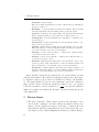
Institute of Systems and Robotics
University of Coimbra
EasyCamCalib User Manual
Version 1.1
August 24, 2011
1
Contents
Contents
2
1 Introduction
1.1 What is EasyCamCalib? . . . . . . . . . . . . . . . . . . . . . .
1.2 Basics of Single Image Calibration . . . . . . . . . . . . . . . .
1.3 Capturing Calibration Images . . . . . . . . . . . . . . . . . . .
3
3
3
4
2 Using EasyCamCalib
2.1 User Interface . . .
2.2 File Menu . . . . .
2.3 Edit Menu . . . . .
2.4 Tools Menu . . . .
2.5 Refinement . . . .
.
.
.
.
.
.
.
.
.
.
.
.
.
.
.
.
.
.
.
.
.
.
.
.
.
.
.
.
.
.
.
.
.
.
.
3 Calibration from a Single Image
.
.
.
.
.
.
.
.
.
.
.
.
.
.
.
.
.
.
.
.
.
.
.
.
.
.
.
.
.
.
.
.
.
.
.
.
.
.
.
.
.
.
.
.
.
.
.
.
.
.
.
.
.
.
.
.
.
.
.
.
.
.
.
.
.
.
.
.
.
.
.
.
.
.
.
.
.
.
.
.
.
.
.
.
.
.
.
.
.
.
6
6
6
8
8
13
13
4 Analysing the Calibration Data
15
4.1 EasyCamCalib output . . . . . . . . . . . . . . . . . . . . . . . 15
5 Known Issues
16
Bibliography
17
2
1
Introduction
1.1
What is EasyCamCalib?
The purpose of EasyCamCalib is to calibrate a camera with radial distortion
from a single image of a planar chessboard pattern. The application aims to
automatically calibrate a camera from an image (or a set of images), requiring minimal user intervention. The original goal of this application was to
calibrate an endoscope (high radial distortion) using a single image captured
by a surgeon on the operating room, but the methods are generalized to any
camera that presents moderate to high levels of radial distortion. Although
the algorithm is designed to provide accurate calibration using a single image,
the accuracy and robustness is increased when using more than one image.
1.2
Basics of Single Image Calibration
The EasyCamCalib toolbox is built upon the recent work of Barreto et al. [1],
where the authors are able to calibrate a camera presenting radial distortion
using a single image of a planar chessboard pattern. The radial distortion is
modeled using the so called division model [2] and the method provides a closed
form estimation of the intrinsic parameters and distortion coefficient. The
fact that the distortion follows a known model provides additional geometric
cues for achieving calibration from a single image. For further details on the
calibration algorithm please refer to [1].
The toolbox provides an interface that facilitates the calibration of a camera from a single image. The calibration is performed as follows:
• Boundary Detection (in the case of endoscopic or fish-eye lenses).
The boundary between the meaningful region of the arthroscopic image
and the background is defined. The boundary information is used to
later restrict the automatic corner detection of the chessboard pattern.
• Automatic Corner Detection. The image is searched for plausible
corners, which are referenced in the chessboard reference frame. This
detection is based in the entropy of the angles and uses geometric metrics
to validate and count the corners. Therefore, the automatic corner detection is sensitive to illumination conditions and view angle (as referred
in section 1.3).
3
1. Introduction
• Initial Calibration. With the automatic corners detected, a first calibration is estimated using [1]. This calibration will be referred as the
Initial Calibration.
• New Points Generation. Using the initial calibration estimation,
points are generated in the image plane and matched to squares of the
calibration grid. Note that, for lenses with strong radial distortion,
points generated in the periphery of the image tend to be inaccurate.
In this case you might need to use the manual selection tool to remove
undesired generated points.
• Final Calibration. With the new generated points the calibration
parameters are recomputed, providing what we will call from now on
the Final Calibration.
• Calibration Refinement. The calibration parameters are refined using a non linear optimization over the re-projection error. This is the
final result of the calibration and will be referred from now on as the
Optimal Calibration.
1.3
Capturing Calibration Images
For EasyCamCalib to be able to calibrate the camera from a single image, the
following requirements must be fulfilled:
Figure 1: Examples of bad calibration images. On the left we can see an image
in a fronto-parallel configuration. On the right we can see a highly slanted
calibration image. Both these images fail to calibrate automatically (you can
still use the slanted one to calibrate, but you will have to manually select some
of the input points).
4
1.3. Capturing Calibration Images
Figure 2: Examples of good calibration images
• The angle between the optical axis and the normal to the calibration
plane should be higher than 15o , i.e. you must avoid fronto-parallel
configurations (angle=0o ) in order to have a good decoupling between ξ
and the focal distance [1]. You also must avoid highly slanted views to
avoid bad automatic corner detections. Figures 1 and 2 illustrate some
good and bad calibration images examples.
• The number of squares present in the image must be enough to calibrate
from a single view. The image should contain at least 16 corners1 .
Note that the more points you provide to the algorithm, the better the
projection model will be estimated.
• The calibration grid must be in the central part of the image. An optimal
situation is when all the image is filled with the calibration grid. If
you cannot take calibration images in this conditions try to put the
1
This is not the minimum number of corners required to calibrate an image from a single
view
5
2. Using EasyCamCalib
calibration grid over a non-textured material (like a black fabric) to
avoid bad automatic corner detections.
One of the few limitations of the software comes from the automatic corner
detection used to initialize the calibration. If the calibration image does not
fulfil the above requirements there is a good chance that the calibration will
fail due to bad detected initial corners.
2
Using EasyCamCalib
To use EasyCamCalib, the easiest way is to add the Interfaces folder you
downloaded to the matlab path. This will only input some GUI executables
to your path. All the functions needed by EasyCamCalib are loaded locally so
your matlab path don’t get filled with unnecessary files. Currently the toolbox
needs the Matlab optimization toolbox. So, to start the software, simply call
“EasyCamCalib” from the matlab prompt.
2.1
User Interface
When you call EasyCamCalib from the matlab prompt you will find a GUI
similar to the one of figure 3. The UI have also a menu bar that will be
addressed bellow.
2.2
File Menu
Start
Start the calibration using the files in the calibration list. This menu has the
same function as the button 5 of Figure3.
Save Data
Save the calibration data in a .mat file that can be loaded later. Note that
during execution, as a fail-safe, EasyCamCalib saves intermediary results in
temp/CalibData temp.mat.
Save to txt
Save the intrinsic calibration parameters in .txt file. The parameters are saved
in the following order:
6
2.2. File Menu
10
8
12
7
9
11
13
1
6
2
3
4
5
Figure 3: Main EasyCamCalib window.
1. Browser list box. All the calibration images are chosen from this list box.
2. Calibration list. All the images you want
to use for calibration are listed here.
3. Preview window. As you click in the
browse list box or the calibration list box
a small preview off the image is presented
here.
4. Mean reprojection errors of the calibrated
images. The value in bold represents the
mean re-projection error of the current selected image.
5. Start calibrating the images of the calibration list.
8. Estimated extrinsic calibration parameters (relative pose between the camera
and the plane).
9. After the calibration is over, switch to the
calibration parameters you want to display.
10. Main visualization window. All the visual
results are presented here.
11. Angle of the camera relatively to the calibration plane and distance from the plane
origin to the optical center of the camera.
6. Options Button.
12. Visualization buttons. Read the tooltips
while using the toolbox for more information.
7. Estimated intrinsic calibration parameters.
13. Return to the calibration image selection
stage to perform a new calibration
7
2. Using EasyCamCalib
1. Coupled parameter between the focal distance and distortion coefficient
η = √f . This parameter is estimated during the linear calibration in
−ξ
[1].
2. Distortion coefficient according to the first order division model [2, 3].
3. Aspect Ratio.
4. Skew angle.
5. Principal point x-coordinate.
6. Principal point y-coordinate.
7. Focal distance.
The remaining values refer to the case of wide angle lenses where there is a
circular boundary limiting the meaningful region of the image.
Load Data
Load a previously saved .mat file.
2.3
Edit Menu
Options
Open the option UI of Figure4:
2.4
Tools Menu
Modify Points
Manually add or remove points from the calibration pattern. When you use
this tool all the images in the calibration list will pop-up consecutively, enabling you to add or remove any points to the calibration process. Here are
the commands you can use with this tool:
• Left Click - select the nearest corner for insertion and input the coordinates in the matlab prompt. Note that, although the coordinates
in the calibration plane are referenced in millimetres, when inputting
coordinates you have to input them in integer units (the origin corner is
set to [0,0], the next is [1,0], and so on...).
8
2.4. Tools Menu
1
2
5
6
3
7
4
Figure 4: Options window.
1. Define the calibration chessboard grid
size in millimetres. The grid is assumed
to be square.
2. Automatically set the same reference
frame in the calibration pattern across
multiple images. To be able to use this
feature the calibration images must fulfill
three requirements:
• The calibration grid must have
two diagonally consecutive white
squares painted with different colors.
• The colors of the marks should be
very distinctive in the HSV color
space. The colors tested usually
present both high Value and Saturation and a different value of Hue.
One good example is using light
blue and purple as marks colors.
• The marks should be nearby the
center of the image (if the image
has high distortion).
3. Setting this option will enable the calibration parameters non-linear optimization over all the images without needing
to run it manually from the menu.
4. Defines the image source.
If Endoscopic/FishEye Lens is selected, EasyCamCalib assumes that there is a wide
angle lens with high radial distortion and
will try to fit an ellipse to the boundary
contour of the meaningful region of the
image. If Normal Lens is selected the lens
is assumed to have moderate distortion.
5. Abort the whole calibration process in
case an image fails the calibration.
6. Automatically remove the images where
the process fails, leaving only the good
images for the calibration.
7. Save the defined options and quit to the
main UI.
9
2. Using EasyCamCalib
• Right Click - select the nearest point for removal. The point gets
surrounded by a yellow square.
• Middle Click - define a box (with two middle clicks) that select points
for removal.
• p - show/hide point coordinates.
• space - get to the next image.
• q - finish the manual selection here. The modifications you have done
so far are kept, the rest of the images stays untouched.
• s - set the size of the window where we will search for corners when
clicking in the image for inputting points.
• g - try to generate more interest points from the ones already existent.
Use carefully and always save your changes before attempting this.
Define Origins
Manually set the reference frame of the calibration plane for each image. You
define the origin with the Left Mouse click and the x direction with the Right
Mouse button. After you are done with one image press space to get to the
next image or press q to exit without further changes. It is very important
that you keep a constant reference frame across all calibration images. This
reference frame will be used to compute the extrinsic parameters (transform
from the image plane to the calibration grid).
Correct Radial Distortion
This tools aims at checking the projection model and distortion parameter(s)
estimation. When you correct the radial distortion, if the model is accurately
estimated, straight lines in the 3D world will be projected as straight lines
in the image plane. To use the UI of Figure5 simply select a calibration file
previously saved from the left list box, and the image you want to correct
from the right list box (a small preview will appear on the right.). Then hit
the start button. In the case of wide angle lenses where the radial distortion
is high, select the Arthroscope image source and input a desired undistorted
image size in pixels.
10
2.4. Tools Menu
Figure 5: Radial distortion correction UI.
(a) Original image.
(b) Corrected image.
Figure 6: Result of the radial distortion correction.
Figure 7: Homography checker UI.
11
2. Using EasyCamCalib
(a) Image 1.
(b) Image 2.
(c) Image 2 generated from
image 1 trough homography.
Figure 8: Result of the homography test.
Homography Checker
This tools checks the consistency of the extrinsic parameters through a visual
homography test. The UI of Figure7 is presented to the user, which has to
load a calibration file and select two images for the test.
After the user hits the start button, a new image 2 will be generated
though homography from image 1. This homography is computed using the
extrinsic parameters of the views and according to [3]. Figure7 shows the
result of the test in a wide angle lens (4mm arthroscope).
Note that this test only makes sense if all the images in the dataset generated a different calibration (see the 1st/2nd Order Refinement 1 by 1 presented
bellow). If you do this test on a dataset where all images were optimized together, since the non-linear optimization also optimizes the transforms, you
will be biasing the results
Compare with Bouguet
This tool launches the Bouguet [4] calibration toolbox over the current data
and compares the results with the EasyCamCalib estimations. Note that
the distortion profile curve has to be converted from the division model [2]
(used by EasyCamCalib) to the Brown’s model [5] used in the Bouguet’s
toolbox, which can introduce some error in the distortion parameters. Also
be aware that to do a fair comparison you have to use more than 10 images
and optimize the EasyCamCalib results using all the data (see 1st/2nd Order
Refinement bellow) before running the tool. In this comparison only two
distortion parameters are used in the Bouguet’s calibration estimation and
the tangential distortion is ignored. Also, both aspect-ratio and skew angle
are fixed to 1 and 0 respectively.
12
2.5. Refinement
2.5
Refinement
1st Order Refinement
Perform a non-linear optimization over all the input images assuming the
first order division model for radial distortion. Both intrinsics and extrinsic
parameters of all images are optimized together over the re-projection error of
the pixels. The Levenberg–Marquardt algorithm is used as the minimization
solution.
2nd Order Refinement
Perform a non-linear optimization over all the input images assuming the
second order division model for radial distortion. Both intrinsics and extrinsic
parameters of all images are optimized together over the re-projection error of
the pixels. The Levenberg–Marquardt algorithm is used as the minimization
solution.
1st Order Refinement 1 by 1
Perform a non-linear optimization over the input images independently assuming the first order division model for radial distortion. Both intrinsics
and extrinsics parameters of each images are optimized independently over
the re-projection error of the pixels. This means that in the end you will get
as many optimized calibrations as the number of images in the dataset. The
Levenberg–Marquardt algorithm is used as the minimization solution.
2nd Order Refinement 1 by 1
Perform a non-linear optimization over the input images independently assuming the second order division model for radial distortion. Both intrinsics
and extrinsics parameters of each images are optimized independently over
the re-projection error of the pixels. This means that in the end you will
get as many optimized calibrations as the number of images in the dataset.
Once again, the Levenberg–Marquardt algorithm is used as the minimization
solution.
3
Calibration from a Single Image
This is the quick guide to easily calibrate a camera from a single image. You
can start by choosing the image for the calibration from your dataset using
13
3. Calibration from a Single Image
the listbox of Figure9a. You can also navigate through your file system using
the path selector above.
The next step is to configure the calibration using the Options menu or
the button above the S tart button. The window of Figure9b will appear and
you will be able to define some options.
Specify grid size in millimeters
Endoscopic/Fisheye Lens
Normal Lens
(a) Choosing the calibration image from the(b) Configuring the calibration through the
list box.
options editor.
Figure 9: Calibrating from a single image - Step 1.
After the calibration customization you can hit the green Start button
and a confirmation dialogue will appear (Figure10a). After confirming the
calibration setup, hit the Proceed button to start the calibration.
After a while the first step of the calibration is completed. At this time
you can check the grid points used in the linear estimator and do small adjusts
using the Modify Points tool, as shown in Figure10b.
(a) Checking up the calibration setup.
(b) Adding/Removing points using the manual tool.
Figure 10: Calibrating from a single image - Step 2.
14
After making sure that no wrong input points are being used in the calibration, you can proceed to the non-linear optimizer. Use the Refinement
menu to choose the appropriate optimizer (Figure11a).
In the end you will finish with a complete calibration from a single image.
Check the results as indicated in Figure11b. After that you can return to the
first step using the Return button, or you can analyse the data as shown later.
(a) Running the non-linear optimizer.
(b) Final result of the calibration.
Figure 11: Calibrating from a single image - Step 3.
4
Analysing the Calibration Data
After a successful calibration, or any time you load a calibration file, the EasyCamCalib toolbox allows to visually inspect the data and check the parameters
estimation accuracy. With the provided tools you can see the re-projection
errors of each image, inspect the input points, the parameters change across
calibrations, the 3D transform between the calibration plane and the camera,
etc.
Further instruction about the advanced use of the toolbox can be found
in the tutorial video.
4.1
EasyCamCalib output
All the calibration data is stored in a MATLAB structure that is composed
by the following fields:
• ImageData
– ImageRGB - RGB image.
15
5. Known Issues
– ImageGrey - Grayscale image.
– Info - Some additional information about the calibration image, including the
grid size, resolution, etc.
– Hand2Opto - if any OptoTracker information is available, this 4x4 matrix
holds the transformation from the Hand (camera) to the Optotracker.
– Boundary - if the image was acquired with a wide angle lens, this field holds
all the boundary information (conic parameters, boundary points, etc.).
– PosImageAuto - Point automatically detected (in image coordinates) for the
Initial Calibration.
– PosPlaneAuto - Points automatically detected (in calibration plane coordinates) for the Initial Calibration.
– InitCalib - Initial calibration using only the automatically detected points.
Inside this structure, besides the intrinsic/extrinsic and distortion parameter,
you can also find the re-projection error information.
– PosImage - Corners detected in image coordinates after joining automatic
corners and new generated corners.
– PosPlane - Corners detected in plane coordinates after joining automatic corners and new generated corners.
– FinalCalib - Final calibration using all the corners (automatic corners + new
generated points). Inside this structure, besides the intrinsic/extrinsic and
distortion parameter, you can find the re-projection error information.
– OptimCalib - Optimal calibration after using the non-linear optimizer over
FinalCalib. Inside this structure, besides the intrinsic/extrinsic and distortion
parameter, you can also find the reprojection error information.
Inside InitCalib, FinalCalib and OptimCalib you can find all the relevant
calibration information. The calibration parameters (aspect ratio, skew angle,
focal distance and projection center) are identified according to the literature
[3]. The transformation T gives you the transform between the calibration
plane and the camera. Besides the parameters defined before, you can find
a distortion parameter ξ and a parameter η = √f , as well as the intrinsics
−ξ
matrix K (computed as usual in the literature [3]) and a matrix Kη used in
other applications.
5
Known Issues
• The major drawback of this software resides in the automatic corner
detection and counting for the first calibration parameters linear estimation. As the application targets a wide range of cameras and lens
with different distortions, this task is far from being trivial. The software must be able to handle illumination variations, resolution changes,
16
Bibliography
different sizes of the squares in the image, different amount and effects of
distortion, background clutter other than the calibration grid, different
shapes of the grid squares (as the perspective/distortion changes), etc.
Therefore, at this stage, the software is not yet completely automatic.
You will find yourself using the Modify Points tool quite often. This
issue will be addressed in the next releases.
• While analysing the calibration data you are able to change the viewpoint in the extrinsic parameters visualizer. For some reason the UI
has a bug that allows the user to change the viewpoint in all the other
figures of the UI. When this happens, simply change the image you are
analysing (clicking in a different item of the list box) and the axis will
go back to normal.
• It is possible that, if some input points are misplaced, the New Points
Generation step starves your system memory while generating an infinite number of points. When this happens you have to restart the
application.
Bibliography
[1] J. Barreto, J. Roquette, P. Sturm, and F. Fonseca, “Automatic
camera calibration applied to medical endoscopy,” in Proceedings of the
20th British Machine Vision Conference, London, UK, 2009. [Online].
Available: http://perception.inrialpes.fr/Publications/2009/BRSF09
[2] A. Fitzgibbon, “Simultaneous linear estimation of multiple view geometry
and lens distortion,” in Computer Vision and Pattern Recognition, 2001.
CVPR 2001. Proceedings of the 2001 IEEE Computer Society Conference
on, vol. 1, 2001, pp. I–125 – I–132 vol.1.
[3] Y. Ma, S. Soatto, J. Kosecka, and S. S. Sastry, An Invitation to 3-D Vision:
From Images to Geometric Models. SpringerVerlag, 2003.
[4] J.-Y. Bouguet. Camera Calibration Toolbox for Matlab. [Online]. Available: http://www.vision.caltech.edu/bouguetj/calib doc/index.html#ref
[5] D. C. Brown, “Decentering Distortion of Lenses,” Photometric Engineering, vol. 32, no. 3, pp. 444–462, 1966.
17