Download Week 9: Phylogeny, paleontology, and practical

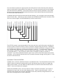
G563 Quantitative Paleontology
Department of Geological Sciences | P. David Polly
Week 9: Phylogeny, paleontology, and practical applications
Phylogenetic software
For this lab you will need to download and install the Mesquite, PHYLIP, and Phylogenetics for
Mathematica packages:
http://mesquiteproject.org/mesquite/mesquite.html
http://evolution.genetics.washington.edu/phylip.html
http://mypage.iu.edu/~pdpolly/Software.html
M esquite. Mesquite has tools for creating and modifying phylogenetic data matrices, as well as
tools for displaying trees and doing certain kinds of analysis on phylogenetic data. It does not,
however, do an exhaustive parsimony analysis. Mesquite’s documentation can be found by opening
the file “documentation.html” in your web browser.
PHYLIP. PHYLIP (Phylogenetic Inference Package) has modules for estimating phylogenetic trees
from data and for displaying the trees. We will use the Pars module, which calculates a parsimony
tree from multistate data, and the Consense module, which calculates a consensus tree (average)
when more than one tree is found by Pars. We will also use the ContML module, which calculates a
maximum likelihood tree from continuous data. PHYLIP’s documentation can be found in the folder
“docs” where you stored the PHYLIP package on your computer.
Phylogenetics for M athem atica. An add-in package for Mathematica that performs several
simple tree-related tasks, such as reading in a Newick format tree file, drawing trees, rerooting them,
simulating data on the trees, reconstructing ancestral nodes from the trees, and doing independent
contrasts. It also helps prepare data for export to PHYLIP. For this course, we will only use the tree
reading and drawing functions.
Running PHYLIP
Documentation. read the following pages in the PHYLIP documentation. Start by opening the help
file Main.html into your web browswer. Read it, then read the following:
discrete characters
Pars
Penny
Consense
I’ve uploaded two example data files to the website. One is made of up discrete characters from
selected credonts (mammalian carnivores from the Paleogene) from Polly (1996). (the dataset on
1
Oncourse is not identical to the one in the paper; some errors have been corrected, including
removal of a redundant character). The other is made up of quantitative traits describing the shape
of molars in marmots (big ground squirrels from the Neogene) from Polly (2003). You can use these
to get used to the program.
Polly, P. D. 1996 The skeleton of Gazinocyon vulpeculus gen et comb nov and the cladistic
relationships of Hyaenodontidae (Eutheria, Mammalia). Journal of Vertebrate Paleontology
16, 303-319.
Polly, P. D. 2003 Paleophylogeography: The tempo of geographic differentiation in marmots
(Marmota). Journal of Mammalogy 84, 369-384.
Both files are in the PHYLIP format, which is described in Felsenstein’s documentation. Basically the
format consists of a first line with two numbers, number of taxa and number of characters, followed
by lines that begin with a short taxon name followed by the character data.
The easiest way to run PHYLIP is to save the file you are working with in the folder with the PHYLIP
programs. Name the file “infile”. Note that Windows often adds an extension (such as .txt) that may
be hidden depending on your folder settings. PHYLIP saves output data in the files OUTFILE and
OUTTREE. The latter can be renamed with a “.tre” extension and opened in TreeView.
Parsimony Analysis
The PARS and PENNY programs do parsimony analysis. PARS handles characters with more states
than just 0 and 1. PENNY is more efficient than PARS for some data sets.
To run a parsimony analysis on the data in the file “INFILE” double click on PARS to start the
program. You are first faced with several options: type the letter in the left column to change the
associated option. You probably want to change the J option to randomize the input order (the
search sometimes is influenced by input order), you might also want to change option O (outgroup).
For the creodont data, set the outgroup to taxon 1 (which is a dummy outgroup taxon coded with all
ancestral character states).
Note that characters are considered to be unordered in PARS, which means that only one tree step is
required for a character to change from 0 to 1, 0 to 2, 0 to 3, 1 to 3, etc. This makes sense in many
cases if you don’t know the order of transition, but in other cases it may not make sense (e.g., digit
reduction might reasonably be assumed to go from 5 to 4 to 3 to 2 to 1 and not jump straight from 5
to 1).
When you are satisfied with your options, type Y to start the analysis. Progress reports will be printed
on the screen. When the program is finished, open OUTFILE in a text editor to see the results. The
creodont dataset yields 12 equally parsimonious trees, each with 114 steps.
The OUTTREE file can be viewed in Mesquite (it’s easiest to change the extension to .tre first and you
M UST remove the carriage returns from within each tree so that each one is on a separate line AND
remove the last number before the semicolon and its two square brackets). Open the file and
choose “Phylip (trees)” as the type when prompted to do so. You can see all 12 trees in Mesquite by
clicking on the View Trees icon and then paging through the trees with the arrow button at the top of
the screen. The first tree looks like this:
2
You can also view trees one at a time in Mathematica. Load the Phylogenetics package:
<<PollyPhylogenetics`
Then copy and paste the tree of interest into a file of its own. For example:
(Didelphodu:1.00,(((((Sinopa:1.79,((((Hyaenodon:1.87,notPterodo:2.20):7.24,Propterodo:1.23):8.14,
Eurotheriu:2.47):5.22,Gazinocyon:0.88):8.25):9.85,Prototomus:0.36):6.80,((Thinocyon:2.10,Prolimn
ocy:1.67):4.78,(((Hyainailou:4.00,Pterodon:1.25):7.67,Dissopsali:2.17):4.93,Arfia:3.19):8.26):6.05):
6.08,Proviverra:1.00):1.29,Cimolestes:1.00):1.29,Outgroup:0.00);
Then read in the tree:
tree = ReadNewick[‘tree1.tre’];
And plot the tree:
DrawNewickTree[tree]
Didelphodu
Sinopa
Node 5
Node 4
Node 3
Node 0
Node 2
Node 10
NodeHyainailou
14
Node 13 Pterodon
Node 12Dissopsali
Arfia
Proviverra
Cimolestes
Outgroup
10
Node 9
Prototomus
Thinocyon
Node
11
Prolimnocy
Node 1
0
Hyaenodon
notPterodo
Propterodo
Node 7
Node 6 Eurotheriu
Gazinocyon
Node 8
20
30
40
50
Consensus trees
You can collapse twelve trees into a “consensus” tree using the CONSENSE program in PHYLIP.
Rename your OUTTREE file as “INTREE” and double-click CONSENSE (if you don’t rename, you can
specify the input file when the program starts). You can specify the type of consensus as Majority
Rule (this option retains the nodes that are found in a majority of trees) or Strict (which only retains
nodes found in all trees). A large literature exists on these consensus methods.
3
You can choose to specify an outgroup (which should be taxon 1 for this data set) and to treat the
trees as rooted (which is appropriate for this data set). The strict consensus tree from the creodont
data set looks like the following. (note that this doesn’t look like the tree published in Polly, 1996
because of the corrected error and because that analysis used ordered character transformations
for several multi-state characters).
In Mesquite the strict consensus tree looks like the following. (you must again remove the carriage
returns from the file). Note that you can’t load this tree into Mathematica because Consensus trees
don’t have branch lengths and the ReadNewick[] function requires them.
The OUTFILE contains a text representation of the trees and other useful information, including the
number of steps in the trees and the number of character changes along each branch. Depending
on the options you chose, you may also find descriptions of where the characters change on the tree,
etc. Unfortunately, PARS does not calculate consistency index (CI). To calculate this, divide the
total number of character changes in your data matrix by the length of the tree. If your characters
are all single state (i.e., 0 and 1) then the total number of changes is simply the number of
characters. If you have multistate characters, then it is the sum of all non-zero states across all the
characters. In the creodont data set there are 78 possible character changes, which gives CI = 0.68
for the 12 trees found here.
Quantitative Traits with CONTML
CONTML does a maximum likelihood analysis on quantitative traits. The example data set from Polly
(2003) is based on geometric morphometric shape, but data can be of any type (e.g., length and
width measurements). Like with PARS, the data should be in PHYLIP format and saved in the file
“INFILE” in the same folder as the program.
Double-click CONTML to start. Use the C option to select “continuous characters”, the J option to
randomize the input order, and any other options you like. Type Y to start the analysis. Look in
OUTFILE for the output of the run and in OUTTREE for the trees produced (change extension to “.tre”
and remove carriage returns to view in Mesquite).
4
The tree found from the marmot data set has a log likelihood of 2449.45 and looks like the
following. Note that the log likelihood is nearly meaningless for comparing with other data sets, but
could be useful for deciding how much better supported the best tree is compared to others for the
same data set.
Node 2
cal_caliga
cal_oxyton
flav_flavi
flav_luteo
flav_obscu
flav_avara
flav_dacot
Node 4
Node 5
Node 6
Node 1
Node 7
cal_nivari
Node 13
Node 12
cal_okanag
Node 11
Node 8
cal_cascad
Node 10
Node 3
Node 9
Node 14
Node 15
flav_sierr
Node 16
Node 18
Node 0
Node 17
0.0001
mon_preblo
ppc_level4
0.0002
flav_engel
broweri
mon_mon_vi
Node 21
mon_can_on
Node 20
mon_rufesc
Node 19
mon_ochrac
Node 22
Node 23
caud_caud
flav_forti
flav_nosop
mon_mon_in
0.0000
vancouvere
0.0003
mon_petren
mon_can_al
0.0004
0.0005
0.0006
Bayesian Analysis with Mr Bayes
Mr Bayes is phylogenetic analysis software for conducting Bayesian searches of tree space. The
software is written by Ronquist and Huelsenback and can be obatained at:
http://mrbayes.csit.fsu.edu/
Data should be formatted in NEXUS format
(http://hydrodictyon.eeb.uconn.edu/eebedia/index.php/Phylogenetics:_NEXUS_Format) and the
installation package comes with several example files. For morphological data, the “Standard” data
type is used.
The user manual gives a good, quick introduction to the program and to Bayesian analysis in general,
though the text is geared toward molecular data. A good introduction to Bayesian analysis of
morphological data in Mr Bayes can be had from University of Connecticut:
http://hydrodictyon.eeb.uconn.edu/eebedia/index.php/Phylogenetics:_Morphology_and_Partitioning
_in_MrBayes
5
Assignment
1.
Analyze the creodont data set with Pars. Show the second tree in the data set and the
consensus tree.
2.
Calculate the consistency index for the creodont tree.
3.
Analyze the marmot data set with Contml. Show the tree and report the maximum
likelihood.
4.
Do the reading:
Reading for Next Week
Fisher, D. C. 2008 Stratocladistics: integrating temporal data and character data in phylogenetic
inference. Annual Review of Ecology and Systematics 39, 365-385.
Gingerich, P. D. 1979 The stratophenetic approach to phylogeny reconstruction in vertebrate
paleontology. In Phylogenetic Analysis and Paleontology (ed. J. Cracraft & N. Eldredge), pp. 41-77.
New York: Columbia University Press.
Wagner, P. J. 1998. A likelihood approach for evaluating estimates of phylogenetic relationships
among fossil taxa. Paleobiology, 24: 430-449.
6