Download 2013 Apparatus Competition Booklet

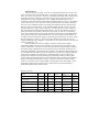
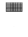
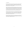
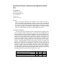
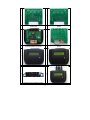
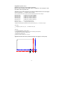
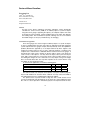
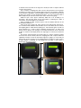
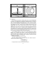
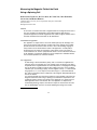
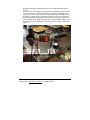
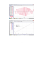
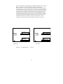
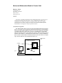
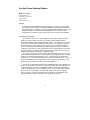
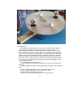
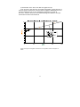
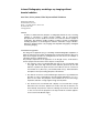
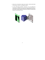
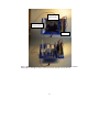
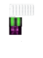
Table of Contents
1. *Microfluidics as Resistors in Simple Circuits
William Ashby, Christopher Easley
Auburn University
2. *Eddy Current Ramp
Brett Carroll
Green River Community College
3. *Independence of X and Y Motions
Brett Carroll
Green River Community College
4. *Cartesian Dive Team
Brett Carroll
Green River Community College
5. *Equipotentials Made Easy
Brett Carroll
Green River Community College
6. *Open Source Physics Laboratory Data Acquisition System v2.0
Zengqiang Liu
Saint Cloud State University
7. Center of Mass Visualizer
Zengqiang Liu
Saint Cloud State University
8. Measuring the Magnetic Field of the Earth using a spinning coil
Daniel Lund
California State University, Chico
9. *Concrete Operational Unit Converter
Robert A. Morse
10. *Mechanical Mathematical Model of Circular Orbit
Robert A. Morse
11. Fan Unit Driven Rotating Platform
Robert A. Morse
12. *Infrared Radiography: Modeling X-ray Imaging without Harmful Radiation
Otto Zietz, Kelsey Adams, Elliot Mylott, Ralf Widenhorn
* These apparatus can be built for less than $100.
Microfluidics as Resistors in Simple Circuits
William J. Ashby, Christopher J. Easley
Auburn University
179 Chemistry Building
Auburn, AL 36849
334-844-6966
[email protected], [email protected]
Abstract
This kit teaches Ohm’s law and the addition of resistors in series and parallel using
the visible flow of fluid through microfluidic channels that act as resistors (R). By
direct measurement of the flow rate (I) and fluid pressure (P=rho*g*h), the
resistance (R) for various configurations of parallel and series circuits can be
modeled and determined empirically. It was designed for hands-on learning by
discovery but is also suitable for classroom demonstrations.
Construction of Apparatus:
Materials Needed:
Aluminum foil
Food color (optional)
Post Magnetically Attachable Templates (post MATs, inquire with the author)
Magnets, NdFeB 1/16”diam x 1/8” long,
Alternatively, replace the two above items with a 2.75 or 3.0mm Harris Unicore
biopsy punch
Microfluidics’ mold (donated from microfluidic group)
Polydimethylsiloxane kit (Sylgard 184, Dow Corning)
Syringes, plastic
Tube-fitting tees, plastic barbed for 1/16” ID tubing
Tubing, tygon, 1/16” ID, 1/8” OD
Tools Needed:
Aluminum foil
Clamps
Double-sided tape
Drill bits, 1.7mm and 2.7mm diameter
Drill press
Razor blade or knife
Saw (hand or band saw)
Stop watch or timer
Scale
Vacuum pump and chamber
1
Use of Apparatus:
Construction
Generally, holes are punched into PDMS microfluidics in order to attach tubing and
connect syringes or pumps. This is an option you can consider. However, care must be
taken in order to avoid sealing the tubing against the bottom of the hole when inserting it into
the microfluidic device. Students are likely to make this error. In order to avoid this error
which would distract students from the learning goals of the hands-on activity, a set of post
magnetically attachable templates (post MATs) can be purchased from the inventor at cost.
Post MATs are held onto microfluidic molds with magnets underneath the mold and create
the tubing connections generally made by punching.
Fabrication of the microfluidic channels is as follows.
1.
Cut a sheet of aluminum foil about 1 inch larger on every side than the
microfluidic mold.
2.
Place the mold on the aluminum foil and fold the sides of the aluminum up to
make a reservoir 1/4” to 1/2” deep.
3.
Using double-sided tape, attach magnets underneath the tubing connection areas
of the mold. (Skip this step if punching holes instead of using post MATs). Then
attach post MATs to the top side of the mold.
4.
Mix PDMS in a plastic cup (10 parts base to 1 part curing agent by weight) and
stir well for at least 3 minutes.
5.
Remove the air bubbles by placing in a vacuum chamber for 20-30 minutes (or
alternatively by covering the cup tightly with plastic wrap and leaving overnight
in a freezer; allow it to warm to room temperature before reopening).
6.
Pour the PDMS prepolymer over the mold
7.
Bake at 50-60 Celsius for at least 3 hours.
8.
Prepare a partially cured approximately 5mm thick sheet of PDMS by preparing
PDMS as described in steps 3-4 and baking briefly (10-30 minutes) until PDMS is
no longer sticky and stringy but is still tacky to the touch.
9.
Remove aluminum foil from cured PDMS and microfluidic mold.
10.
With razor blade or knife carefully seperate the cured PDMS from the mold.
11.
Remove post MATs from cured PDMS (alternatively punch holes into PDMS).
12.
Place the cured PDMS as a hole or as individual units onto the partially cured
PDMS.
13.
Bake at 50-60 Celsius for at least 3 hours.
14.
Separate into individual units.
2
Educational Use
Pressure (analogous to voltage, V) sources are created by placing an open syringe in one
of the connecting holes of a microfluidic device. Trim off the tip of the syringe if too short and
narrow to fit in the connecting hole. The pressure through the microfluidic chip is determined by
the height of the water according to the formula P=rho*g*h (where g is gravity and h is the
height between the input and output of the water). Multiple microfluidic resistors can be
connected in series and/or parallel with the tubing and tubing fitting tee connectors. Place tubing
into the output of your circuit. This will be used to measure the flow rate. Ideally it should be
bent over to run horizontally and thus avoid changing the height between the input and output
during the course of the experiment. To prime the microfluidic channels, connect a syringe to
this tubing and use it to apply vacuum to the output. Visually inspect the circuit to make sure
that each component is flowing and not blocked with air. Once the microfluidic is primed, an
initial measurement of the amount of fluid in the output tubing can easily be recorded using a
ruler. After a certain amount of time (at least 30 minutes for my design), a second measurement
of the amount of fluid in the output should be taken. These measurements and the diameter of
the tubing is used to determine the change in volume during the specified time in order to get the
flow rate (analogous to current, I). Because of the large diameter of the input reservoir, any
change in fluid height will be negligible. Using Ohm’s law the collective resistance of the circuit
is easily calculated, R = V/I.
The Microfluidics as Resistors in Simple Circuits kit provides visible, tangible
understanding that directly and precisely translates to the first principles of electronics: flow,
voltage, and resistance. The kit also provides the kind of hands-on, student-designed modeling
and experimenting recommended in the Next Generation Science Standards. Based upon our
field testing with middle school and high school students at ABC Montessori (McDonough, GA),
we recommend that each student be given the opportunity to prime at least a single microfluidic
resistor before engaging teams in the process of designing simple series or parallel circuits,
predicting their resistance, and then measuring and calculating the resistance. Having paper
towels on-hand and using plain water is also recommended. Besides providing a well-received
platform for teaching basic principles of electric circuits, the kit can also be used as students
advance to create and test more complex models containing mixed series and parallel circuitry.
Furthermore, multiple inputs and outputs can be used in order to develop some hands-on
understanding of Kirchoff’s rules for circuits.
Materials and Costs
Material
Purchase
price
quant
ity
quantity
used
polydimethylsiloxane
$ 60.00
500g
100g
Magnets, NdFeB,
$
1.40
10
20
Tygon tubing 1/16" ID, 1/8" OD
$ 10.00
50ft
2ft
Syringe
$ 18.22
10
2
tee for 1/16"ID tubing
$
6.32
10
5
magnetite
$ 18.00
1kg
50 g
3
Cost per kit
$
12.00
$
2.80
$
0.40
$
3.64
$
3.16
$
0.90
Supplier
EllsworthAdhesiv
es.com
Catalog#
Sylgard 184
kit
KJMagnetics.com
BC22
5114K11
McMaster.com
McMaster.com
McMaster.com
PyroxLLC.com
7510A663
2808K178
post MATs
punch (alternative to post MATs
and magnets)
$
4.00
15
15
$ 12.00
1
1
Totals
$ 129.94
$
4.00
$
12.00
$
38.90
Donated
Microfluidic mold
Readily available materials
plastic ruler
aluminum foil
clamps
food color
scale
plastic cups
4
the author
TedPella.com
Eddy Current Ramp
Brett Carroll
Green River Community College
12401 SE 320th St.
Auburn, WA 98092
253-833-9111
[email protected]
Abstract
The Eddy Current Ramp shows how the forces on a moving magnet vary with the
amount of conductive material nearby. A magnet is rolled along a U-shaped
copper ramp having a variable depth. As the magnet rolls from the shallower end
into the deeper end of the ramp, eddy current forces increase as the amount of
copper near the magnet increases. The magnet slows until it is barely moving;
reversing the motion reverses the effect.
Construction of Apparatus:
The Eddy Current Ramp is constructed of three pieces of copper bar, each 1.5
feet long and 0.25 inches thick. The side wall pieces are 1.5 inches high, and the
bottom piece is 0.5 inches wide. The bottom piece is held between the two side
pieces with four brass thumb screws (iron and steel must be avoided in the design).
Holes and/or slots are machined in the ends of the side pieces to accommodate the
thumb screws, which are loosened to adjust the slope of the bottom if desired, and
tightened to hold the pieces in place. The rolling magnet is a pair of 1 inch by ¼
inch commercial neodymium magnets stuck together to form one disk. A brass disk
of identical size is added to allow the comparison between its motion and that of the
magnet.
Use of Apparatus:
Students are fascinated by eddy currents. There is something almost magical
about a force between a magnet and a non-magnetic material such as copper, and
the sheer enjoyment of seeing it in action is something they will always remember.
It’s a great way to draw their interest into all areas of magnetic induction such as
transformers, generators etc.
The Eddy Current Ramp allows students to see the effect of changing the
amount of conductive material nearby; how it changes the forces due to eddy
currents and thus the speed of the rolling magnet. And since the ramp is wide open,
the motion of the magnet is highly visible, unlike the closed tubes which are
generally used for this purpose.
The ramp can be set so that the depth varies continuously, or by loosening the
brass screws and moving one end of the ramp, it can be changed to a trough of
uniform depth. The varying depth arrangement allows students to see how
5
increasing the amount of conductive material affects the eddy current forces, while
the uniform depth trough arrangement can be used as a more visible replacement
for the usual hollow tube demonstration.
With the ramp set up with a varying depth, the shallow end of the ramp is placed
up on a wooden block to increase the slope of the ramp. The magnet is placed in
the shallow end of the ramp and released. At first it rolls quickly because there is
little copper next to the magnet, but as it rolls deeper into the ramp it slows down,
until in the deep end it is barely moving. Reversing the motion by putting the steep
end higher reverses the sequence, with the magnet rolling slowly at first, then
picking up speed as the walls fall away on the sides.
Repeating the motion with the brass disk shows that the changing speed is not
due to any frictional force, but strictly due to the eddy current forces on the magnet.
Changing the arrangement to a constant-depth trough produces a very slow motion
throughout, even when the trough is at a steep angle. The magnet can also be held
flat against the outside of one of the walls and released to slide down the side; even
this will produce a very slow motion with very high visibility.
6
Independence of X and Y Motions
Brett Carroll
Green River Community College
12401 SE 302th St.
Auburn, WA 98092
253-833-9111
[email protected]
Abstract
The independence of motion along two perpendicular axes X and Y when there is
acceleration along the Y-axis but not along the X-axis is a central part of
kinematics. This is often shown using a “shooter-dropper” in which one ball falls
vertically while the other is shot horizontally, both reaching the floor at the same
time. But that happens quickly and is difficult to follow by eye. This demonstration
slows the motion down and allows for variable motion along the X-axis, clearly
showing the independence of the two motions.
Construction of Apparatus:
This demonstration is built from two pieces cut from a 2 foot by 4 foot flat board.
Drawer slides are attached to the backs of the boards so that the smaller board may
be moved away from the larger board while staying parallel to it at all times.
Aluminum tracks are mounted on the upper surface of the boards so that steel balls
can be rolled down the tracks parallel to one another.
The entire apparatus is raised at one end by a wood block so that the aluminum
tracks are pointing down the slope at a small angle. A release mechanism at the
high end of the tracks holds the balls in place until it is lifted, at which point the balls
begin rolling down the track.
Use of Apparatus:
Understanding (and accepting!) the independence of X and Y motions is a crucial
part of learning physics. Many students find it hard to believe that a ball shot
horizontally while another is dropped vertically from the same height will both land at
the same time. Many feel that the horizontal motion ought to increase the time
required to fall, because the ball travels a greater distance. Convincing them that
the vertical acceleration of both balls (and thus time of fall) is the same regardless of
horizontal motion is often a challenge.
Standard demonstrations to illustrate this principle include the “shooter-dropper,”
where one ball is dropped vertically while another is fired horizontally from the same
height. Since their vertical accelerations are the same, both balls strike the ground
at the same time. While this is a good demonstration of the principle, it is in a sense
a special case of the effect, and also happens too quickly for the eye to follow both
7
balls. Students must simply infer that the vertical accelerations are the same from
the simultaneous landings of the balls.
This new demonstration is a method of overcoming those problems. Balls are
rolled down two parallel tracks, one of which can be moved on drawer slides at right
angles to the rolling motions. The acceleration down the track is analogous to
vertical acceleration in the shooter-dropper, being caused by the component of “g” in
the direction of the track. The horizontal motion of the track mounted on the drawer
slides is analogous to the horizontal motion of the fired ball.
When the balls are released simultaneously down the tracks and one track is
moved horizontally, the balls are seen to roll together in the “vertical” direction,
despite the horizontal motion of one track. This arrangement has two advantages.
The horizontal motion can be constant (as in the shooter-dropper), or it can be
moved in any fashion whatsoever without affecting the vertical motion of the ball. It
also slows the motion down so that the movements of the two balls can be easily
followed by the eye.
Students can easily see that the vertical acceleration stays the same despite any
horizontal motion of the track, a more general case than the shooter-dropper which
is limited to a constant horizontal velocity. And the lower acceleration of the balls
allows the students to see that the balls are always at the same position in the
vertical direction, giving them a clearer understanding of the concept of independent
motions in two perpendicular directions.
To operate the device, place the two balls above the release mechanism on their
respective tracks. Lift the release mechanism to start the balls rolling, then move the
smaller board in a horizontal direction. You can move it outward at a (reasonably)
constant velocity and the two balls will track vertically, analogous to the motions in
the shooter dropper but with much lower vertical acceleration. But a more
convincing case is to move the smaller board outward horizontally, then back in to its
original position. It’s easy to see that the vertical motions of the balls have stayed
the same despite the horizontal motion of one ball. And the fact that the horizontal
motion is completely arbitrary (the track can be moved in and out more than once if
desired) gives them a more general case of the principle than is possible with the
shooter-dropper. The improved visibility and increased flexibility of the horizontal
motion make for a more convincing case for the independence of two perpendicular
motions.
8
Cartesian Dive Team
Brett Carroll
Green River Community College
12401 SE 320th St.
Auburn, WA 98092
253-833-9111
[email protected]
Abstract
The Cartesian Diver is a venerable Physics demonstration, having been used for
over three centuries to teach about buoyancy and the relative compressibility of air
and water. But previous versions have used single divers, with no means of
making quantitative comparisons of what makes the diver sink. This new version
has three divers, close in volume but greatly different in mass, which show the
effect of mass (and thus density) of the diver on its performance.
Construction of Apparatus:
The Cartesian Dive Team is constructed of three pieces of transparent PVC tube,
glued into PVC “T” joints of corresponding size. Three divers (compressible
accordion bottles) are inserted into the three tubes and the tubes and joints are
glued together to form a sealed system. A compression piston tube is attached to
the tubes through a vinyl hose. A small pluggable hole is drilled in the top, through
which water is poured until the system in full and void of air except in the accordion
bottles.
The three divers have different amounts of weight attached to the bottom, so that
the volumes are nearly equal but the masses of diver + weight varies in an
approximate relation of 1:2:3. The masses are selected so that all of the divers float
at normal atmospheric pressure, but will sink upon compression. The compression
piston tube is used to increase pressure in the system and decrease the volumes of
the divers due to compression of the air inside
Use of Apparatus:
Cartesian divers are fun to watch as they glide elegantly up and down inside a
sealed tube, controlled only by the pressure exerted on the water in the tube. But
there has been no way to show how varying the properties of the divers changes
their behavior. No quantitative comparisons can be made with a single diver, so it is
impossible to show how divers of different properties (in this case mass) react to
equal pressure increases.
The Cartesian Dive Team has three divers in three interconnected tubes, each
diver having a different mass due to the extra masses fastened to the bottom. Since
the volumes of the divers are nearly equal, all will compress to equal volumes as
pressure in the system is increased by pushing upon the piston. Each will have an
9
identical buoyant force at all times (being simply equal to the weight of the water
displaced by each diver), but the heaviest diver will sink first because it is the first
one whose weight overcomes the buoyant force. As the pressure is increased and
the divers shrink further, the next heaviest diver will sink, flowed eventually by the
lightest diver. Slowly decreasing the pressure causes the divers to rise in the
reverse sequence.
The relative sinking times can be used for a discussion of density and buoyancy.
Each diver becomes denser on compression, and sinks when the density of the
diver is greater than that of water. Since the heaviest diver started with the most
mass, its density is the highest of the three, and it is the first whose density rises
above that of water and is thus the first to sink.
The Cartesian Dive team can also show that pressure in a liquid is transmitted
equally throughout a chamber. Each of the divers starts with about the same
volume, and as the compression piston is pushed in, each diver shrinks an equal
amount because the pressure on all three is equal despite their different locations
inside the system.
10
Equipotentials Made Easy
Brett Carroll
Green River Community College
12401 SE 320th St.
Auburn, WA 98092
253-833-9111
[email protected]
Abstract
Mapping electrical equipotential lines between conductors can be tedious and time-consuming.
The usual method is to find spots of equal potential on a gridded piece of conductive paper, note
the X-Y position of the spot on the grid, and transfer that spot to another piece of gridded paper.
This is repeated over and over until a sufficient number of equipotential spots have been mapped
to be able to draw an equipotential line joining them. The process is then repeated at a new
voltage. This new variation eliminates the need to transfer between grids, speeding up the
process and eliminating possible errors.
Construction of Apparatus:
The apparatus is constructed of two sheets of transparent acrylic, each slightly large than a
standard sheet of paper. They are bolted together with a ¾ inch spacer in between so that one is
directly above the other. A sheet of conductive paper is prepared by adding conductive copper
tape in any of a variety of shapes but including at least two conductive lines at some distance
apart. The conductive paper is then taped down on top of the lower sheet of acrylic, and a set of
batteries is attached to the copper tapes so that there is a difference in voltage between them.
Voltage probes are constructed of thin arms of acrylic, each having a round-headed nut and a
bolt at one end, attached to a wire that runs the length of the arm, plus an extra foot or so of wire
with a banana plug attached to the end. That is plugged into the voltage input jack on a
multimeter. The common jack on the multi-meter in connected by another wire to whichever of
the two copper conductors the user wants to call ground. The probe lead is slipped between the
two acrylic sheets and touched to the conductive sheet, where it provides a readout on the
multimeter of the voltage at that point, with respect to the common (ground) input.
Transparent versions of the conductive paper/copper tape shapes have been prepared on a
photocopier so that each is an identical match to the conductor layout. These are taped to the top
sheet of acrylic, above the conductive paper so that they line up with the layout of the conductors
below.
11
Use of Apparatus:
When voltage is applied to the copper conductors, an electric field is created on the conductive
paper. This field has lines of equal voltage, or equipotentials, at varying distances from the
copper conductors. These equipotentials can be mapped by touching the end of the voltage
probe down to the paper, and moving it around until the voltage equals the desired value for the
first equipotential line (say +1 volt above ground).
That point is then marked on the transparency by simply touching a sharpie to it at the position of
the probe’s sensing point (the nut at the end) and marking that spot. Then the probe is moved
until another spot of the same potential is reached, and that point is then marked with the same
color of sharpie by putting a dot above the sensing point of the probe. The process is repeated
until a sufficient number of points for that potential have been mapped, then an equipotential line
is created by joining the dots using the same-color sharpie. It often helps to place a white sheet
of paper underneath to provide better visual contrast for the dots while drawing the line.
Another value of potential is then chosen (say +2 V above ground) and the process is repeated
with a different color sharpie to find and mark spots with that potential and join them together
into a second equipotential line. The process is repeated again with a third equipotential, and so
on until the potential of the second conductor is reached. At that point a complete series of
equipotential lines has been mapped, and the transparency can be removed for display to the
class, or inserted into a lab report by the students.
This method of marking a transparency above the conductive paper eliminates the transferring of
dots between the conductive grid and a separate piece of gridded paper. That cuts the time
required to produce the equipotential lines dramatically, allowing for either a faster lab or demo,
or a greater density of equipotential points, or both
12
Open Source Physics Laboratory Data Acquisition System
V2.0
Zengqiang Liu
720 4th. Ave. S. WSB311
Saint Cloud State University
St. Cloud MN 56301
320-308-3154
[email protected]
Abstract
Open source physics laboratory data acquisition system V2.0 will connect to
sensors to perform physics laboratories. It works as a generic lab sensor interface
and accepts your C++ program to perform custom tasks. It costs less than $65 and
one hour to assemble. The new design greatly improved functionality, usability
while drastically reducing the difficulty to assemble. Wireless communication and
new low cost high quality sensors have also been added to the system.
Construction of Apparatus:
The open source physic laboratory has been redesigned from the original system
(V1.0). A number of low-cost open source sensors have been developed for this
system. A Bluetooth wireless transmitter is outfitted to the system to provide wireless
data transmission to any Bluetooth Serial enabled PC, tablet and smart phones. The
enclosure no longer requires extensive machining as before. It only requires one
small hole for the rotary encoder shaft, which can be made with a hand drill. A rotary
encoder with clickable shaft has replaced the 3-button layout to provide a more
intuitive user interface for up/down/enter. This also reduced the holes for buttons
from 3 to 1. The LCD window is pre-cut on the enclosure so there is no need to cut a
window on a face plate anymore. Also board mount DIN-5 connectors have replaced
panel mount connectors thus eliminated 12 wires and 24 wire leads for the
connectors. A battery clip is also included and a battery can be installed inside the
enclosure, instead of connected outside the enclosure. A power switch is added to
switch between the internal battery and external AC adapter, making it more flexible.
The above improvements have greatly reduced the time to construct the system and
drastically improved the functionality and usability of the system.
Item
Qty Unit price Subtotal
Open source physics laboratory DAQ V2.0
1
$50.00
$50
FTDI Basic Breakout USB-TTL (ebay)
1
$7.00
$7
Bluetooth serial adapter (ebay)
1
$7.00
$7
Table 1. Parts list of the apparatus.
13
A)
B)
Front side of the unpopulated
circuit board
C)
Back side of the unpopulated circuit
board
D)
Front side of the populated circuit
board mounted in enclosure
E)
Back side of the populated circuit
board
F)
Enclosed system
G)
Enclosed system power up screen
H)
Connector panel (3 DIN-5, Power
System measuring three sensors
14
barrel, 4-pin connector, switch)
I)
simultaneously
J)
Schematic diagram
Circuit board layout
Figure 1. Assembling the OSPL V2.0 and its features.
1) Obtain all parts listed in table 1.
2) Assemble the OSPL DAQ V2.0 according to instructions. Any 9V battery or
center-positive 2.1mm AC adapter with 7-12V 300mA DC output will be sufficient
to power the DAQ. The front and back sides of the circuit board are in fig.1-A-B.
An assembled kit is depicted in fig.1-C-D.
3) The 5-pin DIN sockets were used in the unit since older Vernier sensors use 5pin DIN plugs. Newer Vernier gauges use BTD connectors but you can purchase
an adapter to connect to DIN-5 connectors. You may also add ¼" stereo jacks for
photogates.
4) You can add a 4-pin connector to the port next the the DIN-5 connectors and use
a Vernier BTD cable to connect to Vernier and PASCO sonic rangers. Select
digital sensors in the menu.
5) Load a sample program to the DAQ box with the USB adapter via Arduino IDE
(code in appendix II).
6) Make your measurement either with the on-board display or with a PC.
Use of Apparatus:
This apparatus is capable of sensing most 5V analog sensors used in
introductory physics and science labs. A number of DIN-5(older) and BTA(newer)
Vernier sensors including force gauge, direct temperature, temperature, pressure
gauge, conductivity probe, etc. have been tested to work with this apparatus.
Besides analog sensors, it can also sense digital sensors such as sonic rangers,
photogates, rotation sensors and drop counters etc. when an appropriate adapter is
constructed to allow their connection. Moreover low-cost modern sensors with serial
and I2C interfaces that are not compatible with Vernier or PASCO data acquisition
systems can be connected to this system. Some of these sensor boards are as low
15
as a few USD while their commercial counterparts are hundreds of USD. This
includes high-g or precision 3-axis accelerometers, 3-axis gyroscopes, 3-axis digital
compass, cameras, sonic rangers, barometric sensors etc. A 10DOF sensor with 3axis accelerometers, 3-axis gyroscopes, 3-axis digital compass and a barometric
sensor only costs $13 online but would cost several hundred USD and may not be
used all simultaneously. In fact, one may find it hard to get a digital gyroscope
compatible with systems sold by popular teaching apparatus brands. Having a
decent set of sensors in a teaching lab and even at home becomes a reality with this
device. The device has a standard menu preloaded to work with a number of
sensors out of the box and can be easily reprogramed to work newer and untested
sensors with minimal programming effort. It can display data on its LCD, with
pause/resume, as well as transferring them to a computer via Bluetooth wireless
adapter or regular USB. The cost of this device is less than $65 and can be reduced
to around $30 per unit if one procures parts themselves and construct a dozen of
these units instead of one unit.
The following are five lines of code demonstrating the five steps to use a 5V
analog sensor:
Line 1: acquire data:
reading=analogRead(channel);
Line 2: scale data according to user's manual:
result=a*reading+b;
Line 3: clear on-board LCD:
lcd.clear();
Line 4: display result:
lcd.print(result);
Line 5: pause momentarily for user to read the result:
delay(200);
If one replaces line 4 with Serial.print(result), then the result will show up on a PC
when the unit is connected to the PC Bluetooth serial port. Appendix I lists the
specifications of the DAQ while Appendix II is a sample program.
Appendix I: specifications.
Microcontroller: ATMEGA328P-PU with Arduino Uno optiboot bootloader
Program memory: 32KB, roughly stores up to 3,000 lines of C/C++ code.
Variable memory: 2KB, roughly stores up to 1,000 data points.
EEPROM: 1KB, roughly stores up to 500 data points.
Bluetooth serial port supports 115,200 baud rate wireless data transfer.
Available pins: 6 analog pins and 2 digital pins. Analog pins can also be used as
digital pins.
Supports up to 3 DIN-5 style analog sensors with autoID (resistor-based) or up to 6
analog sensors without autoID (need to make custom cables)
Supports up to 8 digital inputs or outputs for photo gates or 4 sonic rangers.
Supports serial and I2C sensors, which may need some programming.
On-board 16X2 character LCD monitor with back light
On-board speaker
LCD back light jumper to disable back light to preserve battery power
Programmer port for program upload and data link with a PC/Linux/Mac
Rotary encoder for more intuitive menu navigation and faster number entry
16
Regulated 5V power source
Ready-to-use enclosure (only need one small hole)
Massive amount of library and sample codes as templates to start a project or load
pre-written code for specific tasks.
Appendix II: One sample program to be loaded via Arduino IDE version 1.0 or higher
#include <LiquidCrystal.h>
///< Include the liquid crystal library
//These describe how the LCD is connected to the development kit and need not be changed.
#define LCD_RS 2
///< Arduino pin connected to LCD RS pin
#define LCD_EN 3
///< Arduino pin connected to LCD EN pin
#define LCD_D4 4
///< Arduino pin connected to LCD D4 pin
#define LCD_D5 5
///< Arduino pin connected to LCD D5 pin
#define LCD_D6 6
///< Arduino pin connected to LCD D6 pin
#define LCD_D7 7
///< Arduino pin connected to LCD D7 pin
#define lcd_rows 2
#define lcd_columns 16
///< Specify the height of the LCD.
///< Specify the width of the LCD.
LiquidCrystal lcd(LCD_RS,LCD_EN,LCD_D4,LCD_D5,LCD_D6,LCD_D7); ///< Create the lcd object
void setup()
{
lcd.begin(lcd_columns, lcd_rows);
}
///< Initialize the lcd object.
void loop()
{
int reading=analogRead(2); // Read channel 2
float result=(reading*5.0/1024)*(-4.9)+12.25; // Convert reading to physical quantity
lcd.setCursor(0,0); // Set where to display result
lcd.print(result); // Display result
delay(200); // Delay for human eyes to respond.
}
Appendix III: Drill hole location (rounded rectangle also appears on front panel)
0.08
17
Center of Mass Visualizer
Zengqiang Liu
720 4th Ave. S. WSB 324
Saint Cloud State University
Saint Cloud, MN 56301
320-308-3154
[email protected]
Abstract
An open source physics laboratory V2.0 data acquisition system dynamically
calculates the center of mass (COM) of an arbitrary object or system of objects
using three force gauges supporting the object(s). A computer captures live video
of the object(s) with a webcam, overlays COM location on the video, then displays
the resulting video. This visualization is dynamic, allowing users to see in real time
how COM changes as mass(es) and distance(s) are changing.
Construction of Apparatus:
Three force gauges are used to weigh an arbitrary object or a system of objects
on top of a weighing plate. An open source physics laboratory V2.0 data acquisition
system acquires the force gauges' outputs, then dynamically solves the equilibrium
problem (illustrated in appendix I) of an object balanced by three supports and
outputs the solution (center of mass x, and y, and total weight) to a computer. The
computer has a webcam that is calibrated with the locations of two force gauges. It
then marks the center of mass location on the live video to show a user where the
center of mass of the object is. You may move the object, take a part of the object
away, add or remove objects to see how the center of mass location changes as you
are making the changes. A user is welcome to use any object as long as its weight
does not exceed about 25N. You may take snapshots of the screen with the snap
shot button to save the image for later.
To construct the apparatus, you need the following parts:
Item
Qty Unit price Subtotal
Vernier force gauge
3
$109.00
$327
Open source physics laboratory DAQ V 2.0 kit
1
$64.00
$64
Sony PS3 Eye webcam
1
$30.00
$30
One will also need a PC computer and a tripod to set up the visualizer program.
Any PC with windows XP or better will be sufficient. You may connect the DAQ to
PC via Bluetooth if the PC is equipped with a Bluetooth adapter.
The optional laser cut pieces include a large disc with a small circular cut out
(can be inserted back) half the diameter of the large disc and inscribing the large
disc. This is a classic question in introductory physics. The expected center of mass
18
is marked on the back side of the large disc should you want to compare with the
system's measurement.
First, construct a weighing plate with L=15cm, with placement of force gauges
according to the figure 1E. The weighing plate needs not to be perfectly symmetric
as tare function is provided to remove the plate from the measurement. Next, attach
all three force gauges to their designated locations. You may need three BTA to
DIN-5 adapters if you have the newer version of the Vernier force gauge.
Build the open source physics laboratory DAQ from a kit according to its
instructions. This may take about an hour and requires a soldering iron, solder, a
screw driver, and a hand drill for one small hole.
After you build the DAQ, load the project code via Arduino IDE that can be
downloaded at arduino.cc.
Hook up the force gauges left, right, and top to the DAQ analog channels 0,1,
and 2. Start the DAQ. Click the knob to dismiss start screen. When you are sure that
the weighing plate is stable without anything on it, click the knob again. You will see
the live display of x, y center of mass coordinates and total mass. To pause, turn
knob to left. To unpause, turn left again. To start data transmission to PC, turn knob
to right. To return to local display mode, turn right again. To restart, press down the
knob.
On your PC, install the driver of the Sony PS3 eye. start the visualizer program
and mount the camera directly above the weighing plate with a tripod. Follow the
calibration instruction to click the left and the right force gauges on screen and you
will be ready to place an object on the weighing plate to visualize its center of mass.
A green marker is displayed for each gauge (left and right). A red marker is
displayed for the center of mass.
A)
B)
System power up screen
C)
Displaying center of mass and mass
D)
19
Live video (green crosses are left
and right force gauges, red cross is
COM)
E)
Transmitting Data to PC
F)
Force gauge placement top view
Demonstration piece (circular cutout
(L=15cm)
has half the radius of the disc)
Figure 1. Center of Mass Visualizer
Use of Apparatus:
This apparatus can be used to visualize center of mass of any extended object
as well as a system of point masses. The maximal weight of the object is 30N minus
the weight of the weighing plate (depending on what material you use to make it
with). I recommend getting the demonstration pieces, which is shown in the figure.
This one is a classic question in introductory physics. You can show the center of
mass calculation to your class and confirm your calculation with this visualizer and
suspending the piece with a string. You may also place several masses on the
weighing plate, one at a time, to observe how the center of mass is affected by
adding masses to the system. You may also move them with a pencil and show your
class how the center of mass is affected by the rearrangement as you are
rearranging them. You can easily set up a calculation question for a system of point
masses, then solve the question by placing the masses at the locations given in your
question. You can also very easily demonstrate that the center of mass of two point
masses always lies along the line that connects the two objects.
In static equilibrium chapter, you may use this visualizer again but for a different
purpose. You can challenge your students to come up with the formula that the
visualizer uses to find the center of mass. You may also challenge some more
advanced students with the mathematics used to scale, rotate, and translate the
physical location of COM to the display locations. Seeing the calculations will make
them appreciate the importance of mathematics.
Appendix I: Calculations
FL, FR and FT are measured by the force gauges.
Take x-axis as AOR for torques in x direction. Take y-axis as AOR for torques in
y direction. We find solutions as below:
Ftotal=FL+FR+FT (1)
x_com=(FR-FL)L/Ftotal (2)
y_com=FTL/Ftotal (3)
To display COM, one needs the following transformations:
20
(x_math,y_math)=[S][R](x,y)+(x_offset,y_offset), where [S] is a scale operation to
take mm unit into pixel unit, [R] is a rotation operation to rotate COM location since
the two force gauges may not be forming a horizontal line in video during calibration,
and (x_offset,y_offset) is the center of the two force gauges. [S], [R], and
(x_offset,y_offset) are calculated after the calibration.
(x_screen,y_screen)=[Iy](x_math,y_math)+(0,image_height), where [Iy] is an
inversion of y coordinate only and (0,image_height) is usually (0,480). This
transformation converts mathematical locations with origin on bottom left and y-axis
pointing upwards into screen locations with origin on the top left corner and y-axis
pointing downwards.
Appendix II: program code for the OSPL V 2.0
The program is rather long. Please contact the author for an electronic copy.
Appendix III: program code for the PC video visualizer
The program is rather long. Please contact the author for an electronic copy.
21
Measuring the Magnetic Field of the Earth
Using a Spinning Coil
Daniel Lund, Jaydie Lee, Dr. Eric Dietz, Dr. Xueli Zou, Chris Kaneshiro,
Steven Sun, and Robert Blanton
California State University, Chico, Department of Physics, 95929-0202
(530)-481-5863
[email protected]
Abstract
A coil of wire is rotated in the earth’s magnetic field. The voltage observed across
the coil is related to the magnitude of the incident magnetic field. Using a
specialized apparatus, both the magnitude of the earth’s magnetic field as well as
the field’s inclination from horizontal can be determined.
Construction of Apparatus:
The apparatus is composed of a coil of wire held in place by two bearings such
that it can be rotated. Two bushings at either ends of the rotating coil assembly
provide electrical connections to the coil wires. One of the bushings engages a
rotary motion sensor mounted to the frame of the apparatus. A small pulley is
mounted on the far end of the shaft of the rotary motion sensor. The frame is
constructed from 1/4" and 1/2" polycarbonate sheet. Feet are attached to the base
of the apparatus such that the apparatus can be clamped to a worktable with the
axis of rotation parallel to or normal to the table.
Use of Apparatus:
A small string is wound around the pulley, and a constant force applied to the
string by means of a hanging mass. The rotation of the coil along an axis that is
not parallel to the magnetic field of the earth will produce a changing flux through
the coil, by which a voltage is induced. The voltage across the coil is recorded
770 times per second using a laptop, and the angular velocity, , is inferred from
the graph of Vpp vs. t. The slope of a linear fit for Vpp vs  can be determined.
The slope is proportional to the component of the magnetic field perpendicular to
the axis of rotation.
It is worth noting that there have been numerous other attempts to measure the
magnetic field of the earth using a spinning coil, and that this experiment is not
completely unique. However, the design of this apparatus is a change from an
older apparatus that is now obsolete. This new apparatus is simpler, more
aesthetically pleasing, compact, and doesn’t require an electric motor to rotate
the coil. David Kagan1 presents an article detailing measuring of the earth’s
1
Kagan, David T. 22
magnetic field using an older apparatus that was used in introductory physics
courses.
To measure the vertical component of the field, the apparatus is aligned so that
the axis of rotation is oriented north-south (via a compass) and parallel to the
surface of the earth. To measure the horizontal component of the field, the axis
of rotation is aligned so that it is normal to the surface of the earth. From these
measurements both the magnitude and inclination of the earth's magnetic field
can be determined. An image of the apparatus is displayed below in figure 1, and
the arrangement of a hanging mass used to drive the coil rotation is displayed in
figure 2.
Figure 1: apparatus configured for operation
"Measuring the Earth's Magnetic Field in an Introductory Laboratory with a
Spinning Coil" in The Physics Teacher, Oct. 1986, 423-424. 23
Figure 2: hanging mass configuration
The results from a run of data collection with the apparatus are shown below in figure 3, a graph
of coil voltage versus time. By inferring the frequency of rotation from the oscillations, a graph
of induced voltage amplitude versus angular frequency can be produced, and a linear fit can be
determined. This slope is directly proportional to the magnetic field incident upon the coil. This
graph is shown below in figure 4.
24
Figure 3: voltage induced in spinning coil
Figure 4: voltage amplitude vs. angular frequency
25
Concrete Operational Unit Converter
Robert A. Morse
5530 Nevada Ave
Washington, DC 20015
202-537-0759
[email protected]
Abstract
Many students have difficulty with unit conversions. This demonstration device is a
concrete embodiment of the mental process of replacing one unit by its equivalent
in another unit. My anecdotal experience with this device is that it helps a certain
group of students figure out how to convert units.
Construction of Apparatus:
A section of white board about 30 cm square is mounted on a base so it will
stand vertically. Two shelves, each about 7 cm by 15 cm are mounted on the right
hand side of the front surface. One is just above the base, the other about half-way
up. Several rectangular parallelepipeds with square cross section about 5 cm by 5
cm by 12 cm are constructed from manila folder material. One face of each is
labeled with a unit of measurement and the other faces with the equivalent number
of units in some other system. Examples:
{1 mile; 5280 feet; 1760 yard; 1.609 kilometer}
{1 foot; 12 inches; 30.48 cm; 0.3048 meter}
{1 hour; 60 minutes; 3600 seconds; 1/24 day}
{1 pound; 16 ounces; 4.448 newtons; 444 822 dynes}
Materials Cost:
All materials used were scavenged.
White board - part of a 1/8 inch by 4 ft x 8 ft white gloss finish hardboard panel.
Cost of one panel is about $13 and would make 32 pieces of the size needed. Cost
about $0.50
Shelves made of corrugated cardboard from cardboard box – free.
4 bolts to support shelves – cost $1.40
Total cost about $2
Use of Apparatus:
Many students have difficulty with unit conversions. This demonstration
device is a concrete embodiment of the mental process of replacing one
unit by its equivalent in another unit. My anecdotal experience with this
26
device is that it helps a certain group of students figure out how to convert
units. To illustrate a conversion, consider converting 75 miles/hour to
feet/second. Write 75 with a whiteboard marker on left area of whiteboard. Place
the parallelepiped or “unit box” with 1 mile on its face on the upper shelf and the
1 hour unit box on the bottom shelf. Rotate the 1 mile unit box about the long axis
to show the face with 5280 feet and rotate the 1 hour unit box to show the face
with 3600 seconds (See figure). Finish the conversion by multiplying 75 times
5280 and divide the result by 3600. If a simple conversion of miles to kilometers
is required, the bottom shelf would not be used. The intent of this device is not
that students should carry around a lot of unit boxes, but that the concrete
example of the process will facilitate internalizing a “model” of the process.
75
1 mile
75
1hour
5280 feet
3600 sec
Initial setup
conversion
Final step 75 x(5280/3600) ft/sec = 110 ft/sec
27
Mechanical Mathematical Model of Circular Orbit
Robert A. Morse
5530 Nevada Ave
Washington, DC 20015
202-537-0759
[email protected]
Abstract
This device, a mechanical instantiation of the mathematical model of a circular orbit, is
intended to help students think about how a variety of mathematical formulae can be
assembled to give a flexible description of a physical situation. Many of my students,
particularly those less fluent in algebra, have found such mechanical models help them
understand how to use algebra to analyze a particular situation.
Construction of Apparatus:
This demonstration device consists of a base board about 30 cm long cut from a
piece of 1 by 3 pine. For this particular mathematical model there are two quantities
that can be represented by different expressions, and each quantity has a periaktos,
a rotatable paper prism, with 7cm by 7 cm faces assembled from a manila folder
which pivot vertically about an axis made from a pencil or dowel inserted in a hole in
the base. One periaktos is a triangular prism and the other is a cube. An additional
piece cut from a manila folder is fastened to the front of the base and has an equals
sign, a division indicator and a third quantity written on it.
Circular Orbit Model
periaktoi
ac
pivot
Fg
Manila folder
piece
pivot
msat
base
28
The cubical periaktos for the centripetal acceleration has four faces labeled as
follows:
2π v
4π 2 Rorbit
v2
T
T2
R orbit
ac
The triangular periaktos for the gravitational force has three faces labeled as
follows:
Fgreav
gmsat
G
M cb msat
2
Rorbit
Materials:
Two manila folders – from office supplies – cost - a few pennies
One 30 cm or so piece of 1 by 3 pine – scavenged from scrap – cost under $1
Two pencils – cost about $0.25 each
Use of Apparatus:
This device, a mechanical instantiation of the mathematical model of a circular orbit, is
intended to help students think about how a variety of mathematical formulae can be
assembled to give a flexible description of a physical situation. The particular model here is
that of a satellite in a circular orbit, but other models could be readily constructed on the
same principles. In its initial configuration, the device displays Newton’s second law in the
form
Fgrav
msat The terms for the acceleration and the gravitational force are each written on
one face of a periaktos, a term from classical Greek stagecraft meaning a
many-sided prism that can be rotated to change the scene. Here rotating each face of the
acceleration prism has one of the expressions for centripetal acceleration in terms of
velocity and period, orbit radius and period or velocity and orbit radius. The gravitational
force prism has three faces, one giving the expressions for gravitational force in terms of
the masses of the satellite and central body, the orbital radius and the gravitational
constant, and the other giving the force in terms of the local gravitational field strength
and the mass of the satellite. The mass of the satellite in the denominator does not rotate,
since there is no alternate expression for it. In use, a student can rotate each of the
periaktoi to an expression that corresponds to the information that he or she has or is
trying to find for a particular orbit situation. The intent of this device is help students
understand how to think about physical quantities in terms of their relationships with
other quantities. It serves as a concrete example of what is an otherwise invisible process
in the head. It has been my observation, based on student reactions, that for a certain
ac =
29
group of students devices like this are a bit of a revelation and help them to figure out the
kind of processes that can be used to analyze situations.
30
Fan Unit Driven Rotating Platform
Robert A. Morse
5530 Nevada Ave
Washington, DC 20015
202-537-0759
[email protected]
Abstract
An inexpensive rotating platform driven by small fan units and an accompanying
set of masses allows students to design investigations relating torque, moment of
inertia and angular acceleration. Fan units may be placed in different locations and
at different angles, and the number and distribution of masses may be easily
changed. Data is collected using a rotary motion sensor, interface and computer.
Construction of Apparatus:
The apparatus consists of a circular platform with a radius of 30 cm cut with a
bandsaw or a good sabre saw from a ¼ inch thick sheet of medium density
fiberboard (available at Home Depot and other outlets – a ¼ inch by 2 ft x 4 ft panel
costs about $7 and makes two platforms). The panel has a center hole sized to fit
over the pulley on a rotary motion sensor (Vernier sensor used in this example).
Holes ¼ inch diameter are drilled along 8 radii starting 10 cm from the center and
continuing at 5 cm intervals. The rotary motion sensor is supported by a 55 cm piece
of pine 1x4 with a ½ inch dowel inserted near one end to clamp the sensor to. The
board is then clamped horizontally to a laboratory table.
The masses are made of concrete mortar mix cast in PVC end caps for 1.5 inch
PVC schedule 40 pipe and come out to be approximately 200 grams. They are quite
inexpensive compared with laboratory masses, costing about $1.50. Before the
concrete is cast, a ¼ inch hole is drilled in the center of the end cap and a 1 inch ¼ 20 bolt is threaded from the inside to stick out the end of the cap. The masses can
now be fastened in different locations on the rotating platform.
The forces are provided by small fan units adapted from those described by R. A.
Morse, Fan Unit Physics, The Physics Teacher vol. 43(3) p 162. See that article for
construction details. The units are modified by drilling a ¼ inch hole in the bottom
center of the battery box cover and putting a ¾ inch ¼ -20 round head bolt through
the hole. (The cover should be secured with duct tape as otherwise it may pop
loose.) Fan units can now be mounted at various positions on the platform, and
directed at various angles, held in place with wing nuts. See picture.
31
Use of Apparatus:
This apparatus was designed for use in a unit on rotational motion. Students
were reminded that Newton’s second law describes linear acceleration as
determined by the combination of forces exerted on an object or system and the
mass of the object or system. They are shown a set of the apparatus consisting of
up to six fan units, eight masses, the platform, sensor, interface and computer and
asked to come up with experimental designs to determine what factors affect the
angular acceleration. They are given the constraint that for the sensor to operate,
the system must be balanced. They can request other laboratory equipment if they
wish. Students are then broken up into groups to discuss possible designs, which
are presented to the class.
The equipment allows investigations of:
1) effect of different amount of force by having one, two, three or four fan units
operating
2) effect of different locations for force application by having fan units at different
radii
3) effect of different directions of force relative to the radius vector
4) effect of counteracting forces at same or different radii
5) effect of different total amounts of mass
6) effect of mass location and determination of rotational inertia
32
7) determination of the effect of the disk from graph intercept
In my classroom, after discussion of possible investigations, groups drew lots so
that each group carried out two of the possible investigations identified by the class
and then compared results for the overlapping investigations in a wind up
discussion. After the discussion, the formal terminology and definitions of torque
and moment of inertia were introduced.
Graph of reciprocal of angular acceleration versus product of mass and square of
radius
33
Graph of angular acceleration vs. angle of thrust fit with sin curve
34
Infrared Radiography: modeling x-ray imaging without
harmful radiation
Otto Zietz*, Kelsey Adams, Elliot Mylott and Ralf Widenhorn
Department of Physics
Portland State University
SRTC, 1719 SW 10th Ave., Room 134
Portland, OR 97201
*[email protected]
Abstract
A device to demonstrate the principles of radiography without the use of ionizing
radiation is presented. It utilizes infrared radiation and an up-converting
phosphorescent screen to probe the contents of an enclosure which is opaque to
visible light. The apparatus enables students to explore concepts in radiography
including properties of electromagnetic radiation, attenuation, image formation,
differences between planar x-ray imaging and computed tomography, and digital
and analog imaging.
Construction of Apparatus:
The design of our apparatus (Fig. I) is modeling standard radiographic equipment, in
which an emissive source and an analog detector are placed on opposite sides of an
object to be imaged. Instead of an analog detector one can also use, for example, a
cell phone camera as a digital sensor.
The principle components of the apparatus are an IR light source, an IR detector,
and an opaque enclosure where various objects can be placed:
 The emissive source, an infrared LED array (Fig. II), was constructed using
forty eight SFH 4547 high intensity LEDs (950 nm) powered by four 9V
batteries in parallel. The peak emission of the LED was chosen such that it
was invisible to us (like x-rays), not harmful (unlike x-rays), and matched the
absorption of the up-converting phosphor of the detector.

The detector screen was constructed through suspension of 1g of IRUCG- IR
phosphor in 8 mL of polyurethane and subsequent application to a 3” x 2”
piece of cross-stitch. The phosphor screen absorbs two or more low energy
IR photons and emits a single, higher energy 552 nm photon.

The enclosure was constructed from a display case covered with a Congo
Blue filter #181. The base platform was made such that the detector can
move laterally away from the enclosure, allowing the enclosure to be rotated
so one can see how the projection of an object inside the container appears
on the screen from different angles.
35

A lid was also constructed to hang over the detector, reducing ambient light
and allowing for viewing in normal lighting conditions.

A slide demonstrating differential attenuation (for x-ray imaging this
corresponds to radiodensity and is measured on the Hounsfield scale) was
constructed from two filters (Congo Blue #181 and Medium Blue Green #877)
and a piece of paper. Stands for the LED array, detector, and attenuation
slide were constructed from acrylic.
36
Enclosure with
Objects Inside
Up-converting
Phosphor Detector
IR LED
Figure I: Radiography apparatus comprised of an infrared LED array, objects concealed in a container
mostly opaque to visible light but mostly transparent to IR, and a phosphor screen for detection.
37
Figure II: Diagram of infrared LED array for use in radiography apparatus; voltage source is comprised of
four 9V batteries in parallel.
38
Figure III: Planar images of concealed objects from two angles with both analog (Phosphor Screen: left
panels) and digital (Cell phone Camera: right panels) detectors, displaying the differences in information
attained from each vantage point. The left panels represent in radiological terms an analog (phosphor screen
representing the x-ray sensitive plate) to digital conversion (digital image of the phosphor screen representing
the digitizing of x-ray images to a portable DICOM imaging file).
Component
Cost
Source
48x SFH 4547 IR LED
20.54
http://www.digikey.com/product-detail/en/SFH%204547/475-3002-ND/3461837
1g IRUCG- IR Phosphor
8.86
http://www.maxmax.com/aIRUpConversion.asp
Rosco #877 Filter
7.50
http://www.stagelightingstore.com/Stage-Lighting-Store/Dinshah-Gel-Cuts/RoscoRoscolene-877-Medium-Blue-Green-6-5-x-6-5-Cut
6x ½ W 1 OHM Resistors
0.84
http://www.digikey.com/product-detail/en/CF12JT1R00/CF12JT1R00CT-ND/1830445
IC Board
0.99
http://www.mcmelectronics.com/product/214590&scode=GS401&CAWELAID=220241326
4x 9V Battery
5.0
http://www.amazon.com/UltraLast-Alkaline-General-Purpose-Battery/dp/B002KT7URA
Display Case 44020
2.99
http://www.containerstore.com/shop/collections/display/cubesCases?productId=10000577
10”x 10” Congo Blue Filter
2.99
http://www.amazon.com/181-Congo-Blue-Filter-Sheet/dp/B004GE67SK
4x 9V Battery Connectors
2.36
http://www.digikey.com/product-detail/en/BS6I/BS6I-ND/32055
2x 12” x 12” Acrylic Sheet
8.70
http://store.gissn.com/Sheet-Acrylic-Clear-0-093-T-12-x-12-In-p/1unk3.htm
4x Terminal Blocks
2.00
http://www.digikey.com/product-detail/en/1776275-2/A98036-ND/1826899
2 Way Switch
0.29
http://www.digikey.com/product-detail/en/EVQ-11U09K/P8085SCT-ND/259570
Instant Adhesive
1.05
http://www.grainger.com/Grainger/SUPER-GLUE-Instant-Adhesive-3EHP6?Pid
Wire
negligible
Solder
negligible
Cross-stitch
negligible
Scrap Acrylic
negligible
8ml Polyurethane
negligible
Poster Tape
negligible
2x 2”Objects
negligible
Total Cost
64.11
39
Use of Apparatus:
To image the interior of objects opaque to visible light, radiography utilizes x-rays
and gamma rays. In the medical field, this technique has become a ubiquitous
diagnostic tool. The varying attenuation coefficients of air, water, tissue, bone or
metal implants within the body result in non-uniform transmission of radiation.
Through the detection of transmitted radiation, the spatial organization of materials
in the body can be ascertained. The thickness and large attenuation coefficients of
biological materials require the use of high energy x-ray radiation which can, for
example, cause DNA damage. Because of the potential harmful effect of x-rays,
demonstrations of this imaging technique are difficult to perform safely.
The goal of this apparatus is to use non-ionizing radiation to demonstrate
radiography. The device presented employs an array consisting of infrared light
emitting diodes as a radiation source and an up-converting phosphor screen as an
analog detector. The phosphor converts the invisible IR light and makes it visible to
the observer. While invisible x-ray radiation is used to look inside the human body,
we use invisible IR radiation to look inside an opaque enclosure. A cell phone
camera can be used as a digital detector as well. Qualitative comparisons can be
made between the analog phosphor detector and the digital smart phone detector
(the intensity of the IR radiation is such that it can be seen by most cell phones even
though they employ an IR filter, an exception is, for example, the iPhone 5 which has
a very strong IR filter). In both the x-ray and infrared cases, one cannot visually see
what is inside the object and the imaging method results in a two dimensional
projection of a three dimensional volume. By exploring how the presented apparatus
functions, students have the opportunity to investigate topics such as attenuation,
light absorption, image projection, the calculation of photon energies, or the
electromagnetic spectrum and its applications in medicine.
Two activities have been developed for this device. In the first activity, students
explore attenuation: the effects of material properties on the propagation of
electromagnetic radiation. This is accomplished with an array of optical filters,
varying in attenuation coefficients, placed between the emitter and detector.
Students are asked to observe the intensity of infrared light seen on the detectors
and compare them to each other as well as to analogous parts of the human body.
For example, the Congo Blue filter is largely transparent to IR light, similar to how
skin tissue is largely transparent to x-rays. The Medium Blue Green #877 is on the
other hand blocking a fraction of the light and resembles organs in radiological
images.
Attenuation and Transmission
Procedure:
 Place the Attenuation Slide between the emitter and the phosphor detector

Press the button to activate the LED array and observe the analog image.

Remove the phosphor screen and position your cell phone camera so that
the slide is between your camera and the LED array.

Press the button to activate the LED array and observe the digital image.
40

Describe the difference in transmission of radiation through each filter, the
relative attenuation coefficients of each component, and compare and
contrast detection methods (analog and digital). Here students can also
discuss that lenses are used in a cell phone camera while digital x-ray
sensors cannot employ lenses to focus the x-rays.
In the second activity, students explore planar imaging. An enclosure surrounded by
material that transmits infrared light but absorbs visible light causes the identity and
position of any objects inside to be obscured from sight. The students may discover
that a two dimensional image of a three dimensional object may not always suffice to
distinguishing the unknown objects. For example, if two objects are in the enclosure,
an image from only one angle may not provide the orientation, number, or shape of
the objects. Through illumination by the IR source and rotation of the enclosure,
students can view the contents of the box from multiple angles and thereby discern
the shape and orientation of objects contained within. This activity can serve as an
introduction to computed tomography.
Planar X-ray Imaging
Procedure:
 Place the container between the LED array and the phosphor screen. Insure
that the phosphor screen is positioned close to the container.

Press the button to activate the LED array and to observe the analog image.
Remove the phosphor screen and use a cell phone camera to observe the
digital image.

Draw the planar image from this viewpoint.

Replace the phosphor screen, rotate the container 90 degrees. Bring the
phosphor screen back into its initial position and view the analog image.

Remove the phosphor screen and use a cell phone camera to observe the
digital image.

Draw the planar image from this viewpoint.

Using the two images, describe the spatial arrangement of objects in the
container. Open the container and compare the positions with your
expectations.
Throughout this exercise, students can compare analog and digital imaging through the
use of the detector and their own cell phones, as well as comparing the components of
the apparatus to actual radiographic equipment. Further experiments using this device,
including examination of contrast agents, collimation techniques, and image clarity
enhancement can be designed with minimal changes to the core components.
This device allows for safe, interactive, and engaging exploration of topics covered in
undergraduate physics and biology courses for pre-health and life-science majors
without the high cost of specialized equipment and the danger associated with high
energy radiation. Students can experiment with electromagnetic radiation in real time by
probing the contents of an opaque enclosure and imaging unknown objects inside. This
hands-on demonstration renders the classically difficult and abstract concepts of
electromagnetic radiation and attenuation approachable and fun.
41
Apparatus Competition
2013 Summer Meeting of the
American Association of Physics Teachers
Sponsored by the
AAPT Committee on Apparatus
Prizes are generously provided by
American Association of Physics Teachers
One Physics Ellipse • College Park, MD 20740-3845 • www.aapt.org
Apparatus descriptions also available at:
groups.physics.umn.edu/demo/apparatus.html