1
on
si
er -0
V .2
0
Programming with Big Data in R
Speaking Serial R with a Parallel Accent
Package Examples and Demonstrations
pbdR Core Team
Speaking Serial R with a Parallel
Accent (Ver. 0.2-0)
pbdR Package Examples and Demonstrations
February 17, 2014
Drew Schmidt
National Institute for Computational Sciences
University of Tennessee
Wei-Chen Chen
Department of Ecology and Evolutionary Biology
University of Tennessee
George Ostrouchov
Computer Science and Mathematics Division,
Oak Ridge National Laboratory
Pragneshkumar Patel
National Institute for Computational Sciences
University of Tennessee
Version 0.2-0
c 2012–2014 pbdR Core Team. All rights reserved.
Permission is granted to make and distribute verbatim copies of this vignette and its source
provided the copyright notice and this permission notice are preserved on all copies.
This manual may be incorrect or out-of-date. The authors assume no responsibility for errors
or omissions, or for damages resulting from the use of the information contained herein.
This publication was typeset using LATEX. Illustrations were created using the ggplot2 package
(Wickham, 2009), native R functions, and Microsoft Powerpoint.
Contents
List of Figures . .
List of Tables . . .
Acknowledgements
Disclaimer . . . . .
I
.
.
.
.
.
.
.
.
.
.
.
.
.
.
.
.
.
.
.
.
.
.
.
.
.
.
.
.
.
.
.
.
.
.
.
.
.
.
.
.
.
.
.
.
.
.
.
.
.
.
.
.
.
.
.
.
.
.
.
.
.
.
.
.
.
.
.
.
.
.
.
.
.
.
.
.
.
.
.
.
.
.
.
.
.
.
.
.
.
.
.
.
.
.
.
.
.
.
.
.
.
.
.
.
.
.
.
.
.
.
.
.
.
.
.
.
.
.
.
.
.
.
.
.
.
.
.
.
.
.
.
.
.
.
.
.
.
.
.
.
.
.
.
.
.
.
.
.
.
.
.
.
Preliminaries
v
vi
vii
1
2
1 Introduction
1.1 What is pbdR? . . . . . . . . .
1.2 Why Parallelism? Why pbdR?
1.3 Installation . . . . . . . . . . .
1.4 Structure of pbdDEMO . . . .
1.4.1 List of Demos . . . . . .
1.4.2 List of Benchmarks . . .
1.5 Exercises . . . . . . . . . . . .
.
.
.
.
.
.
.
.
.
.
.
.
.
.
.
.
.
.
.
.
.
.
.
.
.
.
.
.
.
.
.
.
.
.
.
.
.
.
.
.
.
.
.
.
.
.
.
.
.
.
.
.
.
.
.
.
.
.
.
.
.
.
.
.
.
.
.
.
.
.
.
.
.
.
.
.
.
.
.
.
.
.
.
.
.
.
.
.
.
.
.
.
.
.
.
.
.
.
.
.
.
.
.
.
.
.
.
.
.
.
.
.
.
.
.
.
.
.
.
.
.
.
.
.
.
.
.
.
.
.
.
.
.
.
.
.
.
.
.
.
.
.
.
.
.
.
.
.
.
.
.
.
.
.
.
.
.
.
.
.
.
.
.
.
.
.
.
.
.
.
.
.
.
.
.
.
.
.
.
.
.
.
.
.
.
.
.
.
.
.
.
.
.
.
.
.
3
3
5
5
6
6
8
9
2 Background
2.1 Parallelism . . . . .
2.2 SPMD Programming
2.3 Notation . . . . . . .
2.4 Exercises . . . . . .
.
.
.
.
.
.
.
.
.
.
.
.
.
.
.
.
.
.
.
.
.
.
.
.
.
.
.
.
.
.
.
.
.
.
.
.
.
.
.
.
.
.
.
.
.
.
.
.
.
.
.
.
.
.
.
.
.
.
.
.
.
.
.
.
.
.
.
.
.
.
.
.
.
.
.
.
.
.
.
.
.
.
.
.
.
.
.
.
.
.
.
.
.
.
.
.
.
.
.
.
.
.
.
.
.
.
.
.
.
.
.
.
10
10
14
15
15
II
. . .
with
. . .
. . .
. .
R
. .
. .
.
.
.
.
Direct MPI Methods
17
3 MPI for the R User
3.1 MPI Basics . . . . . . . .
3.2 pbdMPI vs Rmpi . . . . .
3.3 The GBD Data Structure
3.4 Common MPI Operations
18
18
19
21
23
.
.
.
.
.
.
.
.
.
.
.
.
.
.
.
.
.
.
.
.
.
.
.
.
.
.
.
.
.
.
.
.
.
.
.
.
.
.
.
.
.
.
.
.
.
.
.
.
.
.
.
.
.
.
.
.
.
.
.
.
.
.
.
.
.
.
.
.
.
.
.
.
.
.
.
.
.
.
.
.
.
.
.
.
.
.
.
.
.
.
.
.
.
.
.
.
.
.
.
.
.
.
.
.
.
.
.
.
.
.
.
.
.
.
.
.
.
.
.
.
.
.
.
.
3.5
3.6
3.4.1 Basic Communicator Wrangling .
3.4.2 Reduce, Broadcast, and Gather .
3.4.3 Printing and RNG Seeds . . . . .
3.4.4 Apply, Lapply, and Sapply . . .
Miscellaneous Basic MPI Tasks . . . . .
3.5.1 Timing MPI Tasks . . . . . . . .
3.5.2 Distributed Logic . . . . . . . . .
Exercises . . . . . . . . . . . . . . . . .
4 Basic Statistics Examples
4.1 Monte Carlo Simulation . . . . . .
4.2 Sample Mean and Sample Variance
4.3 Binning . . . . . . . . . . . . . . .
4.4 Quantile . . . . . . . . . . . . . . .
4.5 Ordinary Least Squares . . . . . .
4.6 Exercises . . . . . . . . . . . . . .
III
.
.
.
.
.
.
.
.
.
.
.
.
.
.
.
.
.
.
.
.
.
.
.
.
.
.
.
.
.
.
.
.
.
.
.
.
.
.
.
.
.
.
.
.
.
.
.
.
.
.
.
.
.
.
.
.
.
.
.
.
.
.
.
.
.
.
.
.
.
.
.
.
.
.
.
.
.
.
.
.
.
.
.
.
.
.
.
.
.
.
.
.
.
.
.
.
.
.
.
.
.
.
.
.
.
.
.
.
.
.
.
.
.
.
.
.
.
.
.
.
.
.
.
.
.
.
.
.
.
.
.
.
.
.
.
.
.
.
.
.
.
.
.
.
.
.
.
.
.
.
.
.
.
.
.
.
.
.
.
.
.
.
.
.
.
.
.
.
.
.
.
.
.
.
.
.
.
.
.
.
.
.
.
.
.
.
.
.
.
.
.
.
.
.
.
.
.
.
.
.
.
.
24
25
26
28
29
29
29
31
.
.
.
.
.
.
.
.
.
.
.
.
.
.
.
.
.
.
.
.
.
.
.
.
.
.
.
.
.
.
.
.
.
.
.
.
.
.
.
.
.
.
.
.
.
.
.
.
.
.
.
.
.
.
.
.
.
.
.
.
.
.
.
.
.
.
.
.
.
.
.
.
.
.
.
.
.
.
.
.
.
.
.
.
.
.
.
.
.
.
.
.
.
.
.
.
.
.
.
.
.
.
.
.
.
.
.
.
.
.
.
.
.
.
.
.
.
.
.
.
.
.
.
.
.
.
.
.
.
.
.
.
.
.
.
.
.
.
33
33
36
37
37
39
40
Distributed Matrix Methods
5 DMAT
5.1 Block Data Distributions . . .
5.2 Cyclic Data Distributions . . .
5.3 Block-Cyclic Data Distributions
5.4 Summary . . . . . . . . . . . .
5.5 Exercises . . . . . . . . . . . .
42
.
.
.
.
.
.
.
.
.
.
.
.
.
.
.
.
.
.
.
.
.
.
.
.
.
.
.
.
.
.
.
.
.
.
.
.
.
.
.
.
.
.
.
.
.
.
.
.
.
.
.
.
.
.
.
.
.
.
.
.
.
.
.
.
.
.
.
.
.
.
.
.
.
.
.
.
.
.
.
.
.
.
.
.
.
.
.
.
.
.
.
.
.
.
.
43
46
47
48
51
52
6 Constructing Distributed Matrices
6.1 Fixed Global Dimension . . . . . . . . . . . . . .
6.1.1 Constructing Simple Distributed Matrices
6.1.2 Diagonal Distributed Matrices . . . . . .
6.1.3 Random Matrices . . . . . . . . . . . . . .
6.2 Fixed Local Dimension . . . . . . . . . . . . . . .
6.3 Exercises . . . . . . . . . . . . . . . . . . . . . .
.
.
.
.
.
.
.
.
.
.
.
.
.
.
.
.
.
.
.
.
.
.
.
.
.
.
.
.
.
.
.
.
.
.
.
.
.
.
.
.
.
.
.
.
.
.
.
.
.
.
.
.
.
.
.
.
.
.
.
.
.
.
.
.
.
.
.
.
.
.
.
.
.
.
.
.
.
.
.
.
.
.
.
.
.
.
.
.
.
.
.
.
.
.
.
.
.
.
.
.
.
.
.
.
.
.
.
.
53
53
54
55
56
58
58
.
.
.
.
.
7 Basic Examples
7.1 Reductions and Transformations
7.1.1 Reductions . . . . . . . .
7.1.2 Transformations . . . . .
7.2 Matrix Arithmetic . . . . . . . .
7.3 Matrix Factorizations . . . . . .
7.4 Exercises . . . . . . . . . . . . .
.
.
.
.
.
.
.
.
.
.
.
.
.
.
.
.
.
.
.
.
.
.
.
.
.
.
.
.
.
.
.
.
.
.
.
.
.
.
.
.
.
.
.
.
.
.
.
.
.
.
.
.
.
.
.
.
.
.
.
.
.
.
.
.
.
.
.
.
.
.
.
.
.
.
.
.
.
.
.
.
.
.
.
.
.
.
.
.
.
.
.
.
.
.
.
.
.
.
.
.
.
.
.
.
.
.
.
.
.
.
.
.
.
.
.
.
.
.
.
.
.
.
.
.
.
.
.
.
.
.
.
.
.
.
.
.
.
.
.
.
.
.
.
.
.
.
.
.
59
60
60
61
61
62
63
8 Advanced Statistics Examples
8.1 Sample Mean and Variance Revisited . . . . . . . .
8.2 Verification of Distributed System Solving . . . . .
8.3 Compression with Principal Components Analysis
8.4 Predictions with Linear Regression . . . . . . . . .
.
.
.
.
.
.
.
.
.
.
.
.
.
.
.
.
.
.
.
.
.
.
.
.
.
.
.
.
.
.
.
.
.
.
.
.
.
.
.
.
.
.
.
.
.
.
.
.
.
.
.
.
.
.
.
.
.
.
.
.
.
.
.
.
.
.
.
.
65
65
66
67
68
.
.
.
.
.
.
.
.
.
.
.
.
.
.
.
.
.
.
.
.
.
.
.
.
.
.
.
.
.
.
.
.
.
.
.
.
.
.
.
.
.
.
.
.
.
.
.
.
.
.
.
.
.
.
8.5
IV
Exercises
. . . . . . . . . . . . . . . . . . . . . . . . . . . . . . . . . . . . . . . .
Reading and Managing Data
69
70
9 Readers
9.1 CSV Files . . . . . . . . . . . . . . . . . . . . . . . . . . . . . . . . . . . . . . . .
9.2 SQL Databases . . . . . . . . . . . . . . . . . . . . . . . . . . . . . . . . . . . . .
9.3 Exercises . . . . . . . . . . . . . . . . . . . . . . . . . . . . . . . . . . . . . . . .
71
71
72
73
10 Parallel NetCDF4 Files
10.1 Introduction . . . . . . . . . . . . . . . . . . . . . . . . . . . . . . . . . . . . . . .
10.2 Parallel Write and Read . . . . . . . . . . . . . . . . . . . . . . . . . . . . . . . .
10.3 Exercises . . . . . . . . . . . . . . . . . . . . . . . . . . . . . . . . . . . . . . . .
74
74
76
77
11 Redistribution Methods
11.1 Distributed Matrix Redistributions
11.2 Implicit Redistributions . . . . . .
11.3 Load Balance and Unload Balance
11.4 Convert Between GBD and DMAT
11.5 Exercises . . . . . . . . . . . . . .
79
79
81
82
84
85
V
.
.
.
.
.
.
.
.
.
.
.
.
.
.
.
.
.
.
.
.
.
.
.
.
.
.
.
.
.
.
.
.
.
.
.
.
.
.
.
.
.
.
.
.
.
.
.
.
.
.
.
.
.
.
.
.
.
.
.
.
.
.
.
.
.
.
.
.
.
.
.
.
.
.
.
.
.
.
.
.
.
.
.
.
.
.
.
.
.
.
.
.
.
.
.
.
.
.
.
.
.
.
.
.
.
.
.
.
.
.
.
.
.
.
.
.
.
.
.
.
.
.
.
.
.
.
.
.
.
.
Applications
12 Likelihood
12.1 Introduction . . . . . . . . . . . .
12.2 Normal Distribution . . . . . . .
12.3 Likelihood Ratio Test . . . . . .
12.4 Multivariate Normal Distribution
12.5 Exercises . . . . . . . . . . . . .
87
.
.
.
.
.
.
.
.
.
.
.
.
.
.
.
.
.
.
.
.
.
.
.
.
.
.
.
.
.
.
.
.
.
.
.
88
88
89
90
91
92
.
.
.
.
.
.
.
.
.
.
.
.
.
.
.
.
.
.
.
.
.
.
.
.
.
.
.
.
.
.
.
.
.
.
.
.
.
.
.
.
.
.
.
.
.
.
.
.
.
.
.
.
.
.
.
.
.
.
.
.
.
.
.
.
.
.
.
.
.
.
.
.
.
.
.
.
.
.
.
.
.
.
.
.
.
.
.
.
.
.
.
.
.
.
.
.
.
.
.
.
13 Model-Based Clustering
13.1 Introduction . . . . . . . . . . . . . . . . . . . .
13.2 Parallel Model-Based Clustering . . . . . . . .
13.3 An Example Using the Iris Dataset . . . . . . .
13.3.1 Iris in Serial Code and Sample Outputs
13.3.2 Iris in GBD Code . . . . . . . . . . . .
13.3.3 Iris in ddmatrix Code . . . . . . . . . .
13.4 Exercises . . . . . . . . . . . . . . . . . . . . .
.
.
.
.
.
.
.
.
.
.
.
.
.
.
.
.
.
.
.
.
.
.
.
.
.
.
.
.
.
.
.
.
.
.
.
.
.
.
.
.
.
.
.
.
.
.
.
.
.
.
.
.
.
.
.
.
.
.
.
.
.
.
.
.
.
.
.
.
.
.
.
.
.
.
.
.
.
.
.
.
.
.
.
.
.
.
.
.
.
.
.
.
.
.
.
.
.
.
.
.
.
.
.
.
.
.
.
.
.
.
.
.
.
.
.
.
.
.
.
.
.
.
.
.
.
.
93
. 93
. 94
. 95
. 97
. 99
. 100
. 102
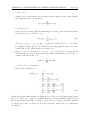
14 Phylogenetic Clustering (Phyloclustering)
14.1 Introduction . . . . . . . . . . . . . . . . . .
14.2 The phyclust Package . . . . . . . . . . . .
14.3 Bootstrap Method . . . . . . . . . . . . . .
14.4 Task Pull Parallelism . . . . . . . . . . . . .
14.5 An Example Using the Pony 524 Dataset .
14.6 Exercises . . . . . . . . . . . . . . . . . . .
.
.
.
.
.
.
.
.
.
.
.
.
.
.
.
.
.
.
.
.
.
.
.
.
.
.
.
.
.
.
.
.
.
.
.
.
.
.
.
.
.
.
.
.
.
.
.
.
.
.
.
.
.
.
.
.
.
.
.
.
.
.
.
.
.
.
.
.
.
.
.
.
.
.
.
.
.
.
.
.
.
.
.
.
.
.
.
.
.
.
.
.
.
.
.
.
.
.
.
.
.
.
.
.
.
.
.
.
.
.
.
.
.
.
.
.
.
.
.
.
.
.
.
.
.
.
103
103
105
106
107
109
110
15 Bayesian MCMC
15.1 Introduction . . . . . . . . . . . . . .
15.2 Hastings-Metropolis Algorithm . . .
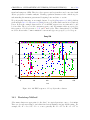
15.3 Galaxy Velocity . . . . . . . . . . . .
15.4 Parallel Random Number Generator
15.5 Exercises . . . . . . . . . . . . . . .
VI
.
.
.
.
.
.
.
.
.
.
.
.
.
.
.
.
.
.
.
.
.
.
.
.
.
.
.
.
.
.
.
.
.
.
.
.
.
.
.
.
.
.
.
.
.
.
.
.
.
.
Appendix
A Numerical Linear Algebra and Linear Least Squares
A.1 Forming the Normal Equations . . . . . . . . . . . . .
A.2 Using the QR Factorization . . . . . . . . . . . . . . .
A.3 Using the Singular Value Decomposition . . . . . . . .
.
.
.
.
.
.
.
.
.
.
.
.
.
.
.
.
.
.
.
.
.
.
.
.
.
.
.
.
.
.
.
.
.
.
.
.
.
.
.
.
.
.
.
.
.
.
.
.
.
.
.
.
.
.
.
.
.
.
.
.
.
.
.
.
.
.
.
.
.
.
.
.
.
.
.
111
111
112
114
115
116
118
Problems
119
. . . . . . . . . . . . . . . 119
. . . . . . . . . . . . . . . 120
. . . . . . . . . . . . . . . 121
B Linear Regression and Rank Degeneracy in R
122
VII
124
Miscellany
References
125
Index
130
List of Figures
1.1
1.2
1.3
pbdR Packages . . . . . . . . . . . . . . . . . . . . . . . . . . . . . . . . . . . . .
pbdR Package Use . . . . . . . . . . . . . . . . . . . . . . . . . . . . . . . . . . .
pbdR Interface to Foreign Libraries . . . . . . . . . . . . . . . . . . . . . . . . . .
4
4
5
2.1
2.2
Task Parallelism Example . . . . . . . . . . . . . . . . . . . . . . . . . . . . . . .
Task Parallelism Example . . . . . . . . . . . . . . . . . . . . . . . . . . . . . . .
11
13
4.1
Approximating π . . . . . . . . . . . . . . . . . . . . . . . . . . . . . . . . . . . .
35
5.1
5.2
Matrix Distribution Schemes . . . . . . . . . . . . . . . . . . . . . . . . . . . . .
Matrix Distribution Schemes Onto a 2-Dimensional Grid . . . . . . . . . . . . . .
43
44
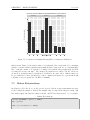
7.1
Covariance Benchmark . . . . . . . . . . . . . . . . . . . . . . . . . . . . . . . . .
62
10.1 Monthly averaged temperature . . . . . . . . . . . . . . . . . . . . . . . . . . . .
76
11.1 Matrix Redistribution Functions . . . . . . . . . . . . . . . . . . . . . . . . . . .
11.2 Load Balancing/Unbalancing Data . . . . . . . . . . . . . . . . . . . . . . . . . .
11.3 Converting Between GBD and DMAT . . . . . . . . . . . . . . . . . . . . . . . .
80
83
85
13.1
13.2
13.3
13.4
Iris
Iris
Iris
Iris
pair-wised scatter plot . .
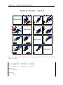
Clustering Plots — Serial
Clustering Plots — GBD
Clustering Plots — GBD
.
.
.
.
.
.
.
.
.
.
.
.
.
.
.
.
.
.
.
.
.
.
.
.
.
.
.
.
.
.
.
.
.
.
.
.
.
.
.
.
.
.
.
.
.
.
.
.
.
.
.
.
.
.
.
.
.
.
.
.
.
.
.
.
.
.
.
.
.
.
.
.
.
.
.
.
.
.
.
.
.
.
.
.
.
.
.
.
.
.
.
.
.
.
.
.
.
.
.
.
.
.
.
.
.
.
.
.
.
.
.
.
. 96
. 99
. 100
. 101
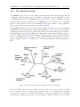
14.1 Retrovirus phylogeny originated from Weiss (2006). . . . . . . . . . . . . . . . . . 105
14.2 146 EIAV sequences of Pony 524 in three clusters. . . . . . . . . . . . . . . . . . 106
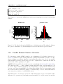
15.1 Histograms of velocities of 82 galaxies . . . . . . . . . . . . . . . . . . . . . . . . 114
15.2 MCMC results of velocities of 82 galaxies . . . . . . . . . . . . . . . . . . . . . . 115
List of Tables
3.1
Benchmark Comparing Rmpi and pbdMPI . . . . . . . . . . . . . . . . . . . . .
21
5.1
Processor Grid Shapes with 6 Processors . . . . . . . . . . . . . . . . . . . . . . .
45
10.1 Functions for accessing NetCDF4 files . . . . . . . . . . . . . . . . . . . . . . . .
75
11.1 Implicit Data Redistributions . . . . . . . . . . . . . . . . . . . . . . . . . . . . .
81
13.1 Parallel Mode-Based Clustering Algorithms in pmclust . . . . . . . . . . . . . . .
95
Acknowledgements
Schmidt, Ostrouchov, and Patel were supported in part by the project “NICS Remote Data
Analysis and Visualization Center” funded by the Office of Cyberinfrastructure of the U.S. National Science Foundation under Award No. ARRA-NSF-OCI-0906324 for NICS-RDAV center.
Chen was supported in part by the Department of Ecology and Evolutionary Biology at the
University of Tennessee, Knoxville, and a grant from the National Science Foundation (MCB1120370.)
Chen and Ostrouchov were supported in part by the project “Visual Data Exploration and
Analysis of Ultra-large Climate Data” funded by U.S. DOE Office of Science under Contract
No. DE-AC05-00OR22725.
This work used resources of National Institute for Computational Sciences at the University
of Tennessee, Knoxville, which is supported by the Office of Cyberinfrastructure of the U.S.
National Science Foundation under Award No. ARRA-NSF-OCI-0906324 for NICS-RDAV center. This work also used resources of the Oak Ridge Leadership Computing Facility at the Oak
Ridge National Laboratory, which is supported by the Office of Science of the U.S. Department
of Energy under Contract No. DE-AC05-00OR22725. This work used resources of the Newton
HPC Program at the University of Tennessee, Knoxville.
We also thank Brian D. Ripley, Kurt Hornik, Uwe Ligges, and Simon Urbanek from the R Core
Team for discussing package release issues and helping us solve portability problems on different
platforms.
Disclaimer
Warning: The findings and conclusions in this article have not been formally disseminated by
the U.S. Department of Energy and should not be construed to represent any determination or
policy of University, Agency and National Laboratory.
This document is written to explain the main functions of pbdDEMO (Schmidt et al., 2013), version . Every effort will be made to ensure future versions are consistent with these instructions,
but features in later versions may not be explained in this document.
Information about the functionality of this package, and any changes in future versions can be
found on website: “Programming with Big Data in R” at http://r-pbd.org/.
Part I
Preliminaries
1
Introduction
There are things which seem incredible to most
men who have not studied Mathematics.
—Archimedes of Syracus
1.1
What is pbdR?
The “Programming with Big Data in R” project (Ostrouchov et al., 2012) (pbdR for short) is
a project that aims to elevate the statistical programming language R (R Core Team, 2012b)
to leadership-class computing platforms. The main goal is empower data scientists by bringing
flexibility and a big analytics toolbox to big data challenges, with an emphasis on productivity,
portability, and performance. We achieve this in part by mapping high-level programming
syntax to portable, high-performance, scalable, parallel libraries. In short, we make R scalable.
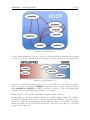
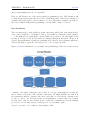
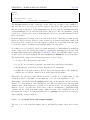
Figure 1.1 shows the current list of pbdR packages released to the CRAN (http://cran.
r-project.org), and how they depend on each other. More explicitly, the current pbdR
packages (Chen et al., 2012b,d; Schmidt et al., 2012a,b; Patel et al., 2013a; Schmidt et al., 2013)
are:
• pbdMPI — an efficient interface to MPI (Gropp et al., 1994) with a focus on Single
Program/Multiple Data (SPMD) parallel programming style.
• pbdSLAP — bundles scalable dense linear algebra libraries in double precision for R, based
on ScaLAPACK version 2.0.2 (Blackford et al., 1997).
• pbdNCDF4 — Interface to Parallel Unidata NetCDF4 format data files (NetCDF Group,
2008).
• pbdBASE — low-level ScaLAPACK codes and wrappers.
• pbdDMAT — distributed matrix classes and computational methods, with a focus on
linear algebra and statistics.
• pbdDEMO — set of package demonstrations and examples, and this unifying vignette.
CHAPTER 1. INTRODUCTION
4 of 132
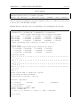
Figure 1.1: pbdR Packages
To try to make this landscape a bit more clear, one could divide pbdR packages into those meant
for users, developers, or something in-between. Figure 1.2 shows a gradient scale representation,
Figure 1.2: pbdR Package Use
where more red means the package is more for developers, while more blue means the package
is more for users. For example, pbdDEMO is squarely meant for users of pbdR packages,
while pbdBASE and pbdSLAP are really not meant for general use. The other packages fall
somewhere in-between, having plenty of utility for both camps.
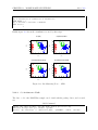
Finally, Figure 1.3 shows pbdR relationship to high-performance libraries.
In this vignette, we offer many examples using the above pbdR packages. Many of the examples
are high-level applications and may be commonly found in basic Statistics. The purpose is to
show how to reuse the preexisting functions and utilities of pbdR to create minor extensions
which can quickly solve problems in an efficient way. The reader is encouraged to reuse and
re-purpose these functions.
CHAPTER 1. INTRODUCTION
5 of 132
Figure 1.3: pbdR Interface to Foreign Libraries
The pbdDEMO package consists of two main parts. The first is a collection of roughly 20+
package demos. These offer example uses of the various pbdR packages. The second is this
vignette, which attempts to offer detailed explanations for the demos, as well as sometimes
providing some mathematical or statistical insight. A list of all of the package demos can be
found in Section 1.4.1.
1.2
Why Parallelism? Why pbdR?
It is common, in a document such as this, to justify the need for parallelism. Generally this
process goes:
Blah blah blah Moore’s Law, blah blah Big Data, blah blah blah Concurrency.
How about this? Parallelism is cool. Any boring nerd can use one computer, but using 10,000
at once is another story. We don’t call them supercomputers for nothing.
But unfortunately, lots of people who would otherwise be thrilled to do all kinds of cool stuff with
massive behemoths of computation — computers with names like KRAKEN1 and TITAN2 —
are burdened by an unfortunate reality: it’s really, really hard. Enter pbdR. Through our
project, we put a shiny new set of clothes on high-powered compiled code, making massive-scale
computation accessible to a wider audience of data scientists than ever before. Analytics in
supercomputing shouldn’t just be for the elites.
1.3
Installation
One can download pbdDEMO from CRAN at http://cran.r-project.org, and the installation can be done with the following commands
✞
tar zxvf pbdDEMO _ 0.2 -0. tar . gz
R CMD INSTALL pbdDEMO
✝
1
2
http://www.nics.tennessee.edu/computing-resources/kraken
http://www.olcf.ornl.gov/titan/
☎
✆
CHAPTER 1. INTRODUCTION
6 of 132
Since pbdEMO depends on other pbdR packages, please read the corresponding vignettes if
installation of any of them is unsuccessful.
1.4
Structure of pbdDEMO
The pbdDEMO package consists of several key components:
1. This vignette
2. A set of demos in the demo/ tree
3. A set of benchmark codes in the Benchmarks/ tree
The following subsections elaborate on the contents of the latter two.
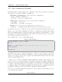
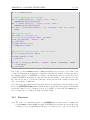
1.4.1
List of Demos
A full list of demos contained in the pbdDEMO package is provided below. We may or may not
describe all of the demos in this vignette.
List of Demos
✞
# ## ( Use Rscript . exe for windows systems )
# --------------------- #
# II Direct MPI Methods #
# --------------------- #
# ## Chapter 4
# Monte carlo
mpiexec - np 4
echo = F ) "
# Sample mean
mpiexec - np 4
echo = F ) "
# Binning
mpiexec - np 4
echo = F ) "
# Quantile
mpiexec - np 4
echo = F ) "
# OLS
mpiexec - np 4
# Distributed
mpiexec - np 4
echo = F ) "
simulation
Rscript -e " demo ( monte _ carlo , package = ’ pbdDMAT ’ , ask =F ,
and variance
Rscript -e " demo ( sample _ stat , package = ’ pbdDMAT ’ , ask =F ,
Rscript -e " demo ( binning , package = ’ pbdDMAT ’ , ask =F ,
Rscript -e " demo ( quantile , package = ’ pbdDMAT ’ , ask =F ,
Rscript -e " demo ( ols , package = ’ pbdDMAT ’ , ask =F , echo = F ) "
Logic
Rscript -e " demo ( comparators , package = ’ pbdDMAT ’ , ask =F ,
# ------------------------------ #
# III Distributed Matrix Methods #
# ------------------------------ #
☎
CHAPTER 1. INTRODUCTION
7 of 132
# ## Chapter 6
# Random matrix generation
mpiexec - np 4 Rscript -e " demo ( randmat _ global , package = ’ pbdDMAT ’ ,
ask =F , echo = F ) "
mpiexec - np 4 Rscript -e " demo ( randmat _ local , package = ’ pbdDMAT ’ , ask =F ,
echo = F ) "
# ## Chapter 8
# Sample statistics revisited
mpiexec - np 4 Rscript -e " demo ( sample _ stat _ dmat , package = ’ pbdDMAT ’ ,
ask =F , echo = F ) "
# Verify solving Ax = b at scale
mpiexec - np 4 Rscript -e " demo ( verify , package = ’ pbdDMAT ’ , ask =F ,
echo = F ) "
# PCA compression
mpiexec - np 4 Rscript -e " demo ( pca , package = ’ pbdDMAT ’ , ask =F , echo = F ) "
# OLS and predictions
mpiexec - np 4 Rscript -e " demo ( ols _ dmat , package = ’ pbdDMAT ’ , ask =F ,
echo = F ) "
# ---------------------------- #
# IV Reading and Managing Data #
# ---------------------------- #
# ## Chapter 9
# Reading csv
mpiexec - np 4 Rscript -e " demo ( read _ csv , package = ’ pbdDMAT ’ , ask =F ,
echo = F ) "
# Reading sql
mpiexec - np 4 Rscript -e " demo ( read _ sql , package = ’ pbdDMAT ’ , ask =F ,
echo = F ) "
# ## Chapter 10
# Reading and writing parallel NetCDF4
Rscript -e " demo ( trefht , package = " pbdDEMO " , ask = F , echo = F ) "
mpiexec - np 4 Rscript -e " demo ( nc4 _ serial , package = ’ pbdDEMO ’ , ask =F ,
echo = F ) "
mpiexec - np 4 Rscript -e " demo ( nc4 _ parallel , package = ’ pbdDEMO ’ , ask =F ,
echo = F ) "
mpiexec - np 4 Rscript -e " demo ( nc4 _ dmat , package = ’ pbdDEMO ’ , ask =F ,
echo = F ) "
mpiexec - np 4 Rscript -e " demo ( nc4 _ gbdc , package = ’ pbdDEMO ’ , ask =F ,
echo = F ) "
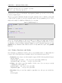
# ## Chapter 11
# Loand / unload balance
mpiexec - np 4 Rscript -e " demo ( balance , package = ’ pbdDMAT ’ , ask =F ,
echo = F ) "
# GBD to DMAT
mpiexec - np 4 Rscript -e " demo ( gbd _ dmat , package = ’ pbdDMAT ’ , ask =F ,
echo = F ) "
# Distributed matrix redistributions
CHAPTER 1. INTRODUCTION
8 of 132
mpiexec - np 4 Rscript -e " demo ( reblock , package = ’ pbdDMAT ’ , ask =F ,
echo = F ) "
# ---------------------------- #
# V Applications
#
# ---------------------------- #
# ## Chapter 13
# Parallel Model - Based Clustering
Rscript -e " demo ( iris _ overlap , package = ’ pbdDEMO ’ , ask =F , echo = F ) "
Rscript -e " demo ( iris _ serial , package = ’ pbdDEMO ’ , ask =F , echo = F ) "
Rscript -e " demo ( iris _ gbd , package = ’ pbdDEMO ’ , ask =F , echo = F ) "
Rscript -e " demo ( iris _ dmat , package = ’ pbdDEMO ’ , ask =F , echo = F ) "
# ## Chapter 14
mpiexec - np 4 Rscript -e " demo ( task _ pull , package = ’ pbdMPI ’ , ask =F ,
echo = F ) "
mpiexec - np 4 Rscript -e " demo ( phyclust _ bootstrap , package = ’ pbdDEMO ’ ,
ask =F , echo = F ) "
# ## Chapter 15
mpiexec - np 4 Rscript -e " demo ( mcmc _ galaxy , package = ’ pbdDEMO ’ , ask =F ,
echo = F ) "
✝
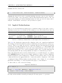
1.4.2
✆
List of Benchmarks
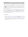
At the time of writing, there are benchmarks for computing covariance, linear models, and
principal components. The benchmarks come in two variants. The first is an ordinary set of
benchmark codes, which generate data of specified dimension(s) and time the indicated computation. This operation is replicated for a user-specified number of times (default 10), and then
the timing results are printed to the terminal.
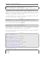
From the Benchmarks/ subtree, the user can run the first set of benchmarks with, for example,
4 processors by issuing any of the commands:
✞
# ## ( Use Rscript . exe for windows systems )
mpiexec - np 4 Rscript cov . r
mpiexec - np 4 Rscript lmfit . r
mpiexec - np 4 Rscript pca . r
✝
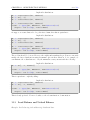
The second set of benchmarks are those that try to find the “balancing” point where, for the
indicted computation with user specified number of cores, the computation is performed faster
using pbdR than using serial R. In general, throwing a bunch of cores at a problem may not be
the best course of action, because parallel algorithms (almost always) have inherent overhead
over their serial counterparts that can make their use ill-advised for small problems. But for
sufficiently big (which is usually not very big at all) problems, that overhead should quickly be
dwarfed by the increased scalability.
From the Benchmarks/ subtree, the user can run the second set of benchmarks with, for example,
☎
✆
CHAPTER 1. INTRODUCTION
9 of 132
4 processors by issuing any of the commands:
✞
# ## ( Use Rscript . exe for windows systems )
mpiexec - np 4 Rscript balance _ cov . r
mpiexec - np 4 Rscript balance _ lmfit . r
mpiexec - np 4 Rscript balance _ pca . r
✝
☎
✆
Now we must note that there are other costs than just statistical computation. There is of course
the cost of disk IO (when dealing with real data). However, a parallel file system should help
with this, and for large datasets should actually be faster anyway. The main cost not measured
here is the cost of starting all of the R processes and loading packages. Assuming R is not
compiled statically (and it almost certainly is not), then this cost is non-trivial and somewhat
unique to very large scale computing. For instance, it took us well over an hour to start 12,000
R sessions and load the required packages on the supercomputer KRAKEN3 . This problem is
not unique to R, however. It affects any project that has a great deal of dynamic library loading
to do. This includes Python, although their community has made some impressive strides in
dealing with this problem.
1.5
Exercises
1-1 Read the MPI wikipedia page https://en.wikipedia.org/wiki/Message_Passing_Interface
including it’s history, overview, functionality, and concepts sections.
1-2 Read the pbdMPI vignette and install either OpenMPI (http://www.open-mpi.org/)
or MPICH2 (http://www.mcs.anl.gov/research/projects/mpich2/), and test if the
installation is correct (see http://www.r-pbd.org/install.html for more details).
1-3 After completing Exercise 1-2, install all pbdR packages and run each package’s demo
codes.
3
See https://en.wikipedia.org/wiki/Kraken_(supercomputer)
2
Background
We stand at the threshold of a many core world.
The hardware community is ready to cross this
threshold. The parallel software community is
not.
—Tim Mattson
2.1
Parallelism
What is parallelism? At its core (pun intended), parallelism is all about trying to throw more
resources at a problem, usually to get the problem to complete faster than it would with the more
minimal resources. Sometimes we wish to utilize more resources as a means of being able to make
a computationally (literally or practically) intractable problem into one which will complete in
a reasonable amount of time. Somewhat more precisely, parallelism is the leveraging of parallel
processing. It is a general programming model whereby we execute different computations
simultaneously. This stands in contrast to serial programming, where you have a stream of
commands, executed one at a time.
Serial programming has been the dominant model from the invention of the computer to present,
although this is quickly changing. The reasons why this is changing are numerous and boring;
the fact is, if it is true now that a researcher must know some level of programming to do his/her
job, then it is certainly true that in the near future that he/she will have to be able to do some
parallel programming. Anyone who would deny this is, frankly, more likely trying to vocally
assuage personal fears more so than accurately forecasting based on empirical evidence. For
many, parallel programming isn’t coming; it’s here.
As a general rule, parallelism should only come after you have exhausted serial optimization.
Even the most complicated parallel programs are made up of serial pieces, so inefficient serial
codes produce inefficient parallel codes. Also, generally speaking, one can often eke out much
better performance by implementing a very efficient serial algorithm rather than using a handful
of cores (like on a modern multicore laptop) using an inefficient parallel algorithm. However,
once that serial-optimization well runs dry, if you want to continue seeing performance gains,
CHAPTER 2. BACKGROUND
11 of 132
then you must implement your code in parallel.
Next, we will discuss some of the major parallel programming models. This discussion will
be fairly abstract and superficial; however, the overwhelming bulk of this text is comprised of
examples which will appeal to data scientists, so for more substantive examples, especially for
those more familiar with parallel programming, you may wish to jump to Section 4.
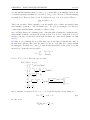
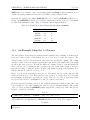
Data Parallelism
There are many ways to write parallel programs. Often these will depend on the physical hardware you have available to you (multicore laptop, several GPU’s, a distributed supercomputer,
. . . ). The pbdR project is principally concerned with data parallelism. We will expand on the
specifics in Section 2.3 and provide numerous examples throughout this guide. However, in
general, data parallelism is a parallel programming model whereby the programmer splits up a
data set and applies operations on the sub-pieces to solve one larger problem.
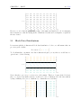
Figure 2.1 offers a visualization of a very simple data parallelism problem. Say we have an array
Figure 2.1: Task Parallelism Example
consisting of the values 1 through 8, and we have 4 cores (processing units) at our disposal,
and we want to add up all of the elements of this array. We might distribute the data as in
the diagram (the first two elements of the array on the first core, the next two elements on the
second core, and so on). We then perform a local summation operation; this local operation
is serial, but because we have divided up the overall task of summation across the multiple
processors, for a very large array we would expect to see performance gains.
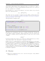
A very loose pseudo code for this procedure might look like:
CHAPTER 2. BACKGROUND
12 of 132
Pseudocode
1:
2:
3:
4:
5:
6:
mydata = map(data)
total local = sum(mydata)
total = reduce(total local)
if this processor == processor 1 then
print(total)
end if
Then each of the four cores could execute this code simultaneously, with some cooperation
between the processors for step 1 (in determining who owns what) and for the reduction in
step 3. This is an example of using a higher-level parallel programming paradigm called “Single
Program/Multiple Data” or SPMD. . We will elucidate more as to exactly what this means in
the sections to follow.
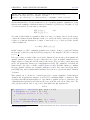
Task Parallelism
Data parallelism is one parallel programming model. By contrast, another important parallel
programming model is task parallelism, which much of the R community is already fairly adept
at, especially when using the manager/workers paradigm (more on this later). Common packages
for this kind of work include snow (Tierney et al., 2012), parallel (R Core Team, 2012a), and
Rmpi (Yu, 2002)1 .
Task parallelism involves, as the name implies, distributing different execution tasks across processors. Task parallelism is often embarrassingly parallel — meaning the parallelism is so easy
to exploit that it is embarrassing. This kind of situation occurs when you have complete independence, or a loosely coupled problem (as opposed to something tightly coupled, like computing
the singular value decomposition (SVD) of a distributed data matrix, for example).
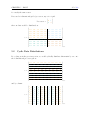
As a simple example of task parallelism, say you have one dataset and four processing cores, and
you want to fit all four different linear regression models for that dataset, and then choose the
model with lowest AIC (Akaike, 1974) (we are not arguing that this is necessarily a good idea;
this is just an example). Fitting one model does not have any dependence on fitting another, so
you might want to just do the obvious thing and have each core fit a separate model, compute
the AIC value locally, then compare all computed AIC values, lowest is the winner. Figure 2.2
offers a simple visualization of this procedure.
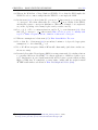
A very loose pseudo code for this problem might look like:
Pseudocode
1
For more examples, see “CRAN Task View: High-Performance and Parallel Computing with R” at http:
//cran.r-project.org/web/views/HighPerformanceComputing.html.
CHAPTER 2. BACKGROUND
13 of 132
Figure 2.2: Task Parallelism Example
1:
2:
3:
4:
5:
6:
7:
8:
9:
10:
11:
load data()
if this processor == processor 1 then
distribute tasks()
else
receive tasks()
end if
model aic = aic(fit(mymodel))
best aic = min(allgather(model aic))
if model aic == best aic then
print(mymodel)
end if
Then each of the four cores could execute this code simultaneously, with some cooperation
between the processors for the distribution of tasks (which model to fit) in step 2 and for the
gather operation in step 8.
The line between data parallelism and task parallelism sometimes blurs, especially in simple
examples such as those presented here; given our loose definitions of terms, is our first example
really data parallelism? Or is it task parallelism? It is best not to spend too much time
worrying about what to call it and instead focus on how to do it. These are simple examples
and should not be taken too far out of context. All that said, the proverbial rabbit hole of
parallel programming goes quite deep, and often it is not a matter of one programming model
or another, but leveraging several at once to solve a complicated problem.
CHAPTER 2. BACKGROUND
2.2
14 of 132
SPMD Programming with R
Throughout this document, we will be using the ‘Single Program/Multiple Data”, or SPMD,
paradigm for distributed computing. Writing programs in the SPMD style is a very natural
way of doing computations in parallel, but can be somewhat difficult to properly describe. As
the name implies, only one program is written, but the different processors involved in the
computation all execute the code independently on different portions of the data. The process
is arguably the most natural extension of running serial codes in batch. This model lends itself
especially well to data parallelism problems.
Unfortunately, executing jobs in batch is a somewhat unknown way of doing business to the
typical R user. While details and examples about this process will be provided in the chapters
to follow, the reader is encouraged to read the pbdMPI package’s vignette (Chen et al., 2012c)
first. Ideally, readers should run the demos of the pbdMPI package, going through the code
step by step.
This paradigm is just one model of parallel programming, and in reality, is a sort of “meta
model”, encompassing many other parallel programming models. The R community is already
familiar with the manager/workers2 programming model. This programming model is particularly well-suited to task parallelism, where generally one processor will distribute the task load
to the other processors.
The two are not mutually exclusive, however. It is easy enough to engage in task parallelism
from an SPMD-written program. To do this, you essentially create a “task-parallelism block”,
where one processor
Pseudocode
if this processor == manager then
distribute tasks()
3: else
4:
receive tasks()
5: end if
1:
2:
See Exercise 2-2 for more details.
One other model of note is the MapReduce model. A well-known implementation of this is
Apache’s Hadoop, which is really more of a poor man’s distributed file system with MapReduce
bolted on top. The R community has a strange affection for MapReduce, even among people
who have never used it. MapReduce, and for instance Hadoop, most certainly has its place,
but one should be aware that MapReduce is not very well-suited for tightly coupled problems;
this difficulty goes beyond the fact that tightly coupled problems are harder to parallelize than
their embarrassingly parallel counterparts, and is, in part, inherent to MapReduce itself. For
the remainder of this document, we will not discuss MapReduce further.
2
Sometimes referred to as “master/slaves” or “master/workers”
CHAPTER 2. BACKGROUND
2.3
15 of 132
Notation
Note that we tend to use suffix .gbd for an object when we wish to indicate that the object
is “general block distributed.” This is purely for pedagogical convenience, and has no semantic
meaning. Since the code is written in SPMD style, you can think of such objects as referring to
either a large, global object, or to a processor’s local piece of the whole (depending on context).
This is less confusing than it might first sound.
We will not use this suffix to denote a global object common to all processors. As a simple
example, you could imagine having a large matrix with (global) dimensions m × n with each
processor owning different collections of rows of the matrix. All processors might need to know
the values for m and n; however, m and n do not depend on the local process, and so these do
not receive the .gbd suffix. In many cases, it may be a good idea to invent an S4 class object
and a corresponding set of methods. Doing so can greatly improve the usability and readability
of your code, but is never strictly necessary. However, these constructions are the foundation of
the pbdBASE (Schmidt et al., 2012a) and pbdDMAT (Schmidt et al., 2012b) packages.
On that note, depending on your requirements in distributed computing with R, it may be beneficial to you to use higher pbdR toolchain. If you need to perform dense matrix operations,
or statistical analysis which depend heavily on matrix algebra (linear modeling, principal components analysis, . . . ), then the pbdBASE and pbdDMAT packages are a natural choice. The
major hurdle to using these tools is getting the data into the appropriate ddmatrix format, although we provide many tools to ease the pains of doing so. Learning how to use these packages
can greatly improve code performance, and take your statistical modeling in R to previously
unimaginable scales.
Again for the sake of understanding, we will at times append the suffix .dmat to objects of class
ddmatrix to differentiate them from the more general .gbd object. As with .gbd, this carries
no semantic meaning, and is merely used to improve the readability of example code (especially
when managing both “.gbd” and ddmatrix objects).
2.4
Exercises
2-1 Read the SPMD wiki page at http://en.wikipedia.org/wiki/SPMD and it’s related information.
2-2 pbdMPI provides a function get.jid() to divide N jobs into n processors nearly equally
which is best for homogeneous computing environment to do task parallelism. The FAQs
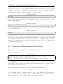
section of pbdMPI’s vignette has an example, try it as next.
✞
1
2
library ( pbdMPI , quiet = TRUE )
init ()
3
4
5
id <- get . jid ( N )
R Code
☎
CHAPTER 2. BACKGROUND
6
7
8
9
10
16 of 132
# ## Using a loop
for ( i in id ) {
# put independent task i script here
}
finalize ()
✝
See Section 14.4 for more efficient task parallelism.
2-3 Multi-threading and forking are also popular methods of parallelism for shared memory
systems, such as in a personal laptop. The function mclapply()3 in parallel originated
from the multicore (Urbanek, 2011) package, and is for simple parallelism on shared memory machines by using the fork mechanism. Compare this with OpenMP (OpenMP ARB,
1997).
3
This method is not available on Windows, because Windows has no system-level fork command.
✆
Part II
Direct MPI Methods
3
MPI for the R User
Everybody who learns concurrency thinks they
understand it, ends up finding mysterious races
they thought weren’t possible, and discovers that
they didn’t actually understand it yet after all.
—Herb Sutter
Cicero once said that “If you have a garden and a library, you have everything you need.” So
in that spirit, for the next two chapters we will use the MPI library to get our hands dirty and
root around in the dirt of low-level MPI programming.
3.1
MPI Basics
In a sense, Cicero (in the above tortured metaphor) was quite right. MPI is all that we need in
the same way that I might only need bread and cheese, but really what I want is a pizza. MPI
is somewhat low-level and can be quite fiddly, but mastering it adds a very powerful tool to the
repertoire of the parallel R programmer, and is essential for anyone who wants to do large scale
development of parallel codes.
“MPI” stands for “Message Passing Interface”. How it really works goes well beyond the scope
of this document. But at a basic level, the idea is that the user is running a code on different
compute nodes that (usually) can not directly modify objects in each others’ memory. In order
to have all of the nodes working together on a common problem, data and computation directives
are passed around over the network (often over a specialized link called infiniband).
At its core, MPI is a standard interface for managing communications (data and instructions)
between different nodes or computers. There are several major implementations of this standard,
and the one you should use may depend on the machine you are using. But this is a compiling
issue, so user programs are unaffected beyond this minor hurdle. Some of the most well-known
implementations are OpenMPI, MPICH2, and Cray MPT.
CHAPTER 3. MPI FOR THE R USER
19 of 132
At the core of using MPI is the communicator. At a technical level, a communicator is a pretty
complicated data structure, but these deep technical details are not necessary for proceeding.
We will instead think of it somewhat like the post office. When we wish to send a letter
(communication) to someone else (another processor), we merely drop the letter off at a post
office mailbox (communicator) and trust that the post office (MPI) will handle things accordingly
(sort of).
The general process for directly — or indirectly — utilizing MPI in SPMD programs goes
something like this:
1. Initialize communicator(s).
2. Have each process read in its portion of the data.
3. Perform computations.
4. Communicate results.
5. Shut down the communicator(s).
Some of the above steps may be swept away under a layer of abstraction for the user, but the
need may arise where directly interfacing with MPI is not only beneficial, but necessary.
More details and numerous examples using MPI with R are available in the sections to follow,
as well as in the pbdMPI vignette.
3.2
pbdMPI vs Rmpi
There is another package on the CRAN which the R programmer may use to interface with
MPI, namely Rmpi (Yu, 2002). There are several issues one must consider when choosing which
package to use if one were to only use one of them.
1. (+) pbdMPI is easier to install than Rmpi
2. (+) pbdMPI is easier to use than Rmpi
3. (+) pbdMPI can often outperform Rmpi
4. (+) pbdMPI integrates with the rest of pbdR
5. (−) Rmpi can be used with foreach (Analytics, 2012) via doMPI (Weston, 2010)
6. (−) Rmpi can be used in the manager/worker paradigm
We do not believe that the above can be reduced to a zero-sum game with unambiguous winner
and loser. Ultimately the needs of the user (or developer) are paramount. We believe that
pbdR makes a very good case for itself, especially in the SPMD style, but it can not satisfy
everyone. However, for the remainder of this section, we will present the case for several of the,
as yet, unsubstantiated pluses above.
CHAPTER 3. MPI FOR THE R USER
20 of 132
In the case of ease of use, Rmpi uses bindings very close to the level as they are used in C’s MPI
API. Specifically, whenever performing, for example, a reduction operation such as “allreduce”,
you must specify the type of your data. For example, using Rmpi’s API
✞
1
☎
mpi . allreduce (x , type = 1)
✝
✆
would perform the sum allreduce if the object x consists of integer data, while
✞
1
☎
mpi . allreduce (x , type = 2)
✝
✆
would be used if x consists of doubles. However, with pbdMPI
✞
1
☎
allreduce ( x )
✝
✆
is used for both by making use of R’s S4 system of object oriented programming. This is not
mere code golfing1 that we are engaging in. The concept of what “type” your data is in R is
fairly foreign to most R users, and misusing the type argument in Rmpi is a very easy way to
crash your program. Even if you are more comfortable with statically typed languages and have
no problem with this concept, consider the following example:
Types in R
✞
1
2
3
4
5
6
☎
> is . integer (1)
[1] FALSE
> is . integer (2)
[1] FALSE
> is . integer (1:2)
[1] TRUE
✝
✆
There are good reasons for R Core to have made this choice; that is not the point. The point
is that because objects in R are dynamically typed, having to know the type of your data when
utilizing Rmpi is a needless burden. Instead, pbdMPI takes the approach of adding a small
abstraction layer on top (which we intend to show does not negatively impact performance) so
that the user need not worry about such fiddly details.
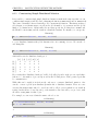
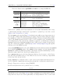
In terms of performance, pbdMPI can greatly outperform Rmpi. We present here the results of a benchmark we performed comparing the “allgather” operation between the two packages (Schmidt et al., 2012e). The benchmark consisted of calling the respective “allgather”
function from each package on a randomly generated 10, 000 × 10, 000 distributed matrix with
entries coming from the standard normal distribution, using different numbers of processors.
Table 3.1 shows the results for this test, and in each case, pbdMPI is the clear victor.
Whichever package you choose, whichever your favorite, for the remainder of this document we
will be using (either implicitly or explicitly) pbdMPI.
1
See https://en.wikipedia.org/wiki/Code_golf
CHAPTER 3. MPI FOR THE R USER
21 of 132
Table 3.1: Benchmark Comparing Rmpi and pbdMPI. Run time in seconds is listed for each
operation. The speedup is relative to Rmpi.
Cores
32
64
128
256
3.3
Rmpi
24.6
25.2
22.3
22.4
pbdMPI
6.7
7.1
7.2
7.1
Speedup
3.67
3.55
3.10
3.15
The GBD Data Structure
This is the boring stuff everyone hates, but like your medicine, it’s ultimately better for you to
just take it and get it out of the way: data structures. In particular, we will be discussing a
distributed data structure that, for lack of a better name (and I assure you are tried), we will
call the GBD data structure. This data structure is more paradigm or philosophy than a rigid
data structure like an array or list. Consider it a set of “best practices”, or if nothing else, a
starting place if you have no idea how to proceed.
The GBD data structure is designed to fit the types of problems which are arguably most
common to data science, namely tall and skinny matrices. It will work best with these (from
a computational efficiency perspective) problems, although that is not required. In fact, very
little at all is required of this data structure. At its core, the data structure is a distributed
matrix data structure, with the following rules:
1. GBD is distributed. No one processor owns all of the matrix.
2. GBD is non-overlapping. Any row owned by one processor is owned by no other processors.
3. GBD is row-contiguous. If a processor owns one element of a row, it owns the entire row.
4. GBD is globally row-major 2 , locally column-major 3 .
5. The last row of the local storage of a processor is adjacent (by global row) to the first row
of the local storage of next processor (by communicator number) that owns data. That is,
global row-adjacency is preserved in local storage via the communicator.
6. GBD is (relatively) easy to understand, but can lead to bottlenecks if you have many more
columns than rows.
Of this list, perhaps the most difficult to understand is number 5. This is a precise, albeit
cumbersome explanation for a simple idea. If two processors are adjacent and each owns data,
then their local sub-matrices are adjacent row-wise as well. For example, rows n and n + 1 of a
matrix are adjacent; possible configurations for the distributed ownership are processors q owns
row n and q + 1 owns row n + 1; processor q owns row n, processor q + 1 owns nothing, and
processor q + 2 owns row n + 1.
2
In the sense of the data decomposition. More specifically, the global matrix is chopped up into local submatrices in a row-major way.
3
The local sub-objects are R matrices, which are stored in column-major fashion.
CHAPTER 3. MPI FOR THE R USER
22 of 132
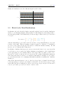
For some, no matter how much we try or what we write, the wall of text simply will not suffice.
So here are a few visual examples. Suppose we have the global data matrix x, given as:
x=
x11
x21
x31
x41
x51
x61
x71
x81
x91
x12
x22
x32
x42
x52
x62
x72
x82
x92
x13
x23
x33
x43
x53
x63
x73
x83
x93
x14
x24
x34
x44
x54
x64
x74
x84
x94
x15
x25
x35
x45
x55
x65
x75
x85
x95
x16
x26
x36
x46
x56
x66
x76
x86
x96
x17
x27
x37
x47
x57
x67
x77
x87
x97
x18
x28
x38
x48
x58
x68
x78
x88
x98
x19
x29
x39
x49
x59
x69
x79
x89
x99
9×9
with processor array4 (indexing always starts at 0 not 1)
Processors = 0 1 2 3 4 5
Then we might split up and distribute the data onto processors like so:
x=
x11
x21
x31
x41
x51
x61
x71
x81
x91
x12
x22
x32
x42
x52
x62
x72
x82
x92
x13
x23
x33
x43
x53
x63
x73
x83
x93
x14
x24
x34
x44
x54
x64
x74
x84
x94
x15
x25
x35
x45
x55
x65
x75
x85
x95
x16
x26
x36
x46
x56
x66
x76
x86
x96
x17
x27
x37
x47
x57
x67
x77
x87
x97
x18
x28
x38
x48
x58
x68
x78
x88
x98
x19
x29
x39
x49
x59
x69
x79
x89
x99
9×9
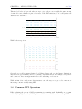
With local storage view:
"
"
"
h
h
4
h
x11 x12 x13 x14 x15 x16 x17 x18 x19
x21 x22 x23 x24 x25 x26 x27 x28 x29
#
2×9
x31 x32 x33 x34 x35 x36 x37 x38 x39
x41 x42 x43 x44 x45 x46 x47 x48 x49
#
2×9
x51 x52 x53 x54 x55 x56 x57 x58 x59
x61 x62 x63 x64 x65 x66 x67 x68 x69
#
2×9
x71 x72 x73 x74 x75 x76 x77 x78 x79
i
x81 x82 x83 x84 x85 x86 x87 x88 x89
x91 x92 x93 x94 x95 x96 x97 x98 x99
i
i
1×9
1×9
1×9
Palette selected to be distinguishable by the color blind, taken from http://jfly.iam.u-tokyo.ac.jp/color/
#pallet
CHAPTER 3. MPI FOR THE R USER
23 of 132
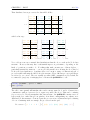
This is a load balanced approach, where we try to give each processor roughly the same amount
of stuff. Of course, that is not part of the rules of the GBD structure, so we could just as well
distribute the data like so:
x=
x11
x21
x31
x41
x51
x61
x71
x12
x22
x32
x42
x52
x62
x72
x13
x23
x33
x43
x53
x63
x73
x14
x24
x34
x44
x54
x64
x74
x15
x25
x35
x45
x55
x65
x75
x16
x26
x36
x46
x56
x66
x76
x17
x27
x37
x47
x57
x67
x77
x18
x28
x38
x48
x58
x68
x78
x19
x29
x39
x49
x59
x69
x79
x89
x81 x82 x83 x84 x85 x86 x87 x88
x91 x92 x93 x94 x95 x96 x97 x98 x99
9×9
With local storage view:
h
0×9
x19
x29
x39
x49
x51 x52 x53 x54 x55 x56 x57 x58 x59
x61 x62 x63 x64 x65 x66 x67 x68 x69
#
x11 x12
x22
x32
x41 x42
x
21
x31
"
h
h
"
i
x13
x23
x33
x43
x14
x24
x34
x44
x15
x25
x35
x45
x16
x26
x36
x46
x17
x27
x37
x47
x18
x28
x38
x48
x71 x72 x73 x74 x75 x76 x77 x78 x79
4×9
i
2×9
1×9
i
0×9
x81 x82 x83 x84 x85 x86 x87 x88 x89
x91 x92 x93 x94 x95 x96 x97 x98 x99
#
2×9
Generally, we would recommend using a load balanced approach over this bizarre distribution,
although some problems may call for very strange data distributions. For example, it is possible
and common to have an empty matrix after some subsetting or selectation.
With our first of two cumbersome data structures out of the way, we can proceed to much more
interesting content: actually using MPI.
3.4
Common MPI Operations
Fully explaining the process of MPI programming is a daunting task. Thankfully, we can punt
and merely highlight some key MPI operations and how one should use them with pbdMPI.
CHAPTER 3. MPI FOR THE R USER
3.4.1
24 of 132
Basic Communicator Wrangling
First things first, we must examine basic communicator issues, like construction, destruction,
and each processor’s position within a communicator.
• Managing a Communicator: Create and destroy communicators.
init() — initialize communicator
finalize() — shut down communicator(s)
• Rank query: Determine the processor’s position in the communicator.
comm.rank() — “who am I?”
comm.size() — “how many of us are there?”
• Barrier: No processor can proceed until all processors can proceed.
barrier() — “computation wall” that only all processors together can tear down.
One quick word before proceeding. If a processor queries comm.size(), this will return the total
number of processors in the communicators. However, communicator indexing is like indexing
in the programming language C. That is, the first element is numbered 0 rather than 1. So when
the first processor queries comm.rank(), it will return 0, and when the last processor queries
comm.rank(), it will return comm.size() - 1.
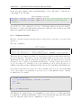
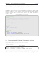
We are finally ready to write our first MPI program:
✞
1
2
Simple pbdMPI Example 1
☎
library ( pbdMPI , quiet = TRUE )
init ()
3
4
5
myRank <- comm . rank () + 1 # comm index starts at 0 , not 1
print ( myRank )
6
7
finalize ()
✝
✆
Unfortunately, it is not very exciting, but you have to crawl before you can drag race. Remember
that all of our programs are written in SPMD style. So this one single program is written, and
each processor will execute the same program, but with different results, whence the name
“Single Program/Multiple Data”.
So what does it do? First we initialize the MPI communicator with the call to init(). Next,
we have each processor query its rank via comm.rank(). Since indexing of MPI communicators
starts at 0, we add 1 because that is what we felt like doing. Finally we call R’s print() function
to print the result. This printing is not particularly clever, and each processor will be clamoring
to dump its result to the output file/terminal. We will discuss more sophisticated means of
printing later. Finally, we shut down the MPI communicator with finalize().
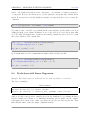
If you were to save this program in the file mpiex1.r and you wished to run it with 2 processors,
you would issue the command:
✞
Shell Command
☎
CHAPTER 3. MPI FOR THE R USER
25 of 132
# ## ( Use Rscript . exe for windows system )
mpiexec - np 2 Rscript mpiex1 . r
✝
✆
To use more processors, you modify the -np argument (“number processors”). So if you want
to use 4, you pass -np 4.
The above program technically, though not in spirit, bucks the trend of officially opening with
a “Hello World” program. So as not to incur the wrath of the programming gods, we offer a
simple such example by slightly modifying the above program:
Simple pbdMPI Example 1.5
✞
1
2
☎
library ( pbdMPI , quiet = TRUE )
init ()
3
4
myRank <- comm . rank ()
5
6
7
8
if ( myRank == 0) {
print ( " Hello , world . " )
}
9
10
finalize ()
✝
✆
One word of general warning we offer now is that we are taking very simple approaches here
for the sake of understanding, heavily relying on function argument defaults. However, there
are all kinds of crazy, needlessly complicated things you can do with these functions. See the
pbdMPI reference manual for full details about how one may utilize these (and other) pbdMPI
functions.
3.4.2
Reduce, Broadcast, and Gather
Once managing a communicator is under control, you presumably want to do things with all of
your processors. The typical way you will have the processors interact is given below:
• Reduction: Say each processor has a number x.gbd. Add all of them up, find the largest,
find the smallest, . . . .
reduce(x.gbd, op=’sum’) — only one processor gets result (default is 0)
allreduce(x.gbd, op=’sum’) — every processor gets result
• Gather: Say each processor has a number. Create a new object on some processor(s)
containing all of those numbers.
gather(x.gbd) — only one processor gets result
allgather(x.gbd) — every processor gets result
• Broadcast: One processor has a number x.gbd that every other processor should also
have.
bcast(x.gbd)
CHAPTER 3. MPI FOR THE R USER
26 of 132
Here perhaps explanations are inferior to examples; so without wasting any more time, we
proceed to the next example:
Simple pbdMPI Example 2
✞
1
2
☎
library ( pbdMPI , quiet = TRUE )
init ()
3
4
n . gbd <- sample (1:10 , size =1)
5
6
7
sm <- allreduce ( n . gbd ) # default op is ’sum ’
print ( sm )
8
9
10
gt <- allgather ( n . gbd )
print ( gt )
11
12
finalize ()
✝
✆
So what does it do? First each processor samples a number from 1 to 10; it is probably true
that each processor will be using a different seed for this sampling, though you should not rely
on this alone to ensure good parallel seeds. More on this particular problem in Section 3.4.3
below.
Next, we perform an allreduce() on n.gbd. Conceivably, the processors could have different
values for n.gbd. So the value of n is local to each processor. So perhaps we want to add up
all these numbers (with as many numbers as there are processors) and store them in the global
value sm (for “sum”). Each processor will agree as to the value of sm, even if they disagree about
the value of n.gbd.
Finally, we do the same but with an allgather() operation.
Try experimenting with this by running the program several times. You should get different
results each time. To make sure we have not been lying to you about what is happening, you
can even print the values of n.gbd before the reduce and gather operations.
3.4.3
Printing and RNG Seeds
In addition to the above common MPI operations, which will make up the bulk of the MPI
programmer’s toolbox, we offer a few extra utility functions:
• Print: printing with control over which processor prints.
comm.print(x, ...)
comm.cat(x, ...)
• Random Seeds:
comm.set.seed(seed, diff=FALSE): every processor uses the seed seed
comm.set.seed(diff=TRUE): every processor uses an independent seed (via rlecuyer)
CHAPTER 3. MPI FOR THE R USER
27 of 132
The comm.print() and comm.cat() functions are especially handy, because they are much more
sophisticated than their R counterparts when using multiple processes. These functions which
processes do the printing, and if you choose to have all processes print their result, then the
printing occurs in an orderly fashion, with processor 0 getting the first line, processor 1 getting
the second, and so on.
For example, revisiting our “Hello, world” example, we can somewhat simplify the code with a
slight modification:
Simple pbdMPI Example 3
✞
1
2
☎
library ( pbdMPI , quiet = TRUE )
init ()
3
4
myRank <- comm . rank ()
5
6
comm . print ( " Hello , world . " )
7
8
finalize ()
✝
✆
If we want to see what each processor has to say, we can pass the optional argument all,rank=TRUE
to comm.print(). By default, each process will print its rank, then what you told it to print.
You can suppress the printing of communicator rank via the optional argument quiet=TRUE to
comm.print().
These functions are quite handy. . .
##### HOWEVER #####
these functions are potentially dangerous, and so some degree of care should be exercised. Indeed,
it is possible to lock up all of the active R sessions by incorrectly using them. Worse, achieving
this behavior is fairly easy to do. The way this occurs is by issuing a comm.print() on an
expression which requires communication. For example, suppose we have a distributed object
with local piece x.gbd and a function myFunction() which requires communication between the
processors. Then calling
✞
1
A Cautionary Tale of Printing in Parallel (1 of 3)
☎
print ( myFunction ( x . gbd ) )
✝
✆
is just fine, but will not have the nice orderly, behaved printing style of comm.print(). However,
if we issue
✞
1
A Cautionary Tale of Printing in Parallel (2 of 3)
☎
comm . print ( myFunction ( x . gbd ) )
✝
then we have just locked up all of the R processes. Indeed, behind the scenes, a call somewhat
akin to
✆
CHAPTER 3. MPI FOR THE R USER
28 of 132
✞
1
2
3
4
5
6
☎
for ( rank in 0: comm . size () ) {
if ( comm . rank () == rank ) {
# do things
}
barrier ()
}
✝
✆
has been ordered. The problem arises in the “do things” part. Since (in our hypothetical
example) the function myFunction() requires communication between the processors, it will
simply wait forever for the others to respond until the job is killed. This is because the other
processors skipped over the “do things” part and are waiting at the barrier. So lonely little
processor 0 has been stood up, unable to communicate with the remaining processors.
To avoid this problem, make it a personal habit to only print on results, not computations. We
can quickly rectify the above example by doing the following:
A Cautionary Tale of Printing in Parallel (3 of 3)
✞
1
2
☎
myResult <- myFunction ( x . gbd )
comm . print ( myResult )
✝
✆
In short, printing stored objects is safe. Printing a yet-to-be-evaluated expression is not safe.
3.4.4
Apply, Lapply, and Sapply
But the pbdMPI sugar extends to more than just printing. We also have a family of “*ply”
functions, in the same vein as R’s apply(), lapply(), and sapply():
• Apply: *ply-like functions.
pbdApply(X, MARGIN, FUN, ...) — analogue of apply()
pbdLapply(X, FUN, ...) — analogue of lapply()
pbdSapply(X, FUN, ...) — analogue of sapply()
For more efficient approach (non-barrier), one may consider use task pull parallelism instead of
“*ply” functions, see Section 14.4 for more details.
Here is a simple example utilizing pbdLapply():
✞
1
2
Example 4
library ( pbdMPI , quiet = TRUE )
init ()
3
4
5
6
7
n <- 100
x <- split ((1: n ) + n * comm . rank () , rep (1:10 , each = 10) )
sm <- pbdLapply (x , sum )
comm . print ( unlist ( sm ) )
☎
CHAPTER 3. MPI FOR THE R USER
29 of 132
8
9
finalize ()
✝
✆
So what does it do? Why don’t you tell us? We’re busy people, after all, and we’re not going to
be around forever. Try guessing what it will do, then run the program to see if you are correct.
As you evaluate this and every parallel code, ask yourself which pieces involve communication
and which pieces are local computations.
3.5
3.5.1
Miscellaneous Basic MPI Tasks
Timing MPI Tasks
Measuring run time is a fundamental performance measure in computing. However, in parallel
computing, not all “parallel components” (e.g. threads, or MPI processes) will take the same
amount of time to complete a task, even when all tasks are given completely identical jobs. So
measuring “total run time” begs the question, run time of what?
To help, we offer a timing function timer() which can wrap segments of code much in the same
way that system.time() does. However, the three numbers reported by timer() are:
• the minimum elapsed time measured across all processes,
• the average elapsed time measured across all processes, and
• the maximum elapsed time across all processes.
The code for this function is listed below:
Timer Function
✞
1
2
3
☎
timer <- function ( timed )
{
ltime <- system . time ( timed ) [3]
4
mintime <- allreduce ( ltime , op = ’ min ’)
maxtime <- allreduce ( ltime , op = ’ max ’)
5
6
7
meantime <- allreduce ( ltime , op = ’ sum ’) / comm . size ()
8
9
return ( c ( min = mintime , mean = meantime , max = maxtime ) )
10
11
}
✝
3.5.2
✆
Distributed Logic
Example: Manage comparisons across all MPI processes.
The demo command is
CHAPTER 3. MPI FOR THE R USER
30 of 132
✞
# ## At the shell prompt , run the demo with 4 processors by
# ## ( Use Rscript . exe for windows system )
mpiexec - np 4 Rscript -e " demo ( comparators , ’ pbdDEMO ’ , ask =F , echo = F ) "
✝
☎
✆
This final MPI example is not statistical in nature, but is very useful all the same, and so we
include it here. The case frequently arises where the MPI programmer will need to do logical
comparisons across all processes. The idea is to extend the very handy all() and any() base
R functions to operate similarly on distributed logicals.
You could do this directly. Say you want to see if any processes have TRUE stored in the variable
localLogical. This amounts to something on the order of:
✞
1
R Code
☎
globalLogical <- as . logical ( allreduce ( localLogical , op = ’ max ’)
✝
✆
Or you can use the function comm.any() from pbdMPI:
✞
1
R Code
☎
globalLogical <- comm . any ( localLogical )
✝
✆
which essentially does the same thing, but is more concise. Likewise, there is a comm.all()
function, which in the equivalent “long-form” above would use op=’min’.
The demo for these functions consists of two parts. For the first, we do a simple demonstration
of how these functions behave:
✞
1
R Code
☎
rank <- comm . rank ()
2
3
4
5
comm . cat ( " \ ntest value :\ n " , quiet = T )
test <- ( rank > 0)
comm . print ( test , all . rank =T , quiet = T )
6
7
8
9
comm . cat ( " \ ncomm . all :\ n " , quiet = T )
test . all <- comm . all ( test )
comm . print ( test . all , all . rank =T , quiet = T )
10
11
12
13
comm . cat ( " \ ncomm . any :\ n " , quiet = T )
test . any <- comm . any ( test )
comm . print ( test . any , all . rank =T , quiet = T )
✝
✆
which should have the output:
✞
test value :
[1] FALSE
[1] TRUE
[1] TRUE
☎
CHAPTER 3. MPI FOR THE R USER
31 of 132
[1] TRUE
comm . all :
[1] FALSE
[1] FALSE
[1] FALSE
[1] FALSE
comm . any :
[1] TRUE
[1] TRUE
[1] TRUE
[1] TRUE
✝
✆
The demo also has another use case which could be very useful to a developer. You may be
interested in trying something on only one processor and then shutting down all MPI processes if
problems are encountered. To do this in SPMD style, you can create a variable on all processes to
track whether a problem has been encountered. Then after critical code sections, use comm.any()
to update and act appropriately. A very simple example is provided below.
R Code
✞
1
☎
need2stop <- FALSE
2
3
4
5
if ( rank ==0) {
need2stop <- TRUE
}
6
7
need2stop <- comm . any ( need2stop )
8
9
10
if ( need2stop )
stop ( " Problem :[ " )
✝
✆
3.6
Exercises
3-1 Write a script that will have each processor randomly take a sample of size 1 of TRUE and
FALSE. Have each processor print its result.
3-2 Modify the script in Exercise 3-1 above to determine if any processors sampled TRUE.
Do the same to determine if all processors sampled TRUE. In each case, print the result.
Compare to the functions comm.all() and comm.any(). Hint: use allreduce().
3-3 In pbdMPI, there is a parallel sorting function called comm.sort() which is similar to the
usual sort() of R. Implement parallel equivalents to the usual order() and rank() of R.
3-4 Time the performance of Exercise 3-3. Identify the need of MPI communications for
different sorting or ordering algorithms.
CHAPTER 3. MPI FOR THE R USER
32 of 132
3-5 There are “parallel copycat” versions of to R’s *ply functions in several R packages, such
as mclapply() (a parallel version of lapply()) in the parallel package. Try to compare
the difference and performance of those *ply-like functions.
4
Basic Statistics Examples
And perhaps, posterity will thank me for having
shown it that the ancients did not know everything.
—Pierre de Fermat
This chapter introduces a few simple examples and explains a little about computing with
distributed data directly over MPI. These implemented examples/functions are partly selected
from the Cookbook of HPSC website (Chen and Ostrouchov, 2011) at http://thirteen-01.
stat.iastate.edu/snoweye/hpsc/?item=cookbook.
4.1
Monte Carlo Simulation
Example: Compute a numerical approximation for π.
The demo command is
☎
✞
# ## At the shell prompt , run the demo with 4 processors by
# ## ( Use Rscript . exe for windows system )
mpiexec - np 4 Rscript -e " demo ( monte _ carlo , ’ pbdDEMO ’ , ask =F , echo = F ) "
✝
✆
This is a simple Monte Carlo simulation example for numerically estimating π. Suppose we
sample N uniform observations (xi , yi ) inside (or perhaps on the border of) the unit square
[0, 1] × [0, 1], where i = 1, 2, . . . , N . Then
L
N
where 0 ≤ L ≤ N is the number of observations sampled satisfying
π≈4
x2i + yi2 ≤ 1
(4.1)
(4.2)
The intuitive explanation for this is strategy which is sometimes given belies a misunderstanding
of infinite cardinalities, and infinite processes in general. We are not directly approximating an
CHAPTER 4. BASIC STATISTICS EXAMPLES
34 of 132
area through this sampling scheme, because to do so with a finite-point sampling scheme would
be madness requiring a transfinite process. Indeed, let SN be the collection of elements satisfying
inequality (4.2). Then note that for each N ∈ N that the area of SN is precisely 0. Whence,
lim Area(SN ) = 0
N →∞
This bears repeating. Finite sampling of an uncountable space requires uncountably many
such sampling operations to “fill” the infinite space. For a proper treatment of set theoretic
constructions, including infinite cardinals, see (Kunen, 1980).
One could argue that we are evaluating a ratio of integrals with each using the counting measure,
which satisfies technical correctness but is far from clear. Now indeed, certain facts of area are
vital here, but some care should be taken in the discussion as to what exactly justifies our claim
in (4.1).
In reality, we are evaluating the probability that someone throwing a 0-dimensional “dart” at
the unit square will have that “dart” also land below the arc of the unit circle contained within
the unit square. Formally, let U1 and U2 be random uniform variables, each from the closed unit
interval [0, 1]. Define the random variable
(
U12 + U22 ≤ 1
otherwise
1,
0,
X :=
Let Vi = Ui2 for i = 1, 2. Then the expected value
E[X] = P(V1 + V2 ≤ 1)
=
Z 1 Z 1−V1
0
0
p(V1 , V2 )dV2 dV1
Z 1 Z 1−V1 1
1
√
√
dV2 dV1
=
2 V1
2 V2
0
0
Z 1 1 1 − V1 1/2
=
dV1
2 0
V1
=
=
1
1 − V1
V1
2
V1
1 π π
+
2 4
4
1/2
−
1
arctan
2
1−V1
V1
1/2
V1 →1
(2V1 − 1)
2(V1 − 1)
V1 →0
and by sampling observations Xi for i = 1, . . . , N , by the Strong Law of Large Numbers
a.s.
X̄N −→
π
4
as N → ∞
In other words,
P
lim X̄N =
N →∞
π
4
=1
(4.3)
CHAPTER 4. BASIC STATISTICS EXAMPLES
35 of 132
Whence,
L a.s. π
−→
N
4
as N → ∞
But because no one is going to read that, and if they do they’ll just call the author a grumpy
old man, the misleading picture you desire can be found in Figure 4.1. And to everyone who
1.0
●
● ●
●
●
●
●
●
●
●● ●
● ●
●●
●
●
●●
●
● ●
●
● ●
●
●●●
●
● ●
●
●
●
●
●
●
● ●
●
●●
●
●
●
●
●
●
●●
● ●
●
●
●
●●
●
● ●
●
●
●
●
●
●
●
●
● ●●
●
●
●
●
●
●
● ●
●
●
● ●
●
●
●
●
●
●
●●
●
●
●
●
● ●● ●
●●
●
●
● ● ●
●●
● ● ●● ●
●
●●
●● ●
●
●
●
●
●
●
●
●
●●
● ●
●
●
●
● ●
●
● ●
● ●
●
●●
●
●
●
●
●
●
●
●
● ●
●
●
●●
●
●
●
●
●
●
● ●
● ●
● ● ●
●
●
●
●
●
●
●
●
●
●
●
●
●●
●
●
●
●
● ●
●●
●
●● ●
●
●
●
●
●
●●
●
●
●●
●
●
●
●
●
●
●
●
●
●●
●
●●
●
● ●
●
●●
●
●
●
●
●
●
●
●
●
●
●
●
●
● ●
●
●
● ●●
● ● ●
●●
●
●
● ●
●
●
● ●
●● ●
●
●●
●
●
●
●
● ●
● ●
●
● ●●
●
●
●●
●
●
● ●
●
●
●
●●
● ●
●
●
●
●
●
●●
●● ●
●
●
●
●
●
●
●
●●
●
●
● ●
●
● ●
●
●
●
●
● ●
●
● ●● ●●
●
●
● ●●
●
● ●
●
●
● ●
●
●
●
●
●
●
● ●
●
●
●
●
●●
●●
●
● ●
● ●
●
●
●
●
●
●●
●
●●
●
●
●
●
●
● ●●
●
●
●●
● ●
●
●
●
●
●
●
●
●
●
●
●
●
●●
●
● ●
●●
●
● ●
●
●
● ● ●
●
●
●
●
●
●
●
●
●
●
●●
●
●
●
●●●
●
●
● ●●
●● ●
● ●
●● ●
●
●
●
●
●
●
●
●
●
●
●
●●
●
●
●
●
●
●
●
● ●●●● ●
●
●●
● ●
●
●
●
●
● ●
●
●
●
●
●
● ●
●
●
●
●
●
● ●
●●
●●
●●
●
●
●●
●
● ●● ●
●
●
●
●
●
●● ●
●
●
●
● ●
●
●
●
●
●
●
● ●
● ● ●
●●●
●
●
●
●
●
●
●●
●●
● ●● ●
●
● ●
●
●●
●
●
●
●
●
●
●
●
●
●
● ●
●●
●
●●●
● ●
●
●
●
●
●
●
●
●
●
●
● ●
●
●
●●
●
●
●
●
●
● ●
●
●
●
●
●
●
●
●
●
●
●●
● ●●
●
● ●
●● ●
●
●
●●
● ●
●
●
●
●
●
● ●
●
●
●●
●●
●
●
● ●
● ●●
●●
●
●●
● ●● ●
● ●
●
● ●
●●
●
●
●
●
● ●
●
●
●
● ●
●
●
●
● ●● ● ●
●
●
●
●
●
●
●
●●
● ●
●
● ●
●●
● ● ● ●
●
●
●
●
● ●
●
● ●
●
●
●
●● ●
● ●●●
● ●
●
●
●
●
●
●
●
●
●
●
●
●
●
●●
●
● ●
● ● ●
●●
●
●
●
●● ●
●
●
●
●
●
●
●
● ●
●
●
●
●
●
●
● ●●
●
●●
●
●
●
● ●
●
●
●
●
●
●
● ●
● ●
●
●
●
● ● ●● ● ●
●
●
●
●
●
●
●
●
● ●
●
●
●●
● ●
●
●
●●
●●
●
●
●
●
●
●
●●
●
●
●
●
●
● ● ●
●●
●
●
● ●
●
●
●
●
●
●
●
●
●
●
●
●●
●
●
●
●
●
●
●
●
●
●●
●
●
●
●●
●
●
●●
●
●
●
● ●
●● ●
●
●
● ●
●
●
●
● ●
● ●
●
●
●
●●
●●
●
●
●●
●
● ●
●
●
●●
●
●
● ●
●
●
●● ●
●
●
●
● ●
●●
●
● ●
● ●
●
●
● ●●
●
●
● ●
●
●
●
●
●
●
●
●
●
●
●● ●● ●
● ● ● ●● ●
●●
●
●
● ● ●
● ●
●●
● ●
●
●
●
●
●
●
0.8
0.6
0.4
0.2
0.0
0.0
●
●●
●
●
●●
●●
●
0.2
0.4
0.6
0.8
1.0
Figure 4.1: Approximating π by Monte Carlo methods
found this looking for a homework solution, you’re welcome.
The key step of the demo code is in the following block:
✞
1
2
3
4
5
6
R Code
☎
N . gbd <- 1000
X . gbd <- matrix ( runif ( N . gbd * 2) , ncol = 2)
r . gbd <- sum ( rowSums ( X . gbd ˆ2) <= 1)
ret <- allreduce ( c ( N . gbd , r . gbd ) , op = " sum " )
PI <- 4 * ret [2] / ret [1]
comm . print ( PI )
✝
In line 1, we specify sample size in N.gbd for each processor, and N = D × N.gbd if D processors
are executed. In line 2, we generate samples in X.gbd for every processor. In line 3, we compute
how many of the “radii” are less than or equal to 1 for each processors. In line 4, we call
allreduce() to obtain total numbers across all processors. In line 5, we use the Equation (4.1).
Since SPMD, ret is common on all processors, and so is PI.
✆
CHAPTER 4. BASIC STATISTICS EXAMPLES
4.2
36 of 132
Sample Mean and Sample Variance
Example: Compute sample mean/variance for distributed data.
The demo command is
✞
# ## At the shell prompt , run the demo with 4 processors by
# ## ( Use Rscript . exe for windows system )
mpiexec - np 4 Rscript -e " demo ( sample _ stat , ’ pbdDEMO ’ , ask =F , echo = F ) "
✝
☎
✆
Suppose x = {x1 , x2 , . . . , xN } are observed samples, and N is potentially very large. We can
distribute x in 4 processors, and each processor receives a proportional amount of data. One
simple way to compute sample mean x̄ and sample variance sx is based on the formulas:
x̄ =
=
N
1 X
xn
N n=1
N
X
xn
n=1
N
(4.4)
and
sx =
N
1 X
(xn − x̄)2
N − 1 n=1
=
N
N
N
1 X
2x̄ X
1 X
x2n −
xn +
x̄2
N − 1 n=1
N − 1 n=1
N − 1 n=1
=
N
X
n=1
x2n
N −1
!
−
N x̄2
N −1
(4.5)
where expressions (4.4) and (4.5) are one-pass algorithms, which are potentially faster than the
first expressions, especially for large N . However, this method of computing the variance in one
pass can suffer from round-off errors, and so in general is not numerically stable. We provide
this here for demonstration purposes only. Additionally, only the first and second moments
are implemented, while the extension of one-pass algorithms to higher order moments is also
possible.
The demo generates random data on 4 processors, then utilizes the mpi.stat() function:
✞
1
2
3
4
R Code
mpi . stat <- function ( x . gbd ) {
# ## For mean ( x ) .
N <- allreduce ( length ( x . gbd ) , op = " sum " )
bar . x . gbd <- sum ( x . gbd / N )
☎
CHAPTER 4. BASIC STATISTICS EXAMPLES
37 of 132
bar . x <- allreduce ( bar . x . gbd , op = " sum " )
5
6
# ## For var ( x ) .
s . x . gbd <- sum ( x . gbd ˆ2 / ( N - 1) )
s . x <- allreduce ( s . x . gbd , op = " sum " ) - bar . x ˆ2 * ( N / ( N - 1) )
7
8
9
10
11
12
list ( mean = bar .x , s = s . x )
} # End of mpi . stat () .
✝
✆
where allreduce() in pbdMPI (Chen et al., 2012b) can be utilized in this examples to aggregate
local information across all processors.
4.3
Binning
Example: Find binning counts for distributed data.
The demo command is
✞
# ## At the shell prompt , run the demo with 4 processors by
# ## ( Use Rscript . exe for windows system )
mpiexec - np 4 Rscript -e " demo ( binning , ’ pbdDEMO ’ , ask =F , echo = F ) "
✝
☎
✆
Binning is a classical problem in statistics which helps to quickly summarize the data structure
by setting some “breaks” between the minimum and maximum values. This is a particularly
useful tool for constructing histograms, as well as categorical data analysis.
The demo generates random data on 4 processors, then utilizes the mpi.bin() function:
R Code
✞
1
2
3
4
5
6
7
☎
mpi . bin <- function ( x . gbd , breaks = pi / 3 * ( -3:3) ) {
bin . gbd <- table ( cut ( x . gbd , breaks = breaks ) )
bin <- as . array ( allreduce ( bin . gbd , op = " sum " ) )
dimnames ( bin ) <- dimnames ( bin . gbd )
class ( bin ) <- class ( bin . gbd )
bin
} # End of mpi . bin () .
✝
✆
This simple implementation utilizes R’s own table() function to obtain local counts, then calls
allreduce() to obtain global counts on all processors.
4.4
Quantile
Example: Compute sample quantile order statistics for distributed data.
The demo command is
CHAPTER 4. BASIC STATISTICS EXAMPLES
38 of 132
✞
# ## At the shell prompt , run the demo with 4 processors by
# ## ( Use Rscript . exe for windows system )
mpiexec - np 4 Rscript -e " demo ( quantile , ’ pbdDEMO ’ , ask =F , echo = F ) "
✝
☎
✆
Another fundamental tool in the statistician’s toolbox is finding quantiles. Quantiles are points
taken from the cumulative distribution function. Formally, a q-quantile (or q-tile) with q ∈ [0, 1]
of a random variable X is any value θq such that1
P(X ≤ θq ) ≥ q
and
P(X ≥ θq ) ≤ 1 − q
Note that by this definition, a quantile neither need exist or be unique. Indeed, for the former,
consider the standard normal distribution with q = 1, and for the latter consider the probability
0 values of a uniform distribution. Perhaps to narrow the scope of these problems, another
common definition is
θq = inf{x | P(X ≤ x) ≥ q}
In this example, we will be estimating quantiles from a sample. Doing so requires sub-dividing
the data into q (almost) evenly sized subsets, giving rise to the language k’th q-tile, for integers
0 < k < 1q .
Before proceeding, we wish to make very clear the distinction between a theoretical quantile and
quantile estimation, as many web pages confuse these two topics. A quantile estimation from a
sample requires ordering and can take many forms; in fact, there are nine possible such forms
in R’s own quantile() function (see help(quantile) in R). The definitions of Kendall and
Cramer may be the source of all the confusion (Benson, 1949). Kendall’s definition, conflating
the term “quantile” with the act of quantile estimation, seems to have entered most dictionaries
(and Wikipedia), whereas mathematical statistics favors the more general and simple definition
of Cramer.
This example can be extended to construct Q-Q plots, compute cumulative density function
estimates and nonparametric statistics, as well as solve maximum likelihood estimators. This
is perhaps an inefficient implementation to approximate a quantile and is not equivalent to the
original quantile() function in R. But in some sense, it should work well at a large scale. The
demo generates random data on 4 processors, then utilizes the mpi.quantile():
R Code
✞
1
2
3
4
mpi . quantile <- function ( x . gbd , prob = 0.5) {
if ( sum ( prob < 0 | prob > 1) > 0) {
stop ( " prob should be in (0 , 1) " )
}
5
6
7
N <- allreduce ( length ( x . gbd ) , op = " sum " )
x . max <- allreduce ( max ( x . gbd ) , op = " max " )
1
This definition is due to the mathematical statistician Herman Rubin: http://mathforum.org/kb/message.
jspa?messageID=406278
☎
CHAPTER 4. BASIC STATISTICS EXAMPLES
39 of 132
x . min <- allreduce ( min ( x . gbd ) , op = " min " )
8
9
f . quantile <- function (x , prob = 0.5) {
allreduce ( sum ( x . gbd <= x ) , op = " sum " ) / N - prob
}
10
11
12
13
14
15
uniroot ( f . quantile , c ( x . min , x . max ) , prob = prob [1]) $ root
} # End of mpi . quantile () .
✝
✆
Here, a numerical function is solved by using uniroot() to find out the appropriate value where
the cumulative probability is less than or equal to the specified quantile. Specifically, it finds the
zero, or root, of the monotone f.quantile() function. This simple example shows that with
just a little effort, direct MPI methods are greatly applicable on large scale data analysis and
likelihood computing.
Note that in the way that the uniroot() call is used above, we are legitimately operating in
parallel and on distributed data. Other optimization functions such as optim() and nlm() can
be utilized in the same way.
4.5
Ordinary Least Squares
Example: Compute ordinary least square solutions for GBD distributed data.
The demo command is
✞
# ## At the shell prompt , run the demo with 4 processors by
# ## ( Use Rscript . exe for windows system )
mpiexec - np 4 Rscript -e " demo ( ols , ’ pbdDEMO ’ , ask =F , echo = F ) "
✝
☎
✆
Ordinary least squares (OLS) is perhaps the fundamental tool of the statistician. The goal is to
find a solution β such that
||Xβ − y||22
(4.6)
is minimized. In statistics, we tend to prefer to think of the problem as being of the form
y = Xβ + ǫ
(4.7)
where y is N × 1 observed vector, X is N × p (possibly designed) matrix which is often assumed
to have full rank (more on that later), and N >> p, β is the unknown parameter to be estimated,
and ǫ is errors and to be minimized in norm.
Note that above, we do indeed mean (in fact, stress) a solution to the linear least squares
problem. For many applications a statistician will face, expression (4.6) will actually have a
unique solution. But this is not always the case, and trouble often arises when the model matrix
is rank-deficient. Indeed, in this case it may occur that there is an infinite family of solutions. So
typically we go further and demand that a solution β be such that ||β||2 is at least as small as the
corresponding norm of any other solution (although even this may not guarantee uniqueness).
CHAPTER 4. BASIC STATISTICS EXAMPLES
40 of 132
A properly thorough treatment of the problems involved here go beyond the scope of this document, and require the reader have in-depth familiarity with linear algebra. For our purposes,
the concise explanation above will suffice.
In the full rank case, we can provide an analytical, “closed-form” solution to the problem. In
this case, the classical is given by:
β̂ ols = (X T X)−1 X T y
(4.8)
This example can be also generalized to weighted least squares (WLS), and linear mixed effect
models. See http://en.wikipedia.org/wiki/Least_squares and http://en.wikipedia.
org/wiki/Mixed_model for more details.
The implementation is straight forward:
R Code
✞
1
2
3
☎
if ( length ( y . gbd ) ! = nrow ( X . gbd ) ) {
stop ( " length ( y . gbd ) ! = nrow ( X . gbd ) " )
}
4
5
6
7
t . X . gbd <- t ( X . gbd )
A <- allreduce ( t . X . gbd % * % X . gbd , op = " sum " )
B <- allreduce ( t . X . gbd % * % y . gbd , op = " sum " )
8
9
solve ( matrix (A , ncol = ncol ( X . gbd ) ) ) % * % B
✝
✆
While this is a fine demonstration of the power of “getting your hands dirty”, this approach
is only efficient for small N and small p. This is, in large part, because the operation is not
“fully parallel”, in that the solution is serial and replicated on all processors. Worse, directly
computing
XT X
−1
has numerical stability issues. Instead, it is generally better (although much slower) to take an
orthogonal factorization of the data matrix. See Appendix A for details.
Finally, all of the above assumes that the model matrix X is full rank. However, we have implemented an efficient method of solving linear least squares problems in pbdDMAT’s lm.fit() method
for distributed matrices. This method uses a fully parallel rank-revealing QR Decomposition to
find the least squares solution. So for larger problems, and especially those where numerical
accuracy is important or rank-degeneracy is a possibility, it is much better to simply convert
y.gbd and X.gbd into the block-cyclic format as in Part III and utilize pbdBASE and pbdDMAT
for all matrix computations.
4.6
Exercises
4-1 What are the assumptions used in order to invoke the Strong Law of Large Numbers
(SLLN) in Statement (4.3)?
CHAPTER 4. BASIC STATISTICS EXAMPLES
41 of 132
4-2 What is the Weak Law of Large Numbers (WLLN)? Prove that the SLLN implies the
WLLN. Provide a counter example that the WLLN does not imply the SLLN.
4-3 In Statement (4.3), we showed that X̄N converges to π4 almost surely, a very strong form
of convergence. Show that additionally, X̄N converges to π4 in probability by the WLLN,
and that the sequence converges in distribution. (This can be as simple or as complicated
as you like, depending on how many big theorems you wish to invoke).
4-4 Let g : [0, 1] → R be a continuous
function, and let X̄N be as in Statement (4.3). Show
that g(X̄N ) converges to g π4 almost surely Hint: use the property of continuity with
respect to limits of sequences and the definition of almost sure convergence.
4-5 What are assumptions for Statement (4.7)? Hint: Gauss-Markov Theorem.
4-6 Prove that β̂ ols of Statement (4.8) is an unbiased estimator of β provided appropriate
assumptions, i.e., show that E[β̂ ols ] = β.
4-7 Prove X ⊤ X is non-negative definite if X has full column rank p (and whence in this case,
the inverse exists).
4-8 Iteratively Reweighted Least Squares (IRLS) is an important method for finding solutions
to generalized linear models (GLM)2 . A common application of GLM’s is logistic regression3 . Implement a (not necessarily numerically stable) logistic regression function using
IRLS for GBD data. For simplicity, you may wish to assume that the weighted matrix
X T WX is full rank at each iteration. Hint: McCullagh and Nelder (1989).
2
3
See http://en.wikipedia.org/wiki/Generalized_linear_model for details
See http://stat.psu.edu/˜jiali/course/stat597e/notes2/logit.pdf
Part III
Distributed Matrix Methods
5
The Distributed Matrix Data Structure
If I were again beginning my studies, I would
follow the advice of Plato and start with mathematics.
—Galileo Galilei
Before continuing, we must spend some time describing a new distributed data structure. In
reality, this data structure is the merging of two different kinds of distributed data structures,
namely block distributions and cyclic distributions. Eventually we will get to block cyclic distributions, but this structure is complicated enough that it is wise to examine each component
separately first.
(a) Block
(b) Cyclic
(c) Block-Cyclic
Figure 5.1: Matrix Distribution Schemes
Figure 5.1 shows examples of the three different distribution schemes for 4 processors. The block
scheme is simple enough; imagine chopping the matrix into nearly equal blocks and distributing
those blocks to different processors. This can be viewed as a special case of the GBD data structure
of Section 3.3.
For the cyclic distribution scheme, one can imagine taking each row (or column) of a matrix
CHAPTER 5. DMAT
44 of 132
and sending the first to one processor, the second to the next, and so on until all processors are
exhausted; if the data is not exhausted, then one merely cycles back through the processors,
continuing in this fashion until all of the matrix has been distributed.
Finally, the block-cyclic decomposition is the obvious blending of these two schemes, so that
each of the former becomes a special case of this new type. Here, we can imagine chopping the
matrix up into blocks, but the blocks are not (necessarily) so large that they use up the entire
matrix. Once we use up all of the blocks, we use the cyclic data distribution scheme to cycle
back through our processors, only using (potentially) blocks of more than one row at a time.
From this light, a block-cyclic distribution where the block size is large enough to get all of the
data in one cycle is also a block distribution, and a block-cyclic distribution where the blocks
are taking just one row at a time is also a cyclic distribution.
The obvious analogue to Figure 5.1 for distributing by column is also possible, but there is a much
more important — and complicated — generalization of this scheme. Above, we were thinking
of the aggregate of processors as essentially being in a vector, or lying on a one-dimensional
line. However, we can extend this to two-dimensional grids of processors as well. Figure 5.2
(a) 2d Block
(b) 2d Cyclic
(c) 2d Block-Cyclic
Figure 5.2: Matrix Distribution Schemes Onto a 2-Dimensional Grid
shows how the extension to a 2-dimensional grid of processors, still with just 4 processors, only
here, we are assuming that they form a 2 × 2 grid. This data structure is a generalization of the
1-dimensional block-cyclic distribution, and so it is a generalization of 1-dimensional block and
1-dimensional cyclic distributions as well.
The data structure can get quite complicated, especially when there are many processors involved. Table 5.1 shows the different possible grid shapes for six processors. In general, if we
have n processors, then there are σ0 (n) total possible grid shapes, where
σm (n) =
X
dm
d | n
and d ∈ N (a positive integer). Thus the grid shapes are given by:
for each d | n with d ∈ N.
d,
n
d
CHAPTER 5. DMAT
45 of 132
h
0
1
2
3
(a) 1 × 6
4
5
i
"
0
3
1
4
2
5
(b) 2 × 3
#
0
2
4
1
3
5
(c) 3 × 2
0
1
2
3
4
5
(d) 6 × 1
Table 5.1: Processor Grid Shapes with 6 Processors
This added complication is not for pure masochism; it has some real advantages. For one,
this 2-dimensional block-cyclic (henceforth simply referred to as “block-cyclic”) decomposition
is the data structure employed by the state of the art dense linear algebra library ScaLAPACK,
and if one wishes to use this library, then the use must occur on its terms. However, there
are some real performance benefits to this data structure. For many linear algebra operations
(which includes many statistical operations, in whole or in part), this data structure offers an
interesting balance between communication cost and parallelism. For very large problems, many
are surprised to find that communication between processors will often dwarf the computation
overhead. This will generally become apparent at the 10,000+ processor count except for the
most embarrassingly parallel problems, and the cost of communication gets much worse the
more cores are added after that. The rate at which this scales badly will depend a great deal on
the hardware, but there is no machine in existence at the time of writing for which the above
vague warning will not hold true.
Returning to the data structure, notice that since we have control over the processor grid shape
and the blocking factor (or blocking dimension — the number of rows/columns in the blocks for
the block-decomposition), we can very directly tune the amount of parallelism, and therefore the
amount of communication. Make the blocks too small (say 1 × 1, or single element blocks) and
there will be a great deal of parallelism, in the sense that most processors will stay busy most of
the time; but the processors will have to talk to each other to get anything done. This makes the
communication cost skyrocket. On the other hand, we could make the blocking factor so large
in each dimension that it encompasses the entire matrix. That is, the matrix would be stored
in its entirety on a single processor. In doing so, we entirely eliminate the communication, but
we also elimination the parallelism.
The fact of the matter is, hard problems require data movement and communication. We should
strive to minimize these burdens, but not so myopically that we throw out the parallelism as
well. Balancing these parameters then becomes important, and a not entirely trivial optimization
problem. The pbdDMAT package includes defaults for each that should be “ok” if you have no
intuition whatsoever. However, these defaults may not be well-suited to a specific problem, and
knowing ahead of time how best to distribute the data is often more art than science.
For the remainder of this chapter, we will be examining these shapes in more depth to get a
better feel for the data structure. To do so, let us return to our old friend from Section 3.3:
CHAPTER 5. DMAT
46 of 132
x=
x11
x21
x31
x41
x51
x61
x71
x81
x91
x12
x22
x32
x42
x52
x62
x72
x82
x92
x13
x23
x33
x43
x53
x63
x73
x83
x93
x14
x24
x34
x44
x54
x64
x74
x84
x94
x15
x25
x35
x45
x55
x65
x75
x85
x95
x16
x26
x36
x46
x56
x66
x76
x86
x96
x17
x27
x37
x47
x57
x67
x77
x87
x97
x18
x28
x38
x48
x58
x68
x78
x88
x98
x19
x29
x39
x49
x59
x69
x79
x89
x99
9×9
However, we note that the pbdDMAT package offers numerous high-level tools for managing
these structures, so that the management of distributed details can be as implicit or explicit as
the user desires.
5.1
Block Data Distributions
Let us start with the 1-dimensional block data distribution. So here, we will assume that our
processor grid looks like:
Processors =
h
0 1 2 3
i
To block-distribute our matrix onto this 1-dimensional grid by rows, then we would have no
option but to do the following:
x=
x11
x21
x31
x41
x51
x61
x71
x81
x91
x12
x22
x32
x42
x52
x62
x72
x82
x92
x13
x23
x33
x43
x53
x63
x73
x83
x93
x14
x24
x34
x44
x54
x64
x74
x84
x94
x15
x25
x35
x45
x55
x65
x75
x85
x95
x16
x26
x36
x46
x56
x66
x76
x86
x96
x17
x27
x37
x47
x57
x67
x77
x87
x97
x18
x28
x38
x48
x58
x68
x78
x88
x98
x19
x29
x39
x49
x59
x69
x79
x89
x99
9×9
Notice that here, processor 3 receives none of the matrix. This is so because if the block size
(here, 3 × 9) were any smaller, then we would not be able to distribute all of the data without
cycling. Similarly, if we were to distribute by column then we would have:
x=
x11
x21
x31
x41
x51
x61
x71
x81
x91
x12
x22
x32
x42
x52
x62
x72
x82
x92
x13
x23
x33
x43
x53
x63
x73
x83
x93
x14
x24
x34
x44
x54
x64
x74
x84
x94
x15
x25
x35
x45
x55
x65
x75
x85
x95
x16
x26
x36
x46
x56
x66
x76
x86
x96
x17
x27
x37
x47
x57
x67
x77
x87
x97
x18
x28
x38
x48
x58
x68
x78
x88
x98
x19
x29
x39
x49
x59
x69
x79
x89
x99
9×9
CHAPTER 5. DMAT
47 of 132
for exactly the same reason.
If we used a 2-dimensional grid of processors, say a 2 × 2 grid:
Processors =
"
0 1
2 3
#
then our data would be distributed as
x=
5.2
x11
x21
x31
x41
x51
x61
x71
x81
x91
x12
x22
x32
x42
x52
x62
x72
x82
x92
x13
x23
x33
x43
x53
x63
x73
x83
x93
x14
x24
x34
x44
x54
x64
x74
x84
x94
x15
x25
x35
x45
x55
x65
x75
x85
x95
x16
x26
x36
x46
x56
x66
x76
x86
x96
x17
x27
x37
x47
x57
x67
x77
x87
x97
x18
x28
x38
x48
x58
x68
x78
x88
x98
x19
x29
x39
x49
x59
x69
x79
x89
x99
9×9
Cyclic Data Distributions
Proceeding as in the previous section, we would cyclically distribute this matrix by row onto
the 1-dimensional processor grid as:
x=
x11
x21
x31
x41
x51
x61
x71
x81
x91
x12
x22
x32
x42
x52
x62
x72
x82
x92
x13
x23
x33
x43
x53
x63
x73
x83
x93
x14
x24
x34
x44
x54
x64
x74
x84
x94
x15
x25
x35
x45
x55
x65
x75
x85
x95
x16
x26
x36
x46
x56
x66
x76
x86
x96
x17
x27
x37
x47
x57
x67
x77
x87
x97
x18
x28
x38
x48
x58
x68
x78
x88
x98
x19
x29
x39
x49
x59
x69
x79
x89
x99
9×9
and by column:
x=
9×9
CHAPTER 5. DMAT
48 of 132
Finally, the distribution onto the 2-dimensional grid would look like:
x=
5.3
x11
x21
x31
x41
x51
x61
x71
x81
x91
x12
x22
x32
x42
x52
x62
x72
x82
x92
x13
x23
x33
x43
x53
x63
x73
x83
x93
x14
x24
x34
x44
x54
x64
x74
x84
x94
x15
x25
x35
x45
x55
x65
x75
x85
x95
x16
x26
x36
x46
x56
x66
x76
x86
x96
x17
x27
x37
x47
x57
x67
x77
x87
x97
x18
x28
x38
x48
x58
x68
x78
x88
x98
x19
x29
x39
x49
x59
x69
x79
x89
x99
9×9
Block-Cyclic Data Distributions
By this time, the reader should feel fairly comfortable with the basic idea and the distribution
scheme. So we will jump straight to full generality. To make things more interesting (really, to
show the full generality of the distribution), let us now suppose that we have 6 processors in a
2 × 3 grid:
Processors =
"
0 1 2
3 4 5
#
=
"
(0,0)
(1,0)
(0,1)
(1,1)
(0,2)
(1,2)
#
with the usual MPI processor rank on the left, and the corresponding BLACS processor grid
position on the right. This new naming convention is just for convenience of describing a
processor by its position in the grid and carries no additional semantic meaning. We will
preserve our 2 × 2 dimensional blocking factor.
Recall that to distribute this data across our 6 processors in the form of a 2 × 3 process grid in
2 × 2 blocks, we go in a “round robin” fashion, assigning 2 × 2 submatrices of the original matrix
to the appropriate processor, starting with processor (0, 0). Then, if possible, we move on to
the next 2 × 2 block of x and give it to processor (0, 1). We continue in this fashion with (0, 2)
if necessary, and if there is yet more of x in that row still without ownership, we cycle back to
processor (0, 0) and start over, continuing in this fashion until there is nothing left to distribute
in that row.
After all the data in the first two rows of x has been chopped into 2-column blocks and given
to the appropriate process in process-column 1, we then move onto the next 2 rows, proceeding
in the same way but now using the second process row from our process grid. For the next 2
rows, we cycle back to process row 1. And so on and so forth.
CHAPTER 5. DMAT
49 of 132
Then distributed across processors, the data will look like:
x=
x11
x21
x31
x41
x51
x61
x71
x81
x91
x12
x22
x32
x42
x52
x62
x72
x82
x92
x13
x23
x33
x43
x53
x63
x73
x83
x93
x14
x24
x34
x44
x54
x64
x74
x84
x94
x15
x25
x35
x45
x55
x65
x75
x85
x95
x16
x26
x36
x46
x56
x66
x76
x86
x96
x13
x23
x53
x63
x93
x14
x24
x54
x64
x94
x33
x43
x73
x83
x34
x44
x74
x84
x17
x27
x37
x47
x57
x67
x77
x87
x97
x18
x28
x38
x48
x58
x68
x78
x88
x98
x19
x29
x39
x49
x59
x69
x79
x89
x99
x19
x29
x59
x69
x99
x15
x25
x55
x65
x95
x16
x26
x56
x66
x96
x39
x49
x79
x89
x35
x45
x75
x85
x36
x46
x76
x86
9×9
with local storage:
x11
x21
x51
x61
x91
x12
x22
x52
x62
x92
x17
x27
x57
x67
x97
x18
x28
x58
x68
x98
x31
x41
x71
x81
x32
x42
x72
x82
x37
x47
x77
x87
x38
x48
x78
x88
5×4
4×4
5×3
4×3
5×2
4×2
You could use some more natural data distributions than the above, such as the block data
structure. However, this may have a substantial impact on performance, depending on the
kinds of operations you wish to do. For things that make extensive use of linear algebra —
particularly matrix factorizations — you are probably much better off using the above kind of
block-cyclic data distribution. Sometimes there is a benefit to using a 1-dimensional grid of
processors while still using the full block-cyclic structure. These different processor grid shapes
are referred to as contexts. They are actually specialized MPI communicators. By default, the
recommended (easy) way of managing these contexts with pbdDMAT is to call
✞
1
2
☎
library ( pbdDMAT , quiet = TRUE )
init . grid ()
✝
✆
The call to init.grid() will initialize three such contexts, named 0, 1, and 2. Context 0 is a
communicator with processors as close to square as possible, like above. This can be confusing
if you ever need to directly manipulate this data structure, but pbdDMAT contains numerous
helper methods to make this process painless, often akin to manipulating an ordinary, nondistributed R data structure. Context 1 puts the processors in a 1-dimensional grid consisting
of 1 row. Continuing with our example, the processors form the grid:
Processors =
h
0 1 2 3 4 5
i
=
h
(0,0)
(0,1)
(0,2)
(0,3)
(0,4)
(0,5)
i
CHAPTER 5. DMAT
50 of 132
and if we preserve the 2 × 2 blocking factor, then the data would be distributed like so:
x=
x11
x21
x31
x41
x51
x61
x71
x81
x91
x12
x22
x32
x42
x52
x62
x72
x82
x92
x13
x23
x33
x43
x53
x63
x73
x83
x93
x14
x24
x34
x44
x54
x64
x74
x84
x94
x15
x25
x35
x45
x55
x65
x75
x85
x95
x16
x26
x36
x46
x56
x66
x76
x86
x96
x17
x27
x37
x47
x57
x67
x77
x87
x97
x18
x28
x38
x48
x58
x68
x78
x88
x98
x19
x29
x39
x49
x59
x69
x79
x89
x99
9×9
Locally, the data is stored as follows:
x11
x21
x31
x41
x51
x61
x71
x81
x91
x12
x22
x32
x42
x52
x62
x72
x82
x92
9×2
x13
x23
x33
x43
x53
x63
x73
x83
x93
x14
x24
x34
x44
x54
x64
x74
x84
x94
9×2
x15
x25
x35
x45
x55
x65
x75
x85
x95
x16
x26
x36
x46
x56
x66
x76
x86
x96
9×2
x17
x27
x37
x47
x57
x67
x77
x87
x97
x18
x28
x38
x48
x58
x68
x78
x88
x98
9×2
x19
x29
x39
x49
x59
x69
x79
x89
x99
9×1
0×1
Here, the first dimension of the blocking factor is irrelevant. All processors own either some part
of all rows, or they own nothing at all. So the above would be the exact same data distribution
if we had a blocking factor of 100 × 2 or 2 × 2. However, the decomposition is still block-cyclic;
here we use up everything before needing to cycle, based on our choice of blocking factor. If we
instead chose a 1 × 1 blocking, then the data would be distributed like so:
x=
x11
x21
x31
x41
x51
x61
x71
x81
x91
x12
x22
x32
x42
x52
x62
x72
x82
x92
x13
x23
x33
x43
x53
x63
x73
x83
x93
x14
x24
x34
x44
x54
x64
x74
x84
x94
x15
x25
x35
x45
x55
x65
x75
x85
x95
x16
x26
x36
x46
x56
x66
x76
x86
x96
x17
x27
x37
x47
x57
x67
x77
x87
x97
x18
x28
x38
x48
x58
x68
x78
x88
x98
x19
x29
x39
x49
x59
x69
x79
x89
x99
9×9
Finally, there is context 2. This is deceivingly similar to the GBD data structure, but the
two are, in general, not comparable. This context puts the processors in a 1-dimensional grid
consisting of one column (note the transpose):
Processors =
h
0 1 2 3 4 5
iT
=
h
(0,0)
(1,0)
(2,0)
(3,0)
(4,0)
(5,0)
iT
CHAPTER 5. DMAT
51 of 132
So here, the data would be decomposed as:
x=
x11
x21
x31
x41
x51
x61
x71
x81
x91
x12
x22
x32
x42
x52
x62
x72
x82
x92
x13
x23
x33
x43
x53
x63
x73
x83
x93
x14
x24
x34
x44
x54
x64
x74
x84
x94
x15
x25
x35
x45
x55
x65
x75
x85
x95
x16
x26
x36
x46
x56
x66
x76
x86
x96
x17
x27
x37
x47
x57
x67
x77
x87
x97
x18
x28
x38
x48
x58
x68
x78
x88
x98
x19
x29
x39
x49
x59
x69
x79
x89
x99
9×9
with local storage view:
"
"
"
"
h
x11 x12 x13 x14 x15 x16 x17 x18 x19
x21 x22 x23 x24 x25 x26 x27 x28 x29
#
2×9
x31 x32 x33 x34 x35 x36 x37 x38 x39
x41 x42 x43 x44 x45 x46 x47 x48 x49
#
2×9
x51 x52 x53 x54 x55 x56 x57 x58 x59
x61 x62 x63 x64 x65 x66 x67 x68 x69
#
9×2
x71 x72 x73 x74 x75 x76 x77 x78 x79
x81 x82 x83 x84 x85 x86 x87 x88 x89
#
9×2
x91 x92 x93 x94 x95 x96 x97 x98 x99
i
h
5.4
i
9×1
1×0
Summary
This 2-dimensional block-cyclic data structure — the DMAT data structure — is fairly complicated, but can pay great dividends if some appreciation and understand is given to it. To briefly
summarize this data structure:
1. DMAT is distributed. No one processor owns all of the matrix.
2. DMAT is non-overlapping. Any piece owned by one processor is owned by no other processors.
3. DMAT can be row-contiguous or not, depending on the blocking factor used.
4. Processor 0 = (0, 0) will always own at least as much data as every other processor.
5. DMAT is locally column-major and globally, it depends. . .
6. DMAT is confusing, but very robust and useful for matrix algebra (and thus most non-trivial
statistics).
CHAPTER 5. DMAT
52 of 132
The only items in common between GBD and DMAT are items 1 and 2. A full characterization
can be given as follows. Let X be a distributed matrix with n (global) rows and p (global)
columns. Suppose we distribute this matrix onto a set of nprocs processors in context 2 using
a blocking factor b = (b1 , b2 ). Then DMAT is a special case of GBD if and only if we have
n
b1 > nprocs
. Otherwise, there is no relationship between these two structures (and converting
between them can be difficult). However, converting between different kinds of block-cyclic
layouts is very simple, with numerous high-level methods to assist in this. This process is
explained in depth in Section 11.
In the chapters to follow, we offer numerous examples utilizing this data structure. The dedicated reader can find more information about these contexts and utilizing the DMAT data
structure, see the pbdBASE (Schmidt et al., 2012c) and pbdDMAT (Schmidt et al., 2012d)
vignettes. Additionally, you can experiment more with different kinds of block-cyclic data distributions on 2-dimensional processor grids using a very useful website at http://acts.nersc.
gov/scalapack/hands-on/datadist.html.
5.5
Exercises
5-1 Experiment with the 2d block-cyclic data layout using this online tool: http://acts.
nersc.gov/scalapack/hands-on/datadist.html and the pbdDEMO function plot.dmat().
5-2 Read two papers given at http://acts.nersc.gov/scalapack/hands-on/datadist.html.
“The Design of Linear Algebra Libraries for High Performance Computers”, by J. Dongarra and D. Walker, and “Parallel Numerical Linear Algebra”, by J. Demmel, M. Heath,
and H. van der Vorst.
6
Constructing Distributed Matrices
Truth is ever to be found in the simplicity, and
not in the multiplicity and confusion of things.
—Sir Isaac Newton
The pbdBASE and pbdDMAT packages offer a distributed matrix class, ddmatrix, as well as a
collection of high-level methods for performing common matrix operations. For example, if you
want to compute the mean of an R matrix x, you would call
✞
1
☎
mean ( x )
✝
✆
That’s exactly the same command you would issue if x is no longer an ordinary R matrix, but
a distributed matrix. These methods range from simple, embarrassingly parallel operations like
sums and means, to tightly coupled linear algebra operations like matrix-matrix multiply and
singular value decomposition.
Unfortunately, these higher methods come with a different cost: getting the data into the right
format, namely the distributed matrix data structure DMAT, discussed at length in the previous
chapter. That said, once the hurdle of getting the data into the “right format” is out of the way,
these methods offer very simple syntax (designed to mimic R as closely as possible), with the
ability to scale computations on very large distributed machines. But to get to the fun stuff, the
process of exactly how to decompose data into a block-cyclic distribution must be addressed.
We begin dealing with this issue in the simplest way possible.
6.1
Fixed Global Dimension
In these examples, we will examine the case where you know ahead of time what the global
number of rows and columns are.
CHAPTER 6. CONSTRUCTING DISTRIBUTED MATRICES
6.1.1
54 of 132
Constructing Simple Distributed Matrices
It is possible to construct fairly simple distributed matrices much in the same way that one can
construct simple matrices in R. We can do this using the functions ddmatrix() and as.ddmatrix().
The former essentially behaves identically to R’s own matrix() function. This function takes a
global input vector/matrix data=, as well as the global number of rows nrow= and the global
number of columns ncol=. Additionally, the user may specify the blocking factor bldim= and
the BLACS context CTXT, and the return is a distributed matrix. For instance, we can specify
ddmatrix()
✞
1
☎
dx <- ddmatrix ( data =0 , nrow =10 , ncol =10)
✝
✆
to get a distributed matrix with global dimension 10 × 10 consisting of zeros. We can also do
cute things like
ddmatrix()
✞
1
☎
dx <- ddmatrix ( data =1:3 , nrow =5 , ncol =5)
✝
✆
which will create the distributed analogue of
[1,]
[2,]
[3,]
[4,]
[5,]
[,1] [,2] [,3] [,4] [,5]
1
3
2
1
3
2
1
3
2
1
3
2
1
3
2
1
3
2
1
3
2
1
3
2
1
How exactly that “distributed analogue” will look (locally) depends on the processor grid shape
(whence too, the number of processors) as well as the blocking factor. This operation performs
no communication.
While this can be useful, it is far from the only way to construct distributed matrices. One
can also convert a global (non-distributed) matrix into a distributed matrix. There are some
caveats; this matrix must either be owned in total by all processors (which is very useful in
testing, but should not be used at scale), or the matrix is owned in total by one processor, with
all others owning NULL for that object.
For example, we can create identical return to the above via
✞
1
2
as.ddmatrix()
☎
x <- matrix ( data =1:3 , nrow =5 , ncol =5)
dx <- as . ddmatrix ( x )
✝
✆
or
✞
1
if ( comm . rank () ==0) {
as.ddmatrix()
☎
CHAPTER 6. CONSTRUCTING DISTRIBUTED MATRICES
2
3
4
5
55 of 132
x <- matrix ( data =1:3 , nrow =5 , ncol =5)
} else {
x <- NULL
}
6
7
dx <- as . ddmatrix ( x )
✝
✆
Each of these operations performs communication.
Other, more general combinations are possible through other means, but they are much more
cumbersome.
6.1.2
Diagonal Distributed Matrices
Example: construct diagonal distributed matrices of specified global dimension.
The demo command is
Shell Command
✞
# ## At the shell prompt , run the demo with 4 processors by
# ## ( Use Rscript . exe for windows system )
mpiexec - np 4 Rscript -e
" demo ( randmat _ diag _ global , ’ pbdDEMO ’ , ask =F , echo = F ) "
✝
☎
✆
In R, the diag() function serves two purposes; namely, it is both a reduction operation and
a reverse-reduction operation, depending on the input. More specifically, if given a matrix,
it produces a vector containing the diagonal entries of that matrix; but if given a vector, it
constructs a diagonal matrix whose diagonal is that vector. And so for example, the zero and
identity matrices of any dimension can quickly be constructed via:
✞
1
2
Diagonal Matrices in R
☎
diag ( x =0 , nrow =10 , ncol =10) # zero matrix
diag ( x =1 , nrow =10 , ncol =10) # identity matrix
✝
✆
Both of the above functionalities of diag() are available for distributed matrices; however we
will only focus on the latter.
When you wish to construct a diagonal distributed matrix, you can easily do so by using the
additional type= argument to our diag() method. By default, type="matrix", though the user
may specify type="ddmatrix". If so, then as one might expect, the optional bldim= and ICTXT=
arguments are available. So with just a little bit of tweaking, the above example becomes:
✞
1
2
Diagonal Matrices in pbdR
☎
diag ( x =0 , nrow =10 , ncol =10 , type = " ddmatrix " ) # zero
( distributed ) matrix
diag ( x =1 , nrow =10 , ncol =10 , type = " ddmatrix " ) # identity
( distributed ) matrix
✝
✆
CHAPTER 6. CONSTRUCTING DISTRIBUTED MATRICES
56 of 132
In fact, the type= argument employs partial matching, so if we really want to be lazy, then we
could simply do the following:
Diagonal Matrices in pbdR
✞
1
2
☎
diag ( x =0 , nrow =10 , ncol =10 , type = " d " ) # zero ( distributed ) matrix
diag ( x =1 , nrow =10 , ncol =10 , type = " d " ) # identity ( distributed )
matrix
✝
✆
Beyond the above brief explanation, the demo for this functionality is mostly self-contained,
although we do employ the redistribute() function to fully show off local data storage. This
function is explained in detail in Chapter 11.
6.1.3
Random Matrices
Example: randomly generate distributed matrices with random normal data of specificed global
dimension.
The demo command is
Shell Command
✞
# ## At the shell prompt , run the demo with 4 processors by
# ## ( Use Rscript . exe for windows system )
mpiexec - np 4 Rscript -e " demo ( randmat _ global , ’ pbdDEMO ’ , ask =F , echo = F ) "
✝
☎
✆
This demo shows 3 separate ways that one can generate a random normal matrix with specified global dimension. The first two generate the matrix in full on at least one processor and
distribute(s) the data, while the last method generates locally only what is needed. As such,
the first two can be considered demonstrations with what to do when you have data read in on
one processor and need to distribute it out to the remaining processors, but for the purposes of
building a randomly generated distributed matrix, they are not particularly efficient strategies.
As described in the previous section, if we have a matrix x stored on processor 0 and NULL
on the others, then we can distribute it out as an object of class ddmatrix via the command
as.ddmatrix(). For example
✞
1
2
3
4
5
☎
if ( comm . rank () ==0) {
x <- matrix ( rnorm (100) , nrow =10 , ncol =10)
} else {
x <- NULL
}
6
7
dx <- as . ddmatrix ( x )
✝
will distribute the required data to the remaining processors. We note for clarity that this is
not equivalent to sending the full matrix to all processors and then throwing away all but what
is needed. Only the required data is communicated to the processors.
✆
CHAPTER 6. CONSTRUCTING DISTRIBUTED MATRICES
57 of 132
That said, having all of the data on all processors can be convenient while testing, if only for
being more minimalistic in the amount of code/thinking required. To do this, one need only do
the following:
✞
1
☎
x <- matrix ( rnorm (100) , nrow =10 , ncol =10)
2
3
dx <- as . ddmatrix ( x )
✝
✆
Here, each processor generates the full, global matrix, then throws away what is not needed.
Again, this is not efficient, but the code is concise, so it is extremely useful in testing. Now,
this assumes you are using the same seed on each processor. This can be managed using the
pbdMPI function comm.set.seed(), as in the demo script. For more information, see that
package’s documentation.
Finally, you can generate locally only what you need. The demo script does this via the pbdDMAT package’s ddmatrix() function. This is “new” behavior for this syntax (if you view
ddmatrix() as an extension of matrix()). Ordinarily you would merely execute something like
✞
1
2
Creating a random normal matrix in serial R
☎
x <- rnorm ( n * p )
x <- matrix (x , nrow =n , ncol = p ) # this creates a copy
3
4
5
y <- rnorm ( n * p )
dim ( y ) <- c (n , p ) # this does not
✝
However, things are slightly more complicated with ddmatrix objects, and the user may not easily know ahead of time what the size of the local piece is just from knowing the global dimension.
Because this requires a much stronger working knowledge of the underlying data structure than
most will be comfortable with, we provide this simple functionality as an extension. However,
we note that the disciplined reader is more than capable of figuring out how it functions by
examining the source code and checking with the reference manual. the size of the local storage.
This is all very well documented in the pbdBASE documentation, but since no one even pretends
to read that stuff, NUMROC is a ScaLAPACK tool, which means “NUMber of Rows Or Columns.”
The function base.numroc() is an implementation in R which calculates the number of rows
and columns at the same time (so it is a bit of a misnomer, but preserved for historical reasons).
dimension dim, a blocking factor bldim, and a BLACS context number ICTXT. The extra argument fixme determines whether or not the lowest value returned should be 1. If fixme==FALSE
and any of the returned local dimensions are less than 1, then that processor does not actually
own any of the global matrix — it has no local storage. But something must be stored, and so
we default this to matrix(0), the 1 × 1 matrix with single entry 0.
✆
CHAPTER 6. CONSTRUCTING DISTRIBUTED MATRICES
6.2
58 of 132
Fixed Local Dimension
Example: randomly generate distributed matrices with random normal data of specificed local
dimension.
The demo command is
Shell Command
✞
# ## At the shell prompt , run the demo with 4 processors by
# ## ( Use Rscript . exe for windows system )
mpiexec - np 4 Rscript -e " demo ( randmat _ local , ’ pbdDEMO ’ , ask =F , echo = F ) "
✝
This is similar to the above, but with a critical difference. Instead of specifying a fixed global
dimension and then go determine what the local storage space is, instead we specify a fixed local
dimension and then go figure out what the global dimension should be. This can be useful for
testing weak scaling of an algorithm, where different numbers of cores are used with the same
local problem size.
To this end, the demo script utilizes the ddmatrix.local() function, which has the user specify a local dimension size that all the processors should use, as well as a blocking factor and
BLACS context. Now here things get somewhat tricky, because in order for this matrix to exist
at all, each margin of the blocking factor must divide (as an integer) the corresponding margin
of the global dimension. To better understand why this is so, the reader is suggested to read
the pbdDMAT vignette. But if you already understand or are merely willing to take it on faith,
then you surely grant that this is a problem.
So here, we assume that the local dimension is chosen appropriately by the user, but it is
possible that a bad blocking factor is supplied by the user. Rather than halt with a stop error,
we attempt to find the next best blocking factor possible. To do this, we must find the smallest
integer above the specified blocking factor that will divide the number of local rows or columns.
6.3
Exercises
6-1 Random number generation (RNG) is used in this Section such as rnorm(). In pbdR, we
use an R package rlecuyer (Sevcikova and Rossini, 2012) to set different streams of seed
in parallel. Try to find and use other RNG methods or implementations in R.
☎
✆
7
Basic Examples
I must meditate further on this
—Joseph Louis Lagrange
There is a deep part of the author that does not want to begin with these examples. There is a
real danger for the cursory observer to see these and hastily conclude that our work, or R as a
whole, is merely a “Matlab Clone.” Nothing could be further from reality.
Matlab is an amazing product. It costs quite a lot of money; it had better damn well be.
However, for statistics, machine learning, data mining — data science — we believe that R is
“better.” Is R faster? Emphatically, no. But we argue that R wins in other ways.
It is true that everything R can do, so too can Matlab; of course, the converse is also true —
that everything Matlab can do, R can do as well. Each is a turing complete language. But being
turing complete is not sufficient; LATEX is turing complete, and yet we do not perform scientific
computation in it (although of course it is unparalleled in typesetting). But we could.
The fact that we do not is an extension of the fact that math journals do not publish articles
written in C or Fortran. Those programming languages are the wrong mediums of abstraction
for expressing highly complicated ideas to domain experts. Only a madman would attempt to
express deep mathematical abstraction in these languages for publication (implementation being
an entirely separate issue). Likewise, we do not perform our statistical analyses in LATEX (don’t
be a pedant; we are not talking about sweave and you know it). People overwhelmingly choose
R for the analysis of data because it is the closest brain → computer translation available for
such problems.
Of course, this goes both ways. If your life is matrix algebra, then R is a much worse fit for
you than is Matlab. Much of statistics is applied matrix algebra, but not all matrix algebra is
statistics.
So we reluctantly press on with several basic examples utilizing distributed matrices. For meatier
examples, see Chapter 8.
CHAPTER 7. BASIC EXAMPLES
7.1
7.1.1
60 of 132
Reductions and Transformations
Reductions
In Section 6.1.2, we discussed the way that the diag() method may be utilized as a reduction
operator. We have numerous other reductions available, such as sum(), prod(), min(), and
max(). These operate exactly as their serial counterparts:
✞
1
2
Reductions
☎
library ( pbdDMAT , quiet = TRUE )
init . grid ()
3
4
dx <- ddmatrix ( data =0:1 , nrow =10 , ncol =10)
5
6
7
sm <- sum ( dx )
comm . print ( sm )
8
9
10
pd <- prod ( dx )
comm . print ( pd )
11
12
13
mn <- min ( dx )
comm . print ( mn )
14
15
16
mx <- max ( dx )
comm . print ( mx )
17
18
finalize ()
✝
✆
We also offer some “super reductions”. It is possible to change a distributed matrix into a nondistributed matrix or vector using the methods as.matrix() or as.vector(). For example:
✞
1
2
Super Reductions
☎
library ( pbdDMAT , quiet = TRUE )
init . grid ()
3
4
5
dx <- ddmatrix ( data =0:1 , nrow =10 , ncol =10)
print ( dx )
6
7
8
x <- as . matrix ( dx )
comm . print ( x )
9
10
finalize ()
✝
These can be very useful in testing, but should be used sparingly at scale.
✆
CHAPTER 7. BASIC EXAMPLES
7.1.2
61 of 132
Transformations
We also offer numerous in-place transformations, such as the various log() functions, abs(),
sqrt(), ceiling(), floor(), and round(). For example:
Transformations
✞
1
2
☎
library ( pbdDMAT , quiet = TRUE )
init . grid ()
3
4
comm . set . seed ( diff = TRUE )
5
6
dx <- ddmatrix ( data = -3:3 , nrow =10 , ncol =10)
7
8
dx <- ceiling ( sqrt ( abs ( dx ) ) )
9
10
11
x <- as . matrix ( dx )
comm . print ( x )
12
13
finalize ()
✝
7.2
✆
Matrix Arithmetic
We also offer a complete set of methods for distributed matrix arithmetic. With identical syntax
to R, we can do some reasonably complicated things, such as:
✞
1
2
Transformations
☎
library ( pbdDMAT , quiet = TRUE )
init . grid ()
3
4
5
dx <- ddmatrix ( data = -3:3 , nrow =10 , ncol =10)
vec <- 1:2
6
7
dy <- ( dx - vec ) % * % dx
8
9
10
y <- as . matrix ( dy )
comm . print ( y )
11
12
finalize ()
✝
For a full list of methods, see the pbdDMAT documentation.
One item worth noting is that, as with regular R, if the user wishes to compute X T X or XX T ,
then it is usually much faster to use the methods crossprod() and tcrossprod(), respectively.
However, for this operation, things are somewhat more complicated in the distributed sphere
✆
CHAPTER 7. BASIC EXAMPLES
62 of 132
Construct Covariance Matrix for 100,000x1000 Matrix on 64 Processors
16x4 Cores
8x8 Cores
4x16 Cores
Run time (seconds)
600
400
200
0
2x2
4x4
8x8
2x2
4x4
8x8
2x2
4x4
8x8
Blocking Factor
Figure 7.1: Covariance Benchmark Showing Effect of Parameter Calibration
than in serial. Figure 7.1 shows the results of a benchmark of the cov() method for computing
variance-covariance matrices (which is just a small amount of extra work on top of crossprod()).
Here, each run consists of 25 replicates of calling cov() (which calls crossprod()) and then
reporting the average run time. The changes in parameters are subtle, but the effects are
enormous. Sometimes is may be (much) more beneficial to use t(x) %*% x. Others it may not.
Proper calibration of these parameters to achieve optimal performance for a given task is still
somewhat of an open question to the HPC community.
7.3
Matrix Factorizations
In addition to all of the above, we also provide several of the more important matrix factorizations for distributed matrices. Namely, the singular value decomposition svd()/La.svd(), QR
factorization qr(), Cholesky factorization chol(), and LU factorization lu(). So for example:
✞
1
2
Matrix Factorizations
library ( pbdDEMO , quiet = TRUE )
init . grid ()
3
4
5
comm . set . seed ( diff = TRUE )
☎
CHAPTER 7. BASIC EXAMPLES
6
63 of 132
dx <- ddmatrix ( " rnorm " , nrow =10 , ncol =10 , bldim =2)
7
8
9
out <- chol ( crossprod ( dx ) )
print ( out )
10
11
finalize ()
✝
✆
7.4
Exercises
7-1 Sub-setting, selection and filtering are basic matrix operation featured in R. The next may
look silly, but it is useful for data processing. Suppose X is in ddmatrix with dimension
97 × 42, say dX <- ddmatrix(rnorm(97 * 42), nrow=37), do the following:
• dY <- dX[c(1, 41, 5, 4, 3),]
dY <- dX[, c(10:3, 5, 5)]
dY <- dX[3:51, 5:3]
• dY
dY
dY
dY
<<<<-
dX[dX[, 31] > 10,]
dX[dX[, 41] > dx[, 40],]
dX[, dX[41,] > dx[40,]]
dX[dX[, 41] > dx[, 40], c(1, 3, 5)]
• dX[c(1, 41, 5, 4, 3),] <- 10
dX[, c(10:3, 5, 5)] <- 9
dX[3:51, 5:3] <- 8
• dX[dX[, 31] > 0,] <- 7
dX[dX[, 41] > dx[, 40],] <- 6
dX[, dX[41,] > dx[40,]] <- 5
dX[dX[, 41] > dx[, 40], c(1, 3, 5)] <- 4
• dX[c(1, 40, 5, 4, 3),] <- dX[c(1, 41, 5, 4, 3) + 1,]
dX[, c(10:3, 5, 5)] <- dX[, c(10:3, 5, 5) + 1]
dX[c(10:3, 5, 5),] <- dX[c(10:3, 5, 5) + 1,]
dX[3:51, 5:3] <- dX[(3:51) + 1, (5:3) + 1]
• dX[dX[, 31] > 0,] <- dX[dX[, 31] > 0, c(42, 1:41)]
dX[dX[, 41] > dx[, 40],] <- dX[dX[, 41] > dx[, 40], c(41:42, 1:40)]
dX[, dX[41,] > dx[40,]] <- dX[c(96:97, 1:95), dX[, 41] > dx[, 40]]
dX[dX[, 41] > dx[, 40], c(1, 3, 5)] <- dX[dX[, 41] > dx[, 40], c(1, 3, 5)
+ 1]
If any of above does not work, please report the bugs.
7-2 Suppose dX is as Exercise 7-1, do the following:
• dY <- dX[-c(1, 41, 5, 4, 3),]
dY <- dX[, -c(10:3, 5, 5)]
CHAPTER 7. BASIC EXAMPLES
64 of 132
dY <- dX[-(3:51), -(5:3)]
• dY <- dX[dX[, 41] > dx[, 40], -c(1, 3, 5)]
• dX[-c(1, 41, 5, 4, 3),] <- 10
dX[, -c(10:3, 5, 5)] <- 9
dX[-(3:51), -(5:3)] <- 8
• dX[dX[, 41] > dx[, 40], -c(1, 3, 5)] <- 4
• dX[-c(1, 40, 5, 4, 3),] <- dX[-(c(1, 41, 5, 4, 3) + 1),]
dX[, -c(10:3, 5, 5)] <- dX[, -(c(10:3, 5, 5) + 1)]
dX[-c(10:3, 5, 5),] <- dX[-(c(10:3, 5, 5) + 1),]
dX[-(3:51), -(5:3)] <- dX[-((3:51) + 1), -((5:3) + 1)]
• dX[dX[, 41] > dx[, 40], -c(1, 3, 5)] <- dX[dX[, 41] > dx[, 40], -(c(1, 3,
5) + 1)]
7-3 Verify the validity of Exercises 7-1 and 7-2 using ordinary R operations (cast the matrix
as global first using X <- as.matrix(dX)).
7-4 Implement GBD row-major matrix format in 2 processors for Exercises 7-1 and 7-2.
8
Advanced Statistics Examples
I see it, but I don’t believe it.
—Georg Cantor
The pbdDMAT package contains many useful methods for doing computations with distributed
matrices. For comprehensive (but shallow) demonstrations of the distributed matrix methods
available, see the pbdDMAT package’s vignette and demos.
Here we showcase a few more advanced things that can be done by chaining together R and
pbdR code seamlessly.
8.1
Sample Mean and Variance Revisited
Example: Get summary statistics from a distributed matrix.
The demo command is
Shell Command
☎
✞
# ## At the shell prompt , run the demo with 4 processors by
# ## ( Use Rscript . exe for windows system )
mpiexec - np 4 Rscript -e " demo ( sample _ stat _ dmat , ’ pbdDEMO ’ , ask =F , echo = F ) "
✝
✆
Returning to the sample statistics problem from Section 4.2, we can solve these same problems —
and then some — using distributed matrices. For the remainder, suppose we have a distributed
matrix dx.
Computing a mean is simple enough. We need only call
✞
1
Summary Statistics
☎
mean ( dx )
✝
✆
CHAPTER 8. ADVANCED STATISTICS EXAMPLES
66 of 132
We also have access to the other summary statistics methods for matrices, however, such as
rowSums(), rowMeans(), etc. Furthermore, we can calculate variances for distributed matrices.
Constructing the variance-covariance matrix is as simple as calling
Summary Statistics
✞
1
☎
cov ( dx )
✝
✆
Or we could generate standard deviations column-wise, using the method R suggests for ordinary
matrices using apply()
Summary Statistics
✞
1
☎
apply ( dx , MARGIN =2 , FUN = sd )
✝
✆
or we could simply call
Summary Statistics
✞
1
☎
sd ( dx )
✝
✆
In R, calling sd() on a matrix issues a warning, telling the user to instead use apply(). Either
of these approaches works with a distributed matrix (with the code as above), but for us, using
sd() is preferred. This is because, as outlined in Section 11.2, our apply() method carries an
implicit data redistribution with it, while the sd() method is fast, ad-hoc code which requires
no redistribution of the data.
8.2
Verification of Distributed System Solving
Example: Solve a system of equations and verify that the solution is correct.
The demo command is
Shell Command
✞
# ## At the shell prompt , run the demo with 4 processors by
# ## ( Use Rscript . exe for windows system )
mpiexec - np 4 Rscript -e " demo ( verify , ’ pbdDEMO ’ , ask =F , echo = F ) "
✝
The pbdDEMO contains a set of verification routines, designed to test for validity of the numerical methods at any scale. Herein we will discuss the verification method for solving systems of
linear equations, verify.solve().
The process is simple. The goal is to solve the equation (in matrix notation)
Ax = b
for n × n matrix A and n × 1 matrix b. However, here we start with A and x and use these to
produce b. We then forget we ever knew what x was and solve the system. Finally, we remember
what x really should be and compare that with our numerical solution.
☎
✆
CHAPTER 8. ADVANCED STATISTICS EXAMPLES
67 of 132
More specifically, we take the matrix A to be random normal generated data and the true
solution x to be a constant vector. We then calculate
b := Ax
and finally the system is solve for a now (pretend) unknown x, so that we can compare the numerically determined x to the true constant x. All processes are timed, and both success/failure
and timing results are printed for the user at the completion of the routine. This effectively
amounts to calling:
Verifying Distributed System Solving
✞
1
2
3
4
5
☎
# generating data
timer ({
x <- ddmatrix ( " rnorm " , nrow = nrows , ncol = ncols )
truesol <- ddmatrix (0.0 , nrow = nrows , ncol =1)
})
6
7
8
9
timer ({
rhs <- x % * % truesol
})
10
11
12
13
14
# solving
timer ({
sol <- solve (x , rhs )
})
15
16
17
18
19
20
# verifying
timer ({
iseq <- all . equal ( sol , truesol )
iseq <- as . logical ( allreduce ( iseq , op = ’ min ’) )
})
✝
✆
with some added window dressing.
8.3
Compression with Principal Components Analysis
Example: Take PCA and retain only a subset of the rotated data.
The demo command is
Shell Command
✞
# ## At the shell prompt , run the demo with 4 processors by
# ## ( Use Rscript . exe for windows system )
mpiexec - np 4 Rscript -e " demo ( pca , ’ pbdDEMO ’ , ask =F , echo = F ) "
✝
Suppose we wish to perform a principal components analysis and retain only some subset of
the columns of the rotated data. One of the ways this is often done is by using the singular
☎
✆
CHAPTER 8. ADVANCED STATISTICS EXAMPLES
68 of 132
values — the standard deviations of the components — as a measure of variation retained by
a component. However, the first step is to get the principal components data. Luckily this is
trivial. If our data is stored in the distributed matrix object dx, then all we need to is issue the
command:
✞
1
☎
pca <- prcomp ( x = dx , retx = TRUE , scale = TRUE )
✝
✆
Now that we have our PCA object (which has the same structure as that which comes from
calling prcomp() on an ordinary R matrix), we need only decide how best to throw away what
we do not want. We might want to retain at least as many columns as would be needed to retain
90% of the variation of the original data:
✞
1
2
☎
prop _ var <- cumsum ( pca $ sdev ) / sum ( pca $ sdev )
i <- min ( which ( prop _ var > 0.9) )
3
4
new _ dx <- pca $ x [ , 1: i ]
✝
✆
Or we might want one fewer column than the number that would give us 90%:
✞
1
2
☎
prop _ var <- cumsum ( pca $ sdev ) / sum ( pca $ sdev )
i <- max ( min ( which ( prop _ var > 0.9) ) - 1 , 1)
3
4
new _ dx <- pca $ x [ , 1: i ]
✝
8.4
✆
Predictions with Linear Regression
Example: Fit a linear regression model and use it to make a prediction on new data.
The demo command is
Shell Command
✞
# ## At the shell prompt , run the demo with 4 processors by
# ## ( Use Rscript . exe for windows system )
mpiexec - np 4 Rscript -e " demo ( ols _ dmat , ’ pbdDEMO ’ , ask =F , echo = F ) "
✝
☎
✆
Suppose we have some predictor variables stored in the distributed n × p matrix dx and a
response variable stored in the n × 1 distributed matrix dy, and we wish to use the ordinary
least squares model from (4.7) to make a prediction about some new data, say dy.new. Then
this really amounts to just a few simple commands, namely:
✞
☎
CHAPTER 8. ADVANCED STATISTICS EXAMPLES
1
69 of 132
mdl <- lm . fit ( dx , dy )
2
3
pred <- dx . new % * % mdl $ coefficients
4
5
comm . print ( submatrix ( pred ) , quiet = T )
✝
✆
8.5
Exercises
8-1 Based on Section 8.2, extend the code to find X which solves AX = B where A, X and
B are matrices with appropriated dimensions and A and B are known.
8-2 The prcomp() method introduced in Section 8.3 also returns rotations for all components.
Computationally verify with several examples that these rotations are orthogonal, i.e.,
that their crossproduct is the identity matrix.
8-3 Based on Section 8.4, find a point-wise 95% confidence interval for the observed data ŷ|X
and a 95% predictive interval for the prediction for a new data ŷnew |xnew .
Part IV
Reading and Managing Data
9
Reading CSV and SQL Files
“Data! Data! Data!” he cried impatiently. “I
can’t make bricks without clay.”
—Sherlock Holmes
As we mentioned at the beginning of the discussion on distributed matrix methods, most of the
hard work in using these tools is getting the data into the right format. Once this hurdle has
been overcome, the syntax will magically begin to look like native R syntax. Some insights into
this difficulty can be seen in the previous section, but now we tackle the problem head on: how
do you get real data into the distributed matrix format?
9.1
CSV Files
Example: Read data from a csv directly into a distributed matrix.
The demo command is
Shell Command
✞
# ## At the shell prompt , run the demo with 4 processors by
# ## ( Use Rscript . exe for windows system )
mpiexec - np 4 Rscript -e " demo ( read _ csv , ’ pbdDEMO ’ , ask =F , echo = F ) "
✝
☎
✆
It is simple enough to read in a csv file serially and then distribute the data out to the other
processors. This process is essentially identical to one of the random generation methods in
Section 6.1.3. For the sake of completeness, we present a simple example here:
✞
1
2
3
4
if ( comm . rank () ==0) { # only read on process 0
x <- read . csv ( " myfile . csv " )
} else {
x <- NULL
☎
CHAPTER 9. READERS
5
72 of 132
}
6
7
dx <- as . ddmatrix ( x )
✝
✆
However, this is inefficient, especially if the user has access to a parallel file system. In this
case, several processes should be used to read parts of the file, and then distribute that data
out to the larger process grid. Although really, the user should not be using csv to store
large amounts of data because it always requires a sort of inherent “serialness”. Regardless, a
demonstration of how this is done is useful. We can do so via the pbdDEMO package’s function
read.csv.ddmatrix on an included dataset:
Reading a CSV with Multiple Readers
✞
1
2
3
4
☎
dx <- read . csv . ddmatrix ( " .. / extra / data / x . csv " ,
sep = " ," , nrows =10 , ncols =10 ,
header = TRUE , bldim =4 ,
num . rdrs =2 , ICTXT =0)
5
6
print ( dx )
✝
✆
The code powering the function itself is quite complicated, going well beyond the scope of this
document. To understand it, the reader should see the advanced sections of the pbdDMAT
vignette.
9.2
SQL Databases
Example: Read data from a sql database directly into a distributed matrix.
The demo command is
Shell Command
✞
# ## At the shell prompt , run the demo with 4 processors by
# ## ( Use Rscript . exe for windows system )
mpiexec - np 4 Rscript -e " demo ( read _ sql , ’ pbdDEMO ’ , ask =F , echo = F ) "
✝
☎
✆
Just as above, we can use a SQL database to read in our data, powered by the sqldf package
(Grothendieck, 2012). Here it is assumed that the data is stored in the database in a structure
that is much the same as a csv is stored on disk. Internally, the query performed is:
✞
1
sqldf ( paste ( " SELECT * FROM " , table , " WHERE rowid
dbname = dbname )
☎
= 1"),
✝
To use a more complicated query for a database with differing structure, it should be possible
(no promises) to substitute this line of the read.sql.ddmatrix() function for the desired query.
However, as before, much of the rest of the tasks performed by this function go beyond the scope
of this document. However, they are described in the pbdBASE package vignette.
✆
CHAPTER 9. READERS
9.3
73 of 132
Exercises
9-1 In Section 9.1, we have seen an CSV reading example, however, this is not an efficient way
for large CSV files by calling read.csv(). The R functions con <- file(...) can open a
connection to the CSV files and readLines(con, n = 100000) can access a chunk of data
(100, 000 lines) from disk more efficiently. Implement a simple function as read.csv() and
compare performance.
9-2 As Exercise 9-1, implement a simple function by utilizing writeLines() for writing large
CSV file and compare performance to the write.csv().
9-3 pbdMPI since version 0.2-2 has new functions for simple data input and output (I/O) that
functions comm.read*() and comm.write*() can do either serial or parallel I/O to and
from text or csv files. Modify the example of Section 9.1 and compare performance from
the above Exercise with those functions in pbdMPI.
9-4 Other R packages can deal with fast reading for CSV format or so in serial. Try ff (Adler
et al., 2013) and bigmemory (Kane and Emerson, 2010).
10
Parallel NetCDF4 Files
I don’t believe in natural science.
—Kurt Gödel
10.1
Introduction
Network Common Data Form version 4 (NetCDF4) is a self-describing, machine-independent
data format primarily used for very large scale array-oriented scientific data. The NetCDF4
library is available from the Unidata Program at http://www.unidata.ucar.edu/software/
netcdf. NetCDF4 is built on top of HDF5 data model for extremely large and complex data collections. More specifically, NetCDF4 is a subset of HDF5 but with enhanced usability features.
The HDF5 library is available from the HDF Group http://www.htfgroup.org/HDF5/.
Both libraries provide high-performance functionality to create, access, read, write, and modify
NetCDF4 files. The R package ncdf4 (Pierce, 2012) provides an R-level interface for NetCDF4
libraries. A short summary of its major functions is given in the Table 10.1
Both NetCDF4 and HDF5 provide the capability for parallel I/O, allowing multiple processors
to collectively access the same file. To enable this mechanism, HDF5 and NetCDF4 are required
to be compiled and linked against an MPI library. In addition to offering access to collective I/O
supported by parallel HDF5 and NetCDF4 libraries, the R package pbdNCDF4 (Patel et al.,
2013a) is a parallel extension of ncdf4 and provides functions for collectively accessing the same
NetCDF4 file by multiple processors at the same time.
Users are encouraged to read the vignette (Patel et al., 2013b) of pbdNCDF4 which includes
information for compiling HDF5 and NetCDF4 in parallel, and demonstration of parallel-enabled
functions. Table 10.1 also lists the the major functions of pbdNCDF4.
The pbdDEMO has an example dataset TREFHT from a Community Atmosphere Model (CAM)
version 5 simulation output. CAM is a series of global atmosphere models originally developed
at the National Center for Atmospheric Research (NCAR) and currently guided by Atmosphere
Model Working Group (AMWG) of the Community Earth System Model (CESM) project.
CHAPTER 10. PARALLEL NETCDF4 FILES
75 of 132
Table 10.1: Functions from pbdNCDF4 and ncdf4 for accessing NetCDF4 files
Package
pbdNCDF4
ncdf4
pbdNCDF4
&
ncdf4
Function
nc_create_par
nc_open_par
nc_var_par_access
nc_create
nc_open
ncdim_def
ncvar_def
ncvar_put
ncvar_get
nc_close
Purpose
Create a NetCDF4 file in parallel
Open a NetCDF4 file in parallel
Specify parallel variable
Create a NetCDF4 file
Open a NetCDF4 file
Define data dimension
Define a variable
Write data to a NetCDF4 file
Read data from a NetCDF4 file
Close a NetCDF4 file
CAM version 5 (CAM5) is the latest standalone model modified substantially with a range
of enhancements and improvement in the representation of physical processes since version
4 (Eaton, 2011; Vertenstein et al., 2011).
The data TREFHT as shown in the Figure 10.1 is taken from monthly averaged temperature at reference height of January 2004. This dataset is about three megabytes and is a tiny part of ultralarge simulations conducted by Prabhat and Michael Wehner of Lawrence Berkeley National Laboratory. The simulations run from 1987 to 2005 over 1152 longitudes (lon), 768 latitudes (lat),
and 30 altitudes (lev). The total amount of simulation outputs is over 200 Terabytes, which are
summarized and averaged including monthly-averaged, daily-averaged, and three-hours-averaged
data. More datasets are available on ESGF (http://www.earthsystemgrid.org/) through the
C20C project (on the NERSC portal).
A user with pbdDEMO installed can load the TREFHT dataset in the usual way, namely data(TREFHT)
after loading the pbdDEMO package. Here, TREFHT is a list consisting of several elements. First,
TREFHT$def contains all definitions regarding to this variable in class ncvar4 including locations,
dimensions, units, variable size, data storage, missing values, etc.
Next, TREFHT$def$size gives the data dimensions which are (lon, lat, time) = (1152, 768, 1).
Since this data is monthly averaged of Jan. 2004, it is stored as an one-time step output which
is an averaged slice among 20 years.
Finally, TREFHT$data contains the values of each location and is a matrix with dimension 1152×
768. Note that the column (lon) is in x-axis direction and the row (lat) is in y-axis direction.
Example: Temperature at reference height (TREFHT).
In an R session (interactive mode), run the demo by executing
R Code
✞
demo ( trefht , ’ pbdDEMO ’ , ask = F , echo = F )
✝
This will show a plot as the Figure 10.1 providing a visualization about this variable and how
temperatures are vary across locations, particularly decreasing in latitudes. Moreover, the South
☎
✆
CHAPTER 10. PARALLEL NETCDF4 FILES
76 of 132
Figure 10.1: Monthly averaged temperature at reference height (TREFHT) in Kelvin (K) for
the January 2004. Water freezes at 273.15K and boils at 373.15K.
hemisphere is hoter than the North hemisphere since the seasonal effect.
10.2
Parallel Write and Read
Example: Dump a ddmatrix to a NetCDF4 file and load them from disk.
The demo command is
Shell Command
✞
# ## At the shell prompt , run the demo with 4 processors by
# ## ( Use Rscript . exe for windows system )
mpiexec - np 4 Rscript -e " demo ( nc4 _ dmat , ’ pbdDEMO ’ , ask =F , echo = F ) "
✝
☎
✆
Main part of the demo is given in the next:
✞
1
2
# ## divide data into ddmatrix
x <- TREFHT $ data
nc4 dmat
☎
CHAPTER 10. PARALLEL NETCDF4 FILES
3
77 of 132
dx <- as . ddmatrix ( x )
4
5
6
7
8
# define dimension and variable
lon <- ncdim _ def ( " lon " , " degree _ east " , vals =
TREFHT $ def $ dim [[1]] $ vals )
lat <- ncdim _ def ( " lat " , " degree _ north " , vals =
TREFHT $ def $ dim [[2]] $ vals )
var . def <- ncvar _ def ( " TREFHT " , " K " , list ( lon = lon , lat = lat ) ,
NULL )
9
10
11
12
13
14
15
16
17
# ## parallel write
file . name <- " nc4 _ dmat . nc "
nc <- nc _ create _ par ( file . name , var . def )
ncvar _ put _ dmat ( nc , " TREFHT " , dx )
nc _ close ( nc )
if ( comm . rank () == 0) {
ncdump ( file . name )
}
18
19
20
21
22
23
24
25
# ## parallel read ( everyone owns a portion )
nc <- nc _ open _ par ( file . name )
if ( comm . rank () == 0) {
print ( nc )
}
new . dx <- ncvar _ get _ dmat ( nc , " TREFHT " , bldim = bldim ( dx ) , ICTXT
= ctxt ( dx ) )
nc _ close ( nc )
✝
✆
Line 2 and 3 convert TREFHT$data into a ddmatrix distributed across 4 processors. Line 6 and
7 define the dimensions lon and lat for longitudes and latitudes, and line 8 defines var.def as
the dumping variable for “TREFHT” according to the dimensions. Line 12, 13, and 14 create a
parallel NetCDF4 file nc4_dmat.nc, write the data into the variable on the disk, and close the
file. Line 20, 24, and 25 open the file again and read the data from the variable from the data
and convert them to a ddmatrix.
Note that ncvar_put_dmat() and ncvar_get_dmat() are implemented for 2D variables only.
Please use pbdNCDF4/ncdf4 primitive functions ncvar_put() and ncvar_get() via arguments
start and count for more complicated cases. For example, we may write the TREFHT into a
slice of a hypercube according to it’s time step (Jan. 2004).
10.3
Exercises
10-1 The demo code demo/nc4_serial.r of pbdDEMO has a serial version of writing and
reading TREHFT as using ncdf4 on a single NetCDF4 file nc4_serial.nc. It is in the sense
of single processor programming and has low cost if file is not too big. It is tedious but
CHAPTER 10. PARALLEL NETCDF4 FILES
78 of 132
possible for multiple processors to write a single file with carefully manual barrier and
synchronization. Modify demo/nc4_serial.r for writing with multiple processors.
10-2 It is also possible to read whole chunk of data from a single processor and distribute data
later manually. Modify the demo code demo/nc4_parallel.r to accomplish this goal and
make performance comparisons.
10-3 Implement functions or add arguments to ncvar_put_dmat() and ncvar_get_dmat() to
enable writing and reading high dimension data, for example, (lon, lat, time) is 2D in time
(3D cube) or (lon, lat, lev, time) is 3D in time (4D hypercube). Dump TREFHT to a slice
of 3D cube and load them back to a ddmatrix.
10-4 In the Sections 11.3 and 11.4, we introduce simple matrix distributed formats gbdr and
gbdc similar to the BLACS contexts ICTXT 2 and 1 with very large block size. The demo
code demo/nc4_gbdc.r implements similar functionality as for ddmatrix, but for gbdc
format only. Modify the demo code for gbdr format. Hint: See the Exercise 11-4.
11
Redistribution Methods
Let no one ignorant of geometry enter here.
—Plato
One final challenge similar to, but distinct from reading in data is managing data which has
already been read into the R processes. Throughout this chapter, we will be making reference to
several particulars to the block-cyclic data type used for objects of class ddmatrix. In particular,
a working knowledge of the block-cyclic data structure and their relationship with BLACS contexts is most useful for the content to follow. As such, the reader is strongly encouraged to be
familiar with the content of the pbdDMAT vignette before proceeding.
11.1
Distributed Matrix Redistributions
Example: Convert between different distributed matrix distributions.
The demo command is
Shell Command
✞
# ## At the shell prompt , run the demo with 4 processors by
# ## ( Use Rscript . exe for windows system )
mpiexec - np 4 Rscript -e " demo ( reblock , ’ pbdDEMO ’ , ask =F , echo = F ) "
✝
The distributed matrix class ddmatrix has two components which can be specified, and modified,
by the user to drastically affect the composition of the distributed matrix. In particular, these
are the object’s block-cyclic blocking factor bldim, and the BLACS communicator number CTXT
which sets the 2-dimensional processor grid.
Thankfully, redistributing is a fairly simple process; though we would emphasize that this is
not free of cost. Reshaping data, especially at scale, can be much more expensive in total
than even computation time. That said, sometimes data must move. It is better to get the
job done slowly than to “take your ball and go home” with no results. But we caution that if
☎
✆
CHAPTER 11. REDISTRIBUTION METHODS
80 of 132
redistribution can be avoided, then it should, at all costs.
There are several ways one can redistribute a ddmatrix. To move the data to a block distribution, one can use the routines as.rowblock() and as.colblock() for 1-dimensional block
distributions, and as.block() for a 2-dimensional block distribution. Similarly, there are
as.rowcyclic() and as.colcyclic() functions.
Specifically, these methods take an object of class ddmatrix as both an input and an output; i.e.,
and to emphasize the title of the chapter, this is not a method of distribution but redistribution.
The distribution details of the returned ddmatrix are according to the calling method. For
example, calling as.block() will return a 2-d block-cyclically distributed matrix which is also
a 2-d block distributed matrix; see Chapter 5 for information about this distinction.
(a) as.blockcyclic()
(b) as.block()
(c) as.rowblock()
(d) as.colblock()
(e) as.rowcyclic()
(f) as.colcyclic()
Figure 11.1: Matrix Redistribution Functions
Figure 11.1 shows an example set of outputs for any ddmatrix input. Here we assume that there
are 6 processors, and in the block and block-cyclic cases, we are assuming that the processor
grid (BLACS context) is a 2 × 3 grid.
However, there is a much more general method available, namely redistribute(). As the name
implies, this method is for reshaping a block-cyclically distributed matrix of one kind to any
another. For example, if we have a distributed matrix dx and we wish to reshape the distributed
matrix so that it now has blocking dimension newbldim and is distributed across BLACS context
CHAPTER 11. REDISTRIBUTION METHODS
81 of 132
newCTXT, then I need merely call:
✞
1
☎
dy <- redistribute ( dx , bldim = newbldim , ICTXT = newCTXT )
✝
✆
Assuming the data is block cyclic of any kind, including degenerate cases, we can convert it to
a block cyclic format of any other kind we wish via this redistribute() function. The only
requirement is that the two different distributions have at least 1 processor in common, and so
using the default BLACS contexts (0, 1, and 2) is always acceptable.
11.2
Implicit Redistributions
There are several useful functions which apply to distributed matrices, but require a data redistribution as in Section 11, whether the user realizes it or not. These functions are listed in
Function
‘[‘
na.exclude()
apply()
Example
dx[, -1]
na.exclude(dx)
apply(dx, 2, sd)
Package
pbdBASE
pbdBASE
pbdDMAT
Effect
Row/Column extraction and subsetting
Drop rows with NA’s
Applies function to margin
Table 11.1: Distributed Matrix Methods with Implicit Data Redistributions
Table 11.1. By default, these functions will re-distribute back to the original data distribution
after having performed the initial (necessary) redistribution and performed the requested operations. That is, by default, the problem of managing different data distributions is hidden
from the user and entirely implicit. However, there are advantages to becoming familiar with
managing these data distributions, because each of these functions has the option to have redistribution directly managed. Now, a data redistribution must occur to use these functions, but
understanding which and why can help minimize the number of redistributions performed.
Many of the full details, such as why the redistributions need occur in the first place, are outlined
in the pbdDMAT vignette, but we provide a simple example here. Suppose we have a distributed
matrix dx distributed on the default grid (i.e., BLACS context 0) and we wish to drop the first
column and then use the apply() function to extract the p-values, column-wise, of the result
of running the Shapiro-Wilk normality test independently on the columns. No one is claiming
that this is a wise thing to do, but it is useful for the purpose of demonstration.
To achieve this, we could execute the following:
✞
1
Implicit Redistributions
☎
dx <- dx [ -1 , ]
2
3
result <- apply ( dx , MARGIN =2 , FUN = function ( col )
shapiro . test ( col ) $p , reduce = TRUE )
✝
In reality, underneath this is actually performing the following sequence of operations:
✆
CHAPTER 11. REDISTRIBUTION METHODS
Implicit Redistributions
✞
1
2
3
82 of 132
☎
dx <- redistribute ( dx , ICTXT =2)
dx <- dx [ , -1]
dx <- redistribute ( dx , ICTXT =0)
4
5
6
dx <- redistribute ( dx , ICTXT =2)
result <- apply ( dx , MARGIN =2 , FUN = function ( col )
shapiro . test ( col ) $p , reduce = TRUE )
✝
✆
Or suppose we wanted instead to drop the first column; then this is equivalent to
Implicit Redistributions
✞
1
2
3
☎
dx <- redistribute ( dx , ICTXT =1)
dx <- dx [ , -1]
dx <- redistribute ( dx , ICTXT =0)
4
5
6
dx <- redistribute ( dx , ICTXT =2)
result <- apply ( dx , MARGIN =2 , FUN = function ( col )
shapiro . test ( col ) $p , reduce = TRUE )
✝
✆
The problem should be obvious. However, thoroughly understanding the problem, we can easily
manage the data redistributions using the ICTXT= option in these function. So for example, we
can minimize the redistributions to only the minimal necessary amount with the following:
Implicit Redistributions
✞
1
☎
dx <- dx [ , -1 , ICTXT =2]
2
3
result <- apply ( dx , MARGIN =2 , FUN = function ( col )
shapiro . test ( col ) $p , reduce = TRUE )
✝
✆
This is equivalent to explicitly calling:
✞
1
2
Implicit Redistributions
☎
dx <- redistribute ( dx , ICTXT =2)
dx <- dx [ , -1 , ICTXT =2]
3
4
result <- apply ( dx , MARGIN =2 , FUN = function ( col )
shapiro . test ( col ) $p , reduce = TRUE )
✝
✆
This is clearly preferred. For more details, see the relevant function documentation.
11.3
Load Balance and Unload Balance
Example: Load balancing (and unbalancing) distributed data.
CHAPTER 11. REDISTRIBUTION METHODS
83 of 132
The demo command is
Shell Command
✞
# ## At the shell prompt , run the demo with 4 processors by
# ## ( Use Rscript . exe for windows system )
mpiexec - np 4 Rscript -e " demo ( balance , ’ pbdDEMO ’ , ask =F , echo = F ) "
✝
☎
✆
Suppose we have an unbalanced, distributed input matrix X.gbd. We can call balance.info()
on this object to store some information about how to balance the data load across all processors.
This can be useful for tracking data movement, as well as for “unbalancing” later, if we so choose.
Next, we call load.balance() to obtain a load-balanced object new.X.gbd. We can also now
undo this entire process and get back to X.gbd by calling unload.balance() on new.X.gbd.
All together, the code looks something like:
R Code
✞
bal . info <- balance . info ( X . gbd )
new . X . gbd <- load . balance ( X . gbd , bal . info )
org . X . gbd <- unload . balance ( new . X . gbd , bal . info )
✝
☎
✆
The details of this exchange are depicted in the example in Figure 11.2. Here, X.gbd is unbalanced, and new.X.gbd is a balanced version of X.gbd.
X.gbd(org.X.gbd)
x1,1 x1,2 x1,3
x2,1 x2,2 x2,3
x3,1 x3,2 x3,3
x4,1 x4,2 x4,3
x5,1 x5,2 x5,3
x6,1 x6,2 x6,3
x7,1 x7,2 x7,3
x8,1 x8,2 x8,3
x9,1 x9,2 x9,3
x10,1 x10,2 x10,3
load.balance()
−→
←−
unload.balance()
new.X.gbd
x1,1 x1,2 x1,3
x2,1 x2,2 x2,3
x3,1 x3,2 x3,3
x4,1 x4,2 x4,3
x5,1 x5,2 x5,3
x6,1 x6,2 x6,3
x7,1 x7,2 x7,3
x8,1 x8,2 x8,3
x9,1 x9,2 x9,3
x10,1 x10,2 x10,3
Figure 11.2: Load Balancing/Unbalancing Data: X is distributed in X.gbd(org.X.gbd) and
new.X.gbd. Both are distributed row-wise in 4 processors. The colors represent processors 0, 1,
2, and 3, respectively.
The function balance.info() is extremely useful, because it will return the information used
to load balance the given data X.gbd. The return of balance.info() is a list consisting of two
data frames, send() and recv(), as well as two vectors, N.allgbd and new.N.allgbd.
Here, send records the original processor rank and the destination processor rank of the unbalanced data (that which is to be transmitted by that processor). The load.balance() function
uses this table to move the data via pbdMPI’s isend() function. If any “destination rank”
is not the “original rank”, then the corresponding data row will be moved to the appropriate
processor. On the other hand, recv records the original processor rank and the destination rank
of balanced data (that which is received by that processor).
CHAPTER 11. REDISTRIBUTION METHODS
84 of 132
The N.allgbd and new.N.allgbd objects both have length equal to the communicator containing all numbers of rows of X.gbd before and after the balancing, respectively. This is for double
checking and avoiding a 0-row matrix issue.
For unload.balance, the process amounts to reversing bal.info and passing it to load.balance.
Finally, note that the “balanced” data is chosen to be balanced in a very particular way; it is
arguably not “balanced”, since 3 processors own 3 rows while 1 owns 1 row, and it is perhaps
more balanced to have 2 processors own 3 rows and 2 own 2. However, we make this choice
for the reason that our “balanced” data will always be a certain kind of degenerate block-cyclic
structure. We will discuss this at length in the following section.
11.4
Convert Between GBD and DMAT
Example: Convert between GBD and DMAT formats.
The demo command is
Shell Command
✞
# ## At the shell prompt , run the demo with 4 processors by
# ## ( Use Rscript . exe for windows system )
mpiexec - np 4 Rscript -e " demo ( gbd _ dmat , ’ pbdDEMO ’ , ask =F , echo = F ) "
✝
☎
✆
The final redistribution challenge we will present is taking an object in GBD format and putting
it in the DMAT format. More precisely, we assume the input object X.gbd is in GBD and
convert the object into an object of class ddmatrix which we will call X.dmat.
The Figure 11.3 illustrates an example X.gbd and X.dmat conversion. For full details about the
block-cyclic data format used for class ddmatrix, see the pbdDMAT vignette.
To perform such a redistribution, one simply needs to call:
✞
X . dmat <- gbd2dmat ( X . gbd )
✝
R Code
☎
✆
or
✞
X . gbd <- dmat2gbd ( X . dmat )
✝
R Code
Here, the gbd2dmat function does the following:
1. Check number of columns of X.gbd. All processors should be the same.
2. Row balance the GBD matrix as necessary via load.balance() as in Section 11.3.
3. Call construct a new ddmatrix object (via the new() constructor) on the balanced matrix,
say X.dmat, in BLACS context 2 (ICTXT = 2).
☎
✆
CHAPTER 11. REDISTRIBUTION METHODS
x1,1
x2,1
x3,1
x4,1
x5,1
x6,1
x7,1
x8,1
x9,1
x10,1
X.gbd
x1,2
x2,2
x3,2
x4,2
x5,2
x6,2
x7,2
x8,2
x9,2
x10,2
x1,3
x2,3
x3,3
x4,3
x5,3
x6,3
x7,3
x8,3
x9,3
x10,3
85 of 132
gbd2dmat
−→
←−
dmat2gbd
x1,1
x2,1
x3,1
x4,1
x5,1
x6,1
x7,1
x8,1
x9,1
x10,1
X.dmat
x1,2
x2,2
x3,2
x4,2
x5,2
x6,2
x7,2
x8,2
x9,2
x10,2
x1,3
x2,3
x3,3
x4,3
x5,3
x6,3
x7,3
x8,3
x9,3
x10,3
Figure 11.3: Converting Between GBD and DMAT: X is distributed in X.gbd and X.dmat.
Both are distributed in 4 processors where colors represents processor 0, 1, 2, and 3. Note that
X.dmat is in block-cyclic format of 2 × 2 grid with 2 × 2 block dimension.
4. Redistribute X.dmat to another BLACS context as needed (default ICTXT = 0) via the
base.reblock() function as in Section 11.1.
Note that the load.balance() function, as used above, is legitimately necessary here. Indeed,
this function takes a collection of distributed data and converts it into a degenerate block cyclic
distribution; namely, this places the data in block “1-cycle” format, distributed across an n × 1
processor grid. In the context of Figure 11.3 (where the aforementioned process is implicit),
this is akin to first moving the data into a distributed matrix format with bldim=c(3,3) and
CTXT=2. Finally, we can take this degenerate block-cyclic distribution and again to Figure 11.3
as our motivating example, we convert the data balanced data so that it has bldim=c(2,2) and
CTXT=0.
11.5
Exercises
11-1 In the Sections 11.3 and 11.4, we have seen the load balance of GBD matrix and the conversion between GBD and DMAT where GBD matrices X.gbd are presumed in row-major as
shown in the Figures 11.2 and 11.3. Create new functions gbdr2gbdc() and gbdc2gbdr()
converting between row-major and column-major by utilizing functions gbd2dmat() and
dmat2gbd() and changing their option gbd.major.
11-2 The demo code demo/gbd_dmat.r of pbdDEMO has a GBD row-major matrix X.gbd.
Utilize the functions developed in the Exercise 11-1. Convert X.gbd to a column-major
matrix new.X.gbdc by calling gbdr2gbdc(), then convert new.X.gbdc back to a row-major
matrix new.X.gbdr by calling gbdc2gbdr(). Check if new.X.gbdr were the same as X.gbd.
11-3 In pbdDEMO, there are some internal functions demo.gbdr2dmat(), demo.gbdc2dmat(),
demo.dmat2gbdr(), and demo.dmat2gbdc() which have similar implementations as the
functions gbdr2gbdc() and gbdc2gbdr() of the Exercise 11-1. Utilize these functions as
templates. Create a function gbd2gbd() with an argument new.major (1, 2) for designated
row- or column-majors. Return warnings or errors if the input matrix is not convertible.
CHAPTER 11. REDISTRIBUTION METHODS
86 of 132
11-4 The demo code demo/nc4_gbdc.r of pbdDEMO is an example utilizing GBD columnmajor matrix X.gbdc and dumps the matrix into a NetCDF4 file. Adjust the code. Create a
GBD row-major matrix X.gbdr and dump the matrix to a new NetCDF4 file nc4_gbdr.nc
by utilizing the function ncvar_put_gbd() with option gbd.major = 1. Verify that all
TREFHT values of both nc4_gbdc.nc and nc4_gbdr.nc are identical. Hint: The local
matrix of a GBD row- or column-major matrix is still row-major as the default of R.
11-5 The load.balance() and unload.balance() have a potential bug when data size is small
and can not fit into the desired block size of a block-cyclic matrix. For instance, four
processes in a GBD row-major format with a matrix 5 × 1. The two functions will (un-)
balance the data in 2 × 1 in process 0, and 1 × 1 in others. If the desired block size is 2,
then the data should be 2 × 1 in processes 0 and 1, 1 × 1 in process 2, and no element for
processor 3. Does any way to fix these two functions?
Part V
Applications
12
Likelihood
Mathematics is the art of giving the same name
to different things.
—Henri Poincare
12.1
Introduction
This is a preamble chapter for Chapters 13 and 14, each of which heavily rely on likelihood
functions. In a very real sense, likelihoods form the dividing line that separates statistics from
other fields, and as such is one of the most important Statistical techniques. The concept of
likelihood was popularized in mathematical statistics by R.A. Fisher in 1922 in his landmark
paper “On the mathematical foundations of theoretical statistics” (Fisher, 1922). In condensed,
broad strokes, likelihood is a tool for developing theoretical inference based on observed data.
We introduce general notations for likelihood functions, which is a standard method for parametric statistics, and is useful for statistical inference (Casella and Berger, 2001). Two useful
distributions are introduced. The normal distribution additional to linear model has been applied to the example in Section 4.5. The multivariate normal distribution is also popular to
model high dimensional data, and is often used in methods such as model-based clustering in
Chapter 13.
Suppose X = {X 1 , X 2 , . . . , X N } is a random sample, which means the observations are independent and identically distributed (i.i.d.), from a population characterized by a distribution
F(θ) with unknown parameter θ ∈ Θ, where Θ is the parameter space. Suppose further F has
a probability density function (pdf for short) f (X n ; θ), with appropriate support. The goal is
to estimate θ based on the observed data x = {x1 , x2 , . . . , xN }. Ideally, we want to infer what
is the best candidate of θ from which we observed x. Unlike in Mathematics, x is known, but
θ is unknown and to be determined in Statistics.
A fancy way to estimate θ is based on the likelihood function for the observed data x
L(θ; x) =
N
Y
n=1
f (xn ; θ)
(12.1)
CHAPTER 12. LIKELIHOOD
89 of 132
or the log likelihood function
log L(θ; x) =
N
X
log f (xn ; θ).
(12.2)
n=1
The product on the right hand side of Equation (12.1) is due to the independence assumption
of X, but the value of L(θ; x) may “blow up” to infinity or negative infinity quickly as sample
size N increased. Note that typically, one does not work with the likelihood function in the
form of Equation (12.1), but rather the log likelihood of Equation (12.2). The reason for this is
that the latter has some nicer properties for most distribution families and is more numerically
stable than Equation (12.1).
Statistical methods that deal (directly) with likelihoods involve maximizing (analytically or
numerically if the former is not possible or impractical) Equation (12.2) over the parameter
space Θ to obtain a so-called maximum likelihood estimation, or MLE
θ̂ M L := argmax log L(θ; x)
θ∈Θ
Note that the MLE may not exist. There are some additional constraints that are often imposed which make a MLE more well-behaved in some regards, such as regularity conditions of
parameter space, or that the parameter θ does not depend on the pdf’s support. See Casella
and Berger (2001) for details.
12.2
Normal Distribution
Section 4.5 offers one way to find θ = {β, σ 2 } for a linear model without parametric assumption
2 }. Aside from the Gauss-Markov Theorem,
via ordinary least square estimator θ̂ ols = {β̂ ols , σ̂ols
an alternative way is based on likelihood approach by assuming an identical normal distribution
with mean zero and variance σ 2 to the independent error terms of Equation (4.7). This implies
a normal distribution to the response yn for n = 1, 2, . . . , N . More precisely,
i.i.d.
2
yn ∼ N (x⊤
n β, σ )
(12.3)
where θ = {β, σ 2 }, and β and xn each have dimension p × 1.
By merely mechanically inserting symbols, one may construct a log likelihood function based on
the normal density function:
log L(β, σ 2 ; y) =
N
X
n=1
"
#
2
1
(yn − x⊤
n β)
− log(2πσ 2 ) −
.
2
2σ 2
(12.4)
2 } can be obtained analytically for this case by taking the first
The MLEs θ̂ M L = {β̂M L , σ̂M
L
derivatives of Equation (12.4), setting them to zero, and solving the equations. The implementations for numerical solutions (from analytical solutions) or numerical optimization of Equation (12.4) is not difficult and left for the reader in Exercise 12-7.
The assumptions of Statement (12.3) limit the scope of modeling capability, and so next we
introduce a more general approach. From the independence assumption and basic multivariate
CHAPTER 12. LIKELIHOOD
90 of 132
statistics, statement (12.3) implies a multivariate normal distribution1 to the response variable
y with dimension N × 1:
y ∼ M V NN (µ, Σ).
(12.5)
where µ = Xβ with length N , Σ = σ 2 I and I is an N × N identity matrix. In this case, y has
density function
N
1
1
⊤ −1
φN (y; µ, Σ) = (2π)− 2 |Σ|− 2 e− 2 (y−µ) Σ (y−µ)
and the log likelihood can reduce to Equation (12.4). The MLEs are β̂ M L = (X ⊤ X)−1 X ⊤ y
1
⊤
2
and σM
L = N (y − ȳ1) (y − ȳ1), where ȳ is the average of y, and 1 is the vector of length N
whose entries are all 1.
12.3
Likelihood Ratio Test
A very important statistical inference tool based on the likelihood methods discussed so far is
the Likelihood Ratio Test (LRT). Provided suitable assumptions hold, this test can be used to
compare the fit of two competing models.
Suppose we have data X and want to test the hypothesis
H0 : θ ∈ Θ0
against the alternative
Ha : θ ∈ Θ a
where the two spaces Θ0 and Θa are not equivalent. The LRT says
− 2 log Λ(θ 0 , θ a ; X) := −2 log
maxθ∈Θ0 L(θ; X)
∼ χ2p
maxθ∈Θ0 ∪Θa L(θ; X)
(12.6)
where θ 0 and θ a are parameters that have maximum likelihoods in spaces Θ0 and Θ0 ∪ Θa
respectively, and χ2p is a chi-squared distribution with p degrees of freedom. In some cases, p is
simply the difference in dimension between Θ0 ∪ Θa and Θ0 (see example below).
For example, in the least squares case of statement (12.5), we may want to test
H0 : σ 2 = 1
v.s.
Ha : σ 2 > 0
which means Θ0 = {β} and Θa = {β, σ 2 }. Note that Θ0 ⊂ Θa , so Θ0 ∪ Θa = Θa . Given the
MLEs θ̂ 0 M L and θ̂ a M L for the two spaces Θ0 and Θa , the LRT will be
−2 log Λ̂(θ̂ 0 M L , θ̂ a M L ; X) := −2 log
L(θ̂ 0 M L ; X)
L(θ̂ a M L ; X)
∼ χ21 .
For type I error α = 0.05, if the value
−2 log Λ̂(θ̂ 0 M L , θ̂ a M L ; X) > qχ2 (0.95) ≈ 3.84
1
1
introduced in Section 12.4
CHAPTER 12. LIKELIHOOD
91 of 132
where qχ2 (0.95) is the 95% quantile of chi-squared distribution with 1 degree of freedom. Then
1
we may reject H0 : σ 2 = 1 provided type I error is no greater than 0.05 level.
Note that the LRT introduced here is not dependent on the types of distributions, but has
nested parameter space restriction and some regular conditions of parameter space. See Casella
and Berger (2001) or Ferguson (1996) for more details of LRTs.
12.4
Multivariate Normal Distribution
Suppose {X 1 , X 2 , . . . , X N } is a random sample from multivariate normal distribution (MVN)
i.i.d.
X n ∼ M V Np (µ, Σ)
(12.7)
where θ = {µ, Σ}, µ is a center with dimension p × 1, and Σ is a p × p dispersion matrix. Then
X n has density function
p
1
1
φp (xn ; µ, Σ) = (2π)− 2 |Σ|− 2 exp − (xn − µ)⊤ Σ−1 (xn − µ) .
2
In general, Σ could be an unstructured dispersion and must be positive definite. Excepting over
fitting problems, an unstructured dispersion Σ is desirable to fully characterize correlation of
dimensions since the estimation of Σ is completely supported by observed data and there is no
restriction on any coordinate of parameter space.
⊤
⊤ ⊤
Let x = (x⊤
1 , x2 , . . . , xN ) be an observed data matrix with dimension N ×p. The log likelihood
function for N observations is
log L(µ, Σ; x) =
N
X
n=1
−
i
1h
p log(2π) + log |Σ| + (xn − µ)⊤ Σ−1 (xn − µ)
2
(12.8)
Note that if we wish to numerically compute the log likelihood found in Equation 12.8, the
computing time grows as both N and p are increased. In some cases, such as model-based
clustering in Chapter 13, the total log likelihood is computed in each iteration for all samples
and all components.
Suppose µ and Σ are known. We can efficiently compute the desired quantity using pbdR:
✞
1
2
3
R Code
☎
U <- chol ( SIGMA )
logdet <- sum ( log ( abs ( diag ( U ) ) ) ) * 2
B <- sweep ( X . gbd , 2 , MU ) % * % backsolve (U , diag (1 , p ) )
4
5
6
# The over - and under - flow need extral care after this step .
distval . gbd <- rowSums ( B * B )
7
8
9
distval <- allreduce ( sum ( distval . gbd ) )
total . logL <- -( p * log (2 * pi ) + logdet + distval ) * 0.5
✝
✆
CHAPTER 12. LIKELIHOOD
92 of 132
where X.gbd is a GBD row-major matrix with dimension N.gbd by p, MU is a vector of length p,
and SIGMA is a p by p positive definite matrix. The sample size N will be the sum of N.gbd across
all processors. Note that this trick of computing log likelihood is a one-pass implementation of
X.gbd, MU, and SIGMA. See HPSC (Chen and Ostrouchov, 2011) or Golub and Van Loan (1996)
for more details.
12.5
Exercises
12-1 What is the definition of “independent identical distributed”?
12-2 What is the definition of “probability density function”?
12-3 Suppose g(·) is a continuous function with appropriate support. Argue that g θ̂M L is
still a maximum likelihood estimator of g(θ).
12-4 Derive MLEs from Equation (12.4).
12-5 As in Exercise 4-6, argue that β̂ M L of Equation (12.4) is also an unbiased estimator of β.
12-6 Show that:
2
2
• σ̂M
L of Equation (12.4) is a biased estimator of σ
2
2
• σ̂M
L is an asymptotically unbiased estimator of σ .
12-7 Assume data are stored in GBD row-major matrix format. Implement an optimization
function for Equation (12.4), numerically optimized via optim() in R. Verify the results
with the analytical solution.
12-8 Argue that Statement (12.3) implies Statement (12.5), provided appropriated assumption
hold.
12-9 Give an example of random variables X and Y which are each normally distributed, but
(X, Y ) is not a multivariate normal distribution. Hint: See Exercise 12-10.
12-10 Show that if X and Y independent random variables which are normally distributed, then
(X, Y ) has a multivariate normal distribution.
12-11 Prove Statement (12.6). Hint: Ferguson (1996).
12-12 Use a similar trick to that of Section 12.4 to implement Principal Component Analysis
(PCA). Hint: HPSC (Chen and Ostrouchov, 2011).
13
Model-Based Clustering
If people do not believe that mathematics is simple, it is only because they do not realize how
complicated life is.
—John von Neumann
13.1
Introduction
Observational or experimental data are selected or collected with interesting stories, however,
deeper discovery enhances values of interpretations. Model-based clustering is an unsupervised
learning technique and mainly based on finite mixture models to fit the data, cluster the data,
and draw inference from the data (Fraley and Raftery, 2002; Melnykov and Maitra, 2010).
The major application of model-based clustering focuses on Gaussian mixture models. For
example, X n is a random p-dimensional observation from the Gaussian mixture model with K
components, which has density
f (X n ; Θ) =
K
X
ηk φp (X n ; µk , Σk )
(13.1)
k=1
where φp (·; ·, ·) is a p-dimensional Gaussian/normal density introduced in Section 12.4,
Θ = {η1 , η2 , . . . , ηK−1 , µ1 , µ2 , . . . , µK , Σ1 , Σ2 , . . . , ΣK },
is the parameter space, ηk ’s are mixing proportion, µk ’s are the centers of the components, and
Σk ’s are the dispersion of the components.
Suppose a data set X = {X 1 , X 2 , . . . , X N } has N observations. Then the log likelihood is
log L(Θ; X) =
N
X
log f (X n ; Θ)
(13.2)
n=1
where f is as in Equation (13.1). Solving the problem of maximizing this log-likelihood is usually
done by the expectation-maximization (EM) algorithm (Dempster et al., 1977). Assuming the
CHAPTER 13. MODEL-BASED CLUSTERING
94 of 132
EM algorithm converges, we let Θ̂ be the maximum likelihood estimator of Equation (13.2).
Then the maximum posterior probability
argmax
k
η̂k φp (X n ; µ̂k , Σ̂k )
f (X n ; Θ̂)
for n = 1, 2, . . . , N indicates the membership of the observations of the data set X.
The mclust (Fraley et al., 1999) and EMCluster (Chen et al., 2012a) packages are the two main
R packages implementing the EM algorithm for the model-based clustering. The mclust package
has several selections on different kinds of models one may fit, while EMCluster implements the
most complicated model (dispersions are all unstructured) in a more efficient way, using several
initializations, and semi-supervised learning. However, both assume small N and tiny p, and
only run in serial with sufficient memory.
Note that the k-means algorithm (Forgy, 1965) equivalently assumes η1 = η2 = · · · = ηK ≡ 1/K
and Σ1 = Σ2 = · · · = ΣK ≡ I in Equation (13.1), where I is the identity matrix. As such,
the k-means algorithm is a restricted Gaussian mixture model, such that it can be implemented
with a simplified version of the EM algorithm. However, due to its strict assumptions, the
cluster results are almost always unrealistic, leaving the data scientist unable to draw meaningful
inference from the data, and sometimes have unreasonably high classification errors.
13.2
Parallel Model-Based Clustering
The pmclust (Chen and Ostrouchov, 2012) package is an R package for parallel model-based
clustering based on Gaussian mixture models with unstructured dispersions. The package uses
data parallelism to solve one very large clustering problem, rather than the embarrassingly
parallel problem of fitting many independent models to dataset(s). This approach is especially
useful for large, distributed platforms, where the data will be distributed across nodes. And of
course it is worth nothing that the package does not merely perform a local clustering operation
on the local data pieces; some “gather” and “reduce” operations are necessary at some stages
of the parallel EM algorithm.
An expectation-gathering-maximization (EGM) algorithm (Chen et al., 2013) is established
for minimizing communication and data movement between nodes. There are four variants of
EGM-like algorithms implemented in pmclust including EM, AECM (Meng and van Dyk, 1997) ,
APECM (Chen and Maitra, 2011) , and APECMa (Chen et al., 2013) . The variants are trying
to achieve better convergence rates and less computing time than the original EM algorithm.
For completeness’ sake, a simple k-means algorithm is also implemented in pmclust.
The pmclust package is the first pbdR application, and the first R package in SPMD to analyze
distributed data in Gigabyte scale. It was originally designed for analyzing Climate simulation
outputs (CAM5), as discussed in Section 10.1, and is a product for the project “Visual Data
Exploration and Analysis of Ultra-large Climate Data” supported by U.S. DOE Office of Science.
The pmclust package initially depended on Rmpi, but designed in SPMD approach rather than
in the manager/worker paradigm even before pbdR existed. Later, it migrated to use pb-
CHAPTER 13. MODEL-BASED CLUSTERING
95 of 132
dMPI (Chen et al., 2012b) because of performance issues with Rmpi on larger machines. So, by
default, the package assumes data are stored in GBD row-major matrix format.
Currently, the package also utilizes pbdSLAP (Chen et al., 2012d), pbdBASE (Schmidt et al.,
2012a), and pbdDMAT (Schmidt et al., 2012b) to implement a subset of the above algorithms
for data in the ddmatrix format. Table 13.1 lists the current implementations.
Table 13.1: Parallel Mode-Based Clustering Algorithms in pmclust
Algorithm GBD ddmatrix
EM
yes
yes
AECM
yes
no
APECM
yes
no
APECMa
yes
no
k-means
yes
yes
Based on pmclust version 0.1-4
13.3
An Example Using the Iris Dataset
The iris (Fisher, 1936) dataset is a famous dataset available in R consisting of 50 Iris flowers
from each of three species of Iris, namely Iris setosa, Iris versicolor, and Iris virginica. The
dataset is tiny, even by today’s standards, with only 150 rows and five columns. The column
variables consist of the four features sepal length, sepal width, petal length, and petal width,
as well as the class of species. We take the first four columns of iris to form the matrix X,
where each row can be classified in three groups by the true id (the fifth column of iris) for
supervised learning, or clustered in three groups by algorithms for unsupervised learning. Note
that the dimension of X is N = 150 by p = 4.
Figure 13.1 shows the pair-wised scatter plot for all features denoted on the diagonal, and
classes are indicated by colors. Each panel plots two features on x and y axes. It is clear that
Petal.Length can split three species in two groups. However, one of the group is mixed with
two species and can not be distinguished by any one of these four features.
From the supervised learning point view, the empirical estimation for Θ from data will be the
best description for the data, assuming the “true model” is a Gaussian mixture. The (serial)
demo code iris_overlap in pbdDEMO quickly suggests the overlap level of three Iris species.
It can be obtained by executing:
R Code
✞
R > demo ( iris _ overlap , ’ pbdDEMO ’ , ask = F , echo = F )
✝
☎
✆
which utilizes the overlap function of MixSim (Melnykov et al., 2012). The output is:
R Output
✞
R > ( ret <- overlap ( ETA , MU , S ) )
$ OmegaMap
☎
CHAPTER 13. MODEL-BASED CLUSTERING
96 of 132
Anderson's Iris Data −− 3 species
●●●
●
●
●
●
●
●
●
●
●
●
●
●●
●
●
●
●
●
●
●
●
●
●●
●●
●
●
●
●
●
●
2.0
3.0
4.0
●
●
●
●
●
●
●
●
●●
● ●●
● ●●
●
●●● ●
● ● ●●● ●
● ●●
●●
● ●
● ●● ●
● ●● ●●● ●
● ●●
● ●●
●●
●● ●●● ● ●● ●●● ●●●● ●● ●●
●
●● ●●●●● ●
●
●●● ●●●●● ●
● ●
● ●●
●● ●●
● ●● ●
●
● ● ●●●
● ●
●
●
● ● ●
●
●●
●
●● ●
●●● ●
● ● ●● ●●
●
●●●●
●● ●
●●●
●
●● ●
●●●
●●
●●●
●●●●
●●
●●
●●
●●
●
●
●
●
●
● ●●●● ● ●
●●
●●
●●
● ●● ●●
●
●
● ●
● ●●
●
●●
●●
●
●●
●
2.5
● ●
●●●●
● ●
●
●
●
●●
●●●
●●
●●
●
● ●●
●●● ●●
●●●●● ●
●
● ● ●
● ●
● ● ●●●
●
●●
●
● ●●● ● ●
●●
●
●●
● ●●
●
●●●●●●● ● ●●
●
●
● ●
●
● ● ●● ●●●● ● ●
●
● ●●
● ●
●●● ●●●● ●
● ●● ●
● ●●
●● ● ●● ●
●
●
●● ● ●
●● ● ●●
●
● ●●●
●●
●●●●●●● ●
● ●● ●
5.5
● ●
●
●
●
●●● ●
● ●
●● ●●●
●●●
●●●
●
●
●● ●
●
●
●●
● ●
●
●●
● ●
● ●
●
●
●●
●
●●
●
●
●● ●● ●
●●
●●
●●
●● ●
●
●
●●
●
●
●
●
●●●●
●
●
● ●
●
● ●● ● ●
●
6.5
7.5
●
●
●
●
●
●●●
● ●
●●
●● ●
●●●
● ●
●
●●
●●●
●
●
● ●
●
●
●●
●
●
●
●● ● ● ●
●● ● ● ●●
●●●●●●● ●●●●
●●● ●
●●●● ●●●●● ●
● ●●● ● ●●
● ● ●
●
● ● ● ●●●●
●●
● ●
●
●
●
●●●●
●●● ● ●
●
●
● ●
●●
●●
●●●
● ● ●
●
●
●
● ●
●
●
●●●
●●
●●
● ●
●●
●
●
●
●
●
●
●
●●
●●
●
●●
●●●
●●
●
●
●
●●
●●●
●
●●
●
●●
●●
●
●
●
●
●
●
●●
●
● ●
●
●
●
●●●● ●
●●
●
●
●
●
●● ●
●
●
●
●
●●
●
●● ●
●
●● ●
●●●●
● ●
●● ● ●
●●
●
●●
●
●
● ●●
●
● ●
●●
●
●
●
●
●
●
●
●●●●
● ●
●
●●●●
●
7.5
2.5
●
●●●●
●
●
●
● ● ●
●
●●
●● ●● ●
● ●
●
●●
●● ● ●●●●●●
● ●
● ●●
● ●●●●●
●
● ●● ●
●
●
●
● ●●●●
●● ●
●●
●
●
●
●●●●
● ●
●
●
●
●●●● ●
●
●
●
●
●
●
●●
●●
●●●
●
●
●
●●
●●
●
●
●●
●
●
●●
●
● ●
● ● ●
●●● ●
● ●
●
● ●● ●
● ● ● ●
●
● ●●
● ●●●●●●
●
●
● ● ●●
● ● ●●●●●
●●●●●●●
● ● ●●●●
●●● ●
●●
● ●●● ●●
●
●
● ●●●
●
●
●● ●
●●●●
●●●●●●●● ● ●
●●
●
●
●●●
●
●
● ●
●●
●●
●●●
●●
●●● ●
●
●
●●
●
●
●
●
Petal.Length
●
●
●●
●
●
●●
●
●●
●●
●●● ●●
●
●●●●●
●
●
●
●●
●
●●
●
●
●
●●●
●● ●
● ●
●●
●
●
● ●
●
●●
●
●
●
●● ● ● ●
●●
● ●●●
● ●●
●
●
●
●
● ●●
● ●
●●
●
● ●●
● ● ●
●
●
●●
●●
●●
●●
●
●
●
●
●
●●
●
●
●
●●●●●●●● ●
●●●●
● ●
●
●
●
1.5
0.5
Sepal.Width
●
●
●
●●
●
●
●●
●
●●
●
●
●
●
●
●
●
●●
●●
●
●
●●
●
●
●●
●●
●
●
4.5
●
● ●
●●
●●
●
●
●
●
●●●●●
●●●●
●
●
●
●
●
●
●●
● ●
●●
●
●
●
●●●
●
●
●
●
●●
●
●
●
●
●
● ●
●
●●
●
●
●
● ●
●●
●
●
●
●
●
●
●
●●
●●
●
●
●
●
●
●
●
●
●
●
●●● ●
●
●
1.5
6.5
●
● ● ●
●
●
●●
●
●
● ●
●
●
●●
●
● ●●●
●● ●
●●
●●
●●●●
●●●
●
●
●
●
●
●
●
●
●●●●
●●
●
●
● ● ●
●
●
●
●
●●●
●●
●
● ●
●
●
●
●
●●●●
●
●
●● ●
● ● ●
●
●
●
●●
●●
●●●●
● ●●●
●
●
●
●
●●
●
●● ● ●
●● ● ●
●
●●
● ●
0.5
5.5
4.0
4.5
Sepal.Length
3.0
1 2 3 4 5 6 7
2.0
Petal.Width
●
●
●●
●
●●
●
●●
●
●
●●
●
●
●
●
●●
●●
●
1
2
3
4
5
6
7
Figure 13.1: Iris pair-wised scatter plot. Iris setosa is in red, Iris versicolor is in green, and Iris
virginica is in blue.
[ ,1]
[ ,2]
[ ,3]
[1 ,] 1.000000 e +00 7.201413 e -08 0.00000000
[2 ,] 1.158418 e -07 1.000000 e +00 0.02302315
[3 ,] 0.000000 e +00 2.629446 e -02 1.00000000
$ BarOmega
[1] 0.01643926
$ MaxOmega
[1] 0.0493176
CHAPTER 13. MODEL-BASED CLUSTERING
97 of 132
$ rcMax
[1] 2 3
R > ( levels ( iris [ , 5]) )
[1] " setosa "
" versicolor " " virginica "
✝
The OmegaMap matrix is a map of pair-wise overlap of three species where rows/columns 1, 2,
and 3 are Iris setosa, Iris versicolor, and Iris virginica, respectively. The outputs also indicate
that the averaged pair-wised overlap (BarOmega) is about 1.6%, and the maximum pair-wised
overlap (MaxOmega) is about 4.9% among these three Iris species. Also, the maximum occurs at
2 (Iris versicolor) and 3 (Iris virginica) indicating these two species are partly inseparable given
these four features.
From the unsupervised learning point view, such as model-based clustering, we must pretend
that we are blind to the true class ids, or said another way, we must treat the fifth column of X
as unobserved. We can then use the four features to form the model and cluster the data, then
go back and compare our unsupervised learning results to the true values.
Note that Iris versicolor and Iris virginica are partly inseparable, so misclassification can happen
at the overlap region. We validate the results by comparing the clustering ids to the true class
ids using adjusted Rand index (ARI) (Hubert and Arabie, 1985) . The ARI takes values between
-1 and 1, where 1 is a perfect match. The function RRand() in MixSim also provides the ARI.
The analysis in the unsupervised learning approach proceeds as follows:
1. decompose X on its principal components,
2. project X onto the first two principal components (those with largest variability),
3. fit a k-means model and a model-based clustering model, and finally
4. visualize X on the plane formed by these new axes, labeling the entries of X on this plot
with the true ids, and the estimated ids from the clustering algorithms.
This will be the general procedure whether in serial or parallel. For example’s sake, we will
extend these steps to offer GBD code and ddmatrix code to show the similarity of codes.
This example demonstrates that the pmclust package can perform analysis correctly, but is not
meant to be a demonstration of its scalability prowess. The iris dataset is, by any reasonable
definition, tiny. Small datasets are generally not worth the trouble of developing parallelized
analysis codes for, especially since all the extra overhead costs inherent to parallelism might
dominate any theoretical performance gains. Again, the merit of the example is to show off
the syntax and accuracy on a single machine; however, pmclust scales up nicely to very large
dataset running on supercomputers.
13.3.1
Iris in Serial Code and Sample Outputs
The demo code for the serial Iris example can be found with the package demos, and executed
via:
✆
CHAPTER 13. MODEL-BASED CLUSTERING
98 of 132
Shell Command
✞
# ## At the shell prompt , run the demo with 4 processors by
# ## ( Use Rscript . exe for windows system )
mpiexec - np 4 Rscript -e " demo ( iris _ serial , ’ pbdDEMO ’ , ask =F , echo = F ) "
✝
☎
✆
The code is fairly self-explanatory, and well-commented besides, so we will leave it as an exercise
to the reader to read through it carefully.
Running this demo should produce an output that looks something like the following:
✞
☎
Sepal . Length
-4.480675 e -16
Sepal . Width Petal . Length
Petal . Width
2.035409 e -16 -2.844947 e -17 -3.714621 e -17
Sepal . Length Sepal . Width Petal . Length Petal . Width
Sepal . Length
1.0000000
-0.1175698
0.8717538
0.8179411
Sepal . Width
-0.1175698
1.0000000
-0.4284401
-0.3661259
Petal . Length
0.8717538
-0.4284401
1.0000000
0.9628654
Petal . Width
0.8179411
-0.3661259
0.9628654
1.0000000
K - means clustering with 3 clusters of sizes 50 , 47 , 53
Cluster means :
Sepal . Length Sepal . Width Petal . Length Petal . Width
1 -1.01119138 0.85041372
-1.3006301
-1.2507035
2
1.13217737 0.08812645
0.9928284
1.0141287
3 -0.05005221 -0.88042696
0.3465767
0.2805873
Clustering vector :
[1] 1 1 1 1 1 1 1
1 1 1 1
[38] 1 1 1 1 1 1 1
2 3 3 3
[75] 3 2 2 2 3 3 3
2 2 2 2
[112] 2 2 3 3 2 2 2
2 2 3 2
[149] 2 3
1 1 1 1 1 1 1 1 1 1 1 1 1 1 1 1 1 1 1 1 1 1 1 1 1 1
1 1 1 1 1 1 2 2 2 3 3 3 2 3 3 3 3 3 3 3 3 2 3 3 3 3
3 3 3 3 2 2 3 3 3 3 3 3 3 3 3 3 3 3 3 2 3 2 2 2 2 3
2 3 2 3 2 3 2 2 3 2 2 2 2 2 2 3 3 2 2 2 3 2 2 2 3 2
Within cluster sum of squares by cluster :
[1] 47.35062 47.45019 44.08754
( between _ SS / total _ SS = 76.7 %)
Available components :
[1] " cluster "
" centers "
" totss "
" withinss "
" tot . withinss "
[6] " betweenss "
" size "
Loading required package : MASS
Method : em . EMRnd . EM
n = 150 , p = 4 , nclass = 3 , flag = 0 , logL = -288.5244.
nc :
[1] 50 55 45
pi :
CHAPTER 13. MODEL-BASED CLUSTERING
99 of 132
[1] 0.3333 0.3673 0.2994
null device
1
✝
✆
Finally, Figure 13.2 shows the visualization created by this script.
iris (true)
iris (k−Means) 0.6201
1
0
PC2
−1
● ●
●
●
●●
●●●
●
●●●●
●●●
●
● ●
●●●
●
●
●●●●
● ●● ●
●● ●
●
●
●
●●
●
●●●
● ●
●
−2
1
0
PC2
●
●●
●●●
●
●●●●
●●●
●
● ●
●●●
●
●
●●●●
● ●● ●
●● ●
●
●
●
●●
●
●●●
−2
−1
2
●
2
●
●
●
−2
−1
0
1
2
3
0
1
2
iris (Model−based) 0.9039
Clustering Accuracy
2
3
0.6
0.4
0.2
● ●
●
0.0
1
0
PC2
−1
−1
PC1
●
●●
●●●
●
●●●●
●●●
●
● ●
●●●
●
●
●●●●
● ●● ●
●● ●
●
●
●
●●
●
●●●
−2
−2
PC1
●
●
−3
−3
0.8
−3
−2
−1
0
1
2
3
k−Means
Model−based
PC1
Figure 13.2: Iris Clustering Plots — Serial
13.3.2
Iris in GBD Code
The demo code for the GBD Iris example can be found with the package demos, and executed
via:
Shell Command
✞
# ## At the shell prompt , run the demo with 4 processors by
# ## ( Use Rscript . exe for windows system )
mpiexec - np 4 Rscript -e " demo ( iris _ gbd , ’ pbdDEMO ’ , ask =F , echo = F ) "
✝
Sample Outputs
Running this script should produce an output that looks something like the following:
☎
✆
CHAPTER 13. MODEL-BASED CLUSTERING
100 of 132
✞
COMM . RANK = 0
[1] 2.547376 e -14 8.076873 e -15 4.440892 e -14
COMM . RANK = 0
[1] 0.6201352 0.6311581 0.6928082
null device
1
✝
☎
✆
Finally, figure 13.3 shows the visualization created by this script.
iris (true)
iris (kmeans) 0.6201
0
−1
PC2
1
●
●●
●●●
●
●●●●
●●●
●
● ●
●●●
●
●
●●●●
● ●● ●
●● ●
●
●
●
●●
●
●●●
● ●
●
−2
1
0
PC2
−1
−2
2
●
2
●
●
●●
●●●
●
●●●●
●●●
●
● ●
●●●
●
●
●●●●
● ●● ●
●● ●
●
●
●
●●
●
●●●
● ●
●
●
−3
●
−2
−1
0
1
2
3
−3
−2
1
2
3
PC1
iris (model−based 1) 0.6312
iris (model−based 2) 0.6928
2
●
2
0
−1
PC2
1
●
●●
●●●
●
●●●●
●●●
●
● ●
●●●
●
●
●●●●
● ●● ●
●● ●
●
●
●
●●
●
●●●
● ●
●
−2
1
0
PC2
−1
0
PC1
●
−2
−1
●
●●
●●●
●
●●●●
●●●
●
● ●
●●●
●
●
●●●●
● ●● ●
●● ●
●
●
●
●●
●
●●●
● ●
●
●
−3
●
−2
−1
0
PC1
1
2
3
−3
−2
−1
0
1
2
3
PC1
Figure 13.3: Iris Clustering Plots — GBD
13.3.3
Iris in ddmatrix Code
The demo code for the DMAT Iris example can be found with the package demos, and executed
via:
Shell Command
✞
# ## At the shell prompt , run the demo with 4 processors by
# ## ( Use Rscript . exe for windows system )
mpiexec - np 4 Rscript -e " demo ( iris _ dmat , ’ pbdDEMO ’ , ask =F , echo = F ) "
✝
☎
✆
CHAPTER 13. MODEL-BASED CLUSTERING
101 of 132
Sample Outputs
Running this script should produce an output that looks something like the following:
✞
Using 2 x2 for the default grid size
☎
COMM . RANK = 0
[ ,1]
[ ,2]
[ ,3]
[ ,4]
[1 ,] -4.440892 e -16 1.990595 e -16 -2.428613 e -17 2.498002 e -16
COMM . RANK = 0
[ ,1]
[ ,2]
[ ,3]
[ ,4]
[1 ,] 1.0000000 -0.1175698 0.8717538 0.8179411
[2 ,] -0.1175698 1.0000000 -0.4284401 -0.3661259
[3 ,] 0.8717538 -0.4284401 1.0000000 0.9628654
[4 ,] 0.8179411 -0.3661259 0.9628654 1.0000000
COMM . RANK = 0
[1] 0.645147
null device
1
✝
✆
Finally, figure 13.3 shows the visualization created by this script.
iris (true)
iris (kmeans) 0.6451
2
1
0
PC2
−1
● ●
●
●
●●
●●●
●
●●●●
●●●
●
● ●
●●●
●
●
●●●●
● ●● ●
●● ●
●
●
●
●●
●
●●●
● ●
●
−2
0
−1
●
●●
●●●
●
●●●●
●●●
●
● ●
●●●
●
●
●●●●
● ●● ●
●● ●
●
●
●
●●
●
●●●
−2
PC2
1
2
●
●
−3
●
−2
−1
0
PC1
1
2
3
−3
−2
−1
0
1
PC1
Figure 13.4: Iris Clustering Plots — GBD
2
3
CHAPTER 13. MODEL-BASED CLUSTERING
13.4
102 of 132
Exercises
13-1 As Figures 13.2 and 13.3, none of clustering method is able to obtain the true. However,
there are ways that may improve the final clustering and close to the true, including
1) by reducing the convergent criteria,
2) by increasing the number of initialization steps,
3) by aggregating several initialization strategies, and
4) by given some prior information about classification.
Using iris as a data, and trying different ways to see if final clustering results are improved. See the next Exercises for details.
13-2 In serial, utilizing MixSim to generate parameters with different levels of overlaps, based
on the parameters to generated data from Gaussian mixture models, and repeat Exercise 13-1 on the generated data to show how overlaps can affect algorithm performances
by comparing ARIs.
13-3 In serial, utilizing EMCluster on the generated data from Exercise 13-2 to show and test
how initialization strategies can affect algorithm performances by comparing ARIs.
13-4 In serial, EMCluster also implements semi-supervised model-based clustering , select some
high density points from the generated data and labeling them as prior know information,
then test how these information can affect algorithm performances by comparing ARIs.
13-5 Argue that the k-means algorithm (Forgy, 1965) equivalently assumes η1 = η2 = · · · =
ηK ≡ 1/K and Σ1 = Σ2 = · · · = ΣK ≡ I in Equation (13.1), where I is the identity
matrix.
13-6 The EM algorithm is a typical way to find the MLEs for mixture models. State the two
steps (E- and M-steps) of the EM algorithm in general, and argue the monotonicity of log
likelihood in every iteration. Hint: Jensen’s Inequality (Jensen, 1906).
14
Phylogenetic Clustering (Phyloclustering)
The scientific imagination always restrains itself
within the limits of probability.
—Thomas Huxley
14.1
Introduction
Phylogenetic Clustering (Phyloclustering) discovers population structure based on information
of DNA/RNA sequences by combining two inventions: model-based clustering with evolutionary models (Chen, 2011). Note that what speaking here, regarding to “evolutionary”, is a
mathematical/statistical model to interpret biological targets. Neither religion nor theology is
involved.
In an over simplified case, suppose a sequence is composed by four nucleotides S = {A, G, C, T}.
Assume a sequence xn = {xn1 , xn2 , . . . , xnL } ∈ S has L loci (positions ordered) and is observed
from a population, but may have K subpopulations that similar sequence patterns are expected
within each common subpopulation. Each subpopulation is represented by a common center
sequence µk = {µk1 , µk2 , . . . , µkL } ∈ S which may or may not hypothetically exit in population
and has to be determined. Therefore, each sequence has a probability mutated/evolved from any
center sequence. The higher the probability, the closer (more similar) to the center sequence.
This bold assumption may be invalid to and even violate traditional phylogeny construction and
evolutionary research, but it is a comparative way to reconstruct population structures totally
based on the discovered facts of observed data.
The evolutionary model is based on a continuous time Markov chain (CTMC) model on a state
space S that the mutation process is characterized by an instantaneously rate matrix Q with
dimension 4 × 4, i.e. rate at scale of tiny mutation time t → 0. We use the following steps to
construct the likelihood function as introduced in Chapter 12:
1. Given the above setting, the mutation chance from a nucleotide x to a nucleotide y in time
t is
Px,y (t) = eQx,y t
(14.1)
CHAPTER 14. PHYLOGENETIC CLUSTERING (PHYLOCLUSTERING)
104 of 132
for all x, y ∈ S.
2. Assume each locus is mutated independently, then the mutation chance (the transition
probability) from µk to xn in time t is
pµk ,xn (t) =
L
Y
Pµkl ,xnl (t)
l=1
for all µkl , xnl ∈ S.
3. Suppose there are K subpopulations with mixing proportion ηk ’s, then the mutation chance
from a sequence µk to a sequence xn is
f (xn ; θ K ) =
K
X
ηk pµk ,xn (t)
(14.2)
k=1
where θ K = {η1 , η2 , . . . , ηK−1 , µ1 , µ2 , . . . , µK , Q, t} are unknown and to be determined.
For simplicity, assume Q and t are identical across K subpopulations. Denote the distribution F(θ K ) of the density function f (xn ; θ K ) for xn .
4. Suppose observed N sequences x = {x1 , x2 , . . . , xN } (each has L loci) independently
and identically selected from unknown K subpopulations with mixing proportion η to be
estimated, then the likelihood is
L(θ K ; x) =
N
Y
f (xn ; θ K ).
n=1
See Section 12.1 for construction.
5. In short, the log likelihood is
log L(θ K ; x) =
=
=
=
K
X
k=1
K
X
k=1
K
X
k=1
K
X
k=1
log f (xn ; θ K )
log
log
log
"K
X
k=1
"K
X
k=1
"K
X
k=1
#
ηk pµk ,xn (t)
ηk
ηk
L
Y
l=1
L
Y
l=1
!#
Pµkl ,xnl (t)
Qµ
e
kl ,xnl
t
!#
.
(14.3)
Equation (14.2) has similar structure as Equation (13.1). Therefore, the EM algorithm (Dempster et al., 1977) can be applied to maximize Equation (14.3) as maximize Equation (13.2).
Except the parameter space ΘK of Equation (14.3) where θ K belongs to is neither continuous
nor discrete space since xn and µk are in a categorical space which yields a very different Eand M-steps.
CHAPTER 14. PHYLOGENETIC CLUSTERING (PHYLOCLUSTERING)
14.2
105 of 132
The phyclust Package
The phyclust (Chen, 2011) is an R package fully implements phyloclustering with different
configurations, EM algorithms, and incorporating several useful tools such as ms (Hudson, 2002)
for simulating phylogeny and seq-gen (Rambaut and Grassly, 1997) for simulating sequence
with vary mutations based on phylogenies. The phyclust also provides functions for re-sampling
sequences from predicted models for determining an appropriate number of subpopulations.
Those functions are particular useful for Sections 14.3 and 14.4.
The phyclust package has several example datasets which is initialed by several longitudinal
animal studies on Equine Infectious Anemia Virus (EIAV) (Leroux et al., 2004). The EIAV is
a lentivirus that infects equine and causes Equine Infectious Anemia (EIA), and it is similar to
Human Immunodeficiency Virus (HIV) infects human and causes Acquired Immunodeficiency
Syndrome (AIDS). Figure 14.1 (Weiss, 2006) shows a phylogeny of several relative lentivirus in
the retrovirus family, it also shows the closeness of EIAV and HIV which makes the possible to
build an animal model based on EIAV and to study viral transmission mechanism further in
HIV.
Figure 14.1: Retrovirus phylogeny originated from Weiss (2006).
The disease EIA progresses as the immune system response to the viruses population change
in blood which is collected over time and generations. Part of blood samples associated with
fever cycles are sequenced to identify highly mutable coding regions with several overlapping
reading frames. Immune system response to new mutants of EIAV and trigger fever as a major
CHAPTER 14. PHYLOGENETIC CLUSTERING (PHYLOCLUSTERING)
106 of 132
signal and symptom of EIA. Therefore, the sequences and regions then can be associated with
disease progresses for further analysis. Identify population structures is the critical step for
understanding the mutation patterns and designing better medicine or vaccine.
We perform phyloclustering on an example dataset, Pony 524 (Carpenter et al., 2011), which is
given in Figure 14.2. See Baccam et al. (2003) for more about the studies and stories of infected
horses. It plots the example dataset where N = 146 EIAV sequences are in y-axis and L = 405
loci in x-axis. The top row is the consensus sequence, and only mutation sites are spotted for
146 sequences. Colors represent A, C, G, and T nucleotides. Three clusters fitted by a CTMC
model are shown where common mutation locations and types are grouped by colored spots.
150
100
Sequences
50
0
Pony 524
0
100
200
300
400
Loci
Figure 14.2: 146 EIAV sequences of Pony 524 in three clusters.
14.3
Bootstrap Method
“How many clusters are appropriate for the data?” is a typical question to any good scientists.
There are several ways trying to infer this from data in statistics via hypothesis testing. For
example, H0 : K = 2 v.s. Ha : K = 3 or more generally H0 : K = K ′ v.s. Ha : K = K ∗ for
CHAPTER 14. PHYLOGENETIC CLUSTERING (PHYLOCLUSTERING)
107 of 132
any K ′ < K ∗ . In mixture models, the nested parameter space is inappropriate, hence, the LRT
introduced in Section 12.3 may not appropriate.
The Bootstrap method (Efron, 1979) may provide an adequate solution to rebuild an asymptotic
distribution for the likelihood ratio (LR). “Asymptotic” means ideally large sample size property.
The bootstrap method is a re-sampling technique based on Monte Carlo property either from
data (non-parametric) or from model (parametric) to form a distribution for a testing statistics.
Here we need a distribution such as a hypothetically chi-squared distribution for LR where
the degrees of freedom are difficult to be determined. Therefore, we may obtain a p-value by
comparing LR to this distribution rather than deriving an asymptotic distribution from LRT.
Phyloclustering which uses a mixture models with unusual parameter space which is also particular suitable to apply the bootstrap methods to determine an appropriate number of subpopulations. For given data X and hypothetical K ′ and K ∗ , we may perform parametric bootstrap
as the next.
Step 1: Based on X, obtain MLEs θ̂ K ′ M L and θ̂ K ∗ M L under ΘK ′ and ΘK ∗ , respectively.
Step 2: Compute and let λ̂ := −2 log Λ̂(θ̂ K ′ M L , θ̂ K ∗ M L ; X).
Step 3: Sample new data X (b) from F(θ̂ K ′ M L ).
(b)
(b)
Step 4: Based on X (b) , obtain MLEs θ̂ K ′ M L and θ̂ K ∗ M L under ΘK ′ and ΘK ∗ , respectively,
via the EM algorithm.
(b)
(b)
Step 5: Compute and let λ(b) := −2 log Λ̂(θ̂ K ′ M L , θ̂ K ∗ M L ; X (b) ).
Step 6: Repeat Steps 3 to 5 for B times, collect and let F (B) (λ) := {λ(1) , λ(2) , . . . , λ(B) } which
is an approximation to F(λ), the distribution of λ, as B large enough.
Step 7: If λ̂ is greater than qF (B) (λ) (0.95), then we reject the K ′ model under 0.05 level of type
I error with B bootstrap samples.
(b)
Unlike LRT of Section 12.3, note that θ̂ K ∗ M L in Step 1 and θ̂ K ∗ M L in Step 4 are MLEs in space
ΘK ∗ rather than the spaces ΘK ′ ∪ ΘK ∗ nor ΘK ′ +K ∗ , which means no guarantee the estimators
are the MLEs of larger spaces. This makes the general LRT invalid for mixture models, therefore,
other information criteria such as AIC (Akaike, 1974) are also questionable for determining a
suitable number of clusters. Parametric or non-parametric bootstraps are other robust methods
to verify and provide a suggestion. See Chen (2011) for more simulation studies of this approach
via phyclust.
14.4
Task Pull Parallelism
Obviously, Step 4 will be computationally intensive as B increased, and no guarantee that each
of b = 1, 2, . . . , B bootstrap samples will take similar time at obtaining MLEs. It may be possible
to parallelize the EM algorithm fully in SPMD such as Section 13.2, however, this step is still a
bottleneck of whole computation in general.
CHAPTER 14. PHYLOGENETIC CLUSTERING (PHYLOCLUSTERING)
108 of 132
The task parallelism as mention in Exercise 2-2 is one way to solve the problem by simply divided
jobs equally likely to all processors. This is probably an optimal solution for equal loading jobs
in homogeneous computing environment. However, it will be a terrible solution for unbalance
loading jobs or in-homogeneous computing environment, such as bootstrap methods introduced
in Section 14.3. Note that there are also some drawbacks for task parallelism:
• it requires one processor to handle job controls as the role of manager in manager/workers
programming paradigm,
• the code is not obviously and difficult to debug or generalize,
• the code requires further reordering for returned results, and
• jobs may break in workers which can cause crash of entire computation.
The website at http://math.acadiau.ca/ACMMaC/Rmpi/examples.html has a general view of
task parallelism and examples in Rmpi. Among three task parallel methods, task pull has the
best performance and suit for bootstrap methods. A simplified example of task pull in SPMD
can be found in the pbdMPI demo via
✞
# ## At the shell prompt , run the demo with 4 processors by
# ## ( Use Rscript . exe for windows system )
mpiexec - np 4 Rscript -e " demo ( task _ pull , ’ pbdMPI ’ , ask =F , echo = F ) "
✝
☎
✆
which does the following
✞
1
2
Task Pull Example in pbdMPI
☎
# ## Initial
library ( pbdMPI , quiet = TRUE )
3
4
5
6
7
8
# ## Examples
FUN <- function ( jid ) {
Sys . sleep (1)
jid * 10
}
9
10
11
ret <- task . pull (1:10 , FUN )
comm . print ( ret )
12
13
14
15
16
17
if ( comm . rank () == 0) {
ret . jobs <- unlist ( ret )
ret . jobs <- ret . jobs [ names ( ret . jobs ) == " ret " ]
print ( ret . jobs )
}
18
19
20
# ## Finish
finalize ()
✝
Lines 5 to 8 define a major function to be evaluated on all workers which are ranks 1, 2, and 3 in
✆
CHAPTER 14. PHYLOGENETIC CLUSTERING (PHYLOCLUSTERING)
109 of 132
this case. Line 10 prepares 10 jobs from 1 to 10 where jobs can be done by any available worker.
The task.pull() is actually a combination of two functions task.pull.workers() called by
all workers and task.pull.master() only called by the master by default rank 0. Lines 13 to
17 extract and summarize all returned results on master.
14.5
An Example Using the Pony 524 Dataset
As introduced in Section 14.2, we will fit the K ′ = 1 and K ∗ = 2 first. Then, we use bootstrap
method in Section 14.3 to find out better number of clusters based on B = 100, i.e. we com(b)
(b)
pare λ̂ = −2 log Λ̂(θ̂ 1,M L , θ̂ 2 M L ; X) to λ(b) = −2 log Λ̂(θ̂ 1 M L , θ̂ 2 M L ; X (b) ) with b = 1, 2, . . . , B
bootstrap samples X (b) which are generated from θ̂ 1,M L . The idea here is if one cluster (or non
cluster) were suggested from data, then λ̂ would have tiny chance located at the tail region of
λ(b) ’s histogram. On the other hand, if λ̂ did located at the tail region, then we might say it is
not happen randomly and the evidence is significant to reject one cluster with small error when
comparing with two clusters based on B bootstrap samples.
The whole processes are designed using the task pull method in Section 14.4 to efficiently complete all likelihood estimations of all bootstrap cases on 4 processors (1 master and 3 workers).
The demo code for the Pony 524 example can be found with the package demos, and executed
via:
✞
# ## At the shell prompt , run the demo with 4 processors by
# ## ( Use Rscript . exe for windows system )
mpiexec - np 4 Rscript -e
" demo ( phyclust _ bootstrap , ’ pbdDEMO ’ , ask =F , echo = F ) "
✝
☎
✆
After a long running, this demo should produce an output that looks something like the following:
✞
K0 : 1
Ka : 2
logL K0 : -4033.154
logL Ka : -3403.873
LRT : -1258.561
p - value : 0
✝
R Output
Note that rerun the code again may produce different results since job assignments to workers
are randomly dependent on bootstrap samples. However, the conclusion should be similar
that K ′ = 1 is rejected under 0.05 level type I error using B = 100 parametric bootstraps
samples. This may suggest more than one subpopulations exist in this dataset, and more detail
investigation should be conducted.
☎
✆
CHAPTER 14. PHYLOGENETIC CLUSTERING (PHYLOCLUSTERING)
14.6
110 of 132
Exercises
14-1 Argue that the instantaneously rate matrix Q of Equation 14.1 is positive definite. Therefore, argue that the eigenvlaues decomposition of Q = U DU −1 exists. Prove that
eQt = U eDt U −1 . Hence, this an easy way for computing transition probability Px,y (t).
14-2 Argue that F (B) (λ) is a good approximation to F(λ) in Step 4 of Section 14.3.
14-3 In Section 14.5, we have tested H0 : K ′ = 1 v.s. Ha : K ∗ = 2. Change the code to test
H0 : K ′ = 1 v.s. Ha : K ∗ = 3 and H0 : K ′ = 2 v.s. Ha : K ∗ = 3. Drawn conclusions for
these tests.
14-4 Implement a function task.push() for task push parallelism utilizing examples at the
website http://math.acadiau.ca/ACMMaC/Rmpi/examples.html.
14-5 Compare the computation time of pbdLapply(), task.pull(), and task.push() using in
SPMD and in 4 processors. By testing H0 : K ′ = 1 v.s. Ha : K ∗ = 2 to Pony 524 dataset
using bootstrap method as Section 14.5.
15
Bayesian MCMC
A good Bayesian does better than a nonBayesian, but a bad Bayesian gets clobbered.
—Herman Rubin
15.1
Introduction
In modern statistics, likelihood principle introduced in Chapter 12 has produced several advantages to data analysis and statistical modeling. However, as model getting larger and data
size getting bigger, the maximization of likelihood function becomes infeasible analytically and
numerically. Bayesian statistics based on Bayes theorem somehow relieves the burden of optimization, but it changes the way of statistical inference.
In likelihood principle, we based on maximum likelihood estimators for estimations, hypothesis
testings, confidence intervals, etc. In Bayesian framework, we make inference based on posterior
distribution, which is a composition of likelihood and prior information, such as for posterior
means and creditable intervals. For more information about Bayesian statistics, readers are
encouraged to read Berger (1993); Gelman et al. (2003).
Mathematically, we denote π(θ|x) for posterior, p(x|θ) for likelihood, and π(θ) for prior where
x is a collection of data and θ is a set of interesting parameters. The idea of Bayes theorem says
p(x|θ)π(θ)
p(x|θ)π(θ)dθ
∝ p(x|θ)π(θ)
π(θ|x) =
R
(15.1)
(15.2)
in short, the posterior is proportional to the product of likelihood and prior. Note that the
integral denominator of Equation (15.1) can be seen as a normalizing constant, and is usually
ignorable in most of Bayesian calculation, then Equation (15.2) provides great reduction tricks
for analytical and simulated solutions.
For example, suppose x = {x1 , x2 , . . . , xn } are random samples from N (µ, σ 2 ) where µ is unknown and needed to be inferred (i.e. θ = {µ}), and σ 2 is known. Suppose further µ has a prior
CHAPTER 15. BAYESIAN MCMC
112 of 132
distribution N (µ0 , σ02 ) where µ0 and σ02 are hypothetically known. After a few calculation, we
have the posterior for µ|x denoted by conventional syntaxes next.
x
µ
µ|x
i.i.d.
∼
∼
∼
N (µ, σ 2 )
(15.3)
N (µ0 , σ02 )
N (µn , σn2 )
(15.4)
−1
(15.5)
, σn2 = σ12 + σn2
, and x̄ = n1 ni=1 xi . This means the posterior
where µn = σn2 σµ02 + nx̄
σ2
0
0
mean of location parameter µ is estimated by weighted the sample mean x̄ and the prior mean µ0
via their precisions σ 2 and σ02 . A nice interpretation of the posterior mean is that it combines information of data (sample mean) and knowledge (prior) together into the model Equation (15.5).
Further, a new prediction of x given this model is also a normal distribution that
P
x̂ ∼ N (µn , σn2 + σ 2 ).
(15.6)
In this example, the prior and the posterior are both normal distributions that we call this kind
of prior as a conjugate prior. In general, a conjugate prior may not exist and may not have a
good interpretation to the application. The advantage is that the analytical solution is feasible
for conjugate cases. However, a prior may be better to borrow from known information such as
previous experiments or domain knowledge. For instance, empirical Bayes relies on empirical
data information, or non-informative priors provide wider range of parameters. Nevertheless,
Markov Chain Monte Carlo (MCMC) is a typical solution when an analytical solution is tedious.
15.2
Hastings-Metropolis Algorithm
In reality, a proposed distribution may not be easy to obtain samples or to generate from, while
Acceptant-Rejection Sampling algorithm is a fundamental method in Computational Statistics
to deal with this situation by generating data from a relative easier distribution and based on
the acceptant-rejection probability to keep or drop the samples. See Ross (1996) for more details
about Acceptant-Rejection Sampling algorithm.
Hastings-Metropolis algorithm (Hastings, 1970; Metropolis et al., 1953) is one of Markov Chain
Monte Carlo method to obtain a sequence of random samples where a proposed distribution
is difficult to sample from. The idea is to utilize Acceptant-Rejection Sampling algorithm to
sample sequentially from conditional distributions provided relative easier than the proposed
distribution, and via acceptance rejection probability to screen appropriate data from an equilibrium distribution. The computation of π (the ratio of a circle’s circumference to its diameter,
not prior) in Section 4.1 is an example of Acceptant-Rejection Sampling algorithm for Monte
Carlo case but without Markov Chain.
Suppose a stationary distribution exists for θ in the domain of investigation Θ. Provided the
Markov Chain is adequate (periodic, irreducible, time reversible, ...), we may have
π(θ(i) )p(θ|θ(i) ) = π(θ)p(θ(i) |θ)
(15.7)
where p(θ|θ(i) ) is a transition probability at the i-th step from the current state θ(i) to a new state
θ for all θ(i) , θ ∈ Θ. Since p(θ|θ(i) ) may not be easy to sample, Hastings-Metropolis algorithm
CHAPTER 15. BAYESIAN MCMC
113 of 132
suggests a proposal distribution q(θ|θ(i) ) with an acceptant probability a(θ|θ(i) ) such that
a(θ|θ(i) ) =
p(θ|θ(i) )
.
q(θ|θ(i) )
(15.8)
Equation (15.7) becomes
The acceptant probability will be
a(θ|θ(i) )
π(θ)q(θ(i) |θ)
=
.
a(θ(i) |θ)
π(θ(i) )q(θ|θ(i) )
(
π(θ)q(θ(i) |θ)
a(θ|θ(i) ) = min 1,
π(θ(i) )q(θ|θ(i) )
(15.9)
)
(15.10)
that θ(i+1) = θ if accepted, otherwise θ(i+1) = θ(i) (new θ is rejected).
The steps of Hastings-Metropolis Algorithm are summarized next:
Step 1: Initial a θ(0) from π(θ). Set i = 1.
Step 2: Generate a new θ′ from g(θ|θ(0) ).
Step 3: Compute a(θ′ |θ(i) ).
Step 4: Genera a uniform random variable U .
Step 5: If U ≤ a(θ′ |θ(i) ), then set θ(i+1) = θ′ . Otherwise, set θ(i+1) = θ(i) .
Step 6: Set i = i + 1 and repeat Steps 2 to 5.
Typically, we repeat Steps 2 to 5 until the process is burn-in, says Ib = 1, 000 iterations, after that
we continuously collect {θ(i) } for thinning every It = 10 iterations to release time dependent
problems. Repeat the thinning process until In samples are reached. We also repeat Ic = 5
Markov Chains with different initial values to verify the stationary. The determinations of Ib ,
It , In , and Ic are dependent on models, data, and prior, see Spiegelhalter et al. (2003) for more
information.
Although Hastings-Metropolis algorithm may solve complex problem, larger number of Ib , It ,
In , and Ic also result in time consuming computations and large storage space. An easy way to
rescue this burden is to parallelize the algorithm. At least three possible parallelizations for N
processors can be considered in following.
1. Each Markov Chain is executed on each processor. Only In /N samples are needed to be
collected for each processor provided every Markov Chain is burn-in.
2. Execute one Markov Chain on one processor. Until the Markov Chain is burn-in, then the
burn-in state is broad casted to all processors. Set different random seeds on all processors,
then all processors proceed the Markov Chain until In /N samples are collected for each
processor. Note that the approach is probably useful for short burn-in chains.
3. For large size problem, distributing data is unavoidable, then N processors execute one
common Markov Chain to collect In samples.
CHAPTER 15. BAYESIAN MCMC
114 of 132
We next use a galaxy velocity example to demonstrate the first parallelization above, and make
statistical inference based on the Bayesian framework.
15.3
Galaxy Velocity
Velocities of 82 galaxies in the region of Corona Borealis are measured and reported in (Roeder,
1990), and the galaxies dataset is available in MASS package of R. The mean is about 20, 828.17
km/sec and the standard deviation is about 4, 563.758 km/sec. Figure 15.1 shows the distribution
of data.
Histogram of galaxies
0
0
2
10
4
6
Frequency
20
Frequency
30
8
40
10
Histogram of galaxies
5000
10000
15000
20000
25000
30000
35000
velocity
10000
15000
20000
25000
30000
35000
velocity
Figure 15.1: The left plot is based on default setting of hist(galaxies) and the right plot is
based on hist(galaxies, nclass=50) providing more details of distribution.
Suppose we are interesting in the mean velocity of those galaxies and want to model them as
Equations (15.3), (15.4), and (15.5). An example code is given in the pbdDEMO demo via
✞
# ## At the shell prompt , run the demo with 4 processors by
# ## ( Use Rscript . exe for windows system )
mpiexec - np 4 Rscript -e " demo ( mcmc _ galaxy , ’ pbdDEMO ’ , ask =F , echo = F ) "
✝
☎
✆
The example has outputs next that it updates 11000 iterations in total, collects samples in every
10 iterations after 1000 burnin iterations, and 1000 samples totally collected for inference. The
posterior mean of µ (velocity of those galaxies) is about 20, 820.92 km/sec and 95% credible
interval is (19816.91, 21851.07) km/sec.
✞
Total iterations : 11000
Burnin : 1000
Thinning : 10
R Output
☎
CHAPTER 15. BAYESIAN MCMC
115 of 132
Total samples : 1000
Posterior mean : 20820.92
95% credible interval :
2.5%
97.5%
19816.91 21851.07
✝
✆
Also, Figure 15.2 provides the MCMC trace and posterior distribution of µ based on those 1000
samples.
posterior of mu
60
0
19000
20
40
Frequency
20500
iterations
22000
80
MCMC trace
0
2000
6000
10000
19000
mu
20000
21000
22000
mu
Figure 15.2: The left plot shows the MCMC trace of 11,000 iterations. The right plot displays
the posterior distribution of µ in 1000 samples and red line indicates the posterior mean.
15.4
Parallel Random Number Generator
We demonstrate a simple MCMC example to fit a Gaussian model to Galaxy dataset in Section 15.3, but intend to raise an important issue “parallel random number generator” to simulation technique especially in distributed environment. Even there is no need to use parallel
random number generator, but the purpose here is to explain when to synchronize the random
number if models are getting more complex.
pbdMPI builds in parallel random number generator via rlecuyer (Sevcikova and Rossini, 2012) ,
and comm.set.seed(..., diff = TRUE) is setting different streams of random numbers to all
processors. Suppose different streams provide independent (or closely) random variables, then
every processor can perform MCMC on local data independently. However, new parameters and
the decision for the new parameters, should be consistent in all processors so that synchronization
is necessary in some stages of each MCMC iteration.
The Galaxy demo code uses 4 processors to hold the dataset and every processor start from the
different seed to generate new µ and uniform random variable U for rejection ratio, but only the
CHAPTER 15. BAYESIAN MCMC
116 of 132
values on rank 0 are bcast() and used by all other ranks.
Hastings-Metropolis MCMC
✞
1
2
3
4
5
6
7
8
9
☎
ret <- NULL
ret . all <- NULL
mu . org <- rnorm (1 , mean = mu .0 , sd = sigma .0)
# No need to synchronize if diff = FALSE in comm . set . seed () .
mu . org <- bcast ( mu . org )
for ( i in 1:( I . b + I . t * I . n ) ) {
mu . new <- rnorm (1 , mean = mu .0 , sd = sigma .0)
# No need to synchronize if diff = FALSE in comm . set . seed () .
mu . new <- bcast ( mu . new )
10
a
U
#
U
11
12
13
14
<<No
<-
acceptance ( x . gbd , mu . new , mu . org )
runif (1)
need to synchronize if diff = FALSE in comm . set . seed () .
bcast ( U )
15
if ( U <= a ) {
mu . org <- mu . new
}
16
17
18
19
ret . all <- c ( ret . all , mu . org )
if ( i > I . b & & ( i %% I . t == 0) ) {
ret <- c ( ret , mu . org )
}
20
21
22
23
24
}
✝
✆
Although we can use comm.set.seed(..., diff = FALSE) as default, the parameter µ and
U are tiny and in common of all ranks so that the cost of communication is relative small.
For more complex models, we may consider to distribute parameters as well and make decision
locally, then we can reduce the cost further. In such cases, parallel random number generators
are better solutions.
15.5
Exercises
15-1 Prove Equation (15.5) and claim it is conjugate. Hint: Equation (15.2).
15-2 Prove Equation (15.6) and explain intuitively why the variance of predictive sample is
increased comparing with that of observed samples. Hint: is a 95% predictive interval
wider than a 95% confidence interval.
15-3 Claim that Equation (15.10) is the solution of Equation (15.9). Hint: when is a(θ(i) |θ) = 1?
15-4 Prove the proposal distribution q with Equation (15.10) provides the desired distribution
CHAPTER 15. BAYESIAN MCMC
117 of 132
p. Hint: Acceptance-Rejection Sampling algorithm.
15-5 Claim that the upper bound of Equation (15.8) controls the performance of HastingsMetropolis algorithm. Hint: what if q(θ|θ(i) ) ≡ p(θ|θ(i) )?
15-6 Discuss when Hastings-Metropolis algorithm fails. Provide an example that is an inefficient
case of Hastings-Metropolis algorithm. Hint: What are requirements of Markov Chain?
15-7 Extend the model and algorithm of galaxy velocities example for unknown mean and
unknown variance. e.g.
x
µ
σ
i.i.d.
∼
N (µ, σ 2 )
∼
N (µ0 , σ02 )
∼
Gamma(α0 , β0 )
Find the 95% creditable region for (µ|x, σ|x).
15-8 Section 15.3 only considers homogeneous distribution for all galaxy velocities. As modelbased clustering in Section 13, please extend to a two clusters problem and implement it
in Bayesian framework.
15-9 At the end of Section 15.4, we mention a potential case to avoid communication for generating new parameters of complex MCMC models. Given an example and implement
in two different ways, one uses parallel random numbers and the other uses traditional
random numbers plus synchronization.
Part VI
Appendix
A
Numerical Linear Algebra and Linear Least Squares Problems
Mathematics is written for mathematicians.
—Nicolaus Copernicus
For the remainder, assume that all matrices are real-valued.
Let us revisit the problem of solving linear least squares problems, introduced in Section 4.5.
Recall that we wish to find a solution β such that
||Xβ − y||22
In the case that X is full rank (which is often assumed, whether reasonable or not), this has
analytical solution
β̂ = (X T X)−1 X T y
(A.1)
However, even with this nice closed form, implementing this efficiently on a computer is not
entirely straightforward. Herein we discuss several of the issues in implementing the linear least
squares solution efficiently. For simplicity, we will assume that X is full rank, although this
is not necessary — although rank degeneracy does complicate things. For more details on the
rank degeneracy problem, and linear least squares problems in general, see the classic Matrix
Computations (Golub and Van Loan, 1996).
A.1
Forming the Normal Equations
If we wish to implement this numerically, then rather than directly computing the inverse of
X T X directly, we would instead compute the Cholesky factorization
X T X = LLT
where L is lower triangular. Then turning to the so-called “normal equations”
XT X β = XT y
(A.2)
APPENDIX A. NUMERICAL LINEAR ALGEBRA AND LINEAR LEAST SQUARES
PROBLEMS
120 of 132
by simple substitution and grouping, we have
L LT β = X T y
Now, since L is triangular, these two triangular systems (one forward and one backward substitution found by careful grouping of terms above) can be solved in a numerically stable way
(Higham, 2002). However, forming the Cholesky factorization itself suffers from the effects of
roundoff error in having to form the product X T X. We elaborate on this to a degree in the
following section.
A.2
Using the QR Factorization
Directly computing the normal equations is ill advised, because it is often impossible to do so
with adequate numerical precision. To fully appreciate this problem, we must entertain a brief
discussion about condition numbers.
By definition, if a matrix has finite condition number, then it must have been invertible. However, for numerical methods, a condition number which is “big enough” is essentially infinite
(loosely speaking). And observe that forming the product X T X squares the condition number
of X:
T
κ X X =
=
=
=
=
−1 T T
X X X X
−1 T −1
T
X
X X X
T X ||X|| X −1 X −T ||X|| ||X|| X −1 X −1 2
||X||2 X −1 = κ(X)2
So if κ (X) is “large”, then forming this product can lead to large numerical errors when attempting to numerically invert or factor a matrix, or solve a system of equations.
To avoid this problem, the orthogonal QR Decomposition is typically used. Here we take
X = QR
where Q is orthogonal and R is upper trapezoidal (n the overdetermined case, R is triangular).
This is beneficial, because orthogonal matrices are norm-preserving, i.e. Q is an isometry, and
whence
||Xβ − y||2 = ||QRβ − y||2
= QT QRβ − QT y = Rβ − QT y 2
2
APPENDIX A. NUMERICAL LINEAR ALGEBRA AND LINEAR LEAST SQUARES
PROBLEMS
121 of 132
This amounts to solving the triangular system
Rβ = QT y
As noted in Section A.1, solving this system can be done in a numerically stable fashion (and
the high performance libraries employed by both R and pbdR use stable implementations). The
key difference here is that the QR factorization is of X, not X T X, and so we need only worry
about the conditioning of X (as opposed to its squared condition number).
While this method is much less prone to the numerical issues discussed above, it is much slower
computationally. Additionally, we note that unlike the method in forming the normal equations,
this method can be extended to the rank degenerate case.
A.3
Using the Singular Value Decomposition
There is another, arguably much more well-known matrix factorization which we can use to
develop yet another analytically equivalent solution to the least squares problem, namely the
singular value decomposition (SVD). Using this factorization leads to a very elegant solution,
as is so often the case with the SVD.
Note that in (A.1), the quantity
(X T X)−1 X T
is the Moore-Penrose inverse of X. So if we take
X = U ΣV T
to be the SVD of X, then we have
−1
XT
= V ΣT ΣV T
−1
X+ = XT X
=
=V
U ΣV T
T U ΣV T
−1
ΣT Σ
= V Σ+ U T
−1
U ΣV T
V ΣT U T
ΣT U T
Whence,
β = V Σ+ U T y
Conceptually, this is arguably the most elegant method of solving the linear least squares problem. Additionally, as with the QR method above, with slight modification the above argument
can extend to the rank degenerate case; however, we suspect that the SVD is much more well
known to mathematicians and statisticians than is the QR decomposition. This abstraction
comes at a great cost, though, as this approach is handily the most computationally intensive
of the three presented here.
B
Linear Regression and Rank Degeneracy in R
When a doctor does go wrong, he is the first
of criminals. He has the nerve and he has the
knowledge.
—Sherlock Holmes
In the case that X is rank deficient, then X (and whence X T X) is not invertible, so the problem
can not be solved by the method of Section A.1. Both R and pbdR use a QR factorization as
in Section A.2, although the two systems use a slightly different approach. While most of the
linear algebra in R is handled by LAPACK (Anderson et al., 1999), arguably the most important
numerical function in all of R, namely lm.fit() used by lm() to fit linear regression models,
uses LINPACK (Dongarra et al., 1979). By comparison to LAPACK, LINPACK is much less
sophisticated. However, pbdR uses level 3 PBLAS and ScaLAPACK (the distributed equivalent
of using level 3 BLAS and LAPACK) to fit linear regression models.
The LINPACK routines used by R are DQRLS, which calls a modified DQRDC2 to compute a rankrevealing QR factorization with a “limited pivoting strategy” (more on this later). Finally, DQRSL
is called to apply the output of the QR factorization to compute the least squares soluations.
By contrast, pbdR uses a modified PDGELS routine, which uses a version of PDGEQPF modified
to use R’s “limited pivoting strategy”, and then calls PDORMQR to fit the least squares solution.
Neither approach assumes that the model matrix is full rank. Instead, the methods are rankrevealing, in that they attempt to discover the numerical rank while computing the orthogonal
factorization. However, both R and (for the sake of consistency) pbdR use a “limited pivoting
strategy” (with language, we believe, due to Ross Ihaka) in determining numerical rank. Generally when computing a QR with pivoting, for the sake of numerical stability one chooses the
column with largest partial norm while forming the Householder reflections. However, in doing
so it is possible to permute the columns in such a way that a desired statistical interpretation
(such as in an ANOVA) is destroyed. The solution employed by R is to merely iterate over the
columns and choose the current column as the pivot each time. When a column is detected to
have “small” partial norm, it is pushed to the back. The author of these modification writes:
APPENDIX B. LINEAR REGRESSION AND RANK DEGENERACY IN R
123 of 132
a limited column pivoting strategy based on the 2-norms of the reduced columns
moves columns with near-zero norm to the right-hand edge of the x matrix. this
strategy means that sequential one degree-of-freedom effects can be computed in a
natural way.
i am very nervous about modifying linpack code in this way. if you are a computational linear algebra guru and you really understand how to solve this problem
please feel free to suggest improvements to this code.
So in this way, if a model matrix is full rank, then the estimates coming from R should be
considered at least as trustworthy as probably every other statistical software package of note.
If it is not, then this method presents a possible numerical stability issue; although to what
degree, if any at all, this is actually a problem, the authors at present have no real knowledge. If
numerical precision is absolutely paramount, consider using the SVD to solve the least squares
problem; though do be aware that this is hands down the slowest possible approach.
We again note that the limited pivoting strategy of R is employed by pbdR in the lm.fit()
method for class ddmatrix.
Part VII
Miscellany
References
Adler D, Gläser C, Nenadic O, Oehlschlägel J, Zucchini W (2013). “ff: memory-efficient
storage of large data on disk and fast access functions.” R Package version 2.2-11, URL http:
//CRAN.R-project.org/package=ff.
Akaike H (1974). “A new look at the statistical model identification.” IEEE Transaction on
Automatic Control, 19, 716–723.
Analytics R (2012). foreach: Foreach looping construct for R. R Package version 1.4.0, URL
http://CRAN.R-project.org/package=foreach.
Anderson E, Bai Z, Bischof C, Blackford LS, Demmel J, Dongarra JJ, Du Croz J, Hammarling
S, Greenbaum A, McKenney A, Sorensen D (1999). LAPACK Users’ guide (third ed.). Society
for Industrial and Applied Mathematics, Philadelphia, PA, USA. ISBN 0-89871-447-8.
Baccam P, Thompson R, Li Y, Sparks W, Belshan M, Dorman K, Wannemuehler Y, Oaks
J, Cornette J, Carpenter S (2003). “Subpopulations of Equine Infectious Anemia Virus Rev
Coexist In Vivo and Differ in Phenotype.” Journal of Virology, 77(22), 12122–12131.
Benson F (1949). “A Note on the Estimation of Mean and Standard Deviation from Quantiles.”
Journal of the Royal Statistical Society. Series B (Methodological), 11(1), pp. 91–100.
Berger J (1993). Statistical Decision theory and Bayesian Analysis. 2nd edition. Springer.
Blackford LS, Choi J, Cleary A, D’Azevedo E, Demmel J, Dhillon I, Dongarra J, Hammarling
S, Henry G, Petitet A, Stanley K, Walker D, Whaley RC (1997). ScaLAPACK Users’ Guide.
Society for Industrial and Applied Mathematics, Philadelphia, PA. ISBN 0-89871-397-8 (paperback). URL http://netlib.org/scalapack/slug/scalapack_slug.html/.
Carpenter S, Chen WC, Dorman K (2011). “Rev Variation during Persistent Lentivirus Infection.” Viruses, 3, 1–11.
Casella G, Berger R (2001). Statistical Inference. 2nd edition. Cengage Learning.
REFERENCES
126 of 132
Chen WC (2011). “Overlapping Codon model, Phylogenetic Cluetering, and Alternative Partial
Expectation Conditional Maximization Algorithm.” Ph.D. Diss., Iowa Stat University.
Chen WC, Maitra R (2011). “Model-Based Clustering of Regression Time Series Data via
APECM — an AECM Algorithm Sung to an Even Faster Beat.” Statistical Analysis and Data
Mining, 4, 567–578.
Chen WC, Maitra R, Melnykov V (2012a). “EMCluster: EM Algorithm for ModelBased Clustering of Finite Mixture Gaussian Distribution.” R Package, URL http://cran.rproject.org/package=EMCluster.
Chen WC, Ostrouchov G (2011). “HPSC – High Performance Statistical Computing for Data
Intensive Research.” URL http://thirteen-01.stat.iastate.edu/snoweye/hpsc/.
Chen WC, Ostrouchov G (2012). “pmclust: Parallel Model-Based Clustering.” R Package,
URL http://cran.r-project.org/package=pmclust.
Chen WC, Ostrouchov G, Pugmire D, Prabhat, Wehner M (2013). “A Parallel EM Algorithm for Model-Based Clustering Applied to the Exploration of Large Spatio-Temporal Data.”
Technometrics. (accepted).
Chen WC, Ostrouchov G, Schmidt D, Patel P, Yu H (2012b). “pbdMPI: Programming with Big
Data – Interface to MPI.” R Package, URL http://cran.r-project.org/package=pbdMPI.
Chen WC, Ostrouchov G, Schmidt D, Patel P, Yu H (2012c). A Quick Guide for the pbdMPI
package. R Vignette, URL http://cran.r-project.org/package=pbdMPI.
Chen WC, Schmidt D, Ostrouchov G, Patel P (2012d). “pbdSLAP: Programming with Big
Data – Scalable Linear Algebra Packages.” R Package, URL http://cran.r-project.org/
package=pbdSLAP.
Dempster A, Laird N, Rubin D (1977). “Maximum Likelihood for Incomplete Data via the EM
Algorithm (with discussion).” Jounal of the Royal Statistical Society, Series B, 39, 1–38.
Dongarra JJ, Moler CB, Bunch JR, Stewart GW (1979). LINPACK User’s Guide. SIAM.
Eaton B (2011). User’s Guide to the Community Atmosphere Model CAM-5.1. NCAR. URL
http://www.cesm.ucar.edu/models/cesm1.0/cam/.
Efron B (1979). “Bootstrap Methods: Another Look at the Jackknife.” Annals of Statistics.
Ferguson TS (1996). A Course in Large Sample Theory. Chapman & Hall/CRC. ISBN 9780412043710.
Fisher R (1936). “The use of multiple measurements in taxonomic problems.” Annals of
Eugenics, 2, 179–188.
Fisher RA (1922). “On the Mathematical Foundations of Theoretical Statistics.” Philosophical
Transactions of the Royal Society of London. Series A, Containing Papers of a Mathematical
or Physical Character, 222, 309–368.
Forgy E (1965). “Cluster analysis of multivariate data: efficiency vs. interpretability of classi-
REFERENCES
127 of 132
fications.” Biometrics, 21, 768–780.
Fraley C, Raftery A (2002). “Model-Based Clustering, Discriminant Analysis, and Density
Estimation.” Journal of the American Statistical Association, 97, 611–631.
Fraley C, Raftery A, Scrucca L (1999). “mclust: Normal Mixture Modeling for ModelBased Clustering, Classification, and Density Estimation.” R Package, URL http://cran.rproject.org/package=mclust.
Gelman A, Carlin J, Stern H, Rubin D (2003). Bayesian Data Analysis. 2nd edition. Chapman
& Hall/CRC.
Golub GH, Van Loan CF (1996). Matrix Computations (Johns Hopkins Studies in Mathematical
Sciences)(3rd Edition). 3rd edition. The Johns Hopkins University Press.
Gropp W, Lusk E, Skjellum A (1994). Using MPI: Portable Parallel Programming with the
Message-Passing Interface. Cambridge, MA, USA: MIT Press Scientific And Engineering Computation Series.
Grothendieck G (2012). sqldf: Perform SQL Selects on R Data Frames. R Package version
0.4-6.4, URL http://CRAN.R-project.org/package=sqldf.
Hastings W (1970). “Monte Carlo Sampling Methods Using Markov Chains and Their Applications.” Biometrika, 57, 97–109.
Higham NJ (2002). Accuracy and Stability of Numerical Algorithms. 2nd edition. Society for
Industrial and Applied Mathematics, Philadelphia, PA, USA. ISBN 0898715210.
Hubert L, Arabie P (1985). “Comparing partitions.” Journal of Classification, 2, 193–218.
Hudson R (2002). “Generating Samples under a Wright-Fisher Neutral Model of Genetic
Variation.” Bioinformatics, 18, 337–338.
Jensen J (1906). “Sur les fonctions convexes et les inégalités entre les valeurs moyennes.” Acta
Mathematica, 30, 175–193.
Kane M, Emerson J (2010). “The Bigmemory Project.” URL http://www.bigmemory.org.
Kunen K (1980). Set Theory: An Introduction to Independence Proofs. North-Holland.
Leroux C, Cadoré JJ, Montelaro R (2004). “Equine Infectious Anemia Virus (EIAV): What
has HIV’s Country Cousin Got to Tell Us?” Veterinary Research, 35, 485–512.
McCullagh P, Nelder J (1989). Generalized Linear Models. 2nd edition. Chapman & Hall/CRC.
ISBN 978-0412317606.
Melnykov V, Chen WC, Maitra R (2012). “MixSim: An R Package for Simulating Data to
Study Performance of Clustering Algorithms.” Journal of Statistical Software, 51(12), 1–25.
URL http://www.jstatsoft.org/v51/i12/.
Melnykov V, Maitra R (2010). “Finite Mixture Models and Model-Based Clustering.” Statistics
Surveys, 4, 80–116.
REFERENCES
128 of 132
Meng X, van Dyk D (1997). “The EM Algorithm — an Old Folk-song Sung to a Fast New
Tune (with discussion).” Journal of the Royal Statistical Society B, 59, 511–567.
Metropolis N, Rosenbluth A, Rosenbluth M, Teller A, Teller E (1953). “Equations of State
Calculations by Fast Computing Machines.” Journal of Chemical Physics.
NetCDF Group (2008). “Network Common Data Form.” Software package, URL http://www.
unidata.ucar.edu/software/netcdf/.
OpenMP ARB (1997). “OpenMP.” URL http://www.openmp.org/.
Ostrouchov G, Chen WC, Schmidt D, Patel P (2012). “Programming with Big Data in R.”
URL http://r-pbd.org/.
Patel P, Ostrouchov G, Chen WC, Schmidt D, Pierce D (2013a). “pbdNCDF4: Programming
with Big Data – Interface to Parallel Unidata NetCDF4 Format Data Files.” R Package, URL
http://cran.r-project.org/package=pbdNCDF4.
Patel P, Ostrouchov G, Chen WC, Schmidt D, Pierce D (2013b). “A Quick Guide for the
pbdNCDF4 package.” R Vignette, URL http://cran.r-project.org/package=pbdNCDF4.
Pierce D (2012). “ncdf4: Interface to Unidata netCDF (version 4 or earlier) format data files.”
R Package, URL http://CRAN.R-project.org/package=ncdf4.
R Core Team (2012a). “parallel: Support for Parallel Computation in R.” R Package.
R Core Team (2012b). R: A Language and Environment for Statistical Computing. R
Foundation for Statistical Computing, Vienna, Austria. ISBN 3-900051-07-0, URL http:
//www.r-project.org/.
Rambaut A, Grassly N (1997). “Seq-Gen: An Application for the Monte Carlo Simulation of
DNA Sequence Evolution along Phylogenetic Trees.” Comput Appl Biosci, 13(3), 235–238.
Roeder K (1990). “Density estimation with confidence sets exemplified by superclusters and
voids in the galaxies.” Journal of the American Statistical Association, 85, 617–624.
Ross S (1996). Simulation. 2nd edition. Oxford.
Schmidt D, Chen WC, Ostrouchov G, Patel P (2012a). “pbdBASE: Programming with Big
Data – Core pbd Classes and Methods.” R Package, URL http://cran.r-project.org/
package=pbdBASE.
Schmidt D, Chen WC, Ostrouchov G, Patel P (2012b). “pbdDMAT: Programming with Big
Data – Distributed Matrix Algebra Computation.” R Package, URL http://cran.r-project.
org/package=pbdDMAT.
Schmidt D, Chen WC, Ostrouchov G, Patel P (2012c). A Quick Guide for the pbdBASE
package. R Vignette, URL http://cran.r-project.org/package=pbdBASE.
Schmidt D, Chen WC, Ostrouchov G, Patel P (2012d). A Quick Guide for the pbdDMAT
package. R Vignette, URL http://cran.r-project.org/package=pbdDMAT.
Schmidt D, Chen WC, Ostrouchov G, Patel P (2013). “pbdDEMO: Programming with Big
REFERENCES
129 of 132
Data – Demonstrations of pbd Packages.” R Package, URL http://cran.r-project.org/
package=pbdDEMO.
Schmidt D, Ostrouchov G, Chen WC, Patel P (2012e). “Tight Coupling of R and Distributed
Linear Algebra for High-Level Programming with Big Data.” In P Kellenberger (ed.), 2012 SC
Companion: High Performance Computing, Networking Storage and Analysis. IEEE Computer
Society.
Sevcikova H, Rossini T (2012). rlecuyer: R interface to RNG with multiple streams. R Package
version 0.6-1, URL http://CRAN.R-project.org/package=rlecuyer.
Spiegelhalter D, Thomas A, Best N, Lunn D (2003). WinBUGS User Manual. URL http:
//www.mrc-bsu.cam.ac.uk/bugs/winbugs/manual14.pdf.
Tierney L, Rossini AJ, Li N, Sevcikova H (2012). “snow: Simple Network of Workstations.” R
Package (v:0.3-9), URL http://cran.r-project.org/package=snow.
Urbanek S (2011). multicore: Parallel processing of R code on machines with multiple cores or
CPUs. R Package version 0.1-7, URL http://CRAN.R-project.org/package=multicore.
Vertenstein M, Craig T, Middleton A, Feddema D, Fischer C (2011). CESM1.0.4 User’s Guide.
NCAR. URL http://www.cesm.ucar.edu/models/cesm1.0/cesm/.
Weiss R (2006). “The discovery of endogenous retroviruses.” Retrovirology, 3, 67.
Weston S (2010). doMPI: Foreach parallel adaptor for the Rmpi package. R Package version
0.1-5, URL http://CRAN.R-project.org/package=doMPI.
Wickham H (2009). ggplot2: elegant graphics for data analysis. Springer New York. ISBN
978-0-387-98140-6. URL http://had.co.nz/ggplot2/book.
Yu H (2002). “Rmpi: Parallel Statistical Computing in R.” R News, 2(2), 10–14. URL
http://cran.r-project.org/doc/Rnews/Rnews_2002-2.pdf.
Index
adjusted Rand index, 97
AIC, 107
Algorithm
Acceptant-Rejection Sampling, 112
AECM, 94
APECM, 94
APECMa, 94
EGM, 94
EM, 93, 104
Hastings-Metropolis, 112
k-means, 94, 102
ARI, 97
bootstrap, 107
Class
ġbd, 26
.dmat, 15
.gbd, 15, 25, 40
ddmatrix, 15, 53, 56, 77, 79, 80, 84, 95,
123
ncvar4, 75
dx, 65, 68
Code
La.svd(), 62
RRand(), 97
allgather(), 25, 26
allreduce(), 25, 26, 35, 37
as.ddmatrix(), 54, 56
barrier(), 24
bcast(), 25
chol(), 62
comm.all(), 30, 31
comm.any(), 31
comm.cat(), 26
comm.print(), 26
comm.rank(), 24
comm.set.seed(), 26
comm.size(), 24
comm.sort(), 31
ddmatrix(), 54
ddmatrix, 15
dmat2gbd(), 84
finalize(), 24
gather(), 25
gbd2dmat(), 84
get.jid(), 15
init(), 24
lm.fit(), 40
load.balance(), 83
lu(), 62
mclapply(), 16
nlm(), 39
optim(), 39, 92
pbdApply(), 28
pbdLapply(), 28
pbdSapply(), 28
prcomp(), 68
qr(), 62
quantile(), 38
reduce(), 25
INDEX
svd(), 62
uniroot(), 39
unload.balance(), 83
conjugate prior, 112
continuous time Markov chain, 103
Convergence
a.s., 34
almost surely, 41
in distribution, 41
in probability, 41
CSV, 71
CTMC, 103
Data
iris, 95
Pony 524, 106
TREFHT, 74
Decomposition
Cholesky, 62
eigenvalues decomposition, 109
LU, 62
QR, 40, 122
SVD, 12, 121
Distribution
chi-squared, 90
multivariate normal distribution, 88, 90, 91
MVN, 90, 91
normal distribution, 38, 89
EIAV, 105
Gauss-Markov Theorem, 41, 89
Gaussian mixture model, 93
GBD column-major matrix, 21, 86
GBD data structure, 21
GBD row-major matrix, 21, 85
general block distributed, 15
HPSC, 33
i.i.d., 88
Library
BLACS, 48, 54, 58, 78–81, 84
Hadoop, 14
HDF5, 74
LAPACK, 122
LINPACK, 122
131 of 132
MPICH2, 9, 18
MPT, 18
NetCDF4, 3, 74
OpenMP, 16
OpenMPI, 9, 18
PBLAS, 122
ScaLAPACK, 3, 45
likelihood function, 88
likelihood ratio test, 90
linear mixed effect models, 40
LRT, 90
MCMC, 112
Message Passing Interface, see MPI
MLE, 89
Model-Based Clustering, 93
Monte Carlo, 107
MPI, 18, 33, 74
OLS, 39
ordinary least squares, 39
Package
EMCluster, 94
MASS, 114
MixSim, 95, 97
Rmpi, 12, 19, 94
bigmemory, 73
doMPI, 19
ff, 73
foreach, 19
mclust, 94
multicore, 16
ncdf4, 74
parallel, 12, 32
pmclust, 94, 97
rlecuyer, 26, 58, 115
snow, 12
Parallelism
embarrassingly parallel, 12
forking, 16
loosely coupled, 12
manager/workers paradigm, 12, 14
manager/works paradigm, 108
MapReduce, 14
multi-threading, 16
SPMD, 3, 12, 14, 19, 24, 94, 107
INDEX
task parallelism, 12, 107
tightly coupled, 12
PCA, 67, 92
pdf, 88
phyloclustering, 103
Principal Components Analysis, see PCA, see
PCA
re-sampling technique, 107
RNG
Parallel Random Number Generator, 115
semi-supervised learning, 94, 102
Single Program/Multiple Data, see SPMD
singular value decomposition, 12, 121
SLLN, 34
SQL, 72
Strong Law of Large Numbers, 34
unsupervised learning, 93
Weak Law of Large Numbers, 41
weighted least squares, 40
WLLN, 41
WLS, 40
132 of 132