No category

Download Implementation of DCA Compression Method

100

101

102

103

Transcript

Czech Technical University in Prague
Faculty of Electrical Engineering
Department of Computer Science
and Engineering
Diploma Thesis
Implementation of DCA Compression Method
Martin Fiala
Supervisor Ing. Jan Holub, Ph.D.
Master Study Program: Electrical Engineering and Information Technology
Specialization: Computer Science and Engineering
May 2007
Prohlášenı́
Prohlašuji, že jsem svou diplomovou práci vypracoval samostatně a použil jsem pouze
podklady uvedené v přiloženém seznamu.
Nemám závažný důvod proti užitı́ tohoto školnı́ho dı́la ve smyslu §60 Zákona č. 121/2000
Sb., o právu autorském, o právech souvisejı́cı́ch s právem autorským a o změně některých
zákonů (autorský zákon).
V Praze dne 14. června 2007
.............................................................
iii
Anotace
Komprese dat metodou antislovnı́ku je nová metoda komprese dat založená na faktu, že
některé posloupnosti znaků se v textu nikdy nevyskytujı́. Tato práce se zabývá implementacı́ různých metod DCA (komprese dat metodou antislovnı́ku) založených na pracı́ch
Crochemore, Mignosi, Restivo, Navarro a dalšı́ch a srovnává výsledky na standardnı́ch
sadách souborů pro vyhodnocovánı́ kompresnı́ch metod.
Je představena konstrukce antislovnı́ku pomocı́ suffix array se zaměřenı́m na snı́ženı́
pamět’ových nároků statického způsobu komprese. Dále je vysvětlena a implementována
dynamická DCA komprese, jsou testována některá možná vylepšenı́ a implementované
DCA metody jsou porovnány z hlediska dosaženého kompresnı́ho poměru, pamět’ových
nároků a rychlosti komprese a dekomprese. U každé z metod jsou doporučeny vhodné
parametry a nakonec jsou shrnuty klady a zápory srovnávaných metod.
v
Abstract
Data compression using antidictionaries is a novel compression technique based on the
fact that some factors never appear in the text. Various DCA (Data Compression using
Antidictionaries) method implementations based on works from Crochemore, Mignosi,
Restivo, Navarro and others are presented and their performance evaluated on standard
sets of files for evaluating compression methods.
Antidictionary construction using suffix array is introduced focusing on minimizing memory requirements of the static compression scheme. Also dynamic compression scheme is
explained and implemented. Some possible improvements are tested, implemented DCA
methods are evaluated in terms of compression ratio, memory requirements and speed of
both compression and decompression. Finally appropriate parameters for each method
are suggested. At the end pros and cons of evaluated methods are discussed.
vii
viii
Acknowledgements
I would like to thank my thesis supervisor Ing. Jan Holub, Ph.D., not only for the basic
idea of this thesis, but also for many suggestions and valuable contributions.
I would also like to thank my parents for their support.
ix
x
Dedication
To my mother.
xi
xii
Contents
List of Figures
xv
List of Tables
xvii
1 Introduction
1
1.1
Problem Statement . . . . . . . . . . . . . . . . . . . . . . . . . . . . . . .
1
1.2
State of The Art . . . . . . . . . . . . . . . . . . . . . . . . . . . . . . . .
1
1.3
Contribution of the Thesis . . . . . . . . . . . . . . . . . . . . . . . . . . .
1
1.4
Organization of the Thesis . . . . . . . . . . . . . . . . . . . . . . . . . . .
2
2 Preliminaries
3
3 Data Compression Using Antidictionaries
9
3.1
DCA Fundamentals
. . . . . . . . . . . . . . . . . . . . . . . . . . . . . .
9
3.2
Data Compression and Decompression . . . . . . . . . . . . . . . . . . . .
10
3.3
Antidictionary Construction Using Suffix Trie . . . . . . . . . . . . . . . .
12
3.4
Compression/Decompression Transducer . . . . . . . . . . . . . . . . . . .
14
3.5
Static Compression Scheme . . . . . . . . . . . . . . . . . . . . . . . . . .
15
3.5.1
Simple pruning . . . . . . . . . . . . . . . . . . . . . . . . . . . . .
15
3.5.2
Antidictionary self-compression . . . . . . . . . . . . . . . . . . . .
16
Antidictionary Construction Using Suffix Array . . . . . . . . . . . . . . .
17
3.6.1
Suffix array . . . . . . . . . . . . . . . . . . . . . . . . . . . . . . .
18
3.6.2
Antidictionary construction . . . . . . . . . . . . . . . . . . . . . .
19
Almost Antifactors . . . . . . . . . . . . . . . . . . . . . . . . . . . . . . .
20
3.6
3.7
xiii
3.8
3.9
3.7.1
Compression ratio improvement . . . . . . . . . . . . . . . . . . . .
21
3.7.2
Choosing nodes to convert . . . . . . . . . . . . . . . . . . . . . . .
21
Dynamic Compression Scheme . . . . . . . . . . . . . . . . . . . . . . . .
23
3.8.1
Using suffix trie online construction . . . . . . . . . . . . . . . . .
24
3.8.2
Comparison with static approach . . . . . . . . . . . . . . . . . . .
25
Searching in Compressed Text . . . . . . . . . . . . . . . . . . . . . . . . .
26
4 Implementation
29
4.1
Used Platform . . . . . . . . . . . . . . . . . . . . . . . . . . . . . . . . .
29
4.2
Documentation and Versioning . . . . . . . . . . . . . . . . . . . . . . . .
29
4.3
Debugging . . . . . . . . . . . . . . . . . . . . . . . . . . . . . . . . . . . .
30
4.4
Implementation of Static Compression Scheme . . . . . . . . . . . . . . .
32
4.4.1
Suffix trie construction . . . . . . . . . . . . . . . . . . . . . . . . .
33
4.4.2
Building antidictionary . . . . . . . . . . . . . . . . . . . . . . . .
35
4.4.3
Building automaton . . . . . . . . . . . . . . . . . . . . . . . . . .
36
4.4.4
Self-compression . . . . . . . . . . . . . . . . . . . . . . . . . . . .
36
4.4.5
Gain computation . . . . . . . . . . . . . . . . . . . . . . . . . . .
37
4.4.6
Simple cruning . . . . . . . . . . . . . . . . . . . . . . . . . . . . .
37
Antidictionary Representation . . . . . . . . . . . . . . . . . . . . . . . . .
38
4.5.1
Text generating the antidictionary . . . . . . . . . . . . . . . . . .
39
4.6
Compressed File Format . . . . . . . . . . . . . . . . . . . . . . . . . . . .
40
4.7
Antidictionary Construction Using Suffix Array . . . . . . . . . . . . . . .
41
4.7.1
Suffix array construction . . . . . . . . . . . . . . . . . . . . . . . .
41
4.7.2
Antidictionary construction . . . . . . . . . . . . . . . . . . . . . .
41
4.8
Run Length Encoding . . . . . . . . . . . . . . . . . . . . . . . . . . . . .
44
4.9
Almost Antiwords . . . . . . . . . . . . . . . . . . . . . . . . . . . . . . .
44
4.10 Parallel Antidictionaries . . . . . . . . . . . . . . . . . . . . . . . . . . . .
44
4.11 Used Optimizations
. . . . . . . . . . . . . . . . . . . . . . . . . . . . . .
45
4.12 Verifying Results . . . . . . . . . . . . . . . . . . . . . . . . . . . . . . . .
45
4.13 Dividing Input Text into Smaller Blocks . . . . . . . . . . . . . . . . . . .
45
4.5
xiv
5 Experiments
47
5.1
Measurements . . . . . . . . . . . . . . . . . . . . . . . . . . . . . . . . . .
47
5.2
Self-Compression . . . . . . . . . . . . . . . . . . . . . . . . . . . . . . . .
47
5.3
Antidictionary Construction and Optimization . . . . . . . . . . . . . . .
49
5.4
Data Compression . . . . . . . . . . . . . . . . . . . . . . . . . . . . . . .
51
5.5
Data Decompression . . . . . . . . . . . . . . . . . . . . . . . . . . . . . .
55
5.6
Different Stages . . . . . . . . . . . . . . . . . . . . . . . . . . . . . . . . .
57
5.7
RLE . . . . . . . . . . . . . . . . . . . . . . . . . . . . . . . . . . . . . . .
57
5.8
Almost Antiwords . . . . . . . . . . . . . . . . . . . . . . . . . . . . . . .
59
5.9
Sliced Parallel Antidictionaries . . . . . . . . . . . . . . . . . . . . . . . .
64
5.10 Dividing Input Text into Smaller Blocks . . . . . . . . . . . . . . . . . . .
66
5.11 Dynamic Compression . . . . . . . . . . . . . . . . . . . . . . . . . . . . .
68
5.12 Canterbury Corpus . . . . . . . . . . . . . . . . . . . . . . . . . . . . . . .
68
5.13 Selected Parameters . . . . . . . . . . . . . . . . . . . . . . . . . . . . . .
71
5.14 Calgary Corpus . . . . . . . . . . . . . . . . . . . . . . . . . . . . . . . . .
76
6 Conclusion and Future Work
77
6.1
Summary of Results . . . . . . . . . . . . . . . . . . . . . . . . . . . . . .
77
6.2
Suggestions for Future Research . . . . . . . . . . . . . . . . . . . . . . . .
78
A User Manual
81
xv
xvi
List of Figures
2.1
Suffix trie vs. suffix tree . . . . . . . . . . . . . . . . . . . . . . . . . . . .
7
3.1
DCA basic scheme . . . . . . . . . . . . . . . . . . . . . . . . . . . . . . .
10
3.2
Suffix trie construction . . . . . . . . . . . . . . . . . . . . . . . . . . . . .
12
3.3
Antidictionary construction . . . . . . . . . . . . . . . . . . . . . . . . . .
13
3.4
Compression/decompression transducer . . . . . . . . . . . . . . . . . . .
14
3.5
Basic antidictionary construction . . . . . . . . . . . . . . . . . . . . . . .
15
3.6
Antidictionary construction using simple pruning . . . . . . . . . . . . . .
16
3.7
Self-compression example . . . . . . . . . . . . . . . . . . . . . . . . . . .
17
3.8
Self-compression combined with simple pruning . . . . . . . . . . . . . . .
18
3.9
Example of using almost antiwords . . . . . . . . . . . . . . . . . . . . . .
22
3.10 Dynamic compression scheme . . . . . . . . . . . . . . . . . . . . . . . . .
23
3.11 Dynamic compression example . . . . . . . . . . . . . . . . . . . . . . . .
27
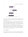
4.1
Collaboration diagram of class DCAcompressor . . . . . . . . . . . . . . .
30
4.2
Suffix trie generated by graphviz . . . . . . . . . . . . . . . . . . . . . . .
32
4.3
File compression/decompression . . . . . . . . . . . . . . . . . . . . . . . .
33
4.4
Implementation of static scheme . . . . . . . . . . . . . . . . . . . . . . .
34
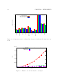
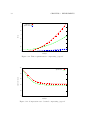
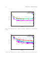
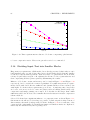
5.1
Memory requirements of different self-compression options . . . . . . . . .
48
5.2
Time requirements of different self-compression options
. . . . . . . . . .
48
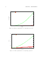
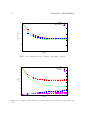
5.3
Compression ratio of different self-compression options . . . . . . . . . . .
49
5.4
Self-compression compression ratios on Canterbury Corpus . . . . . . . .
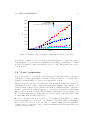
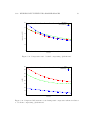
50
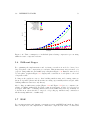
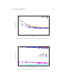
5.5
Number of nodes in relation to maxdepth
. . . . . . . . . . . . . . . . . .
50
5.6
Number of nodes leading to antiwords in relation to maxdepth . . . . . . .
51
xvii
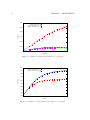
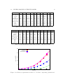
5.7
Number of antiwords in relation to maxdepth . . . . . . . . . . . . . . . .
52
5.8
Number of used antiwords in relation to maxdepth . . . . . . . . . . . . .
52
5.9
Relation between number of nodes and number of antiwords . . . . . . . .
53
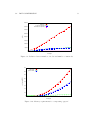
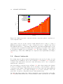
5.10 Memory requirements for compressing “paper1” . . . . . . . . . . . . . . .
53
5.11 Time requirements for compressing “paper1” . . . . . . . . . . . . . . . .
54
5.12 Compression ratio obtained compressing “paper1” . . . . . . . . . . . . .
54
5.13 Compressed file structure created using static scheme compressing “paper1” 55
5.14 Memory requirements for decompressing “paper1.dz” . . . . . . . . . . . .
56
5.15 Time requirements for decompressing “paper1.dz” . . . . . . . . . . . . .
56
5.16 Individual phases of compression process using suffix trie . . . . . . . . . .
57
5.17 Individual phases time contribution using suffix trie . . . . . . . . . . . .
58
5.18 Individual phases of compression process using suffix array . . . . . . . . .
58
5.19 Individual phases time contribution using suffix array . . . . . . . . . . .
59
5.20 Compression ratio obtained compressing “grammar.lsp” . . . . . . . . . .
60
5.21 Compression ratio obtained compressing “sum” . . . . . . . . . . . . . . .
60
5.22 Memory requirements using almost antiwords . . . . . . . . . . . . . . . .
61
5.23 Time requirements using almost antiwords . . . . . . . . . . . . . . . . . .
61
5.24 Compression ratio obtained compressing “paper1” . . . . . . . . . . . . .
62
5.25 Compressed file structure created using almost antiwords . . . . . . . . .
62
5.26 Compression ratio obtained compressing “alice29.txt” . . . . . . . . . . .
63
5.27 Compression ratio obtained compressing “ptt5” . . . . . . . . . . . . . . .
63
5.28 Compression ratio obtained compressing “xargs.1” . . . . . . . . . . . . .
64
5.29 Memory requirements in relation to block size compressing “plrabn12.txt”
65
5.30 Time requirements in relation to block size compressing “plrabn12.txt”
.
66
5.31 Compression ratio obtained compressing “plrabn12.txt” . . . . . . . . . .
67
5.32 Compressed file structure in relation to block size . . . . . . . . . . . . . .
67
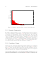
5.33 Dynamic compression scheme exception distances histogram . . . . . . . .
68
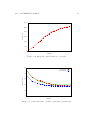
5.34 Exception count in relation to maxdepth . . . . . . . . . . . . . . . . . . .
69
5.35 Compression ratio obtained compressing “plrabn12.txt” . . . . . . . . . .
69
5.36 Best compression ratio obtained by each method on Canterbury Corpus .
70
xviii
5.37 Average compression ratio obtained on Canterbury Corpus . . . . . . . .
71
5.38 Average compression speed on Canterbury Corpus . . . . . . . . . . . . .
72
5.39 Average time needed to compress 1MB of input text . . . . . . . . . . . .
72
5.40 Memory needed to compress 1B of input text . . . . . . . . . . . . . . . .
73
5.41 Compression ratio obtained by selected methods on Canterbury Corpus .
73
5.42 Time needed to compress 1MB of input text . . . . . . . . . . . . . . . . .
74
5.43 Memory needed by selected methods to compress 1B of input text . . . .
74
xix
xx
List of Tables
2.1
Canterbury Corpus . . . . . . . . . . . . . . . . . . . . . . . . . . . . . . .
4
3.1
Suffix array for text “abcaab” . . . . . . . . . . . . . . . . . . . . . . . . .
19
3.2
Suffix array used for antidictionary construction . . . . . . . . . . . . . . .
20
3.3
Example of node gains as antiwords . . . . . . . . . . . . . . . . . . . . .
22
3.4
Dynamic compression example . . . . . . . . . . . . . . . . . . . . . . . .
26
4.1
DCAstate structure implementation . . . . . . . . . . . . . . . . . . . . .
35
4.2
Compressed file format . . . . . . . . . . . . . . . . . . . . . . . . . . . . .
40
5.1
Parallel antidictionaries using static compression scheme . . . . . . . . . .
65
5.2
Parallel antidictionaries using dynamic compression scheme . . . . . . . .
65
5.3
Best compression ratios obtained on Canterbury Corpus . . . . . . . . . .
70
5.4
Compressed file sizes obtained on Canterbury Corpus
. . . . . . . . . . .
75
5.5
Compressed file sizes obtained on Calgary Corpus . . . . . . . . . . . . . .
75
5.6
Pros and cons of different methods . . . . . . . . . . . . . . . . . . . . . .
75
xxi
xxii
Chapter 1
Introduction
1.1
Problem Statement
DCA (Data Compression using Antidictionaries) is a novel data compression method
presented by M. Crochemore in [6]. It uses current theories about finite automata and
suffix languages to show their abilities for data compression. The method takes advantage
of words that do not occur as factors in the text, i.e. that are forbidden. Thanks to
existence of these forbidden words, some symbols in the text can be predicted.
The general idea of the method is quite interesting, first input text is analyzed and all
forbidden words are found. Using binary alphabet Σ = {0, 1} symbols whose occurrences can be predicted using the set of forbidden words are erased. DCA is a lossless
compression method, which operates on binary streams.
1.2
State of The Art
Currently there are no available implementations of DCA, all were developed for experimental purposes only. Some research is being done on using larger alphabets rather than
binary and on using compacted suffix automata (CDAWGs) for antidictionary construction.
1.3
Contribution of the Thesis
In the thesis dynamic compression using DCA is explained and implemented and antidictionary construction using suffix array is introduced focusing on minimizing memory
requirements. Several methods based on data compression using antidictionaries idea are
implemented — static compression scheme as well as dynamic compression scheme and
static compression scheme with support for almost antifactors, that are words, which occur rarely in the input text. Their results compressing files from Canterbury and Calgary
1
2
corpus are presented.
1.4
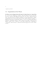
Organization of the Thesis
In Chapter 2 basic definitions and terminology used in the thesis can be found. Chapter 3 describes the way different methods of DCA are working, brings some examples and
also some new ideas. Furthermore dynamic compression scheme is described and antidictionary construction using suffix array is introduced. Also basics of different stages in
static compression scheme are explained. In Chapter 4 possible implementation of different DCA methods are presented along with some ideas of improving their performance or
limiting time and memory requirements. Chapter 5 focuses on experiments with different
parameters of implemented methods. Their comparison and results on Canterbury and
Calgary corpuses could be found here, provided with comments and recommendations
to their usage. The last chapter concludes the thesis and suggests some ideas for future
research.
Chapter 2
Preliminaries
Definition 2.1 (Lossless data compression)
A lossless data compression method is one where compressing a file and decompressing
it retrieves data back to its original form without any loss. The decompressed file and
the original are identical, lossless compression preserves data integrity.
Definition 2.2 (Lossy data compression)
A lossy data compression method is one where compressing a file and then decompressing
it retrieves a file that may well be different to the original, but is “close enough” to be
useful in some way.
Definition 2.3 (Symmetric compression)
Symmetric compression is a technique that takes about the same amount of time to
compress as it does to decompress.
Definition 2.4 (Asymmetric compression)
Asymmetric compression is a technique that takes different time to compress than it does
to decompress.
Note 2.1 (Asymmetric compression)
Typically asymmetric compression methods take more time to compress than to decompress. Some asymmetric compression methods take longer time to decompress, which
would be suited for backup files that are constantly being compressed and rarely decompressed. But basically faster compression than decompression is what we want for usual
compress once, decompress many times behaviour.
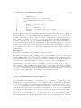
Note 2.2 (Canterbury Corpus)
The Canterbury Corpus[15] is a collection of “typical” files for use in the evaluation
of lossless compression methods. The Canterbury Corpus consists of 11 files, shown
in Table 2.1. Previously, compression software was tested using a small subset of one
or two “non-standard” files. This was a possible source of bias to experiments, as the
data used may have caused the programs to exhibit anomalous behaviour. Running
3
4
CHAPTER 2. PRELIMINARIES
File
alice29.txt
asyoulik.txt
cp.html
fields.c
grammar.lsp
kennedy.xls
lcet10.txt
plrabn12.txt
ptt5
sum
xargs.1
Category
English text
Shakespeare
HTML source
C source
LISP source
Excel spreadsheet
Technical writing
Poetry
CCITT test set
SPARC Executable
GNU manual page
Size
152089
125179
24603
11150
3721
1029744
426754
481861
513216
38240
4227
Table 2.1: Files in the Canterbury Corpus
compression software experiments using the same carefully selected set of files gives us a
good evaluation and comparison with other methods.
Note 2.3 (Calgary Corpus)
The Calgary Corpus[4] is the most referenced corpus in the data compression field especially for text compression and is the de facto standard for lossless compression evaluation.
It was founded in 1987. It is a predecessor of the Canterbury Corpus.
Definition 2.5 (Compression ratio)
Compression ratio is an indicator evaluating compression performance. It is defined as
Compression ratio =
Length of compressed data
.
Length of original data
Definition 2.6 (Alphabet)
An alphabet Σ is a finite non-empty set of symbols.
Definition 2.7 (Complement of symbol)
A complement of symbol a over Σ, where a ∈ Σ, is a set Σ \ {a} and is denoted ā.
Definition 2.8 (String)
A string over Σ is any sequence of symbols from Σ.
Definition 2.9 (Set of all strings)
The set of all strings over Σ is denoted Σ∗ .
Definition 2.10 (Substring)
String x is a substring (factor ) of string y, if y = uxv, where x, y, u, v ∈ Σ∗ .
5
Definition 2.11 (Prefix)
String x is a prefix of string y, if y = xv, where x, y, v ∈ Σ∗ .
Definition 2.12 (Suffix)
String x is a suffix of string y, if y = ux, where x, y, u ∈ Σ∗ .
Definition 2.13 (Proper prefix, factor, suffix)
A prefix, factor and suffix of a string u is said to be proper if it is not u.
Definition 2.14 (Length of string)
The length of string w is the number of symbols in string w ∈ Σ∗ and is denoted |w|.
Definition 2.15 (Empty string)
An empty string is a string of length 0 and is denoted ε.
Definition 2.16 (Deterministic finite automaton)
A deterministic finite automaton (DFA) is quintuple (Q, Σ, δ, q0 , F ), where Q is a finite
set of states, Σ is a finite input alphabet, δ is a mapping Q × Σ → Q, q0 ∈ Q is an initial
state, F ⊂ Q is the set of final states.
Definition 2.17 (Transducer finite state machine)
A transducer finite state machine is sixtuple (Q, Σ, Γ, δ, q0 , ω), where Q is a finite set
of states, Σ is a finite input alphabet, Γ is a finite output alphabet, δ is a mapping
Q × Σ → Q, q0 ∈ Q is an initial state, ω is an output function Q × (Σ ∪ {ε}) → Γ.
Definition 2.18 (Suffix trie [18])
Let T = t1 t2 · · · tn be a string over an alphabet Σ. String x is a substring of T . Each
string Ti = ti · · · tn where 1 ≤ i ≤ n + 1 is a suffix of T ; in particular, Tn+1 = ε is the
empty suffix. The set of all suffixes of T is denoted σ(T ). The suffix trie of T is a tree
representing σ(T ).
More formally, we denote the suffix trie of T as STrie(T ) = (Q ∪ {⊥}, Σ, root, F, g, f )
and define such a trie as an augmented deterministic finite-state automaton which has a
tree-shaped transition graph representing the trie for σ(T ) and which is augmented with
the so called suffix function f and auxiliary state ⊥. The set Q of the states of STrie(T )
can be put in a one-to-one correspondence with the substrings of T . We denote by x̂ the
state that corresponds to a substring x.
The initial state root node corresponds to the empty string ε, and the set F of the final
states corresponds to σ(T ). The transition function g is defined as g(x̂, a) = ŷ for all x̂, ŷ
in Q such that y = xa, where a ∈ Σ.
The suffix function f is defined for each state x̂ ∈ Q as follows. Let x̂ 6= root. Then
x = ay for some a ∈ Σ, and we set f (x̂) = ŷ. Moreover, f (root) = ⊥.
Automaton STrie(T ) is identical to the Aho-Corasick string matching automaton [1] for
the key-word set {Ti | 1 ≤ i ≤ n + 1} (suffix links are called in [1] failure transitions.)
6
CHAPTER 2. PRELIMINARIES
Definition 2.19 (Suffix trie depth)
Suffix trie depth k is the maximum height allowed for the trie. We will denote it as
maxdepth k.
Note 2.4 (Suffix trie depth limit)
Due to the suffix trie depth limit k, suffix trie represents only suffixes S ⊂ σ(T ), ∀x ∈ S :
|x| ≤ k.
Theorem 2.1 (Suffix trie [18])
Suffix trie ST rie(T ) can be constructed in time proportional to the size of ST rie(T )
which, in the worst case, is O(|T |2 ).
Definition 2.20 (Suffix tree [18])
Suffix tree STree(T ) of T is a data structure that represents STrie(T ) in space linear
in the length |T | of T . This is achieved by representing only a subset Q0 ∪ {⊥} of the
states of STrie(T ). We call the states in Q0 ∪ {⊥} the explicit states. Set Q0 consists of
all branching states (states from which there are at least two transitions) and all leaves
(states from which there are no transitions) of STrie(T ). By definition, root is included
into the branching states. The other states of STrie(T ) (the states other than root and ⊥
from which there is exactly one transition) are called implicit states as states of STree(T );
they are not explicitly present in STree(T ).
Note 2.5 (Suffix link)
Suffix link is a key feature for linear-time construction of the suffix tree. In a complete
suffix tree, all internal non-root nodes have a suffix link to another internal node. Suffix
link corresponds to function f (r) of state r. If the path from the root to a node spells
the string bv, where b ∈ Σ is a symbol and v is a string (possibly empty), it has a suffix
link to the internal node representing v.
Note 2.6 (Suffix tree)
Suffix tree represents all suffixes of a given string. It is designed for fast substring searching, each node represents a substring, which is determined by the path to the node. The
difference between suffix tree and suffix trie could be more obvious from Figure 2.1.
The large amount of information in each edge and node makes the suffix tree very expensive, consuming about ten to twenty times [11] the memory size of the source text in
good implementations. The suffix array reduces this requirement to a factor of four, and
researchers have continued to find smaller indexing structures.
Definition 2.21 (Antifactor [3])
Antifactor (or Forbidden Word ) is a word that never appears in a given text.
Let Σ be a finite alphabet and Σ∗ the set of finite words of symbols from Σ, the empty
word ε included.
Let L ⊂ Σ∗ be a factorial language, i.e. ∀u, v ∈ Σ∗ , uv ∈ L ⇒ u, v ∈ L. The complement
Σ∗ \ L of L is a (two sided) ideal of Σ∗ . Denote by MF(L) its base: Σ∗ \ L = Σ∗ MF(L)Σ∗ .
7
⊥
Σ
c
c o
a
c
a
o
a o
o
⊥
a
Σ
o
a
ca
cao
o
o
cao
o
Figure 2.1: Comparison of suffix trie (left) and suffix tree over string “cacao”
MF(L) is the set of Minimal Forbidden words for L. A word v ∈ Σ∗ is forbidden for L if
v∈
/ L. The forbidden word is minimal if it has no proper factors that are forbidden.
Definition 2.22
The set of all minimal forbidden words we call an antidictionary AD.
Definition 2.23 (Internal nodes)
The internal nodes of the suffix trie correspond to nodes actually represented in the trie,
that is, to factors of the text.
Definition 2.24 (External nodes)
The external nodes correspond to antifactors, and they are implicitly represented in
the tree by the null pointers that are children of internal nodes. The exception are
the (forcedly) external nodes at depth k + 1, that are children of internal nodes at the
maximum depth k, which may or may not be antifactors.
Definition 2.25 (Terminal nodes)
Each external node of the trie that surely corresponds to an antifactor (i.e. at depth < k)
is converted into an internal (leaf) node. These new internal nodes are called terminal
nodes.
Note 2.7 (Terminal nodes)
Note that not all leaves are terminal, as some leaves at depth k are not antifactors.
Definition 2.26 (Almost antifactor [7])
Let us assume that a given string s appears m times in the text, and that s.0 and s.1,
8
CHAPTER 2. PRELIMINARIES
where ‘.’ means concatenation1 , appear m0 and m1 times, respectively, so that m =
m0 + m1 (except if s is at the end of the text, where m = m0 + m1 + 1). Let us assume
that we need e bits to code an exception. Hence, if m > e ∗ m0 , then we improve the
compression by considering s.0 as an antifactor (similarly with s.1). Almost antifactors
are string factors, that improve compression when considered as antifactors.
Definition 2.27 (Suffix array)
Suffix array is a sorted list of all suffixes of given text represented by pointers.
Note 2.8 (Suffix array [12])
When a suffix array is coupled with information about the longest common prefixes (lcps)
of adjacent elements in the suffix array, string searches can be answered in O(P + log N )
time with a simple augmentation to a classic binary search, P is searched string length.
The suffix array and associated lcp information occupy a mere 2N integers, and searches
are shown to require at most P + dlog2 (N − 1)e single-symbol comparisons.
The main advantage of suffix arrays over suffix trees is that, in practice, they use three
to five times less space.
Definition 2.28 (Stopping pair [6])
A pair of words (v, v1 ) is called stopping pair if v = ua, v1 = u1 b ∈ AD, with a, b ∈
{0, 1}, a 6= b, and u is a suffix of u1 .
Lemma 2.1 (Only one stopping pair [6])
Let AD be an antifactorial antidictionary of a text t ∈ Σ∗ . If there exists a stopping pair
(v, v1 ) with v1 = u1 b, b ∈ {0, 1}, then u1 is a suffix of t and does not appear elsewhere in
t. Moreover there exists at most one pair of words having these properties.
1
The concatenation mark ‘.’ is omitted when it is obvious.
Chapter 3
Data Compression Using
Antidictionaries
3.1
DCA Fundamentals
DCA (Data Compression using Antidictionaries) is a novel data compression method
presented by M. Crochemore in [6]. It uses current theories about finite automata and
suffix languages to show their abilities for data compression. The method takes advantage
of words that do not occur as factors in the text, i.e. that are forbidden, we call them
forbidden words or antifactors. Thanks to existence of these forbidden words, we can
predict some symbols in the text.
Just imagine, that we have an antifactor w = ub, where w, u ∈ Σ∗ , b ∈ Σ and while
reading text, we find occurence of string u. Because the next symbol can’t be b, we can
predict it as b̄. Therefore when we compress the text, we erase symbols that can be
predicted and in reverse when decompressing we predict the erased symbols back.
The general idea of the method is quite interesting, first we analyze input text and find all
antifactors. Using binary alphabet Σ = {0, 1} we erase symbols, whose occurrences can
be predicted using the set of antifactors. As we can see, DCA is a lossless compression
method, which operates on binary streams so far, i.e. it is working with single bits, not
symbols of larger alphabets, but some current research is dealing with this, too.
Example 3.1
Compress string s = u.1, s ∈ Σ∗ , using antifactor u.0.
Because u.0 is an antifactor, the next symbol after u must be 1. So we can erase the
symbol 1 after u.
To be able to compress the text, we need to know the forbidden words. First we analyze
the input text and find all antifactors, which can be used for text compression (Figure 3.1).
For our purpose, we don’t need all antifactors, but just the minimal ones. The antifactor
9
10
CHAPTER 3. DATA COMPRESSION USING ANTIDICTIONARIES
Figure 3.1: DCA compression basic scheme
is minimal when it does not have any proper factor, that is forbidden. The set of all
minimal antifactors — the antidictionary AD is sufficient, because for every antifactor
w = uv, where u is a string over Σ, there exists a minimal antifactor v in antidictionary
AD.
Currently there is not any known good working implementation of the DCA compression
method. Yet we are trying to develop it, we are still far from practical use, due to the
excessive system resources needed to compress even a small file. However thanks to rapid
research progress of strings, suffix arrays, suffix automata (DAWGs), compacted suffix
automata (CDAWGs) and other related issues, we might be able to design a practical
implementation soon.
3.2
Data Compression and Decompression
Let w be a text on the binary alphabet {0, 1} and let AD be an antidictionary for w
[6]. By reading the text w from left to right, if at a certain moment the current prefix
v of the text admits as suffix a word u0 such that u = u0 x ∈ AD with x ∈ {0, 1}, i.e. u
is forbidden, then surely the symbol following v in the text cannot be x and, since the
alphabet is binary, it is the symbol y = x̄. In other terms, we know in advance the next
symbol y, that turns out to be redundant or predictable.
The main idea of this method is to eliminate redundant symbols in order to achieve
compression. The decoding algorithm recovers the text w by predicting the symbol
following the current prefix v of w already decompressed.
Example 3.2
Compress text 01110101 using antidictionary AD = {00, 0110, 1011, 1111}:
step:
input:
1
0
|
output: 0
2
01
|.
0
3
011
|./
01
4
0111
|./.
01
5
01110
|./..
01
6
011101
|./...
01
7
0111010
|./....
01
8
01110101
|./.....
01
1. Current prefix: ε. There is no such word x in AD, so we pull 0 from input and push
11
3.2. DATA COMPRESSION AND DECOMPRESSION
it to output.
2. Current prefix: 0. There is word 00 in AD, so we erase the next symbol (1).
3. Current prefix: 01. There is no such word u = u0 x in AD, where u is suffix of 01.
We read 1 from input and push it to output.
4. Current prefix: 011. There is word 0110 in AD, so we erase the next symbol (1).
5. Current prefix: 0111. There is word 1111 in AD, so we erase the next symbol (0).
..
.
The result of compressing text 01110101 is 01. To be able to decompress this text, we
need to store the antidictionary and the original text length also, which could be more
obvious from the following decompression example.
Example 3.3
Decompress text 01 using antidictionary AD = {00, 0110, 1011, 1111}.
Decompression is just an inversed compression algorithm:
1. Current prefix: ε. There is no such word x in AD, so we pull 0 from input and push
it to output.
2. Current prefix: 0. There is word 00 in AD, so we predict the next symbol as 1 and
push it to output.
3. Current prefix: 01. There is no such word u = u0 x in AD, where u is suffix of 01.
We read 1 from input and push it to output.
4. Current prefix: 011. There is word 0110 in AD, so we predict the next symbol as 1
and push it to output.
5. Current prefix: 0111. There is word 1111 in AD, so we predict the next symbol 0
and push it to output.
..
.
step:
input:
1
0
|
output: 0
2
0
|
01
3
01
| \
011
4
01
| \
0111
5
01
| \
01110
6
01
| \
011101
7
01
| \
0111010
8
01
| \
01110101
After decompression of text 01 we get the original text 01110101. What is important is
that we don’t know exactly when to stop the algorithm by knowing just the compressed
text and the antidictionary. This means we need to know the length of the original text or
we could decompress even infinitely. Another possibility is to store the number of erased
12
CHAPTER 3. DATA COMPRESSION USING ANTIDICTIONARIES
⊥
Σ
⊥
⊥
Σ
⊥
c
Σ
a
⊥
c
Σ
c
a
a
c
a
a
c
c
c
c
Σ
a
a o
c o
a
a
c
c
o
a
a
a
o
o
Figure 3.2: Constructing suffix trie for text “cacao”
symbols after using the last input bit, which could be sufficient for most implementations,
but this supposes that we can determine exactly end of the input text.
For compression and decompression process, the antidictionary must be able to answer
the query on a word v, if there exists a word u = u0 x, x ∈ {0, 1}, u ∈ AD such, that u0
is a suffix of v. The answer determines, if the symbol x will be kept or erased in the
compressed text. To speedup the queries, we can represent the antidictionary as a finite
transducer, which leads to fast linear-time compression and decompression. Then we can
compare it to the fastest compression methods. To build the compression/decompression
transducer, we need a special compiler, that builds the antidictionary first, and then
constructs the automaton over it.
3.3
Antidictionary Construction Using Suffix Trie
As it turns out later, the most complex task of the DCA method is just the antidictionary
construction. It’s natural to use suffix trie structure for collecting all factors of the given
text, although any other data structure for storing factors of words can be used, such
as suffix trees, suffix automata (DAWGs), compacted suffix automata (CDAWGs), suffix
arrays, . . .
Let’s consider text t = c1 c2 c3 . . . cn of length n, where ci is a symbol at position i. We
are adding words c1 , c1 c2 , c1 c2 c3 , . . . , c1 c2 c3 . . . cn step by step. Because we are adding
the words to a suffix trie structure representing all suffixes of the given words, we get all
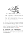
factors of text t. See Figure 3.2 for example of constructing suffix trie for text “cacao”.
To construct an antidictionary from the suffix trie, we add all antifactors of the text. For
every factor u = u0 x, we add an antifactor v = u0 y, x 6= y, if factor v doesn’t already
exist. The resulting antidictionary won’t be minimal so we need to select only the minimal
antifactors. The antifactor v is minimal when there does not already exist an antifactor
13
3.3. ANTIDICTIONARY CONSTRUCTION USING SUFFIX TRIE
0
00
1
010
0
0101
0
0
ε
1
0
1
01
1
011
0111
0
01110
ε
0
1
0
10
101 0
1010
1
10101
10
0
110
1
1101
111
0
1110 1
0
1
0111
0
0
1
11010
01110
01111
100
101 0
1
1
11
0
1
0110
1010
1
0
1011
1
11
011
0
1
1
1
1
1
01
1
0101
0
0
1
010
0
1
0100
1
11011
1110 1
0
1
11101
1111
11100
110
111
0
11101
10100
1
0
0
1
1100
10101
1101
11010
00
0
00
0
0
ε
010
011
0
1
0
1
01
1
0
0100
1
0101
0110
0111
0
1
0
1
1
0
10
0
1
11
01111
100
101 0
1
1
0
1
01110
1
1010
0
10101
1011
10100
1
0
11011
1110 1
0
1
11101
1111
11100
110
0
1
111
0
1100
1101
11010
ε
0110
0
0
1
01
1
0
10
1
011
0
1
1
101
1
1011
1
11
1
111
1
1111
Figure 3.3: Antidictionary construction over text “01110101” using suffix trie
w such that v = v 0 w, i.e. there is no such antifactor w, that is a suffix of v. This can
be easily checked using suffix link (dashed line in Figure 3.2). The antifactor v = u0 y
is minimal, when f (u0 )y is an internal node, otherwise a shorter antifactor w certainly
exists.
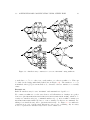
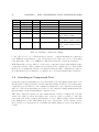
Example 3.4
Build an antidictionary for text “01110101” with maximal trie depth k = 5.
We construct a suffix trie over the text, then we add all antifactors. Antifactors together
form a set {00, 100, 0100, 0110, 1011, 1100, 1111, 01111, 11100, 11011, 10100}, which is obviously not antidictionary (set of minimal antifactors), e.g. 00 is a suffix of antifactors
100, 0100, 1100, 11100, 10100. We have to remove antifactors, that are not minimal. Resulting set is antidictionary AD = {00, 0110, 1011, 1111}. See Figure 3.3 for suffix trie
construction process. On the final diagram we can see trie containing only necessary
nodes to represent the antidictionary, leaf nodes are antifactors.
14
CHAPTER 3. DATA COMPRESSION USING ANTIDICTIONARIES
00
0
0
ε
0110
0
1
01
1
011
0
0
1
1
0
10
1
101
ε
1
1011
1
1/ε
0/0
01
1/1
011
0/0
1/1
1
0/0
10
1/ε
101
0/ε
11
1/1
0/0
1
111
1/ε
0/ε
11
1
1111
1/1
111
Figure 3.4: Antidictionary AD = {00, 0110, 1011, 1111} and the corresponding compression/decompression transducer
For representing the antidictionary we don’t need the whole tree, so we keep only the
nodes and links, which lead to antifactors. This simplified suffix trie is going to be used
later for compression/decompression transducer building.
3.4
Compression/Decompression Transducer
As we have suffix trie of the antidictionary now, which is in fact an automaton accepting
antifactors, we are able to construct a compression/decompression transducer from it.
From every node r except terminal nodes we have to make sure that transitions for
both 0/1 symbols are defined. For a missing transition δ(r, x), x ∈ {0, 1}, we create this
transition as δ(f (r), x). As we do this in breadth-first search order, δ(f (r), x) is always
defined. The only exception is the root node, which needs special handling. Transducer
construction can be found in more detail in [6] as “L-automaton”.
Then we remove the terminal states and assign output symbols to the edges. The output
sybols are computed as follows: if a state has two outgoing edges, output symbol is the
same as the input one; if a state has only one outgoing edge, output symbol is an empty
word (ε). An example is presented in Figure 3.4.
3.5. STATIC COMPRESSION SCHEME
15
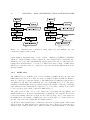
Figure 3.5: Basic antidictionary construction
3.5
Static Compression Scheme
Antidictionary is needed to build the compression/decompression transducer, but in practical applications the antidictionary is not apriori given, we need to derive it from the
input text or from some “similar data source”. We build the antidictionary using one
of the techniques mentioned in Section 3.3. With bigger antidictionary we could obtain
better compression, but it grows with the length of input text and we need to control its
size, or its representation will be inefficient and the compression could be very slow. A
rough solution is to limit length of the words belonging into antidictionary, which is done
by limiting suffix trie depth during its construction. This will simplify and lower the system requirements for building the antidictionary. This simple antidictionary construction
scheme is presented in Figure 3.5.
3.5.1
Simple pruning
In static compression scheme we compress and decompress the data with the same antidictionary. However the decompression process has to know the original antidictionary,
that was used for compression. That’s why we need to store the used antidictionary
together with the compressed data. The question is, if the stored antiword will erase
more bits, than the bits needed to actually store the antiword. Possible antidictionary
representations will be discussed in Section 4.5.
Let’s consider that we know, how many bits are needed for representation of each antiword, then we can compute the gain of each antiword and prune all antiwords with
negative gain. We call this simple pruning. After applying this function on the antidictionary, we can improve the compression ratio of the static compression scheme by storing
only the “good” antiwords and using just them for compression. Our static compression
scheme will now look like Figure 3.6.
16
CHAPTER 3. DATA COMPRESSION USING ANTIDICTIONARIES
Figure 3.6: Antidictionary construction using simple pruning
3.5.2
Antidictionary self-compression
As with static approach we need to store the antidictionary together with the compressed data, it might cross our minds, that there is a possibility to compress also the
antidictionary itself. This depends heavily in which form we are going to represent the
antidictionary list. Basically we have two options:
1. antiword list – antidictionary size, length of each antiword and the antiword itself.
With this we could use all previous antiwords to compress/decompress the following
antiwords, e.g. for AD = {00, 0110, 1011, 1110} we get AD0 = {00, 010, 101, 1110}.
2. antiword trie – trie structure represented in some suitable way. Using this method
we are actually saving a binary tree, of course the tree can be also self-compressed.
Longer antiwords can be compressed using shorter antiwords, but with some limitations.
Let’s consider the following, w = ubv is an antiword, u, v ∈ Σ∗ , b ∈ Σ. If we
compressed antiword w = ubv using antiword z = ub̄, it would become w0 = uv and
|w0 | = |z| could happen, which means, that nodes representing antiwords z and w0
would be on the same level in the compressed suffix trie and could overlap. This is
generally not what we want, because we wouldn’t be able to reconstruct the original
tree. Reasonable solution is to erase symbol b from antiword w = ubv if and only
if there exists antiword y = xb̄, where x is a proper suffix of u, which makes sure,
that |w0 | > |y|.
Example 3.5
Self-compress trie of the antidictionary AD = {00, 0110, 1011, 1110}:
Only 1011 antiword path can be compressed, we remove node 101 as it can be predicted
due to antiword 00 and connect nodes 10 and 1011. Antiword 1011 will actually become
3.6. ANTIDICTIONARY CONSTRUCTION USING SUFFIX ARRAY
17
00
0
ε
0110
0
0
1
01
1
0
10
1
011
0
1
1
101
1
1011
(101)
1
1
11
1
111
1
1111
Figure 3.7: Self-compression example
101 in the new representation. Antiword 0110 cannot be compressed, because compressing
01 to just 0 will lead to a nondeterministic antidictionary reconstruction. See Figure 3.7.
Self-compression algorithm will be explained thoroughly in Section 4.4.4.
With antidictionary self-compression we can further improve our static compression
scheme. And what about combining this technique with simple pruning? In fact it
makes things a bit harder, because self-compressing changes the antidictionary representation and influences antiword gains. For better precision we do simple pruning on a
self-compressed tree and after pruning we self-compress the antidictionary and consider
it as final.
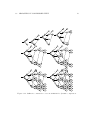
However this simplification isn’t accurate, after self-compressing the trie still may not be
optimal, because on the other side simple pruning affects self-compression. We can fix
this by applying simple pruning and self-compressing iteratively as long as some nodes
are pruned from the trie. Both single and multiple self-compression/simple prune rounds
are demonstrated in Figure 3.8.
3.6
Antidictionary Construction Using Suffix Array
In previous sections we used suffix trie for antidictionary construction. One of the main
problems of suffix trie structure is its memory consumption, the large amount of information in each edge and node make it very expensive. Even for depth k larger than 30 and
small input files, suffix trie size grows very fast and needs tens to hundreds Megabytes of
memory. Also creation and traversal through the whole trie is quite slow.
We can consider other methods for collecting all text factors. As we are dealing with
18
CHAPTER 3. DATA COMPRESSION USING ANTIDICTIONARIES
(a)
(b)
Figure 3.8: Antidictionary construction using single (a) and multiple (b) selfcompression/simple prune rounds
binary alphabet, this limits usage of some of them — suffix trees, DAWGs or CDAWGs,
which are designed mainly for larger alphabets. Also antidictionary constructing algorithms need to be modified fundamentally and an appropriate way for efficiently representing these structures has to be developed. This work focuses on usage of suffix arrays,
which were a favourite subject to study in recent years and many implementations are
already available.
3.6.1
Suffix array
The suffix trees were originally developed for searching for suffixes in the text. Later the
suffix arrays were discovered. They are used for example in Burrows-Wheeler Transformation [5] and bzip2 compression method. The suffix array is a sufficient replacement for
the suffix trees allowing some tasks that were done with suffix trees before. The major
advantage is much smaller memory requirements and also smaller complexity considering
some tasks performed during DCA compression, e.g. node visits counting. It is possible
to save even more space using compressed suffix arrays [9].
The suffix array is built on top of the input text, representing all text suffixes and
alphabetically sorted. In fact it contains indexes pointing into the original text. Because
for most algorithms, this is not enough, we also build lcp array on top of the input text
and suffix array. An example of suffix array can be seen in Table 3.1. Symbol # denotes
the end of the text, lexicographically the smallest symbol.
Lcp (Least Common Prefix) array contains the adjacent word prefix length common with
the previous word. With just these two structures we can do all needed operations, as we
will show later. String searches can be answered with a complexity similar to the binary
3.6. ANTIDICTIONARY CONSTRUCTION USING SUFFIX ARRAY
i
ti
SA
LCP
0
a
6
0
#
1
b
3
0
a
a
b
#
2
c
4
1
a
b
#
3
a
0
2
a
b
c
a
a
b
#
4
a
5
0
b
#
5
b
1
1
b
c
a
a
b
#
19
6
#
2
0
c
a
a
b
#
Table 3.1: Suffix array for text “abcaab”
search, a memory representation requires two arrays of pointers, one for suffix array and
one for lcps, their sizes are equivalent to the length of input text.
Let’s suppose we have an efficient algorithm for suffix array and lcp construction. What
we need to realize for antidictionary construction is, that we are constructing suffix array
over the binary alphabet, so the suffix array and lcp length will be 8 times length of
the input text. Still memory requirements for suffix array construction depends only on
the length of input text with O(N ), instead of suffix trie almost exponential complexity,
depending on the trie depth.
3.6.2
Antidictionary construction
The suffix arrays offer text searching capabilities similar to suffix tries, thus why not
to use them for antidictionary construction. First mention of this idea can be found
in [19]. Now antidictionary construction using suffix array with asymptotic complexity
O(k ∗ N log N ) will be explained, k is maximal antiword length. The process takes two
adjacent strings at a time and finds antifactors. Special handling is needed for the last
item, which is not in pair.
1. Take two adjacent strings ui and ui+1 from suffix array, ui , ui+1 ∈ Σ∗ .
2. Skip their common prefix c utilizing LCP, ui = cxv, ui+1 = cyw, x 6= y and test the
first differing symbol, c, v, w ∈ Σ∗ , x, y ∈ Σ. If x = #, y = 1, then add antifactor
c.0.
3. For each symbol vj of string ui = cxv such, that vj = 0, add antifactor
cxv1 . . . vj−1 1.
4. For each symbol wj of string ui+1 = cyw such, that vj = 1, add antifactor
cyw1 . . . wj−1 0.
5. Repeat previous steps for all suffix array items.
20
CHAPTER 3. DATA COMPRESSION USING ANTIDICTIONARIES
i
ti
SA
LCP
0
0
8
0
#
1
1
6
0
0
1
#
2
1
4
2
0
1
0
1
#
3
1
0
2
0
1
1
1
0
4
0
7
0
1
#
5
1
5
1
1
0
1
#
6
0
3
3
1
0
1
0
1
7
1
2
1
1
1
0
1
0
8
#
1
2
1
1
1
0
1
Table 3.2: Suffix array for binary text “01110101” highlighting antifactor positions
6. For the last item un = v, for each symbol vj = 0, add antifactor v1 . . . vj−1 1.
This simple algorithm finds all text antifactors, we only need to limit antifactor length.
Using this technique we find all antifactors, but what we really want are minimal antifactors. One possible way is to construct a suffix trie from the found antifactors and
then choose just the minimal antifactors using suffix links. Second option is to utilize the
suffix array ability for searching strings.
To check if antifactor u = av, a ∈ {0, 1} is minimal, try to find string v in the suffix array.
If string v appears in the text, then the antifactor u is minimal. Search for a string in
suffix array equipped with lcp array takes O(P + log N ) time, where P is length of v.
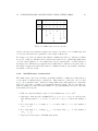
Example 3.6
Build antidictionary for text “01110101” using suffix array.
First we build suffix array and lcp structure, it can be seen in the Table 3.2, suffix tree for
the same text can be found in Figure 3.3. Using algorithm introduced above we find possible antifactors, their positions are marked with a frame around symbols. Positions with
minimal antifactors are underlined. This leads to the set of minimal antifactors, antidictionary AD = {00, 0110, 1011, 1111}, which corresponds with antidictionary computed
using suffix trie.
3.7
Almost Antifactors
The idea of almost antifactors was introduced in [7]. After more detailed examination
of antidictionaries we can discover also their odd behaviour. If we try to compress the
string 10n−1 with k ≥ 2, then the result is satisfying because we can use {01, 11} as our
antidictionary. This permits compressing the string to (1, n) plus the small antidictionary.
However, if we reverse the string to 0n−1 1, then for any k < n the set of antifactors
contains {10, 11}, which indeed does not yield any compression. The classical algorithm
produces an empty antidictionary. Yet, both strings have the same 0-order entropy.
3.7. ALMOST ANTIFACTORS
21
As we can see, the main problem is that a single occurrence of a string in the text (in
our second example the string “01”) outrules it as an antifactor. In a less extreme case,
it may be possible that a string sb, s ∈ Σ∗ , b ∈ Σ appears just a few times in the text,
but its prefix s appears so many times, that it is better to consider sb as an antifactor.
Of course, to be able to recover the original text, we need to code somehow those text
positions where the bit predicted by taking the string as an antifactor is wrong. We
call exceptions the positions in the original text where this happens, that is, the final
positions of the occurrences of sb in the text.
3.7.1
Compression ratio improvement
Usage of almost antifactors can theoretically bring compression ratio improvement to
original DCA algorithm, but it’s not so easy, as it looks at the first sight. By introducing
some almost antifactors we can remove also “good” antifactors, whose gain was better
than of the newly introduced almost antiword. Also we completely prune branches connected to factors we turned into antifactors. In contrast of improving gain, introducing
new almost antiwords we lose some gain elsewhere, the whole tree changes a lot.
The key problem [7] is that the decision of what is an almost antifactor depends in turn on
the gains produced, so we cannot separate the process of creating the almost antifactors
and computing their gains: creating an almost antifactor changes the gains upwards in
the tree, as well as the gains downwards via suffix links. So there seems to be no suitable
traversal order. It is not possible either to do a first pass computing gains and then a
second pass deciding which will be terminals, because if one converts a node into terminal
its gain changes and modifies those of all the ancestors in the tree. It is not possible to
leave the removal of redundant terminals for later because the removal can also change
previous decisions on ancestors of the removed node.
3.7.2
Choosing nodes to convert
In the original document two ways of solving this problem were introduced, one-pass and
multi-pass heuristics. Both heuristics work with the whole suffix trie, not with just the
trie with antifactors. This is very limiting for designing a fast DCA implementation,
multi-pass heuristics needs repetitious tree traversal over the whole suffix trie, which is
very expensive.
Although we can use the one-pass heuristics, according to [7] it doesn’t perform as well
as the multi-pass one. The one-pass heuristics first makes breadth-first top-down traversal determining which nodes will be terminal, and then applies the normal bottom-up
optimization algorithm to compute gains and decide which nodes deserve belonging to
the antidictionary.
The problem of heuristics is that it’s not accurate, since considering that it may be a
bad decision to convert into terminal a node that turns out to have a subtree with a
large gain, we lose it, an also when we give the preference to the highest node, it is not
necessarily always the best choice. Even when testing one-pass heuristics with deeper
22
CHAPTER 3. DATA COMPRESSION USING ANTIDICTIONARIES
[15]
0
[16]
ε
0
1
0
[14]
00
0
01 [1]
1
1
1
000 [13]
001 [1]
[1]
Figure 3.9: Example of using almost antiwords
Node
0
1
00
01
000
001
Gain as an antiword
16 − 5 ∗ 15 = 59
16 − 5 ∗ 1 = 11
15 − 5 ∗ 14 = −55
15 − 5 ∗ 1 = 10
14 − 5 ∗ 13 = −51
14 − 5 ∗ 1 = 9
Table 3.3: Example of node gains as antiwords
suffix tries, we can get worse results than with the classical approach, it depends on the
particular file. Using multi-pass heuristics, k/2 passes count are recommended for good
results, but it is not suitable for us because of its time complexity.
Example 3.7
Compress text 0000000000000001 = 015 1 using suffix trie depth limit k = 3 with classical
approach and with almost antiwords, then compare the results.
We build suffix trie from the text, as can be seen in Figure 3.9. Next to each node
there is a visit count written in brackets. Let’s suppose the following: representation of
every node in antidictionary trie takes A = 2 bits + 2 extra bits for coding root node,
representation of each exception takes E = 5 bits. Now we can compute gain of each
node r as an antiword using function g(r), p(r) is parent of r, v(r) is visit count of r,
g(r) = v(p(r)) − E ∗ v(r).
After gain computation (see Table 3.3) we convert node 1 to a terminal node because of
its positive gain. Nodes 01 and 001 are not converted, because they would be not minimal
antifactors. We obtain antidictionary AD = {1}, which compresses the input data to ε.
Using classical approach we get an empty dictionary, which means no compression at all.
Our output will look like
lenclassical = empty AD(2b) + original length(5b) + data(16b) = 23b.
Using almost antiword approach we get the antidictionary with one word, one exception
3.8. DYNAMIC COMPRESSION SCHEME
23
Figure 3.10: Dynamic compression scheme
and empty compressed data, our output size will be
lenalmost-aw = AD(2b + 2b) + original length(5b) + data(0b) + exception(1 ∗ 5b) = 14b.
As we can see, using almost antiword improvement we saved 9 bits in comparison with
classical approach and this could be even more interesting for longer texts.
3.8
Dynamic Compression Scheme
Till now we were considering static compression model, where the whole text must be
read twice, once when the antidictionary is computed and once when we are actually
compressing the input. Using this method we need to store the antidictionary separately.
To do it in an efficient way, we use techniques like simple pruning and self-compression.
But there is also another possible solution how to use DCA algorithm. With dynamic
approach we read text only once, we compress input and modify antidictionary at the
same time. Whenever we read some input, we recompute the antidictionary again and
use it for compressing the next input (Figure 3.10). The compression process can be
described in these steps:
1. Begin with an empty antidictionary.
2. Read input and compress it using the current antidictionary.
3. Add the read symbol to the factor list and recompute antidictionary.
24
CHAPTER 3. DATA COMPRESSION USING ANTIDICTIONARIES
4. Every exception that occurs, code and save into separate file.
5. Repeat steps until the whole input processed.
Because we don’t know the correct antidictionary in advance, we are making mistakes in
predicting the text. Every time we read a symbol that violates the current antidictionary
and brings a forbidden word, we need to handle this exception. We do it by saving
distances between the two adjacent exceptions. This can be represented by number of
successful compressions (bits erased) between the exceptions, there is no need to count
symbols just passed to the algorithm in non-determined transitions. Exception occurs
only when there exists a transition with ε output from the current state, but we don’t
take it.
Exceptions can be represented by some kind of universal codes, arithmetic or Huffman
coding. It needs to be stored along the compressed data in a separate file or when we use
output buffers large enough, they can be a direct part of compressed data.
3.8.1
Using suffix trie online construction
For compressing text using the dynamic compression model we don’t need a pruned
antidictionary or even a set of minimal antifactors, because the compressor and the
decompressor share both the same suffix trie, they can use all available antifactors directly.
With advantage we can use suffix tries for representing already collected factors as well
as for compressing the input online. We use the suffix trie as an automaton, maintaining
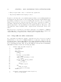
suffix links. For this we can use the following algorithm:
1
2
3
4
5
6
7
8
9
10
11
12
13
14
15
16
17
18
19
20
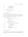
1
2
Dynamic−Build−Fact (int maxdepth > 0)
root ← new state;
level(root) ← 0;
cur ← root;
while not EOF do
read(a);
p ← cur;
if level(p) = maxdepth then
p ← fail(p);
while p has no child and p 6= root do
p ← fail(p);
if p has only one child δ(p, x) then
if x = a then
erase symbol a
else
write exception;
else
write a to output;
cur ← Next(cur,a,maxdepth);
return root;
Next (state \textit{cur}, bool a, int maxdepth > 0)
if δ(cur, a) defined then
3.8. DYNAMIC COMPRESSION SCHEME
3
4
5
6
7
8
9
10
11
12
25
return δ(cur, a)
else if level(\textit{cur}) = maxdepth then
return Next(fail(\textit{cur}), a, maxdepth)
else
q ← new state;
level(q) ← level(\textit{cur}) + 1;
δ(cur, a) ← q;
if cur = root then fail(q) = root;
else fail(q) ← Next(fail(\textit{cur}),a,maxdepth);
return q;
Function Dynamic-Build-Fact() builds suffix trie and compresses data at once, function
Next() takes care of creating suffix links and missing nodes up to the root node. For
dynamic compression we need to know only δ(p, a) transitions, fail function and current
level of the node, where p is some node, a ∈ {0, 1}. This is less than half information
needed for each node and edge in comparison with suffix trie representation in static approach, which means less memory requirements. Considering time asymptotic complexity
of Dynamic-Build-Fact() gives us only O(N ∗ k), which is identical to suffix trie construction complexity in Section 4.4.1, but already compressing text where static compression
scheme starts.
Example 3.8
Compress text 11010111 using dynamic compression scheme.
We start compressing from the beginning, but it could be useful to skip some symbols and
get the suffix trie filled a bit. It’s typical to get many exceptions at the beginning, because
the suffix trie is only forming at first. This is subject for further experiments. Suffix trie
construction process with antifactors found in every step can be seen in Figure 3.11.
Compression process in steps can be seen in Figure 3.4. We get output: “0 E 1 . E . E .”,
where C means compressed, E means exception and ‘.’ is an empty space after erased symbol. Totally 3 exceptions, 3 compressions occurred and 2 symbols were passed. What
we can see, is that antidictionary changes only when we pass a new symbol or when an
exception occurs, while the set of all antifactors can change any time.
3.8.2
Comparison with static approach
We can think about advantages of this method: we don’t have to separately code the
antidictionary, do self-compression or even to simple prune it. We simply use all antifactors found yet. Memory requirements are smaller, method is quite fast, as it does not
need to do breadth first search for building antidictionary or any other tree traversal for
computing gains. Even it is very simple to implement it if we don’t bother with suffix
trie memory greediness and we don’t need to read the text twice as in the static scheme.
There are some disadvantages, too, decompression will be slower, it makes the method
symmetric, because decompression process must do almost the same as compression. As
we build antidictionary dynamically, parallel compressors/decompressors are not possible
26
CHAPTER 3. DATA COMPRESSION USING ANTIDICTIONARIES
input
0
1
1
1
0
1
read text
1
01 (E)
011
0111 (C)
01110 (E)
011101 (C)
output
0
except
1
0
0111010 (E)
except
1
01110101 (C)
except
antidictionary
1
00
00, 10
00, 10
00, 010, 0110, 1111
00, 010, 0110, 1111
00, 0110, 1011, 1111
00, 0110, 1011, 1111
all antifactors
1
00
00, 10, 010
00, 10, 010, 110, 0110
00, 010, 0110, 1111, 01111
00, 010, 100, 0110, 1100,
1111, 01111, 11100
00, 100, 0110, 1011, 1100,
1111, 01111, 11011, 11100
00, 100, 0110, 1011, 1100,
1111, 01111, 10100, 11011,
11100
Table 3.4: Dynamic compression example
to use, also we lose one of DCA strong properties — pattern matching in compressed
text. Efficient representation of the exceptions is a problem, but can be solved using
some universal coding or e.g. Huffman coding and storing the exceptions separately.
With this method, it is possible to reach better compression ratios than with the static
compression scheme. These results were presented in the original paper [6]. But as this
method is not asymmetric and the decompression has the same complexity as compression, this method is not suitable for compress once, decompress many times behaviour.
3.9
Searching in Compressed Text
Compressed pattern matching is a very interesting topic and many studies have been
already made on this problem for several compression methods. They focus on linear time
complexity proportional not to the original text length but to the compressed text length.
And one of the most interesting properties of text compressed using antidictionaries is
just its ability of pattern matching in compressed text.
This data compression method doesn’t transform the text in a complex way, but just
erases some symbols. From the single point of view it could be possible to erase just
some symbols from the searched pattern and look for it. This is really possible, but with
some limitations, because what symbols we erase depends also on the current context.
If we search for a long pattern, we can utilize its synchronizing property, from which we
obtain:
27
3.9. SEARCHING IN COMPRESSED TEXT
00
00
0
0
00
ε
0
0
0
0
ε
ε
1
1
01
1
0
10
011
0
1
10
0
0111
0
0
01110
01111
ε
1
01
0
1
011
0111
0110
0111
0
1
1
0
10
0
1
01110
01111
100
101
1
0
1
110
0
1
11
0
1
1110
110
0
1
111
0
1
1111
0
00
0
010
0
01
1
011
00
0
1
0
0110
0111
0
1
0
1
0
0110
010
0
1
1
111
1
110
0
10
11
ε
0
1
0
1
111
1
0
011
1
0110
1
1
1
1
00
0
0
01
11
1
1
ε
010
1
1
11
0
1
0
0
1
1
0
011
0
0
1
1
00
ε
01
01
1
0
0
1
0
1
010
0
1
010
0
10
0
1
01111
100
101 0
1
11
0
1
11011
1110 1
0
1
11101
1111
11100
0
1
111
0
1100
1101
1
11010
11101
1111
11100
011
0
1
0101
0110
0111
0
1
0
0
10
0
1
101 0
1
1010
1
0
1011
11
0
1
01110
01111
100
1
1
0
110
ε
01
1
1110 1
0
1
1
1010
1011
1
0
01110
1
1101
0100
010
0
1100
10100
1
0
11011
1110 1
0
1
11101
1111
11100
110
0
1
111
0
1100
10101
1101
11010
Figure 3.11: Suffix trie construction over text 01110101 for dynamic compression
28
CHAPTER 3. DATA COMPRESSION USING ANTIDICTIONARIES
Lemma 3.1 (Synchronizing property [17])
If |w| ≥ k − 1, then δ ∗ (u, w) = δ ∗ (root, w) for any state u ∈ Q such that δ ∗ (u, w) ∈
/
AD, where w is the searched pattern, k is length of the longest forbidden word in the
antidictionary, Q is the set of all compression/decompression transducer states, function
δ ∗ (u, w) is the state reached after applying all transitions δ(ui , bi ), i = 1 . . . i|w| , u1 =
u, ui = δ(ui−1 , bi−1 ), w = b1 b2 . . . b|w| , b ∈ {0, 1}.
Unfortunately this works only for patterns longer than k, so we need to search the compressed text using a different technique presented in [17], which solves the problem in
O(m2 + kM k + n + r) time using O(m2 + kM k + n) space, where m and n are the pattern length and the compressed text length respectively, kM k denotes the total length of
strings in antidictionary M , and r is the number of pattern occurrences.
This is achieved using a decompression transducer with eliminated ε-states similar to the
one mentioned in [8] and an automaton build over the search pattern. The algorithm
has a linear complexity proportional to the compressed text length, when we exclude the
pattern processing. This pattern searching algorithm can be used on texts compressed
using static compression method, because it needs to preprocess the antidictionary before
searching starts, not on texts produced by dynamic method, which also lacks synchronization property of static compressed texts.
Chapter 4
Implementation
4.1
Used Platform
The main target of this thesis was to implement a working DCA implementation, try
different parameters of the method and choose the most appropriate. Program was
intended to work on command line and be as efficient as possible. Many tests were
needed to run as a batch, the program was to be licensed under some public licence,
and that’s why GNU/Linux platform for selected for development. Also small memory
requirements, low CPU usage and other optimization factors were demanded.
As C/C++ is a native language for development on most platforms, C++ language using
gcc compiler (g++ respectively), which also suits best for its built-in optimizations, was
preferred. Using C++ we have memory management of dynamically allocated memory in
our hands, we don’t need to rely on a garbage collector. The program was developed for
32 bit platforms, it would need further modifications to work under 64 bit environment.
For good portability GNU tools Automake and Autoconf were used, that automatically
generate build scripts for target platform. The program was tested only under i586
platform, which uses little endian, for big endian platforms modifications would be needed.
Nevertheless this program serves still rather for research and testing purposes, it is not
usable as a production tool, despite the efforts it is not practically usable because of its
high system resources requirements. As the code is published under GNU/GPL, everyone
can use the code, experiment with it and try to improve it.
4.2
Documentation and Versioning
Because program code was changing a lot during development, a versioning system Subversion, which remembers all the changes, can find differences to the current version or
provide a working version from the past, was used. This ability was used more than
once, as to get the algorithm working correctly is quite difficult. Huge data structures
are built in the memory, suffix tries are modified online, traversed in different ways and
29
30
CHAPTER 4. IMPLEMENTATION
snext
next
epsilon
asc
fail
dca::D CAstate
original
stPoolLim it
trie
stPool
dca::D CAstateC
next
asc
com pTrie
dca::D CAantidict
ad
dca::D CAcom pressor
Figure 4.1: Collaboration diagram of class DCAcompressor
directions and it is a challenge to debug what is really going on. Although we can verify
compressed data by decompressing them, this doesn’t tell us anything about optimal
selection of forbidden words or correct and complete building of the data structure for
representing all text factors.
Documentation was written along with the code using documentation generator Doxygen.
This documentation generator takes the program source code, extracts all classes, functions and variables definitions and provides them with comments specified in the source,
output formats are HTML and LATEX. Unlike offline documentation systems Doxygen
keeps the documentation up-to-date. An example of collaboration diagram of class DCA
created by Doxygen in cooperation with Graphviz can be seen on Figure 4.1.
We can’t rely just on this type of documentation, as it does not describe, how the algorithms work in common, only describes the meaning of each variable and how the
functions are called. For that type of documentation some Wiki system, LATEX or another kind of offline documentation is more appropriate. It should also support including
tables and graphics for better descriptions of used data structures and algorithms. At
this point this text is serving for this purpose.
4.3
Debugging
As was mentioned before, it was needed to debug, how the program was really performing
some tasks, including building trie and its online modification. Normal program debuggers as gdb are not very useful, as we need to see the program outputs and contents of
4.3. DEBUGGING
31
large data structures contained in memory. Therefore the program was equipped with
different debugging options to provide information about each part of the process, they
can be turned on in compile time by defining the following macros:
• DEBUG – if not set, turns off all debugging messages, otherwise shows debugging
messages according to LOG_MASK filter; also enables counters of total nodes and
nodes deleted during simple pruning,
• DEBUG_DCA – enables trie and antidictionary debugging, every node contains also
its complete string representation, which enlarges memory requirements a lot,
• PROFILING – turns on/off profiling info designated for performance measurements.
Profiling is using POSIX getrusage() function and reads ru_utime and ru_stime representing user time and system time used by the current process. These times are measured
at the beginning and at the end of the measured program part, if the procedure runs
more times, the measured time is accumulated. For this purpose classes TimeDiff_t and
AccTime_t are provided, the first measures time interval, the second measures accumulated time. What we need to know, is that using getrusage() function also influences the
program performance, especially the accumulated time measurement of a program part
repeated many times. With --verbose option the program reports the whole time taken
to perform the operation as well as antidictionary size and compression ratio achieved.
CPU time consumption is just one part of system requirements, what we are very interested in, too, is a memory consumption. It was measured using memusage utility that
comes from the GNU libc development tools and it is a part of many GNU/Linux distributions. This tool reports the peak memory usage of heap and stack extra. What
we are interested in more is the heap peak size, as the most memory used is allocated
dynamically. Also the amount of allocated and correctly deallocated memory could be
seen. But in fact we don’t really need to check it as the program compresses only one file
at a time and the memory is automatically deallocated when the program terminates.
For debugging purposes LOG_MASK was introduced to have the ability to select what we
really want to debug and not to be choked up with other extensive useless debug messages.
LOG_MASK is a set of the following items:
• DBG_MAIN – print information about which part of the algorithm is currently being
run,
• DBG_TRIE – debug suffix trie data structures and displays its contents in different
parts of algorithm; it also exports the contents into graphviz graph file language for
drawing directed graphs using dot tool,
• DBG_COMP – debug compression process, shows read symbols, used transitions in
compression transducer, compressed symbols,
• DBG_DECOMP – debug decompression process, shows read symbols, used transitions
and symbol output,
32
CHAPTER 4. IMPLEMENTATION
0
01010
0101
1
1
00
01011
010
0
0
0
0
1
01
1
011
0110
1
0
0111
10101
1
e
1
1
0
10
1
0
1010
101
1
1
1011
11
0
110
1
1
1
0
1101
10111
11010
1
111
11011
Figure 4.2: Suffix trie for text “11010111” generated by graphviz
• DBG_PRUNE – debug simple pruning process, gain computation, traversal over the
suffix trie, tested and pruned nodes,
• DBG_AD – prints antidictionary and self-compressed antidictionary contents in different stages of algorithm, such as before and after simple pruning,
• DBG_STATS – print some useful statistics, like results of simple pruning, antidictionary self-compression and overall algorithm performance,
• DBG_ALMOSTAW – debug almost antifactors related information,
• DBG_PROFILE – show profiling info.
One of the most useful options is the antidictionary debugging, which stores antidictionary
state in different stages to an external file for later examination. From this we can find out
if the antidictionary construction is working properly or which antiwords are problematic.
With this we have an essential hint for finding implementation errors.
Another important option is the trie debugging, which outputs a trie structure in a text
format as well as in a graphical format created using graphviz1 . It is possible to even watch
the suffix trie construction step by step. Regardless these graphs are drawn automatically
and are not so nice as diagrams drawn by hand, they can be still very handy. An example
of a suffix trie graph generated by graphviz can be seen on Figure 4.2.
4.4
Implementation of Static Compression Scheme
In Section 3.5 has been already outlined how the antidictionary and compression transducer is prepared for static compression scheme. Let’s look at overview what we actually
1
Graph Visualization Software — open source graph (network) visualization project from AT&T Research, http://www.graphviz.org/
4.4. IMPLEMENTATION OF STATIC COMPRESSION SCHEME
(a)
33
(b)
Figure 4.3: File compression (a) and file decompression (b) schemes
do with a ready-made transducer. In Figure 4.3 both compression and decompression
process schemes can be found, examining both processes further.
With static compression scheme after building the antidictionary and compression transducer we have already read the whole text, we know its length and we can easily compute
its CRC32 checksum while building the antidictionary. As the decompression process
needs to know the length of original data, we save this, along with CRC32 for verifying
data integrity, into the output file. Then we save the antidictionary using one of the
methods discussed in Section 4.5. And only after this we start compressing the input
data using the compression transducer and writing its product to the output file.
The decompression process should be clear. First we read the data length, CRC32 and
we load the antidictionary into the memory in a suffix trie representation. Then we selfdecompress the trie updating all suffix links and creating decompression transducer at a
time. With prepared transducer we run decompression until we get originalLen amount
of data, writing the product to output file and calculating CRC32 of decompressed data.
At the end we verify the checksum and notify user of decompression result (CRC OK or
description of which error occurred).
In Section 3.5 antidictionary construction process has been presented, but it was not
complete. Actually “Build Automaton” phase must be executed one more time just after
“Build Antidictionary” stage to fix all incorrect suffix links and forward edges pointing to
removed nodes, as they are required for self-compression. After this correction, antidictionary construction with single self compression and single simple pruning round looks
like this: Figure 4.4. Now individual stages will be described in more detail.
4.4.1
Suffix trie construction
For suffix trie construction an algorithm very similar to the one presented in [6] is used.
Function Build-Fact() reads input and builds suffix trie adding new nodes, fvis(r) is
direct visits count of node r. Function Next() takes care of creating all suffix links and
34
CHAPTER 4. IMPLEMENTATION
Figure 4.4: Real implementation of static scheme antidictionary construction with selfcompression and single simple pruning
missing nodes up to the root node. b(r) is the input symbol leading to node r, visited (r)
is total visits of the node, used later for gain computation, asc(r) is parent of node r,
fail (r) is suffix link of node r. antiword (r) and deleted (r) indicate node status, awpath(r)
indicates, if there exists a path from root node to some antiword through node r. Time
asymptotic complexity of Build-Fact() is O(N ∗ k).
1
2
3
4
5
6
7
8
9
10
Build−Fact (int maxdepth > 0)
root ← new state;
level(root) ← 0; fvis(root) ← 0; visited(root) ← 0;
deleted(root) ← false; antiword(root) ← false; awpath(root) ← false;
cur ← root;
while not EOF do
read(a);
cur ← Next(cur, a, maxdepth);
fvis(cur) ← fvis(cur) + 1;
return root;
1
2
3
4
5
6
7
8
9
10
11
12
13
Next (state cur, bool a, int maxdepth > 0)
if δ(cur, a) defined then
return δ(cur, a)
else if level(cur) = maxdepth then
return Next(fail(cur), a, maxdepth)
else
q ← new state;
level(q) ← level(cur) + 1; fvis(q) ← 0; visited(q) ← 0; b(q) ← a;
deleted(q) ← false; antiword(q) ← false; awpath(q) ← false;
δ(cur, a) ← q;
if cur = root then fail(q) = root;
else fail(q) ← Next(fail(cur), a, maxdepth);
return q;
4.4. IMPLEMENTATION OF STATIC COMPRESSION SCHEME
struct DCAstate
DCAstate* next[0..1]
DCAstate* snext[0..1]
DCAstate* fail
DCAstate* asc
DCAstate* epsilon
int visited, fvis, level
bool b, awpath, antiword
(a)
35
struct DCAstateC
DCAstateC* next[0..1]
DCAstateC* asc
DCAstate* original
int gain
bool b
(b)
Table 4.1: DCAstate structure (a) representing a suffix trie node and DCAstateC structure (b) representing a node in self-compressed trie
Suffix trie nodes are represented by DCAstate structure (Figure 4.1a), next represents δ
transitions, snext represents δ 0 , epsilon represents ε transitions, other variables represent
functions with corresponding names. For representation of nodes in self-compressed trie
there is used another structure — DCAstateC (Figure 4.1b), which is more efficient,
meaning of variables is similar to DCAstate variables, original is a pointer to an original
node in non-compressed trie.
4.4.2
Building antidictionary
Function Build-AD() walks through the tree and adds all minimal antifactors. Using
function MarkPath() it marks all nodes in the path from root node to the antiword.
Then using traversal in depth-first order it computes node total visits and removes all
nodes, that does not lead to any antiword. We also omit stopping pair antifactors as they
don’t bring any compression. Time asymptotic complexity of Build-AD() is O(N ∗ k 2 ),
which makes it strongly dependant on maxdepth k.
1
2
3
4
5
6
7
8
9
10
11
12
13
14
15
16
17
18
Build−AD (root)
for each node p, level(p) < k in breadth−first order do
for a ∈ {0, 1} do
if δ(p, a) defined then
δ 0 (p, a) = δ(p, a)
else if δ(fail(p), a) defined and δ(p, ā) defined then
q ← new state;
δ 0 (p, a) ← q;
antiword(q) ← true;
MarkPath(q);
for each node p, not antiword(p) in depth−first order do
if fvis(p) > 0 then
vis ← 0;
q ← p;
while q 6= root
if fvis(q) > 0 then
vis ← vis + fvis(q);
fvis(q) ← 0;
36
CHAPTER 4. IMPLEMENTATION
19
20
21
22
23
24
1
2
3
4
4.4.3
q ← fail(q);
visited(q) ← visited(q) + vis;
if not awpath(p) then
if asc(p) defined then
δ 0 (asc(p), b(p)) ← NULL;
deleted(p) ← true;
MarkPath(p)
while p defined and not awpath(p) do
awpath(p) ← true;
p ← asc(p);
Building automaton
After building antidictionary and removing all nodes not leading to antiwords, the trie
is not consistent, some of the suffix links are pointing to deleted nodes. This has to be
fixed before self-compressing the trie. At the same time we correct the suffix links, we
also define new δ transitions and ε transitions creating a compression transducer. Time
asymptotic complexity of Build-Automaton is O(N ∗ k).
1
2
3
4
5
6
7
8
9
10
11
12
13
14
15
16
17
18
19
20
21
4.4.4
Build−Automaton (root)
for a ∈ {0, 1} do
if δ 0 (root, a) defined and not deleted(δ 0 (root, a)) then
δ(root, a) ← δ 0 (root, a);
fail(δ(root, a)) ← root;
else
δ(root, a) ← root;
if antiword(δ(root, a)) for a ∈ {0, 1} then
ε(root) ← δ(root, ā);
for each node p, p 6= trie in breadth−first order do
for a ∈ {0, 1} do
if δ 0 (p, a) defined and not deleted(δ 0 (p, a)) then
δ(p, a) ← δ 0 (p, a);
fail(δ(p, a)) ← δ(fail(p), a);
else if not antiword(p)
δ(p, a) ← δ(fail(p), a);
else
δ(p, a) ← p;
if not antiword(p) then
if antiword(δ(p, a)) for a ∈ {0, 1} then
ε(p) ← δ(p, ā);
Self-compression
Using self-compression we create a new compressed trie from the original trie and initialize
gain values g0 (r) of all nodes to −1. This is necessary for the simple-pruning algorithm, as
it walks the trie bottom-up and needs to know, if both subtrees were already processed.
4.4. IMPLEMENTATION OF STATIC COMPRESSION SCHEME
37
The original (r) value is a pointer to the original code in non-compressed suffix trie. Time
asymptotic complexity is O(N ∗ k).
1
2
3
4
5
6
7
8
9
10
11
12
13
14
15
16
17
18
19
4.4.5
Self−Compress (root)
rootCompr ← new state;
add (root, rootCompr) to empty queue Q;
while Q 6= ∅ do
extract (p,p0 ) from Q;
if q0 and q1 are children of p then
create q00 and q10 as children of p0 ;
original(q00 ) ← q0 ; original(q10 ) ← q1 ;
g0 (q00 ) ← −1; g0 (q10 ) ← −1;
add (q0 , q00 ) and (q1 , q10 ) to Q;
else if q is a unique child of p, q = δ(p, a), a ∈ {0, 1} then
if antiword(δ(p, ā)) then
add (q, p0 ) to Q;
else
create q 0 as a−child of p0 ;
original(q 0 ) ← q;
g0 (q 0 ) ← −1;
add (q, q 0 ) to Q;
return rootCompr;
Gain computation
Gain computation is based on the fact, that we can estimate gain of a node being an
antifactor, if we know how much costs its representation. For this 2 + 2 representation
is used for antidictionary storage, described in Section 4.5. Gain g 0 (S) of subtree S is
defined as in [6]:


0


 c(S) − 2
if
if
g 0 (S) =
0
 g (S1 ) − 2 if



M
if
S
S
S
S
is empty,
is a leaf (antiword),
has one child S1 ,
has two children S1 and S2 ,
where M = max(g 0 (S1 ), g 0 (S2 ), g 0 (S1 ) + g 0 (S2 )) − 2. It is clear, that it is possible to
compute gains in linear time with respect to the size of the trie in a single bottom-up
traversal of the trie. But how the self-compression affects our gain computation? The
answer is, that it doesn’t in fact, we simply compute the gains using the self-compressed
tree!
4.4.6
Simple cruning
Simple pruning function prunes from the trie all nodes which does not have positive
gain. Gain function is computed using the self-compressed trie. As we are walking
the trie bottom-up from terminal nodes, the traversal is not deterministic and it’s not
38
CHAPTER 4. IMPLEMENTATION
guaranteed, that in each node we process, gains of both subtrees are already computed.
For this we have set g 0 (r) of each node r to value −1, which means uninitialized value,
if we hit a node with an uninitialized subtree, we stop walking bottom-up and continue
with the next antiword. After processing all antiwords, all trie nodes will have a defined
gain.
Whenever we find a node with negative gain, we prune it with the whole subtree belonging
to it and at the same time we prune also the subtree from the orginal trie. As we forbid
nodes with negative gains, we can simplify function M = max(g 0 (S1 ), g 0 (S2 ), g 0 (S1 ) +
g 0 (S2 )) − 2 from Section 4.4.5 to M 0 = g 0 (S1 ) + g 0 (S2 ).
Because this is not the only one possibility of static compression scheme implementation, for testing purposes simple-pruning was implemented also without self-compression.
Because it is very similar to the version using self-compression, only the more interesting version of simple pruning the self-compressed trie is going to be presented. Using
O(N ) for antidictionary size according to [14] and O(2k ) for pruning subtree we get time
asymptotic complexity O(N ∗ k ∗ 2k ).
1
2
3
4
5
6
7
8
9
10
11
12
13
14
15
16
17
4.5
Simple−Prune (rootCompr)
for each node p, antiword(p) do
while p 6= rootCompr do
q ← asc(p);
if antiword(original(p)) then
g0 (p) ← visited(asc(original(p))) − 2
else if p has children p1 , p2 then
if g0 (p1 ) = −1 or g0 (p2 ) = −1 then
break;
g0 (p) ← g0 (p1 ) + g0 (p2 ) − 2
else if p has child pp then
if g0 (pp) = −1 then
break;
g0 (p) ← g0 (pp) − 2;
if g0 (p) <= 0 then
prune subtree p; prune subtree original(p);
p ← q;
Antidictionary Representation
In static compression scheme we need to provide the compressed data with the andictionary used for compression in order to be able to decompress it. And as the antidictionary size reaches about 50% of the compressed data length, we know antidictionary
is really important and has a great significance to the final compression ratio. As in the
original paper 2+2 representation is used, but other possibilities are also discussed.
• antiword list – probably the least efficient storage for antiwords, it is not using
any common prefixes, but has better abilities for self-compression, as mentioned in
Section 3.5.2.
4.5. ANTIDICTIONARY REPRESENTATION
39
• 2+2 – binary tree with k nodes is encoded using 2k bits for the whole tree. Using
depth-first order we encode in each node, if it has both subtrees, only the right
subtree, only the left subtree or no subtree, by the strings 00, 01, 10, 11.
• 3+1 – representation introduced in [7], we traverse the tree in depth-first order and
write a 1 bit each time we find an internal node and a 0 bit each time we find an
external node. Therefore, a binary tree of m internal nodes will need exactly 2m+1
bits, which is almost identical to the 2+2 scheme.
• Hamming coding – first we walk the trie in depth-first order and count the times
we go left, right and up. Then we compute Hamming coding for these directions
and encode the trie by a depth-first walk. After experiments with this coding, we
found, that it is better only on very unbalanced trees, in other cases it performs
worse then 2+2.
• Text Generating the Antidictionary – an interesting idea, of how to code an antidictionary, is to supply some short text, that generates the target antidictionary.
This representation could be very efficient, this option is going to be discussed more
thoroughly.
In this DCA implementation 2+2 representation was used with the following meaning:
code
00
01
10
11
4.5.1
meaning
no subtree
only the right subtree
only the left subtree
both subtrees
Text generating the antidictionary
While playing with antidictionaries and their automata a new possibility of representing
antidictionaries was thought up. It seems to be feasible to code the antidictionary even
more efficiently. Such antidictionary would be generated from a special text and then
this antidictionary would be used for text decompression. The idea is based on fact,
that for an antidictionary AD 6= ∅ generated from string Tx , whose automaton contains
cycles, there exists some string Ty , which generates the same antidictionary AD, Tx 6= Ty ,
|Ty | ≤ |Tx |.
To be more efficient than representation R, we need to find a text Ty generating antidictionary AD, |Ty | < rsize(R, AD), where rsize is number of bits used by representation R
to code antidictionary AD. Problem is that this method probably won’t work for general
pruned antidictionaries. An in-depth future research on this topic is needed. Another
problem is, that the generating text Ty should contain the original stopping pair. Different text ending could lead to new unwanted antiwords. An example of antidictionary
whose compression/decompression transducer contains a loop is provided.
40
CHAPTER 4. IMPLEMENTATION
size
3B
item
“DCA”
4B
original length
4B
CRC32
*
*
antidictionary
compressed data
description
text identificator to unambiguously identify DCA compressed file
length of the original input text, this length is important
when decompressing data to determine end of the decompression process
cyclic redundancy check of the original data, it is computed
and checked during decompression
antidictionary representation as specified in Section 4.5
data with bits erased using DCA compression
Table 4.2: Compressed file format
Example 4.1
Let’s suppose that we have an antidictionary AD built over string “01010101”, AD =
{00, 11}. If we encodeded it using 2+2 representation, we would get antidictionary size
|AD| = 2 ∗ k = 10 bits, as the trie has k = 5 nodes. It is easy to see, that the text “010”
generates the same antidictionary, while it needs only 3 bits for coding the generating
text and a few bits for coding the text length.
Two promising ways of generating text Ty were found. The first uses compression transducer processing input text Tx avoiding loops, that don’t bring new nodes into suffix
trie. The second walks back from the stopping pair using transitions and suffix links
in inversed directions until it walks through all nodes. Both methods may not work on
general suffix tries, rather on the non-pruned constructed from a real text string, but this
needs more experiments.
Disadvantage of this representation is slower decompression, because we need to build
the antidictionary first from text Ty , also the decompressor must use the same method
as compressor to reconstruct the antidictionary. Another problem could be complexity
of constructing text Ty in compression process. Still antidictionary representation using
a generating text looks promising.
4.6
Compressed File Format
To be able to store the files compressed using DCA, a compressed file format had to be
developed. The proposed file format is similar to the one used by gzip and contains only
the necessary fields, targeting it to representing files compressed by static compression
scheme. CRC32 is used to check integrity of the decompressed data. See Table 4.2.
4.7. ANTIDICTIONARY CONSTRUCTION USING SUFFIX ARRAY
4.7
4.7.1
41
Antidictionary Construction Using Suffix Array
Suffix array construction
In these days we have a choice between many algorithms for suffix array construction.
They were a subject to test in [16], according which the used implementation were chosen.
Problem is that these algorithms are designated to 8 bit symbols, while we need just 0’s
and 1’s for antidictionary construction. It was obvious that it was necessary to make
some modifications to the existing implementation to handle binary alphabet.
According to the paper [16], none of the new linear time construction algorithm would
be a good choice for their large constants and memory requirements, instead a highly
optimized Manzini-Ferragina implementation [13] with non-linear asymptotic complexity
in almost all the tests performed better in both memory consumption and CPU time used.
Their implementation using C was modified to compile under C++ and also adjusted the
algorithm to use just 1 bit symbols, instead of 8 bits in input text. Corrections were
applied to deep sort, shallow sort and bucket sort subroutines. LCP algorithm did not
need this adjustment. But because the whole algorithm wasn’t examined well, after this
8 bit to 1 bit modification, the whole algorithm could be not optimal now. This would
need a further study and may be some more optimal algorithm for computing suffix array
of a bit array could be developed.
The whole byte is now used for representation of just a single bit, that means the algorithm
is now wasting 7 bits for each single bit of input text. Addressing single bits in bytes was
not tested, but it is very likely that addressing a single bit and swapping bits would need
more CPU time, while memory occupied by the whole input text expanded 8 times is still
marginal in comparison with the total memory needed for representing the compression
transducer.
4.7.2
Antidictionary construction
Anyway we have a working suffix array construction algorithm and we are going to use
it for antidictionary construction. An outline of antidictionary construction using the
suffix array was already presented in Section 3.6. In this implementation functions BuildAD-SA(), SA-Bin-Search() and Add-Antiword () are used, where the first one is the most
important doing most of the job finding all possible antifactors, SA-Bin-Search() checks
if the antifactor is minimal and Add-Antiword () adds the new antiword to the suffix trie
and computes visit counts of the added nodes. Symbol ’#’ denotes end of string, function
substr (str, ind, len) returns substring of string str starting at position ind of length len,
functions makeSA() and makeLCP () return suffix array and LCP array for specified text.
Time asymptotic complexity of Build-AD-SA is O(k ∗ N (log N + k)), which is similar
to complexity of building antidictionary from suffix trie, but with memory requirements
O(N ) thanks to suffix array representation. This assumpts, that we are able to count
number of node visits in O(k), which can be done during walking through the suffix+lcp
array. In this implementation it is O(N ) in worst case, but in average it is much smaller,
42
CHAPTER 4. IMPLEMENTATION
this implies total asymptotic complexity O(k ∗ N (N + log N )).
1
2
3
4
5
6
7
8
9
10
11
12
13
14
15
16
17
18
19
20
21
22
23
24
25
26
27
28
29
30
31
32
33
34
35
36
37
38
39
40
41
1
2
3
4
5
6
7
8
9
Build−AD−SA (root, int crc, int maxdepth > 0)
read whole input → bittext;
crc ← computeCRC32(bittext);
expand each single bit in bittext to 1 byte;
sa ← makeSA(bittext); lcp ← makeLCP(bittext, sa);
root ← new state; level(root) ← 0; fail(root) ← root;
for i ← 0 to |sa| do
lo ← 1; hi ← |sa|; l ← lcp[i + 1];
if l = maxdepth then
continue;
wcur ← substr(bittext, sa[i], maxdepth);
wnext ← substr(bittext, sa[i + 1], maxdepth);
if wcur [l] = ’#’ then {end of current word}
if wnext [l] = ’1’ then {’#’→’1’}
aw ← substr(wnext , 0, l) . ’0’;
if SA−Bin−Search(bittext, sa, aw, lo, hi) then
Add−Antiword(root, lcp, aw, i + 1);
else if wnext [l] = ’#’ then {end of next word}
if wcur [l] = ’0’ then {’0’→’#’}
aw ← substr(wcur , 0, l) . ’1’;
if SA−Bin−Search(bittext, sa, aw, lo, hi) then
Add−Antiword(root, lcp, aw, i);
lo2 ← lo; hi2 ← hi;
for ll ← l + 1 to |wcur | − 1 do
if (wcur [ll] = ’0’) then
aw ← substr(wcur , 0, ll) . ’1’;
if SA−Bin−Search(bittext, sa, aw, lo, hi) then
Add−Antiword(root, lcp, aw, i);
for ll ← l + 1 to |wnext | − 1 do
if wnext [ll] = ’1’ then
aw ← substr(wnext , 0, ll) . ’0’;
if SA−Bin−Search(bittext, sa, aw, lo2, hi2) then
Add−Antiword(root, lcp, aw, i + 1);
if |sa| > 0 then {process the last word}
lo ← 1; hi ← |sa|;
wcur ← substr(bittext, sa[|sa| − 1], maxdepth);
for l ← 0 to |wcur | − 1 do
if wcur [l] = ’0’ then
aw ← substr(wcur , 0, l) . ’1’;
if SA−Bin−Search(bittext, sa, aw, lo, hi) then
Add−Antiword(root, lcp, aw, |sa| − 1);
SA−Bin−Search (bittext, sa, aw, lo, hi)
pos ← 0;
tofind ← substr(aw, 1, |aw| − 1);
while hi ≥ lo do {at first find |tofind| − 1 characters}
pos ← (hi + lo)/2;
if sa[pos] + |tofind| − 1 < |sa| then
str ← substr(bittext, sa[pos], |tofind| − 1);
if str = substr(tofind, 0, |str|) then
break;
4.7. ANTIDICTIONARY CONSTRUCTION USING SUFFIX ARRAY
10
11
12
13
14
15
16
17
18
19
20
21
22
23
24
25
26
27
28
29
30
31
32
33
34
35
36
37
38
39
40
41
1
2
3
4
5
6
7
8
9
10
11
12
13
14
15
16
17
else if str < substr(tofind, 0, |str|) then
hi ← pos − 1;
else
lo ← pos + 1;
else
str ← substr(bittext, sa[pos], |sa| − sa[pos]);
if str < substr(tofind, 0, |str|) then
hi ← pos − 1;
else
lo ← pos + 1;
if hi < lo then
return false;
lo2 ← lo; hi2 ← hi;
while hi2 ≥ lo2 do {find exact string}
pos ← (hi2 + lo2)/2;
if sa[pos] + |tofind| < |sa| then
str ← substr(bittext, sa[pos], |tofind|);
if str = substr(tofind, 0, |str|) then
break;
else if str < substr(tofind, 0, |str|) then
hi2 ← pos − 1;
else
lo2 ← pos + 1;
else
str ← substr(bittext, sa[pos], |sa| − sa[pos]);
if str < substr(tofind, 0, |str|) then
hi2 ← pos − 1;
else
lo2 ← pos + 1;
if hi2 < lo2 then
return false;
return true;
Add−Antiword (root, lcp, aw, saPos)
p ← root;
for i ← 0 to |aw| − 1 do
if δ 0 (p, aw[i]) not defined then
q ← new state; asc(q) ← p; level(q) ← i + 1;
δ 0 (p, aw[i]) ← q;
p ← q;
else
p ← δ 0 (p, aw[i]);
antiword(p) ← true;
j ← saPos; k ← saPos;
len ← |aw| − 1;
while lcp[j] ≥ len do
j ← j − 1;
while k < n and lcp[k + 1] ≥ len do
k ← k + 1;
visited(asc(p)) ← k − j + 1;
43
44
4.8
CHAPTER 4. IMPLEMENTATION
Run Length Encoding
As discussed before, classical DCA approach has a problem with compressing strings of
type 0n 1, although it compresses well string 1n 0. We can improve these simple repetitions
handling by including RLE compression before the input of the DCA algorithm. Run
length encoding is a very simple form of lossless data compression in which runs of data,
i.e. sequences of the symbol, are stored as a single data value and count, rather than as
the original run. We compress all sequences with length ≥ 3 with count encoded using
Fibonacci code [2]. Sequences shorter than 3 are kept untouched.
Example 4.2
Compress text “abbaaabbbbbbbbbbbbbbba” = ab2 a3 b15 a using RLE.
In the input text there are two sequences with length ≥ 3, a3 and b15 . We compress the
first as “aaa0”, zero means no other “a” symbols. We compress the second sequence in a
similar way, resulting in “bbb12”. Our compressed text will be “abbaaa0bbb12a”.
4.9
Almost Antiwords
In order to improve the compression ratio also the almost antiwords improvement discussed in Section 3.7 was tested implementing the one-pass heuristics. It is based on
the suffix trie implementation, but an algorithm for building antidictionary with almost
antiwords support could be probably also developed.
The results were little disappointing at the beginning, later showed up that the modified
algorithm performs very good on some types of texts, while being worse than classical
approach on others. Another significant issue is, that the gain of almost antiwords is based
on an unknown factor of exception length, which can be only roughly estimated. Fine
tuning this implementation would probably lead to better results. For coding exceptions
Fibonacci code [2] was used again.
4.10
Parallel Antidictionaries
Unlike classical dictionary compression algorithms working with symbols, DCA is working
with a binary stream, where each considered symbol can gain only values ‘0’ and ‘1’. This
is very limiting, because we lose notion of symbol boundaries in text, as most English text
documents use only 7 bit symbols and we could just forget about the 7th bit, as it remains
‘0’. What was subject to test, was to slice a file lengthwise creating 8 files “fileN” with 0th
bit in “file0”, 1st bit in “file1” and so on, and then compressing these portions separately
using different antidictionaries. Using these approach 8 parallel antidictionaries over a
single file were simulated.
4.11. USED OPTIMIZATIONS
4.11
45
Used Optimizations
To optimize the code, some well-known optimizations as pointer arithmetics when working
with arrays, loop unrolling, dynamic allocation in large pools of prepared data were used.
Dynamic allocation has a significant impact on the performance, that’s why more memory
than needed is allocated at a time. Compiler optimizations were used, too, it is even
possible to use profiler log to gain better performance.
4.12
Verifying Results
During development many compression problems occurred. For verifying results extensive
logging was used and also some tools for checking the algorithm performance had to be
written, such as antidictionary generation, self-compression results and gain computation.
The best verification we have is, that after decompression we get the original text, however
this tells us nothing about the optimality of the used antidictionary. It has to be checked
some other way.
After antidictionary construction using suffix array was implemented, there has been an
advantage of two completely different methods for generating the antidictinary. Comparing outputs of these two different algorithms gives us a very good hint, if the generated
antidictionary is correct. So to verify the complete antidictionary is quite easy, but verification of the simple pruning process is impossible in fact, as there is no algorithm for
constructing the most efficient antidictionary available.
It’s much easier with self-compression. Self-compression check was implemented using a
dummy python script, which compresses all antiwords using all shorter ones. Performance
is quite slow, but the result is sufficient.
Also after code rewriting or implementing something new the new code has to be tested
every time on a set of files if it compresses and decompresses them correctly. This all was
possible thanks to strong scripting abilities of the GNU/Linux environment and without
all the verification tools it would not be so easy.
4.13
Dividing Input Text into Smaller Blocks
Earlier the memory greediness of DCA method and some options of reducing these requirements were discussed. Still one of the simplest options is to divide the file into
smaller blocks and compress them separately. This will reduce memory requirements
a lot, as the trie memory size depends strongly on the length of input text. On the
other hand we need to realize that this will affect compression ratio, which will be worse,
because the antidictionary will be smaller and the gains of antifactors will be lower.
46
CHAPTER 4. IMPLEMENTATION
Chapter 5
Experiments
5.1
Measurements
All measurements were executed on an AMD Athlon XP 2500+, 1024MB RAM, with
Mandriva Linux and kernel version 2.6.17 i686. All time measurements were made 5
times, for time measurements the minimal achieved value was selected, for memory measurements only one measurement was sufficient, as the algorithm is deterministic and use
the same amount of memory every time for the same configuration. Memory was measured using memusage from GNU libc development tools summarizing heap and stack
peak usage. Time was measured using getrusage() as a sum of user and system time
used. Program was compiled with “-O3” and DEBUG, PROFILING, MEASURING options turned on and all debug logging turned off. Program was called with “-v” option
displaying summary with compressed data length, antidictionary size, compression ratio
achieved and total time taken.
We are going to choose appropriate parameters for static as well as dynamic compression
scheme. In static compression scheme we have parameters maxdepth, how to use selfcompression and whether to use suffix array. In dynamic compression scheme we can
affect only maxdepth.
5.2
Self-Compression
Self-compression is one of the static compression scheme parameters. Using selfcompression is not mandatory, so we can skip it and use simple pruning only. Another option is to use it together with simple pruning, we will denote it as single self-compression.
For better precision we can use self-compression and simple pruning as long we prune
some antiwords from the trie, we call this multiple self-compression.
Following tests were performed over “paper1” file from “Calgary Corpus”. In Figure 5.1
we can see that simple pruning only requires more memory than methods using selfcompression. In Figure 5.2 we can see, that simple pruning only is the fastest, but the
47
48
CHAPTER 5. EXPERIMENTS
90
simple pruning only
single self-compression
multiple self-compression
80
70
used memory [MB]
60
50
40
30
20
10
0
15
20
25
30
35
40
maxdepth
Figure 5.1: Memory requirements of different self-compression options
2
simple pruning only
single self-compression
multiple self-compression
1.8
time [s]
1.6
1.4
1.2
1
0.8
0.6
30
32
34
36
38
40
maxdepth
Figure 5.2: Time requirements of different self-compression options
49
5.3. ANTIDICTIONARY CONSTRUCTION AND OPTIMIZATION
100
simple pruning only
single self-compression
multiple self-compression
compression ratio [%]
80
60
40
20
0
10
15
20
25
30
35
40
45
maxdepth
Figure 5.3: Compression ratio obtained compressing “paper1” for different selfcompression options
difference is not very interesting in comparison with the whole time needed. Finally in
Figure 5.3 we can see compression ratio achieved, where both self-compression versions
performed about 5% better. According to worse compression ratios, more memory used
and similar time needed we can rule out option simple pruning only.
We can not judge about single and multiple self-compression from just one file. The
most interesting difference should be in compression ratios, so the tests were performed
on Canterbury Corpus with maxdepth = 40 (Figure 5.4). Again compression ratios were
practically the same, so we can choose single self-compression as the better one, because
it needs less memory and time to achieve the same compression ratio.
5.3
Antidictionary Construction and Optimization
Another important part is to understand why is the DCA algorithm so greedy, when
constructing suffix trie. In Figure 5.5 we can see how much nodes we create when building
suffix trie and how their count decrease to almost negligible count, that we really use
for compression. Number of nodes drops at most just after antidictionary construction
and selection of only nodes leading to antiwords. Another reduction follows with selfcompression and subsequent simple pruning. We can see, that both are quite effective.
In Figure 5.6 is this showed in more detail. Notice also the lowest node count plot representing simple pruning only option without self-compression. More nodes are pruned,
because their gains are not improved using self-compression.
50
CHAPTER 5. EXPERIMENTS
100
no self-compression
single self-compression
multi self-compression
90
compression ratio [%]
80
70
60
50
40
xargs.1
sum
ptt5
plrabn12.txt
lcet10.txt
grammar.lsp
fields.c
cp.html
asyoulik.txt
alice29.txt
30
Figure 5.4: Compression ratios on Canterbury Corpus for different self-compression options
2.5e+06
all nodes
nodes leading to antiwords
self-compressed
simple-pruned
2e+06
nodes
1.5e+06
1e+06
500000
0
15
20
25
30
35
maxdepth
Figure 5.5: Number of nodes in relation to maxdepth
40
51
5.4. DATA COMPRESSION
400000
nodes leading to antiwords
simple pruned
self-compress
self-compress + prune
self-compress + prune + self-compress
350000
300000
nodes
250000
200000
150000
100000
50000
0
10
15
20
25
30
maxdepth
35
40
45
50
Figure 5.6: Number of nodes leading to antiwords in relation to maxdepth
Dependency of antiword count on maxdepth is shown in Figure 5.7 with lower part enlarged in Figure 5.8. You can notice a similarity between Figure 5.6 and Figure 5.7, which
is caused by antiword count dependendency on node count. This relation can be more
obvious from 5.9.
5.4
Data Compression
Now we are going to look at the more interesting part. Compression and decompression
performance of static and dynamic compression scheme in relation to maxdepth. These
results are again measured on “paper1” from Canterbury Corpus.
Figure 5.10 shows some expected behaviours of the implemented methods. Memory requirements are worst for static compression scheme using suffix trie, while dynamic compression scheme requires only about half of the memory. Suffix array static compression
scheme’s performance is definitely superior to both others, as its memory requirements
almost don’t grow with maxdepth. Also its initial requirements below maxdepth=25 are
not very important, since below this value we don’t get usable compression ratios. This
is, what suffix array is really designed for.
However compression time is no longer so good for suffix array in Figure 5.11, still it
outperforms suffix trie for maxdepth > 25. Dynamic compression scheme is much faster
here, as it does not need to read text twice, do simple pruning and self-compression,
compute gains or count visits, even to construct an antidictionary. It’s much faster even
for large maxdepth values.
52
CHAPTER 5. EXPERIMENTS
60000
total found
simple pruning only
single self-compression
multiple self-compression
50000
antiwords
40000
30000
20000
10000
0
15
20
25
30
35
40
45
50
maxdepth
Figure 5.7: Number of antiwords in relation to maxdepth
10000
simple pruning only
single self-compression
multiple self-compression
9000
8000
used antiwords
7000
6000
5000
4000
3000
2000
1000
15
20
25
30
35
40
45
maxdepth
Figure 5.8: Number of used antiwords in relation to maxdepth
50
53
5.4. DATA COMPRESSION
400000
nodes leading to antiwords
antiwords
nodes after pruning
antiwords after pruning
350000
300000
nodes
250000
200000
150000
100000
50000
0
15
20
25
30
35
40
45
50
maxdepth
Figure 5.9: Relation between number of nodes and number of antiwords
160
suffix trie
suffix array
dynamic DCA
140
used memory [MB]
120
100
80
60
40
20
0
10
15
20
25
30
maxdepth
35
40
45
Figure 5.10: Memory requirements for compressing “paper1”
50
54
CHAPTER 5. EXPERIMENTS
3.5
suffix trie
suffix array
dynamic DCA
3
time [s]
2.5
2
1.5
1
0.5
0
10
15
20
25
30
maxdepth
35
40
45
50
Figure 5.11: Time requirements for compressing “paper1”
100
static DCA
dynamic DCA
compression ratio [%]
80
60
40
20
0
10
15
20
25
30
maxdepth
35
40
45
Figure 5.12: Compression ratio obtained compressing “paper1”
50
55
5.5. DATA DECOMPRESSION
60
total
compressed data
antidictionary
50
size [kB]
40
30
20
10
0
10
15
20
25
30
maxdepth
35
40
45
50
Figure 5.13: Compressed file structure created using static scheme compressing “paper1”
Another thing which playes for dynamic compression scheme is compression ratio (see
Figure 5.12, utilizing its main advantage, not needing to store the antidictionary separately. But notice the algorithm’s instability — whereas compression ratio of static
compression scheme is improving for increasing maxdepth, compression ratio of dynamic
DCA is floating for maxdepth > 30. This is caused by compressing more data, but at
the same time getting more exceptions, which are expensive to code. Summarizing the
results, dynamic compression scheme achieves about 5% better compression ratios than
static compression scheme.
In Figure 5.13 we can see structure of the compressed file retrieved using static compression scheme. With growing maxdepth antidictionary size increases to shorten the
compressed data, together we have got decreasing total file size.
5.5
Data Decompression
In turn in Figure 5.14 we can see that static compression scheme requires only a little
amount of memory to decompress data, while dynamic compression scheme requires as
much memory as during compression process. Smaller difference we can see in Figure 5.15
in time required to decompress file “paper1”, static compression scheme is much faster
again. Decompression speed and low memory requirements are an apparent advantage
of static compression scheme.
56
CHAPTER 5. EXPERIMENTS
90
static DCA
dynamic DCA
80
70
used memory [MB]
60
50
40
30
20
10
0
10
15
20
25
30
maxdepth
35
40
45
50
Figure 5.14: Memory requirements for decompressing “paper1.dz”
0.35
static DCA
dynamic DCA
0.3
time [s]
0.25
0.2
0.15
0.1
0.05
0
10
15
20
25
30
maxdepth
35
40
45
Figure 5.15: Time requirements for decompressing “paper1.dz”
50
57
5.6. DIFFERENT STAGES
1.4
build suffix trie
build antidictionary
count visits
build automaton
self-compress
simple prune
self-compress
build automaton
save antidictionary
compress data
1.2
time [s]
1
0.8
0.6
0.4
0.2
0
10
15
20
25
30
maxdepth
35
40
45
50
Figure 5.16: Time consumption of individual phases during compression process using
suffix trie static compression scheme
5.6
Different Stages
For optimizing the implementation and for future research it is needed to know, how
long each phase of the compression process lasts. This measurement was performed over
“paper1” using suffix trie and suffix array. Graphs in Figure 5.16 illustrate time needed
by each phase, graphs in Figure 5.17 display time contribution of each phase to the total
compression time.
Looking at the graphs we can see, that building antidictionary and counting visits are
the most expensive phases and their times are rising exponentially with maxdepth, while
building suffix trie time rises only lineary.
Also looking at suffix array graphs (Figure 5.18 and Figure 5.19) we see constant complexity of building suffix array and least common prefix array, as they don’t depend on
maxdepth, while time of building antidictionary from suffix array rises exponentially. It
looks like most efforts should be targeted on speeding up antidictionary construction
whether using suffix trie or suffix array.
5.7
RLE
For experiments static and dynamic compression version with RLE (run length encoding)
filter on input were also implemented. This filter compresses all “runs” of characters
58
CHAPTER 5. EXPERIMENTS
3.5
compress data
save antidictionary
build automaton
self-compress
simple prune
self-compress
build automaton
count visits
build antidictionary
build suffix trie
3
time [s]
2.5
2
1.5
1
0.5
0
10
15
20
25
30
maxdepth
35
40
45
50
Figure 5.17: Suffix trie static compression scheme compression phases’ contribution to
total compression time
1.8
build suffix array
build lcp array
build antidictionary
build automaton
self-compress
simple prune
self-compress
build automaton
save antidictionary
compress data
1.6
1.4
time [s]
1.2
1
0.8
0.6
0.4
0.2
0
10
15
20
25
30
maxdepth
35
40
45
50
Figure 5.18: Time consumption of individual phases during compression process using
suffix array static compression scheme
59
5.8. ALMOST ANTIWORDS
2.2
compress data
save antidictionary
build automaton
self-compress
simple prune
self-compress
build automaton
build antidictionary
build lcp array
build suffix array
2
1.8
1.6
time [s]
1.4
1.2
1
0.8
0.6
0.4
0.2
0
10
15
20
25
30
maxdepth
35
40
45
50
Figure 5.19: Suffix array static compression scheme compression phases’ contribution to
total compression time
longer than 3 and encodes the sequence length using Fibonacci coding [2]. Using of
RLE has practically no influence to time or memory needed to compress a file, but it
has significant impact to compressing particular files. Generally it slightly improves the
compression ratio for smaller maxdepth values, but with larger maxdepth on the contrary
it can make it slightly worse as in Figure 5.20. The main advantage comes with a
particular type of files, where RLE improves compression ratio significantly as in Figure
5.21.
5.8
Almost Antiwords
For testing purposes almost antiwords implementation was developed using one pass
heuristics based on suffix trie. As we can see in Figure 5.22 and Figure 5.23, for the same
maxdepth value this method needs more time and memory due to more complicated
antidictionary construction.
More interesting is compression ratio in Figure 5.24, where almost antiwords technique
is better for smaller maxdepth values, but for maxdepth > 30 it is unable to improve
compression ratio further. This implementation is not fine tuned and using multi-pass
heuristics could lead to better values. In Figure 5.25 we can see structure of the compressed file, exceptions coding takes less space than antidictionary.
On many files almost antiwords technique surprisingly outperforms all the others (Figure 5.26) which makes this method very interesting for future experiments. For example
60
CHAPTER 5. EXPERIMENTS
100
static DCA
static DCA + RLE
dynamic DCA
dynamic DCA + RLE
almost antiwords
compression ratio [%]
80
60
40
20
0
10
15
20
25
30
maxdepth
35
40
45
50
Figure 5.20: Compression ratio obtained compressing “grammar.lsp” from Canterbury
Corpus
100
static DCA
static DCA + RLE
dynamic DCA
dynamic DCA + RLE
almost antiwords
compression ratio [%]
80
60
40
20
0
10
15
20
25
30
maxdepth
35
40
45
50
Figure 5.21: Compression ratio obtained compressing “sum” from Canterbury Corpus
61
5.8. ALMOST ANTIWORDS
180
suffix trie
suffix array
dynamic DCA
almost antiwords
160
140
used memory [MB]
120
100
80
60
40
20
0
10
15
20
25
30
maxdepth
35
40
45
50
Figure 5.22: Memory requirements using almost antiwords
4.5
suffix trie
suffix array
dynamic DCA
almost antiwords
4
3.5
time [s]
3
2.5
2
1.5
1
0.5
0
10
15
20
25
30
maxdepth
35
40
45
Figure 5.23: Time requirements using almost antiwords
50
62
CHAPTER 5. EXPERIMENTS
100
static DCA
dynamic DCA
almost antiwords
compression ratio [%]
80
60
40
20
0
10
15
20
25
30
maxdepth
35
40
45
50
Figure 5.24: Compression ratio obtained compressing “paper1”
45
total
compressed data
antidictionary
exceptions
40
35
size [kB]
30
25
20
15
10
5
0
10
15
20
25
30
maxdepth
35
40
45
50
Figure 5.25: Compressed file structure created using almost antiwords compressing “paper1”
63
5.8. ALMOST ANTIWORDS
100
static DCA
dynamic DCA
almost antiwords
compression ratio [%]
80
60
40
20
0
10
15
20
25
30
maxdepth
35
40
45
50
Figure 5.26: Compression ratio obtained compressing “alice29.txt”
100
compression ratio [%]
80
60
static DCA
static DCA + RLE
dynamic DCA
dynamic DCA + RLE
almost antiwords
40
20
0
10
15
20
25
30
maxdepth
35
40
45
Figure 5.27: Compression ratio obtained compressing “ptt5”
50
64
CHAPTER 5. EXPERIMENTS
100
static DCA
dynamic DCA
almost antiwords
compression ratio [%]
80
60
40
20
0
10
15
20
25
30
maxdepth
35
40
45
50
Figure 5.28: Compression ratio obtained compressing “xargs.1”
on “ptt5” file it gives better compression ratio than standard compression programs such
as gzip or bzip2 (Figure 5.27). However not everything is good using this technique, it
looks like it has problem with small files and it is not stable, as it gets quickly to good
compression ratio at maxdepth about 25, but then it is not able to improve the ratio further (Figure 5.28), it even gets worse compression ratios with increasing maxdepth. Most
important on this method is, that we can get compression ratios similar to the ratios
obtained by other compression schemes, but at lower maxdepth, requiring less memory.
5.9
Sliced Parallel Antidictionaries
This test is based on idea from Section 4.10. It was tested to compress bits from one
byte separately using 8 parallel antidictionaries. The results for both static and dynamic
compression scheme can be found in Tables 5.1 and 5.2. This measurement was performed
on Canterbury Corpus with maxdepth = 40. Columns b0 . . . b7 represent compression
ratio obtained by compressing files created from the n-th bit of the original file only.
Column total represents overall compression ratio obtained using parallel antidictionaries,
column orig contains compression ratio obtained by not using parallel antidictionaries.
Static compression scheme using parallel antidictionaries reached much worse compression
ratios in almost all cases. Dynamic compression scheme performed in a similar way
with the exception for “ptt5” file, where it surprisingly obtained significantly better
compression ratio. The experiment demonstrated, that there exists some type of files,
where this method would be useful. Also compression the 7-th bit separately could lead
65
5.9. SLICED PARALLEL ANTIDICTIONARIES
file
alice29.txt
asyoulik.txt
cp.html
fields.c
grammar.lsp
lcet10.txt
plrabn12.txt
ptt5
sum
xargs.1
b0
99.9
99.9
89.7
99.3
100.2
99.0
99.9
91.1
87.1
100.0
b1
99.8
99.5
92.4
98.3
96.3
98.9
100.0
91.5
85.5
100.2
b2
99.9
99.9
91.7
98.4
100.0
99.2
100.0
91.2
84.6
100.2
b3
99.7
99.8
91.7
98.8
99.6
99.1
100.0
91.3
78.9
100.2
b4
99.5
99.5
90.2
94.7
97.4
99.0
99.9
93.2
77.2
99.4
b5
85.3
85.7
75.4
78.3
73.8
89.1
90.3
93.3
71.6
85.6
b6
93.6
94.6
76.0
88.5
89.5
91.5
88.1
93.3
67.4
90.4
b7
0.0
0.0
100.0
0.1
0.2
0.0
0.0
92.9
80.7
0.2
total
84.7
84.9
88.4
82.1
82.3
84.5
84.8
92.2
79.1
84.6
orig
39.9
42.4
45.1
42.9
49.7
36.3
39.9
97.3
62.8
60.1
Table 5.1: Parallel antidictionaries using static compression scheme
file
alice29.txt
asyoulik.txt
cp.html
fields.c
grammar.lsp
lcet10.txt
plrabn12.txt
ptt5
sum
xargs.1
b0
124.8
127.1
95.8
99.3
104.3
122.4
128.2
74.9
66.7
118.8
b1
120.1
123.3
99.1
97.5
100.5
120.1
125.0
74.7
68.7
118.9
b2
127.8
128.8
99.0
97.3
99.1
124.1
130.6
74.1
68.1
117.8
b3
122.2
125.9
100.0
97.2
101.5
119.2
126.2
74.8
62.2
119.5
b4
108.7
113.4
93.5
84.6
92.5
110.2
113.4
77.8
61.7
110.8
b5
73.2
71.8
61.8
59.7
56.7
82.7
83.1
83.2
57.6
64.7
b6
104.3
103.6
75.1
79.5
81.6
96.4
101.4
87.9
51.6
93.9
b7
0.0
0.0
2.3
0.0
0.0
0.0
0.0
77.7
76.9
0.0
total
97.6
99.2
78.3
76.8
79.5
96.9
101.0
78.1
64.2
93.0
orig
39.4
44.0
39.0
33.1
38.1
35.5
41.5
94.8
50.0
49.8
Table 5.2: Parallel antidictionaries using dynamic compression scheme
250
suffix trie
suffix array
dynamic DCA
almost antiwords
used memory [MB]
200
150
100
50
0
1024
4096
16384
block size
65536
262144
Figure 5.29: Memory requirements in relation to block size compressing “plrabn12.txt”
66
CHAPTER 5. EXPERIMENTS
70
suffix trie
suffix array
dynamic DCA
almost antiwords
60
time [s]
50
40
30
20
10
0
1024
4096
16384
block size
65536
262144
Figure 5.30: Time requirements in relation to block size compressing “plrabn12.txt”
to better compression ratios. However in general it can’t be recommended.
5.10
Dividing Input Text into Smaller Blocks
Huge memory requirements of DCA method were already presented, that’s why we can’t
build antidictionary over whole large files, but we should rather divide them into smaller
blocks and compress them separately. Tests were made on “plrabn12.txt” file from Canterbury Corpus with maxdepth = 40, splitting the file into blocks of particular size and
then compressing all these parts separately, summarizing the results.
Influence of block size on time and memory can be found in Figure 5.29 and Figure 5.30
respectively, but be careful, the x-axis is logarithmic. For suffix array memory requirements double with double file size, suffix trie and dynamic DCA need more memory but
with higher block sizes their requirements grow slower. Considering time, larger files
are better, as it is not needed to run some phases, such as building antidicionary, selfcompression and simple pruning, more times. It looks that for files larger than 512kB
suffix array will be the slowest, but for smaller files it is the fastest from static compression
scheme methods.
Selected block size has a significant influence on compression ratio as shows Figure 5.31,
this means we should use block as large as possible. A little surprise is improvement of
almost antiwords’s method with growing block size. In Figure 5.32 we see structure of the
compressed file, with smaller blocks many information in antidictionaries are duplicated,
that’s why the antidictionary size is getting lower.
67
5.10. DIVIDING INPUT TEXT INTO SMALLER BLOCKS
100
static DCA
dynamic DCA
almost antiwords
compression ratio [%]
80
60
40
20
0
1024
4096
16384
block size
65536
262144
Figure 5.31: Compression ratio obtained compressing “plrabn12.txt”
400
total
compressed data
antidictionary
350
300
size [kB]
250
200
150
100
50
0
1024
4096
16384
block size
65536
262144
Figure 5.32: Compressed file structure created using static compression scheme in relation
to block size compressing “plrabn12.txt”
68
CHAPTER 5. EXPERIMENTS
5000
4500
4000
exceptions count
3500
3000
2500
2000
1500
1000
500
0
0
10
20
30
exceptions distance
40
50
Figure 5.33: Dynamic compression scheme exception distances histogram
5.11
Dynamic Compression
In dynamic compression scheme we need to deal with exceptions, but before that we
need to know something about them. Figure 5.33 is a histogram of exceptions distances
for maxdepth = 40 compressing file “paper1” from Calgary Corpus. We can see, that
most distances have value below 10. Fibonacci coding [2] was picked, but other universal
coding or even Huffman coding could be useful, too. In Figure 5.34 we can see exception
count in relation to maxdepth, which explains strange compression ratio dependency on
maxdepth mentioned in Section 5.4. Generally dynamic compression scheme achieves
good compression ratios, e.g. with “fields.c” (Figure 5.28), but sometimes things can go
worse with increasing “maxdepth” like with “plrabn12.txt” in Figure 5.35.
5.12
Canterbury Corpus
All tests were run on the whole Canterbury Corpus and found the best compression
ratios obtained by each compression method. They can be found in Table 5.3 and also in
Figure 5.36. Static compression scheme stays in back, only with “plrabn10.txt” is better,
while dynamic compression and almost antiwords alternately give the best compression
ratios, but both have some odd behaviour on particular files.
Some interesting evaluation can be seen from graph averaging compression ratios over
Canterbury Corpus in relation to maxdepth (Figure 5.37). Here looks dynamic compression scheme with RLE as the best followed by almost antifactors and later by static
69
5.12. CANTERBURY CORPUS
30000
25000
exceptions count
20000
15000
10000
5000
0
10
15
20
25
30
maxdepth
35
40
45
50
Figure 5.34: Exception count in relation to maxdepth
100
static DCA
dynamic DCA
almost antiwords
compression ratio [%]
80
60
40
20
0
10
15
20
25
30
maxdepth
35
40
45
50
Figure 5.35: Compression ratio obtained compressing “plrabn12.txt”
70
CHAPTER 5. EXPERIMENTS
method
alice29.txt
asyoulik.txt
cp.html
fields.c
grammar.lsp
kennedy.xls
lcet10.txt
plrabn12.txt
ptt5
sum
xargs.1
almostaw
37.23
41.19
44.37
43.47
48.99
25.04
34.36
36.96
8.88
51.01
62.67
dynamic
39.25
43.48
38.68
32.84
37.92
26.36
35.17
41.37
93.44
46.88
49.58
dynamic-rle
38.95
43.49
38.83
33.44
38.46
27.18
34.64
41.34
16.49
43.42
49.58
static
38.90
41.66
44.69
42.50
49.48
25.85
34.90
38.40
96.78
61.39
60.04
static-rle
38.54
41.67
44.81
43.11
50.01
25.91
34.30
38.39
18.36
55.15
60.04
Table 5.3: Best compression ratios obtained on Canterbury Corpus
100
almost AW
static DCA
dynamic DCA
static DCA + RLE
dynamic DCA + RLE
90
80
compression ratio [%]
70
60
50
40
30
20
10
xargs.1
sum
ptt5
plrabn12.txt
lcet10.txt
kennedy.xls
grammar.lsp
fields.c
cp.html
asyoulik.txt
alice29.txt
0
Figure 5.36: Best compression ratio obtained by each method on Canterbury Corpus
71
5.13. SELECTED PARAMETERS
100
static DCA
static DCA + RLE
dynamic DCA
dynamic DCA + RLE
almost antiwords
compression ratio [%]
80
60
40
20
0
10
15
20
25
30
maxdepth
35
40
45
50
Figure 5.37: Average compression ratio obtained by each method on Canterbury Corpus
compression scheme with RLE. Another interesting evaluation are average compression
speed and time (input characters compressed per second) in Figure 5.38 and in Figure 5.39. What we are also interested in is memory needed to compress 1 byte of input
text in Figure 5.40.
5.13
Selected Parameters
Results on Canterbury Corpus were analyzed and all is prepared for the final test. The
smallest memory and time requirements were claimed while still obtaining reasonable
compression ratios. For each method appropriate maxdepth k were selected and compared
their results are to be compared. The selection follows:
• almost antiwords, k = 30
• dynamic DCA + RLE, k = 32
• static DCA + RLE, k = 30 (suffix trie/suffix array)
• static DCA + RLE, k = 34 (suffix trie/suffix array)
• static DCA + RLE, k = 40 (suffix trie/suffix array)
From the results presented in Figures 5.41, 5.42 and 5.43 we can make some conclusions.
Exact values obtained can be found in Table 5.4.
72
CHAPTER 5. EXPERIMENTS
5
suffix trie
suffix array
dynamic DCA
almost antiwords
4.5
compression speed [MB/s]
4
3.5
3
2.5
2
1.5
1
0.5
0
10
15
20
25
30
maxdepth
35
40
45
50
Figure 5.38: Average compression speed (compressed characters per second) of each
method on Canterbury Corpus
time needed to compress 1MB of input text [s]
60
suffix trie
suffix array
dynamic DCA
almost antiwords
50
40
30
20
10
0
10
15
20
25
30
maxdepth
35
40
45
50
Figure 5.39: Average time needed to compress 1MB of input text on Canterbury Corpus
73
5.13. SELECTED PARAMETERS
3000
suffix trie
suffix array
dynamic DCA
almost antiwords
memory needed to compress 1 byte [B]
2500
2000
1500
1000
500
0
10
15
20
25
30
maxdepth
35
40
45
50
Figure 5.40: Memory needed in average by each method to compress 1 byte of input text
on Canterbury Corpus
70
almost antiwords (k=30)
dynamic DCA + RLE (k=32)
static DCA + RLE (k=30)
static DCA + RLE (k=34)
static DCA + RLE (k=40)
60
compression ratio [%]
50
40
30
20
10
xargs.1
sum
ptt5
plrabn12.txt
lcet10.txt
kennedy.xls
grammar.lsp
fields.c
cp.html
asyoulik.txt
alice29.txt
0
Figure 5.41: Compression ratio obtained by selected methods on Canterbury Corpus
74
CHAPTER 5. EXPERIMENTS
time needed to compress 1MB of input text
60
almost antiwords (k=30)
dynamic DCA (k=32)
suffix array (k=30)
suffix trie (k=30)
suffix array (k=34)
suffix trie (k=34)
suffix array (k=40)
suffix trie(k=40)
50
40
30
20
10
xargs.1
sum
ptt5
plrabn12.txt
lcet10.txt
kennedy.xls
grammar.lsp
fields.c
cp.html
asyoulik.txt
alice29.txt
0
Figure 5.42: Time needed to compress 1MB of input text
3500
almost antiwords (k=30)
dynamic DCA (k=32)
suffix array (k=30)
suffix array (k=34)
suffix array (k=40)
suffix trie (k=30)
suffix trie (k=34)
suffix trie(k=40)
memory needed to compress 1 byte [B]
3000
2500
2000
1500
1000
500
xargs.1
sum
ptt5
plrabn12.txt
lcet10.txt
kennedy.xls
grammar.lsp
fields.c
cp.html
asyoulik.txt
alice29.txt
0
Figure 5.43: Memory needed by selected methods to compress 1 byte of input text on
Canterbury Corpus
75
5.13. SELECTED PARAMETERS
file
alice29.txt
asyoulik.txt
cp.html
fields.c
grammar.lsp
kennedy.xls
lcet10.txt
plrabn12.txt
ptt5
sum
xargs.1
original
152089
125179
24603
11150
3721
1029744
426754
481861
513216
38240
4227
gzip
54423
48938
7991
3134
1234
206767
144874
195195
56438
12920
1748
bzip2
43202
39569
7624
3039
1283
130280
107706
145577
49759
12909
1762
almostaw-30
58965
52550
10927
4865
1823
268827
158887
187914
45556
19655
2659
dynamic-rle-32
61365
54462
9743
3784
1441
431929
159724
207005
95175
17527
2102
rle-34
63386
54756
11250
4885
1880
384241
164221
205967
100432
21619
2543
Table 5.4: Compressed file sizes obtained on Canterbury Corpus
file
bib
book1
book2
geo
news
obj1
obj2
paper1
paper2
pic
progc
progl
progp
trans
original
111261
768771
610856
102400
377109
21504
246814
53161
82199
513216
39611
71646
49379
93695
gzip
35059
313370
206681
68489
144835
10318
81626
18570
29746
56438
13269
16267
11240
18979
bzip2
27467
232598
157443
56921
118600
10787
76441
16558
25041
49759
12544
15579
10710
17899
almostaw-30
40247
306609
237339
77219
173141
16154
132067
24496
33499
45556
18602
24898
18670
34159
dynamic-rle-32
38078
360005
242923
88801
164269
13160
108350
21408
34076
95175
15961
21711
14157
24166
rle-34
41177
363396
253609
78570
180022
14544
130868
24146
35792
100432
18496
25339
17256
32223
Table 5.5: Compressed file sizes obtained on Calgary Corpus
Method
almost antiwords
Advantages
good compression ratios, decompression speed
static DCA
memory requirements (when
using suffix array), decompression speed, compressed
pattern matching
good compression ratios, fast
compression speed, compression memory requirements
dynamic DCA
Disadvantages
hard implementation, compression speed and memory
requirements, algorithm instability
compression speed, slightly
worse compression ratios
slow decompression and decompression memory requirements
Table 5.6: Pros and cons of different methods
76
CHAPTER 5. EXPERIMENTS
If we have only little amount of memory, antidictionary construction using suffix array
would be the right choice. When we are not interested in low decompression time, dynamic DCA gives us the best performance. If we are interested in compression ratio,
we can choose from almost antiwords or dynamic DCA. Methods overview is presented
in Table 5.6, algorithm instability means, that it does not give better compression ratio
with increasing k.
Looking at static compression performance, maxdepth k = 34 looks the best, it gives
better compression ratio than for k = 30 comparable to ratios obtained using almost
antiwords or dynamic DCA, also it runs in much shorter time than for k = 40. Using
suffix array for antidictionary construction is generally a good idea, not only considering
memory requirements but it is also faster at k = 34 than antidictionary construction
using suffix trie.
5.14
Calgary Corpus
Results for Calgary Corpus are presented, too, as it is still broadly used for evaluating
compression methods, see Table 5.5.
Chapter 6
Conclusion and Future Work
6.1
Summary of Results
In this thesis data compression using antidictionaries with different techniques was implemented and their performance on standard sets of files for evaluating compression
methods were presented. This work extends research of Crochemore, Mignosi, Restivo,
Navarro and others [6, 7], who introduced the original idea of data compression using
antidictionaries, described the static compression scheme thoroughly with antidictionary
construction using suffix trie and also introduced almost antifactors improvement. This
thesis has introduced antidictionary building using suffix array structure instead of suffix
trie, also dynamic compression scheme was explained and some suggestions of how to
improve compression ratios and how to solve huge memory requirements were provided.
Several data compression using antidictionaries methods were implemented — static compression scheme using suffix trie or suffix array for antidictionary construction, dynamic
compression scheme using suffix trie and static compression scheme with almost antiwords
using suffix trie. Their results compressing files from Canterbury and Calgary corpuses
were evaluated.
It turned out that one of the biggest problems concerning data compression using antidictionaries is actually building the antidictionary, it requires not only much time but
even much memory. Using suffix array for antidictionary lowers memory requirements
significantly. As the antidictionary is usually built over the whole input file, it is a good
idea to restrict block length processed in one round and to split the file into more blocks
using different antidictionaries. This limit depends on the memory available, as larger
blocks mean better compression ratio and lower the time requirements.
The most important parameter of all considered methods is maxdepth k limiting the
length of antiwords. A suitable value of this parameter was selected for each method.
For static compression scheme an idea of representing antidictionary by text generating
it is introduced, which could improve compression ratio by reducing space needed for
antidictionary representation.
77
78
CHAPTER 6. CONCLUSION AND FUTURE WORK
Another improvement is to use RLE (run length encoding) as an input filter to hide
static and dynamic compression scheme inability of compressing strings of form 0n 1,
respectively their repetitions in case of dynamic compression scheme. According to the
experiments methods equipped with RLE performed better.
It is not possible to pick the best method for everything, different usage scenarios have
to be considered. If we need fast decompression speed, we can use static compression
scheme or almost antiwords, dynamic compression scheme is not appropriate as its time
and memory requirements for decompressing text are the same as when compressing.
Nevertheless dynamic compression scheme could be useful for its best compression speed,
good compression ratios and easy implementation.
Somewhat different it is when we need fast compressed pattern matching, then currently
we have only choice of static compression scheme. If we have only little amount of
memory available, static compression scheme with suffix array construction has the least
memory requirements. And finally for best compression ratios we can choose from almost
antifactors or dynamic compression scheme equipped with RLE in dependence to our
decompression speed demands.
Based on the measurements some candidates were selected and compared with standard compression programs “gzip” and “bzip2”. DCA showed, that on particular files it
could be a good competitor to them, but still with much larger resources requirements.
However DCA is an interesting compression method using current theories about finite
automata and data structures for representing all text factors. Its potential could be in
the compressed pattern matching abilities.
6.2
Suggestions for Future Research
Almost antiwords technique performed surprisingly well even using one-pass heuristics,
but its time and memory requirements for building antidictionary from suffix trie were
too greedy. More research could be done to reduce them as well as in compressed pattern
matching in texts compressed using almost antiwords.
Another possible improvement concerns static compression scheme, where representing
the antidictionary by text generating it seems promising, improving the compression
ratio. In the considered methods Fibonacci code was used for storing exception distances
or lengths of runs in RLE, but may be some more optimal code could be used.
The suffix array construction is using modified Manzini-Ferragina implementation for
sorting text with binary alphabet, whereas it was originally developed for larger alphabets, which means that the used suffix array and lcp array construction may be not
optimal.
Finally some more work could be done on optimizing the codes, as they were developed
rather for testing and research purposes with many customizable parameters than for
good performance.
Bibliography
[1] A. V. Aho and M. J. Corasick. Efficient string matching: An aid to bibliographic
search. Commun. ACM, 18(6):333–340, 1975.
[2] A. Apostolico and A. S. Fraenkel. Robust transmission of unbounded strings using
fibonacci representations. IEEE Transactions on Information Theory, 33(2):238–245,
1987.
[3] M.-P. Béal, F. Mignosi, and A. Restivo. Minimal forbidden words and symbolic
dynamics. In C. Puech and R. Reischuk, editors, STACS, volume 1046 of Lecture
Notes in Computer Science, pages 555–566. Springer, 1996.
[4] T. C. Bell, I. H. Witten, and J. G. Cleary. Modeling for text compression. Computer
Science Technical Reports, pages 327–339, 1988.
[5] M. Burrows and D. Wheeler. A block-sorting lossless data compression algorithm.
SRC Research Report 124, Digital Equipment Corporation, 1994.
[6] M. Crochemore, F. Mignosi, A. Restivo, and S. Salemi. Text compression using
antidictionaries. In J. Wiedermann, P. van Emde Boas, and M. Nielsen, editors,
ICALP, volume 1644 of Lecture Notes in Computer Science, pages 261–270. Springer,
1999.
[7] M. Crochemore and G. Navarro. Improved antidictionary based compression. In
SCCC, pages 7–13. IEEE Computer Society, 2002.
[8] M. Davidson and L. Ilie. Fast data compression with antidictionaries. Fundam.
Inform., 64(1-4):119–134, 2005.
[9] R. Grossi and J. S. Vitter. Compressed suffix arrays and suffix trees with applications
to text indexing and string matching. SIAM J. Comput., 35(2):378–407, 2005.
[10] IEEE Computer Society. 2005 Data Compression Conference (DCC 2005), 29-31
March 2005, Snowbird, UT, USA. IEEE Computer Society, 2005.
[11] S. Kurtz. Reducing the space requirement of suffix trees. Softw., Pract. Exper.,
29(13):1149–1171, 1999.
[12] U. Manber and G. Myers. Suffix arrays: A new method for on-line string searches.
In SODA, pages 319–327, 1990.
79
80
BIBLIOGRAPHY
[13] G. Manzini and P. Ferragina. Engineering a lightweight suffix array construction
algorithm. In R. H. Möhring and R. Raman, editors, ESA, volume 2461 of Lecture
Notes in Computer Science, pages 698–710. Springer, 2002.
[14] H. Morita and T. Ota. A tight upper bound on the size of the antidictionary of a
binary string. In C. Martı́nez, editor, 2005 International Conference on Analysis of
Algorithms, volume AD of DMTCS Proceedings, pages 393–398. Discrete Mathematics and Theoretical Computer Science, 2005.
[15] M. Powell. Evaluating lossless compression methods, 2001.
[16] S. J. Puglisi, W. F. Smyth, and A. Turpin. The performance of linear time suffix
sorting algorithms. In DCC [10], pages 358–367.
[17] Y. Shibata, M. Takeda, A. Shinohara, and S. Arikawa. Pattern matching in text
compressed by using antidictionaries. In M. Crochemore and M. Paterson, editors,
CPM, volume 1645 of Lecture Notes in Computer Science, pages 37–49. Springer,
1999.
[18] E. Ukkonen. On-line construction of suffix trees. Algorithmica, 14(3):249–260, 1995.
[19] B. Zhao, K. Iwata, S. Itoh, and T. Kato. A new approach of DCA by using BWT.
In DCC [10], page 495.
Appendix A
User Manual
Usage: dca [OPTION]... <FILE>
Compress on uncompress FILE (by default, compress FILE).
-d
-f <filename>
-l <level>
-h
-v
decompress
output file
maximal antiword length
show help
be verbose
Options:
-d
-f <filename>
-l <level>
-h
-v
Decompress specified FILE.
Save output data to the specified file, in case of compression that is
antidictionary + compressed data + checksum, when decompressing it is the original uncompressed data. If file is not specified,
output is directed to standard output.
Compression level, this option can take values from 1 up to 40
or even more, but larger values don’t improve compression much,
only require excessive system resources. Default: 30
Show help.
Be verbose, displaying compression ratio, antidictionary and compressed data size and time taken. This is useful for measurements.
Examples:
Compress file “foo” and save it to “foo.dz”:
dca -f foo.dz foo
Decompress file “foo.dz” to “foo”:
dca -d -f foo foo.dz
Compress file “foo” using level 40 and save it to “foo.dz”:
dca -l40 -f foo.dz foo
81

Top types

Top brands

Top types

Top brands

Top types

Top brands

Top types

Top brands

Top types

Top brands

Top types

Top brands

Top types

Top brands

Top types

Top brands

Top types

Top brands

Top types

Top brands

Top types

Top brands

Top types

Top brands

Top types

Top brands

Download Implementation of DCA Compression Method