Download Scilab as an alternative for Matlab

Scilab as an alternative for Matlab
P.W.M. van Zutven
DCT 2006.105
Implementing graphical user interface in Scilab 4 including a short introduction
to multi-rate tasking.
Author:
Student number:
DCT number:
Supervisor:
Date:
P.W.M. van Zutven
0553508
DCT 2006.105
M.J.G. van de Molengraft
31-08-2006
Contents
1.
Introduction
1
2.
Scilab 4 and RTAI 3.3
2
2.1
2
2
2
2
3
3
5
5
2.2
2.3
3.
User Interface in Scilab 4
3.1
3.2
3.3
3.4
4.
5.
Major changes
2.1.1 Scilab 4
2.1.2 RTAI 3.3
Installation
Solutions to known issues and problems
2.3.1 Matlab
2.3.2 Scilab
2.3.3 Linux
Scilab user interface
3.1.1 Main window
3.1.2 Scipad
3.1.3 Scicos
3.1.4 Graphics and figures
3.1.5 M-file to sci converter
Custom user interface
3.2.1 Scilabs own GUI and dialogs
3.2.2 GUI using tlc and tk shared libraries
Guide
3.3.1 User manual
3.3.2 Working of Guide
3.3.3 Known bugs and issues
REF3 user interface example
3.4.1 Working of REF3 user interface
3.4.2 REF3 user interface in Scilab
3.4.3 Known bugs and issues
6
6
6
7
7
8
9
10
10
13
18
19
20
20
21
21
22
24
Multi-rate tasking in Scilab 4
25
4.1
4.2
25
26
26
27
27
27
28
28
General notes regarding multi-rate tasking
Multi-tasking possibilities
4.2.1 Mailboxes
4.2.2 Messages and RPC
4.2.3 Semaphores
4.2.4 FIFO
4.2.5 Shared memory
4.2.6 I/O
Conclusions
30
ii
6.
References
31
6.1
6.2
31
31
Books and reports
Websites
Appendix A: Major changes between Scilab 3 and Scilab 4
1
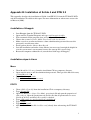
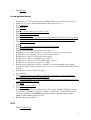
Appendix B: Installation of Scilab 4 and RTAI 3.3
1
Installation of Knoppix
Installation steps in Linux
Mesa
EFLTK
A new patched kernel
RTAI
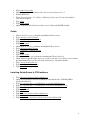
Scilab
Installing Scilab/Scicos & RTAI add-ons
Appendix C: Most important guide functions
New file
Load file
Save file
Export file
Add a control (for example the pushbutton control)
Delete a control
Edit a control
Add item to list box
Replace and resize items (for example x-coordinate slider moves)
Rename control
Appendix D: Graphical interface function of REF3
Main window
Edit trajectory window
Jogmode window
1
1
1
1
2
2
3
3
1
1
1
2
2
3
4
4
5
5
6
1
1
2
3
Appendix E: Sim function in Scilab
1
Appendix F: Contents of the CD
1
iii
1.
Introduction
With the increasing number of real-time applications an increasing want to cheap, reliable and
easy to use controller software originates. A very reliable software package currently on the
market is of course Matlab in combination with Simulink. This software provides a userfriendly interface to design controllers that in combination with the real-time workshop can
handle real-time processes. A disadvantage of Matlab is that it is a commercial software
package and it is therefore pretty expensive. As an alternative for Matlab, Scilab can be
found. This open source software package can be downloaded for free and when used in
combination with Real Time Application Interface (RTAI) it is possible to control real-time
applications.
Scilab works with Microsoft Windows and Linux. Regarding Microsoft Windows, only
Microsoft Windows CE is suitable with real-time processes, but this is a very expensive
software package too. For that reason Linux has been chosen as operating system.
In Maassen (2006) it has been approved that Scilab is a good alternative for Matlab showing
proper result with real time processes. Another conclusion was that Scilab is not as user
friendly as Matlab and that its user interface is a bit out of date. The main goal of this report is
to investigate if Scilab offers the ability of creating custom user interface and if so to explain
how it can be used. This explanation can be done by converting the REF3 user interface from
Matlab to Scilab.
As real-time application become more complex, different sensors and actuators need to be
integrated. By using all those different components in one single controller, different sample
rates are needed. The second goal of this report is to give a introduction to this so called
multi-rate tasking or distributed control.
This report consists of three sections. Since Maassen (2006) was written a new version of
Scilab and a new version of RTAI have been released. In the first part the differences between
Scilab 3 and Scilab 4 and between RTAI 3.2 and RTAI 3.3 are discussed including a new
installation guide.
The second part describes the user interface of Scilab and its tools and how to create custom
user interface. As an example the conversion of the REF3 user interface from Matlab to
Scilab is used.
As third a short introduction to multi-rate tasking is reported.
1
2.
Scilab 4 and RTAI 3.3
2.1
Major changes
2.1.1 Scilab 4
Since Maassen (2006) was written, two new versions of Scilab were introduced. Namely
Scilab 3.2 and Scilab 4. In this report, the newest version of Scilab has been used: Scilab 4.
This newest version will be the last using the ‘old’ graphics mode. So probably in newer
versions the graphics will be more up-to-date and more Matlab-like.
The major changes between Scilab 3 and Scilab 4 are also mostly graphical changes and
changes in functions to let them be more Matlab equivalent. Tools like Scipad and the Matlab
to Scipad converter are changed too. For example Scipad, the sci-file editor, is changed
especially in a graphical way. With different colours for different functions, statements and
variables the environment is more M-File Editor like.
A big missing in the list of changes between Scilab 3 and Scilab 4 is Scicos. This still uses old
graphics and a out of date user interface. For example drag and drop is still not supported and
in that way its development is far behind in comparison with Simulink. Nevertheless the
control capabilities are tested in Maassen (2006) and the overall conclusion is that Scicos is a
good alternative for Simulink. Newer versions will be more user friendly hopefully.
For a full list of changes between Scilab 3 and Scilab 4 see appendix A.
2.1.2 RTAI 3.3
Not only Scilab has changed, also the Real Time Application Interface (RTAI) has been
developed. The newest version is RTAI 3.3 were RTAI 3.2 was used in Maassen (2006).
Regarding the change log included in the installation file a lot has changed in the new version.
Most changes are bug fixes and implementations to derive better stability. In general a lot has
changed in the core files, but the user won’t notice the difference. In this report RTAI has not
been used very often, so there has not been made a deep investigation in the possibilities of
the new version of RTAI.
For a full list of changes between RTAI 3.2 and RTAI 3.3 see the change log included in the
installation file on the CD.
2.2
Installation
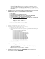
The installation of Scilab 4 and RTAI 3.3 has not changed a lot in comparison with Scilab 3
and RTAI 3.2. Just like described in Maassen (2006) the installation consists of three steps.
First a compatible Linux version has to be installed, in this report the Knoppix v.0.3.19.12 has
been used. This version is included in the TUeDAX DVD (Linux Live DVD for TUeDACS
2
QAD/AQI devices) version 3.2.2. In Maassen (2006) an older version of Knoppix was used,
but the installation and use of the newer version is exactly the same as the old.
Secondly the kernel needs to be patched in order to install RTAI. A new patch is used, but the
installation steps are the same. First install Mesa and EFLTK and then patch the kernel.
Finally RTAI 3.3 and Scilab 4 need to be installed. These installation steps are also exactly
the same as in Maassen (2006).
Be aware that the following steps need to be adapted in order to install everything:
• Everywhere replace linux-2.6.10 by linux-2.6.15
• Everywhere replace rtai-3.2 by rtai-3.3
• Everywhere replace linux-2.6.11-fusion-0.7 by linux-2.6.12.6-fusion-0.9.1
• Everywhere replace scilab-3.1.1 by scilab-4.0
In appendix B the installation steps are adapted as written above. Only the installation steps
are copied, so for more information or error solutions see Maassen (2006).
2.3
Solutions to known issues and problems
In Maassen (2006) already a couple issues were mentioned regarding the installation and
usage of Matlab, Scilab and Linux. The installation errors can occur with the new installation
too, but no more errors were discovered while installing the new versions. Nevertheless a
couple new errors were discovered during usage of Matlab, Scilab and Linux.
2.3.1 Matlab
•
Problem: start-up error when trying to start Matlab from within a console window.
Matlab starts in console window, displaying following error:
Xlib: connection to ":0.0" refused by server
Xlib: No protocol specified
Xlib: connection to ":0.0" refused by server
Xlib: No protocol specified
Warning: Unable to open display :0.0, MATLAB is starting
without a display.
You will not be able to display graphics on the screen
•
Solution:
o Leave Matlab by typing exit
o In the console type exit to exit super user mode
o Enter xhost + in the console
o Go back to super user mode by entering su and password
o Type matlab to start Matlab
o Now Matlab will start in its own window
•
Problem: when using Matlab Symbolic Toolbox the following error might be
displayed:
3
??? Invalid MEX-file
'/usr/local/matlabr14sp2/toolbox/symbolic/maplemex.mexglx':
/usr/local/matlabr14sp2/bin/glnx86/libmaple.so: symbol errno,
version GLIBC_2.0 not defined in file libc.so.6 with link time
reference.
•
Solution: this issue is the result of a conflict between the Linux kernel 2.4.2 and the
MAPLE function, and can be resolved by following the steps below:
o
o
o
o
o
Close Matlab
Go to directory /usr/local/matlabr14sp2/bin
Right-click file matlab and select KWrite from the Open With menu.
Scroll down until you see arg0_=$0 probably at line 166
Insert export LD_ASSUME_KERNEL=2.4.1 above this line, it will look like
this:
export LD_ASSUME_KERNEL=2.4.1
arg0_=$0
o Now save and close the file and restart Matlab
•
•
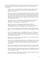
Problem: custom Simulink models won't work
Solution: be sure that the matlab paths are set correctly
o Choose Set path from the File menu
o Choose Add with subfolders and repeat this step until all of the following are
added:
/usr/local/matlab6p1/toolbox/local
/usr/local/matlab6p1/rtw/
/usr/local/matlabr14sp2/toolbox/qadscope
/usr/local/matlabr14sp2/toolbox/wintarget
/usr/local/matlabr14sp2/toolbox/diet
/usr/local/matlabr14sp2/toolbox/pizza
/usr/local/matlabr14sp2/toolbox/printer
/usr/local/matlabr14sp2/toolbox/demo01
/usr/local/matlabr14sp2/toolbox/minipato
/usr/local/matlabr14sp2/toolbox/pato
/usr/local/matlabr14sp2/toolbox/ref3ma
o Choose Save and Close
•
Problem: testref3 displays the following error:
Error evaluating 'OpenFcn' callback of Ref3 block (mask)
'edit_part/S-Function'.
Undefined function or variable "irepeat".
•
Solution: before starting testref3 type global irepeat or don't use testref3, but
ref3sa_template by typing ref3sa_template.
4
2.3.2 Scilab
•
•
Problem: help browser doesn't work.
Solution:
o Exit Scilab
o Download file man-eng-scilab-4.0.tar.tar from www.scilab.org
o Untar all files from the folder man-eng-scilab-4.0 in man-eng-scilab-4.0.tar.tar
to /usr/local/scilab-4.0/man/eng/. Overwrite all files.
•
Problem: during RTAI Code generation in Scicos the following error might occur:
Sorry file name not defined in c block
•
Solution: click on all blocks in the scheme so that all blocks are opened once.
2.3.3 Linux
•
•
Problem: when for some reason Microsoft Windows is installed or reinstalled after
Linux was installed in a other partition, the start up grub menu won’t appear anymore.
Solution: A new installation of Microsoft Windows to another partition will overwrite
the Master Boot Record (mbr) so that the link to the grub menu is deleted. This can be
solved in the following way:
o Boot computer from TUeDAX DVD or another bootable Linux CD/DVD.
o Start a console window and type grub.
o In the grub command line type:
root(hd0,6) where hd0 represents the hard disk where Linux is installed
on and 6 represents the Reiserf partition.
setup(hd0)
quit
o Reboot the computer and grub is recovered.
5
3.
User Interface in Scilab 4
3.1
Scilab user interface
User interface is very important when creating programs and tools. The user needs to find his
way around easily. With the development of Scilab, at first, the user interface wasn’t the
biggest concern, but with new version being released, the user interface starts to more and
more ‘up to date’. Users used to work with Matlab can find there way around in Scilab too,
because the user interface is beginning to mimic Matlabs user interface. Not only the
graphical objects are becoming more and more the same, also functions, syntax and
statements are developing in a Matlab way.
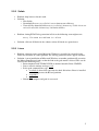
3.1.1 Main window
In general the user interface (gui) of Scilab is pretty familiar with the gui of Matlab. It’s also
possible to type commands in a command window. Just like Matlab there is a toolbar on top
of the window. This is a new feature first introduced in Scilab 4. But at first sight there are
also a couple differences. Scilab hasn’t got any separate windows like Matlabs command
history, current directory and workspace. Those features are nevertheless available in Scilab.
So is the command history accessible by typing gethistory, the result is a string matrix with all
commands typed. To clear the history simply select Clear History from the Preferences menu
or type resethistory in the command window. The menu’s mentioned are menu’s available in
windows, in Linux those menu’s are not available, but typing the commands will result in the
same.
It’s possible to view the current directory by typing pwd or getcwd and this directory can be
set by typing cd path or chdir(path), with path the path to which the working directory has to
be set to. It’s also possible to retrieve and change the current directory by clicking Get
Current Directory and Change Directory within the File menu, respectively.
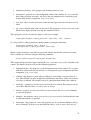
The workspace is available by typing browsevar or selecting Browser Variables from the
Application menu. A new window will appear with all the variables which are loaded in the
memory. To see all the variables in the command window it’s possible to type who.
Finally help is available by selecting Scilab Help from the ? menu or typing help function
name in the command window, where function name is a function from Scilab.
Figure 1: Scilab main window and variable browser
6
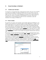
3.1.2 Scipad
Just like the m-file editor from Matlab, Scilab has a own sci-file editor named Scipad. This
editor can be loaded by typing scipad or selecting the Editor menu. This editor is very
familiar with the m-file editor. It’s possible to load sci-files into the editor and with different
colours different functions, keywords, statements and variables are indicated just like in the
m-file editor. In this sci-file editor even the short keys are the same, for example pushing the
F5-button will save and run the script. From within the File menu it is possible to select
Import Matlab file..., this function uses the mfile2sci tool to convert a m-file to a sci-file.
Later on more about this tool.
The syntax in sci-files is almost the same as in m-files. Be aware by using the conditional
execution if. In Scilab this statement has to be followed by a condition and the keyword then.
This is in contradiction with Matlab where then is not a valid keyword.
Another difference between m-files and sci-files is the fact that a sci-file can contain more
than one function. Every function needs to be closed by using the endfunction statement and
another function can be added to the sci-file just after this statement.
Figure 2: Scipad
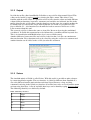
3.1.3 Scicos
The simulink mimic of Scilab is called Scicos. With this tool it is possible to make schemes
by connecting blocks together. The user interface is a little bit different from Simulink. It’s
also a bit different from the main window and from Scipad. Because a drag and drop
command is missing in the Scilab user interface all actions have to be accessed from the menu
or from using short keys. A list of available short keys can be found by typing %scicos_short.
The following short keys are defined by default:
Table 1 Short keys in Scicos
A
Align
D
Delete
C
Copy
M
Move
U
Undo
F
Flip
7
A
Align
O
Open/Set
S
Save
I
Get Info
R
Replot
L
Link
Q
Quit
By pressing one of these short keys, the operation is selected and is available for all blocks.
The white info line on top of the Scicos window displays information about which operation
is currently selected. It will take some time to get used to this kind of user interface and
probably it will change in future versions of Scilab. For more information see also Maassen
(2006).
Another difference between the user interface of Scicos and Simulink is the fact that Scicos
uses trigger signals that need to be implemented by putting a red clock in the scheme. This
clock needs to be connected to a red activation input on some blocks. These blocks are
triggered in a certain sample rate which is assigned to the clock. Most blocks have also black
in- or outputs, these are the data signals.
For more information about building RTAI code or an example how to build a Scicos-scheme
refer to Maassen (2006) or Bucher.
Figure 3: Scicos
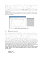
3.1.4 Graphics and figures
In Scilab, graphs and figures are not the same like in Matlab. In Matlab a graph is drawn into
a figure object. In Scilab these objects are separated. It is not possible to plot a graph into a
figure object. A graph is always plotted into a graphic window. These graphic windows have
there own menus and toolbars and look like the figures created by the plot statement in
Matlab. In these windows it is possible to zoom, save, load and edit properties. Most
commands available in the menu are the same as in Matlab.
The figure object in Scilab looks like the figure object in Matlab when no graph is plotted. In
this object controls like buttons or labels can be put. While in Matlab a graph and a control
8
can be put together into a figure, in Scilab it’s not possible to plot a graph into a figure object.
The figure objects are only designed to make custom user interface and graphs are always
plotted into graphic windows.
The best way to explain the difference between Matlab and Simulink at this point is to use the
following commands straight after each other: figure and plot(1). In Matlab firstly an empty
figure will be shown and then this figure is filled with the plot. In Scilab there will be shown
an empty figure too, but secondly a new window will be opened, a graphic window, which
displays the plot.
Difference between the figure and graphic window object is very important when creating
graphical user interface in Scilab. In the next paragraph is explained how to create custom
user interface in Scilab 4.
Figure 4: Graphic window and figure object
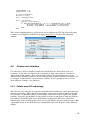
3.1.5 M-file to sci converter
When switching from Matlab to Scilab all m-files need to be adapted to sci-files. The syntax
of sci-files is almost the same as the syntax used in m-files. As mentioned before a big
difference is the use of a then statement. A bigger issue concerns the functions. Not all Matlab
functions are adapted to sci-files yet and even when they are adapted, not always the names
are familiar. To solve this problem a smart tool has been created, which can convert m-files to
sci-files. Unfortunately a couple bugs can appear when using this tool.
At first when converting a m-file a lot of warnings will appear. Far most warnings concern
syntax issues or function missing issues. The syntax warnings can be ignored mostly, because
syntax is almost the same. Function missing warnings are caused due to the fact that the tool
‘thinks’ that a function doesn’t exist in Scilab. But often this appears to be wrong because the
functions do exist. This is strange and can only be explained by suggesting that the tool isn’t
up-to-date. Furthermore this is not really a problem, because the warnings can easily be
ignored. Sometimes however the tool replaces the function by a Matlab equivalent which has
a mtlb_ prefix. Pretty often this is not necessary and the prefixes can be deleted.
Another error occurs when trying to convert a whole directory at once. This option should be
available, but doesn’t work. A simple workaround script can be written to convert a whole
directory at once:
mfilepath = '';
resultpath = '';
recmode = %f;
onlydouble = %f;
9
verbosemode = 0;
prettyprint = %f;
S = dir(mfilepath);
myfiles = S(2);
nof = size(myfiles);
for i = 1:nof(1)
myfile = myfiles(i);
if max(strindex(myfile,'.m')) == length(myfile)-1 then
mfile2sci(mfilepath + '/' + myfile, resultpath, ...
recmode, onlydouble, verbosemode, prettyprint)
end
end
This script is implemented in a sci-file and it can be found on the CD. For help on the input
variables see the help file of mfile2sci by typing help mfile2sci in the Scilab command
window.
Figure 5: Mfile2sci converter
3.2
Custom user interface
User interface is used to simplify certain tasks which otherwise would have been very
circuitous. At this time user interface on a computer is often represented by a window or
dialog with certain controls. These controls have different ways of handling and can do
different tasks. Within Scilab there are two different ways in which custom user interface can
be designed. Scilab itself has a user interface ‘toolbox’ and it’s possible to use tlc and tk
shared libraries to make a user interface.
3.2.1 Scilabs own GUI and dialogs
The first way is by using the user interface of Scilab itself. Scilab has a couple predefined gui
functions and dialogs. These functions and dialogs can be used to make a simple predefined
user interface. As mentioned before, Scilab makes a difference between figures and graphic
windows. Using this gui method it is not possible to create custom figures with own controls.
Everything is predefined with only a small number of properties that can be edited. The
following list shows all dialogs that can be accessed in Scilabs own user interface with a short
explanation of how to use them. For more information refer to the help files of the different
dialogs.
10
•
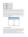
buttondialog - this dialog shows a message, icon and one or more buttons. The result is
the number of the button that has been clicked.
result=buttondialog(message,button1|button2|...|buttoni,icon)
Figure 6: Buttondialog
•
getvalue dialog - this dialog shows a window with different labels and texboxes. In all
the textboxes different values can be put. These values are the result of the dialog.
[ok,x1,x2,..,xi]=getvalue(message,labels,type,initialvalues)
Figure 7: getvalue dialog
•
progressionbar - this dialog shows a bar in which a red square ‘walks’ from the left to
the right and back. Every time the function is called, the progressionbar is updated.
This dialog can be used in order to indicate that the computer is busy.
winid=progressionbar(message)
progressionbar(winid,message)
//to update the bar
Figure 8: progressionbar
•
waitbar - this dialog is pretty much the same as the progression bar with one
difference. The bar in this dialog fills from the left to the right with a red square
instead off a ‘walking’ square. Dialog can be used to indicate the progress of a task the
computer is doing.
winid=waitbar(message)
waitbar(percent_filled,winid)
//to update the bar
Figure 9: waitbar
•
x_choices - this dialog shows different labels and different toggle boxes. Values can
be chosen from these toggle boxes. The result is a list of the chosen items.
11
result=x_choices(message,list_of_items)
Figure 10: x_choises dialog
•
x_choose - this dialog looks like the x_choices dialog, but this dialog shows one list
with items from which a item can be chosen. The result is the number of the chosen
item.
result=x_choose(items,message,custom_button)
Figure 11: x_choose dialog
•
x_dialog - this dialog shows a message with a textbox in which one value can be
given. This value is the result of the dialog.
result=x_dialog(message,initial_value)
Figure 12: x_dialog dialog
•
x_matrix - this dialog looks like the x_dialog but is meant to put matrices in.
result=x_matrix(message,initial_matrix)
Figure 13: x_matrix dialog
12
•
x_mdialog - this dialog is exactly the same as the getvalue dialog.
result=x_mdialog(message,labels,initial_values)
Figure 14: x_mdialog dialog
•
x_message - this dialog shows a message with custom buttons. The result is the
number of the button that has been pressed.
result=x_message(message,buttons1|button2|...|buttoni)
Figure 15: x_message dialog
•
x_message_modeless - this dialog shows a message and a ok button, just as the
x_message dialog. But when this dialog is shown, Scilab remains available for
commands.
x_message_modeless(message)
The biggest advantage of these dialogs is that they are easy to use and pretty fast to
implement, because there are just a small amount of properties. But that is also a disadvantage
when complex user interfaces need to be built. These dialogs have a lack of customization.
The only properties that can be set are all listened above. When complex user interface with
for example graphs are needed, these dialogs aren’t compatible anymore.
For example in Maassen (2006) a getvalue dialog was used for the REF3 block. It was
sufficient for the tests that had to be done, but when more complex signals are needed it is
way too user unfriendly. In that case a custom made dialog needs to be implemented. This can
also be done with Scilab in combination with the tlc and tk shared libraries.
3.2.2 GUI using tlc and tk shared libraries
When the standard dialogs of Scilab aren’t sufficient anymore, the shared libraries of tlc and
tk are the solution. With those libraries it is possible to make custom dialogs with controls like
buttons and labels. The commands that access these libraries are familiar with Matlab.
As mentioned before these libraries make use of the figure object, so firstly a new figure
needs to be called:
figure_hdl=figure(properties)
13
With figure_hdl the handle to the just created figure. This handle is needed when controls are
placed into the figure. The properties statement can contain a lot of different properties
listened below:
•
children - this is a vector with handles to the children of the figure window. All the
children are axes, which represent the outer border of the figure window. This
property is not used a lot.
•
figure_style - this represents the style of the figure. It can be set to old or new. When
set to old the figure uses the ‘old graphic mode’ of Scilab. This mode is actually only
used by Scicos and will no longer be in use in newer Scilab versions. Otherwise the
figure uses the ‘new graphic mode’ which is used by all other tools of Scilab, such as
Scipad. This property is not used a lot, it’s standard on new and it’s better to use the
‘new graphic mode’ in Scilab.
•
figure_position - this is a vector with the position of the figure in pixels. The vector
contains two values, the first value is the x-coordinate and the second the ycoordinate: [x, y]. This property is used almost always.
•
figure_size - this is the size of the figure window in pixels. Just like the
figure_position this is a vector containing two values, the first is the width and the
second the height: [width, height]. This property is used almost always too.
•
axes_size - this is the outer border of the figure window, the virtual graphic window.
This is also a vector containing two values: [width, height]. This property is not used a
lot.
•
auto_resize - this property can be set to two different values, on or off. When set to on
the axes_size is equal to the figure_size and when set to off the axes_size cannot be
changed. This property is just like the axes_size property almost never used. It’s best
to keep it just in it’s default state.
•
figure_name - this is the name of the figure. The name is on top of the figure window.
This property is used almost always.
•
figure_id - this is the figure identifier and cannot be set. This property is read-only and
is set at figure creation. When using more than one figure, this property can be used to
set the active figure window. It is a integer number the same as the handle of the
figure window.
•
color_map - this represents the colour map used by the figure. It is a matrix of colours
that can be used. The property is not used a lot and can be hold at default values best.
•
pixmap - this property sets the pixmap status. This is used to determine the way a pixel
is drawn on the screen, but there is no graphical difference in setting this property to
on or off. So this is never used.
•
pixel_drawing_mode - familiar with pixmap and also a property that handles the way a
pixel is drawn. So this property is also never used.
14
•
immediate_drawing - also a property for drawing and never used.
•
background - property to set the background colour of the window. It’s a vector with
three values between zero and 1, the first is the red component, the second the green
and the third the blue component: [red, green, blue].
•
user_data - this is to store and retrieve data into the figure structure, but not used very
often.
•
tag - here a identification name can be stored. This property is used a lot to retrieve the
handle of the figure window by using the command findobj.
These properties can be set when the figure is called, for example:
figure_hdl=figure('figure_position',[100 100],'tag','figure')
It’s also possible to change properties during runtime by using the following:
figure_hdl=findobj('tag','figure')
set(figure_hdl,'figure_position',[200 200])
Within a figure window it’s possible to put certain controls that handle certain user actions.
These controls are called by using the following command.
control_hdl=uicontrol(figure_hdl,properties)
This control will be put into a figure with handle figure_hdl and control_hdl is a handle to the
control. The handle can be used to use the following properties.
•
backgroundcolor - this property sets the backgroundcolor of the control. Use a vector
with three values between zero and one, a red component, green component and blue
component: [red, green, blue].
•
callback - this property is used when a callback is needed after a certain action of a
user. The callback can only be applied to pushbuttons and sliders. Other user controls
can’t have a callback. The property refers to a function which handles the callback.
•
fontangle - a property to set the style of text on the user control. This property can be
set to three different value’s: normal, italic or oblique.
•
fontsize - property to set the size of the text on a control. The size is set in fontunits,
see the next property.
•
fontunits - this property can be set to points, pixels or normalized and handles the units
in which the fontsize is specified.
•
fontweight - this property is a text style property too. It sets the font thickness of text
on a usercontrol. It can be set to four different value’s: light, normal, demi or bold.
15
•
fontname - also a property that sets a textstyle. This property sets the font of text on a
usercontrol.
•
foregroundcolor - just like background colour a style property that sets the colour of
the text on a user control. Also a vector containing three value’s: [red, green, blue].
•
horizontalalignment - property that sets the positioning of the text on a user control.
This property can be set to left, center or right.
•
listboxtop - this property can only be used with a listbox. It sets the item which will be
shown first in the list.
•
max - a property that sets the highest value of a control. This can be used with
checkboxes, sliders and listboxes. With checkboxes the value represents the value
when the checkbox is checked. With sliders this value sets the highest possible slider
position. With listboxes the property sets the possibility of multi-selection. If the
difference between max and min is greater then one multi-selection is enabled.
•
min - this property sets the lowest value of a control and can also be used with
checkboxes, sliders and listboxes. This property sets the value of checkboxes when
unchecked, the lowest possible slider position on sliders and the possibility of multiselection in listboxes.
•
parent - this is the handle of the control. By changing this property, the handle can be
moved from one figure to another.
•
path - read-only property that gives a string to the TK-path of the control. This
property is not used very often.
•
position - property to set the x- and y-coordinate and the width and height of the
control. Use a vector with four different value’s, the first two indicate the x- and yposition and the last two the width and height: [x, y, width, height].
•
sliderstep - only available with slider controls. This property sets the small and big
slider step size. The small step is when the user clicks on the arrow, the big step is
activated when clicked on the slide bar. Vector with two value’s: [small step, big
step].
•
string - this property sets the text on a user control. Within listboxes and popupmenu’s
this property can be a vector of strings separated by ‘|’.
•
style - this is the style of the user control. There are nine different styles available.
Pushbuttons are buttons that can be pressed and a callback is called. A radiobutton can
be checked or unchecked, only one radiobutton can be checked at the same time. A
checkbox is the same as a radiobutton, accept for the fact that those can be checked all
at the same time. An edit control is a editable field in which a user can put a string in.
A text control is a not editable label. With a slider the user can select a value by
sliding the bar. A frame is a border to separate different places in a figure window.
16
Listboxes are controls in which a list of strings is displayed. A popupmenu is a menu
which can be displayed when the user clicks.
Figure 16: all controls on one dialog
•
tag - identification string with which the control can be identified. Using findobj it’s
possible to retrieve the handle of the control.
•
units - this property sets the units used when setting the position property. Can be set
to points, pixels, normalized.
•
userdata - property to associate Scilab object to controls. Not used very often.
•
value - this is a the value of certain user controls. With checkboxes and radiobuttons
value is max when checked or min when unchecked. With listboxes and popupmenu,
value is a vector of strings. With sliders, value is the sliderposition.
•
verticalalignment - property that sets the vertical text position on a control. Can be set
using one of the following three strings: top, middle or bottom. It’s only possible to
use this property on text and checkboxes controls
Properties of controls can be set when called:
control_hdl=uicontrol(figure_hdl,'style','edit','tag','control')
But it is also possible to change properties during runtime:
control_hdl=findobj('tag','control')
set(control_hdl,'position',[5,35,200 200])
Finally it is also possible to place menu’s into a figure window. These menu’s are shown on
top of the window. Menu’s can be called using the following code:
menu_hdl=uicontrol(figure_hdl,properties)
menu_hdl=uidontrol(menu_hdl,properties)
The figure_hdl is the handle of the window in which the menu has to be placed. It’s also to
put a menu into another menu by using a menu_hdl instead of a figure_hdl. A menu object has
three different properties:
17
•
callback - this property is used to refer to a function which is called when the menu is
pressed.
•
label - this is the text displayed in the menu.
•
tag - just as mentioned before a identification string.
Combining all those different user interface objects it is possible to build complex and user
friendly dialogs. For an example refer to paragraph 3.4.
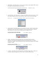
3.3
Guide
In Matlab it’s possible to create user interface using a tool called guide. This tool helps users
to create custom dialogs. It uses drag and drop to put controls on a figure object and it’s
possible to set different properties per control. In Scilab such a tool doesn’t exist, so to make
it easier to design a user interface a stripped version of the Matlab guide tool is created for
Scilab. With this tool, also called guide, it is possible to place different controls on a figure in
an easy way. Before this tool was created, the only way of designing a user interface was to
use trail and error. All the positions and sizes of all controls needed to be set before it could
be compiled. When compilation was ready it was necessary to run the file to see if the
controls were placed right. With guide it is possible to move and resize controls, seeing the
result directly.
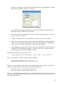
With guide it is possible to set the x- and y-coordinate, the width and height, and the name of
a control. So it’s not possible to set other properties like in Matlab, but these properties can
also be set in the sci-file which is exported by guide. Guide sets the background colour and
text alignment to default values, because in that way it is easier to place the buttons. These
properties can also be changed in the sci-file.
Figure 17: guide user interface
18
3.3.1 User manual
Using guide is pretty easy. First start the tool by typing guide in the command window. It’s
possible that Scilab doesn’t recognize the function and returns an error. Then the function
guide needs to be loaded into Scilab first using getf(path), with path the path to the file
containing the guide function. If the function is loaded retry starting guide. Be sure to use
only one guide at the same time, see paragraph 3.3.3 for more information.
When guide is started the main window will appear. Select New or Load from the File menu
to create or load a figure respectively. Selecting New will display a empty figure and load will
display a figure containing controls as saved last time.
A new menu will appear in the main window called Add and in the File menu the buttons New
and Load are replaced by Save and Export respectively. It is only possible to create or load a
new figure by restarting guide. In the listbox the name of the created or loaded figure is
shown. Select this and click Edit to load its position, size and name into the property fields.
Now it is possible to replace, resize and rename the figure window. It is also possible to add
some controls first and edit the figure window later on.
Controls can be added by using the Add menu. There are eight controls to choose from:
Pushbutton, Radiobutton, Checkbox, Edit, Text, Slider, Frame, Listbox. The popupmenu
control is missing because it’s position and size are set automatic when called. It is also not
possible to add a menu to the figure for the same reason. A menu is placed and sized
automatically too. These controls can be added manually when a sci-file is exported. When a
control is selected it will be added to the figure in the default position and size. Also a default
name is set to the control and displayed in the listbox. Guide also sets default background
colours and text alignment for easy positioning purposes. These values can be edited
manually when a sci-file is exported. The position and size of the controls can be edited by
selecting a control in the listbox and pressing Edit. The position, size and name will then be
loaded into the property fields.
When a figure or a control is loaded into the property fields its position can be changed in two
ways. Firstly sliding the x and y sliders will replace the control or by typing a value into the x
and y textboxes and pressing Check. In the same way the size of a figure or control can be
changed in two ways. By sliding the width and height sliders or by typing the correct value’s
into the width and height textfields. Renaming a figure or control can be done by entering a
string into the Name textbox and pressing the Rename button.
To delete a control, select the name from the listbox and press Delete. The name will
disappear from the listbox and the control will be deleted from the figure.
It is possible to save the user interface during design by selecting Save from the File menu.
The file will be save as a Scilab Graphical Interface file (*.sgi). In this file all positions, sizes
and names are saved. The file can later on be loaded as described above, it is not possible to
load a sci-file in guide.
To use the user interface created with guide, the whole graphical user interface needs to be
exported to a sci-file. This file contains the user interface script and can be loaded from within
Scilab. When this file is called the figure window created with guide will be shown containing
all the controls with their names, positions and sizes. Export a user interface by selecting
Export in the File menu.
Always close guide by selecting Exit from the File menu. So do not close guide by clicking
on the cross button in the right corner of the window. In that way guide is not correctly closed
and problems can occur when using it the next time.
19
3.3.2 Working of Guide
While programming guide some problems were discovered with the Scilab user interface. The
biggest issue that needed to be solved in order to make a workable guide tool was the fact that
Scilab isn’t compatible with drag and drop. So dragging a control from one window to
another isn’t possible.
The second problem is that not all controls use callback when clicked. So selecting a control
by clicking on the figure object isn’t possible. This would only be possible with a pushbuttonand slider control, because only these two controls use a callback function, but more controls
are needed.
These problems are solved together by using a listbox which displays the figure name and all
control names which are added to the figure. When a control is added to the figure object, it is
placed in the left lower corner with standard width and height. The control gets a name and a
tag which is the same. This name is also added to the listbox. Guide checks whether no other
control has the same name, so duplicate names aren’t possible and every control can be
identified by their own tag. When a control is selected it can be edited by clicking the edit
button, the position and size of the selected control will then be loaded into the property
fields. The selected control can be recognised by its unique tag. In the same way a control can
be deleted by clicking the delete button.
Saving and loading files is easily done by using the save and load and functions. Variables
can be saved using save(path, variable1,...,variablei) and loaded using load(path,
variable1,...,variablei), just like in Matlab.
Exporting a file is done by using the fprintf function. With this function it is possible to write
data into a file, just like in Matlab. When saving the file as sci-file it can be compiled and ran
in Scilab, resulting in a graphical user interface.
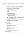
In appendix C the most important functions that control guide are mentioned.
3.3.3 Known bugs and issues
A couple issues were discovered using the guide tool:
•
Sliding the sliders to fast will effect in bad program behaviour. For some reason the
sliders aren’t able to use the callback fast enough when the slider is moved to fast.
When for some reason the slider moves in a strange way, it’s possible to click the
check button to reset the sliders or to click on the slider bar. In that way the sliders and
controls are reset to there actual position.
•
Be sure to use only one guide tool at the same time. Opening guide while another
window of guide was still running will result in unwanted behaviour. To start a new
design of a user interface close guide by clicking Exit in the File window and restart
the tool by typing guide in the Scilab main command window. It’s not possible to
design two different figures at the same time.
20
3.4
REF3 user interface example
In Maassen (2006) a couple blocks were designed to be able to use the TUeDACS QAD/AQI
devices with Scilab. One of that blocks was the REF3 block. This block was built to create
custom reference trajectories to use in control systems for real time devices. It was built in
Matlab/Simulink and Maassen (2006) describes how it was recently implemented in Scilab.
Everything works nicely, accept for the user interface. In Maassen (2006) a x_dialog (see
paragraph 3.2.1) was used as user interface for the input parameters. In Simulink a custom
user interface was used to retrieve those input parameters, but the implementation in Scilab
and especially Scicos is a bit different.
When a user clicks on a user defined block in Simulink a function is called. This function can
be set in the properties of the block. In Scicos it is possible to put user interface code in the
sci-file which handles the user events. Functions can be called from within this sci-file just
like the functions called in Simulink. For example in the REF3 sci-file, the x_dialog needs to
be replaced by custom user interface code to use a custom user interface. To implement the
user interface from Simulink into Scicos it is necessary to know something more about the
working of the REF3 user interface.
3.4.1 Working of REF3 user interface
The working of the REF3 user interface is pretty complex and it is not necessary to explain all
details but a short explanation is handy to understand how the implementation in Scilab has
been done.
To start the REF3 user interface in Linux in Matlab type testref3 in the main command
window. A simulink file will open with the REF3 block on. Double-click on the REF3 block
and the REF3 user interface will show up. A callback in the REF3 block properties calls a
function in Matlab which at his way shows a figure object saved in a fig-file created with
guide. All dialogs are fig-files created with guide and can be called from m-files.
It is possible that an error occurs when double clicking on the block, see paragraph 2.3 for
more information.
The REF3 main window shows a graph with the total trajectory and buttons like load, save,
new and accept. It is possible to add, delete or edit a part of the total trajectory by clicking
those buttons. When done a new window will appear with four graphs representing the
position, velocity, acceleration and jerk of the trajectory. Edit these parameters to change the
trajectory and click accept to save it. In the main window it is also possible to choose for
jogmode to create a jogmode signal.
The strength of the REF3 user interface is of course the graphs showing the user directly
changes in parameters. This is the core feature of the REF3 user interface and needs to be
implemented in Scilab. The working of the graphs in Simulink is pretty easy. With the
function sim it is possible to simulate a Simulink model and retrieve the different outputs. To
draw the graphs in the REF3 user interface, the REF3 Simulink model, using a s-function as
mentioned in Maassen (2006), is used. With the outputs, graphs can be drawn.
The s-function which is linked to a user-defined block in Simulink contains the code that
calculates positions, velocities, accelerations and jerks. In paragraph 3.4.2 it can be seen that
it’s useful to know how this function works, so a short explanation follows.
To retrieve the desired trajectory a position, velocity and acceleration like in figure 18 can be
plotted. This acceleration consist of a couple linear functions that describes the desired
acceleration for the trajectory. This plot can be separated into eight different zones, t0 to t8.
For each zone a linear function can be formulated. Integrating this functions once respectively
21
twice gives functions for velocity and position. Differentiating the acceleration functions once
gives the required jerk functions. When the functions are known it is possible to make a loop
over time from t0 to te. Within this loop check for every time which zone is active and use the
corresponding functions to calculate position, velocity, acceleration and jerk.
3.4.2 REF3 user interface in Scilab
Because the REF3 user interface already exists in Matlab, the mfile2sci tool is able to convert
all files from Matlab to Scilab. If a user interface doesn’t exist already, a new user interface
has to be made. Using the tlc and tk shared libraries a figure can be called to put controls on
as mentioned above. Of course it is also possible to use the guide tool to create graphic
interface. For a example of how to use figures and uicontrols see appendix D, where the
functions that create the user interface for the REF3 tool are described. Manually add
functions to the exported file to create a user interface. But in this case all files from Matlab
were converted. All functions were put into four different files, for each dialog a file is
created and one file for some main scripts used in all dialogs. After the conversion, when
trying to run the files for the first time errors will occur because not all functions are
converted correctly. The conversion of REF3 lead to a couple errors regarding missing
functions like sim and ginput.
As mentioned in paragraph 3.4.1 the core of the REF3 user interface consists of a couple
graphs which are drawn using the function sim in Matlab to simulate a Simulink model. This
function is one of the missing function in Scilab. There are two alternatives that can be used,
scicos_simulate and scicosim. Both function can simulate a Scicos scheme, but with
scicos_simulate the scheme has to be compiled first while scicosim can do a compilation
itself. So just replacing sim by one of this function would do the job, but it isn’t that easy.
These functions are very complex, the input and output parameters are hard to understand
structures containing hundreds of value’s. This wouldn’t have been a problem if the
documentation had been up to date and more detailed. Trying to use one of these functions
failed, so another way had be figured out. At this point the knowledge of the working of the
REF3 user interface becomes useful.
The solution to this problem is to write a sci-file containing the part of code that calculates the
position, velocity, acceleration and jerk. The working of this part of code is already explained.
Because no s-function can be simulated the part of code needs to be converted to scilanguage. In this way, the function can be called giving the opportunity to make graphs. To
see the full function which is created in Scilab refer to appendix E.
The REF3 user interface in Matlab uses callback functions in textboxes to auto update the
graphs. In Scilab call-backs are only allowed with buttons and sliders, so graphs can not be
updated automatically. This is not really a problem, but every time a value is entered in a
textbox, the check button needs to be pressed to update the graphs. There is no other solution
to this problem.
Another problem is that in Matlab, buttons can be disabled and enabled. This function ability
is missing in Scilab, so all the buttons can be clicked at any time. This can cause problems,
but there is no solution for this problem. See paragraph 3.4.3 for more details.
When editing a certain part of the trajectory, it is necessary to select the part by clicking in the
graph. In Matlab the function ginput is used, but Scilab hasn’t got this function. Nevertheless
22
a pretty familiar function called xclick is able to do the same. The function must be used in the
following way:
[c_i,c_x,c_y,c_w,c_m]=xclick()
With c_i the button that is pressed or clicked, c_x and c_y the coordinates of the position of
the mouse click, c_w the window number where the click has occurred and c_m the number of
a menu, when clicked in a menu. See Scilab help for more information.
In paragraph 3.1.4 has been mentioned that graphs can not be plotted into figures. This brings
a certain deficiency in programming REF3 user interface. A communication between the
figure and graphic window needs to be implemented. Fortunately this is not really hard to do.
When a graphic window is called a handle is saved in a variable. When this variable is first
declared as global, it can be used in every function. So when something needs to be plotted in
a graphic window, just call the handle and the plot can be done.
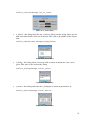
Because the REF3 user interface needs to be implemented in a sci-file created in Maassen
(2006) a pause statement needs to be implemented just after the main dialog is loaded.
Otherwise the main dialog would appear, but the sci-file from Maassen (2006) would still be
running and cause errors because no trajectory is created yet. This sci-file needs to be paused
until the accept button is clicked and a trajectory is designed. When a trajectory is designed
the accept button can be pressed, all windows will close, but to return to the Scicos scheme
the return statement needs to be entered in the main Scilab window.
At last the syntax needed to be adapted. As mentioned in paragraph 3.1.5 the mfile2sci tool
isn’t up to date and here and there some syntax errors were discovered. Furthermore no big
adjustments had to be made.
Figure 18: REF3 main window, REF3 edit trajectory window and REF3 jogmode window
23
3.4.3 Known bugs and issues
Because not all function could be translated as mentioned above, a couple issues and bugs can
appear:
•
Enabling and disabling controls is not possible in Scilab so when the edit trajectory or
jogmode dialog is shown it is not possible to use the main dialog. In Matlab this was
resolved by disabling all buttons on the main dialog. When accidentally pressed a
button on the main dialog while another dialog was already loaded, just close all
dialogs and restart REF3. Otherwise the tool doesn’t work correctly and errors may
occur.
•
Scicos is still using the old graphic mode while the rest of Scilab is using a new
graphic mode. In this old graphic mode it is not possible to position and size graphic
windows. The result is that a graphic window is positioned and sized with default
value’s and the windows are displayed across the screen which can be frustrating. In
the new graphic mode positioning and sizing graphic windows is implemented, but
until Scicos will use the new graphic mode, this problem remains undissolved. This
version of Scilab is the last using the old graphic mode, so probably this issue will be
fixed in the next version.
•
For some reason Scilab doesn’t always load all functions. To resolve this problem use
the getf(path) to load all function in a sci-file. The easiest way is to put the four files
containing all functions in the working directory, which by default is /home/username
with username the name of the active user in Linux. Then it is namely possible to only
use the name of the file in getf instead of the entire path.
24
4.
Multi-rate tasking in Scilab 4
In many systems different sensors and actuators are used. For example the soccer playing
robots such as used in the Robocup have camera’s to visualize their environment and a couple
motors to drive. In such systems the camera’s typically work at 20 or 30 frames per second.
Therefore the sample rate which controls the camera’s doesn’t need to be higher than 20
Hertz. On the other hand the control for the motion typically uses a sample rate of 1000 Hertz.
So when both controls systems are integrated, it is not necessary to use a sample rate of 1000
Hertz for the visualization, but a multi rate system can be designed. The robots in the
Robocup use therefore two different controllers working at 20 and 1000 Hertz for the
visualization and motion respectively. Those controllers are created with Simulink.
Communication between those two controllers takes place with so called shared memory.
Another application where communication between different tasks is necessary is when
distributed control is desirable. Distributed control are also controllers separated over
different tasks, these tasks can run on a local computer or on a network of more than one
computer. The big question is if multi rate systems can be designed with Scilab.
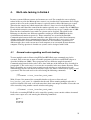
4.1
General notes regarding multi-rate tasking
To start multiple tasks in Linux using RTAI and RTAILab some commands need to be
executed. First create two or more executable programs with Scicos and RTAICodegen as
described in Maassen (2006). These programs may use different sample frequencies.
Communication between those tasks can be done with one of the different ways described in
paragraph 4.2. The easiest way is to create the executables in the users home directory. When
those executables are created, open as much console windows as tasks that need to run
simultaneously and be sure that in all windows super user mode is turned on by typing su and
a password. The first task needs to be called using the following commands:
./rl
./filename1 -n host_interface_task_name1
With filename1 the name of the executable that has to be run as first task and
host_interface_task_name1 is a identifier for the task. When running multiple tasks this is
needed to identify each task, so all tasks must have their own unique identifier. Next tasks can
all be started by using another console window and typing:
./filenamei –n host_interface_task_namei
If all tasks are running RTAILab can be started by opening a new console window in normal
mode, not as super user, and entering the following commands:
xhost +
su
password
xrtailab
25
With password the password of your account. The program is started. To connect to a task
select Connect to target in the File menu. A dialog will appear with standard value’s. Change
the value for Task identifier into the name of the identifier of the task that needs to be scoped
and click Ok. RTAILab is now connected to the selected task. To scope more than one task, it
is possible to start a new RTAILab or to disconnect by clicking Disconnect in the File menu
and reconnecting to another task using another Task identifier. Running multiple RTAILabs at
the same time requires a lot of cpu and as a result the computer may become unstable or
RTAILab isn’t updated fast enough anymore. It is better to reconnect to another task.
To stop a task it is possible to select Stop realtime code in the RTAILab toolbar or by pressing
ctrl-c in the console window of the task that has to be quitted.
4.2
Multi-tasking possibilities
According to Yaghmour a couple different communication ways can be created by using
RTAI. These ways are shortly explained below as an introduction to multi-rate tasking and if
tested a recommendation is made whether that way can be used in multi-rate tasking. Tests
are done with mailboxes, semaphores and I/O, because these methods are integrated into
blocks in RTAI by default. The other ways are not tested yet. In every test the sender is
sampled at ten Hertz and the receiver at one hundred Hertz. A sinus signal has been send from
sender to receiver. To visualize the signals in RTAILab one scope is used in each task.
Because a single task can’t contain two different sample rates, there are always two tasks
created and ran simultaneously.
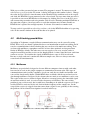
4.2.1 Mailboxes
Mailboxes are particularly designed to let two different computers interact with each other,
but can also be used on one single computer to communicate between tasks. This type of
communication works just like a mailbox. A task can send data to a buffer and another task
can read the data from the buffer. Within RTAI there are blocks which can send and receive
data through mailboxes. In figure 19 the schemes that are made to test mailboxes can be seen.
The results of the tests are shown in figure 20 and are a strange because the sinusoidal signal
of one Hertz which is send, is received with a frequency of ten Hertz. The cause of this
problem is not yet discovered, but it could have something to do with the scopes used. Scopes
used by RTAI are activated by the red clock with the frequency of the sample rate. So the
scope of the receiver is triggered ten times more than a signal is sent, probably is that causing
the problem. All in all more investigation is needed in this way.
Figure 19: Scicos schemes using mailbox send and mailbox receive
26
Figure 20: results of mailbox communication, send and receive side respectively
4.2.2 Messages and RPC
With this method it is also possible to send and receive data between different computers, but
can also be used on a local computer. Like mailboxes a sender sends data, but in this case, it’s
not stored in a buffer but send directly to the receiver. Therefore the receiver needs to be a
active task and waiting to receive data. Unlike mailboxes the data that is send has a fixed size.
There are no blocks in RTAI that can handle messages and RPC so no tests are executed.
4.2.3 Semaphores
Data can also be sent using a semaphore. This method creates a channel between two task and
data can be sent over this channel when the tasks want to synchronize. RTAI contains two
blocks which use semaphores to communicate. In figure 21 the schemes are displayed that
have been used to test. With this method the data is sent correctly when the same sample rates
are used in both tasks. But when different sample rates are used, the tasks become unstable
and plots in RTAILab will freeze. It is also possible that the whole system freezes. To
conclude semaphores are not working with different sample rates and so can not be used in
multi-rate systems.
Figure 21: Scicos schemes using semaphore send and semaphore receive
4.2.4 FIFO
This method is used to put data parts into a buffer. Unlike mailboxes, where all data from the
buffer can be read, this method uses first-in-first-out. This method is particularly used to
communicate between real time tasks and the user space. It handles communication between
real-time tasks and tasks which are not real-time. Although RTAI library contains one block
27
which handles communication with FIFO, this method was not tested because all tasks must
be real-time in this case.
4.2.5 Shared memory
Just like with the Robocup robots it is possible to use shared memory as communication
method. With this method multiple tasks are sharing the same memory region and all tasks
can access variables stored in the memory. This type of communication can also be used with
real-time and user space tasks. This method has not been tested.
4.2.6 I/O
With this communication way RTAI is not used. The blocks that handle this method are in a
standard library of Scicos. I/O can only be used on a local computer, it is not possible to
connect different computers with each other. The schemes that were used during testing are
displayed in figure 22. The result from RTAILab are the same as with the mailboxes in figure
20. The frequency of the signal is ten times higher on the receiver side than on the sender
side. To check if this could have something to do with the RTAI scopes a new model is built,
shown in figure 23. This model uses scopes from the Scicos library which are not triggered by
an activation signal. The results are displayed in figure 24 and as can be seen, the frequency is
the same in both scopes. Also it can be seen that the receive scope is drawn in more sharp
edged way. This is caused by the higher frequency and these results were expected at first.
This strengthens the first idea, but it is not yet a fact that the problem is caused by the scopes
and more research will be needed.
Figure 22: Scicos schemes using I/O send and I/O receive
Figure 23: Scicos schemes using I/O send and I/O receive without RTAI scopes
28
Figure 24: results of send and receive side respectively without using RTAI scopes
29
5.
Conclusions
The differences between Scilab 4 and Scilab 3 and between RTAI 3.2 and RTAI 3.3 are pretty
small. Especially with RTAI only some core changes were made. In Scilab 4 the user
interface is changes, so that it becomes more user friendly and Matlab-like. Also some
functions are adapted so that these can be used in a same way as in Matlab. Unfortunately
Scicos is not updated and its user interface is still out of date and user unfriendly, but this will
be solved in the next version probably because this version is the last using the old graphic
style. Within the installation not that much is changed, although a couple new errors were
discovered and solved.
Although the user interface of Scilab and especially Scicos is not as user friendly as Matlabs,
there are a few ways to create custom user interface. By using Scilabs own user interface
some predefined dialogs can be used or by using tlc and tk shared libraries own dialogs can be
created. A lot of functions that handle custom user interface with tlc and tk shared libraries are
the same as in Matlab so the mfile2sci tool can be used to convert m-files to sci-files if the
user interface already exists in Matlab. Otherwise it is possible to create graphical user
interface manually or by using the guide tool which is created to simplify the graphics design
process.
The different ways to create user interface in Scilab are all investigated and discussed in this
report and therefore this goal is achieved. Also the objective to implement a user friendly
REF3 user interface into Scilab is achieved. The graphic user interface of REF3 in Scilab
looks like Matlabs as much as possible.
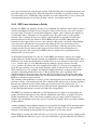
Finally a short introduction has been made to multi-rate tasking. Different ways of
communication between different tasks are described. Some of this ways are tested and
recommendations are given if it is possible to create multi-rate systems using that kind of
communication way. Some more investigation is needed to ultimately create a multi-rate realtime application in Scilab, but all in all it is possible.
The overall conclusion is that Scilabs user interface is pretty extensive and looks like Matlabs.
Multi-rate tasking is probably possible with Scilab and RTAI, but a lot of investigation needs
to done.
30
6.
References
6.1
Books and reports
H. Bruyninckx, (2002), Real-Time and Embedded Guide, K.U. Leuven - mechanical
engineering, Belgium
R. Bucher, Lorenzo Dozio and Paolo Mantegazza, (publication year unknown), Rapid Control
Prototyping with Scilab/Scicos and Linux RTAI, SUPSI and DIAPM
R. Bucher, (publication year unknown), Interfacing Linux RTAI with Scilab/Scicos, University
of Applied Sciences of Southern Switzerland
R. Bucher, S. Mannori (publication year unknown), Using Scilab/Scicos with RTAI-Lab,
University of Applied Sciences of Southern, Switzerland and proXima electronics, Italy
R. Djenidi, C. Lavarenne, R. Nikoukhah, Y. Sorel and S. Steer, (1999), From Hybrid System
Simulation to Real-Time Implementation, INRIA
M.G.J.M. Maassen, (2006), Scicos as an alternative for Simulink, Technical University of
Eindhoven, Holland
R. Nikoukhah and S. Steer, (publication year unknown), Scicos - A Dynamic System Builder
and Simulator User’s Guide
G. E. Urroz, (2003), Scilab scripts, functions, and dairy files - a summary
G. Vernaeve, (2000), Cursus C, Zeus WPI - workgroup informatics
K. Yaghmour, (publication year unknown), The Real-Time Application Interface
Multiple writers, Scilab help (2006), INRIA
6.2
Websites
Scilab 4 Features, http://www.scilab.org/download/features/scilab40.php
Scilab documentation (4.0 version), http://www.scilab.org/product/man-eng/index.html
31
Appendix A: Major changes between Scilab 3 and Scilab 4
Source: http://www.scilab.org/download/features/scilab40.php
•
Graphics:
o Graphical entities (objects) have been extended with a particular effort on:
The Axes entity with respect to change of coordinates (logscale enable,
axes inversion in 2D and 3D) and graduation display.
Versatile Title and labels entities in 2D and 3D.
3D object merge and zoom
Rotation of text entities
Save and load of all graphical entities
o New functions have been defined to mimic their Matlab equivalent:
plot
surf
mesh
bar, barh and barhomogenize
pie
o Graphical Environment improved and extended:
Manipulation of the hierarchy of the entities has been made easier
thanks to a hierarchy browser.
A toolbar has been added to the graphic windows, the function toolbar
can be used to set or unset it. (Windows specific)
o Graphic window Events (mouse, keyboard,...) handling have been improved
and extended:
Click, double-click, press, release, move
Key press and release, with or without Shift and Ctrl modifiers.
o xs2bmp and xs2emf functions added to export graphics under bmp and EMF
(Enhanced Meta File) formats. (Windows specific)
o colour bar function added
•
Numerical computation:
o Sparse operations and functions like real, imag, matrix, spones revisited to
improve efficiency
o Bessel functions extended to work in the complex case (using Slatec routines)
Incompatibilities: The semantics of besseli, besselj, besselk and bessely
functions has been changed and extended.
The oldbesseli, oldbesselj, oldbesselk and oldbessely correspond to the old
obsolete semantics.
o New version of linpro and quapro. Thanks to Cecilia Pola.
o bvodeS function added to solve differential equation with boundary value.
Thanks to Rainer Von Seggern.
o detrend function added to remove constant, linear or piecewise linear trend
from a vector
o Interface with Excel (Functions to read Excel files).
•
Matlab to Scilab converter:
o Translate paths function improved to allow conversion on an entire toolbox
propagating inference through toolbox functions.
1
o The set of translated function has been extended in particular with the basic
graphic functions.
o Scilab function sum, prod,... extended to the "first non singleton" matlab
semantics to improve readability and efficiency of translated code.
o Try catch construct added to Scilab for a better translation.
•
Scipad editor:
o A debugging tool is now available
o Drag and drop is now supported
o Split a Scipad window
o Print file from Scipad is now available
o Scipad is easily localized (See "Adding translations..." in the Scipad Help
Menu).
Today English, German, French, Swedish, Polish, Norwegian and Italian
languages are supported
o User settings and text colours are now configurable and saved across editing
sessions
o Colorization of strings rewritten - now supports strings on continued lines
o Colorization of files launched in the background, with progress bar.
o Quick access in the file menu for recently opened/saved files
o Identification of Scilab predefined variables and library functions in Scilab
scripts
o Miscellaneous file management improvements: read-only flag, absolute
pathnames to files, pruned pathnames display, revert to saved feature, MRU
(Most Recently Used) list.
o Keyword completion added, keyword list now completely dynamical
o Undo/Redo rewritten
o Go to... functions rewritten and expanded
o Find/Replace rewritten, includes find files, find in files, find in multiple
buffers, find in selection only, find full word
o Creation of XML help page templates and xml to html compilation available
from within Scipad
•
Syntax:
o try-catch instruction added to improve programming with error control.
•
Other improvements:
o Configure adapted to Linux 64bit architectures
o Use tcltk 8.4.12 - TCL interface has been totally rewritten (for better error
detection and better data transfer). ScilabEval improve to handle synchronism.
o Memory improvements under Windows platforms (particularly the
management of virtual memory or swap file)
o Exception management added under Windows version
o Windows platforms with:
Intel C Compiler 9.0
Intel Fortran 9.0
o The source files have been updated to optimise the compiled version built with
VC6 tool
Please note that the Windows binary version provided on our Web site is built
with .NET
2
o Improvement of the integration of Visual Studio Compiler to the dynamic
links: findmsvccompiler() and configure_msvc() macros have been added
o Integration of the ATLAS library (specific Windows version).
During the installation of Scilab, dynamic library (Atlas.dll) is automatically
chosen according to the CPU detected
See details in the Atlas.spec file under scilab\bin directory
o For advanced users: Scilab can be used with Atlas library on all platforms by:
downloading Atlas library sources,
compiling Atlas sources,
compiling Scilab sources with the following configure option : --withatlas-library=ATLAS_LIB_DIRECTORY
(see /configure --help)
o Java interface written to allow calling Scilab computational engine from Java
o Font rotation is now possible under Xwindow
o SCI and HOME are redefined if not correct ( Bug 1488 Only for Windows )
o home variable (%HOME%) defined under Windows: c:/Documents and
Setting/USER
o New environment variable SCIHOME:
Under Windows: %HOME%\Scilab\SCILAB_VERSION
Under Linux: $HOME/USER/.Scilab/SCILAB_VERSION
o Function what() has been rewritten : alphabetical sort, print modified
•
New primitives:
o clipboard (specific Windows)
o perl
o calendar
o mkdir
o rmdir
o copyfile
o sleep
o getos
o setenv
o toprint("file")
o getmemory()
o getshortpathname (specific Windows)
o getlongpathname (specific Windows)
o toolbar (specific Windows)
o hidetoolbar (specific Windows)
o console (specific Windows)
o mcisendstring (specific Windows)
o banner
o winqueryreg (specific Windows)
o xls_open
o xls_read
•
Please note:
o "xgetmouse", "eventhandler" event set extended to click, double-click, <Ctrl>
Key. See more details in xclick and xgetmouse on line help.
Warning: Because of distinction of click events, some users' scripts can have a
different behaviour.
3
To make it work as before please check and modified test on events as follow:
supposing that button contains the value returned by xclick (left most
argument) or xgetmouse (third component of returned vector) then replace test
like:
button==0 by or (button==[0,3])
button==1 by or (button==[1,4])
button==2 by or (button==[2,5])
4
Appendix B: Installation of Scilab 4 and RTAI 3.3
This appendix describes the installation of Scilab 4 and RTAI 3.3 from the TUeDACS DVD
and the installation CD added to this report. For more information or when errors occur refer
to Maassen (2006).
Installation of Knoppix
•
•
•
•
•
•
•
•
Start Knoppix from the TUeDACS DVD
Open console (Terminal Program) and type: sudo knoppix-installer
Wait a moment till the program starts and configure a new installation
Choose the system: beginner: Multi-User System with hw-detection
Make a new user account and choose a short administration password because this
password is needed more often
Install grub to the mbr: Master Boot Record
Start the installation and make a boot diskette (not necessary but might be helpful in
case the system won’t start anymore because the start-up file is messed up)
Restart the computer without the cd (start the hard disk copy of Knoppix)
Installation steps in Linux
Mesa
•
•
•
•
Untar MesaLib-6.3.2.tar.gz from the installation CD in a temporary directory
Open console enter su and the administration password. Then go to the Mesa directory
(cd /tmp/Mesa-6.3.2)
Type make linux-x86-static
Type make install (enter-enter-enter)
EFLTK
•
•
•
•
•
•
•
Untar efltk-2.0.5.tar.bz2 from the installation CD in a temporary directory
Type cd /tmp/efltk
Open File Manager – Super User Mode, go to /tmp/efltk and open the properties of
efltk-config.in. Open the permissions tab and be sure that all permissions are set to
Can Read & Write and that Is Executable is checked
Type ./efltk-config.in --prefix=/usr/local –multithread
Type ./emake
Type ./emake install
Add /usr/local/lib to the file /etc/ld.so.conf (already done when using the TUeDAX
cd)
1
•
Type ldconfig
A new patched kernel
•
•
•
•
•
•
•
•
•
•
•
•
•
•
•
•
•
•
•
•
•
•
•
•
•
•
•
•
•
•
•
Untar linux-2.6.15.tar.bz2 from the installation CD to /usr/src/linux-2.6.15-rtai-3.3
Untar rtai-3.3.tar.tar from the installation CD to /usr/src/rtai-3.3
Type cd /usr/src
Type rm linux
Type y
Type ln -s /usr/src/linux-2.6.15-rtai-3.3 linux
Type ln -s /usr/src/rtai-3.3 rtai
Type cd /usr/src/Linux
Type patch -p1 < /usr/src/rtai/base/arch/i386/patches/hal-linux-2.6.15-i386-r9.patch
Type cp /usr/src/linux-2.6.12.6-fusion-0.9.1/.config /usr/src/linux-2.6.15-rtai-3.3
Type rm /usr/include/asm
Type y
Type ln -s /usr/src/linux/include/asm-i386 /usr/include/asm
Type make menuconfig
Change General setup >> Local version to -rtai-3.3
Exclude Processor type and features >> Symmetric multi-processing support
Include Processor type and features >> Preemptible Kernel
Exclude Device Drivers >> Parallel Port support
Exclude Device Drivers >> Multi-device support
Exclude Device Drivers >> Fusion MPT device support
Exclude Power management options >> APM
Include Power management options >> ACPI >> needed functions (for a laptop
include AC Adapter, Battery, Button, Fan, Processor, Thermal Zone and other needed
features).
Include File systems >> Reiserfs support
Save and exit
Type cp /usr/local/gcc-3.2.3/lib/gcc-lib/i686-pc-linux-gnu/3.2.3/include/stdarg.h
/usr/src/linux-2.6.15-rtai-3.3/include/stdarg.h
Type cp /usr/src/linux-2.6.15-rtai-3.3/include/mca-legacy.h /usr/src/linux-2.6.15-rtai3.3/include/linux/mca-legacy.h
Type make
Type make modules_install
Type make install
Add the new kernel to /boot/grub/menu.lst. Use as title ‘Debian GNU/Linux, kernel
2.6.15-rtai-3.3, Default’, as root use ‘(hd0,6)’, as kernel use ‘/boot/vmlinuz-2.6.15rtai-3.3 ro ramdisk_size=100000 init=/etc/init lang=us acpi=off noapic noapm
xmodule=fbdev nomce quiet vga=791’
Reboot using the new kernel
RTAI
•
Type cd /usr/src/rtai
2
•
•
•
•
•
•
•
Type make menuconfig
Change General >> Installation directory to /usr/realtime-rtai-3.2
Include RTAI-Lab
Type cd /usr/local/gcc-3.2.3/lib/gcc-lib/i686-pc-linux-gnu/3.2.3/include/stddef.h
/usr/include/stddef.h
Type make
Type make install
Open /etc/profile and add /usr/realtime-rtai-3.2/bin to the PATH variable
Scilab
•
•
•
•
•
•
•
•
•
•
•
•
•
•
•
Untar tcl8.4.11-src.tar.gz from the installation CD to /usr/src
Type cd /usr/src/tcl8.4.11/unix
Type ./configure -enabled-shared
Type make
Type make install
Untar tk8.4.11-src.tar.gz from the installation CD to /usr/src
Type cd /usr/src/tk8.4.11/unix
Type ./configure -enabled-shared
Type make
Type make install
Untar scilab-4.0-src.tar.tar from the installation CD to /usr/local/
Untar all files from the folder man-eng-scilab-4.0 in man-eng-scilab-4.0.tar.tar from
the installation CD to /usr/local/scilab-4.0/man/eng/. Overwrite all files.
Type cd /usr/local/scilab-4.0
Type ./configure -without-java
Type make all
Installing Scilab/Scicos & RTAI add-ons
•
•
•
•
•
•
•
•
•
•
Type cd /usr/src/rtai/rtai-lab/scilab/macros
Open /usr/src/rtai/rtai-lab/macros/Makefile and edit the line: SCILAB_DIR =
/usr/local/scilab-4.0
Type ln -s /usr/local/gcc-3.2.3/lib/libg2c.so /usr/local/lib/libg2c.so
Type ln -s /usr/local/gcc-3.2.3/lib/libg2c.so.0 /usr/local/lib/libg2c.so.0
Type ldconfig
Type make install
Type exit
Type cd /usr/src/rtai/rtai-lab/scilab/macros
Type make user
Type ln -s /usr/local/scilab-4.0/bin/scilab /usr/local/bin/scilab
3
Appendix C: Most important guide functions
New file
function [] = file_new
global ndialogs
global activedialog
ndialogs=ndialogs+1
activedialog = figure('position', [5 350 200 200],'figure_name',...
'Dialog'+string(ndialogs),'backgroundcolor',[236,233,216],'tag',...
'Dialog' + string(ndialogs))
listbox_add('Dialog'+string(ndialogs))
setworklayout
endfunction
Load file
function [] = file_load
global activedialog
global path
global ndialogs
global npushbuttons
global nradiobuttons
global ncheckboxes
global nedits
global ntexts
global nsliders
global nframes
global nlistboxes
path=tk_getfile('*.sgi')
if ~path=='' then
load(path,'ndialogs','npushbuttons','nradiobuttons','ncheckboxes',...
'nedits','ntexts','nsliders','nframes','nlistboxes','dialogs',...
'dialogpositions','controls','controlpositions','controlstyles',...
'controlbackgroundcolors')
activedialog = figure('position', dialogpositions,'figure_name',...
dialogs,'backgroundcolor',[236,233,216],'tag',dialogs)
listbox_add(dialogs)
for i=1:size(controls,1)
mycontrol=uicontrol(activedialog,'style',controlstyles(i),...
'string',controls(i),'position',controlpositions(i,:),...
'backgroundcolor',controlbackgroundcolors(i,:),'tag',...
controls(i))
listbox_add(controls(i))
end
setworklayout
end
endfunction
1
Save file
function [] = file_save
global activedialog
global path
global ndialogs
global npushbuttons
global nradiobuttons
global ncheckboxes
global nedits
global ntexts
global nsliders
global nframes
global nlistboxes
if path=='' then
path=tk_savefile('*.sgi')
end
if ~path=='' then
ind=strindex(path,'.sgi')
if ind == [] then
path=path+'.sgi'
end
hdl_guide_listbox = findobj('tag','guide_listbox')
items = get(hdl_guide_listbox,'string')
ind=strindex(items,'|')
if ~ind==[] then
items=strsplit(items,ind)
end
items=strsubst(items,'|','')
dialogs = items(1)
dialogpositions = get(activedialog,'position')
controls = []
controlpositions = []
controlstyles = []
controlbackgroundcolors = []
for i=2:size(items,1)
controls=[controls;items(i)]
hdl_control = findobj('tag',items(i))
controlpositions=[controlpositions;get(hdl_control,'position')]
controlstyles = [controlstyles;get(hdl_control,'style')]
controlbackgroundcolors = [controlbackgroundcolors;...
get(hdl_control,'backgroundcolor')]
end
save(path,ndialogs,npushbuttons,nradiobuttons,ncheckboxes,nedits,...
ntexts,nsliders,nframes,nlistboxes,dialogs,dialogpositions,...
controls,controlpositions,controlstyles,controlbackgroundcolors)
end
endfunction
Export file
function [] = file_export
global activedialog
global ndialogs
global npushbuttons
global nradiobuttons
global ncheckboxes
global nedits
global ntexts
global nsliders
2
global nframes
global nlistboxes
path=tk_savefile('*.sci')
if ~path=='' then
ind=strindex(path,'.sci')
if ind == [] then
path=path+'.sci'
end
hdl_guide_listbox = findobj('tag','guide_listbox')
items = get(hdl_guide_listbox,'string')
ind=strindex(items,'|')
if ~ind==[] then
items=strsplit(items,ind)
end
items=strsubst(items,'|','')
f=file('open',path)
dialogposition = get(activedialog,'position')
fprintf(f,items(1)+'=figure(''position'',['+string...
(dialogposition(1))+','+string(dialogposition(2))+','+string...
(dialogposition(3))+','+string(dialogposition(4))+'],...
''figure_name'','''+items(1)+''',''backgroundcolor'',...
[236,233,216],''tag'','''+items(1)+''')')
for i=2:size(items,1)
hdl_control = findobj('tag',items(i))
controlposition=get(hdl_control,'position')
controlstyle = get(hdl_control,'style')
controlbackgroundcolor = get(hdl_control,'backgroundcolor')
fprintf(f,items(i)+'=uicontrol('+items(1)+',''style'',...
'''+controlstyle+''',''string'','''+items(i)+''',...
''position'',['+string(controlposition(1))+','+string...
(controlposition(2))+','+string(controlposition(3))+',...
'+string(controlposition(4))+'],''backgroundcolor'',...
['+string(controlbackgroundcolor(1))+','+string...
(controlbackgroundcolor(2))+','+string...
(controlbackgroundcolor(3))+'],''tag'','''+items(i)+''')')
end
file('close',f)
end
endfunction
Add a control (for example the pushbutton control)
function [] = add_pushbutton
global activedialog
global npushbuttons
npushbuttons=npushbuttons+1
mypushbutton = uicontrol(activedialog,'style','pushbutton','string',...
'Pushbutton'+string(npushbuttons),'horizontalalignment','left',...
'position',[5,5,90,20],'backgroundcolor',[236,233,216],'tag',...
'Pushbutton'+string(npushbuttons))
listbox_add('Pushbutton'+string(npushbuttons))
endfunction
3
Delete a control
function [] = delete_control
global activecontrol
hdl_guide_listbox = findobj('tag','guide_listbox')
items = get(hdl_guide_listbox,'string')
ind=strindex(items,'|')
if ind==[] then
control=items
items=''
else
items=strsplit(items,ind)
items=strsubst(items,'|','')
val=get(hdl_guide_listbox,'value')
control=items(val)
items=[items(1:val-1);items(val+1:size(items,1))]
end
activecontrol = findobj('tag',control)
close(activecontrol)
set(hdl_guide_listbox,'string',items)
endfunction
Edit a control
function [] = edit_control
global activecontrol
global activedialog
global position
hdl_guide_listbox = findobj('tag','guide_listbox')
items = get(hdl_guide_listbox,'string')
ind=strindex(items,'|')
if ind==[] then
control=items
else
items=strsplit(items,ind)
items=strsubst(items,'|','')
val=get(hdl_guide_listbox,'value')
control=items(val)
end
hdl_activecontrol = findobj('tag','guide_activecontrol')
set(hdl_activecontrol,'string','Properties: '+string(control))
activecontrol = findobj('tag',control)
position = get(activecontrol,'position')
hdl_guide_edit_x = findobj('tag','guide_edit_x')
set(hdl_guide_edit_x,'string',string(position(1)))
hdl_guide_slider_x = findobj('tag','guide_slider_x')
set(hdl_guide_slider_x,'value',string(position(1)))
hdl_guide_edit_y = findobj('tag','guide_edit_y')
set(hdl_guide_edit_y,'string',string(position(2)))
hdl_guide_slider_y = findobj('tag','guide_slider_y')
set(hdl_guide_slider_y,'value',string(position(2)))
hdl_guide_edit_w = findobj('tag','guide_edit_w')
set(hdl_guide_edit_w,'string',string(position(3)))
hdl_guide_slider_w = findobj('tag','guide_slider_w')
set(hdl_guide_slider_w,'value',string(position(3)))
hdl_guide_edit_h = findobj('tag','guide_edit_h')
set(hdl_guide_edit_h,'string',string(position(4)))
4
hdl_guide_slider_h = findobj('tag','guide_slider_h')
set(hdl_guide_slider_h,'value',string(position(4)))
hdl_guide_edit_rename = findobj('tag','guide_edit_rename')
set(hdl_guide_edit_rename,'string',control)
if ~activecontrol==activedialog then
dialogposition=get(activedialog,'position')
set(hdl_guide_slider_x,'max',dialogposition(3))
set(hdl_guide_slider_y,'max',dialogposition(4))
set(hdl_guide_slider_w,'max',dialogposition(3))
set(hdl_guide_slider_h,'max',dialogposition(4))
else
set(hdl_guide_slider_x,'max',1000)
set(hdl_guide_slider_y,'max',1000)
set(hdl_guide_slider_w,'max',1000)
set(hdl_guide_slider_h,'max',1000)
end
endfunction
Add item to list box
function [] = listbox_add(newitem)
hdl_guide_listbox = findobj('tag','guide_listbox')
items=get(hdl_guide_listbox,'string')
ind=strindex(items,newitem)
if ~ind==[] then
disp('Control already exists, please rename '+ newitem +'.')
else
if items == '' then
set(hdl_guide_listbox,'string',newitem)
else
set(hdl_guide_listbox,'string',items+'|'+newitem)
end
end
endfunction
Replace and resize items (for example x-coordinate slider moves)
function [] = check_control
global position
hdl_guide_edit_x
hdl_guide_edit_y
hdl_guide_edit_w
hdl_guide_edit_h
=
=
=
=
findobj('tag','guide_edit_x')
findobj('tag','guide_edit_y')
findobj('tag','guide_edit_w')
findobj('tag','guide_edit_h')
x=eval(get(hdl_guide_edit_x,'string'))
y=eval(get(hdl_guide_edit_y,'string'))
w=eval(get(hdl_guide_edit_w,'string'))
h=eval(get(hdl_guide_edit_h,'string'))
position=[x,y,w,h]
hdl_guide_slider_x = findobj('tag','guide_slider_x')
set(hdl_guide_slider_x,'value',x)
slider_x_move
hdl_guide_slider_y = findobj('tag','guide_slider_y')
set(hdl_guide_slider_y,'value',y)
slider_y_move
hdl_guide_slider_w = findobj('tag','guide_slider_w')
set(hdl_guide_slider_w,'value',w)
slider_w_move
5
hdl_guide_slider_h = findobj('tag','guide_slider_h')
set(hdl_guide_slider_h,'value',h)
slider_h_move
endfunction
function [] = slider_x_move
global activecontrol
global position
if ~activecontrol=='' then
hdl_guide_slider_x = findobj('tag','guide_slider_x')
x=get(hdl_guide_slider_x,'value')
position=[x,position(2:4)]
set(activecontrol,'position',position)
hdl_guide_edit_x = findobj('tag','guide_edit_x')
set(hdl_guide_edit_x,'string',string(x))
end
endfunction
Rename control
function [] = rename_control
global activecontrol
global activedialog
hdl_guide_edit_rename = findobj('tag','guide_edit_rename')
name=get(hdl_guide_edit_rename,'string')
hdl_guide_listbox = findobj('tag','guide_listbox')
items = get(hdl_guide_listbox,'string')
ind=strindex(items,name)
if ~ind==[] then
disp('Control already exists, please rename '+name+'.')
else
ind=strindex(items,'|')
if ind==[] then
items=name
else
items=strsplit(items,ind)
items=strsubst(items,'|','')
val=get(hdl_guide_listbox,'value')
items=[items(1:val-1);name;items(val+1:size(items,1))]
end
set(hdl_guide_listbox,'string',items)
set(activecontrol,'tag',name)
if activecontrol==activedialog then
set(activedialog,'figure_name',name)
else
set(activecontrol,'string',name)
end
hdl_activecontrol = findobj('tag','guide_activecontrol')
set(hdl_activecontrol,'string','Properties: '+name)
end
endfunction
6
Appendix D: Graphical interface function of REF3
REF3 uses three different dialogs, a main window, a trajectory edit window and a jogmode
window. In this appendix the code that creates the graphical part of the user interface is
described.
Main window
...
global edit_ref_axes_ref
edit_ref_axes_ref=max(winsid())+1
edit_ref_axes_ref=scf(edit_ref_axes_ref)
xtitle('Position','t [s]','pos [m or rad]')
plot(1)
edit_ref_axes_ref.figure_position = [5,5]
edit_ref_axes_ref.figure_size = [500,300]
edit_ref_axes_ref.figure_name = 'Position'
disp(edit_ref_axes_ref)
R12_r3g_edit_ref=figure('position', [5 380 500 70],'figure_name',...
'Ref3Edit','backgroundcolor',[236,233,216],'tag','tag_R12_r3g_edit_ref')
edit_ref_repeat=uicontrol(R12_r3g_edit_ref,'style','checkbox','string',...
'repeat','position',[5,40,65,25],'backgroundcolor',[236,233,216],'tag',...
'tag_edit_ref_repeat')
edit_ref_jogmode=uicontrol(R12_r3g_edit_ref,'style','pushbutton',...
'callback','cb_edit_ref_jogmode','string','Jogmode','position',...
[70,40,65,25],'backgroundcolor',[236,233,216],'tag','tag_edit_ref_jogmode')
edit_ref_load=uicontrol(R12_r3g_edit_ref,'style','pushbutton',...
'callback','cb_edit_ref_load','string','Load','position',[5,5,65,25],...
'backgroundcolor',[236,233,216],'tag','tag_edit_ref_load')
edit_ref_save=uicontrol(R12_r3g_edit_ref,'style','pushbutton',...
'callback','cb_edit_ref_save','string','Save','position',[65,5,65,25],...
'backgroundcolor',[236,233,216],'tag','tag_edit_ref_save')
edit_ref_new=uicontrol(R12_r3g_edit_ref,'style','pushbutton',...
'callback','cb_edit_ref_new','string','New','position',[150,5,65,25],...
'backgroundcolor',[236,233,216],'tag','tag_edit_ref_new')
edit_ref_add=uicontrol(R12_r3g_edit_ref,'style','pushbutton',...
'callback','cb_edit_ref_add','string','Add','position',[215,5,65,25],...
'backgroundcolor',[236,233,216],'tag','tag_edit_ref_add')
edit_ref_edit=uicontrol(R12_r3g_edit_ref,'style','pushbutton',...
'callback','cb_edit_ref_edit','string','Edit','position',[280,5,65,25],...
'backgroundcolor',[236,233,216],'tag','tag_edit_ref_edit')
edit_ref_del=uicontrol(R12_r3g_edit_ref,'style','pushbutton','callback',...
'cb_edit_ref_del','string','Delete','position',[345,5,65,25],...
'backgroundcolor',[236,233,216],'tag','tag_edit_ref_del')
edit_ref_accept=uicontrol(R12_r3g_edit_ref,'style','pushbutton',...
'callback','cb_edit_ref_accept','string','Accept','position',...
[430,5,65,25],'backgroundcolor',[236,233,216],'tag','tag_edit_ref_accept')
edit_ref_status=uicontrol(R12_r3g_edit_ref,'style','text',...
'horizontalalignment','left','position',[150,40,340,25],...
1
'backgroundcolor',[236,233,216],'foregroundColor',[100,191,100],'tag',...
'tag_edit_ref_status')
...
Edit trajectory window
...
global edit_part_axes
edit_part_axes=max(winsid())+1
edit_part_axes=scf(edit_part_axes)
subplot(4,1,1);
plot(1)
xtitle('','t [s]','pos [m or rad]')
subplot(4,1,2);
plot(1);
xtitle('','t [s]','vel [m/s or rad/s]')
subplot(4,1,3);
plot(1);
xtitle('','t [s]','acc [m/s^2 or rad/s^2]')
subplot(4,1,4);
plot(1);
xtitle('','t [s]','jerk [m/s^3 or rad/s^3]')
edit_part_axes.figure_position = [20,20];
edit_part_axes.figure_size = [400,500];
edit_part_axes.figure_name = 'Position, velocity, acceleration and jerk'
R12_r3g_edit_part=figure('position', [430 20 150 540],'figure_name',...
'Ref3edit part','backgroundcolor',[236,233,216],'tag',...
'tag_R12_r3g_edit_part')
edit_part_text_t0=uicontrol(R12_r3g_edit_part,'style','text','string',...
't0','position',[5,510,25,25],'background',[236,233,216],'tag',...
'tag_edit_part_text_t0')
edit_part_t0=uicontrol(R12_r3g_edit_part,'style','edit','string','0',...
'position',[30,510,65,25],'background',[255,255,255],'tag',...
'tag_edit_part_t0')
edit_part_text_te=uicontrol(R12_r3g_edit_part,'style','text','string',...
'te','position',[5,480,25,25],'background',[236,233,216],'tag',...
'tag_edit_part_text_te')
edit_part_te=uicontrol(R12_r3g_edit_part,'style','text','string','2.6',...
'horizontalalignment','left','position',[30,480,65,25],'background',...
[236,233,216],'tag','tag_edit_part_te')
edit_part_text_x0=uicontrol(R12_r3g_edit_part,'style','text','string',...
'x0','position',[5,450,25,25],'background',[236,233,216],'tag',...
'tag_edit_part_text_x0')
edit_part_x0=uicontrol(R12_r3g_edit_part,'style','edit','string','0',...
'position',[30,450,65,25],'background',[255,255,255],'tag',...
'tag_edit_part_x0')
edit_part_text_xe=uicontrol(R12_r3g_edit_part,'style','text','string',...
'xe','position',[5,420,25,25],'background',[236,233,216],'tag',...
'tag_edit_part_text_xe')
edit_part_xe=uicontrol(R12_r3g_edit_part,'style','edit','string','1',...
'position',[30,420,65,25],'background',[255,255,255],'tag',...
'tag_edit_part_xe')
2
edit_part_text_vel=uicontrol(R12_r3g_edit_part,'style','text','string',...
'vel','position',[5,320,25,25],'background',[236,233,216],'tag',...
'tag_edit_part_text_vel')
edit_part_vel=uicontrol(R12_r3g_edit_part,'style','edit','string','0.5',...
'position',[30,320,65,25],'background',[255,255,255],'tag',...
'tag_edit_part_vel')
edit_part_text_te=uicontrol(R12_r3g_edit_part,'style','text','string',...
'acc','position',[5,200,25,25],'background',[236,233,216],'tag',...
'tag_edit_part_text_te')
edit_part_acc=uicontrol(R12_r3g_edit_part,'style','edit','string','1',...
'position',[30,200,65,25],'background',[255,255,255],'tag',...
'tag_edit_part_acc')
edit_part_text_jerk=uicontrol(R12_r3g_edit_part,'style','text','string',...
'jerk','position',[5,80,25,25],'background',[236,233,216],'tag',...
'tag_edit_part_text_jerk')
edit_part_jerk=uicontrol(R12_r3g_edit_part,'style','edit','string','10',...
'position',[30,80,65,25],'background',[255,255,255],'tag',...
'tag_edit_part_jerk')
edit_part_text_status=uicontrol(R12_r3g_edit_part,'style','text',...
'string','Waiting for input','horizontalalignment','left','position',...
[5,30,150,25],'background',[236,233,216],'foregroundColor',...
[100,191,100],'tag','tag_edit_part_label_status')
edit_part_check=uicontrol(R12_r3g_edit_part,'style','pushbutton',...
'callback','cb_edit_part_check','string','Check','position',[5,5,65,25],...
'background',[236,233,216],'tag','tag_edit_part_check')
edit_part_accept=uicontrol(R12_r3g_edit_part,'style','pushbutton',...
'callback','cb_edit_part_accept','string','Accept','position',...
[70,5,65,25],'background',[236,233,216],'tag','tag_edit_part_accept')
...
Jogmode window
...
R12_r3g_jogmode=figure('position', [20 20 350 140],'figure_name',...
'Jogmode','background',[236,233,216],'tag','tag_r3g_jogmode')
statictext1=uicontrol(R12_r3g_jogmode,'style','text','string','In ...
jogmode, a constant velocity reference can be designed.',...
'horizontalalignment','left','position',[5,110,340,25],'background',...
[236,233,216],'tag','statictext1')
jogmode_text_t0=uicontrol(R12_r3g_jogmode,'style','text','string','t0',...
'position',[5,70,65,25],'background',[236,233,216],'tag',...
'tag_jogmode_text_t0')
jogmode_t0=uicontrol(R12_r3g_jogmode,'style','edit','string','0',...
'position',[70,70,65,25],'background',[255,255,255],'tag','tag_jogmode_t0')
jogmode_text_x0=uicontrol(R12_r3g_jogmode,'style','text','string','x0',...
'position',[5,40,65,25],'background',[236,233,216],'tag',...
'tag_jogmode_text_x0')
jogmode_x0=uicontrol(R12_r3g_jogmode,'style','edit','string','0',...
'position',[70,40,65,25],'background',[255,255,255],'tag','tag_jogmode_x0')
tag_jogmode_text_vel=uicontrol(R12_r3g_jogmode,'style','text','string',...
'v','position',[5,10,65,25],'background',[236,233,216],'tag',...
'tag_jogmode_text_vel')
3
tag_jogmode_vel=uicontrol(R12_r3g_jogmode,'style','edit','string','1',...
'position',[70,10,65,25],'background',[255,255,255],'tag',...
'tag_jogmode_vel')
tag_jogmode_accept=uicontrol(R12_r3g_jogmode,'style','pushbutton',...
'callback','cb_jogmode_accept','string','Accept','position',...
[280,5,65,25],'background',[236,233,216],'tag','tag_jogmode_accept')
...
4
Appendix E: Sim function in Scilab
function [t,y] = sim(ref_part)
aref=[]
vref=[]
qref=[]
tref=[]
s=size(ref_part)
for i=1:s(1)
xstart=ref_part(i,1)
tstart=ref_part(i,2)
xeind=ref_part(i,3)
vdes=ref_part(i,4)
tdes=ref_part(i,5)
maxjerk=ref_part(i,6)
displ=xeind-xstart
if displ<0
REFidir=-1
displ=-displ
else
REFidir=1
end
if vdes<0
vdes=-vdes
end
if maxjerk>=0
REFjerk=maxjerk
else
REFjerk=-maxjerk
end
dett=tdes*tdes*REFjerk*REFjerk-4*REFjerk*vdes
if dett<0
disp('vdes cannot be reached (increase jerk and/or tdes).')
else
REFdelta=(tdes*REFjerk-sqrt(dett))/(2*REFjerk)
end
REFgamma=tdes-2*REFdelta
REFt0=tstart
REFt1=REFt0+REFdelta
REFt2=REFt1+REFgamma
REFt3=REFt2+REFdelta
REFt4=REFt3+(displ-2*REFjerk*REFdelta*REFdelta*REFdelta3*REFjerk*REFdelta*REFdelta*REFgammaREFjerk*REFdelta*REFgamma*REFgamma)/vdes
if (REFt4<REFt3)
disp('vdes too high for displacement (decrease vdes).')
else
REFt5=REFt4+REFdelta
REFt6=REFt5+REFgamma
REFt7=REFt6+REFdelta
end
REFxstrt=xstart
REFs0=0
REFa1=REFjerk*(REFt1-REFt0)
REFv1=0.5*REFjerk*(REFt1-REFt0)*(REFt1-REFt0)
REFs1=REFs0+REFjerk*(REFt1-REFt0)*(REFt1-REFt0)*(REFt1-REFt0)/6
1
REFa2=REFa1
REFv2=REFv1+REFa1*(REFt2-REFt1)
REFs2=REFs1+REFv1*(REFt2-REFt1)+0.5*REFa1*(REFt2-REFt1)*(REFt2-REFt1)
REFa3=REFa2-REFjerk*(REFt3-REFt2)
REFv3=REFv2+REFa2*(REFt3-REFt2)-0.5*REFjerk*(REFt3-REFt2)*(REFt3-...
REFt2)
REFs3=REFs2+REFv2*(REFt3-REFt2)+0.5*REFa2*(REFt3-REFt2)*(REFt3-...
REFt2)-REFjerk*(REFt3-REFt2)*(REFt3-REFt2)*(REFt3-REFt2)/6
REFa4=0
REFv4=REFv3
REFs4=REFs3+REFv3*(REFt4-REFt3)
REFa5=-REFjerk*(REFt5-REFt4)
REFv5=REFv4-0.5*REFjerk*(REFt5-REFt4)*(REFt5-REFt4)
REFs5=REFs4+REFv4*(REFt5-REFt4)-REFjerk*(REFt5-REFt4)*(REFt5-...
REFt4)*(REFt5-REFt4)/6
REFa6=REFa5
REFv6=REFv5+REFa5*(REFt6-REFt5)
REFs6=REFs5+REFv5*(REFt6-REFt5)+0.5*REFa5*(REFt6-REFt5)*(REFt6-REFt5)
REFa7=REFa6+REFjerk*(REFt7-REFt6)
REFv7=REFv6+REFa6*(REFt7-REFt6)+0.5*REFjerk*(REFt7-REFt6)*(REFt7-...
REFt6)
REFs7=REFs6+REFv6*(REFt7-REFt6)+0.5*REFa6*(REFt7-REFt6)*(REFt7-...
REFt6)+REFjerk*(REFt7-REFt6)*(REFt7-REFt6)*(REFt7-REFt6)/6
tijd=tstart:.01:REFt7
j=1
while j<=length(tref)
if tstart<=tref(j)
if j==1
tref=[]
qref=[]
aref=[]
vref=[]
else
tref=tref(1:j-1)
qref=qref(1:j-1)
aref=aref(1:j-1)
vref=vref(1:j-1)
end
end
j=j+1
end
for t=tijd
if t<=REFt0
aref=[aref; 0]
vref=[vref; 0]
qref=[qref; REFxstrt+REFs0]
elseif t<=REFt1
aref=[aref; REFjerk*(t-REFt0)]
vref=[vref; 0.5*REFjerk*(t-REFt0)*(t-REFt0)]
qref=[qref; REFxstrt+REFs0+REFjerk*(t-REFt0)*(t-...
REFt0)*(t-REFt0)/6]
elseif t<=REFt2
aref=[aref; REFa1]
vref=[vref; REFv1+REFa1*(t-REFt1)]
qref=[qref; REFxstrt+REFs1+REFv1*(t-REFt1)+0.5*REFa1*...
(t-REFt1)*(t-REFt1)]
elseif t<=REFt3
aref=[aref; REFa2-REFjerk*(t-REFt2)]
vref=[vref; REFv2+REFa2*(t-REFt2)-0.5*REFjerk*(t-...
REFt2)*(t-REFt2)]
qref=[qref; REFxstrt+REFs2+REFv2*(t-REFt2)+0.5*REFa2*...
(t-REFt2)*(t-REFt2)-REFjerk*(t-REFt2)*(t-REFt2)*(t-...
REFt2)/6]
2
elseif t<=REFt4
aref=[aref; 0]
vref=[vref; REFv3]
qref=[qref; REFxstrt+REFs3+REFv3*(t-REFt3)]
elseif t<=REFt5
aref=[aref; -REFjerk*(t-REFt4)]
vref=[vref; REFv4-0.5*REFjerk*(t-REFt4)*(t-REFt4)]
qref=[qref; REFxstrt+REFs4+REFv4*(t-REFt4)-REFjerk*(t-...
REFt4)*(t-REFt4)*(t-REFt4)/6]
elseif t<=REFt6
aref=[aref; REFa5]
vref=[vref; REFv5+REFa5*(t-REFt5)]
qref=[qref; REFxstrt+REFs5+REFv5*(t-REFt5)+0.5*REFa5*...
(t-REFt5)*(t-REFt5)]
elseif (t<=REFt7)
aref=[aref; REFa6+REFjerk*(t-REFt6)]
vref=[vref; REFv6+REFa6*(t-REFt6)+0.5*REFjerk*(t-...
REFt6)*(t-REFt6)]
qref=[qref; REFxstrt+REFs6+REFv6*(t-REFt6)+0.5*REFa6*...
(t-REFt6)*(t-REFt6)+REFjerk*(t-REFt6)*(t-REFt6)*(t-...
REFt6)/6]
else
aref=[aref; 0]
vref=[vref; 0]
qref=[qref; REFxstrt+REFs7]
end
if REFidir==-1
aref=-aref
vref=-vref
qref=-qref
end
end
tref=[tref; tijd']
end
t=tref;
y=[aref vref qref]
endfunction
3
Appendix F: Contents of the CD
All software discussed in this report is written to a CD included with the report. The following
files and folders are on the CD:
Table 2: Documents and folders on CD
Folder
documentation
All documentation used in this report and useful information
about Scilab, Scicos and RTAI.
Folder installation
All files that are needed during installation.
Folder home
Files that are created, these files could best be put in the Linux
home directory, because this is the standard workspace in
Scilab. In that way Scilab is always able to find the functions
used.
1