Download Definitional Programming in GCLA Techniques, Functions, and

Definitional Programming in GCLA
Techniques, Functions, and Predicates
Olof Torgersson
Department of Computing Science
1996
Definitional Programming in GCLA
Techniques, Functions, and Predicates
Olof Torgersson
A Dissertation for the Licentiate Degree in Computing Science
at the University of Göteborg
Department of Computing Science
S-412 96 Göteborg
ISBN 91-7197-242-0
CTH, Göteborg, 1996
Abstract
When a new programming language or programming paradigm is devised, it is
essential to investigate its possibilities and give guide-lines for how it can best
be used. In this thesis we describe some of the possibilities of the declarative
programming paradigm definitional programming. We discuss both general programming methodology and delve further into the subject of combining functional
and logic programming within the definitional framework. Furthermore, we investigate the relationship between functional and definitional programming by
translating functional programs to the definitional programming language GCLA.
The thesis consists of three separate parts. In the first we discuss general
programming methodology in GCLA. A program in GCLA consists of two parts,
the definition and the rule definition, where the definition is used to give the
declarative content of an application and the rule definition is used to give a
procedural interpretation of the definition. We present and discuss three different
ways to write the rule definition to a given definition. The first is a stepwise
refinement strategy, similar to the usual way to give control information in Prolog
where cuts are added in a rather ad-hoc fashion. The second is to split the set
of conditions in the definition in a number of different classes and to give control
information for each class. The third alternative is a local approach where we
give a procedural interpretation to each atom in the definition.
The second part of the thesis concerns the integration of functional and logic
programming. We show how GCLA can be used to amalgamate first order functional and logic programming. A number of different rule definitions developed
for this purpose are presented as well as a rule generator for functional logic programs. The rule generator creates rule definitions according to the third method
described in the first part of the thesis. We also compare our approach with other
existing and proposed integrations of functional logic programming. Even though
all examples are given in GCLA the described ideas could just as well serve as a
basis for a specialized functional logic programming language based on the theory
of partial inductive definitions.
In the third part we report on an experiment where we translated a subset of
the lazy functional language LML to GCLA. This work has a close connection to
different attempts to integrate functions and lazy evaluation into logic programming. The basic idea in the translation is that we use ordinary techniques from
compilers for lazy functional languages to transform the functional program into
a set of supercombinators. These supercombinators can then easily be mapped
into GCLA definitions.
Acknowledgements
I would like to thank Lars Hallnäs for encouragement and support, Göran Falkman for reading my papers very carefully, Nader Nazari for being so very stubborn, Johan Jeuring and Jan Smith for reading and commenting on earlier versions of this thesis, and finally my family for being there.
This thesis consists of the following papers:
• G. Falkman and O. Torgersson. Programming Methodologies in GCLA. In
R. Dyckhoff, editor, Extensions of logic programming, ELP’93, number 798
in Lecture Notes in Artificial Intelligence, pages 120–151. Springer-Verlag,
1994.
• Olof Torgersson. Functional Logic Programming in GCLA. Different parts
of this paper are published as:
– O. Torgersson. Functional logic programming in GCLA. In U. Engberg, K. Larsen, and P. Mosses, editors, Proceedings of the 6th Nordic
Workshop on Programming Theory. Aarhus, 1994.
– O. Torgersson. A definitional approach to functional logic programming. In Extensions of Logic Programming, ELP’96, Lecture Notes in
Artificial Intelligence. Springer-Verlag, 1996.
• Olof Torgersson. Translating Functional Programs to GCLA.
Definitional Programming in GCLA
Techniques, Functions, and Predicates
Olof Torgersson
1
Introduction
When a new programming language or programming paradigm is devised, it is
essential to investigate its possibilities and give guide-lines for how it can best
be used. In this thesis we describe some of the possibilities of the declarative
programming paradigm definitional programming. We will discuss both general
programming methodology and delve further into the subject of combining functional and logic programming within the definitional framework. Furthermore, we
investigate the relationship between functional and definitional programming by
translating functional programs to the definitional programming language GCLA1 .
Declarative programming is divided into two major areas, functional and logic
programming. Although the theoretical bases for these are quite different the resulting programming languages share one common goal—the programmer should
not need to be concerned with control. Instead the programmer should only need
to state the declarative content of an application. It is then up to the compiler
to decide how this declarative description of a problem should be evaluated. This
goal of achieving declarative programming in a strong sense [22] is most pronounced in modern functional languages like Haskell [17] where the programmer
rarely is aware of control. Due to the more complex evaluation principles of logic
programming languages, they so far typically provide declarative programming in
a weaker sense where the programmer still need to provide some control information to get an efficient program. However, the aim at declarative programming in
the strong sense reflects an extensional view of programs; focus is on the functions
or predicates defined not on their definitions.
Definitional programming takes a quite different approach in that it studies
the definitions that constitute programs. Programs are regarded as partial inductive definitions [13] and focus is on the definitions themselves as the primary
objects—a focus that reflects an intensional view of programs. In this more lowlevel approach there is no obvious fixed uniform computational or procedural
meaning of all definitions. Instead, different kinds of definitions require different
kinds of evaluation, for instance the definition of a predicate is not used in the
1
To be pronounced “Gisela”.
1
Definitional Programming in GCLA: Techniques, Functions, and Predicates
same way as the definition of a function. To describe the intended computational
content or procedural information we use another definition, the rule definition,
with a fixed interpretation. Thus, control becomes an integrated part of the program with the same status and with a declarative reading just like the definition
of the problem to be solved.
What we get is a model where programs consists of two separate but connected
parts—both understood by the same basic theory—where one part is used to
express the declarative content of a problem, and the other to analyze and express
its computational content to form an executable program. This model in turn
gives rise to questions like What are the typical properties of definitions of type
a that makes them executable using rule definitions of type b? or How can we
classify algorithms with respect to their computational content as expressed in
the rule definition? Some research in this direction is discussed in [9, 10] where
algorithms are analyzed by a program separation scheme using a certain notion
of form and content.
From a programming methodology point of view, a GCLA programmer must
be much more concerned with control than a functional or logic programmer. The
concern for control reflects a philosophical or ideological difference between definitional programming as realized in GCLA and functional and logic programming
languages. In a conventional functional or logic programming language, where
the control component of programs is fixed or rather limited, the declarative description of a problem that constitutes a program must be adjusted to conform to
the computational model. In GCLA on the other hand, control is an integrated
declarative part of the program, and the power of the control part of the language
gives a very large amount of freedom in the declarative part, making it easy to
express different kinds of ideas [3, 11]. The other side of the coin is of course
that when writing programs with simple control—like functional programs—the
GCLA programmer has to supply the control information that in a functional
language is embedded in the computational model. However, in such relatively
simple cases the necessary control part, as we will show, can usually be supplied
by some library definition or be more or less automatically generated.
2
Definitional Programming and GCLA
A program in GCLA consists of two partial inductive definitions which we refer to
as the definition or the object-level definition and the rule definition respectively.
We will sometimes refer to the definition as D and to the rule definition as R.
Since both D and R are understood as definitions we talk about programming
with definitions, or definitional programming.
Definitional programming as it is realized in GCLA shares several features
with most logic programming languages, like logical variables allowing computations with partial information. Computations are performed by posing queries
2
Introduction
to the system and the variable bindings produced are regarded as the answer
to the query. Search for proofs are performed depth-first with backtracking and
clauses of programs are tried by their textual order. We assume some familiarity
with such logic programming concepts [20], and also rudimentary knowledge of
sequent calculus.
We will not go into any theoretical details of GCLA here but concentrate
on the aspects relevant for programming. The conceptual basis for GCLA, the
theory of partial inductive definitions, is described in [13]. A finitary version is
presented, and relations to Horn clause logic programming investigated in [14, 15].
Most of the details of the language as we present it were given in [18]. Several
papers describing the implementation and use of GCLA can be found in [4].
Among them, [3] gives a comprehensive introduction to GCLA and describes
programming methodology. More on programming methodology can be found
in [11]. Finally, [19] contains a wealth of material on different finitary calculi of
partial inductive definitions including details of the theoretical basis of GCLA.
2.1
2.1.1
Basic Notions
Atoms, Terms, Constants, and Variables
We start with an infinite signature Σ, of term constructors, and a denumerable
set, V, of variables. We write variables starting with a capital letter. Each term
constructor has a specific arity, and there may be two different term constructors
with the same name but different arities. The term constructor t of arity n is
written t/n. We will leave out the arity when there is no risk of ambiguity. A
constant is term constructor of arity 0. Terms are built up using variables and
constants according to the following:
1. all variables are terms,
2. all constants are terms,
3. if f is a term constructor of arity n and t1 , . . . , tn are terms then f (t1 , . . . , tn )
is a term.
An atom is a term which is not a variable.
2.1.2
Conditions
Conditions are built from terms and condition constructors. The set CC of condition constructors always include true and f alse. Conditions can then be defined:
1. true and f alse are conditions,
2. all terms are conditions,
3
Definitional Programming in GCLA: Techniques, Functions, and Predicates
3. if p ∈ CC is a condition constructor of arity n, and C1 , . . . , Cn are conditions,
then p(C1 , . . . , Cn ) is a condition. Condition constructors can be declared
to appear in infix position like in C1 → C2 .
In R the set of condition constructors is predefined, while in D any symbol can
be declared to become a condition constructor.
2.1.3
Clauses
If a is an atom and C is a condition then
a ⇐ C.
is a definitional clause, or simply a clause for short. We refer to a as the head
and to C as the body of the clause. We write
a.
as short for the clause a ⇐ true. The clause
a ⇐ f alse.
is equivalent to not defining a at all.
A guarded definitional clause has the form
a#{G1 , . . . , Gn } ⇐ C.
where a is an atom, C a condition, and each Gi is a guard. If t1 and t2 are
terms then t1 6= t2 and t1 = t2 are guards. Guards are used to restrict variables
occurring in the heads of guarded definitional clauses.
2.1.4
Definitions
A definition is a finite sequence of (guarded) definitional clauses:
a1 ⇐ C 1 .
..
.
an ⇐ C n .
Note that both D and R are definitions in the sense described here.
4
Introduction
2.1.5
Operations on Definitions
The domain, Dom(D), of a definition D, is the set of all atoms defined in D, that
is, Dom(D) = {aσ | ∃A(a ⇐ A ∈ D)}.
The definiens, D(a), of an atom a is the set of all bodies of clauses in D
whose heads matches a, that is {Aσ | (b ⇐ A) ∈ D, bσ = a}. If there are several bodies defining a then they are separated by ‘;’. A closely related notion
is that of a-sufficiency. Given an atom a, a substitution σ is called a-sufficient
if D(aσ) is closed under further substitution, that is, for all substitutions τ ,
D(aστ ) = (D(aσ))τ . Given an a-sufficient substitution the definiens of an atom
a is completely determined. There can be more than one definiens of a however since there may be several a-sufficient substitutions. If a 6∈ Dom(D), then
D(a) = f alse. For a formal definition of the definiens operation and a-sufficient
substitutions see [15, 18, 19], the implementation of these notions in GCLA is
described in [5].
2.1.6
Sequents and Queries
A sequent is as usual Γ ` C, where, in GCLA, Γ is a (possibly empty) list of
assumptions, and C is the conclusion of the sequent. A query has the form
S (Γ ` C).
(1)
where S is a proof term, that is, some more or less instantiated condition in R.
The intended interpretation of (1) is that we ask for an object-level substitution
σ such that
Sφ (Γσ ` Cσ).
holds for some meta-level substitution φ.
2.2
The Definition
In the definition the programmer should state the declarative content of a problem
without worrying to much about its procedural behavior. Indeed, a definition
D, has no procedural interpretation without its associated procedural part R. R
supplies the necessary information to get a program fulfilling the intent behind D.
The programmer can choose to use the predefined set of condition constructors,
or replace or mix them with new ones. This gives a large degree of freedom
in the declarative part of programs making it easy to express different kinds of
ideas. It is also possible to use one and the same definition together with different
rule definitions for different purposes, for instance if D is some large knowledge
base we can have several rule definitions using this for different purposes like
simulation or validation.
The default set of condition constructors include ‘,’, ‘;’, and ‘→’, which are
understood by a calculus given by the standard rule definition. This rule definition
5
Definitional Programming in GCLA: Techniques, Functions, and Predicates
implements the calculus OLD from [18], which in turn is a variant of LD given
in [15]. We demonstrate the definition with a small example that will be used
also in Sections 2.3 and 2.4.
Let the size of a list be the number of distinct elements in the list. We can
state this fact in the following definition:
size([]) <= 0.
size([X|Xs]) <= if(member(X,Xs),
size(Xs),
(size(Xs) -> Y) -> s(Y)).
with the intended reading: “the size of the empty list is 0, and the size of [X|Xs]
is size(Xs) if X is a member of Xs, else evaluate size(X) to Y and take as result
of the computation the successor of Y”. Here if/3 is a condition constructor, we
do not give its meaning in the definition but instead interpret it through a special
inference rule. To complete the program we also define member:
member(X,[X|_]).
member(X,[Y|Xs])#{X \= Y} <= member(X,Xs).
A few observations: We use Prolog notation for lists, size is a function and
member a predicate, the guard in member restricts X to be different from Y even if
both are variables.
2.3
The Rule Definition
In the rule definition we state inference rules, search strategies, and provisos which
together give a procedural interpretation of the definition. The rule definition can
be seen as forming a sequent calculus giving meaning to the condition constructors
in D. The condition constructors available in R are fixed to ‘,’, ‘;’, →, true, and
f alse. Instead of interpreting these by giving yet another definition, the condition
constructors in R are given meaning in a fixed calculus DOLD described in [18].
Also available in the rule definition are a number of primitives to handle the
communication between R and D. Some of these are described in Section 2.3.3.
2.3.1
Inference Rules
The interpretation of conditions in D is given by inference rules in R. Inference
rules (or rules for short) are coded as functions from the premises of a rule to its
conclusion. The inference rule
P1 , . . . , Pn
rule P roviso
C
is coded by the function
rule(P1 , . . . , Pn ) ⇐ (P roviso, P1 , . . . , Pn ) → C
6
(2)
Introduction
where Pi and C are object level sequents. We can read the arrow in (2) as “if
. . . then . . . ”. In actual proof search derivations are constructed bottom-up so
the functions representing rules are evaluated backwards, that is, we look for
instantiations of arguments giving a certain result. For more details see [3, 18].
Generally the form of an inference rule is
rule(A1 , . . . , Am , P T1 , . . . , P Tn ) ⇐ P1 , . . . , Pk ,
(P T1 → Seq1 ),
...,
(P Tn → Seqn ),
→ Seq.
where
• Ai are arbitrary arguments. One way to use these is demonstrated in Section
2.4.4.
• P T1 , . . . , P Tn are proof terms, that is, more or less instantiated functional
expressions representing the proofs of the premises, Seqi .
• P1 , . . . , Pk for k ≥ 0 are provisos, that is, side conditions on the applicability
of the rule.
• Seq and Seqi are sequents, Γ ` C, where Γ is a list of (object level) conditions and C is a condition.
One possible reading of rule is: “If P1 to Pk hold and each P Ti proves Seqi then
rule(A1 , . . . , Am , P T1 , . . . , P Tn ) proves Seq.”
2.3.2
Search Strategies
Search strategies are used to combine rules together guiding search among the
rules. The basic building blocks of strategies are rules and provisos and combining
these together with each other and with other search strategies we can build more
and more complex structures. The general form of a strategy is
strat ⇐ P1 → Seq1 ,
...,
n≥0
Pn → Seqn .
strat ⇐ P T1 , . . . , P Tm .
where again Pi are provisos, P Ti proof terms, and Seqi sequents. We can read
this as: “If Pi holds, i ≤ n, and some P Tj , 1 ≤ j ≤ m, proves Seqi then strat
proves Seqi .” In its simplest form n = 0 and the strategy becomes
strat ⇐ P T1 , . . . , P Tm .
which is best understood as a nondeterministic choice between P T1 , . . . , P Tm .
7
Definitional Programming in GCLA: Techniques, Functions, and Predicates
2.3.3
Provisos
A proviso is a side condition on the applicability of a rule or strategy. There are
two kinds of provisos—predefined and user defined. We do not go into the user
defined provisos here but refer to [3, 6]. Among the predefined provisos there are
really three provisos handling the communication between R and D and various
provisos implementing different kinds of simple tests like var, atom, number, etc.
The provisos handling the communication between R and D are:
• def iniens(a, Dp, n) which holds if D(aσ) = Dp, where σ is an a-sufficient
substitution and n the number of clauses defining a. If n > 1 then the
different bodies defining a are separated by ‘;’.
• clause(b, B) which holds if c ⇐ C ∈ D, σ = mgu(b, c), and B = Cσ. If b is
not defined by any clause then B is bound to f alse.
• unif y(t, c) which unifies the two object level terms t and c.
2.3.4
Examples
The rule that gives most of the additional power in GCLA as compared with Horn
clause languages is the rule of definitional reflection, also called D-left. Pictured
as a sequent calculus rule we get:
Γσ, D(aσ) ` Cσ
D-left
Γ, a ` C σ
σ is an a-sufficient substitution .
That is, if C follows from everything that defines a then C follows from a. This
rule comes as a standard rule in GCLA coded as
d_left(A,I,PT) <=
atom(A),
definiens(A,Dp,N),
(PT -> (I@[Dp|R] \- C))
-> (I@[A|R] \- C).
where @ is an infix append operator. Another standard rule is a-right, interpreting
‘→’ to the right:
Γ, A ` C
a-right
Γ`A→C
In GCLA:
a_right((A -> C),PT) <=
(PT -> ([A|G] \- C))
-> (G \- (A -> C)).
8
Introduction
Finally we give a possible rule for the constructor if used in Section 2.2. In the
given program if will be used to the left, so we call the corresponding inference
rule if-left:
` P red T hen ` C
if-left
if (P red, T hen, Else) ` C
P red ` f alse Else ` C
if-left
if (P red, T hen, Else) ` C
Note that a predicate is false if it can be used to derive falsity [3, 15, 18]. Coded
in GCLA if-left becomes:
if_left(PT1,PT2,PT3,PT4) <=
((PT1 -> ([] \- P)),
(PT2 -> ([T] \- C))
;
(PT3 -> ([P] \- false)),
(PT4 -> ([E] \- C)))
-> ([if(P,T,E)] \- C).
2.4
2.4.1
Further Examples
Pure Prolog
Pure Prolog programs, that is Horn clause programs, are a subset of GCLA.
All that is needed is to use some of the standard rules acting on the consequent,
namely D-right, v-right, o-right, and true-right. In sequent calculus style notation
these rules are written
Γσ ` Bσ D-right (b ⇐ B) ∈ D, σ = mgu(b, c)
Γ`c σ
Γ ` Ci
o-right i ∈ {1, 2}
Γ ` C 1 ; C2
Γ ` C1 Γ ` C2
v-right
Γ ` C 1 , C2
Γ ` true
true-right
The coding in GCLA is straightforward. Note that the conclusion of the rule in
each case is the last line in the coded version and also note the P T ’s that are
used to give search strategies to guide search for proofs of the premises:
d_right(C,PT) <=
atom(C),
clause(C,B),
(PT -> (A \- B))
-> (A \- C).
v_right((C1,C2),PT1,PT2) <=
(PT1 -> (A \- C1)),
(PT2 -> (A \- C2)),
9
Definitional Programming in GCLA: Techniques, Functions, and Predicates
-> (A \- (C1,C2)).
o_right((C1;C2),PT1,PT2) <=
((PT1 -> (A \- C1));
(PT2 -> (A \- C2)))
-> (A \- (C1;C2)).
true_right <= (A \- true).
To connect these rules together we can write the strategy:
prolog <= d_right(_,prolog),
v_right(_,prolog,prolog),
o_right(_,prolog,prolog),
true_right.
A Prolog-style program to compute all permutations of a list is
perm([],[]).
perm([X|Xs],[Y|Ys]) <=
delete(Y,[X|Xs],Zs),
perm(Zs,Ys).
delete(X,[X|Ys],Ys).
delete(X,[Y|Ys],[Y|Zs]) <= delete(X,Ys,Zs).
If we use the strategy prolog this program will give the same answers as the
corresponding Prolog program. To prove the trivial fact that a singleton list is a
permutation of itself the following proof is constructed:
true-right
true-right
` true
` true
D-right
D-right
` delete(a, [a], [])
` perm([], [])
v-right
` delete(a, [a], []), perm([], [])
D-right
` perm([a], [a])
2.4.2
More Standard Rules
The standard rule definition consists of the rules given so far (except if-left) plus
the following six rules:
Γ, f alse ` C
false-left
Γ ` A Γ, B ` C
a-left
Γ, A → B ` C
10
Γ, A ` C
pi-left
Γ, pi X\A ` C
Γ, C1 , C2 ` C
v-left
Γ, (C1 , C2 ) ` C
Introduction
Γ, C1 ` C Γ, C2 ` C
o-left
Γ, (C1 ; C2 ) ` C
Γ, a ` c σ
axiom σ = mgu(a, c)
In GCLA axiom and a-left become:
axiom(A,C,I) <=
term(A),
term(C),
unify(A,C)
-> (I@[A|_] \- C).
a_left((A->B),I,PT1,PT2) <=
(PT1 -> (I@R \- A)),
(PT2 -> (I@[B|R] \- C))
-> (I@[(A->B)|R] \- C).
Note how the antecedent is a list of assumptions where I is used as an index
pointing to the chosen element.
To guide search among the standard rules a number of predefined strategies
are given. One such, testing the rules in the order axiom, all rules operating on
the consequent, all rules operating on the antecedent, is arl (for axiom, right,
left):
arl <= axiom(_,_,_),right(arl),left(arl).
right(PT) <= v_right(_,PT,PT),
a_right(_,PT),
o_right(_,PT,PT),
true_right,
d_right(_,PT).
left(PT) <= false_left(_),
v_left(_,_,PT),
a_left(_,_,PT,PT),
o_left(_,_,PT,PT),
d_left(_,_,PT),
pi_left(_,_,PT).
One way to program R to a given D is to start with the standard rules and some
predefined search strategy and then make refinements to these to get exactly the
desired procedural behavior. Another possibility is to write a whole new set of
rules and strategies.
2.4.3
Hypothetical Reasoning
We use a very simple expert system to demonstrate hypothetical reasoning. In D
we define the knowledge of our domain, in this case some diseases are described
11
Definitional Programming in GCLA: Techniques, Functions, and Predicates
in terms of the symptoms they cause:
disease(plague)
<= temp(high),symp(black_spots).
disease(pneumonia) <= temp(high),symp(chill).
disease(cold)
<= temp(normal),symp(cough).
Note that this definition does not contain any atomic facts, it just describes the
relation between diseases and the symptoms they cause. Facts about a special
case is instead given as assumptions in the query. To get the intended procedural
behavior we can use the standard rules but rewrite d right and d left so that
they cannot be applied to the atoms symp and temp. One such coding of d right
using guards to restrict its applicability is shown below:
d_right(C,PT)#{C \= symp(_), C \= temp(_)} <=
atom(C),
clause(C,B),
(PT -> (A \- B))
-> (A \- C).
Assume now that we have observed the symptoms black spots and high temperature, what diseases follow?
symp(black_spots),temp(high) \- disease(D).
A query that gives the single answer D = plague. We could also ask the dual
query, that is, assuming a case of plague what are the typical symptoms:
disease(plague) \- symp(X).
A derivation of the first query is given below:
axiom
axiom
symp(bs), temp(h) ` symp(bs)
symp(bs), temp(h) ` temp(h)
v-right
symp(bs), temp(h) ` symp(bs), temp(h)
D-right
symp(bs), temp(h) ` disease(D)
2.4.4
Yet Another Procedural Part
We conclude by giving a possible rule definition giving the intended procedural
behavior for the function size defined in Section 2.2. What we wish to do is to
evaluate size as a function, for instance the query
sizeS \\- size([a,b,c]) \- C.
should bind C to s(s(s(0))) and give no more answers. We use the standard
rules d left, d right, a left, a right, true right, and false left plus the
new rule if left given in Section 2.3.4.
We start by writing a strategy, sizeS for the query above assuming that we
have a strategy that handles member correctly. Since size is used to the left, the
first step is to apply the rule d left. After that either the axiom rule or if left
should be used. This gives us the skeleton strategy:
12
Introduction
sizeS <= d_left(size(_),_,sizeS),
axiom(0,_,_),
if_left(PT1,PT2,PT3,PT4).
We have instantiated the first argument in d left and axiom to restrict their
applicability properly. All that is left is to instantiate the arguments to if left.
Looking back at its definition we see that the first and third arguments should
be able to prove and disprove member respectively. We assume that the strategy
memberS does this. The second should simply be sizeS while in the fourth we
give a rule sequence to handle the condition correctly:
sizeS <= d_left(size(_),_,sizeS),
axiom(0,_,_),
if_left(memberS,sizeS,
memberS,a_left(_,_,a_right(_,sizeS),axiom(s(_),_,_))).
The strategy memberS simply consists of the rules d right, d left, true right,
and false left:
memberS <= d_right(member(_,_),memberS),
true_right,
d_left(member(_,_),_,memberS),
false_left(_).
Now we can handle the query above as well as the more interesting
sizeS \\- (size([a,X,b]) \- L).
which first gives L = s(s(0)), X = a, then L = s(s(0)), X = b, and finally
L = s(s(s(0))), a \= X, X \= b. In particular note the final answer telling us
that the size is s(s(s(0))) if X is anything else than a or b.
We also show the derivation built to compute the size of a list of one element.
The purpose of the sizeS is to ensure that this is the only possible derivation of
the goal sequent.
{Y = 0}
axiom
0`Y
D-left
size([]) ` Y
{C = s(0)}
axiom
false-left ` size([]) → Y a-right
s(0) ` C
false ` false
D-left
a-left
member(0, []) ` false
(size([]) → Y) → s(Y) ` C
if-left
if(member(0, []), size([]), (size([]) → Y) → s(Y)) ` C
D-left
size([0]) ` C
13
Definitional Programming in GCLA: Techniques, Functions, and Predicates
3
Overview
The rest of this thesis consists of three papers illuminating different aspects of
definitional programming in GCLA. The first paper deals with general programming methodology. The second describes how definitional programming can be
used as a framework for functional logic programming. The third paper finally,
reports on an experiment where we translated a subset of the lazy functional
language LML to GCLA.
Programming Methodologies in GCLA
The division of a program into two separate parts used in GCLA is not very
common. We therefore need to describe techniques and guide-lines for how to
best program this kind of system.
The basic programming methodology proposed in [3] is a kind of stepwise
refinement; the user should start with the predefined rules coming with the system
and then refine these until a program with the desired procedural behavior is
achieved. The approach is somewhat similar to the usual way to write Prolog
programs, where cuts are added to the program until it becomes sufficiently
efficient. However, this method has a rather ad hoc flavor. In this paper we
therefore give two alternative methods to develop the rule definition given a
definition and a set of intended queries. These methods among others things
build on experiences from [12, 25]. The methods are compared with each other
and with the stepwise refinement methodology according to a number of criteria
relevant in program development, like ease of maintenance and efficiency. We also
discuss the possibilities of creating R automatically to certain definitions and the
need of a module system in GCLA.
Note that we are not aiming at describing programming methodologies in
any formal sense, that is, we do not give any formal description of methods
yielding correct programs. Instead we present useful techniques making it easier
for programmers to develop working applications in GCLA.
Functional Logic Programming in GCLA
Many researchers have sought to combine the best of functional and logic programming into a combined language giving the benefits of both. In [21] it is
argued that a combined language would lessen the risk for duplicating research
and also make it easier for students to master declarative programming.
That functions and predicates can be integrated in GCLA is nothing new.
Most papers on GCLA mention in one way or the other that functions can be
defined and executed in a natural way. The most in-depth treatment so far
is given in [2]. Here we delve deeper into the subject and try to give a detailed
description of what is needed to combine functions and predicates in a definitional
14
Introduction
setting. All examples are given in GCLA but the general ideas could just as well
be applied to build a specialized functional logic programming language. We also
compare the definitional approach with other proposals noting that the closest
relationship is with languages based on narrowing [16].
The functional logic GCLA programs shown build on programming techniques
developed in the first paper and illustrates that the control part can be kept in a
library file or generated automatically to some definitions.
Translating Functional Programs to GCLA
Another way to explore the properties of definitional programming is illustrated
in this paper where we map a subset of the lazy functional language LML [7, 8]
to GCLA. Originally this translation from functional to definitional programs
was intended as the representation of functional programs in a programming
environment that was never realized. The translation is interesting in its own
right however, as an empirical study of the relationship between functional and
definitional programming. It also has interesting connections to attempts to
realize functional programming in logic programming like [1, 23, 26]. Compared
to these the two-layered nature of GCLA programs makes it possible to have a
rather clean definition D and move control details to its associated procedural
part R.
The key technique in the translation itself is to use techniques from compilers
for lazy functional languages [24] and transform the original program into a number of supercombinator definitions which are easily cast into the partial inductive
definitions of GCLA.
References
[1] S. Antoy. Lazy evaluation in logic. In Proc. of the 3rd Int. Symposium
on Programming Language Implementation and Logic Programming, number
528 in Lecture Notes in Computer Science, pages 371–382. Springer-Verlag,
1991.
[2] M. Aronsson. A definitional approach to the combination of functional and
relational programming. Research Report SICS T91:10, Swedish Institute of
Computer Science, 1991.
[3] M. Aronsson. Methodology and programming techniques in GCLA II. In
Extensions of logic programming, second international workshop, ELP’91,
number 596 in Lecture Notes in Artificial Intelligence. Springer-Verlag, 1992.
[4] M. Aronsson. GCLA, The Design, Use, and Implementation of a Program
Development System. PhD thesis, Stockholm University, Stockholm, Sweden,
1993.
15
Definitional Programming in GCLA: Techniques, Functions, and Predicates
[5] M. Aronsson. Implementational issues in GCLA: A-sufficiency and the
definiens operation. In Extensions of logic programming, third international
workshop, ELP’92, number 660 in Lecture Notes in Artificial Intelligence.
Springer-Verlag, 1993.
[6] M. Aronsson. GCLA user’s manual. Technical Report SICS T91:21A,
Swedish Institute of Computer Science, 1994.
[7] L. Augustsson and T. Johnsson. The Chalmers lazy-ML compiler. The
Computer Journal, 32(2):127–141, 1989.
[8] L. Augustsson and T. Johnsson. Lazy ML User’s Manual. Programming
Methodology Group, Department of Computer Sciences, Chalmers, S–412
96 Göteborg, Sweden, 1993. Distributed with the LML compiler.
[9] G. Falkman. Program separation as a basis for definitional higher order
programming. In U. Engberg, K. Larsen, and P. Mosses, editors, Proceedings
of the 6th Nordic Workshop on Programming Theory. Aarhus, 1994.
[10] G. Falkman. Definitional program separation. Licentiate thesis, Chalmers
University of Technology, 1996.
[11] G. Falkman and O. Torgersson. Programming methodologies in GCLA. In
R. Dyckhoff, editor, Extensions of logic programming, ELP’93, number 798
in Lecture Notes in Artificial Intelligence, pages 120–151. Springer-Verlag,
1994.
[12] G. Falkman and J. Warnby. Technical diagnoses of telecommunication equipment; an implementation of a task specific problem solving method (TDFL)
using GCLA II. Research Report SICS R93:01, Swedish Institute of Computer Science, 1993.
[13] L. Hallnäs. Partial inductive definitions. Theoretical Computer Science,
87(1):115–142, 1991.
[14] L. Hallnäs and P. Schroeder-Heister. A proof-theoretic approach to logic
programming. Journal of Logic and Computation, 1(2):261–283, 1990. Part
1: Clauses as Rules.
[15] L. Hallnäs and P. Schroeder-Heister. A proof-theoretic approach to logic
programming. Journal of Logic and Computation, 1(5):635–660, 1991. Part
2: Programs as Definitions.
[16] M. Hanus. The integration of functions into logic programming; from theory
to practice. Journal of Logic Programming, 19/20:593–628, 1994.
16
Introduction
[17] P. Hudak et al. Report on the Programming Language Haskell: A NonStrict, Purely Functional Language, March 1992. Version 1.2. Also in Sigplan
Notices, May 1992.
[18] P. Kreuger. GCLA II: A definitional approach to control. In Extensions of
logic programming, second international workshop, ELP91, number 596 in
Lecture Notes in Artificial Intelligence. Springer-Verlag, 1992.
[19] P. Kreuger. Computational Issues in Calculi of Partial Inductive Definitions.
PhD thesis, Department of Computing Science, University of Göteborg,
Göteborg, Sweden, 1995.
[20] J. Lloyd. Foundations of Logic Programming. Springer Verlag, second extended edition, 1987.
[21] J. Lloyd. Combining functional and logic programming languages. In Proceedings of the 1994 International Logic Programming Symposium, ILPS’94,
1994.
[22] J. W. Lloyd. Practical advantages of declarative programming. In Joint
Conference on Declarative Programming, GULP-PRODE’94, 94.
[23] S. Narain. A technique for doing lazy evaluation in logic. Journal of Logic
Programming, 3:259–276, 1986.
[24] S. L. Peyton Jones. The Implementation of Functional Programming Languages. Prentice Hall, 1987.
[25] H. Siverbo and O. Torgersson. Perfect harmony—ett musikaliskt expertsystem. Master’s thesis, Department of Computing Science, Göteborg University, January 1993. In swedish.
[26] D. H. D. Warren. Higher-order extensions to prolog—are they needed? In
D. Mitchie, editor, Machine Intelligence 10, pages 441–454. Edinburgh University Press, 1982.
17
Programming Methodologies in GCLA∗
Göran Falkman & Olof Torgersson
Department of Computing Science,
Chalmers University of Technology
S-412 96 Göteborg, Sweden
falkman,[email protected]
Abstract
This paper presents work on programming methodologies for the programming tool GCLA. Three methods are discussed which show how to
construct the control part of a GCLA program, where the definition of a
specific problem and the set of intended queries are given beforehand. The
methods are described by a series of examples, but we also try to give a
more explicit description of each method. We also discuss some important
characteristics of the methods.
1
Introduction
This paper contributes to the as yet poorly known domain of programming
methodology for the programming tool GCLA. A GCLA program consists of
two separate parts; a declarative part and a control part. When writing GCLA
programs we therefore have to answer the question: “Given a definition of a specific problem and a set of queries, how can we construct the control knowledge
that is required for the resulting program to have the intended behavior?” Of
course there is no definite answer to this question, new problems may always require specialized control knowledge, depending on the complexity of the problem
at hand, the complexity of the intended queries etc. If the programs are relatively
small and simple it is often the case that the programs can be categorized, as for
example functional programs or object-oriented programs, and we can then use
for these categories rather standard control knowledge. But if the programs are
large and more complex such a classification is often not possible since most large
This work was carried out as part ot the work in ESPRIT working group
GENTZEN and was funded by The Swedish National Board for Industrial and Technical
Development(NUTEK).
∗
1
Definitional Programming in GCLA: Techniques, Functions, and Predicates
and complex programs are mixtures of functions, predicates, object-oriented techniques etc. and therefore the usage of more general control knowledge is often
not possible. Thus, there is a need for more systematic methods for constructing
the control parts of large and complex programs. In this paper we discuss three
different methods of constructing the control part of GCLA programs, where the
definitions and the sets of intended queries are given beforehand. The work is
based on our collective experiences from developing large GCLA applications.
The rest of this paper is organized as follows. In Sect. 2 we give a very short
introduction to GCLA. In Sect. 3 we present three different methods for constructing the control part of a GCLA program. The methods are described by
a series of examples, but we also try to give a more explicit description of each
method. In Sect. 4 we present a larger example of how to use each method in
practice. Since we are mostly interested in large and more complex programs we
want the methods to have properties suitable for developing such programs. In
Sect. 5 we therefore evaluate each method according to five criteria on how good
we perceive the resulting programs to be. In Sect. 6 finally, we summarize the
discussion in Sect. 5, and we also make some conclusions about possible future
extensions of the GCLA system.
2
Introduction to GCLA
The programming system Generalized Horn Clause LAnguage (GCLA1 ) [1, 3,
4, 5] is a logical programming language (specification tool) that is based on a
generalization of Prolog. This generalization is unusual in that it takes a quite
different view of the meaning of a logic program—a definitional view rather than
the traditional logic view. Compared to Prolog, what has been added to GCLA
is the possibility of assuming conditions. For example, the clause
a <= (b -> c).
should be read as; “a holds if c can be proved while assuming b.” There is also a
richer set of queries in GCLA than in Prolog. In GCLA, a query corresponding
to an ordinary Prolog query is written
\- a.
and should be read as: “Does a hold (in the definition D)?” We can also assume
things in the query, for example
c \- a.
which should be read as: “Assuming c, does a hold (in the definition D)?”, or
“Is a derivable from c?”
1
2
To be pronounced “gisela”.
Programming Methodologies in GCLA
To execute a program, a query G is posed to the system asking whether
there is a substitution σ such that Gσ holds according to the logic defined by
the program. The goal G has the form Γ ` c, where Γ is a list of assumptions,
and c is the conclusion from the assumptions Γ. The system tries to construct a
deduction showing that Gσ holds in the given logic.
GCLA is also general enough to incorporate functional programming as a
special case.
For a more complete and comprehensive introduction to GCLA and its theoretical properties see [5]. [1] contains some earlier work on programming methodologies in GCLA. Various implementation techniques, including functional and
object-oriented programming, are also demonstrated. For an introduction to the
GCLA system see [2].
2.1
GCLA Programs
A GCLA program consists of two parts; one part is used to express the declarative
content of the program, called the definition or the object level, and the other part
is used to express rules and strategies acting on the declarative part, called the
rule definition or the meta level.
2.1.1
The Definition
The definition constitutes the formalization of a specific problem domain and in
general contains a minimum of control information. The intention is that the
definition by itself gives a purely declarative description of the problem domain
while a procedural interpretation of the definition is obtained only by putting it
in the context of the rule definition.
2.1.2
The Rule Definition
The rule definition contains the procedural knowledge of the domain, that is the
knowledge used for drawing conclusions based on the declarative knowledge in
the definition. This procedural knowledge defines the possible inferences made
from the declarative knowledge.
The rule definition contains inference rule definitions which define how different inference rules should act, and search strategies which control the search
among the inference rules.
The general form of an inference rule is
Rulename(A1 , . . . , Am , P T1 , . . . , P Tn ) ⇐ P roviso,
(P T1 → Seq1 ),
...,
(P Tn → Seqn ),
→ Seq.
3
Definitional Programming in GCLA: Techniques, Functions, and Predicates
and the general forms of a strategy are
Strat(A1 , . . . , Am ) ⇐ P T1 , . . . , P Tn .
or
Strat(A1 , . . . , Am ) ⇐ (P roviso1 → Seq1 ),
...,
(P rovisok → Seqk ).
Strat(A1 , . . . , Am ) ⇐ P T1 , . . . , P Tn .
where
• Ai are arbitrary arguments.
• P roviso is a conjunction of provisos, that is calls to Horn clauses defined
elsewhere. The P roviso could be empty.
• Seq and Seqi are sequents which are on the form (Antecedent `
Consequent), where Antecedent is a list of terms and Consequent is an
ordinary GCLA term.
• P Ti are proofterms, that is terms representing the proofs of the premises,
Seqi .
2.1.3
Example: Default Reasoning
Assume we know that an object can fly if it is a bird and if it is not a penguin.
We also know that Tweety and Polly are birds as well as are all penguins, and
finally we know that Pengo is a penguin. This knowledge is expressed in the
following definition:
flies(X) <=
bird(X),
(penguin(X) -> false).
bird(tweety).
bird(polly).
bird(X) <= penguin(X).
penguin(pengo).
One possible rule definition enabling us to use this definition the way we want,
is:
4
Programming Methodologies in GCLA
fs <=
right(fs),
left_if_false(fs).
% First try standard right rules,
% else if consequent is false.
left_if_false(PT) <=
(_ \- false).
left_if_false(PT) <=
no_false_assump(PT),
false_left(_).
% Is the consequent false?
no_false_assump(PT) <=
not(member(false,A))
-> (A \- _).
no_false_assump(PT) <=
left(PT).
% No false assumption,
% that is the term false is not a
% member of the assumption list.
member(X,[X|_]).
member(X,[_|R]):member(X,R).
% Proviso definition.
% If so perform left rules.
If we want to know which birds can fly, we pose the query
fs \\- (\- flies(X)).
and the system will respond with X = tweety and X = polly. If we want to
know which birds cannot fly, we can pose the query
fs \\- (flies(X) \- false).
and the system will respond with X = pengo.
3
3.1
How to Construct the Procedural Part
Example: Disease Expert System
Suppose we want to construct a small expert system for diagnosing diseases. The
following definition defines which symptoms are caused by which diseases:
symptom(high_temp) <= disease(pneumonia).
symptom(high_temp) <= disease(plague).
symptom(cough) <= disease(pneumonia).
symptom(cough) <= disease(cold).
In this application the facts are submitted by the queries. For example, if we
want to know which diseases cause the symptom high temperature we can pose
the query:
5
Definitional Programming in GCLA: Techniques, Functions, and Predicates
disease(X) \- symptom(high_temp).
Another possible query is
disease(X) \- (symptom(high_temp),symptom(cough)).
which should be read as: “Which diseases cause high temperature and coughing?”
If we want to know which possible diseases follow, assuming the symptom high
temperature, we can pose the query:
symptom(high_temp) \- (disease(X);disease(Y)).
Yet another query is
disease(pneumonia) \- symptom(X).
which should be read as: “Which symptoms are caused by the disease pneumonia?”
We will in the following three subsections use the definition and the queries
above, to illustrate three different methods of constructing the procedural part
of a GCLA program.
3.1.1
Method 1: Minimal Stepwise Refinement
The general form of a GCLA query is S Q where S is a proofterm, that is
some more or less instantiated inference rule or strategy, and Q is an object level
sequent. One way of reading this query is:“S includes a proof of Qσ for some
substitution σ.”
When the GCLA system is started the user is provided with a basic set of
inference rules and some standard strategies implementing common search behavior among these rules. The standard rules and strategies are very general,
that is they are potentially useful for a large number of definitions, and provide
the possibility of posing a wide variety of queries.
We show some of the standard inference rules and strategies here, the rest can
be found in [2].
One simple inference rule is axiom/3 which states that anything holds if it is
assumed. The standard axiom/3 rule is applicable to any terms and is defined
by:
axiom(T,C,I) <=
term(T),
term(C),
unify(T,C)
->(I@[T|R] \- C).
6
%
%
%
%
proviso
proviso
proviso
conclusion
Programming Methodologies in GCLA
The proof of a query is built backwards, starting from the goal sequent. So, in
the rule above we are trying to prove the last line, that is the conclusion of the
rule. Note that when an inference rule is applied, the conclusion is unified with
the sequent we are trying to prove before the provisos and the premises of the
rule are tried. Thus, the axiom/3 rule tells us that if we have an assumption T
among the list of assumptions I@[T|R] (where ‘@’/2 is an infix append operator)
and if both T and the conclusion C are terms, and if T and C are unifiable, then
C holds.
Another standard rule is the definition right rule, d_right/2. The conclusions
that can be made from this rule depend on the particular definition at hand. The
d_right/2 rule applies to all atoms:
d_right(C,PT) <=
atom(C),
clause(C,B),
(PT -> (A \- B))
-> (A \- C).
%
%
%
%
C must be an atom
proviso
premise, use PT to prove it
conclusion
This rule could be read as: “If we have a sequent A\-C, and if there is a clause
D<=B in the definition, such that C and D are unifiable by a substitution σ, and
if we can show that the sequent A\-B holds using some of the proofs represented by the proofterm PT, then (A \- C)σ holds by the corresponding proof in
d_right(C,PT).
There is also an inference rule, definition left, which uses the definition to the
left. This rule, d_left/3, is applicable to all atoms:
d_left(T,I,PT) <=
atom(T),
definiens(T,Dp,N),
(PT -> (I@[Dp|Y] \- C))
-> (I@[T|Y] \- C).
%
%
%
%
T must be an atom
Dp is the definiens of T
premise, use PT to prove it
conclusion.
The definiens operation is described in [5]. If T is not defined Dp is bound to false.
As an example of an inference rule that applies to a constructed condition
we show the a_right/2 rule which applies to any condition constructed with the
arrow constructor ‘->’/2 occurring to the right of the turnstile, ‘\-’:
a_right((A -> C),PT) <=
(PT -> ([A|P] \- C))
-> (P \- (A -> C)).
% premise, use PT to prove it
% conclusion
One very general search strategy among the predefined inference rules is arl/0,
which in each step of the derivation first tries the axiom/3 rule, then all standard
rules operating on the consequent of a sequent and after that all standard rules
operating on elements of the antecedent. It is defined by:
7
Definitional Programming in GCLA: Techniques, Functions, and Predicates
arl <=
axiom(_,_,_),
right(arl),
left(arl).
% first try the rule axiom/3,
% then try strategy right/1,
% then try strategy left/1.
Another very general search strategy is lra/0:
lra <=
left(lra),
right(lra),
axiom(_,_,_).
% first try the strategy left/1,
% then try strategy right/1,
% then try rule axiom/3.
If we are not interested in the antecedent of sequents, we can use the standard
strategy r/0, with the definition:
r <= right(r).
In the definitions below of the strategies right/1 and left/1, user_add_right/2
and user_add_left/3 can be defined by the user to contain any new inference
rules or strategies desired:
right(PT) <=
user_add_right(_,PT),
% try users specific rules first
v_right(_,PT,PT), % then standard right rules
a_right(_,PT),
o_right(_,_,PT),
true_right,
d_right(_,PT).
left(PT) <=
user_add_left(_,_,PT),
false_left(_),
v_left(_,_,PT),
a_left(_,_,PT,PT),
o_left(_,_,PT,PT),
d_left(_,_,PT),
pi_left(_,_,PT).
% try users specific rules first
% then try standard left rules
We see that all these default rules and strategies are very general in the sense that
they contain no domain specific information, apart from the link to the definition
provided by the provisos clause/2 and definiens/3, and also in the sense that
they span a very large proof search space.
8
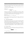
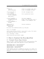
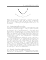
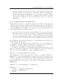
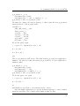
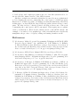
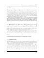
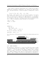
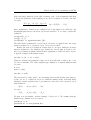
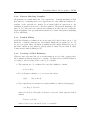
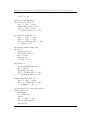
Programming Methodologies in GCLA
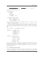
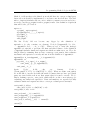
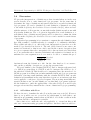
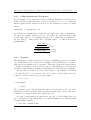
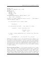
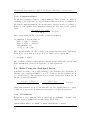
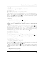
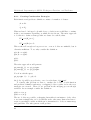
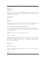
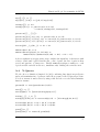
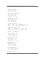
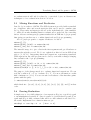
G
H
E
F
C
B
D
A
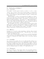
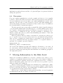
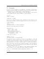
Figure 1: Proof search space for a query S A. A is the query we pose to the
system. The desired procedural behavior is the path leading to G marked in the
figure, however the strategy S instead takes the path via F to H. We localize
the choice-point to C and change the procedural part so that the edge C − E is
chosen instead.
3.1.2
Constructing the Procedural Part
Now, the idea in the minimal stepwise refinement method, is that given a definition D and a set of intended queries Q, we do as little as possible to construct the
procedural part P, that is we try to find strategies S1 , . . . , Sn among the general
strategies given by the system, such that Si Qi , with the intended procedural
behavior for each of the intended queries. If such strategies exist then we are
finished, and constructing the procedural part was trivial indeed. In most cases
however there will be some queries for which we cannot find a predefined strategy which behaves correctly, they all give redundant answers or wrong answers
or even no answers at all.
When there is no default strategy which gives the desired procedural behavior,
we choose the predefined strategy that seems most appropriate and try to alter
the set of proofs it represents so that it will give the desired procedural behavior.
To do this we use the tracer and the statistical package of the GCLA system to
localize the point in the search space of a proof of the query which causes the
faulty behavior. Once we have found the reason behind the faulty behavior we
can remove the error by changing the definition of the procedural part. We then
try all our queries again and repeat the procedure of searching for and correcting
errors of the procedural part until we achieve proper procedural behavior for all
the intended queries. The method is illustrated in Fig. 1.
3.1.3
Example: Disease Expert System Revisited
We try to use the disease program with some standard strategies. For example,
in the query below, the correct answers are X = pneumonia and, on backtracking,
9
Definitional Programming in GCLA: Techniques, Functions, and Predicates
X = plague. The true answers mean that there exists a proof of the query, but
it gives no binding of the variable X.
First we try the strategy arl/0:
| ?- arl \\- (disease(X) \- symptom(high_temp)).
X = pneumonia ? ;
true ? ;
true ? ;
true ? ;
X = plague ? ;
After this we get eight more true answers. Then we try the strategy lra/0:
| ?- lra \\- (disease(X) \- symptom(high_temp)).
This query gives eight true answers before giving the answer pneumonia the
ninth time, then three more true answers and finally the answer plague. We see
that even though it is the case that both arl/0 and lra/0 include proofs of the
query giving the answers in which we are interested, they also include many more
proofs of the query. We therefore try to restrict the set of proofs represented by
the strategy arl/0 in order to remove the undesired answers.
The most typical sources of faulty behavior are that the d_right/2, d_left/3
and axiom/3 rules are applicable in situations where we would rather see they
were not. An example of what can happen is that if, somewhere in the derivation
tree, there is a sequent of the form p\-X, where p is not defined, and the inference
rule d_left/3 is tried and found applicable, we get the new goal false\-X, which
holds since anything can be shown from a false assumption, if we use a strategy
such as arl/0 or lra/0 that contains the false_left/1 rule.
By using the tracer we find that this is what happens in our disease example,
where d_left/3 is tried on the undefined atom disease/1. To get the desired
procedural behavior there are at least two things we could do:
• We could delete the inference rule false_left/1 from our global arl/0
strategy, but then we would never be able to draw a conclusion from a false
assumption.
• We could restrict the d_left/3 rule so that it would not be applicable to
the atom disease/1.
Restricting the d_left/3 rule is very simple and could be made like this:
10
Programming Methodologies in GCLA
d_left(T,I,PT) <=
d_left_applicable(T),
definiens(T,Dp,N),
(PT -> (I@[Dp|R] \- C))
-> (I@[T|R] \- C).
d_left_applicable(T):atom(T),
not(functor(T,disease,1)).
% standard restriction on T
% application specific.
Here we have introduced the proviso d_left_applicable/1 to describe when
d_left/3 is applicable. Apart from the standard restriction that d_left/3 only
applies to atoms we have added the extra restriction that the atom must not be
disease/1.
Now, we try our query again, and this time we get the desired answers and
no others:
| ?- arl \\- (disease(X) \- symptom(high_temp)).
X = pneumonia ? ;
X = plague ? ;
no
With this restriction on the d_left/3 rule the arl/0 strategy correctly handles
all the queries in Sect. 3.1.
3.1.4
Further Refining
One very simple optimization is to use the statistical package of GCLA and
remove any inference rules that are never used from the procedural part.
Sometimes there is a need to introduce new inference rules, for example to
handle numbers in an efficient way. We can then associate an inference rule with
each operation and use this directly to show that something holds. Such new
inference rules could then be placed in one of the strategies user_add_right/2 or
user_add_left/2 which are part of the standard strategies right/1 and left/1.
3.2
Method 2: Splitting the Condition Universe
With the method in the previous section we started to build the procedural part
without paying any particular attention to what the definition and the set of
intended queries looked like. If we study the structure of the definition, and of
the data handled by the program, it is possible to use the knowledge we gain to be
able to construct the procedural part in a more well-structured and goal-oriented
way.
11
Definitional Programming in GCLA: Techniques, Functions, and Predicates
The basic idea in this section is that given a definition D and a set of intended
queries Q, it is possible to divide the universe of all object-level conditions into a
number of classes, where every member of each class is treated uniformly by the
procedural part. Examples of such classes could be the set of all defined atoms,
the set of all terms which could be evaluated further, the set of all canonical
terms, the set of all object level variables etc.
In order to construct the procedural part of a given definition, we first identify
the different classes of conditions used in the definition and in the queries, and
then go on to write the rule definition in such a way that each rule or strategy
becomes applicable to the correct class or classes of conditions. The resulting
rule definition typically consists of some subset of the predefined inference rules
and strategies, extended with a number of provisos which identify the different
classes and decide the applicability of each rule or strategy.
Of course the described method can only be used if it is possible to divide the
object-level condition universe in some suitable set of classes; for some applications this will be very difficult or even impossible to do.
3.3
A Typical Split
The most typical split of the universe of object-level conditions is into one set to
which the d_right/2 and d_left/3 rules but not the axiom/3 rule apply, and
another set to which the axiom/3 rule but not the d_right/2 or d_left/3 rules
apply. To handle this, and many other similar situations easily, we change the
definition of these rules:
d_right(C,PT) <=
d_right_applicable(C),
clause(C,B),
(PT -> (A \- B))
-> (A \- C).
d_left(T,I,PT) <=
d_left_applicable(T),
definiens(T,Dp,N),
(PT -> (I@[Dp|R] \- C))
-> (I@[T|R] \- C).
axiom(T,C,I) <=
axiom_applicable(T),
axiom_applicable(C),
unify(C,T)
-> (I@[T|_] \- C).
12
Programming Methodologies in GCLA
All we have to do now is alter the provisos used in the rules above according to
our split of the universe to get different procedural behaviors. With the proviso
definitions
d_right_applicable(C) :- atom(C).
d_left_applicable(T) :- atom(T).
axiom_applicable(T) :- term(T).
we get exactly the same behavior as with the predefined rules.
3.3.1
Example 1: The Disease Example Revisited
The disease example is an example of an application where we can use the typical
split described above. We know that the d_right/2 and the d_left/3 rules
should only be applicable to the atom symptom/1, so we define the provisos
d_right_applicable/1 and d_left_applicable/1 by:
d_right_applicable(C) :- functor(C,symptom,1).
d_left_applicable(T) :- functor(T,symptom,1).
We also know that the axiom/3 rule should only be applicable to the atom
disease/1, so axiom_applicable/1 thus becomes:
axiom_applicable(T) :- functor(T,disease,1).
3.3.2
Example 2: Functional Programming
One often occurring situation, for example in functional programming, is that
we can split the universe of all object level terms into the two classes of all fully
evaluated expressions and variables and all other terms respectively.
For example, if the class of fully evaluated expressions consists of all numbers
and all lists, it can be defined with the proviso canon/1:
canon(X) :- number(X).
canon([]).
canon(X) :- functor(X,’.’,2).
To get the desired procedural behavior we restrict the axiom/3 rule to operate
on the class defined by the above proviso and the set of all variables, and the
d_right/2 and d_left/3 rules to operate on any other terms, thus:
d_right_applicable(T):atom(T),not(canon(T)).
d_left_applicable(T):-
% noncanonical atom
13
Definitional Programming in GCLA: Techniques, Functions, and Predicates
atom(T),not(canon(T)).
% noncanonical atom
axiom_applicable(T) :- var(T).
axiom_applicable(T) :- nonvar(T),canon(T).
Here we use not/1 to indicate that if we cannot prove that a term belongs to the
class of canonical terms then it belongs to the class of all other terms.
3.4
Method 3: Local Strategies
Both of the previous methods are somehow based on the idea that we should
start with a general search strategy, among the inference rules at hand, and
restrict or augment the set of proofs it represents in order to get the desired
procedural behavior from a given definition and its associated set of intended
queries. However, we could just as well do it the other way around and study
the definition and the set of intended queries and construct a procedural part,
that gives us exactly the procedural interpretation we want right from the start,
instead of performing a tedious procedure of repeatedly cutting away (or adding)
branches of the proof search space of some general strategy. In this section we
will show how this can easily be done for many applications. Any examples will
use the standard rules, but the method as such works equivalently with any set
of rules.
3.4.1
Collecting Knowledge
When constructing the procedural part we try to collect and use as much knowledge as possible about the definition, the set of intended queries, of how the
GCLA system works etc. Among the things we need to take into account in
order to construct the procedural part properly are:
• We need to have a good idea of how the GCLA system tries to construct
the proof of a query.
• We must have a thorough understanding of the interpretation of the predefined rules and strategies, and of any new rules or strategies we write.
• We must decide exactly what the set of intended queries is. For example,
in the disease example this set is as described in Sect. 3.1.
• We must study the structure of the definition in order to find out how each
defined atom should be used procedurally in the queries. This involves
among other things considering whether it will be used with the d_left/3
or the d_right/2 rule or both. For example, in the disease example we
know that both the d_left/3 and the d_right/2 rule should be applicable
to the atom symptom/1, but that neither of them should be applicable to
14
Programming Methodologies in GCLA
the atom disease/1. We also use knowledge of the structure of the possible
sequents occurring in a derivation, to decide if we will need a mechanism for
searching among several assumptions or to decide where to use the axiom/3
rule etc. For example, in the disease example we know that the axiom/3
rule should be applicable to the atom disease/1, but not to the atom
symptom/1.
3.4.2
Constructing the Procedural Part
Assume that we have a set of condition constructors, C, with a corresponding set
of inference rules, R. Given a definition D which defines a set of atoms DA, a set
of intended queries Q and possibly another set U A of undefined atoms which can
occur as assumptions in a sequent, we do the following to construct strategies for
each element in the set of intended queries:
• Associate with each atom in the sets DA and U A, a distinct procedural part
that assures that the atoms are used the way we want in all situations where
they can occur in a derivation tree. The procedural part associated with
an atom is built using the elements of R, d_right/2, d_left/3, axiom/3,
strategies associated with other atoms and any new inference rules needed.
We can then use the strategies defined above to build higher-level strategies for
all the intended queries in Q.
For example, in the disease example C is the set {‘;’/2,‘,’/2}, R is the set
{o_right/3,o_left/4,v_right/3,v_left/3}, D and Q are as given in Sect.
3.1, DA is the set {symptom/1} and U A is the set {disease/1}.
According to the method we should first write distinct strategies for each
member of DA, that is symptom/1. The atom symptom/1 can occur on the right
side of the object level sequent so we write a strategy for this case:
symptom_r <= d_right(symptom(_),disease).
When symptom/1 occurs on the right side we want to look up the definition of
symptom/1 so we use the d_right/2 rule, giving a new object level sequent of the
form A \- disease(X), and we therefore continue with the strategy disease/0.
Now, symptom/1 is also used on the left side and since we can not use
symptom_r/0 to the left, we have to introduce a new strategy for this case,
symptom_l/0:
symptom_l <= d_left(symptom(_),_,symptom_l2).
symptom_l2 <=
o_left(_,_,symptom_l2,symptom_l2),
o_right(_,_,symptom_l2),
disease.
15
Definitional Programming in GCLA: Techniques, Functions, and Predicates
When symptom/1 occurs on the left side we want to calculate the
definiens of symptom/1 so we can use the d_left/3 rule, giving a
new object level sequent of the form (disease(Y1 );...;disease(Yn )) \(disease(X1 );. . . ;disease(Xk )). In this case we continue with the strategy
symptom_l2/0, which handles sequents of this form. The strategy symptom_l2/0
uses the strategy disease/0 to handle the individual disease/1 atoms.
We now define the disease/0 strategy:
disease <= axiom(disease(_),_,_).
Finally we use the strategies defined above to construct strategies for all the
intended queries. The first kind of query is of the form disease(D) \symptom(X1 ),... ,symptom(Xn ). These queries can be handled by the following strategy:
d1 <= v_right(_,symptom_r,d1),symptom_r.
The second kind of query is of the form symptom(S) \(disease(X1 );...;disease(Xn )). These queries are handled by the strategy
d2/0:
d2 <= symptom_l.
What we actually do with this method is to assign a local procedural interpretation
to each atom in the sets DA and U A. This local procedural interpretation is
specialized to handle the particular atom correctly in every sequent in which
it occurs. The important thing is that the procedural part associated with an
atom ensures that we will get the correct procedural behavior if we use it in the
intended way, no matter what rules or strategies we write to handle other atoms
of the definition. Since each atom has its own local procedural interpretation, we
can use different programming methodologies and different sorts of procedural
interpretations for the particular atom in different parts of the program.
In practice this means that for each atom in DA and U A we write one or more
strategies which are constructed to correctly handle the particular atom. One way
to do this is to define the basic procedural behavior of each atom, by which we
mean that given an atom, say p/1, we define the basic procedural behavior of p/1
(in this application) as how we want it to behave in a query where it is directly
applicable to one of the inference rules d_right/2, d_left/3 or axiom/3, that is
queries of the form A \-p(X) or A1 ,...,p(X),...,An \- C.
Since the basic strategy of an atom can use the basic strategy of any other
defined atom if needed, and since strategies of more complex queries can use
any combination of strategies, we will get a hierarchy of strategies, where each
member has a well-defined procedural behavior. In the bottom of this hierarchy
we find the strategies that do not use any other strategies, only rules, and in the
top we have the strategies used by a user to pose queries to the system.
16
Programming Methodologies in GCLA
3.4.3
Example
In the disease example we constructed the procedural part bottom-up. In practice
it is often better to work top-down from the set of intended queries, since most
of the time we do not know exactly what strategies are needed beforehand.
This means that we start with an intended query, say A1 ,...,An \- p(X),
constructing a top level strategy for this assuming that we already have all substrategies we need, and then go on to construct these sub-strategies so that they
behave as we have assumed them to do.
The following small example could be used to illustrate the methodology:
classify(X) <=
wheels(W),engine(E),(class(wheels(W),engine(E)) -> X).
class(wheels(4),engine(yes)) <= car.
class(wheels(2),engine(yes)) <= motorbike.
class(wheels(2),engine(no)) <= bike.
The only intended query is A1 ,...,An \- classify(X), where we use the lefthand side to give observations and try to conclude a class from them, for example:
| ?- classify \\- (engine(yes),wheels(2) \- classify(X)).
X = motorbike ? ;
no
We start from the top and assuming that we have suitable strategies for the queries A1 ,...,A \- wheels(X), A1 ,...,An \- engine(X)
and A1 ,...,class(X),...,An \- C, we construct the top level strategy
classify/0:
%classify \\- (A \- classify(X))
classify <=
d_right(_,v_rights(_,_,[wheels,engine,a_right(_,class)])).
where v_rights/3 is a rule that is used as an abbreviation for several consecutive
applications of the v_right/3 rule. All we have left to do now is to construct the
sub-strategies. The strategies engine/0 and wheels/0 are identical; engine/1
and wheels/1 are given as observations in the left-hand side, so we use the
axiom/3 rule to communicate with the right side, giving the basic strategies:
%engine \\- (A1,,engine(X),,An \- Conc)
engine <= axiom(engine(_),_,_).
%wheels \\- (A1,,wheels(X),,An \- Conc)
wheels <= axiom(wheels(_),_,_).
17
Definitional Programming in GCLA: Techniques, Functions, and Predicates
Finally class/0 is a function from the observed properties to a class, and the
rule definition we want is:
%class \\- (A1,,class(X,Y),,An \- Conc)
class <= d_left(class(_,_),I,axiom(_,_,I)).
Of course we do not always have to be so specific when we construct the strategies
and sub-strategies if we find it unnecessary.
4
A Larger Example: Quicksort
In this section we will use the three methods described above to develop some
sample procedural parts to a given definition and an intended set of queries. Of
course, due to lack of space it is not possible to give a realistic example, but we
think that the basic ideas will shine through.
The given definition is a quicksort program, earlier described in [1] and [2],
which contains both functions and relational programming as well as the use of
new condition constructors.
4.1
The Definition
Here is the definition of the quicksort program:
qsort([]) <= [].
qsort([F|R]) <=
pi L \ (pi G \ (split(F,R,L,G) ->
append(qsort(L),cons(F,qsort(G))))).
split(_,[],[],[]).
split(E,[F|R],[F|Z],X) <= E >= F,split(E,R,Z,X).
split(E,[F|R],Z,[F|X]) <= E < F,split(E,R,Z,X).
append([],F) <= F.
append([F|R],X) <= cons(F,append(R,X)).
append(X,Y)#{X \= [_|_],X \= []} <=
pi Z\ ((X -> Z) -> append(Z,Y)).
cons(X,Y) <= pi Z \ (pi W \ ((X -> Z), (Y -> W) -> [Z|W])).
In the definition above qsort/1, append/2 and cons/2 are functions, while
split/4 is a relation. There are also two new condition constructors: ‘>=’/2
and ‘<’/2.
We will only consider one intended query
qsort(X) \- Y .
18
Programming Methodologies in GCLA
where X is a list of numbers and Y is a variable to be instantiated to a sorted
permutation of X.
4.2
Method 1
We first try the predefined strategy gcla/0 (the same as arl/0):
| ?- gcla \\- (qsort([4,1,2]) \- X).
X = qsort([4,1,2]) ?
yes
By using the debugging tools, we find out that the fault is that the axiom/3 rule
is applicable to qsort/1. We therefore construct a new strategy, q_axiom/3, that
is not applicable to qsort/1:
q_axiom(T,C,I) <=
not(functor(T,qsort,1)) -> (I@[T|_] \- C).
q_axiom(T,C,I) <= axiom(T,C,I).
We must also change the arl/0 strategy so that it uses q_axiom/3 instead of
axiom/3:
arl <= q_axiom(_,_,_),right(arl),left(arl).
Then we try the query again:
| ?- gcla \\- (qsort([4,1,2]) \- X).
no
This time the fault is that we have no rules for the new condition constructors
‘>=’/2 and ‘<’/2. So we write two new rules, ge_right/1 and lt_right/1, which
we add to the predefined strategy user_add_right/2:
ge_right(X >= Y) <=
number(X),
number(Y),
X >= Y
-> (A \- X >= Y).
lt_right(X < Y) <=
number(X),
number(Y),
X < Y
-> (A \- X < Y).
19
Definitional Programming in GCLA: Techniques, Functions, and Predicates
Here number/1 is a predefined proviso.
We try the query again:
| ?- gcla \\- (qsort([4,1,2]) \- X).
X = append(qsort([1,2]),cons(4,qsort([]))) ?
yes
We find out that the fault is that the q_axiom/3 strategy should not be applicable
to append/2. We therefore refine the strategy q_axiom/3 so it is not applicable
to append/2 either:
q_axiom(T,C,I) <=
not(functor(T,qsort,1),
not(functor(T,append,2) -> (I@[T|_] \- C).
q_axiom(T,C,I) <= axiom(T,C,I).
We try the query again:
| ?- gcla \\- (qsort([4,1,2]) \- X).
...
This time we get no answer at all. The problem is that the q_axiom/3 strategy
is applicable to cons/2. So we refine q_axiom/3 once again:
q_axiom(T,C,I) <=
not(functor(T,qsort,1)),
not(functor(T,append,2)),
not(functor(T,cons,2)) -> (I@[T|_] \- C).
q_axiom(T,C,I) <= axiom(T,C,I).
We try the query again:
| ?- gcla \\- (qsort([4,1,2]) \- X).
X = [1,2,4] ? ;
true ?
yes
The first answer is obviously correct but the second is not. Using the debugging
facilities once again, we find out that the problem is that the d_left/3 rule
is applicable to lists, so we construct a new strategy, q_d_left/3, that is not
applicable to lists:
20
Programming Methodologies in GCLA
q_d_left(T,I,_) <=
not(functor(T,[],0)),
not(functor(T,’.’,2)) -> (I@[T|_] \- _).
q_d_left(T,I,PT) <= d_left(T,I,PT).
We must also change the left/1 strategy, so that it uses the new q_d_left/3
strategy instead of the d_left/3 rule:
left(PT) <=
user_add_left(_,_,PT),
false_left(_),
v_left(_,_,PT),
a_left(_,_,PT,PT),
o_left(_,_,PT,PT),
q_d_left(_,_,PT),
pi_left(_,_,PT).
We try the query again:
| ?- gcla \\- (qsort([4,1,2]) \- X).
X = [1,2,4] ? ;
X = [1,2,_A] ?
yes
The second answer is still wrong. The fault is that q_d_left/3 is applicable to
numbers. We therefore refine the strategy q_d_left/3 so it is not applicable to
numbers either:
q_d_left(T,I,_) <=
not(functor(T,[],0)),
not(functor(T,’.’,2)),
not(number(T)) -> (I@[T|_] \- _).
q_d_left(T,I,PT) <= d_left(T,I,PT).
We try the query once again:
| ?- gcla \\- (qsort([4,1,2]) \- X).
X = [1,2,4] ? ;
no
And finally we get all the correct answers and no others.
One last simple refinement is to use the statistical package to remove unused
strategies and rules. The complete rule definition thus becomes:
21
Definitional Programming in GCLA: Techniques, Functions, and Predicates
arl <= q_axiom(_,_,_),right(arl),left(arl).
left(PT) <=
a_left(_,_,PT,PT),
q_d_left(_,_,PT),
pi_left(_,_,PT).
q_d_left(T,I,_) <=
not(functor(T,[],0)),
not(functor(T,’.’,2)),
not(number(T)) -> (I@[T|_] \- _).
q_d_left(T,I,PT) <= d_left(T,I,PT).
user_add_right(C,_) <= ge_right(C),lt_right(C).
q_axiom(T,C,I) <=
not(functor(T,qsort,1)),
not(functor(T,append,2)),
not(functor(T,cons,2)) -> (I@[T|_] \- C).
q_axiom(T,C,I) <= axiom(T,C,I).
ge_right(X >= Y) <=
number(X),
number(Y),
X >= Y
-> (A \- X >= Y).
lt_right(X < Y) <=
number(X),
number(Y),
X < Y
-> (A \- X < Y).
constructor(>=,2).
constructor(<,2).
4.3
Method 2
First we use our knowledge about the general structure of GCLA programs.
Among the default rules all but d_left/3, d_right/2 and axiom/3 are applicable to condition constructors only. One possible split is therefore the set of all
constructors and the set of all conditions that are not constructors, that is terms:
cond_constr(E) :- functor(E,F,A),constructor(F,A).
22
Programming Methodologies in GCLA
terms(E) :- term(E).
Now, all terms can in turn be divided into variables and terms that are not
variables, that is atoms. We therefore split the terms/1 class into the set of
variables and the set of atoms:
vars(E) :- var(E).
atoms(E) :- atom(E).
The atoms can be divided further into all defined atoms and all undefined atoms.
In this application we only want to apply the d_left/3 and d_right/2 rules to
defined atoms. We also know that the only undefined atoms are numbers and
lists, that is the data handled by the program, so one natural split could be the
set of all defined atoms and the set of all undefined atoms:
def_atoms(E) :functor(E,F,A),d_atoms(DA),member(F/A,DA).
undef_atoms(E) :- number(E).
undef_atoms(E) :- functor(E,[],0);functor(E,’.’,2).
In this application the defined atoms are qsort/1, split/4, append/2 and
cons/2:
d_atoms([qsort/1,split/4,append/2,cons/2]).
Now we use our knowledge about the application. Our intention is to use qsort/1,
append/2 and cons/2 as functions and split/4 as a predicate. In GCLA functions are evaluated on the left side of the object level sequent and predicates are
used on the right. We therefore further divide the class def_atoms/1 into the set
of defined atoms used to the left and the set of defined atoms used to the right:
def_atoms_r(E) :functor(E,F,A),d_atoms_r(DA),member(F/A,DA).
def_atoms_l(E) :functor(E,F,A),d_atoms_l(DA),member(F/A,DA).
d_atoms_r([split/4]).
d_atoms_l([qsort/1,append/2,cons/2]).
We now construct our new q_d_right/2 strategy which restricts the d_right/2
rule to be applicable only to members of the class def_atoms_r/1, that is all
defined atoms used to the right:
23
Definitional Programming in GCLA: Techniques, Functions, and Predicates
q_d_rigth(C,PT) <=
def_atoms_r(C) -> (_ \- C).
q_d_right(C,PT) <= d_right(C,PT).
The d_left/3 rule is restricted similarly by the q_d_left/3 strategy.
Since the axiom/3 rule is used to unify the result of a function application
with the right hand side, we only want it to be applicable to numbers, lists and
variables, that is to the members of the classes undef_atoms/1 and vars/1. We
therefore create a new class, data/1, which is the union of these two classes:
data(E) :- vars(E).
data(E) :- undef_atoms(E).
And the new q_axiom/3 strategy thus becomes:
q_axiom(T,C,I) <=
data(T),
data(C) -> (I@[T|_] \- C).
q_axiom(T,C,I) <= axiom(T,C,I).
What is left are the strategies for the first class, cond_constr/1. We use the
default strategy c_right/2 to construct our new q_c_right/2 strategy:
q_c_right(C,PT) <=
cond_constr(C) -> (_ \- C).
q_c_right(C,PT) <= c_right(C,PT),ge_right(C),lt_right(C).
Similarly, q_c_left/3 is defined by:
q_c_left(T,I,PT) <=
cond_constr(T) -> (I@[T|_] \- _).
q_c_left(T,I,PT) <= c_left(T,I,PT).
Finally we must have a top-strategy, qsort/0:
qsort <=
q_c_left(_,_,qsort),
q_d_left(_,_,qsort),
q_c_right(_,qsort),
q_d_right(_,qsort),
q_axiom(_,_,_).
Thus, the complete rule definition (where we have removed redundant classes)
becomes:
24
Programming Methodologies in GCLA
% Class definitions
cond_constr(E) :- functor(E,F,A),constructor(F,A).
def_atoms_r(E) :- functor(E,F,A),d_atoms_r(DA),member(F/A,DA).
def_atoms_l(E) :- functor(E,F,A),d_atoms_l(DA),member(F/A,DA).
undef_atoms(E) :- number(E).
undef_atoms(E) :- functor(E,[],0);functor(E,’.’,2).
data(E) :- var(E).
data(E) :- undef_atoms(E).
d_atoms_r([split/4]).
d_atoms_l([qsort/1,append/2,cons/2]).
% Strategy definitions
qsort <=
q_c_left(_,_,qsort),
q_d_left(_,_,qsort),
q_c_right(_,qsort),
q_d_right(_,qsort),
q_axiom(_,_,_).
q_c_right(C,PT) <=
cond_constr(C) -> (_ \- C).
q_c_right(C,PT) <= c_right(C,PT),ge_right(C),lt_right(C).
q_c_left(T,I,PT) <=
cond_constr(T) -> (I@[T|_] \- _).
q_c_left(T,I,PT) <= c_left(T,I,PT).
q_axiom(T,C,I) <=
data(T),
data(C) -> (I@[T|_] \- C).
q_axiom(T,C,I) <= axiom(T,C,I).
q_d_rigth(C,PT) <=
def_atoms_r(C) -> (_ \- C).
q_d_right(C,PT) <= d_right(C,PT).
ge_right(X >= Y) <=
number(X),
25
Definitional Programming in GCLA: Techniques, Functions, and Predicates
number(Y),
X >= Y
-> (A \- X >= Y).
lt_right(X < Y) <=
number(X),
number(Y),
X < Y
-> (A \- X < Y).
q_d_left(T,I,PT) <=
def_atoms_l(T) -> (I@[T|_] \- _).
q_d_left(T,I,PT) <= d_left(T,I,PT).
constructor(>=,2).
constructor(<,2).
4.4
Method 3
We will construct the procedural part working top-down from the intended query.
As the set of rules R, we use the predefined rules augmented with the rules
ge_right/1 and lt_right/1 used above. We will use a list, U ndef , to hold all
meta level sequents that we have assumed we have procedural parts for but not
yet defined. When this list is empty the construction of the procedural part is
finished.
When we start U ndef contains one element, the intended query,
U ndef = [(qsort(I) \\- (qsort(L) \- Sorted))]. We then define the
strategy qsort/1:
qsort(I) <= d_left(qsort(_),I,qsort(_,I)).
qsort(T,I) <=
(I@[T|R] \- C).
qsort(T,I) <=
qsort2(T,I).
qsort2([],I) <=
axiom([],_,I).
qsort2((pi _ \ _),I) <=
pi_left(_,I,pi_left(_,I,a_left(_,I,split,append(I)))).
Now
U ndef
contains
two
elements,
U ndef =
[(split \\- (A \split(F ,R,G,L))),
(append(I) \\- (A 1 ,...,
append(L1 ,L2 ) ,...,An \- L))]. The next strategy to define is split/0.
26
Programming Methodologies in GCLA
Method 3 tells us that each defined atom should have its own procedural part,
but not how it should be implemented, so we have some freedom here. The definition of split/4 includes the two new condition constructors >=/2 and </2 so
we need to use the ge_right/1 and lt_right/1 rules. One definition of split/0
that will do the job for us is:
split <=
v_right(_,split,split),
d_right(split(_,_,_,_),split),
gt_right(_),
lt_right(_),
true_right.
The list U ndef did not become any bigger by the definition of
split/0 so it only contains one element, U ndef = [(append(I) \\- (A 1 ,
...,append(L1 ,L2 ),...,An \- L))]. When we try to write the strategy
append/1 we run into a problem; the first and third clauses of the definition
of append/2 includes functional expressions which are unknown to us. We solve
this problem by assuming that we have a strategy, eval_fun/3, that evaluates
any functional expression correctly and use it in the definition of append2/1:
append(I)<= d_left(append(_,_),I,append2(I)).
append2(I) <=
pi_left(_,I,a_left(_,I,a_right(_,
eval_fun(_,[],_)),append(I))),
eval_fun(_,I,_).
Again
U ndef
holds
only
one
element,
U ndef =
[(eval_fun(T ,I,P T ) \\- (I@[T |R] \- C))]. When we define eval_fun/3
we would like to use the fact that the method ensures that we have procedural
parts associated with each atom, that assure that it is used correctly. We do
this by defining a proviso, case_of/3, which will choose the correct strategy for
evaluating any functional expression. Lists and numbers are regarded as fully
evaluated functional expressions whose correct procedural part is axiom/3:
eval_fun(T,I,PT)<=
case_of(T,I,PT) -> (I@[T|R] \- C).
eval_fun(T,I,PT) <= PT.
case_of(cons(_,_),I,cons(I)).
case_of(append(_,_),I,append(I)).
case_of(qsort(_),I,qsort(I)).
case_of(T,I,axiom(_,_,I)) :- canon(T).
canon([]).
27
Definitional Programming in GCLA: Techniques, Functions, and Predicates
canon(X):- functor(X,.,2).
canon(X):- number(X).
In the proviso case_of/3 we introduced a new strategy cons/1, so U ndef is still
not empty, U ndef = [(cons(I) \- (A1 ,...,cons(H,T ),...,An \- L))].
When we define cons/1 we again encounter unknown functional expressions, to
be evaluated, and use the eval_fun/3 strategy:
cons(I) <=
d_left(cons(_,_),I,pi_left(_,I,pi_left(_,I,a_left(_,I,
v_right(_,a_right(_,eval_fun(_,[],_)),
a_right(_,eval_fun(_,[],_))),
axiom(_,_,I))))).
Now U ndef is empty, so we are finished. In the rule definition below we used a
more efficient split/0 strategy than the one defined above:
% top-level strategy
% qsort \\- (I@[qsort(List)|R] \- SortedList).
qsort <= qsort(_).
qsort(I) <= d_left(qsort(_),I,qsort(_,I)).
qsort(T,I) <=
(I@[T|R] \- C).
qsort(T,I) <=
qsort2(T,I).
qsort2([],I) <=
axiom([],_,I).
qsort2((pi _ \ _),I) <=
pi_left(_,I,pi_left(_,I,a_left(_,I,split,append(I)))).
% split \\- (A \- split(A,B,C,D)).
split <= d_right(split(_,_,_,_),split(_)).
split(C) <=
(_ \- C).
split(C) <=
split2(C).
split2(true) <=
true_right.
split2((_ >= _,_)) <=
v_right(_,ge_right(_),split).
split2((_ < _,_)) <=
28
Programming Methodologies in GCLA
v_right(_,lt_right(_),split).
% append(I) \\- (I@[append(L1,L2)|R] \- L).
append(I) <= d_left(append(_,_),I,append2(I)).
append2(I) <=
pi_left(_,I,a_left(_,I,a_right(_,
eval_fun(_,[],_)),append(I))),
eval_fun(_,I,_).
% only tried if the strategy on
% the line above fails
% cons \\- (I@[cons(Hd,Tl)|R] \- L).
cons(I) <=
d_left(cons(_,_),I,pi_left(_,I,pi_left(_,I,
a_left(_,I,v_right(_,a_right(_,eval_fun(_,[],_)),
a_right(_,eval_fun(_,[],_))),
axiom(_,_,I))))).
% eval_fun(T,I,PT) \\- (I@[T|R] \- C)
eval_fun(T,I,PT)<=
case_of(T,I,PT) -> (I@[T|R] \- C).
eval_fun(T,I,PT) <= PT.
case_of(cons(_,_),I,cons(I)).
case_of(append(_,_),I,append(I)).
case_of(qsort(_),I,qsort(I)).
case_of(T,I,axiom(_,_,I)) :- canon(T).
canon([]).
canon(X):- functor(X,’.’,2).
canon(X):- number(X).
ge_right(X >= Y) <=
number(X),
number(Y),
X >= Y
-> (A \- X >= Y).
lt_right(X < Y) <=
number(X),
number(Y),
X < Y
-> (A \- X < Y).
29
Definitional Programming in GCLA: Techniques, Functions, and Predicates
constructor(>=,2).
constructor(<,2).
5
Discussion
In this section we will evaluate each method according to five criteria on how
good we perceive the resulting programs to be.
The following criteria will be used:
1. Correctness—Naturally, one of the major requirements of a programming
methodology is to ensure a correct result. We will use the correctness
criterion as a measure of how easy it is to construct correct programs,
that is to what extent the method ensures a correct result and how easy
it is to be convinced that the program is correct. A program is correct if
it has the intended behavior, that is for each of the intended queries we
receive all correct answers and no others. Since we are only interested in
the construction of the procedural part, that is the rule definition, we can
assume that the definition is intuitively correct.
2. Efficiency—We also want to compare the efficiency of the resulting programs. The term efficiency involves not only such things as execution time
and the size of the programs, but also the overall cost of developing programs using the method in question.
3. Readability—We will use the readability criterion to measure the extent to
which the particular method ensures that the resulting programs are easy
to read and easy to understand.
4. Maintenance—Maintenance is an important issue when programming-inthe-large. We will use the term maintenance to measure the extent to
which the method in question ensures that the resulting programs are easy
to maintain, that is how much extra work is implied by a change to the
definition or the rule definition.
5. Reusability—Another important issue when programming-in-the-large is the
notion of reusability. By this we mean to what extent the resulting programs can be used in a large number of different queries and to what extent
the specific method supports modular programming, that is the possibility
of saving programs or parts of programs in libraries for later usage in other
programs, if different parts of the programs can easily be replaced by more
efficient ones etc. For the purpose of the discussion of this criterion we
define a module to mean a definition together with a corresponding rule
definition with a well-defined interface of queries.
30
Programming Methodologies in GCLA
5.1
5.1.1
Evaluation of Method 1
Correctness
If the number of possible queries is small we are likely to be able to convince
ourselves of the correctness of the program, but if the number of possible queries
is so large that there is no way we can test every query, then it could be very
hard to decide whether the current rule definition is capable of deriving all the
correct answers or not.
This uncertainty goes back to the fact that the rule definition is a result of
a trial and error-process; we start out testing a very general strategy and only
if this strategy fails in giving us all the correct answers, or if it gives us wrong
answers, we refine the strategy to a less general one to remedy this misbehavior.
Then we start testing this refined strategy and so on. The problem is that we
cannot be sure we have tested all possible cases, and as we all know testing can
only be used to show the presence of faults, not their absence.
The uncertainty is also due to the fact that the program as a whole is the
result of stepwise refinement, that is successive updates to the definition and the
rule definition, and when we use Method 1 to construct programs we have very
little control over all consequences that a change to the definition or the rule
definition brings with it, especially when the programs are large.
5.1.2
Efficiency
Sometimes we do not need to write any strategies or inference rules at all, the
default strategies and the default rules will do. This makes many of the resulting
programs very manageable in size.
Due to the fact that the method by itself removes very little indeterminism
in the search space, the resulting programs are often slow however. We can of
course keep on refining the rule definition until we have a version that is efficient
enough.
5.1.3
Readability
On one hand, since programs often are very small and make extensive use of
default strategies and rules, they are very comprehensible. On the other hand,
if you keep on refining long enough so that the final rule definition consists of
many highly specialized strategies and rules, all very much alike in form, with
conditions and exceptions on their respective applicability in the form of provisos,
then the resulting programs are not likely to be comprehensible at all.
5.1.4
Maintenance
Since the rule definition to a large extent consists of very general rules and strategies, a change or addition to the definition does not necessarily imply a corre31
Definitional Programming in GCLA: Techniques, Functions, and Predicates
sponding change or addition to the rule definition.
The first problem then is to find out if we must change the rule definition as
well. As long as the programs are small and simple this is not much of a problem,
but for larger and more complex programs this task can be very time-consuming
and tedious.
If we find out that the rule definition indeed has to be changed, then another problem arises. Method 1 is based on the principle that we use as general
strategies and inference rules as possible. This means that many strategies and
rules are applicable to many different derivation steps in possibly many different
queries. Therefore, when we change the rule definition we have to make sure that
this change does not have any other effects than those intended, as for example
redundant, missing or wrong answers and infinite loops. Once again, if the programs are small and simple this is not a serious problem, but for larger and more
complex programs this is a very time-consuming and non-trivial task.
The fact is that for large programs the work needed to overcome these two
problems is so time-consuming that it is seldom carried out in practice. It is due
to this fact that it is so hard to be convinced of the correctness of large complex
programs, developed using Method 1.
5.1.5
Reusability
Due to the very general rule definition, programs constructed with Method 1
can often be used in a large number of different queries. However, by the same
reason it can be very hard to reuse programs or parts of programs developed using
Method 1 in other programs developed using the same method, since it’s likely
that their respective rule definitions (which are very general) will get into conflict
with each other. But, as we will see in Sect. 5.3, if we want to reuse programs
or parts of programs constructed with Method 1 in programs constructed with
Method 3, we will not have this problem. Thus, the reusability of programs
developed using Method 1 depends on what kind of programs we want to reuse
them in.
5.2
5.2.1
Evaluation of Method 2
Correctness
Programs developed with Method 1 and Method 2 respectively, can be very much
alike in form. The most important difference is that with the former method,
programs are constructed in a rather ad hoc way; the final programs are the result
of a trial and error-process. A program is refined through a series of changes to
the definition and to the rule definition, and the essential thing about this is that
these changes are to a great extent based on the program’s external behavior, not
on any deeper knowledge about the program itself or the data handled by the
program.
32
Programming Methodologies in GCLA
In the latter method, programs are constructed using knowledge about the
classification, the programs themselves and the data handled by the programs.
This knowledge makes it easier to be convinced that the programs are correct.
5.2.2
Efficiency
Compared to programs developed with Method 1, programs constructed using
Method 2 are often somewhat larger. However, when it comes to execution time,
programs developed using Method 2 are generally faster, since much of the indeterminism, which when using Method1 requires a lot of refining to get rid off,
disappears more or less automatically in Method 2, when we make our classification. Thus, we get faster programs for the same amount of work, by using
Method 2 rather than Method 1.
5.2.3
Readability
A program constructed using Method 2 is mostly based on the programmer’s
knowledge about the program and on the knowledge about the objects handled
by the program. Therefore, if we understand the classification we will understand
the program.
The rule definitions of the resulting programs often consist of very few strategies and rules, which make them even easier to understand.
5.2.4
Maintenance
When we have changed the definition we must do the following, to ensure that
the rule definition can be used in the intended queries:
1. For every new object that belongs to an already existing class, we add the
new object as a new member of the class in question. No strategies or rules
have to be changed.
2. For every new object that belongs to a new class, we define the new class
and add the new object as a new member of the newly defined class. We
then have to change all strategies and rules so that they correctly handle
the new class. This work can be very time-consuming.
If the changes only involves objects that are already members of existing classes,
we do not have to do anything.
If we change a strategy or a rule in the rule definition, we only have to make
sure that the new strategy or rule correctly handles all existing classes. Of course,
this work can be very time-consuming.
By introducing well-defined classes of objects we get a better control of the
effects caused by changes to the definition and the rule definition, compared to
what we get using Method 1. Many of the costly controls needed in the latter
33
Definitional Programming in GCLA: Techniques, Functions, and Predicates
method, can in the former method be reduced to less costly controls within a
single class.
5.2.5
Reusability
Due to the very general rule definition, programs developed using Method 2 can
often be used in a large number of different queries. Yet, by the same reasons
as in Method 1, it can be difficult to reuse programs or parts of programs developed using Method 2 in other programs developed using the same method (or
Method 1).
Nevertheless, we can use Method 2 to develop libraries of rule definitions for
certain classes of programs, for example functional and object-oriented programs.
5.3
5.3.1
Evaluation of Method 3
Correctness
The rule definitions of programs constructed using Method 3, consist of a hierarchy of strategies, at the top of which we find the strategies that are used by
the user in the derivations of the queries, and in the bottom of which we find the
strategies and rules that are used in the derivations of the individual atoms.
Since the connection between each atom in the definition and the corresponding part of the rule definition (that is the part that consists of those strategies
and rules that are used in the derivations of this particular atom) is very direct,
it is most of the time very easy to be convinced that the program is correct.
Method 3 also gives, at least some support to modular programming, which
gives us the possibility of using library definitions, with corresponding rule definitions, in our programs. These definitions can often a priori be considered
correct.
5.3.2
Efficiency
One can say that Method 3 is based on the principle: One atom one strategy”.
This makes the rule definitions of the resulting programs very large, in some
cases even as large as the definition itself. When constructing programs using
Method 3, we may therefore get the feeling of “writing the program twice”.
The large rule definitions and all this writing are a severe drawback of
Method 3. However, the writing of the strategies often follows certain patterns,
and most of the work of constructing the rule definition can therefore be carried
out more or less mechanically. The possibility of using library definitions, with
corresponding rule definitions, also reduces this work.
Programs constructed using Method 3 are often very fast. There are two main
reasons for this:
34
Programming Methodologies in GCLA
1. The hierarchical structure of the rule definition implies that in every step
of the derivation of a query, large parts of the search space can be cut away.
2. The method encourages the programmer to write very specialized and efficient strategies for common definitions. In practice, large parts of the
derivation of a query is therefore completely deterministic.
5.3.3
Readability
Programs constructed using Method 3 often have large rule definitions and may
therefore be hard to understand. Still, the “one atom—one strategy”-principle
and the hierarchical structure of the rule definitions make it very easy to find
those strategies and rules that handle a specific part of the definition and vice
versa, especially if we follow the convention of naming the strategies after the
atoms they handle.
The possibility of using common library definitions, with corresponding rule
definitions, also increases the understanding of the programs.
5.3.4
Maintenance
Programs developed using Method 3 are easy to maintain. This is due to the
direct connection between the atoms of the definition and the corresponding part
of the rule definition.
If we change some atoms in the definition, only those strategies corresponding to these atoms might need to be changed, no other strategies have to be
considered.
If we change an already existing strategy in the rule definition, we only have to
make sure that the corresponding atoms in the definition, are handled correctly by
the new strategy. We also do not need to worry about any unwanted side-effects
in the other strategies, caused by this change.
Thus, we see that changes to the definition and the rule definition are local,
we do not have to worry about any global side-effects. Most of the time this is
exactly what we want, but it also implies that it is hard to carry out changes,
where we really do want to have a global effect.
5.3.5
Reusability
Method 3 is the only method that can be said to give any real support to modular
programming. Thanks to the very direct connection between the atoms of the
definition and the corresponding strategies in the rule definition, it is easy to
develop small independent definitions, with corresponding rule definitions, which
can be assembled into larger programs, or be put in libraries of common definitions
for later usage in other programs.
35
Definitional Programming in GCLA: Techniques, Functions, and Predicates
Still, for the same reason, programs developed using Method 3 are less flexible
when it comes to queries, compared to the two previous methods. The rule
definition is often tailored to work with a very small number of different queries.
Of course, we can always write additional strategies and rules that can be used
in a larger number of queries, but this could mean that we have to write a new
version of the entire rule definition.
6
Conclusions
In this paper we have presented three methods of constructing the procedural
part of a GCLA program:minimal stepwise refinement, splitting the condition
universe and local strategies. We have also compared these methods according to
five criteria:correctness, efficiency, readability, maintenance and reusability. We
found that:
• With Method 1 we get small but slow programs. The programs can be hard
to understand and it is also often hard to be convinced of the correctness of
the programs. The resulting programs are hard to maintain and the method
does not give any support to modular programming. One can argue that
Method 1 is not really a method for constructing the procedural part of
large programs, since it lacks most of the properties such a method should
have. For small programs this method is probably the best, though.
• Method 2 comes somewhere in between Method 1 and Method 3. The
resulting programs are fairly small and generally faster than programs
constructed with Method 1 but slower than programs constructed with
Method 3. One can easily be convinced of the correctness of the programs
and the programs are often easy to maintain. Still, Method 2 gives very
little support to modular programming. Therefore, Method 2 is best suited
for small to moderate-sized programs.
• Method 3 is the method best suited for large and complex programs. The
resulting programs are easy to understand, easy to maintain, often very
fast and one can easily be convinced of the correctness of the programs.
Method 3 is the only method that gives any real support to modular programming. However, programs developed using Method 3 are often very
large and require a lot of work to develop. Method 3 is therefore not suited
for small programs.
One should note that in the discussion of reusability, and especially modular
programming, in the previous section, an underlying assumption is that the programmer himself (herself) has to ensure that no naming conflicts occur among
the atoms of the different definitions and rule definitions. This is of course not
satisfactory and one conclusion we can make is that if GCLA ever should be used
36
Programming Methodologies in GCLA
to develop large and complex programs some sort of module system needs to be
incorporated into future versions of the GCLA system.
Another conclusion we can make is that there is a need for more sophisticated
tools for helping the user in constructing the control part of a GCLA program.
Even if we do as little as possible, for instance by using the first method described
in this paper, one fact still holds: large GCLA programs often need large control
parts. We have in Sect. 5 already pointed out that at least some of the work
constructing the control part could be automated. This requires more sophisticated tools than those offered by the current version of the GCLA system. An
example of one such tool is a graphical proofeditor in which the user can directly
manipulate the prooftree of a query; adding and cutting branches at will.
References
[1] M. Aronsson, Methodology and Programming Techniques in GCLA II, SICS
Research Report R92:05, also published in: L-H. Eriksson, L. Hallnäs,
P. Shroeder-Heister (eds.), Extensions of Logic Programming, Proceedings of
the 2nd International Workshop held at SICS, Sweden, 1991, Springer Lecture
Notes in Artificial Intelligence, vol. 596, pp 1–44, Springer-Verlag, 1992.
[2] M. Aronsson, GCLA User’s Manual, SICS Research Report T91:21A.
[3] M. Aronsson, L-H. Eriksson, A. Gäredal, L. Hallnäs, P. Olin, The Programming Language GCLA—A Definitional Approach to Logic Programming, New
Generation Computing, vol. 7, no. 4, pp 381–404, 1990.
[4] M. Aronsson, P. Kreuger, L. Hallnäs, L-H. Eriksson, A Survey of GCLA—A
Definitional Approach to Logic Programming, in: P. Shroeder-Heister (ed.),
Extensions of Logic Programming, Proceedings of the 1st International Workshop held at the SNS, Universitt Tbingen, 1989, Springer Lectures Notes in
Artificial Intelligence, vol. 475, Springer-Verlag, 1990.
[5] P. Kreuger, GCLA II, A Definitional Approach to Control, Ph L thesis, Department of Computer Sciences, University of Gteborg, Sweden, 1991, also
published in: L-H. Eriksson, L. Hallns, P. Shroeder-Heister (eds.), Extensions
of Logic Programming, Proceedings of the 2nd International Workshop held at
SICS, Sweden, 1991, Springer Lecture Notes in Artificial Intelligence, vol. 596,
pp 239–297, Springer-Verlag, 1992.
37
Functional Logic Programming in GCLA
Olof Torgersson∗
Department of Computing Science
Chalmers University of Technology
S-412 96 Göteborg,Sweden
[email protected]
Abstract
We describe a definitional approach to functional logic programming,
based on the theory of Partial Inductive Definitions and the programming
language GCLA. It is shown how functional and logic programming are
easily integrated in GCLA using the features of the language, that is, combining functions and predicates in programs becomes a matter of programming methodology. We also give a description of a way to automatically
generate efficient procedural parts to the described definitions.
1
Introduction
Through the years there have been numerous attempts to combine the two main
declarative programming paradigms functional and logic programming into one
framework providing the benefits of both. The proposed methods varies from
different kinds of translations, embedding one of the methods into the other,
[39, 51], to more integrated approaches such as narrowing languages [17, 24, 37, 45]
based on Horn clause logic with equality [43], and constraint logic programming
as in the language Life [2].
A notion shared between functional and logic programming is that of a definition, we say that we define functions and predicates. The programming language
can then be seen as a formalism especially designed to provide the programmer
with an as clean and elegant way as possible to define functions and predicates
respectively. Of course these formalisms are not created out of thin air but are
explained by an appropriate theory.
This work was carried out as part of the work in the ESPRIT working group GENTZEN
and was funded by The Swedish National Board for Industrial and Technical Development
(NUTEK).
∗
1
Definitional Programming in GCLA: Techniques, Functions, and Predicates
In GCLA [7, 27] we take a somewhat different approach, we do talk about
definitions but these definitions are not given meaning by mapping them on some
theory about something else, but are instead understood through a theory of
definitions and their properties, the theory of Partial Inductive Definitions (PID)
[19]. This theory is designed to express and study properties of definitions, so we
look at the problem from a different angle and try to answer the questions: what
are the specific properties of function and predicate definitions and how can they
be combined and interpreted to give an integrated functional logic computational
framework based on PID.
A GCLA program consists of two communicating partial inductive definitions
which we call the (object level ) definition and the rule definition respectively. The
rule definition is used to give meaning to the conditions in the definition and it
is also through this the user queries the definition. One could also say that the
rule definition gives the procedural reading of the declarative definition.
What we present in this paper is a series of rule definitions to a class of functional logic program definitions. These rule definitions implicitly determine the
structure of function, predicate, and integrated functional logic program definitions. We also try to give a description of how to write functional logic GCLA
programs.
The work presented in this paper has several different motivations. One is
to further develop earlier work on functional logic programming in GCLA [6,
27] to the point where it can be seen that it actually works by giving a more
precise formulation of the programming methodology involved and a multitude
of examples. Another motivation is to use and develop ideas from [16] on how
to construct the procedural part of GCLA programs. The rule definitions given
in Sections 3, 5, 6, and 7 can be seen as applications of the methods proposed
in [16]. The rule definitions presented in Sections 3 and 5 confirm the claim
that it is possible to use the method Splitting the Condition Universe to develop
the procedural part to certain classes of definitions, in this case functional logic
program definitions. The rule definitions developed in Sections 6 and 7 on the
other hand show that our claim that it is possible to automatically generate rule
definitions according to the method Local Strategies, holds for the definitions
defining functional logic programs. Yet another motivation is the need to develop
a library of rule definitions that can be used in program development. This can
be seen as part of the work going on at Chalmers to build a program development
environment for KBS systems based on GCLA and PID.
The rest of this paper is organized as follows. In Section 2 we give some introductory examples and intuitive ideas. In Section 3 we present a minimal rule
definition to functional logic program definitions. Section 4 gives an informal
description of functional logic program definitions. In Section 5 the calculus of
Section 3 is augmented with some inference rules needed in practical programming, and a number of example programs are given. Section 6 presents a method
to automatically generate efficient rule definitions. Section 7 shows how the possi2
Functional Logic Programming in GCLA
bility to generate efficient rules opens up a way to write more concise and elegant
definitions and Section 8 finally gives an overview of related work.
2
Introductory Example
The key to using GCLA as a (kind of) first-order functional programming language is the inference rule D-left, definition left, also called the rule of definitional
deflection [19, 27], which gives us the opportunity to reason on the basis of assumptions with respect to a given definition. The rule of definitional reflection
tells us that if we have an atom a as an assumption and C follows from everything
that defines a then C follows from a:
Γ, A ` C
D ` for each a ∈ D(a)
Γ, a ` C
where D(a) = {A | (a ⇐ A) ∈ D}. With this rule at hand functional evaluation
becomes a special case of hypothetical reasoning. Asking for the value of the
function f in x is done with the query
f(x) \- C.
to be read as : “What value C can be derived assuming f(x)” or perhaps rather
as “Evaluate f(x) to C.”
Functions are defined in a natural way by a number of equations. As a trivial
example, we define the identity function with the single equation1
id(X) <= X.
which tells us that the value of id(X) is defined to be X (or the value of X). By
using the standard GCLA rules D-left and axiom we get the derivation:
{a = C}
axiom
a ` C D-left
id(a) ` C
D-left
id(id(a)) ` C
We see that the evaluation of a function is performed by (repeatedly) replacing
a functional expression with its definiens until a canonical value is reached, in
which case the axiom rule is used to communicate the result. If we use the
standard GCLA inference rules the derivation above is not the only possible
derivation however. Another possibility is to try the axiom rule first and bind
C to id(id(a)). So we see that writing a definition that intuitively defines a
function is not enough, we must also have a rule definition that interprets our
function definitions according to our intentions.
1
In [19] = is used instead of the backward arrow to form clauses making the word equation
more natural. In this paper however we use the notation of GCLA .
3
Definitional Programming in GCLA: Techniques, Functions, and Predicates
2.1
Defining Addition
In this section we give definitions of addition, using successor arithmetic, in
GCLA, ML [36] and Prolog, and also make an informal comparison of the resulting programs and of how they are used to perform computations.
Functional programming languages can be regarded as syntactical sugar for
typed lambda-calculus, or as languages especially constructed to define functions.
In ML the definition of addition is written
datatype nat = zero | s of nat
fun plus(zero,N) = N
| plus(s(M),N) = s(plus(M,N))
to be read as “the value of adding zero to N is N, and the value of adding s(M)
and N is the value of s(plus(M,N)).”
In logic programming languages like Prolog, functions are defined by introducing an extra “answer” argument which is instantiated to the value of the function.
The Prolog version becomes:
plus(zero,N,N).
plus(s(M),N,s(K)) :- plus(M,N,K).
Since pure Prolog is a subset of GCLA we can do the same thing in GCLA and
define addition:
plus(zero,N,N).
plus(s(M),N,s(K)) <=
plus(M,N,K).
This definition is used by posing queries like
\- plus(zero,s(zero),K).
that is “what value should K have to make plus(zero,s(zero),K) hold according
to the definition.”
The naive way to define addition as a function in GCLA would then be to
write a definition that is so to speak a combination of the ML program and the
Prolog program:
plus(zero,N) <= N.
plus(s(M),N) <= s(plus(M,N)).
We could read this as “the value of plus(zero,N) is defined to be N, and the
value of plus(s(M),N) is defined to be s(plus(M,N)).” Unfortunately this will
not give us a function that computes anything useful since we have not defined
what the value of s(plus(M,N)) should be. What we forgot was that in the
(strict) functional language ML the type definition and the computation rule
4
Functional Logic Programming in GCLA
together give a way to compute a value from s(plus(M,N)). The type definition
s of nat says that s is a constructor function and since the language is strict
the argument of s is evaluated before a data object is constructed. One way to
achieve the same thing in GCLA is to introduce an object constructing function
succ that evaluates its argument to some number Y and then constructs the
canonical object s(Y). We then get the definition:
succ(X) <= (X -> Y) -> s(Y).
plus(zero,N) <= N.
plus(s(M),N) <= succ(plus(M,N)).
The first clause could be read as “the value of succ(X) is defined to be s(Y) if the
value of X is Y.” The function succ plays much the same role as the constructor
function s in the functional program, it is used to build data objects. We will
sometimes call such functions that are used to build data objects object functions.
We are now in a position where we can perform addition, as can be seen in the
derivation below.
{Y = zero}
axiom
zero ` Y
D-left
{X = s(zero)}
plus(zero, zero) ` Y
a-right
axiom
` plus(zero, zero) → Y
s(Y) ` X
a-left
(plus(zero, zero) → Y) → s(Y) ` X
D-left
succ(plus(zero, zero)) ` X
D-left
plus(s(zero), zero) ` X
One of the things that normally distinguishes a function definition in a functional programming language from a relational function definition, like the Prolog
program above, is that the functional language allows arbitrary expressions as
arguments, that is, expressions like plus(plus(zero,zero),zero) can be evaluated. In Prolog on the other hand a goal like plus(plus(zero,zero),zero,K)
will fail. The functional GCLA definition we have given so far comes somewhere
in between; it allows arbitrary expressions in the second argument but not in the
first. An expression like plus(plus(zero,zero),zero) is simply undefined. In
a strict functional language like ML this problem is solved by the computation
rule, which says that all arguments to functions should be evaluated before the
function is called. We see that again we have to have as part of the definition
something that in a conventional functional programming language is part of the
external computation rule. What we do is to add an extra equation to the definition of addition which is used to force evaluation of the first argument when
necessary.
plus(zero,N) <= N.
plus(s(M),N) <= succ(plus(M,N)).
plus(Exp,N)#{Exp \= zero, Exp \= s(_)} <= (Exp -> M) -> plus(M,N).
5
Definitional Programming in GCLA: Techniques, Functions, and Predicates
Now the last equation matches arbitrary expressions except zero and s(_), it
could be read as “the value of plus(Exp,N) is defined to be plus(M,N) if Exp evaluates to M.” The guard is needed to make the clauses defining addition mutually
exclusive.
So at last we have a useful definition of addition. If we use the standard rules
we are unfortunately still able to derive some undesired results, as can be seen
below:
{X = plus(s(zero), zero)}
axiom
plus(s(zero), zero) ` X
false-left
false ` X D-left
s(zero) ` X
D-left
plus(zero, s(zero)) ` X
The last derivation succeeds without binding X. The problem with the first derivation is that the axiom rule can be applied to an expression we really want to
evaluate by applying the rule D-left . In the second derivation the problem is the
opposite, the rule D-left can be applied to a canonical value that cannot be evaluated any further. To prevent situations like these the canonical values must be
distinguished as a special class of atoms. We achieve this by giving them circular
definitions:
zero <= zero.
s(X) <= s(X).
Now the canonical values are defined so they cannot be absurd, but on the other
hand the definition is empty in content so there is nothing to be gained from using
D-left. We also restrict our inference rules so that the axiom rule only is applicable
to such circularly defined atoms, and symmetrically restrict the rule D-left to be
applicable only to atoms not circularly defined. With these restrictions in the
inference rules and with the definition below plus(m, n) ` k holds iff m + n = k,
see [19]. We call atoms with circular definitions canonical objects. Note that in
the final definition below the first three clauses corresponds to the type definition
in the ML program, while the last three really constitutes the definition of the
addition function. We also use 0 instead of zero which we only used since ML
does not allow 0 as a constructor.
0 <= 0.
s(X) <= s(X).
succ(X) <= (X -> Y) -> s(Y).
plus(0,N) <= N.
plus(s(M),N) <= succ(plus(M,N)).
plus(Exp,N)#{Exp \= 0, Exp \= s(_)} <= (Exp -> M) -> plus(M,N).
6
Functional Logic Programming in GCLA
2.2
Discussion
From the above example one might wonder if it would not be easier to abandon functional programming in GCLA and stick to relational programming in
the Prolog vein. Still, we hope to be able to show that it is possible to write
reasonably elegant functional logic programs and perhaps most of all that we
get a very natural integration of functional and logic programming in the same
computational framework. We will also in Section 7 show how the information
of the third clause of the definition of plus can be moved to the rule definition
thus making the definition shorter and more elegant.
Functional logic programming is but one possible programming paradigm in
GCLA. An interesting possibility is to investigate systematic ways to combine it
with other ways to write programs, like object-oriented programming. Such combinations would yield even greater expressive power, all on the same theoretical
basis.
3
A Calculus for Functional Logic Programming
In this section we describe a basic rule definition to functional logic program
definitions. We present the inference rules as a sequent calculus to enhance readability. In Appendix B the same rules are presented in GCLA code.
We call the rule definition consisting of the rules in Section 3.2 FL (for functional logic). This rule definition shows implicitly the choices we have made as for
what we regard as a valid functional logic program. Whenever we write a query
a \- c.
without specifying the search strategy we assume that FL is used.
3.1
Design Goals
One can imagine more than one way to integrate functions and predicates in
GCLA, both concerning syntax and perhaps most of all concerning the expressive
power and generality of function and predicate definitions respectively.
We have chosen to work with the common condition constructors ‘,’, ‘;’, ‘pi’,
‘^’, and ‘->’, which all have more or less their usual meaning. However, the
inference rules are restricted to specialize them to functional logic programs. We
have also added a special condition constructor, ‘not’, for negation. In delimiting
the class of functional logic programs we have tried to keep as much expressive
power as possible while still allowing a useful simple deterministic rule definition
FL.
7
Definitional Programming in GCLA: Techniques, Functions, and Predicates
3.1.1
Making it Useful
One of our goals has been to create a rule definition towards a well-defined class
of definitions in such a way that it can be part of a library and used without
modification when needed. Practically all the standard search strategies of the
GCLA system are far too general in the sense that they will give too many
derivations for most definitions and queries. FL on the other hand is not general
but does not give nearly the same amount of redundant answers. To make FL
useful we must then delimit the notion of functional logic program definition so
that the library rule definition can be used directly without modification.
The most typical problem when function evaluation is involved is to decide
what is to be regarded as “data” in a derivation. If we wish to solve this in a way
that allows one rule definition for all functional logic programs, the information
of what atoms are to be treated as canonical values must be part of the definition.
This has lead us to a solution where the canonical values are defined in circular
definitions, that is, they are defined to be themselves. We have then altered the
definitions of the rules axiom and D-left, so that they are mutually exclusive; the
former so that it can only be applied to atoms with circular definitions and the
latter so that it can only be applied to atoms not circularly defined. The same
solution is advocated in [28] in the context of interpreting the rule definition of
GCLA programs.
3.1.2
Keeping it Simple
Functional logic programming is actually inherent in GCLA, the only problem
is to describe it in some manner which makes it easy to understand and learn
to program. Indeed, most examples in Sections 2 and 4 can be run with the
standard rules at the cost of a number of redundant answers.
In order to keep the rule definition simple we have decided not to try to make
it handle general equation solving. How such a rule definition should be designed
and what additional restrictions on the definitions that would be needed to make
equation solving work generally remain open questions even though some results
are given in [50]
Instead FL guarantees that if F (t1 , . . . , tn ) is ground, F is a deterministic
function definition, and F is defined in (t1 , . . . , tn ) then the query
F (t1 , . . . , tn ) ` C.
will give exactly one answer, the value of F (t1 , . . . , tn ). We feel that in most cases
it is much more important that a function has a deterministic behavior than that
it can be used backwards, since then it could have been defined as a relation in
the first place.
As it happens functions can often be used backwards anyway, as mentioned
in [6]. For instance the query
8
Functional Logic Programming in GCLA
plus(X,s(0)) \- s(s(0)).
gives X = s(0) as the first answer but loops forever if we try to find more answers.
3.1.3
Achieving Determinism
Generally, an important feature of GCLA is the possibility to reason from assumptions, to ask queries like “if we assume a, b and q(X), does p(X) hold”, that
is,
[a,b,q(X)] \- p(X).
This gives very powerful reasoning capabilities but if we want to set up a general,
useful and simple calculus to handle functional logic program definitions we get
into trouble. To begin with, what should we try to prove first in a query like the
one above, that p(X) holds, or that
q(X) \- p(X).
holds, or perhaps that
[(d;e),b,q(X)] \- p(X).
holds, where d;e is the definiens of a? There are simply to many choices involved
here if we want to describe a general way to write functional logic program definitions that can use a simple library rule definition.
In FL we have decided to get rid of this entire problem in the easiest way
possible—we do not allow any other kind of hypothetical reasoning than functional evaluation and negation. This makes the design of the rule definition much
more simple and also allows us to make FL deterministic in the sense that at
most one inference rule can be applied to each object level sequent. Of course we
lose a lot of expressive power, but what we have left is not so bad either. Also if
parts of a program need to reason with a number of assumptions we can always
use another rule definition for those parts and only use FL to the functional logic
part of the program.
Determinism is achieved more or less in the same manner as in the calculus
DOLD, used to interpret the rule definition of GCLA programs [27]. We make
the following restrictions:
• at most one condition is allowed in the antecedent,
• rules that operate on the consequent can only be applied if the antecedent
is empty,
• the axiom rule, D-ax, can only be applied to atoms with circular definitions,
• if the condition in the antecedent is (C1 , C2 ) then C1 and C2 are tried from
left to right by backtracking,
9
Definitional Programming in GCLA: Techniques, Functions, and Predicates
• if the condition in the consequent is (C1 ; C2 ) then C1 and C2 are tried from
left to right by backtracking.
Note that since FL is deterministic it does not matter in which order the inference
rules are tried. The search strategy could therefore be “try all rules in any order”,
other search strategies allowing for different kinds of extensions are discussed in
Sections 5, 6 and 7.
3.2
Rules of Inference
The inference rules of FL can be naturally divided into two groups, rules relating
atoms to a definition and rules for constructed conditions.
3.2.1
Rules Relating Atoms to a Definition
` Cσ D-right (b ⇐ C) ∈ D, σ = mgu(b, c), Cσ 6= cσ
`c σ
D(aσ) ` Cσ
D-left σ is an a-sufficient substitution, aσ 6= D(aσ)
a`C σ
D-ax σ is an a-sufficient substitution, aσ = D(aσ), τ = mgu(aσ, cσ)
a ` c στ
The restrictions we put on these definitional rules are such that they are mutually
exclusive, a very important feature to minimize the number of possible answers.
For a more in-depth description and motivation of these rules, in particular the
rule D-ax, see [28, 29].
3.2.2
Rules for Constructed Conditions
The rules for constructed conditions are essentially the standard GCLA and PID
rules [19, 27] restricted to allow at most one element in the antecedent:
` true
10
truth
f alse ` f alse
falsity
A ` B a-right
`A→B
` A B ` C a-left
A→B`C
` C1 ` C2
v-right
` (C1 , C2 )
Ci ` C
v-left i ∈ {1, 2}
(C1 , C2 ) ` C
` Ci
o-right i ∈ {1, 2}
` (C1 ; C2 )
C1 ` C C 2 ` C
o-left
(C1 ; C2 ) ` C
C ` f alse
not-right
` not(C)
`A
not-left
not(A) ` f alse
A`C
pi-left
(pi X\A) ` C
` C sigma-right
` X ˆC
Functional Logic Programming in GCLA
3.3
Queries
It should be noted that the restriction to at most one element in the antecedent
does not rule out the possibility to ask more complex queries than simply asking
for the value of a function or whether a predicate holds or not. As can be seen from
the inference-rules both the left and right hand side of sequents may be arbitrarily
complex as long as we remember that whenever there is something in the left hand
side the right hand side must be a variable or a (partially instantiated) canonical
object.
Assuming that f, g and h are functions, p and q predicates and a, b and c
canonical objects some possible examples are:
f(a) \- C.
“What is the value of f in a.”
\- p(X).
“Does p hold for some X.”
p(b) -> g(a,b) \- C
“What is the value of g in (a,b) provided that p(b) holds.”
p(X) -> (f(X),h(X)) \- b.
“Is there a value of X such that f or h has the value b if p(X) holds.”
(p(X);q(X)) -> (f(X);h(X)) \- a.
“Find a value of X such that p(X) or q(X) holds and both f and h has the value
a in X.”
More precisely there are two forms of possible queries, functional queries and
predicate or logic queries. The functional query has the form
F unExp ` C.
where F unExp is a functional expression as described in Section 6.2 and C is
a variable or a (partially instantiated) canonical object. The predicate (logic)
query has the form
` P redExp.
where P redExp is a predicate expression as described in Section 6.2.
11
Definitional Programming in GCLA: Techniques, Functions, and Predicates
3.4
Discussion
FL gives the interpretation of definitions we have in mind when we in the next
section describe how to write functional logic programs. At the same time it
determines the class of definitions and queries that can be regarded as functional
logic programs. FL can be classified as a rule definition constructed according
to the method Splitting the Condition Universe described in [16], where we have
split the universe of all atoms into atoms with circular definitions and atoms with
non-circular definitions. The code given in Appendix B is a rule definition to a
well-defined class of definitions and queries and does therefore confirm the claim
that the method Splitting the Condition Universe can be useful for certain classes
of programs.
In practical programming it is convenient to augment the rule definition given
here with a number of additional rules, for example to do arithmetic efficiently.
These additional rules do no affect the basic interpretation given here nor the
methodology described in Section 4. The rule falsity deserves some extra comments; it is restricted so that it can only be used in the context of negation, that
is to prove sequents where the consequent is false. One motivation for this is that
we do not want this rule to interfere with functional evaluation; if a function f is
undefined for some argument x we do not want to be able to construct the proof
false-left
false ` Y D-left
f(x) ` Y
but instead want the derivation to fail. On the other hand we do not want to
rule out the possibility of negation so we use the presented rule.
FL is very similar to the calculus DOLD [27] used to interpret the meta-level
of a GCLA program (that is, DOLD is used to interpret the GCLA code of
the rules here described) This should not be surprising since the meta-level of a
GCLA program is nothing but an indeterministic functional logic program run
backwards. One important similarity with the calculus DOLD is that our rule
definition is deterministic in the sense that there is at most one inference rule that
can be applied to each given object level sequent. The most important difference,
apart from that we use our rule definition to another kind of programs, is that we
use the definition to guide the applicability of the rules D-left, D-ax and D-right,
an approach we find very natural in the context of functional logic programming.
3.4.1
A Problem with D-ax
We have chosen to formulate the rule D-ax in the same way as in [28]. However,
there is one possible case not covered in [28] which must be dealt with to use
this rule in programming, namely what we should do if both the condition in the
antecedent and the consequent are variables.
One solution is to make the rule only applicable too atoms but this would
rule out to many interesting programs and queries. Another solution would be to
12
Functional Logic Programming in GCLA
unify the two variables and instantiate the resulting variable to some atom with
a circular definition, but this would really require that we type our programs.
The solution we take in the GCLA-formulation given in Appendix B uses the
fact that a variable is a place-holder for some as yet unknown atom. When both
the antecedent and the consequent are variables D-ax succeeds unifying the two
variables, but with the constraint that when the resulting variable is instantiated
it must be instantiated to an atom with a circular definition.
3.4.2
Alternative Approaches
Controlling when the inference rules D-left and axiom may be applied is definitely
the key to successful functional logic programming in GCLA, consequently several
solutions have been proposed for this problem through the years.
In the first formulation of GCLA [8] there was no rule definition but programs
consisted only of the definition which could be annotated with control information. To prevent application of the rules D-right and D-left to an atom it was
possible to declare the atom “total”. It was also possible to annotate directly in
a definition that only the axiom rule could be applied to certain atoms.
When the rule definition was introduced in GCLA [27], new methods were
needed. Basically it is possible to distinguish two methods to handle control in
functional logic programs.
In [6], axiom and D-left are made mutually exclusive by introducing a special
proviso in the rule definition which defines what is to be regarded as data in a
program. In this approach there is no information in the definition of what is to
be regarded as data and we have to write a new rule definition for each program.
An interactive system that among other things can be used to semi-automatically
create this kind of rule definitions for functional logic programs is described in
[42].
Another approach is taken in [16, 27], where the rule sequence needed to evaluate a function or prove a predicate is described by strategies in such detail that
there is no need for a general way to chose between different inference rules. Of
course with this approach we have to write new rule definitions for each program.
Circular definitions of canonical objects are included in [27] but these are never
used in any way. In Section 6 we will show that this kind of highly specialized
rule definition may be automatically generated providing an efficient alternative
to a general rule definition like FL.
Finally, [28] presents more or less exactly the same definition of addition as
we did in Section 2.1 as an example of the properties of the rule D-ax.
4
Functional Logic Program Definitions
Now that we have given a calculus for functional logic program definitions, it is
in order that we also describe the structure of the definitions it can be used to
13
Definitional Programming in GCLA: Techniques, Functions, and Predicates
interpret and how to write programs. Note that all readings we give of definitions,
conditions and queries are with respect to the given rule definition, FL, and that
there is nothing intrinsic in the definitions themselves that forces this particular
interpretation. For example, if we allow contraction, and several elements in the
antecedent, function definitions as we describe them cease to make sense since it
is then possible to prove things like
plus(s(0),s(0)) \- s(s(s(0))).
using the definition of addition given in Section 2.1.
As mentioned in the previous section conditions are built up using the condition constructors ‘,’, ‘;’, ‘->’, ‘true’, ‘false’, ‘not’, ‘pi’ and ‘^’ . Both functions
and predicates are defined using the same condition constructors and there is no
easily recognizable syntactic difference between functions and predicates. The difference in interpretation of functions and predicates instead comes from whether
they are intended to be used to the left or to the right of the turnstile, ‘\-’, in
queries.
When we read and write functional logic program definitions the condition
constructors have different interpretations depending on whether they occur to
the left or to the right, for instance ‘;’ is read as or to the right and as and to the
left. So when we write a function or a predicate we must always keep in mind
whether the condition we are currently writing will be used to the left or to the
right to understand its meaning. The basic principle is that predicates are used
to the right (negation excepted), while functions are used to the left.
In order to show that it is not always so obvious to see what constitutes
function and predicate definitions respectively, we look at a simple example:
q(X) <= p(X) -> r(X).
If we read this as defining a predicate, we get “q(X) holds if the value of p(X)
is r(X)”. On the other hand, read as a (conditional) function it becomes “the
value of q(X) is r(X) provided that p(X) holds”. Of course, if we look at the
definition of p, we might be able to determine if q is intended to be a function
or a predicate, since if p is a function then q is a predicate and vice versa. In
the following sections we look more closely at definitions of canonical values,
predicates and functions respectively.
4.1
Defining Canonical Objects and Canonical Values
Each atom that should be regarded as a canonical object in a definition, in the
sense that it could possibly be the result of some function call, must be given a
circular definition. From an operational point of view this is essential to prevent
further application of the rule D-left and allow application of the rule D-axiom.
These circular definitions also set canonical objects apart as belonging to a special
class of terms since they cannot be proven true or false in FL.
14
Functional Logic Programming in GCLA
Compared to functional languages these circular or total objects corresponds
to what is usually called constructors, but with one important difference, constructor functions may be strict and take an active part in the computation
whereas our canonical objects are passive and simply define objects.
Generally, the definition of the canonical object S of arity n is
S(X1 , . . . , Xn ) ⇐ S(X1 , . . . , Xn ).
where each Xi is a variable.
Note that we make a distinction between a canonical object and a canonical
value. Any atom with a circular definition is a canonical object, while a canonical
value is a canonical object where each subpart is a canonical value (a canonical
object of arity zero is also a canonical value).
We have already in Section 2 seen definitions of the canonical objects 0 and
s, some more examples are given below:
[] <= [].
[X|Xs] <= [X|Xs].
’True’ <= ’True’.
’False’ <= ’False’.
empty_tree <= empty_tree.
node(Element,Left,Right) <= node(Element,Left,Right).
Note that a definition like
[_|_] <= [_|_].
is not circular since we have different variables in definiens and definiendum.
4.2
Defining Predicates
Since pure Prolog is a subset of GCLA, defining predicates is very much the
same thing in this context as in Prolog even though the theoretical foundation
is different. Given a pure Prolog program the corresponding GCLA definition is
obtained by substituting ‘<=’ for ‘:-’ in clauses. SLD-resolution, [33], corresponds
to that we only use the rules D-right, truth, v-right, and o-right to construct
proofs of queries. Of course in such queries the antecedent is always empty.
The relationship between SLD-resolution and the more proof-theoretical approach
taken in GCLA is thoroughly investigated in [20].
The predicate definitions allowed by FL however also provide two extensions
of pure Prolog in predicates that go beyond the power of SLD-resolution: use of
functions in conditions defining predicates and constructive negation.
15
Definitional Programming in GCLA: Techniques, Functions, and Predicates
4.2.1
Calling Functions In Predicates
As an example of how functions can be used in the definitions of predicates we
define a predicate add such that ` add(m, n, k) whenever m + n = k. Using the
function plus already defined in Section 2.1 the definition becomes one single
clause:
add(N,M,K) <= plus(N,M) -> K.
we read this as “add(N,M,K) is defined to be equal to the value of plus(N,M).”
We show an example derivation below. Note that the predicate add is used
to the right, that is, “does add(0,s(0),K) hold”, while plus is evaluated to
the left, that is, “what is the value of plus(0,s(0))” or “what follows from
plus(0,s(0)).”
{K = s(0)}
D-ax
s(0) ` K
D-left
plus(0, s(0)) ` K
a-right
` plus(0, s(0)) → K
D-right
` add(0, s(0), K)
4.2.2
Negation
The usual way to achieve negation in logic programming is negation as failure
[33]. In GCLA however, we have the possibility to derive falsity from a condition
which gives us a natural notion of negation. This kind of negation and its relation
to negation as failure is described in [21], here we will simply give a very informal
description and discuss its usefulness and limitations in practical programming.
We say that a condition C is true with respect to the definition at hand if
` C, and false if C ` f alse, that is if C can be used to derive falsity. It is now
possible to achieve negation by posing the query
` C → f alse.
or equivalently
` not(C).
The constructor not, and the inference rules not-right and not-left are really
superfluous; we have included them as syntactic sugar and to reserve the arrow
constructor for usage in functional expressions only.
In order to understand how and why we are able to derive falsity, there are
two consequences of the interpretation of a GCLA definition as a PID that must
be kept in mind, namely:
1. if we take a definition like
16
Functional Logic Programming in GCLA
nat(0).
nat(s(X)) <= nat(X).
it should properly be read as “0 is a natural number, s(X) is natural number
if X is and nothing else is a natural number ”,
2. as a consequence of the above property, we have that for any atom a that
is not defined in a definition D, D(a) = f alse.
Remembering this we can derive that s(?) is not a natural number as follows:
falsity
false ` false D-left
nat(?) ` false
D-left
nat(s(?)) ` false
not-right
` not(nat(s(?)))
Unfortunately it is not possible to use this kind of constructive negation for all
the predicates we are able to define. Apart from the fact that the search space
sometimes becomes impracticably large there are two restrictions we must adhere
to if we want to be able to negate a defined atom correctly. First of all, since
we use the rule D-left, all clauses a ⇐ C defining a must fulfill the no-extravariable condition, that is, all variables occurring in C must also occur in a. If
this condition does not hold the generated substitutions in the definiens operation
will not be a-sufficient [21, 27, 29] and we may be able to derive things which do
not make sense logically. Secondly it is not possible to use functions in conjunction
with negation, that is, no clause a ⇐ C defining a may contain a function call of
the form C1 → C2 .
To see why functions in predicates and negation cannot be used together
consider the definition of add and the failed derivation:
this goal fails, as does this
` plus(0, 0) s(0) ` false
a-left
plus(0, 0) → s(0) ` false
D-left
add(0, 0, s(0)) ` false
not-right
` not(add(0, 0, s(0)))
We see that we end up trying to prove that plus(0,0) holds which of course is
nonsense. It is easy to see that using FL the query ` F fails for every function
F.
As described in [7] we are also able to instantiate variables, both positively
and negatively in negative queries. These possibilities are best illustrated with a
small example.
p(1).
17
Definitional Programming in GCLA: Techniques, Functions, and Predicates
p(2) <= q(2).
:- complete(append/3).
append([],Xs,Xs).
append([X|Xs],Ys,[X|Zs]) <= append(Xs,Ys,Zs).
In this definition we have declared append to be complete [7], which means that
the definition of append is completed to make it possible to find bindings of
variables such that append(X,Y,Z) is not defined. We may now ask for some
value of X such that p(X) does not hold:
\- not(p(X)).
X = 2 ?;
Another possible query is
\- not(append([1,2],L,[1,2,3,4])).
append([],L,[3,4]) \= append([],_A,_A) ? ;
which tells us that L must not be the list [3,4].
4.3
Defining functions
A function definition, defining the function F , consists of a number of equational
clauses
F (t1 , . . . , tn ) ⇐ C1 .
..
.
n ≥ 0, m > 0
F (t1 , . . . , tn ) ⇐ Cm .
where each right hand side condition, Ci , is on one of the following forms
• universally quantified, (pi X\C),
• atomic, that is Ci is a variable, a canonical value or a function call,
• conditional, (C1 → C2 ),
• choice, (C1 , C2 ),
• split, (C1 ; C2 )
each of which are described below.
If the heads of two or more clauses defining a function are overlapping all
the corresponding bodies must evaluate to the same value, since the definiens
operation used in D-left collects all clauses defining an atom. For example consider
the function definition:
18
Functional Logic Programming in GCLA
f(0) <= 0.
f(N) <= s(0).
Even though f(0) is defined to be 0 the derivation of the query
f(0) \- C.
will fail, as seen below, since f(0) is also defined to be s(0). The definition of f
is ambiguous.
{C = 0}
fails since C = 0
D-ax
0`C
s(0) ` C
o-left
0; s(0) ` C
D-left
f(0) ` C
We will mainly describe how to write function definitions with non-overlapping
heads. The methodology involved if we use overlapping heads is only slightly
touched upon in Section 4.3.5.
4.3.1
Universally Quantified Condition
In predicates variables not occurring in the head of a clause are thought of as being
existentially quantified. In function definitions however they should normally be
seen as being universally quantified. Universal quantification is expressed with
the construct pi X\C. As an example the function succ of Section 2.1 should be
written as:
succ(X) <= pi Y \ ((X -> Y) -> s(Y)).
Since evaluation of universal quantification on the left hand side of sequents is
carried out by simply removing the quantifier, we will often omit it in our function
definitions to avoid clutter. All variables in an equation not occurring in the head
should then be understood as if they were universally quantified.
4.3.2
Atomic Condition
With an atomic condition we simply define the value of a function to be the value
of the defining atomic condition. Using the definition of addition given in Section
2.1 a function definition consisting of a single atomic equation is:
double(X) <= plus(X,X).
Note that atomic conditions with circular definitions are the only possible endpoints in functional evaluation since the derivation of a functional query, F ` C,
always starts (ends) with an application of the inference rule D-axiom.
A useful special kind of function definition, defined with a single atomic equation, is constant functions or defined constants:
19
Definitional Programming in GCLA: Techniques, Functions, and Predicates
max <= s(s(0)).
double_max <= plus(max,max).
add_max(X) <= plus(X,max).
A drawback of constants like double max is that they, contrary to in functional
languages, will be evaluated every time their value is needed in a derivation.
4.3.3
Conditional Condition
A conditional clause:
F ⇐ C1 → C2 .
states that the value of F is C2 provided that the condition C1 holds, otherwise
the value of F is undefined. The schematic derivation below shows how this kind
of equation may be used to incorporate predicates into functions; C1 is proved to
the right of the turnstile, that is in exactly the same manner as if we posed the
query ` C1 , “does C1 hold”. Of course C1 and C2 may be arbitrarily complex
conditions in which case the meaning of different parts depend on whether they
end up on the left or right hand side of sequents.
..
..
.
.
` C 1 C2 ` C
a-left
C1 → C 2 ` C
D-left
F `C
We have already seen some examples of conditional equations, which have all
been of the form
F ⇐ (C1 → C2 ) → C3 .
(the definition of succ for instance). A clause like this could be read as “the
value of F is C3 provided that C1 evaluates to C2 .” Note that the two arrows
have different meanings since the first will be proved to the right and the second
used to the left of the turnstile ‘`’ .
As another example we write a function odd double. This function returns
the double value of its argument and is defined on odd numbers only. When we
define it we use the definition of double from Section 4.3.2, odd is defined as a
predicate using the auxiliary predicate even.
odd_double(X) <= odd(X) -> double(X).
odd(s(X)) <= even(X).
even(0).
even(s(X)) <= odd(X).
20
Functional Logic Programming in GCLA
Since s(s(0)) is an even number the query
odd_double(s(s(0))) \- C.
fails, while
odd_double(s(0)) \- C.
binds C to s(s(0)).
If we try compute the value of odd double(plus(s(0),0))), the derivation
will fail since odd is only defined for canonical values. To avoid this we can write
a slightly more complicated conditional equation in the definition of odd double:
odd_double(X) <=
(X -> X1),
odd(X1)
-> double(X1).
The condition (X -> X1) corresponds closely to a let expression in a functional
language, it gives a name to an expression and ensures (in the strict case, see
below) that it will only be evaluated once.
4.3.4
Choice Condition
Remembering the rule v-left, we see that to derive C from (C1 , C2 ) it is enough
to derive C from either C1 or C2 . So an equation like
F ⇐ C 1 , C2 .
means that the value of F is that of C1 or C2 . The alternatives are tried from left
to right and if backtracking occurs C2 will be tried even if C can be derived from
C1 . This gives us a possibility to write indeterministic functions. For instance
we can define a function to enumerate all natural numbers on backtracking with
the equations:
0 <= 0.
s(X) <= s(X).
nats <= nats_from(0).
nats_from(X) <= X,nats_from(s(X)).
Of course if C1 and C2 are mutually exclusive the choice condition will be deterministic.
21
Definitional Programming in GCLA: Techniques, Functions, and Predicates
If we combine a conditional condition with a choice condition we get a kind of
multiple choice mechanism, something like a case expression in a functional language. The typical structure of a functional equation containing such a condition
is:
F ⇐ (C → V al) → ((P1 → E1 ), . . . , (Pn → En )).
The meaning of this is that the value of F is Ei if C evaluates to V al and Pi
holds. Note that Pi will be proved on the right hand side of ‘`’, and that if
Pi holds for more than one i this kind of condition will also be indeterministic.
As an example we write the boolean function and. Since the alternatives in the
choice condition are mutually exclusive this function is deterministic.
’True’ <= ’True’.
’False’ <= ’False’.
X=X.
and(X,Y) <=
(X -> Z) ->
((Z = ’True’ -> Y),
(not(Z = ’True’) -> ’False’)).
We also give a derivation of the query
and(’False’,’True’) \- C.
since it shows most of the rules involved in functional evaluation plus negation in
action.
falsity
false ` false
D-left
False = True ` false not-right {C = False}
D-ax
` not(True = False)
False ` C
{Z = False}
a-left
D-ax
not(True = False) → False ` C
False ` Z a-right
v-left
` False → Z
(Z = True → True), (not(Z = True) → False) ` C
a-left
(False → Z) → ((Z = True → True), (not(Z = True) → False)) ` C
D-left
and(False, True) ` C
4.3.5
Split Condition
The main subject of this paper is to describe how GCLA allows what we might
call traditional functional logic programming. When we include the condition
constructor ’;’ to the left and also allow function definitions with overlapping
heads it is possible to use the power of the definiens operation to write another
kind of function definitions. Since this is not really the subject of this paper we
just give a couple of examples as an aside, more material may be found in [14, 15].
22
Functional Logic Programming in GCLA
Recall from the rule o-left that to show that C follows from (A1 ; A2 ) we must
show that C follows from both A1 and A2 . An alternative definition of odd double
using a split condition is:
odd_double(X) <= (odd(X) -> Y);double(X).
Using the power of the definiens operation we can write the equivalent definition:
odd_double(X) <= odd(X) -> Y.
odd_double(X) <= double(X).
Since the two heads of this definition are unifiable the definiens of odd double(X)
consists of both clauses separated (in GCLA) by the constructor ’;’.
As a last example consider:
odd_double(X) <= odd_double(X,_).
odd_double(X,Xval) <= (X -> Xval) -> Y.
odd_double(_,Xval) <= odd(Xval) -> Y.
odd_double(_,Xval) <= double(Xval).
Here we use an auxiliary function odd double/2 which might need some explanation. The first clause evaluates X to a canonical value Xval, and since the three
heads are unified by the definiens operation this value is communicated to the
second and third clauses, thus avoiding repeated evaluations. The second clause
checks the side condition that the argument is an odd number, and finally the
third computes the result.
4.4
Laziness and Strictness
We will now proceed to describe how we by writing different kinds of function
definitions are able to define both lazy and strict functions.
It should be noted that our notions of strictness and laziness differ both from
their usual meaning in the functional programming community and from their
meanings in earlier work on functional GCLA programming [5, 6, 27].
In functional programming terminology a function is said to be strict (or
eager) if its arguments are evaluated before the function is called. With the
logical interface FL however, arguments to functions are never evaluated unless
the function definition contains some clause that explicitly forces evaluation. A
property of the strict function definitions we present, shared with strict functional
languages, is that whenever an expression is evaluated it will be reduced to a
canonical value with no remaining inner expressions. That a functional language
is lazy on the other hand means that arguments to functions are evaluated only if
needed and then only once. Also evaluation stops when the value of an expression
is a data object (canonical object) even if the parts of the object are not evaluated.
23
Definitional Programming in GCLA: Techniques, Functions, and Predicates
While the lazy function definitions we present share the property that evaluation
stops whenever a canonical object is reached, the rule definition we use cannot
avoid repeated evaluation of expressions.
In earlier work on functional programming in GCLA it is not the definition
but the rule definition that determines if lazy or eager evaluation is used. Lazy
evaluation then means that an expression is evaluated as little a possible before
an expression is returned and backtracking is used as the engine to evaluate
expressions further.
Given the definition of addition in Section 2.1, and with lazy evaluation, the
query
plus(s(0),0)\- C.
would then produce the answers:
C =
C =
C =
C =
no.
plus(s(0),0);
succ(plus(0,0));
s(plus(0,0));
s(0);
The eager evaluation strategy gives the same answers in the opposite order.
Although this might be interesting we do not feel that it is very useful for a
deterministic function like plus since all the answers represent exactly the same
value.
The definition of addition in Section 2.1 is an example of a strict function
definition. Using the calculus FL the query
plus(s(0),0) \- C.
will give the single answer C = s(0). It is actually a property of FL together with
the function definitions we present that, in both the lazy and strict case, we will
get only one answer unless the function itself is indeterministic. In short, given
a definition of a deterministic function F , there is only one possible derivation of
F ` C.
4.4.1
Defining Strict Functions
By a strict function definition we mean a definition which ensures that the value
returned from the function is a fully evaluated canonical value, that is, a canonical
object with no inner expressions remaining to be evaluated. We must therefore
find a systematic way to write function definitions that guarantees that only fully
evaluated expressions are returned from functions.
The solution to this problem is to be found in the method we use to build
data objects in definitions. Recall the ML type definition
24
Functional Logic Programming in GCLA
datatype nat = zero | s of nat
of Section 2.1 and that we discussed that it gives information of what objects
are constructed from and (together with the computation rule) of how objects
are constructed. We then made the same information explicit in our definition
by putting the corresponding information in three clauses, two defining of what
natural numbers are built up and one defining how a natural number is built
from an expression representing a natural number. These clauses provide us with
the necessary type definition needed to work with successor arithmetic in strict
function definitions.
0 <= 0.
s(X) <= s(X).
succ(X) <= (X -> Y) -> s(Y).
Now the idea is that whenever we need to build a natural number in a function
definition, we always use succ to ensure that anything built up using s is a truly
canonical value (although not necessarily a natural number).
A general methodology is given by generalization: to each canonical object S
defined by a clause:
S(X1 , . . . , Xn ) ⇐ S(X1 , . . . , Xn ).
we create an object function F to be used whenever we want to build an object
of type S in a definition. F has the definition:
F (X1 , . . . , Xn ) ⇐ ((X1 → Y1 ), . . . , (Xn → Yn )) → S(Y1 , . . . , Yn ).
In function definitions S is used when we define functions by pattern-matching
while F is used to build data objects. We call the definition of the canonical
objects of a data type together with their object functions an implicit type definition.
Lists is one of the most common data types. In GCLA we use Prolog syntax
to represent lists. If we call the object function associated with lists cons, the
implicit type definition needed to use lists in strict function definitions is:
[] <= [].
[X|Xs] <= [X|Xs].
cons(X,Xs) <= (X -> Y),(Xs -> Ys) -> [Y|Ys].
The elements of lists must also be defined as canonical objects somewhere, but it
does not matter what they are.
We can now write a strict functional definition of append:
25
Definitional Programming in GCLA: Techniques, Functions, and Predicates
append([],Ys) <= Ys.
append([X|Xs],Ys) <= cons(X,append(Xs,Ys)).
append(E,Ys)#{E \= [], E \= [_|_]} <= (E -> Xs) -> append(Xs,Ys).
This append function can of course be used with any kind of list elements. If we
use append together with our definition of addition we can ask queries like
append(append(cons(plus(s(0),0),[]),[]),[s(s(0))]) \- C.
which gives C = [s(0),s(s(0))] as the only answer.
As another example we define the function take which returns the first n
elements of a list. If there are fewer than n elements in the list the value of
take is undefined. In the second clause below we take the argument L apart by
evaluating it to [X|Xs], note how we use this form to inspect the head and tail
of a list and that we use cons when we put elements together to form a list.
take(0,_) <= [].
take(s(N),L) <=
(L -> [X|Xs]) -> cons(X,take(N,Xs)).
take(E,L)#{E \= 0, E \= s(_)} <= (E -> N) -> take(N,Xs).
4.4.2
Defining Lazy Functions
By a lazy function definition, we mean a definition where arguments to functions
are only evaluated if necessary and where evaluation stops whenever we reach a
canonical object, regardless of whether all its subparts are evaluated or not. Lazy
function definitions makes it possible to compute with infinite data structures like
streams of natural numbers in a natural way.
In strict function definitions, object functions were used to ensure that all
parts of canonical objects were fully evaluated. It is obvious that if the object
functions do not force evaluation of subparts of canonical objects we will get lazy
evaluation in the above sense.
If we simply replace the definition of cons by the clause:
cons(X,Xs) <= [X|Xs].
neither X nor Xs will be evaluated and the unique answer to the query
append([0],[0]) \- C.
will be C = [0|append([],[0])].
Of course if the object function serves no other purpose than to replace one
structure by another one, identical up to the name of the principal functor, it can
just as well be omitted which is what we will do in our lazy function definitions. To
illustrate the idea we show the lazy versions of plus and append. The definitions
are identical to the strict ones except for that we do not use cons and succ when
we build data objects.
26
Functional Logic Programming in GCLA
0 <= 0.
s(X) <= s(X).
plus(0,N) <= N.
plus(s(M),N) <= s(plus(M,N)).
plus(E,N)#{E \= 0,E \= s(_)} <= (E -> M) -> plus(M,N).
[] <= [].
[X|Xs] <= [X|Xs].
append([],Ys) <= Ys.
append([X|Xs],Ys) <= [X|append(Xs,Ys)].
append(E,Ys)#{E \= [], E \= [_|_]} <= (E -> Xs) -> append(Xs,Ys).
The only problem with these definitions is that the results we get are generally
not fully evaluated values but we need something more to force evaluation at
times. Before we address that problem however, we will give one example of how
infinite objects are handled.
Assume that we wish to compute the first element of the list consisting of
the five first elements of the infinite list [a,b,a,b,a,b,a,...], how should this
be done as a functional program in GCLA? We start by defining the canonical
objects of our application which are the constants a and b, the natural numbers
and lists, this is done as usual with circular definitions
a <= a.
b <= b.
0 <= 0.
s(X) <= s(X).
[] <= [].
[X|Xs] <= [X|Xs].
The next thing to do is to define the infinite list. We call this list ab, it is defined
as the list starting with an a followed by the list ba, which in turn is defined as
the list starting with a b followed by the list ab.
ab <= [a|ba].
ba <= [b|ab].
To conclude the program we need the function hd, which returns the first element
of a list and the function take, which returns the first n elements. Note that it
is important that we use a lazy version of take here and not the one in Section
4.4.1.
27
Definitional Programming in GCLA: Techniques, Functions, and Predicates
hd([X|_]) <= X.
hd(E)#{E \= [], E \= [_|_]} <= (E -> Xs) -> hd(Xs).
take(0,_) <= [].
take(s(N),L) <= (L -> [X|Xs]) -> [X|take(N,Xs)].
take(E,L)#{E \= 0, E \= s(_)} <= (E -> N) -> take(N,L).
Now we can pose the query
hd(take(s(s(s(s(s(0))))),ab)) \-C.
which solves our problem binding C to a. The unique derivation, in FL, producing
this value is shown below:
{Y = a, Ys = ba}
D-ax
[a|ba] ` [Y|Ys]
D-left
{Xs = [a|take(4, ba)]}
ab ` [Y|Ys]
a-right
D-ax
` ab → [Y|Ys]
[Y|take(4, Ys)] ` Xs
a-left
(ab → [Y|Ys]) → [Y|take(4, Ys)] ` Xs
{C = a}
D-left
D-ax
take(5, ab) ` Xs
a`C
a-right
D-left
` take(5, ab) → Xs
hd(Xs) ` C
a-left
(take(5, ab) → Xs) → hd(Xs) ` C
D-left
hd(take(5, ab)) ` C
Forcing Evaluation. The technique we use to force evaluation of expressions
is similar to the approach taken in lazy functional languages where a printing
mechanism is used as the engine to evaluate expressions [44]. One important
difference should be noted, if the result of a computation is infinite we will not
get any answer at all while in the functional language the result is printed while
it is computed which may give some information. We have chosen a method
which does not present the answer until it is fully computed since backtracking
generally makes it impossible to do otherwise—we cannot know that it will not
change before the computation is completed. In each particular case it may of
course be possible to write a definition that presents results as they are computed.
To force evaluation we write an auxiliary function show whose only purpose
is to make sure that the answer presented to the user is fully evaluated. To get
a fully evaluated answer to the query
F ` C.
we instead pose the query
show(F ) ` C.
thus forcing evaluation of F .
The show function for a definition involving natural numbers and lists is
28
Functional Logic Programming in GCLA
show(0) <= 0.
show(s(X)) <= (show(X) -> Y) -> s(Y).
show([]) <= [].
show([X|Xs]) <=
(show(X) -> Y),
(show(Xs) -> Ys)
-> ([Y|Ys]).
show(Exp)#{Exp\=0,Exp\=s(_),Exp\=[],Exp\=[_|_]}<=
(Exp -> Val) -> show(Val).
In general, for a definition defining the canonical objects S1 , . . . , Sn the definition
of the show function consists of:
• for each canonical object S of arity 0 a clause
show(S) ⇐ S.
• for each canonical object S(X1 , . . . , Xn ) of arity n > 0, a clause
show(S(X1 , . . . , Xn )) ⇐ ((show(X1 ) → Y1 ),
...,
(show(Xn ) → Yn ))
→ S(Y1 , . . . , Yn ).
• a clause to evaluate anything that is not a canonical object. This clause
becomes
show(E)#{E 6= S1 , . . . , E 6= Sn} ⇐ (E → V ) → show(V ).
Writing the show function could be done automatically given a definition. It is
also possible, as discussed in Section 7 to lift it to become part of the rule definition instead. To move the information of the show function to the rule definition
is well-motivated if we regard it as containing purely procedural information. The
reason why we keep it as part of the definition is that we wish to describe how one
rule definition may be used to any functional logic program definition adhering
to certain conventions.
Pattern matching problems. We have already seen that it is more complicated to define functions by pattern matching in GCLA than in a functional
language. The basic reason for this is that in GCLA we have much less hidden information used to explain a function definition. A positive effect of this is
that the function definition in GCLA mirrors in greater detail the computational
content of a function, that is what computations are necessary to produce a value.
29
Definitional Programming in GCLA: Techniques, Functions, and Predicates
When we write lazy function definitions, of the kind we have described here,
pattern matching becomes even more restricted. Not only must the clauses defining a function be unique and arguments evaluated “manually” when necessary,
but each individual pattern is severely restricted. In a lazy function definition
the only possible patterns, except for variables, are canonical objects where each
argument is a variable, that is, if S(t1 , . . . , tn ) is a pattern used in the head of
a function definition, then S(t1 , . . . , tn ) must have a circular definition and each
ti must be a variable. In [31] these are called shallow patterns. Finally patterns
must be linear, that is no variable may occur more than once in the head of a
clause.
The reason for these restrictions is obvious, unless we use a show function
nothing is evaluated inside a canonical object. Of course it is possible to write
more general patterns like
rev(rev(L)) <= L.
f([[],[a,b]]) <= a.
but they will probably not work as we expect in a program.
One simple example will suffice to demonstrate the problem, a definition of
the function last. A definition of last inspired by functional programming is:
last([X]) <= X.
last([X|Xs])#{Xs \= []} <= last(Xs).
last(Exp)#{Exp \= [], Exp \= [_|_]}<= (Exp -> List) -> last(List).
Now the problem with this definition is that we cannot tell whether a list contains
one or more than one element. The query
last([a|append([],[])]) \- C.
will fail since first the second clause of last will be matched even though the
expression app([],[]) evaluates to []. Instead we must write something like:
last([X|Xs]) <= (Xs -> Ys) -> ((null(Ys) -> X),
(not(null(Ys)) -> last(Ys)).
last(E)#{E \= [],E \= [_|_]} <= (E -> L) -> last(L).
null([]).
It should be noted that in a lazy functional language a definition like
last([X]) = X.
last([X,Y|Ys]) = last([Y|Ys])
is really taken as syntactical sugar for another definition consisting of a number
of case expressions which in turn are transformed a number of times yielding
something like the following, where we can see the computations needed better:
30
Functional Logic Programming in GCLA
last(L) = case L of
[] => error
[X|Xs] => case Xs of
[] => X
[Y|Ys] => last(Xs).
4.4.3
Examples
We conclude our discussion of how to write programs with two more examples,
one that uses guarded clauses and negation and one that combines lazy evaluation
with non-determinism and backtracking giving an elegant way to code generate
and test algorithms.
Let the size of a list be the number of distinct elements in the list. One
definition, adopted from [4, 31], that states this fact is:
size([]) <= 0.
size([X|Xs]) <= (member(X,Xs) -> size(Xs)),
(not(member(X,Xs)) -> succ(size(Xs))).
size(E)#{E \= [], E \= [_|_]} <= (E -> Xs) -> size(Xs).
member(X,[X|_]).
member(X,[Y|Ys])#{X \= Y} <= member(X,Ys).
In this example we assume that strict evaluation is used. To use the definition
given so far we also need some implicit type definitions, we only show the one for
pairs since the ones for lists and numbers are given in Section 4.4.1:
pair(X,Y) <= pair(X,Y).
mk_pair(X,Y) <= (X -> X1),(Y -> Y1) -> pair(X1,Y1).
A simple query using this definition is
size(cons(mk_pair(0,succ(size([]))),cons(pair(0,s(0)),[]))) \- S.
which gives the single answer S = s(0). More interesting is to leave some variables in the list uninstantiated and see if different instantiations of these gives
different sizes:
size([pair(X,0),pair(Y,Z)]) \- S.
Here we first get the answer S = s(0), Y = X, Z = 0 and then on backtracking S = s(s(0)), pair(X,0) \= pair(Y,Z), that is, the list has size 2 if the
variables in the antecedent are instantiated so that the two pairs are not equal.
Finally, in an example adopted from [41], we consider the following problem:
Given a number k and a set S of positive numbers, generate all subsets of S such
that the sum of the elements is equal to k. It is obvious that if a subset Q of S
31
Definitional Programming in GCLA: Techniques, Functions, and Predicates
has been generated whose sum is greater than k, then all sets that can be created
by adding elements to Q does not have to be considered. This idea can be coded
in the following definition where subset is a lazy function which ensures that we
only create as much as is needed to determine if a subset is a feasible candidate:
sum_of_subsets(S,K) <= sum_eq(subset(S),0,K).
sum_eq([],Acc,K) <= (Acc = K) -> [].
sum_eq([X|Xs],Acc,K) <= (X+Acc -> N),
(N =< K)
-> [X|sum_eq(Xs,N,K)].
sum_eq(E,Acc,K)#{E \= [], E \= [_|_]} <=
(E -> Xs) -> sum_eq(Xs,Acc,K).
subset([]) <= [].
subset([X|Xs]) <= [X|subset(Xs)],subset(Xs).
subset(E)#{E \= [], E \= [_|_]} <= (E -> Xs) -> subset(Xs).
We do not show the implicit type definitions and show function needed to compute
a result. Note that if the first argument to sum eq is a list but Acc is greater than
K then sum eq fails thus forcing evaluation of a new subset.
4.5
Discussion
As we have seen, the condition constructors ‘->’ and ‘,’ may be used in ways that
produces expressions similar to functional let and case expressions. A natural
question then is why we have not integrated them as condition constructors in
our function definitions, that is why not write
f(X) <= let(Y = g(X) in h(Y,Y)).
instead of:
f(X) <= (g(X) -> Y) -> h(Y,Y).
The answer to this question is that we have chosen to stick as close as possible
to the general GCLA rules and the underlying theory of PID. Working with
the ordinary condition constructors both shows what can be expressed using
only the basic constructors and what restrictions are necessary in the general
inference rules to achieve a working logical interface towards functional logic
program definitions.
A problem with the function definitions we have presented is that they may
loop forever if they are used with incorrect arguments. For example if gcla is defined as a canonical object we can go on forever trying to evaluate plus(gcla,0).
32
Functional Logic Programming in GCLA
5
Extending FL
While FL describes the basic properties of our functional logic program definitions
well, it is not quite as well-suited for practical programming. There are several
reasons for this, for example successor arithmetic is not particularly efficient,
there is no way to write something to a file etc. In this section we discuss FLplus
which is FL augmented with a number of inference rules.
5.1
Arithmetics
In FLplus numbers are represented with the construct n(Number), where n/1 has
a circular definition:
n(X) <= n(X).
To see why we need to have the extra functor around numbers consider the
following definition of the factorial function:
fac(n(0)) <= n(1).
fac(N)#{N = n(_),N \= n(0)} <= N*fac(N-n(1)).
fac(Exp)#{Exp \= n(_)} <= (Exp -> Num) -> fac(Num).
Without the functor n denoting numbers we cannot distinguish between a number
and an expression that needs to be evaluated. In Section 7 we will discuss how
we can generate a rule definition which allows us to drop evaluation clauses like
the last clause of fac. We will then not need the extra functor around numbers.
5.1.1
Evaluation Rules
The rules for evaluating arithmetical expressions are almost identical to the rules
used in [7], the only difference is that we, as usual, only allow one element in the
antecedent of object level sequents.
We allow the usual operations on numbers. The rule for the operator Op is
X ` n(X1 ) Y ` n(Y1 ) n(Z) ` C
X Op Y ` C
Z = X1 Op Y1
The operation X1 Op Y1 is a proviso, a side condition which must hold for the
rule to hold. The GCLA code of a rule for addition is
add_left((X+Y),PT1,PT2,PT3) <=
(PT1 -> ([X] \- n(X1))),
(PT2 -> ([Y] \- n(Y1))),
add(X1,Y1,Z),
(PT3 -> ([n(Z)] \- C))
-> ([X+Y] \- C).
How the proviso add is defined and executed is not really important as long as Z
is the sum of X1 and Y1.
33
Definitional Programming in GCLA: Techniques, Functions, and Predicates
5.1.2
Comparison Rules
We also have a number of rules to compare numbers. These operate on conditions
occurring to the right since we regard them as efficient versions of a number of
predicates comparing numbers. We use the same operators as in Prolog, thus =:=
is used to test equality of two numerical expressions. The rule for the operator
Op is:
X ` n(X1 ) Y ` n(Y1 )
X1 Op Y1
` X Op Y
The corresponding GCLA code for the operation less than is:
lt_right((X < Y),PT1,PT2) <=
(PT1 -> ([X] \- n(X1))),
(PT2 -> ([Y] \- n(Y1))),
less_than(X1,Y1)
-> ([] \- (X < Y)).
The comparison rules can only be used to test if a relation between two expressions
holds, not to prove that it does not hold, we cannot prove a query like:
\- not(n(4) < n(3)).
Also, both the evaluation rules and the comparison rules will work correctly only
if the arithmetical operators are applied to ground expressions.
5.2
Rules Using the Backward Arrow
Sometimes we wish to cut possible branches of the derivation tree depending on
whether some condition is fulfilled or not. To do this we use the backward arrow
‘<-’ described in [7]. The backward arrow is a kind of meta-level if-then-else. It
has the operational semantics
If ` Seq ` T hen
((If ← T hen), Else) ` Seq
Else ` Seq
((If ← T hen), Else) ` Seq
If 6` Seq
Using this backward arrow we can introduce two very useful (but not so pure)
conditions; if-expressions in functions and negation as failure in predicates.
5.2.1
If Conditions
If-expressions are commonly used in functional programming.
expression can be defined and executed using FL as well:
A kind of if-
if(Pred,Then,Else) <= (Pred -> Then),(not(Pred) -> Else).
34
Functional Logic Programming in GCLA
If if/3 is used to the left we can read it as “if Pred holds then the value of
if(Pred,Then,Else) is Then, else if not(Pred) holds then the value is Else.”
This is very nice and logical but not so efficient. In practice we are often satisfied
with concluding that the value of if(Pred,Then,Else) is Else if we cannot
prove that Pred holds, without trying to prove the falsity of Pred. To implement
this behavior we introduce if/3 as a condition constructor and handle it with a
special inference rule, if-left:
`P T `C
if (P, T, E) ` C
E`C
if (P, T, E) ` C
6` P
Note that ` P may succeed any number of times. We leave out the somewhat
complicated encoding of this rule, it can be found in Appendix C.
5.2.2
Negation as Failure
We have already seen that we can derive falsity in GCLA. However, just as we in
if conditions do not care to prove falsity, in many applications we do not care to
prove a condition false in predicates either. We therefore introduce the condition
constructor ‘\+’. The condition \+ c is true if we cannot prove that c holds. The
inference rule handling this is called naf-right (negation as failure right) and is
coded using the backward arrow:
naf_right((\+ C),PT) <=
(((PT -> ([] \- C)) -> ([] \- (\+ C)) <- false),
([] \- (\+ C)).
This rule is of course quite unsound. It is very important that a possible proof of
C is included in the set of proofs represented by PT or we can prove practically
anything.
5.3
A Rule for Everything Else
Sometimes we need to communicate with the underlying computer (operating)
system. We take a very rudimentary and pragmatically oriented approach to do
this. We introduce a new condition constructor system/1 and a corresponding
inference rule system-right. Communication with the underlying computer system is then handled by giving the command to be executed as an argument to
system/1, which so to speak lifts it up to the rule level. Since in the current
implementation the underlying system is Prolog, only valid Prolog commands
are allowed.
The definition of the rule system-right simply states that ` system(C) holds
if the proviso C can be executed successfully:
system_right(system(C)) <=
C -> ([] \- system(C)).
35
Definitional Programming in GCLA: Techniques, Functions, and Predicates
It is now very easy to define primitives for I/O for instance. The definition below
allows us to open and close files and to do formatted output.
open(File,Mode,Stream) <= system(open(File,Mode,Stream)).
close(Stream) <= system(close(Stream)).
format(T,Args) <= system(format(T,Args)).
format(File,T,Args) <= system(format(File,T,Args)).
5.4
Yet Another Example
A classical algorithm to generate all prime numbers is the sieve of Eratosthenes.
The algorithm is: start with the list of all natural numbers from 2, then cross out
all numbers divisible by 2, since they can not be primes, take the next number
still in the list (3) and cross out all numbers divisible by this number since they
cannot be primes either, take the next numbers still in the list (5) and remove all
numbers divisible by this, and so on.
To implement this algorithm we use a combination of lazy functions, predicates, and some of the additional condition constructors of FLplus. First of all
we define what the canonical objects of the application are, in this case numbers
and lists:
n(X) <= n(X).
[] <= [].
[X|Xs] <= [X|Xs].
Next we define the prime numbers, primes is defined as the result of applying
the function sieve to the list of all numbers from 2:
primes <= sieve(from(n(2))).
The function sieve is the heart of the algorithm. Given a list [P|Ps], where we
know that P is prime, the result of sieve is the list beginning with this prime
followed by the list where we have applied sieve to the result of removing all
multiples of P from Ps.
sieve([P|Ps]) <= [P|sieve(filter(P,Ps))].
sieve(E)#{E \= [], E \= [_|_]} <= (E -> Xs) -> sieve(Xs).
All that remains is to define the functions from and filter. Note that we
evaluate the argument of from, this is done to avoid repeated evaluations which
would otherwise be the case:
36
Functional Logic Programming in GCLA
filter(_,[]) <= [].
filter(N,[X|Xs]) <= if(divides(N,X),
filter(N,Xs),
[X|filter(N,Xs)]).
filter(N,E)#{E \= [],E \= [_|_]} <= (E -> Xs) -> filter(N,Xs).
divides(A,B) <= (B mod A) =:= n(0).
from(M) <= (M -> N) -> [N|from(N+n(1))].
Of course one problem remains. Since we use lazy evaluation of functions the
answer to the query
primes \-C.
is [n(2)|sieve(filter(n(2),from(n(2)+n(1))))]. We cannot use a show function since the result is infinite. The solution is to define a predicate print list
used to print the elements of the infinite list of primes:
print_list(E) <= (E -> [n(X)|Xs]),
print(X),
print_list(Xs).
print(X) <= system((format(’~ w’,[X]),ttyflush)).
Now the query
\- print_list(primes).
will print 2 3 5 7 11 and so on until we run out of memory.
5.5
Discussion
We have presented some useful extensions of FL. Other extensions are possible
as well, for instance we could introduce an apply function with a corresponding
inference rule enabling us to write functions like:
map(_,[]) <= [].
map(F,[X|Xs]) <= [apply(F,X)|map(F,Xs)].
map(F,E)#{E \= [], E \= [_|_]} <= (E -> Xs) -> map(F,Xs).
The function sieve given in Section 5.4 is not particularly efficient and consumes a considerable amount of memory. In fact, if run long enough, execution
will be aborted due to lack of space.
The reason behind the inefficiency of sieve (and other programs we present)
is that while the current GCLA system is designed to be as general as possible,
37
Definitional Programming in GCLA: Techniques, Functions, and Predicates
allowing for many different styles of programming, it cannot detect the limited
kind of control needed in functional logic programming and optimize the code
accordingly. This does not mean that it in principle is impossible to efficiently
execute the kind of programs we describe in this paper. We believe that with a
specialized compilation scheme for functional logic program definitions the programs we describe could be executed just as fast as programs written in existing
functional logic programming languages, that is, at a speed approaching that of
functional or logic programming languages [24].
6
Generating Specialized Rule Definitions
In Sections 3 and 5 we noticed that both FL and FLplus were deterministic thus
making search strategies more or less superfluous; the answers will be the same
no matter in what order the inference rules are tried.
However, there are several reasons to use search strategies anyway. The most
important concerns integration of functional logic programs into large systems
using other programming paradigms as well; without a proper search strategy
all the rules and strategies concerning the rest of the system will also be tested.
Another reason is to enhance efficiency, the strategies we present in this section
will almost always try the correct rule immediately.
In [16] we suggested the method Local Strategies as a way to write efficient
rule definitions to a given definition. We also suggested that it should be possible
to more or less automatically generate rule definitions according to this method
to some programs. In this section we will show how such rule definitions may be
generated for functional logic program definitions.
Note that the rule generation process take it for granted that the clauses
in function definitions are mutually exclusive. We put this demand on function definitions in Section 4, but with the difference that our rule definitions FL
and FLplus could deal with overlapping function definitions. Also, we do not
attempt to generate specialized strategies to handle negation through the constructor not/1 since we feel that this is a typical case which requires ingenuity,
not mechanization, instead we use the general logical interface FLplus.
6.1
A First Example
The method Local Strategies described in [16] states that each defined atom should
have a corresponding procedural part, specialized to handle the particular atom
in the desired way. In a functional logic program definition this means that each
function, predicate and canonical object have a specialized procedural interpretation given by the rule definition.
We illustrate with a small example consisting of two predicate definitions,
defining naive reverse:
38
Functional Logic Programming in GCLA
rev([],[]).
rev([X|Xs],Zs) <= append(Ys,[X],Zs),rev(Xs,Ys).
append([],Ys,Ys).
append([X|Xs],Ys,[X|Zs]) <= append(Xs,Ys,Zs).
To this definition we need two search strategies—one for each defined predicate,
which we call rev strat and append strat. Since rev is a predicate it will
always be used to the right (remember that we do not consider negation). The
first (and only) rule to try to prove a query
\- rev(X,Y).
is D-right, therefore the definition of rev strat becomes:
rev_strat <= d_right(rev(_,_),rev_cont(_)).
rev cont (cont for continuation) is the strategy to be used to construct the rest
of the proof.
If we look at the definition of rev we see that when we have applied d right
there are two possible cases, either the body is true and we are finished or it is
append(Zs,[X],Ys),rev(Xs,Ys) and we have to continue building a proof. It
would be nice if we could check this and choose the correct continuation depending
on what we have got to prove. To achieve this we define rev cont:
rev_cont(C) <= ([] \- C).
rev_cont(C) <= rev_next(C).
This kind of strategy is standard GCLA programming methodology and is described in [6]. The effect of rev cont is that we get the argument of rev next
bound to the consequent we are trying to prove thus making it possible to use
pattern-matching to choose the correct rule to continue with:
rev_next(true) <= truth.
rev_next((append(_,_,_),rev(_,_)) <=
v_right(_,append_strat,rev_strat).
When we define rev next we use the knowledge that append is a predicate and
thus has a corresponding strategy append strat.
When we wrote the strategy rev strat we did not depend on any sophisticated knowledge that could not be put in a program. Really the only knowledge
used was:
• append and rev are predicates,
• predicates are used to the right,
39
Definitional Programming in GCLA: Techniques, Functions, and Predicates
• each predicate has a corresponding strategy,
• FL is deterministic and therefore for each occurrence of a condition constructor there is only one possible rule to apply.
In programs combining functions and predicates we also need, among other things,
to distinguish between predicates and functions.
If we analyze the code of rev strat we see that if we unfold the call to
d right we can write more efficient and compact code, also we do not need to
check at runtime that we do not use d right on canonical objects. Furthermore
the strategy rev cont is not needed. With these changes the rule definition to
our example becomes:
rev_d_right <=
functor(C,rev,2),
% just to make sure...
clause(C,B),
(rev_next(B) -> ([] \- B))
-> ([] \- C).
rev_next(true) <= truth.
rev_next((append(_,_,_),rev(_,_)) <=
v_right(_,append_d_right,rev_d_right).
append_d_right <=
functor(C,append,3),
clause(C,B),
(append_next(B) -> ([] \- B))
-> ([] \- C).
append_next(true) <= truth.
append_next(append(_,_,_)) <= append_d_right.
We have changed the name from rev strat to rev d right to signify that what
we get is really is a specialized version of the inference rule D-right, which may
only be used to prove the predicate rev.
6.2
Algorithm
The rule generation process really consists of three phases which we will describe
one by one.
In the first phase the functional logic program definition is analyzed to separate the defined atoms into three classes: canonical objects, defined functions,
and defined predicates. The second phase creates an abstract representation of
a specialized rule definition for each function and predicate. The third phase finally takes this abstract representation and creates a rule file. We could of course
40
Functional Logic Programming in GCLA
merge phase two and three into one and write rules and strategies to a file as soon
as they have been created. We have chosen to separate them to make it easier to
experiment with different kinds of output from the rule generator.
Our prototype implementation is implemented as a special kind of rule definition. This rule definition is specialized to handle the single query
rulemaster \\- (\- makerules(DefinitionFile,RuleFile)).
where DefinitionFile is the name of the definition we wish to generate rules
for and RuleFile is the name of the generated file. The interesting thing is that
it is a rule definition to reason about definitions, not to interpret definitions to
perform computations.
6.2.1
Splitting the Definition
To find the canonical objects of a definition is not difficult, we simply collect all
clauses with identical head and body. Distinguishing function definitions from
predicate definitions is not quite as easy, in fact it is so hard that in the rule
definitions of GCLA programs (which as pointed out in Section 3 are a kind of
functional logic programs) predicates are syntactically distinguished by using ’:-’
instead of ’<=’ . This is done to ensure that it is always possible to tell functions
(rules and strategies) and predicates (provisos) apart.
When we automatically generate rule definitions, to functional logic programs,
we are satisfied if it is almost always possible to decide what constitutes a predicate definition and what constitutes a function definition. In case the rulegenerator can not make up its mind we let an oracle (the user) decide.
Before we start separating functions from predicates we collect the names and
arities of all functions and predicates into a list, [N1 /A1 , . . . , Nn /An ]. For example
if the definition is
a <= a.
p(X) <= q(X,X).
q(a,a).
this list becomes [p/1,q/2].
The goal of the separation process is to split this list into one list of functions
and one list of predicates. To do this we traverse the list of names and arities
and use the following heuristics to decide if the atom N of arity A is a function
or a predicate; N/A is a function if:
• N/A is already known to be a function,
• the body of some clause defining N/A is an atom which is either a canonical
object or a function,
41
Definitional Programming in GCLA: Techniques, Functions, and Predicates
• the body of some clause defining N/A is a constructed condition which is a
functional expression as described below.
If we could decide that N/A is a function we store this fact, note that as a side
effect we might find other functions (and predicates) as well. If N/A could not
be shown to be a function we try to show that is a predicate. N/A is a predicate
if:
• N/A is already known to be a predicate,
• the body of some clause defining N/A is the condition true or an atom
which is a predicate,
• the body of some clause defining N/A is a constructed condition which is a
predicate expression as described below.
If we could decide that N/A is a predicate we store this fact, note that as a side
effect we might find other predicates (and functions) as well. If we could not
decide that N/A is a predicate we let the oracle decide.
We say that the condition C is a functional expression if:
• C is an atom which is either a canonical object or a function,
• the main condition constructor of C is pi, or in the case of FLplus one of
pi, if, +, -, *, /, and mod,
• C = (C1 , C2 ) or C = (C1 ; C2 ) and C1 or C2 is a functional expression,
• C = C1 → C2 and C2 is a functional expression but not a canonical object
or C1 is a predicate expression and C2 is a functional expression.
We also say that the condition C is a predicate expression if:
• C is either the condition true or an atom which is a predicate,
• the main constructor of C is ^, or in the case of FLplus one of , ^, \+,
system, < , >, =<, >=, =:=, and =\=,
• C = (C1 , C2 ) or C = (C1 ; C2 ) and C1 or C2 is a predicate expression.
• C = C1 → C2 and C1 is a functional expression or C2 is canonical object.
The given heuristics are correct but not complete. Typically there are two cases
not covered, definitions like
q(X) <= X.
and
q(X) <= r(X).
where r/1 is not defined at all.
42
Functional Logic Programming in GCLA
6.2.2
Specialized Rules
When we know which definitions constitute functions, predicates, and canonical
objects we proceed to create an efficient rule definition according to the method
Local Strategies. We describe phase two and three together but one should keep
in mind that it is possible to imagine other more or less equivalent ways to write
the exact details of the created rule definitions.
We need two things, specialized rules and strategies to handle each separate
function and predicate, and a top level strategy for arbitrary queries.
Specialized D-right rules for Predicates. A proof of a predicate in FL
will always end with an application of the rule D-right. Since proofs are built
backwards the first rule to use in a proof of a predicate is d right. We generate
a specialized version of this rule for each predicate. Given a predicate, say pred
of arity 2, we generate the rule:
pred2_d_right <=
functor(C,pred,2),
clause(C,B),
(pred2_next(B) -> ([] \- B))
-> ([] \- C).
Note that since we know that pred is a predicate we do not need to check at runtime that B does not have a circular definition. The strategy pred2 next chooses
the correct continuation for the rest of the proof depending on the structure of
the chosen clause.
Specialized D-left rules for Functions. Symmetrically to predicates the
evaluation of a function, in FL, always ends with an application of the rule D-left.
We generate a specialized version of D-left for each function. Given a function
fun of arity 3 for instance, we create the rule:
fun3_d_left <=
functor(T,fun,3),
definiens(T,Dp,_),
(fun3_next(Dp) -> ([Dp] \- C))
-> ([T] \- C).
Again, we do not have to check at runtime that fun does not have a circular
definition. The strategy fun3 next chooses the correct continuation depending
on the definiens of T.
Generalized Axiom Rule. We do not create any special rules or strategies
for canonical objects. It is worth noting that since we pre-compile the rules we
can omit the check for circularity at runtime, thus enhancing efficiency.
43
Definitional Programming in GCLA: Techniques, Functions, and Predicates
6.2.3
Creating Continuation Strategies
Each function and predicate definition consists of a number of clauses:
A1 ⇐ B 1 .
..
.
A1 ⇐ B 1 .
When we have looked up a body with clause or definiens we would like to continue
in the correct manner depending on which Bi was chosen. The naive approach
to do this is to define a strategy with one clause for each Bi , thus:
F P next(B1 ) ⇐ S1 .
..
.
F P next(Bn ) ⇐ Sn .
This works well enough as long as not two or more bodies are unifiable, but is
otherwise inefficient. To see why consider the definition:
p(1,X) <= q(X).
p(X,1) <= q(X).
q(1).
q(2).
The naive approach would generate:
p2_next(q(_)) <= q1_d_right.
p2_next(q(_)) <= q1_d_right.
Now if we ask the query
p2_d_right \\- \- p(1,1).
the body of p will be proved twice, once for each clause of p2 next!
To remedy this problem we have to analyze the bodies of each function
and predicate definition and merge overlapping bodies together before the nextstrategies are created. There is one problem in the merging process though;
variables. As an example consider the definition:
p(X) <= X,r,q.
p(X) <= r,X,q.
The two bodies are possibly overlapping but neither is an instance of the other,
so we cannot simply take one body and throw the other away. Instead we have to
create a generalized condition which can be instantiated to both, we must merge
and generalize. The rule-generator will produce:
44
Functional Logic Programming in GCLA
p1_next((X,Y,q)) <= somestrategy.
Generally given the list of bodies defining a function or a predicate we do the
following:
• the list of bodies is split into non-variable bodies and variable bodies. The
variable bodies are immediately merged into one. The purpose of this split
is that it sometimes is convenient to treat the variable bodies separately,
• the non-variable bodies are merged and generalized according to the procedure described below.
Merging non-variable bodies. We describe the algorithm we use to merge
and generalize bodies with a GCLA rule definition. The definition is designed to
handle one single query
cases \\- (\- cases(InBodies,OutBodies).
The code given in Figure 1 looks (and is) very much like a Prolog-program. The
main reason for this is that at the rule level the only possible canonical values,
that is, the only possible results from functions, are object-level sequents, thus
forcing us to write everything as predicates. Some possible queries are:
cases \\- ( \- cases([q(_),q(_)],B)).
B = [q(_A)] ?
cases \\- ( \- cases([(r,X,q),(X,r,q)],B)).
B = [(_B,_A,q)] ?
Creating Strategies for each Body. When the bodies are merged and generalized the only remaining problem is to create a suitable strategy for each. With
a fixed set of deterministic inference rules this poses no great problem since for
each occurrence of a constructed condition there is at most one rule to apply and
also for each function and predicate there is a specialized rule to use. The only
problem is that there may be variables denoting conditions which are unknown
when we create strategies. This problem is solved by having two top level strategies, one called eval for functional expressions (the left hand side of sequents),
and one called prove for predicates (the right hand side of sequents), which are
used whenever we find a variable in the generation process.
We do not describe in detail how the strategies for each body are generated
since it is not very interesting (an interesting question is how we best can allow
for new rules and condition constructors) but merely demonstrate with a couple
of examples:
45
Definitional Programming in GCLA: Techniques, Functions, and Predicates
cases <=
cases(In,Out)
-> ([] \- cases(In,Out)).
cases(In,Out):cases(In,Mid,Flag),
(
Flag == nochange,
unify(Mid,Out) -> true
;
Flag == change,
cases(Mid,Out)
).
cases([],[],nochange).
cases([],[],Flag):- Flag == change.
cases([X|Xs],[Y|R],Flag):rem_and_gen(X,Xs,Y,Xs1,Flag),
cases(Xs1,R,Flag).
rem_and_gen(X,[],X,[],Flag).
rem_and_gen(X,[Y|Xs],Z,R,Flag):match_gen(X,Y,Z1,Flag),
rem_and_gen(Z1,Xs,Z,R,Flag).
rem_and_gen(X,[Y|Xs],Z,[Y|R],Flag):%\+match_gen(X,Y...
rem_and_gen(X,Xs,Z,R,Flag).
match_gen(X,Y,Z,change):- var(X),nonvar(Y).
match_gen(X,Y,Z,change):- nonvar(X),var(Y).
match_gen(X,Y,Z,Flag) :- var(X),var(Y).
match_gen(X,Y,X,Flag):functor(X,N,A),
A =:= 0,
functor(Y,N,A).
match_gen(X,Y,Z,Flag):functor(X,N,A),
A > 0,
functor(Y,N,A),
X =.. [F|ArgsX],
Y =.. [F|ArgsY],
match_gen_args(ArgsX,ArgsY,ArgsZ,Flag),
Z =.. [F|ArgsZ].
match_gen_args([],[],[],Flag).
match_gen_args([X|Xs],[Y|Ys],[Z|Zs],Flag):match_gen(X,Y,Z,Flag),
match_gen_args(Xs,Ys,Zs,Flag).
Figure 1: Code to split definitions into functions and predicates
46
Functional Logic Programming in GCLA
• the functional expression p(X) -> succ(X) will generate (provided that p
is defined as a predicate and succ as a function):
a left( ,a right( ,p1 d right),succ1 d left)),
• the functional expression (X -> Y) -> s(Y) will get the strategy(provided
that s is a canonical object): a left( ,a right( ,eval),axiom( , ))),
• the predicate expression q(X),r(X) will have the corresponding strategy
v right( ,q1 d right,r1 d right).
Whenever the merging process results in one single body the corresponding strategy is inserted directly into the function or predicates D-rule, thus omitting the
next-strategies. For instance
from(N) <= [N|from(s(N))].
will get the rule:
from1_d_left <=
functor(T,from,1),
definiens(T,Dp,_),
(axiom(_,_) -> ([Dp] \- C))
-> ([T] \- C).
6.2.4
Top Level Strategies
All files created with the rule generator described here includes a file with all the
rules of FLplus and three top level strategies fl gen, eval and prove. These
top level strategies are implemented to find the correct rule or strategy to use,
including all the specialized rules for each predicate and function created by the
rule generator. They are defined as follows:
fl_gen <= fl_gen(_).
fl_gen(A) <= (A \- _).
fl_gen([]) <= prove.
fl_gen([A]) <= eval.
eval <= left(_).
left(T) <= ([T] \- _).
left(T) <= (nonvar(T),case_l(T,PT) -> PT) <- true,
var(T) -> d_axiom(_,_).
47
Definitional Programming in GCLA: Techniques, Functions, and Predicates
The proviso case l is a listing of the appropriate rule to continue a proof with
for each possible condition T. As a default it lists the correct continuation for
each constructed condition having an inference rule in FLplus. When we create a
rule file we augment it with clauses for each function and canonical object. The
definition of prove is analogously (case r is augmented with clauses for each
predicate):
prove <= right(_).
right(C) <= ([] \- C).
right(C) <= nonvar(C),case_r(C,PT) -> PT.
6.3
Example
One of the most commonly used examples in papers on functional logic programming in GCLA is quick sort. We will use it again here to make it possible to
compare the results from the rule generation process with previous hand-coded
suggestions.
We use the same definition as in [6, 16], with the exception that we add
circular definitions to define canonical objects. We also use the possibility of the
rule-generator to create rules where numbers are regarded as canonical objects.
The definition, which is a combination of the strict functions qsort and append
and the predicate split, is:
[] <= [].
[X|Xs] <= [X|Xs].
cons(X,Xs) <= pi Y \ (pi Ys \ ((X -> Y),(Y -> Ys) -> [Y|Ys])).
qsort([]) <= [].
qsort([X|Xs]) <= pi L \ (pi G \
(split(X,Xs,L,G)
-> append(qsort(L),cons(X,qsort(G))))).
append([],Ys) <= Ys.
append([X|Xs],Ys) <= cons(X,append(Xs,Ys)).
append(Exp,Ys)#{Exp \= [],Exp \= [_|_]} <= pi Xs \
((Exp -> Xs) -> append(Xs,Ys)).
split(_,[],[],[]).
split(E,[F|R],[F|Z],X) <= E >= F,split(E,R,Z,X).
split(E,[F|R],Z,[F|X]) <= E < F,split(E,R,Z,X).
The fact that we use explicit quantification in this definition makes it very easy to
48
Functional Logic Programming in GCLA
find functions and predicates and the code given in Figure 2 is generated without
asking any questions.
6.4
Discussion
If we use explicit quantification as in the example in Section 6.3 it is usually
possible to divide the defined atoms into functions and predicates automatically,
for most definitions it is even enough to use explicit quantification in the object
functions only. It would of course be trivial to get rid of the entire splitting problem by introducing some kind of declarations, but we wish to keep our definitions
free from this kind of external information.
The rule-generation process is really very much like a kind of partial evaluation
of a general rule definition like FL with respect to a certain definition and a given
set of queries. An interesting question is if this process can be extended to more
general classes of definitions as well. Another possibility to investigate is to
unfold as many rule calls as possible thus minimizing the number of rule calls
and increasing performance.
When we generate rules according to the method local strategies, what we get
is so to speak a basic procedural interpretation for each function and predicate.
Since we have a distinct procedural part for each function and predicate it is
very easy to manually alter the procedural behavior of a separate function or
predicate. For example, given the definition
member(X,[X|_]).
member(X,[_|Xs]) <= member(X,Xs).
the created rule member2_d_right will enumerate all instances of X in Xs. If
we only want to find the first member somewhere in a program we can write
another procedural part achieving this and substitute it for member2_d_right at
the appropriate places.
7
Moving Information to the Rule Level
Almost all our function definitions so far have contained some clause to force
evaluation of arguments when necessary. If we want to have function definitions
which by themselves explicitly describe the computations needed to evaluate a
function this makes perfect sense and, as we have seen, it is possible to get by
with very simple rule definitions.
There is one major problem though, it is sometimes very complicated to define
functions by pattern matching. We have not seen many examples of this but then
we have avoided the problem by only writing function definitions where at most
one argument has another pattern than a variable.
When we try to define functions using pattern matching on several arguments
we immediately run into problems, as seen below.
49
Definitional Programming in GCLA: Techniques, Functions, and Predicates
:- include_rules(lib(’FLRules/flnumplus.rul’)).
:- include_rules(lib(’FLRules/flnumplus_basic_strats.rul’)).
cons2_d_left <=
functor(A,cons,2),
definiens(A,Dp,_),
(pi_left(_,
pi_left(_,
a_left(_,v_right(_,a_right(_,eval),a_right(_,eval)),
axiom))) -> ([Dp] \- C))
-> ([A] \- C).
qsort1_d_left <=
functor(A,qsort,1),
definiens(A,Dp,_),
(qsort1_next(Dp) -> ([Dp] \- C))
-> ([A] \- C).
qsort1_next(([])) <= axiom.
qsort1_next((pi A\pi B\split(C,D,A,B)-> append(qsort(A),cons(C,qsort(B))))) <=
pi_left(_,pi_left(_,a_left(_,split4_d_right,append2_d_left))).
append2_d_left <=
functor(A,append,2),
definiens(A,Dp,_),
(eval -> ([Dp] \- C))
-> ([A] \- C).
split4_d_right <=
functor(A,split,4),
clause(A,B),
(split4_next(B) -> ([] \- B))
-> ([] \- A).
split4_next((true)) <= truth.
split4_next((A>=B,split(A,C,D,E))) <=
v_right(_,gte_right(_,eval,eval),split4_d_right).
split4_next((A<B,split(A,C,D,E))) <=
v_right(_,lt_right(_,eval,eval),split4_d_right).
case_l([],axiom).
case_l([A|B],axiom).
case_l(cons(A,B),cons2_d_left).
case_l(qsort(A),qsort1_d_left).
case_l(append(A,B),append2_d_left).
case_r(split(A,B,C,D),split4_d_right).
Figure 2: Generated rules for the quick sort example.
50
Functional Logic Programming in GCLA
7.1
Why Pattern Matching Causes Problems
Let us try to define the function min returning the smallest value of two natural
numbers. If we only allow canonical objects as arguments the natural definition
is:
min(0,_) <= 0.
min(s(_),0) <= 0.
min(s(X),s(Y)) <= succ(min(X,Y)).
When we wish to allow arbitrary expressions as arguments we need at least one
more clause to evaluate arguments. First we try to define a version that only
evaluates the arguments which are not natural numbers, that is, we evaluate
exactly the needed arguments. The difficulty in doing this is to write evaluation
clauses without introducing overlapping clauses while still covering all possible
cases. One solution is to add four more clauses giving a total of seven clauses:
min(0,_) <= 0.
min(s(_),0) <= 0.
min(s(X),s(Y)) <= succ(min(X,Y)).
min(E,s(X))#{E \= 0, E \= s(_)} <= (E -> V) -> min(V,s(X)).
min(E,0)#{E \= s(_),E \= 0} <= 0.
min(s(X),E)#{E \= 0,E \= s(_)} <= (E -> V) -> min(s(X),V).
min(E1,E2)#{E1 \= 0,E1 \= s(_), E2 \= 0, E2 \= s(_)} <=
(E1 -> V1),(E2 -> V2) -> min(V1,V2).
This is rather terrible and can not be considered as a serious alternative. We can
do slightly better if we evaluate both arguments when none of the original clauses
match, that is we add a fourth clause:
min(E1,E2)# Guard <= (E1 -> V1),(E2 -> V2) -> min(V1,V2).
When E1 or E2 is already a canonical object this clause will perform redundant
computations when one of the arguments is evaluated to itself, but that cost is
negligible compared to the gain in readability. What we need is a guard that
excludes the three first cases but catches all cases where one of the arguments
is something else than 0 or s( ). The guards are built-up of conjunctions of
inequalities. One guard that does not work is the one in the last clause above
since it also excludes all cases where one argument is a canonical object. Instead
we have to write the fourth clause:
min(E1,E2)#{min(E1,E2) \= min(0,_),
min(E1,E2) \= min(s(_),0),
min(E1,E2) \= min(s(_),s(_))} <=
(E1 -> V1),(E2 -> V2) -> min(V1,V2).
51
Definitional Programming in GCLA: Techniques, Functions, and Predicates
This version is obviously better than the previous one. It should be mentioned
that since it is a common problem in GCLA to define functions like min, where
it is not trivial to write a correct guard to exclude all other cases, there is a
special construct in the language for this. If we write a#else ⇐ C a guard
which excludes all other clauses defining a is generated, thus making the following
definition possible:
min(0,_) <= 0.
min(s(_),0) <= 0.
min(s(X),s(Y)) <= succ(min(X,Y)).
min(E1,E2)#else <= (E1 -> V1),(E2 -> V2) -> min(V1,V2).
However, the specialized D-left rules we create when we generate rule definitions
in Section 6 opens up the way for another approach where the fourth clause is
not needed at all. What we do is to create a specialized D-left rule which ensures
that the arguments to min are evaluated before we use the definiens operation to
substitute definiens for definiendum. The rule connected with min becomes:
X ` X1 Y ` Y 1 M ` C
M = D(min(X1 , Y1 ))
min(X, Y ) ` C
Naturally rules like this could be coded manually but it gets rather tiresome to
write specialized rules for each function and predicate.
7.2
Another Way to Define Functions and Predicates
When we remove the evaluation clauses from function definitions it reflects a shift
of our view of the relation between the definition and the rule definition. The
function definitions of previous sections are in some sense complete, we stated all
information needed to perform computations explicitly, the role of the rule definition was passive, it merely stated ways to combine atoms (interpret condition
constructors) and replace them with their definiens.
By removing the evaluation clauses it is the definition which so to speak
becomes the passive part, its only role is to statically define substitutions between
atoms. Instead the rule definition becomes the vehicle that forces evaluation
and determines the meaning of expressions not defined in the definition. The
resulting programs express the fact that the definition and the rule definition are
two equivalent parts in GCLA.
There are several different possible choices concerning what arguments to
functions and predicates that should be evaluated by the rules. We suggest some
conventions below. Other possible schemes are discussed in Section 7.4.
7.2.1
Strict Function Definitions and their D-left Rules
The usual meaning of a strict function definition is that its arguments are evaluated before the function is called. It is therefore perfectly reasonable to associate
52
Functional Logic Programming in GCLA
with each strict function a rule that evaluates each of the arguments and then
looks up the definiens of the resulting atom. If F is a function of arity n the rule
becomes:
X1 ` Y1 . . . Xn ` Yn Dp ` C
F (X1 , . . . , Xn ) ` C
Dp = D(F (Y1 , . . . , Yn ))
Since arguments to functions are evaluated before the function is called the only
meaningful patterns are canonical objects and variables. To see why, consider the
definition:
rev(rev(L)) <= L.
rev([]) <= [].
rev([X|Xs]) <= append(rev(Xs),[X]).
The first clause is intuitively correct but it can never be applied since the argument is evaluated to a canonical object before rev is called.
Besides the removed evaluation clauses there is one more difference in strict
function definitions—the implicit type definitions. Recall that in Section 4 we
used object functions which evaluated their arguments to build canonical objects.
A typical example is the function succ:
succ(X) <= (X -> Y) -> s(Y).
When we evaluate the argument of succ before it is called the condition (X -> Y)
becomes redundant. The entire implicit type definition of natural numbers thus
becomes:
0 <= 0.
s(X) <= s(X).
succ(X) <= s(X).
The new version of succ may look a bit strange but it really has the same purpose
as the old one; to evaluate X before we build the number s(X). Generally using
this kind of strict evaluation the object function connected to the canonical object
with definition
S(X1 , . . . , Xn ) ⇐ S(X1 , . . . , Xn )
becomes:
F (X1 , . . . , Xn ) ⇐ S(X1 , . . . , Xn )
We may now reformulate our first example of Section 2.1 . We assume that the
implicit type definition above is used:
plus(0,N) <= N.
plus(s(M),N) <= succ(plus(M,N)).
53
Definitional Programming in GCLA: Techniques, Functions, and Predicates
7.2.2
Lazy Functions and their D-left Rules
The ideal in lazy function definitions is to only evaluate arguments if it is absolutely necessary. A reasonable and easy to implement compromise is to evaluate
arguments which have another pattern than a variable in some defining clause.
To ensure avoiding evaluating unnecessary arguments one should then only write
uniform function definitions.
As an example we define append once more. The implicit type definitions
remain identical compared with previous lazy functions:
append([],Ys) <= Ys.
append([X|Xs],Ys) <= [X|append(Xs,Ys)].
Since the second argument is not needed to match any clause we do not evaluate
it before append is applied. Thus the D-left rule connected to append becomes:
X ` X1 A ` C
append(X, Y ) ` C
A = D(append(X1 , Y ))
It should be noted that since arguments with variable patterns in all clauses are
not evaluated before we apply definiens we can not allow repeated variables in
the heads of lazy function definitions.
We also remove the show functions from lazy function definitions and instead
introduce a strategy show that is used to fully evaluate expressions. This strategy can be automatically generated based on what the canonical values of the
definition are.
The top-level strategy show/0 is simply defined in terms of a rule show/1
which does all the work. show/0 and show/1 are defined as follows:
show <= show(eval).
show(PT) <=
eval_these(T,PT,Exp,C1),
Exp,
unify(C,C1)
-> ([T] \- C).
In the rule show/1, T is the functional expression to be evaluated and PT is
some kind of general strategy for functional evaluation such as eval described
in Section 6. The purpose of the proviso eval these is to define which parts
of T that need to be further evaluated and what the resulting value is. The
third argument of eval these provides a (meta-level) condition specifying the
necessary computations and the fourth the result which is unified with C, the
conclusion of the rule. eval these is defined in terms of a proviso show case,
which varies depending on the canonical objects of the application:
54
Functional Logic Programming in GCLA
eval_these(T,PT,Exp,C1) :- nonvar(T),show_case(T,PT,Exp,C1).
eval_these(T,_,true,T) :- var(T),circular(T).
Recall that what the show functions presented earlier in Section 4 did was to
evaluate the subparts of canonical objects. There were three different kinds of
cases in the definition of a show function: the expression to be showed could be
either a canonical object of arity zero, a canonical object of arity greater than
zero or a functional expression other than a canonical object. The corresponding
definitional clauses of show case are:
• for each canonical object S of arity zero a clause
show case(S, , true, S).
• for each canonical object S of arity n a clause
show case(S(X1 , . . . , Xn ), P T, ((show(P T ) → ([X1 ] ` Y1 )), . . . ,
(show(P T ) → ([Xn ] ` Yn ))),
S(Y1 , . . . , Yn )).
• and finally a clause to handle expression that are not canonical objects, it
becomes
show case(E, P T, ((P T → ([E] ` CanObj)),
(show(P T ) → ([CanObj] ` CanV al))),
CanV al)#{Guard}.
where Guard contains the inequality E 6= Si for each canonical object Si .
As a simple example assume that we have a definition where lists and numbers
are the only canonical objects. Then the definition of show case becomes:
show_case(0,_,true,0).
show_case(s(X),PT,(show(PT) -> ([X] \- Y)),s(Y)).
show_case([],_,true,[]).
show_case([X|Xs],PT,((show(PT) -> ([X] \- Y)),
(show(PT) -> ([Xs]\-Ys))),[Y|Ys]).
show_case(E,PT,((PT -> ([E] \- CanObj)),
(show(PT) -> ([CanObj] \- CanVal))),Canval)
#{E \= 0, E \= s(_), E \= [], E \= [_|_]}.
Now if we ask the query
show \\- append(append([],[0]),[s(0)]) \- C.
the only answer will be C = [0,s(0)].
55
Definitional Programming in GCLA: Techniques, Functions, and Predicates
7.2.3
Predicate Definitions and their D-right Rules
We also take the approach that arguments to predicates (symmetrically) may
be any functional expressions. A consequence of this is that the only allowed
patterns in predicate definitions, as in function definitions, are canonical objects
and variables.
When we create specialized versions of D-right to predicates we let them
evaluate all arguments before we try to find a unifiable clause. The reason for
his is of course the two-way nature of predicates. Generally if P is a predicate of
arity n its corresponding D-right rule becomes:
X1 ` Y 1 . . . X n ` Y n ` B
` P (X1 , . . . , Xn )
B ∈ D(P (Y1 , . . . , Yn ))
If we use strict functions in the arguments of predicates this approach works well
enough, but if we combine lazy functions and predicates the situation becomes,
as usual, more complicated.
For instance consider the usual member definition
member(X,[X|_]).
member(X,[_|Ys]) <= member(X,Ys).
If append is a lazy function and we ask a query like
\- member(3,append([2+1],[])).
it will of course fail since the functional expression append([2+1],[]) will be
evaluated to [2+1|append([],[])].
There are two simple solutions to this problem, the first is to write the definitions so that problems of this kind does not occur. The membership predicate
may instead be written
member(X,[Y|_]) <= X=Y.
member(X,[_|Ys]) <= member(X,Ys).
provided a proper definition of ‘=’, see Section 8.2.2. A first step to write predicates which work correctly with lazy functions as arguments is to adhere to all
restrictions we have mentioned concerning pattern matching in functions. The
second way to avoid the problem is that when the D-right rules are generated use
the strategy show instead of eval to evaluate arguments thus forcing evaluation
of arguments to predicates.
Of course these solutions are far from perfect, leaving us with some problems remaining to be solved concerning integration of functions and predicates in
GCLA.
56
Functional Logic Programming in GCLA
7.3
Examples
In order to show the differences and similarities of the function and predicate
definitions described in this section and the previous sections we present a couple
of examples here, more examples may be found in Appendix A.
Our first example is the type definition for lists, the definition of the canonical
objects remains the same, only the definition of cons is changed:
[] <= [].
[X|Xs] <= [X|Xs].
cons(X,Xs) <= [X|Xs].
In Section 4 we defined the function take returning the n first elements of a list
using pattern matching on the first argument only. We can now write the more
compact definition
take(0,_) <= [].
take(s(N),[X|Xs]) <= cons(X,take(N,Xs)).
with the corresponding generated D-left rule:
take_d_left <=
(eval -> ([N] \- N1)),
(eval -> ([L] \- L1)),
definiens(take(N1,L1),Dp,1),
(take_next(Dp) -> ([Dp] \- C))
-> ([take(N,L)] \- C).
A lazy version of take is:
take(0,_) <= [].
take(s(N),[X|Xs]) <= [X|take(N,Xs)].
Note that if we use the conventions of Section 7.2 both definitions of take will
act lazily if we generate rules according to the lazy scheme. The reason for this
is that the function cons will not evaluate its arguments under the lazy scheme.
This means that we are back in a situation where one and the same definition
may be used both for lazy and eager evaluation depending on the rule definition
used as in [5, 6]. The notions lazy and strict (eager) evaluation are quite different
though as discussed in Section 4.4.
Sections 7.1 and 7.2 also give definitions of plus, append and member, using
these and take we can pose queries like (strict evaluation is assumed):
fl_gen \\- take(min(s(0),s(s(0)),append([0],[s(0)])) \- C.
C = [0];
57
Definitional Programming in GCLA: Techniques, Functions, and Predicates
no
fl_gen \\- \- member(X,append([0,s(0)],[s(s(0))])).
X = 0;
X = s(0);
X = s(s(0));
no
fl_gen \\- \- member(plus(s(0),s(0)),cons(0,cons(s(s(0)),[]))).
true ?;
no
The rule generator also allows us to stipulate that numbers should be regarded
as if they were canonical objects, that is as if we had the clauses
0 <= 0.
1 <= 1.
and so on. We may then restate the factorial function from Section 5:
fac(0) <= 1.
fac(N)#{N \= 0} <= N > 0 -> N*fac(N-1).
7.4
Discussion
The functional logic program definitions and rule definitions we have presented in
this section are not equivalent to the ones in previous sections. A typical example
is the difference in behavior if we call a function with an incorrect argument like:
plus([],0) \- C.
If the empty list is defined as a canonical object, the definition of Section 2.1
will loop forever trying to evaluate it to 0 or s(X). The definition of Section 7.2
together with its generated rule definition on the other hand will fail.
The computational behavior of the functional logic programs described in
this section is easily mapped into definitions executable with FLplus though,
by writing each function in two steps—the first step evaluates each argument
needed and the second step is identical to the function definitions described in
this section. A strict definition of addition according to this two-step scheme is:
plus(X,Y) <= (X -> X1),(Y -> Y1) -> plus1(X1,Y1).
plus1(0,N) <= N.
plus1(s(M),N) <= succ(plus(M,N)).
58
Functional Logic Programming in GCLA
It should also be noted that the restriction of patterns in clause heads to canonical
objects is really very much the same as the restriction to constructors in so called
constructor-based languages [24], although differently motivated.
A central idea in GCLA-programming is that it is possible to write a procedural part which gives exactly the desired procedural behavior for each specific
definition and query. Since there is nothing absolute in the conventions for specialized D-rules described in Section 7.2 the rule-generator allows the programmer
to customize the produced rule definitions. In addition to the D-rules of Section
7.2 it is possible to work in a manual mode where for each function and predicate
definition it is possible to stipulate exactly which arguments should be evaluated.
None of our schemes is really satisfactory for lazy functional logic programs,
the main reasons being the severely restricted pattern matching and the fact that
we will often evaluate too many arguments. The usual approach to solve this in
other languages is to use different kinds of program transformation and analysis
techniques [18, 35, 37, 44]. We could of course use similar methods in GCLA,
[49] describes an automatic transformation from a lazy functional language into
GCLA, but we are not sure whether this is desired or not.
A last question is if it is necessary to have such highly specialized D-rules,
could we not just as well have general D-rules producing the same behavior? To
show how this can be done we give the code a general D-right rule which evaluates
each argument (D-left could be defined analogously):
d_right(C,PT) <=
atom(C),
not(circ(C)),
all_args_canonical(C,PT,C1),
clause(C1,B),
(PT -> ([] \- B))
-> ([] \- C).
all_args_canonical(C,PT,C1) :functor_args(C,Functor,Args),
eval_args(Args,PT,Args1),
functor_args(C1,Functor,Args).
eval_args([],_,[]).
eval_args([X|Xs],PT,[Y|Ys]) :(PT -> ([X] \- Y)),
eval_args(Xs,PT,Ys).
The proof term PT must be a strategy not containing any variables (since it is
used several times). The proviso functor args/3 is defined using the prolog
primitive ’=..’:
functor_args(C,F,A):- C =..[F|A].
59
Definitional Programming in GCLA: Techniques, Functions, and Predicates
and is thus not “pure” GCLA code.
The main disadvantages of this approach are that it is less efficient and also
that we lose the possibility to describe the desired behavior for each function and
predicate separately. It is really a matter of the method Splitting the Condition
Universe versus the method Local Strategies.
8
Related Work
Through the years much has been written about different approaches combining
functional and logic programming, for surveys see [9, 12, 24]. An interesting,
albeit somewhat dated, overview classifying different approaches together as embedding, syntactic, algebraic, and higher-order logic respectively is included in
[1]. Today most research seems to go into functional logic languages using narrowing as their operational semantics, these correspond roughly to the algebraic
approach in [1].
8.1
Syntactic Approaches
The syntactic approach to the combination of functional and logic programming
is based on the idea that a functional (equational) program may be transformed
into a logic (Prolog) program that may then be executed using ordinary SLDresolution [33]. This is a well-known idea going back at least to [51]. Some more
examples of this approach may be found in [3, 39, 40, 48]. By regarding function
definitions as syntactical sugar that is transformed away the problem of giving a
computational model suitable for both functions and predicates is avoided.
We illustrate with some examples. In [40] a method is described that makes
it possible to transform function definitions into Prolog programs in such a way
that lazy evaluation is achieved. This is done by defining a relation reduce/2
based on the function definitions at hand. For instance the definition
append(X,Y) = if null(X)
then Y
else [hd(X)|append(tl(X),Y)]
is transformed into:
reduce(append(X,Y),Z) :- reduce(X,[]),reduce(Y,Z).
reduce(append(X,Y),[FX|append(RX,Y)]) :- reduce(X,[FX|RX]).
To perform computations it is also necessary to define values of lists:
reduce([],[]).
reduce([U|V],[U|V]).
60
Functional Logic Programming in GCLA
Higher-order functions can be handled by another trick reducing higher-order
variables to first-order. We illustrate with an example adopted from [1] showing
how higher-order and curryed functions are handled in [51]. A possible equational
syntax for defining the higher-order function map is:
map(F,[]) = [].
map(F,[X|Xs]) = [F(X)|map(F,Xs)].
In a functional language this kind of definition is regarded as a sugaring of the
λ-calculus, but it could also be interpreted as rewriting rules or, as we will see, as
a sugaring of a set of Horn clauses. To begin with, each n-ary function is seen as
an (n + 1)-ary predicate where the last argument gives the value of the function.
Higher-order function variables are then reduced to first-order by expressing everything at a meta-level with a binary function apply denoting (curryed) function
application, thus F(X) becomes apply(F,X). Representing the function apply/2
with the predicate apply/3, [51] desugars the definition of map into:
apply(map,F,map(F)).
apply(map(F),[],[]).
apply(map(F),[X|Xs],[FX|FXs]) :apply(F,X,FX),
apply(map(F),X,FXs).
A variant of the approach to handle higher-order functions has been implemented
in a transformation from a lazy functional language into GCLA [49] and could of
course, as mentioned in Section 5.5, be added to our programs as well.
8.2
Narrowing
The notion of a functional logic programming language goes back to [45] that
suggests using narrowing as the operational semantics for a functional language,
thus defining a functional logic language as a programming language with functional syntax that is evaluated using narrowing. The name may also be used in
a broader sense like in this paper denoting languages combining functional and
logic programming.
The theoretical foundation of languages using narrowing is Horn-clause logic
with equality [43], where functions are defined by introducing new clauses for the
equality predicate. Narrowing, a combination of unification and rewriting that
originally arose in the context of automatic theorem proving [46], is used to solve
equations, which in a functional language setting amounts to evaluate functions,
possibly instantiating unknown functional arguments.
Several languages based on Horn-clause logic with equality and narrowing
have been proposed, among them are ALF [22, 23], BABEL [37], and SLOG
[17]. The language K-LEAF [18] is based on Horn-clause logic with equality but
uses a resolution-based operational semantics that is proved to be equivalent to
conditional narrowing.
61
Definitional Programming in GCLA: Techniques, Functions, and Predicates
8.2.1
Narrowing Strategies
Narrowing is a sound and complete operational semantics for functional logical
languages (Horn-clause Logic with Equality) if a fair computation rule is used2 .
Unrestricted narrowing is very expensive however so a lot of work has gone into
finding efficient versions of narrowing for useful classes of functional logic programs. A detailed discussion of most narrowing strategies is given in [24], here
we will simply try to give the basic ideas of narrowing and mention something
about different strategies used.
On an abstract level programs in all narrowing languages consists of a number
of equational clauses defining functions:
LHS = RHS : − C1 , . . . , Cn n ≥ 0
where a number of left-hand sides (LHS) with the same principal functor define a
function. The Ci ’s are conditions that must be satisfied for the equality between
the LHS and the right-hand side (RHS) to hold. Narrowing can then be used to
solve equations by repeatedly unifying some subterm in the equation to be solved
with a LHS in the program, and then replacing the subterm by the instantiated
RHS of the rule.
In order to be able to use efficient but complete forms of narrowing, and to
ensure certain properties of programs, there are usually a number of additional
restrictions on equational clauses. The exact formulations of these varies between
languages but most of the following are usually included:
• The set of function symbols is partitioned into a set of constructors, corresponding to our canonical objects, and a set of defined functions. The
LHS’s of equations are then restricted so that no defined functions are
allowed in patterns.
• The set of variables in the RHS should be included in the set of variables
in the LHS. Sometimes extra variables are allowed in the conditional part.
• No two lefthand-sides should be unifiable, or if they are then the righthandsides must have the same value, or alternatively the conditional parts of the
equations must not both be satisfiable.
• The rewrite system formed by the equational clauses most fulfill certain
properties, for instance that it is confluent and terminating.
The restricted forms of narrowing can be given efficient implementations using
specialized abstract machines, see [24] for more details and references. Indeed,
[23] argues that functional logic programs are at least as and often more efficient
than pure logic programs. The possibility to get more efficient programs is due
2
Just as in Prolog most actual implementations use depth-first search with backtracking, so
answers may be missed due to infinite loops
62
Functional Logic Programming in GCLA
to improved control and to the possibility to perform functional evaluation as
a deterministic rewriting process. In purely functional languages like BABEL
or K-LEAF predicates are simulated by boolean functions with some syntactic
sugaring to make them similar to Prolog predicates.
As an example of a functional logic program and a narrowing derivation consider the definition
0 + N = N.
s(M) + N = s(M+N).
and the equation X+s(0)=s(s(0)) to be solved. A solution is given by first doing
a narrowing step with the second rule replacing X+s(0) by s(Y+s(0)) binding
X to s(Y). This gives the new equation s(Y+s(0))=s(s(0)). A narrowing step
with the first rule can then be used to replace the subterm Y+s(0) by s(0),
thus binding Y to 0 and therefore X to s(0). Since the equation to solve now is
s(s(0))=s(s(0)) we have found the solution X=s(0).
Basic Innermost Narrowing. Innermost narrowing is performed inside out
and therefore corresponds to eager evaluation of functions. That a narrowing
strategy is basic means that narrowing cannot be applied at subterms introduced
by substitutions but only at subterms present in the original program or goal.
This means that the possible narrowing positions can be determined at compile
time which of course is much more efficient than looking through the entire term
to be evaluated and trying all positions.
Normalizing Narrowing. A normalizing narrowing strategy prefers deterministic computations. Therefore the equation to be solved is reduced to normal form
by rewriting before each narrowing step. Normalizing narrowing may reduce an
infinite search space to a finite one since a derivation can be safely terminated
if the sides of an equation are rewritten to normal forms that can never yield a
solution, see Section 8.2.2 below.
Lazy Narrowing. Lazy narrowing strategies correspond to lazy evaluation of
functions. To give a good lazy narrowing strategy is much more difficult than
to evaluate a lazy functional language due to the complications introduced by
non-determinism and backtracking. Outermost narrowing only allows narrowing
at outermost positions but is generally too weak [24] therefore variants like lazy
narrowing have been proposed. Lazy narrowing allows narrowing at inner positions if it is necessary to enable some outer narrowing. Another problem is that
different rules may require evaluation of different subterms to be applicable, as a
solution the implementation of the language BABEL suggested in [30] transforms
programs into a flat uniform (c. f. Section 7.2.2) form. Consider the following
equational program [24]:
63
Definitional Programming in GCLA: Techniques, Functions, and Predicates
f(0,0) = 0.
f(s(X),0) = 1.
f(X,s(Y)) = 2.
Here the second, but not the first, argument must always be evaluated to find a
suitable rule. The transformation into flat uniforms programs makes this explicit
by giving the new program:
f(X,0) = g(X).
f(X,s(Y)) = 2.
g(0) = 0.
g(s(X)) = 1.
Other recent proposals for efficient lazy evaluation of functional languages include
demandedness analysis and needed narrowing, see [24] for more details.
8.2.2
Examples and Comparison with GCLA
To give some kind of intuitive feeling of the behavior of different narrowing strategies and their relationship to the definitional approach taken in this paper we give
some simple examples.
Addition. In Section 3 we mentioned that the query
X+s(0) \- s(s(0)).
using a strict function definition like the one in Section 2.1 will loop forever after
finding the first answer. This corresponds to the behavior of basic innermost
narrowing for the definition in Section 8.2.1. An alternative solution is to use a
the following lazy definition
0 <= 0.
s(X) <= s(X).
0 + N <= N.
s(M) + N <= s(M+N).
together with a specialized generated rule file. We also need an appropriate
definition of equality:
0 = 0.
s(X) = s(Y) <= X = Y.
64
Functional Logic Programming in GCLA
Now there is one unique proof to show that X+s(0) = s(s(0)) given below.
In the derivation =/2 has a corresponding D-right rule that evaluates the first
argument.
{Z = s(0)}
{W = 0}
D-ax
D-ax
truth
{Y = s(M + s(0))}
s(0) ` Z
0`W
` true eq-Dr
D-ax
add-Dl
s(M + s(0)) ` Y
M + s(0) ` Z
`0=0
eq-Dr
add-Dl
X + s(0) ` Y
` M + s(0) = s(0)
eq-Dr
` X + s(0) = s(s(0))
Rejection. Innermost normalizing narrowing is more powerful than any
method to achieve eager evaluation presented in this paper. To see why consider the rules
append([],L) = L.
append([X|Xs],L) = [X|append(Xs,L)].
and the equation append(append([0|V],W),Y) = [1|Z]. This equation can be
reduced by deterministic rewriting to [0|append(append(V,W),Y)] = [1|Z]
and can therefore be rejected since 0 and 1 are different constructors. A corresponding strict definition of append according to the methods we have presented
will fail to terminate both for the query
append(append([0|V],W),Y) \-
[1|Z].
and for:
\- append(append([0|V],W),Y) = [1|Z].
8.3
Residuation
Both the programs we have presented and languages based on narrowing allow
unknown arguments to functions. Although this may be advantageous in equation solving it destroys the deterministic nature of functional evaluation when
values for functions are guessed in a nondeterministic way. Several researchers
have therefore suggested that functional expressions should only be reduced if
arguments are ground (or sufficiently instantiated), and that all nondeterminism
should be represented by predicates. Predicates may then be proved using SLDresolution extended so that a function call in a term is evaluated before the term
is unified with another term. The exact computational model of functions is not
so important as long as it ensures that each expression has a unique value. The
language Le Fun [1] uses λ-calculus to define functions, Life [2] rewrite rules and
[32], uses Standard ML to compute functions.
There is one problem with this method however, how should functional expressions containing unknown values be handled? The usual approach is what
65
Definitional Programming in GCLA: Techniques, Functions, and Predicates
is called residuation in Le Fun, similar methods are used in [2, 32, 39, 47]. We
illustrate residuation with an example adopted from [24].
Assume that we have the following definition relating a number to its square:
square(X,X*X).
Since relations in logic programming usually can be used in both directions we
would expect to be able to prove square(3,9) as well as find instantiations of
variables occurring in square. To find a solution to a literal like square(3,Z), X
is first unified with 3 and then the value of X*X is computed before it is unified
with Z, thus binding Z to 9. But if we try the query
?- square(V,9), V=3.
it leads to failure although the solution is obviously implied by the program. The
reason for this failure is that 9 and the unevaluable function call V*V cannot be
unified. To avoid failures like this residuation is used; instead of failing the evaluation of the functional expression X*X is postponed until the variable X becomes
bound and unification of square(V,9) and square(X, X*X) succeeds with the
residuation that 9 = V*V. When V later becomes bound to 3 the residuation can
be proved and the entire goal is proved to be true. Residuation is satisfactory
for many programs, but it may also happen that solutions are not found since
variables never become instantiated, see [24] for more details and references.
8.4
Other methods
There have of course been many more proposals to combine functional and logic
programming than those we have discussed here, also some languages mentioned
like Life for instance, do not only combine functional and logic programming but
also attempt to include object-oriented and constraint logic programming into
one computational framework.
A recent ambitious proposal for a language combining functional and logic
programming is the language Escher [34]. According to its creator, J. W. Lloyd,
Escher attempts to combine the best parts of the logic programming languages
Gödel [25] and λ-Prolog [38] and the functional language Haskell [26], with the
aim to make learning of declarative programming easier since students will only
have to learn one language, and also to bring the functional and logic programming communities closer together, thus avoiding some duplication of research.
Escher has its theoretical foundations in Church’s simple theory of types and an
operational semantics without the usual logic programming operations unification and backtracking. Instead in Escher a goal term is rewritten to normal form
using function calls and more than 100 rewrite rules.
There are also extensions to functional programming languages to give them
some logical features of logical languages. One approach is to extend function
definitions with logical guards that have to be proved to make a clause applicable
66
Functional Logic Programming in GCLA
[13], another used in the language LML (Logical Meta Language) [11], is to have
a special (built-in) data type for logical theories and then use the functional
language as a kind of glue to combine different theories together.
8.5
Discussion
We have a presented a definitional approach to functional logic programming and
given a brief overview of some prominent proposals by others. We believe that
the definitional approach has many advantages including:
• Programs are understood through a simple and elegant theory where both
predicates and functions are easily defined.
• Compared to narrowing languages an important conceptual difference is
that we differ between functions and predicates—predicates are something
more than syntactical sugar for boolean functions.
• The two-layered nature of GCLA gives the programmer very explicit control of control and at the same time gives a clean separation between the
declarative and the procedural content of a program.
• It is up to the programmer to choose lazy or strict evaluation or even combine them in the same program.
• The rule-generator presented in Sections 6 and 7 provides efficient rule
definitions for free, also the specialized definitional rules presented in Section
7 gives a very natural way to handle nested terms in both functions and
predicates.
Our approach is far from perfect however, some disadvantages and areas for
future work are:
• Programs cannot be run very efficiently as discussed in Section 5.5. To solve
this we could either develop a specialized definitional functional language
or try to build a better GCLA-compiler.
• More work need to be done on lazy evaluation strategies and/or program
transformations to be able to have less restrictions on patterns in lazy programs. Presumably ideas from the area of lazy narrowing can be used also
in the definitional setting.
• More work need to be done on the theoretical side for instance to investigate
the relation between narrowing (Horn Clause Logic with equality) and the
definitional approach.
67
Definitional Programming in GCLA: Techniques, Functions, and Predicates
• The current rule-generator gives no support for modular program development and is less efficient than it could be. An easy way to increase performance would be to optimize the rules generated by unfolding as many rule
calls as possible.
References
[1] H. Aı̈t-Kaci and R. Nasr. Integrating logic and functional programming.
Lisp and Symbolic Computation, 2:51–89, 1989.
[2] H. Aı̈t-Kaci and A. Podelski. Towards a meaning of life. Journal of Logic
Programming, 16:195–234, 1993.
[3] S. Antoy. Lazy evaluation in logic. In Proc. of the 3rd Int. Symposium
on Programming Language Implementation and Logic Programming, number
528 in Lecture Notes in Computer Science, pages 371–382. Springer-Verlag,
1991.
[4] P. Arenas-Sánchez, A. Gil-Luezas, and F. López-Fraguas. Combining lazy
narrowing with disequality constraints. In Proc. of the 6th International
Symposium on Programming Language Implementation and Logic Programming,PLIP’94, number 844 in Lecture Notes in Computer Science, pages
385–399. Springer-Verlag, 1994.
[5] M. Aronsson. A definitional approach to the combination of functional and
relational programming. Research Report SICS T91:10, Swedish Institute of
Computer Science, 1991.
[6] M. Aronsson. Methodology and programming techniques in GCLA II. In
Extensions of logic programming, second international workshop, ELP’91,
number 596 in Lecture Notes in Artificial Intelligence. Springer-Verlag, 1992.
[7] M. Aronsson. GCLA, The Design, Use, and Implementation of a Program
Development System. PhD thesis, Stockholm University, Stockholm, Sweden,
1993.
[8] M. Aronsson, L.-H. Eriksson, A. Gäredal, L. Hallnäs, and P. Olin. The programming language GCLA: A definitional approach to logic programming.
New Generation Computing, 7(4):381–404, 1990.
[9] M. Bella and G. Levi. The relation between logic and functional languages:
A survey. Journal of Logic Programming, 3:217–236, 1986.
[10] H. Boley. Extended logic-plus-functional programming. In Extensions of
logic programming, second international workshop, ELP’91, number 596 in
Lecture Notes in Artificial Intelligence, pages 45–72. Springer-Verlag, 1992.
68
Functional Logic Programming in GCLA
[11] A. Brogi, P. Mancarella, D. Pedreschi, and F. Turini. Logic programming
within a functional framework. In Proc. of the 2nd Int. Workshop om Programming Language Implementation and Logic Programming, number 456 in
Lecture Notes in Computer Science, pages 372–386. Springer-Verlag, 1990.
[12] D. DeGroot and G. Lindstrom, editors. Logic Programming, Functions, Relations and Equations. Prentice Hall, New York, 1986.
[13] R. Dietrich and H. Lock. Exploiting non-determinism through laziness in
a guarded functional language. In TAPSOFT’91, Proc. of the Int. Joint
Conference on Theory and Practice of Software Development, number 494
in Lecture Notes in Computer Science. Springer-Verlag, 1991.
[14] G. Falkman. Program separation as a basis for definitional higher order
programming. In U. Engberg, K. Larsen, and P. Mosses, editors, Proceedings
of the 6th Nordic Workshop on Programming Theory. Aarhus, 1994.
[15] G. Falkman. Definitional program separation. Licentiate thesis, Chalmers
University of Technology, 1996.
[16] G. Falkman and O. Torgersson. Programming methodologies in GCLA. In
R. Dyckhoff, editor, Extensions of logic programming, ELP’93, number 798
in Lecture Notes in Artificial Intelligence, pages 120–151. Springer-Verlag,
1994.
[17] L. Fribourg. SLOG: A logic programming language interpreter based on
clausal superposition and rewriting. In Proceedings of the IEEE International
Symposium on Logic Programming, pages 172–184. IEEE Computer Soc.
Press, 1985.
[18] E. Giovannetti, G. Levi, C. Moiso, and C. Palamidessi. Kernel-LEAF: A
logic plus functional language. Journal of Computer and System Sciences,
42:139–185, 1991.
[19] L. Hallnäs. Partial inductive definitions. Theoretical Computer Science,
87(1):115–142, 1991.
[20] L. Hallnäs and P. Schroeder-Heister. A proof-theoretic approach to logic
programming. Journal of Logic and Computation, 1(2):261–283, 1990. Part
1: Clauses as Rules.
[21] L. Hallnäs and P. Schroeder-Heister. A proof-theoretic approach to logic
programming. Journal of Logic and Computation, 1(5):635–660, 1991. Part
2: Programs as Definitions.
69
Definitional Programming in GCLA: Techniques, Functions, and Predicates
[22] M. Hanus. Compiling logic programs with equality. In Proc. of the 2nd Int.
Workshop om Programming Language Implementation and Logic Programming, number 456 in Lecture Notes in Computer Science, pages 387–401.
Springer-Verlag, 1990.
[23] M. Hanus. Improving control of logic programs by using functional languages. In Proc. of the 4th International Symposium on Programming Language Implementation and Logic Programming, number 631 in Lecture Notes
in Computer Science, pages 1–23. Springer-Verlag, 1992.
[24] M. Hanus. The integration of functions into logic programming; from theory
to practice. Journal of Logic Programming, 19/20:593–628, 1994.
[25] P. Hill and J. Lloyd. The Gödel Programming Language. Logic Programming
Series. MIT Press, 1994.
[26] P. Hudak et al. Report on the Programming Language Haskell: A NonStrict, Purely Functional Language, March 1992. Version 1.2. Also in Sigplan
Notices, May 1992.
[27] P. Kreuger. GCLA II: A definitional approach to control. In Extensions of
logic programming, second international workshop, ELP91, number 596 in
Lecture Notes in Artificial Intelligence. Springer-Verlag, 1992.
[28] P. Kreuger. Axioms in definitional calculi. In R. Dyckhoff, editor, Extensions
of logic programming, ELP93, number 798 in Lecture Notes in Artificial
Intelligence. Springer-Verlag, 1994.
[29] P. Kreuger. Computational Issues in Calculi of Partial Inductive Definitions.
PhD thesis, Department of Computing Science, University of Göteborg,
Göteborg, Sweden, 1995.
[30] H. Kuchen, F. J. López-Fraguas, J. J. Moreno-Navarro, and M. Rodrı́guezArtalejo. Implementing a lazy functional logic language with disequality
constraints. In Proc. of the 1992 Joint International Conference and Symposium on Logic Programming. MIT Press, 1992.
[31] H. Kuchen, R. Loogen, J. J. Moreno-Navarro, and M. Rodrı́guez-Artalejo.
Lazy narrowing in a graph machine. In Proceedings of the Second International Conference on Algebraic and Logic Programming, number 463 in
Lecture Notes in Computer Science. Springer-Verlag, 1990.
[32] G. Lindstrom, J. Maluszyński, and T. Ogi. Our lips are sealed: Interfacing functional and logic programming systems. In Proc. of the 4th International Symposium on Programming Language Implementation and Logic
Programming, number 631 in Lecture Notes in Computer Science, pages 24–
38. Springer-Verlag, 1992.
70
Functional Logic Programming in GCLA
[33] J. Lloyd. Foundations of Logic Programming. Springer Verlag, second extended edition, 1987.
[34] J. Lloyd. Combining functional and logic programming languages. In Proceedings of the 1994 International Logic Programming Symposium, ILPS’94,
1994.
[35] R. Loogen, F. López-Fraguas, and M. Rodrı́guez-Artalejo. A demand driven
computation strategy for lazy narrowing. In Proc. of the 5th International
Symposium on Programming Language Implementation and Logic Programming,PLIP’93, number 714 in Lecture Notes in Computer Science, pages
184–200. Springer-Verlag, 1993.
[36] R. Milner. Standard ML core language. Internal report CSR-168-84, University of Edinburgh, 1984.
[37] J. J. Moreno-Navarro and M. Rodrı́guez-Artalejo. Logic programming with
functions and predicates: The language BABEL. Journal of Logic Programming, 12:191–223, 1992.
[38] G. Nadathur and D. Miller. An overview of λProlog. In R. Kowalski and
K. Bowen, editors, Proceedings of the Fifth International Conference and
Symposium on Logic Programming, pages 810–827. MIT Press, 1988.
[39] L. Naish. Adding equations to NU-Prolog. In Proc. of the 3rd Int. Symposium
on Programming Language Implementation and Logic Programming, number
528 in Lecture Notes in Computer Science, pages 15–26. Springer-Verlag,
1991.
[40] S. Narain. A technique for doing lazy evaluation in logic. Journal of Logic
Programming, 3:259–276, 1986.
[41] S. Narain. Lazy evaluation in logic programming. In Proceedings of the 1990
International Conference on Computer Languages, pages 218–227, 1990.
[42] N. Nazari. A rulemaker for GCLA. Master’s thesis, Department of Computing Science, Göteborg University, 1994.
[43] P. Padawitz. Computing in Horn Clause Theories, volume 16 of EATCS
Monographs on Theoretical Computer Science. Springer-Verlag, 1988.
[44] S. L. Peyton Jones. The Implementation of Functional Programming Languages. Prentice Hall, 1987.
[45] U. S. Reddy. Narrowing as the operational semantics of functional languages.
In Proceedings of the IEEE International Symposium on Logic Programming,
pages 138–151. IEEE Computer Soc. Press, 1985.
71
Definitional Programming in GCLA: Techniques, Functions, and Predicates
[46] J. J. Slagle. Automated theorem-proving for theories with simplifiers, commutativity, and associativity. Journal Of the ACM, 21(4):622–642, 1974.
[47] G. Smolka. The definition of kernel Oz. DFKI Oz documentation series,
German Research Center for Artificial Intelligence (DFKI), 1994.
[48] A. Togashi and S. Noguchi. A program transformation from equational
programs into logic programs. Journal of Logic Programming, 4:85–103,
1987.
[49] O. Torgersson. Translating functional programs to GCLA. In informal proceedings of La Wintermöte, 1994.
[50] O. Torgersson. A definitional approach to functional logic programming.
In Extensions of Logic Programming, ELP’96, Lecture Notes in Artificial
Intelligence. Springer-Verlag, 1996.
[51] D. H. D. Warren. Higher-order extensions to prolog—are they needed? In
D. Mitchie, editor, Machine Intelligence 10, pages 441–454. Edinburgh University Press, 1982.
[52] D. H. D. Warren, L. M. Pereira, and F. Pereira. Prolog—the language and
its implementation compared with Lisp. SIGPLAN Notices, 12(8):109–115,
1977.
A
Examples
In order to make it easier to compare the style of our programs with the style of
some other proposals integrating functional logic programming, we provide some
examples adopted from different sources. The following implicit type definitions
are assumed to be included in programs using natural numbers and lists:
0 <= 0.
s(X) <= s(X).
succ(X) <= s(X).
[]<= [].
[X|Xs] <= [X|Xs].
cons(X,Xs) <= [X|Xs].
A.1
Quick Sort
The code for quick sort given in Section 6.3 is cluttered with universally quantified
conditions and evaluation clauses. Here we have a nicer syntax for quantifiers and
let the rule level evaluate arguments to functions. We also use the operator @ to
denote append.
72
Functional Logic Programming in GCLA
qsort([]) <= [].
qsort([X|Xs]) <= pi [L,G] \
split(X,Xs,L,G) -> (qsort(L) @ cons(X,qsort(G))).
split(_,[],[],[]).
split(E,[F|R],[F|Z],X) <= E >= F,split(E,R,Z,X).
split(E,[F|R],Z,[F|X]) <= E < F,split(E,R,Z,X).
[] @ Ys <= Ys.
[X|Xs] @ Ys <= cons(X,Xs@Ys).
A.2
Sieve Revisited
The code below for sieve is basically the same as in Section 5.4, but without
evaluation clauses for arguments.
primes <= sieve(from(2)).
sieve([P|Ps]) <= [P|sieve(filter(P,Ps))].
filter(N,[X|Xs]) <= if(X mod N =:= 0,
filter(N,Xs),
[X|filter(N,Xs)]).
from(M) <= [M|from(M+1)].
print_list([X|Xs]) <= system((format(’~w ’,[X]),ttyflush)),
print_list(Xs).
The generated rule definition is shown below, note that we have instructed the
rule-generator to create a rule that evaluates the argument to from (c. f. section 5.4):
primes0_d_left <=
functor(A,primes,0),
definiens(A,Dp,_),
(sieve1_d_left -> ([Dp] \- C))
-> ([A] \- C).
sieve1_d_left <=
(eval -> ([X1] \- Y1)),
definiens(sieve(Y1),Dp,_),
(axiom -> ([Dp] \- C))
-> ([sieve(X1)] \- C).
73
Definitional Programming in GCLA: Techniques, Functions, and Predicates
filter2_d_left <=
(eval -> ([X2] \- Y2)),
definiens(filter(X1,Y2),Dp,_),
(if_left(_,eq_right(_,eval,eval),filter2_d_left,
axiom) -> ([Dp] \- C))
-> ([filter(X1,X2)] \- C).
from1_d_left <=
(eval -> ([X1] \- Y1)),
definiens(from(Y1),Dp,_),
(axiom -> ([Dp] \- C))
-> ([from(X1)] \- C).
print_list1_d_right <=
(eval -> ([X1] \- Y1)),
clause(print_list(Y1),B),
(v_right(_,system_right(_),print_list1_d_right) -> ([] \- B))
-> ([] \- print_list(X1)).
case_l([],axiom).
case_l([A|B],axiom).
case_l(primes,primes0_d_left).
case_l(sieve(A),sieve1_d_left).
case_l(filter(A,B),filter2_d_left).
case_l(from(A),from1_d_left).
case_r(print_list(A),print_list1_d_right).
A.3
Serialise
Our next example is adopted from [10, 52]. It defines a function serialise which
transforms a string (list of characters) into a list of their alphabetic serial numbers,
for instance serialise("prolog") should give the result [4,5,3,2,3,1]. The
definition using lazy evaluation becomes:
nil <= nil.
node(E,L,R) <= node(E,L,R).
p(X,Y) <= p(X,Y).
serialise(L) <= (numbered(arrange(zip(L,R)),1) -> _) -> R.
74
Functional Logic Programming in GCLA
zip([],[]) <= [].
zip([X|L],[Y|R]) <= [p(X,Y)|zip(L,R)].
arrange([]) <= nil.
arrange([X|L]) <= partition(L,X,L1,L2)
-> node(X,arrange(L1),arrange(L2)).
partition([],_,[],[]).
partition([X|L],X,L1,L2) <= partition(L,X,L1,L2).
partition([X|L],Y,[X|L1],L2) <= before(X,Y),partition(L,Y,L1,L2).
partition([X|L],Y,L1,[X|L2]) <= before(Y,X),partition(L,Y,L1,L2).
before(p(X1,_),p(X2,_)) <= X1 < X2.
numbered(nil,N) <= N.
numbered(node(p(X,N1),T1,T2),N0) <=
numbered(T2,((numbered(T1,N0) -> N1) -> N1 + 1)).
A short explanation is appropriate; zip combines the input list of characters with
a list R of unbound logical variables into a list of pairs, the list of pairs is then
sorted and put into a binary tree. Finally numbered assigns a number to each
logical variable variable in the tree, simultaneously binding the variables in R.
A.4
N-Queens
We also show a definition (inspired by [40]) combining lazy functions predicates
and nondeterminism into a generate and test program for the N-Queens problem.
Note how fromto is made strict by using cons and also note the indeterministic
function insert.
queens(N) <= safe(perm(fromto(1,N))).
safe([]) <= [].
safe([Q|Qs]) <= [Q|safe(nodiag(Q,Qs,1))].
nodiag(_,[],_) <= [].
nodiag(Q,[X|Xs],N) <= noattack(Q,X,N) -> [X|nodiag(Q,Xs,N+1)].
noattack(Q1,Q2,N) <= Q1 > Q2,N \= Q1-Q2.
noattack(Q1,Q2,N) <= Q1 < Q2,N \= Q2-Q1.
perm([])<= [].
perm([X|Xs]) <= insert(X,perm(Xs)).
75
Definitional Programming in GCLA: Techniques, Functions, and Predicates
insert(X,[]) <= [X].
insert(X,[Y|Ys]) <= [X,Y|Ys],[Y|insert(X,Ys)].
fromto(N,M) <= if(N=:=M,
[N],
cons(N,fromto(N+1,M))).
A.5
Imitating Higher Order Functions
This program uses an extra function apply to imitate higher order programming.
The function gen_bin computes all binary numbers of length n. The operator
‘@’ is as defined in the quick sort example.
1 <= 1.
cons(X) <= cons(X).
map(_,[]) <= [].
map(F,[X|Xs]) <= cons(apply(F,X),map(F,Xs)).
gen_bin(0) <= [[]].
gen_bin(s(X)) <=
(gen_bin(X) -> Nums)
-> map(cons(0),Nums) @ map(cons(1),Nums).
apply(cons(X),Y) <= cons(X,Y).
A.6
Hamming Numbers
Finally, a program computing hamming numbers. In this program we combine
both lazy (ham, mlist, merge) and strict (addition and multiplication) functions
with predicates (nth hamming, nth mem, ‘<’).
nth_hamming(N,M) <= nth_mem(N,ham,M).
nth_mem(0,[X|Xs],X).
nth_mem(s(N),[X|Xs],Y) <= nth_mem(N,Xs,Y).
ham <= [s(0)|merge(mlist(s(s(0)),ham),
merge(mlist(s(s(s(0))),ham),
mlist(s(s(s(s(s(0))))),ham)))].
mlist(N,[X|Xs])<= (N*X -> M) -> [M|mlist(N,Xs)].
76
Functional Logic Programming in GCLA
merge([X|Xs],[Y|Ys]) <= if(X < Y,
[X|merge(Xs,[Y|Ys])],
if(Y < X,
[Y|merge([X|Xs],Ys)],
[X|merge(Xs,Ys)])).
0 + N <= N.
s(M) + N <= succ(M + N).
0 * N <= 0.
s(M) * N <= (M * N) + N.
0 < s(_).
s(M) < s(N) <= M < N.
The predicate nth hamming can be used both to compute the nth hamming number, to give the number of a certain hamming number, and to enumerate all
hamming numbers on backtracking.
The rule definition shown below was generated by manually telling the rule
generator what arguments to evaluate for each function and predicate, thus making it possible to freely mix functions, predicates, strict, and lazy evaluation in
one program. We only show the definitional rules for each function and predicate
since that is enough to see how arguments are evaluated.
% specialized d_left-rules for each function
nth_hamming2_d_right <=
functor(A,nth_hamming,2),
clause(A,B),
(nth_mem3_d_right -> ([] \- B))
-> ([] \- A).
nth_mem3_d_right <=
(eval -> ([X1] \- Y1)),
(eval -> ([X2] \- Y2)),
clause(nth_mem(Y1,Y2,X3),B),
(nth_mem3_next(B) -> ([] \- B))
-> ([] \- nth_mem(X1,X2,X3)).
ham0_d_left <=
functor(A,ham,0),
definiens(A,Dp,_),
(axiom -> ([Dp] \- C))
-> ([A] \- C).
77
Definitional Programming in GCLA: Techniques, Functions, and Predicates
mlist2_d_left <=
(eval -> ([X2] \- Y2)),
definiens(mlist(X1,Y2),Dp,_),
(a_left(_,a_right(_,’*2_d_left’),axiom) -> ([Dp] \- C))
-> ([mlist(X1,X2)] \- C).
merge2_d_left <=
(eval -> ([X1] \- Y1)),
(eval -> ([X2] \- Y2)),
definiens(merge(Y1,Y2),Dp,_),
(if_left(_,’<2_d_right’,axiom,
if_left(_,’<2_d_right’,axiom,axiom))
-> ([Dp] \- C))
-> ([merge(X1,X2)] \- C).
’+2_d_left’ <=
(eval -> ([X1] \- Y1)),
definiens(+(Y1,X2),Dp,_),
(eval -> ([Dp] \- C))
-> ([+(X1,X2)] \- C).
’*2_d_left’ <=
(eval -> ([X1] \- Y1)),
definiens(*(Y1,X2),Dp,_),
(’*2_next’(Dp) -> ([Dp] \- C))
-> ([*(X1,X2)] \- C).
’<2_d_right’ <=
(eval -> ([X1] \- Y1)),
(eval -> ([X2] \- Y2)),
clause(<(Y1,Y2),B),
(’<2_next’(B) -> ([] \- B))
-> ([] \- <(X1,X2)).
succ1_d_left <=
(eval -> ([X1] \- Y1)),
definiens(succ(Y1),Dp,_),
(axiom -> ([Dp] \- C))
-> ([succ(X1)] \- C).
78
Functional Logic Programming in GCLA
B
FL in GCLA
This appendix shows how the calculus FL presented in Section 3 is coded as a rule
definition in GCLA. The code contains no search strategies since the deterministic
nature of FL makes them superfluous.
:- multifile(constructor/2).
%%% declarations of the condition constructors used in FL.
constructor(true,0).
constructor(false,0).
constructor(’,’,2).
constructor(’;’,2).
constructor((->),2).
constructor(pi,1).
constructor(^,2).
constructor(not,1).
%%% Rules Relating Atoms to a Definition
d_right(C,PT) <=
atom(C),
clause(C,B),
C \== B,
(PT -> ([] \- B))
-> ([] \- C).
d_left(T,PT) <=
atom(T),
definiens(T,Dp,N),
T \== Dp,
(PT -> ([Dp] \- C))
-> ([T] \- C).
d_axiom(T,C) <=
term(T),
term(C),
unify(T,C),
circular(T)
-> ([T] \- C).
%%% Rules for Constructed Conditions
truth <= ([] \- true).
falsity <= functor(C,false,0) -> ([C] \- false).
79
Definitional Programming in GCLA: Techniques, Functions, and Predicates
a_right((A -> B),PT) <=
(PT -> ([A] \- B))
-> ([] \- (A -> B)).
a_left((A
(PT1 ->
(PT2 ->
-> ([(A
-> B),PT1,PT2) <=
([]\- A)),
([B] \- C))
-> B)] \- C).
v_right((C1,C2),PT1,PT2) <=
(PT1 -> ([] \- C1)),
(PT2 -> ([] \- C2))
-> ([] \- (C1,C2)).
v_left((C1,C2),PT1,PT2) <=
((PT1 -> ([C1] \- C)) -> ([(C1,C2)] \- C)),
((PT2 -> ([C2] \- C)) -> ([(C1,C2)] \- C)).
o_right((C1 ; C2),PT1,PT2) <=
((PT1 -> ([] \- C1)) -> ([] \- (C1 ; C2))),
((PT2 -> ([] \- C2)) -> ([] \- (C1 ; C2))).
o_left((A1 ; A2),PT1,PT2) <=
(PT1 -> ([A1] \- C)),
(PT2 -> ([A2] \- C))
-> ([(A1 ; A2)] \- C).
pi_left((pi X \ A),PT) <=
inst(X,A,A1),
(PT -> ([A1] \- C))
-> ([(pi X \ A)] \- C).
sigma_right((X^C),PT) <=
inst(X,C,C1),
(PT -> ([] \- C1))
-> ([] \- (X^C)).
not_right(not(C),PT) <=
(PT -> ([C] \- false))
-> ([] \- not(C)).
not_left(not(A),PT) <=
80
Functional Logic Programming in GCLA
(PT -> ([] \- A))
-> ([not(A)] \- false).
%%% Definition of the proviso circular/1
circular(T) :- when_nonvar(T,canonical_object(T)).
canonical_object(T) :- definiens(T,Dp,1),T == Dp.
when_nonvar(A,B) :- user:freeze(A,B).
C
Flplus
FLplus is made up of all the rules of FL plus the rules listed here. Note that
FLplus is deterministic so we do not show any search-strategies. We have also
included rules for dynamically changing the definition. These are really the same
as the standard ones with restricted antecedents and are discussed in [6].
constructor(if,3).
constructor(\+ ,1).
constructor(system,1).
constructor(add_def,2).
constructor(rem_def,2).
if_left(if(B, T, E), P1, P2, P3) <=
(((P1->([] \- B)) -> ([if(B,T,E)] \- C)) <- (P2->([T] \- C))),
((P3 -> ([E] \- C)) -> ([if(B,T,E)] \- C)).
naf_right((\+ C), PT) <=
(((PT -> ([] \- C)) -> ([] \- (\+ C) )) <- false),
([] \- (\+ C)).
system_right(system(C)) <=
C -> ([] \- system(C)).
add_left(add_def(X,Y),PT) <=
add(X),
(PT -> ([Y] \- C))
-> ([add_def(X,Y)] \- C).
rem_left(rem_def(X,Y),PT) <=
rem(X),
(PT -> ([Y] \- C))
-> ([rem_def(X,Y)] \- C).
81
Definitional Programming in GCLA: Techniques, Functions, and Predicates
add_right(add_def(X,Y),PT) <=
add(X),
(PT -> ([] \- Y))
-> ([] \- add_def(X,Y)).
rem_right(rem_def(X,Y),PT) <=
rem(X),
(PT -> ([] \- Y))
-> ([] \- rem_def(X,Y)).
We do not actually list all the rules to handle arithmetics since they are really all
the same, only the arithmetical operation differ. Instead we list the constructor
declarations and four example rules.
constructor(int,1).
constructor(=:=,2).
constructor(=\=,2).
constructor(<,2).
constructor(>=,2).
constructor(>,2).
constructor(=<,2).
constructor(’*’,2).
constructor(’/’,2).
constructor(’//’,2).
constructor(’+’,2).
constructor(’-’,2).
integer_left(int(X),PT,PT1) <=
(PT -> ([X] \- n(X1))),
Y is integer(X1),
(PT1 -> ([n(Y)] \- C))
-> ([int(X)] \- C).
mul_left(*(A,B),PT1,PT2,PT3) <=
(PT1 -> ([A] \- n(A1))),
(PT2 -> ([B] \- n(B1))),
X is A1 * B1,
(PT3 -> ([n(X)] \- C))
-> ([(A * B)] \- C).
gt_right(>(X,Y),PT1,PT2) <=
(PT1 -> ([X] \- n(NX))),
(PT2 -> ([Y] \- n(NY))),
82
Functional Logic Programming in GCLA
NX > NY
-> ([] \- X > Y).
eq_right(=:=(X,Y),PT1,PT2) <=
(PT1 -> ([X] \- n(N))),
(PT2 -> ([Y] \- n(M))),
N =:= M
-> ([] \- (X=:=Y)).
D
Building Blocks for Generated Rules
All rules created by the rule-generator include some common building blocks and
top-level strategies as described in Section 6.2.4. If the basic rules are pure FL
these strategies are as shown below. If FLplus is used instead some clauses are
added to case l and case r. Apart from generating specialized procedural parts
to each function and predicate the rule-generator adds a number of clauses to
the provisos case l, and case r and if lazy evaluation is suspected creates the
proviso show cases.
% The file "fl.rul" must be loaded.
% :- include_rules(lib(’FLRules/fl.rul’)).
% Clauses may be added to case_l/2 and case_l/2 from other files
:- multifile(case_l/2).
:- multifile(case_r/2).
% Additional simple axiom rule, only to be used in generated rules
% at places where we know that axiom should be applied.
axiom <=
unify(T,C)
-> ([T] \- C).
% Top-level strategies.
fl_gen <= fl_gen(_).
fl_gen(A) <= (A \- _).
fl_gen([]) <= prove.
fl_gen([A]) <= eval.
eval <= left(_).
left(T) <= ([T] \- _).
left(T) <=
83
Definitional Programming in GCLA: Techniques, Functions, and Predicates
(left1(T) <- true),
(var(T) -> d_axiom(_,_)).
left1(T) <= nonvar(T),case_l(T,PT) -> PT.
prove <= right(_).
right(C) <= ([] \- C).
right(C) <= nonvar(C),case_r(C,PT) -> PT.
% The basic definitions of case_l and case_r states which rule
% to use for each predefined condition constructor.
case_l(false,falsity).
case_l((_ -> _),a_left(_,right(_),left(_))).
case_l((_,_),v_left(_,left(_),left(_))).
case_l((_;_),o_left(_,left(_),left(_))).
case_l((pi_ \ _),pi_left(_,left(_))).
case_l(not(_),not_left(_,fl)).
case_r(true,truth).
case_r((_,_),v_right(_,right(_),right(_))).
case_r((_;_),o_right(_,right(_),right(_))).
case_r((_ -> _),a_right(_,left(_))).
case_r(not(_),not_right(_,fl)).
case_r((_^_),sigma_right(_,right(_))).
% Show is a top level strategy used to force evaluation,
% the definition of show_case/4 is added by the rule-generator.
show <= show(eval).
show(PT) <=
eval_these(T,PT,Exp,C1),
Exp,
unify(C,C1)
-> ([T] \- C).
eval_these(T,PT,Exp,C) :- nonvar(T),show_case(T,PT,Exp,C).
eval_these(T,_,true,T) :- var(T),circular(T).
84
Translating Functional Programs to GCLA
Olof Torgersson∗
Department of Computing Science
Chalmers University of Technology and Göteborg University
S-412 96 Göteborg, Sweden
[email protected]
Abstract
We investigate the relationship between functional and definitional programming by translating a subset of the lazy functional language LML to
the definitional language GCLA. The translation presented uses ordinary
techniques from compilers for lazy functional languages to reduce functional programs to a set of supercombinators. These supercombinators
can then easily be cast into GCLA definitions. We also describe the rule
definitions needed to evaluate programs. Some examples are given, including a description of how translated programs can be used in relational
Prolog-style programs, thus giving yet another way of combining functional
and logic programming.
1
Introduction
Different techniques for transforming functional programs into various logic programming languages have been around for long and goes back at least to the
earlier days of Prolog-programming [19]. Some of these, like the transformation
described in [14], are used to augment a logic programming language with syntactic sugar for functions, while others, for instance [15], tries to give a model for
functional evaluation in logic programming.
In this paper we present a translation from a subset of a lazy functional language into the definitional programming language GCLA [1, 13]. The presented
translation has its origins in a project where we planned to apply KBS-technology
to build a programming environment for a lazy functional language. The translation into GCLA was then intended to be the representation of functional programs
This work was carried out as part of the work in the ESPRIT working group GENTZEN
and was funded by The Swedish National Board for Industrial and Technical Development
(NUTEK).
∗
1
Definitional Programming in GCLA: Techniques, Functions, and Predicates
in a system to do debugging etc. The programming environment was never realized but we would like to regard the translation presented as an empirical study
giving some kind of intuitive feeling for the similarities and differences between
functional and definitional programming. Also readers familiar with the attempts
to implement functions by desugaring them into logic will be able to find interesting relations to our work.
The basic idea in our translation is to use ordinary techniques from compilers
for functional languages to transform the functional programs into a simple form,
a number of supercombinator definitions [16]. These supercombinator definitions
can be easily mapped into the partial inductive definitions [9] of GCLA. We then
make use of the two-layered nature of GCLA programs, where the declarative
content and the procedural information of an application are divided into two
separate definitions, to cast the supercombinators into one definition and give
a rule definition describing the procedural knowledge needed to evaluate this
definition correctly.
The presentation of the resulting definitions, and the procedural part used to
evaluate these is carried out in some detail to illustrate GCLA programming and
contribute to definitional programming methodology.
The rest of this paper is organized as follows. Sections 2 and 3 describe a
small functional language and a mapping from this language into GCLA definitions. In Section 4 we give the inference-rules and search-strategies needed to
give a procedural interpretation of the GCLA definitions produced. In Section
5 we present some examples, including a discussion of how translated functional
programs may be integrated with definitional logic programs. Finally in Section
6 we discuss some alternative translations and connections to attempts at doing
lazy evaluation in logic programming.
2
A Tiny Functional Language
Since our original aim was to apply KBS technology to build an environment for
program development, we choose to work with a subset of an existing programming language. The language chosen is a very small subset of LML [3, 5] that we
call TML (for tiny ML). TML is a subset of LML in the sense that any correct
TML program also is a correct LML program. LML is today falling in oblivion in
favour of the standardized language Haskell, but was still very much alive when
we started our work. For the small subset we are considering this is not very important however since the only difference, if we used a subset of Haskell instead,
would be some minor changes of syntax in the functional source programs.
The major limitation made in TML is that there are no type declarations
in the language, that is, it is not possible to introduce new types. The only
possible types of objects in TML are those already present in the system, namely
integers, booleans, lists and tuples. Although this is a serious limitation, we do
2
Translating Functional Programs to GCLA
not believe that the translation into GCLA presented in this paper would be
seriously affected if we introduced the possibility to declare new types. The new
type constructors declared could simply be treated in the same manner as the
constructors of the predefined types.
We do not present any formal syntax of TML but instead illustrate with some
examples. A program defining the functions append, foldr, fromto and flat is:
let rec
||
and
||
and
append nil ys = ys
append (x.xs) ys = x.append xs ys
foldr f u nil = u
foldr f u (x.xs) = f x (foldr f u xs)
fromto n m = if n = m+1
then nil
else n.fromto (n+1) m
and flat xss = foldr append nil xss
in flat [fromto 1 5;fromto 2 6 ;fromto 3 7]
As can be seen from this example a program consists of a number function definitions followed by an expression to evaluate which gives the value of the program.
The different equations defining functions are separated by ‘||’ and lists are
built using the constructors ‘.’ and nil. The most peculiar syntactical feature
is that elements in lists are separated by ‘;’. The first example shows that TML
includes typical functional programming language properties like pattern matching and higher-order functions. Our next example, implementing the sieve of
Eratosthenes, also makes use of lambda abstractions and lazy evaluation. The
lambda abstraction λx.E is written \x.E:
let rec filter p nil = nil
|| filter p (x.xs) = if (p x)
then x.(filter p xs)
else filter p xs
and from n = n.from (n+1)
and take 0 _ = nil
|| take n (x.xs) = x.take (n-1) xs
and sieve (p.ps) = p.sieve (filter (\n.n%p ~=0) ps)
in take 20 (sieve (from 2))
3
Translating TML programs into GCLA
First order function definitions can be naturally defined and executed in GCLA,
see [1, 18] for details. As a very simple example consider the identity function id
defined for a data type consisting of the single element zero:
zero <= zero.
3
Definitional Programming in GCLA: Techniques, Functions, and Predicates
id(X) <= X.
That zero has a circular definition means that it cannot be reduced any further,
zero is a canonical object.
To evaluate id we need two inference rules, D-left to replace an expression by
its definiens, and D-ax to end the derivation when a canonical object is reached
D(a) ` C
D-left D(a) 6= a
a`C
a`a
D-ax D(a) = a
where D(a) = {A | (a ⇐ A) ∈ D}. Using these we can evaluate id(id(zero))
to zero by constructing the derivation:
{zero = C}
D-ax
zero ` C D-left
id(zero) ` C
D-left
id(id(zero)) ` C
3.1
The Basic Idea
The basic idea behind the translation described in this paper is the structural
similarity between a functional program containing only supercombinators and a
functional GCLA-definition. According to [16] a supercombinator is defined as:
Definition. A supercombinator, $S of arity n is a lambda expression
of the form λx1 . . . λxn .E where E is not a lambda abstraction, such
that
i) $S has no free variables,
ii) any lambda abstraction in E is a supercombinator,
iii) n ≥ 0, that is, there need be no lambdas at all.
A supercombinator redex consists of the application of a supercombinator of arity
n to n arguments. A supercombinator reduction replaces a supercombinator redex
by an instance of its body. Note that reductions are only performed when all
arguments are present. The definition of a supercombinator $S of arity n is often
written:
$S x1 . . . xn = E
We illustrate with an example. The following simple supercombinator program
is adopted from [16]:
4
Translating Functional Programs to GCLA
$Y w y = + y w
$X x = $Y x x
$main = $X 4
Here ‘+’ is a predefined function that is regarded as a primitive operation. The
value of the program is given by the supercombinator $main. Evaluation is performed through repeated supercombinator reductions until an expression on normal form is reached:
$main ⇒ $X 4 ⇒ $Y 4 4 ⇒ 4 + 4 ⇒ 8
Now, turning to the definitional programming language GCLA, a corresponding
definition is:
y(W,Y) <= +(Y,W).
x(X) <= y(X,X).
main <= x(4).
To evaluate this program we need to add the function ‘+’ as a primitive operation,
but otherwise the value of main can be derived using only the rules D-left and
D-ax:
{8 = C}
D-ax
8`C
add-left
+(4, 4) ` C
D-left
y(4, 4) ` C
D-left
x(4) ` C
D-left
main ` C
Numbers are treated as if they had circular definitions. We see that informally
and operationally supercombinator reductions correspond to applications of the
rule D-left. To summarize: all we have to do to interpret a functional program
through a definitional program is to take the functional program and perform
some of the usual transformations done by compilers until we get a supercombinator program. The supercombinator program can then easily be transformed
into a GCLA definition that can be evaluated with some suitable set of inference
rules and search strategies.
Unfortunately it is not quite as simple as that since we want lazy evaluation
and also supercombinator programs may contain both functions as arguments,
and combinators waiting for more arguments, features that are not easily expressed in a first order language.
3.2
The Translation Process
One of the motivations behind the translator presented here was to further evaluate GCLA as a programming tool, and to initiate work on programming methodology. Some results on programming methodology extracted from this and other
5
Definitional Programming in GCLA: Techniques, Functions, and Predicates
projects have been presented in [8]. The development of the procedural part used
to evaluate the translated programs also gave some insights that served as an
inspiration for the general methodology for functional logic programming given
in [18].
The translator, which is written entirely in GCLA, works in a number of
passes where the most important are:
• lexical analysis and parsing,
• some rewriting to remove any remaining syntactical sugar,
• pattern matching compiler,
• lambda lifting,
• a pass to create a number of GCLA functions—one for each supercombinator produced by the lambda lifting pass.
The lexical analyzer and parser were written by Göran Falkman and the rest of the
translator by the author of this paper. The methods used are from [3, 4, 12, 16, 17]
and are not described here since they are standard material in compilers for lazy
functional languages. We will simply make some remarks on how they help us
achieve our purposes.
3.3
First Order Programs
We first show how first order programs can be translated and then in Section 3.4
describe what needs to be added to handle higher order programs as well.
3.3.1
Removing Syntactic Sugar
Functional languages usually have a rather rich syntax with pattern matching, if
expressions, list comprehensions and so on. However, most of these are simply
regarded as syntactic sugar for more basic constructs like case expressions. This
is true also in TML; some constructs that are transformed into case expressions
are boolean operators, if expressions, and pattern matching. Since our language
is based on Lazy ML these constructs are removed as described in [3, 4]. After the
pass to remove syntactic sugar we have a much more limited language to work with
consisting only of constructed values, let expressions, case expressions, lambda
abstractions, and function application. Note also that all constructed values are
represented uniformly with a constructor number and a number of fields (the
parts of the constructed value) as in [4, 17]. This representation supports our
claim that the translation presented here would not be seriously affected if we
allowed arbitrary data types.
6
Translating Functional Programs to GCLA
3.3.2
Pattern Matching Compiler
All patterns are transformed into case expressions. Pattern matching is then
performed by evaluating these case expressions choosing different branches depending on the expression to match. It is ensured that an expression is only
evaluated as much as is needed to match a pattern. The pattern matching compiler, [4, 16], takes the case expressions resulting from the removal of syntactic
sugar and applies some program transformations to ensure that pattern matching
is done efficiently.
3.3.3
Lambda Lifting
In GCLA all function definitions are at the same level, that is, there are no local
functions or lambda abstractions. By lambda lifting the programs [12, 16, 17]
we get a program where all function definitions (the supercombinators) are at
the same outermost level which is exactly what we want. We use what is called
Johnsson-style lambda lifting in [17].
3.3.4
Creating a GCLA Definition
When we have performed the above transformations we get a list of supercombinator definitions and an expression to evaluate. We then create a GCLA definition
according to the following, where each Xi is a variable:
• The expression to be evaluated becomes the definition of main:
main ⇐ Exp.
• For each supercombinator, sc, we create the clause:
sc(X1 , . . . , Xn ) ⇐ Body.
• Case expressions are written in a syntax similar to functional languages
case Exp of Caselist
where Caselist is a list with one item for each case. Each separate item is
written
P attern ⇒ V alue
where P attern is a canonical object or a variable.
7
Definitional Programming in GCLA: Techniques, Functions, and Predicates
• Most let expressions are removed by the translation process, the ones that
remain are simply written
let(Bindlist, Inexpr)
where Bindlist is a list of pairs, (V ar, Exp), and Inexpr is the value of the
expression.
• All function applications f t1 . . . tn where f is applied to enough arguments,
that is, supercombinator redexes, are translated to f (t1 , . . . , tn ).
• Constructed values become canonical objects in GCLA. These are given
circular definitions to define them as irreducible. Numbers are written as
numbers, lists are written using [] for the empty list and [X | Xs] for the list
with head X and tail Xs. Booleans become T rue and F alse. There is no
native data type for tuples in GCLA, since GCLA is untyped we could use
lists for tuples also but we have chosen to write an n-tuple, tupn (t1 , . . . , tn ).
Our translation is unfortunately unable to handle circular data like in the program
let rec ones = 1.ones
in ones
since it would lead to circular unification. To handle declarations of this kind
ones would need to be lifted out to become a supercombinator, but this is not
done at the moment.
3.3.5
Examples
We show some simple examples of how programs are translated. We have edited
variable names to make them easier to understand since the translator renames
all identifiers to make them unique. We do not list the definitions of canonical
objects since they are the same for all programs, they are listed in Appendix A
together with some more definitions added to all programs. The first example
computes the first five positive numbers. Note how the if expression and pattern
matching on x.xs are transformed into case expressions.
let rec from n = n.from (n+1)
and take n (x.xs) = if n=0
then nil
else x.take (n-1) xs
in take 5 (from 1)
Resulting GCLA definition:
8
Translating Functional Programs to GCLA
from(N) <= [N|from(N + 1)].
take(N,Xs) <= case Xs of [
[] => error,
[Y|Ys] => case N = 0 of [
’True’ => [],
’False’ => [Y|take(N - 1,Ys)]]].
main <= take(5,from(1)).
Our second example simply decides if a number is odd or even. The definition
uses mutual recursion:
let rec
||
and
||
in even
odd 0 = false
odd n = even (n-1)
even 0 = true
even n = odd (n-1)
5
The translation is straightforward:
odd(N) <= case N of [
0 => ’False’,
_ => even(N - 1)].
even(N) <= case N of [
0 => ’True’,
_ => odd(N - 1)].
main <= even(5).
Our last example illustrates lambda lifting. In it we have a locally defined function
g where y is free in the body of g:
let f x y = let g x = y+x
in g x
in f 1 2
After lambda lifting g is moved out to the outermost level and an extra argument
is added to communicate the value of the free variable y:
g(Z1,X) <= Z1 + X.
f(X,Y) <= g(Y,X).
main <= f(1,2).
9
Definitional Programming in GCLA: Techniques, Functions, and Predicates
3.4
Higher Order Programs
So far we have only dealt with first order programs where all functions were
applied to enough arguments to form a supercombinator redex. Not many functional programs have these properties though, so we need some way of handling
higher order programs. As yet we do not know of any natural way to do this in
GCLA, but it is not very difficult to do some syntactical rewriting to include use
of higher order functions. To handle higher order functions we do the following:
• For each supercombinator sc we add a clause
f n(sc, [X1 , . . . , Xn ]) ⇐ sc(X1 , . . . , Xn ).
(1)
to the definition. This clause can be seen as a kind of declaration stating
that sc is a function taking n arguments.
• Supercombinators in expressions that are not applied to enough arguments
to be reduced are represented as f n(sc, Args) where Args is a list of the
arguments applied so far.
• Function application is denoted with the condition constructor $, for instance F $ X means F applied to X.
• An expression f n(sc, [X1 , . . . , Xm ])$ Y , where m is less than the arity of
sc, is reduced to f n(sc, [X1 , . . . , Xm , Y ]). When all arguments are present
further evaluation of the supercombinator redex is handled through the
clause (1).
Some examples are appropriate. We start with a program using the common
function map:
let rec map _ nil = nil
|| map f (x.xs) = f x.map f xs
in map (\x. (x,x)) [1;2;3]
The translation of this program also shows how lambda abstractions are lambda
lifted to get all function definitions at the same level:
fn(i13,[X]) <= i13(X).
fn(map,[F,Xs]) <= map(F,Xs).
i13(X) <= tup2(X,X).
map(F,Xs) <= case Xs of [
[] => [],
[Y|Ys] => [F$ Y|map(F,Ys)]].
main <= map(fn(i13,[]),[1,2,3]).
10
Translating Functional Programs to GCLA
Finally, if we translate the first example program in Section 2, the functions foldr
and flat become the definitions:
fn(foldr,[F,U,Xs]) <= foldr(F,U,Xs).
fn(flat,[Xs]) <= flat(Xs).
foldr(F,U,Xs) <= case Xs of [
[] => U,
[Y|Ys] => F$ Y$ foldr(F,U,Ys)].
flat(Xs) <= foldr(fn(append,[]),[],Xs).
4
The Procedural Part: Evaluating Programs
All we have produced so far is a definition. Even though we hope that the meaning of this definition is intuitively clear, the definition in itself has no procedural
interpretation but must be understood together with a proper rule definition. The
purpose of the rule definition in this case, is to ensure that programs get the interpretation we had in mind when we wrote the definition. Note how this two-level
approach simplifies the problem; we start by translating the TML programs into
a suitable, easy to understand syntax without worrying to much about execution,
after that we design the rules needed to get the desired procedural behavior.
4.1
First Order Programs
We start with the rules for evaluating first order programs, evaluating higher
order programs can then be done with a few simple extensions. We show most
rules both in a sequent calculus style notation and as GCLA code, and hope that
the correspondence between the two notations will be clear.
4.1.1
Basic Rules
Basically there are three rules involved in evaluation of first order functions, Dleft and D-ax shown in Section 3, and a new rule case-left that handles case
expressions:
E`F V `C
case-left f irstmem((F ⇒ V ), CaseList)
case E of CaseList ` C
We se that first the expression E, is evaluated and then evaluation continues with
the first matching member of CaseList. Expressed as an inference rule in GCLA
this rule becomes:
case_left(PT1,PT2) <=
11
Definitional Programming in GCLA: Techniques, Functions, and Predicates
{F3 = []}
{C = 2}
D-ax
D-ax
..
[] ` F3
2`C
.
case-left
[2] ` F2
case [] of . . . ` C
case-left
case [2] of . . . ` C
{F1 = [2]}
D-left
D-ax
{F = [1, 2]}
[2] ` F1
last([2]) ` C
case-left
D-ax
[1, 2] ` F
case [2] of [[] ⇒ Y, . . .] ` C
case-left
case [1, 2] of [[] ⇒ error, . . .] ` C
D-left
last([1, 2]) ` C
D-left
main ` C
Figure 1: Evaluating case expressions.
(PT1 -> ([E] \- F)),
firstmem((F => V),CaseList),
(PT2 -> ([V] \- C))
-> ([(case E of CaseList)] \- C).
In any given situation at most one of the rules D-left, D-ax, and case-left can
be applied. Evaluation stops with an application of D-ax when an expression on
normal form, that is, a canonical object is reached. As an example consider the
TML program
let rec last [x] = x
|| last (x.xs) = last xs
in last [1;2]
and the corresponding definition:
last(X) <= case X of [
[] => error,
[Y|Ys] => case Ys of [
[] => Y,
[Z|Zs] => last(Ys)]].
main <= last([1,2]).
To evaluate this program we construct the derivation in Figure 1.
4.1.2
Rules for Predefined Functions
The ordinary arithmetical operations on numbers are regarded as primitive predefined operations. When such a predefined operation is found it is simply sent to
12
Translating Functional Programs to GCLA
be executed by the underlying operating system. In GCLA we do this by lifting
the operation to the rule level. The rule for the operation Op becomes:
X ` X1 Y ` Y 1 Z ` C
X Op Y ` C
Z = X1 Op Y1
The GCLA code of rules handling operations on numbers is given in Appendix C.
We also need some definitions and a rule, eq-left, to handle equality. The
rule eq-left evaluates the arguments of ‘=’ to canonical objects and then uses the
function eq to tell if these canonical objects are equal. The definition of eq is
included in all programs. Written as a sequent calculus rule eq-left becomes
X ` X1 Y ` Y 1 eq(X1, Y 1) ` C
eq-left
X=Y `C
and in GCLA
eq_left(PT1,PT2,PT3) <=
(PT1 -> ([X] \- X1)),
(PT2 -> ([Y] \- Y1)),
(PT3 -> ([eq(X1,Y1)] \- C))
-> ([X=Y] \- C).
If we discard tuples the definition of eq becomes:
eq([X|Xs],[Y|Ys]) <= case X = Y of [
’True’ => Xs = Ys,
’False’ => ’False’].
eq(X,X)#{X \= [_|_], X\= fn(_,_)} <= ’True’.
eq(X,Y)#{X \= Y,X \= [_|_], X\= fn(_,_)} <= ’False’.
We see that equality is decided incrementally, only as much as is needed is evaluated to decide if two expressions are equal. A definition of eq including tuples
is given in Appendix A.
4.2
Higher Order Functions
To handle evaluation of higher order functions we introduce three more rules,
fn-ax, apply, and normal-order.
When we deal with higher order functions not only the canonical objects, but
also functions not applied to enough arguments to be reduced, can be results
from computations. Functional values are handled by the rule fn-ax:
f n(N, Xs) ` C
fn-ax D(f n(N, Xs)) = f alse, unif y(f n(N, Xs), C)
The rule apply applies a function to an argument. To apply f n(N, Xs) to one
more argument amounts to appending the argument to the end of the argument
13
Definitional Programming in GCLA: Techniques, Functions, and Predicates
list Xs. Before we do this however we must check that f n(N, Xs) does not
already form a supercombinator redex:
f n(N, append(Xs, [X])) ` C
apply D(f n(N, Xs)) = f alse
f n(N, Xs)$ X ` C
Finally, normal-order tells us to perform normal order evaluation:
M ` M 1 M1 $ N ` C
normal-order
M$ N ` C
To reduce the search space it is better to try the rule apply before normal-order.
The value of a functional computation is not affected by the order in which rules
are tried however. Since the order in which rules are tried is not important we
do not present any search strategies. In Appendix B a complete listing of rules
including search strategies is given.
Coded in GCLA the three rules handling higher order functions become:
fn_ax <=
definiens(fn(N,Xs),Dp,_),
Dp == false,
unify(fn(N,Xs),C)
-> ([fn(N,Xs)] \- C).
apply(PT) <=
definiens(fn(N,Xs),Dp,_),
Dp == false,
append(Xs,[X],Ys),
(PT -> ([fn(N,Ys)] \- C))
-> ([(fn(N,Xs)$ X)] \- C).
normalorder(PT1,PT2) <=
(PT1 -> ([M] \- M1)),
(PT2 -> ([$(M1,N)] \- C))
-> ([$(M,N)] \- C).
4.3
Lazier Evaluation
The rules and definitions presented above are not truly lazy: they do not avoid
repeated evaluation of expressions. Since sharing [16] is such an important notion
in lazy functional programming languages we also have some techniques to achieve
lazier evaluation, simulating some of the behavior of sharing.
On demand the translator will perform a more complicated translation where
variables occurring more than once in the body of a function definition are given
14
Translating Functional Programs to GCLA
special treatment. Instead of simply mapping a variable on a GCLA variable we
build a closure introducing a new logical variable:
cls(X, Xv)
The purpose of the new variable Xv is to communicate the value of X: when
cls(X, Xv) is evaluated for the first time X is evaluated and Xv becomes bound to
the value of X. If cls(X, Xv) is subsequently needed the value of X can simply be
read off from Xv. The rules handling closures can be found in Appendix B. Using
this method to implement sharing the first example in Section 3.3.5 becomes:
from(N) <= [cls(N,Nv)|from(cls(N,Nv) + 1)].
take(N,Xs) <=
case Xs of [
[] => error,
[Y|Ys] => case cls(N,Nv) = 0 of [
’True’ => [],
’False’ => [Y|take(cls(N,Nv) - 1,Ys)]]].
5
Some Examples
In this section we give a few more examples of translated programs and of how
evaluation is performed.
5.1
Evaluating Higher Order Functions
We start by showing the rules for higher order evaluation in action. Consider the
following simple TML program
let rec add x y = x + y
and f x = add x
in f 4 5
with translation:
fn(add,[X,Y]) <= add(X,Y).
fn(f,[X]) <= f(X).
add(X,Y) <= X + Y.
f(X) <= fn(add,[X]).
main <= f(4)$ 5.
The value of main is decided by constructing the derivation in Figure 2.
15
Definitional Programming in GCLA: Techniques, Functions, and Predicates
{C = 9}
D-ax
9 ` C add-left
4+5`C
D-left
{M1 = fn(add, [4])}
add(4, 5) ` C
fn-ax
D-left
fn(add, [4]) ` M1
fn(add, [4, 5]) ` C
D-left
apply
f(4) ` M1
fn(add, [4])$ 5 ` C
normal-order
f(4)$ 5 ` C
D-left
main ` C
Figure 2: Evaluating higher order functions.
5.2
Translation of Sieve
Our next example is the translation of the program to compute prime numbers
given in Section 2. We use closures to achieve lazier evaluation. We omit the
translations of the functions from and take since they can be found in Section 4.3:
fn(i37,[Y,N]) <= i37(Y,N).
fn(filter,[P,Xs]) <= filter(P,Xs).
fn(from,[N]) <= from(N).
fn(take,[N,Xs]) <= take(N,Xs).
fn(sieve,[Xs]) <= sieve(Xs).
i37(Y,N) <= case N mod Y = 0 of [
’True’ => ’False’,
’False’ => ’True’].
filter(P,Xs) <=
case Xs of [
[] => [],
[Y|Ys] => case cls(P,Pv)$ cls(Y,Yv) of [
’True’ => [cls(Y,Yv)|filter(cls(P,Pv),Ys)],
’False’ => filter(cls(P,Pv),Ys)]].
sieve(Xs) <=
case Xs of [
[] => error,
[Y|Ys] => [cls(Y,Yv)|sieve(filter(fn(i37,[cls(Y,Yv)]),Ys))]].
main <= take(20,sieve(from(2))).
Note the function i37 resulting from lambda lifting. It is the result of lifting out a
lambda abstraction of one variable, but since the body contained the free variable
p, an extra argument had to be added to communicate its value. Of course if
16
Translating Functional Programs to GCLA
we evaluate main it will only be reduced to a canonical object; we discuss some
techniques to force evaluation in Section 5.4 below.
5.3
Mixing Functions and Predicates
Pure Prolog is a subset of GCLA. The GCLA system is provided with a standard
set of inference rules and search strategies that can be used to emulate pure
Prolog. These rules and strategies all act on the right hand side of the turnstyle
‘`’, while all our rules handling function evaluation act on the left. By connecting
the two sides we can integrate programs translated from TML into logic programs,
thus giving yet another way to combine functional and logic programming.
A Prolog style program to compute all subsets of a list is:
subset([],[]).
subset([X|Xs],[X|Ys]) <= subset(Xs,Ys).
subset([_|Xs],Ys) <= subset(Xs,Ys).
The intended usage is to give a list in the first argument and get all subsets as
answers through the second. We do not explain how this is done in GCLA but
refer to [1, 10, 13]. Integrating functional expressions, representing translated
TML expressions, into this program can be done by some minor changes bringing
lazy evaluation into logic programming:
subset([],[]).
subset([X|Xs],[Y|Ys]) <= (X -> Y), subset(Xs,Ys).
subset([_|Xs],Ys) <= subset(Xs,Ys).
subset(E,Ys)#{E \= [], E \= [_|_]} <= (E -> Xs), subset(Xs,Ys).
The purpose of the changes made is to evaluate functional expressions. We can
read the condition X → Y as “evaluate X to Y ”. For more information on this
kind of mixture see [1, 18]. Now we can ask for all subsets of the first three prime
primes with the query
\- subset(take(3,sieve(from(2))),S).
which binds S to [2,3,5], [2,3], [2,5], [2], [3,5], [3], [5], and [] in that
order.
5.4
Forcing Evaluation
A simple way to force full evaluation of an expression Exp is to test if it is equal
to an uninstantiated variable X. Since it cannot be decided that Exp and X are
equal until Exp is fully evaluated this will force full evaluation and bind X to
the result. Implemented as a function show we get:
show(Exp) <= case Exp = X
of
[’True’ => X].
17
Definitional Programming in GCLA: Techniques, Functions, and Predicates
This could be read as “the value of show(Exp) is X if Exp = X can be evaluated
to ‘True’ ”. The drawback of this method is of course that for programs with
infinite results we will get no answer at all.
One way around the problem with infinite results is to write some definitions
to force evaluation, another to write a more elaborate rule definition that is able
to write out results as they are computed, but we do not go into further details
here.
6
Concluding Remarks
We have shown how a subset of an existing lazy functional language can be
cast into the definitional programming language GCLA. The translator presented
used techniques from compilers for functional languages. We also used the twolevel architecture of GCLA to first create a natural definitional representation
corresponding to supercombinators, and then supply the machinery needed to
evaluate them correctly.
6.1
Notes on the Translation
The translation presented here is of course by no means the only possible solution.
We have also tried translating TML programs into a fixed set of combinators
(S,K, I, and some more) as is done in [16], and to extended lambda calculus
using the Y combinator. The procedural part then contained one inference rule
for each combinator. Another possibility is to do basically the same translation
as presented here, but create another GCLA definition in the end. Doing this we
could skip some rules from the procedural part like case-left which really have
the role of handling syntactic sugar.
We illustrate two ways to remove case expressions with an example computing
the length of a list:
let rec len nil = 0
|| len (x.xs) = 1 + len xs
in len [1;2;3]
The function len is translated into:
len(Xs) <= case Xs of [
[] => 0,
[Y|Ys] => 1 + len(Ys)].
Now, the case expressions can be removed and represented with arrows
len(Xs) <= (Xs -> Ys) ->
(equal(Ys,[]) -> 0),
18
Translating Functional Programs to GCLA
(equal(Ys,[_|Zs]) -> 1+len(Zs)).
equal(X,X).
a definition that can be executed using only the rules of FL [18], which so to
speak gives a basis for functional evaluation in GCLA. Alternatively each case
expression can form a basis for the definition of an auxiliary function performing
matching:
len(Xs) <= lencase(Xs,_).
lencase(Xs,Ys) <= (Xs -> Ys) -> Zs.
lencase(_,[]) <= 0.
lencase(_,[Y|Ys]) <= 1 + len(Ys).
To understand this definition we refer to [1, 2, 7, 13]. Note that this program
also can be computed using only FL. The TML program defining len contained
no overlapping clauses. If the original program does not fulfill this property,
both the alternatives we have presented run the risk of introducing unnecessary
nondeterminism.
6.2
Related Work
As mentioned already in the introduction there is a close relation between different attempts to do lazy evaluation in logic programming and the work presented in this paper. Compared to the mappings in [14, 15] we get much cleaner
definitions since in GCLA we can evaluate functions, and also we separate the
declarative and procedural parts of a program, thus freeing the definitions from
control information.
There is also a close connection to attempts to combine functional and logic
programming. In particular to languages based on narrowing, for a survey of
this area see [11]. The programs we have presented are intended primarily as a
mapping from TML to GCLA and we have therefore not addressed the problem
of computing with partial information, or solving equations. However, it does not
take much to adopt the presented inference rules to achieve a behavior similar
to that of lazy narrowing, essentially the rule case-left must be changed to allow
backtracking among the alternatives of a case expression. It is also necessary
to make some changes in the results from the pattern matching compiler and
introduce some restrictions on the use of overlapping clauses. In [6, 20] the
pattern matching compiler is adopted to use in lazy narrowing.
If we change case-left as mentioned above we can ask queries like
len(X) = 2 \- ’True’.
which gives the desired answer X = [_A,_B], but goes into an infinite loop if we
try to find more answers.
19
Definitional Programming in GCLA: Techniques, Functions, and Predicates
References
[1] M. Aronsson. Methodology and programming techniques in GCLA II. In
Extensions of logic programming, second international workshop, ELP’91,
number 596 in Lecture Notes in Artificial Intelligence. Springer-Verlag, 1992.
[2] M. Aronsson. GCLA, The Design, Use, and Implementation of a Program
Development System. PhD thesis, Stockholm University, Stockholm, Sweden,
1993.
[3] L. Augustsson. A compiler for lazy ML. In Proceedings of the 1984 ACM
Symposium on Lisp and Functional Programming, pages 218–227, Austin,
Texas, 1984.
[4] L. Augustsson. Compiling Lazy Functional Languages, Part II. PhD thesis, Department of Computer Science, Chalmers University of Technology,
Göteborg, Sweden, November 1987.
[5] L. Augustsson and T. Johnsson. Lazy ML User’s Manual. Programming
Methodology Group, Department of Computer Sciences, Chalmers, S–412
96 Göteborg, Sweden, 1993. Distributed with the LML compiler.
[6] M. Chakravarty and H. Lock. The implementation of lazy narrowing. In
Proc. of the 3rd Int. Symposium on Programming Language Implementation
and Logic Programming, number 528 in Lecture Notes in Computer Science,
pages 123–134. Springer-Verlag, 1991.
[7] G. Falkman. Program separation as a basis for definitional higher order
programming. In U. Engberg, K. Larsen, and P. Mosses, editors, Proceedings
of the 6th Nordic Workshop on Programming Theory. Aarhus, 1994.
[8] G. Falkman and O. Torgersson. Programming methodologies in GCLA. In
R. Dyckhoff, editor, Extensions of logic programming, ELP’93, number 798
in Lecture Notes in Artificial Intelligence, pages 120–151. Springer-Verlag,
1994.
[9] L. Hallnäs. Partial inductive definitions. Theoretical Computer Science,
87(1):115–142, 1991.
[10] L. Hallnäs and P. Schroeder-Heister. A proof-theoretic approach to logic
programming. Journal of Logic and Computation, 1(2):261–283, 1990. Part
1: Clauses as Rules.
[11] M. Hanus. The integration of functions into logic programming; from theory
to practice. Journal of Logic Programming, 19/20:593–628, 1994.
20
Translating Functional Programs to GCLA
[12] T. Johnsson. Compiling Lazy Functional Languages. PhD thesis, Department of Computer Sciences, Chalmers University of Technology, Göteborg,
Sweden, February 1987.
[13] P. Kreuger. GCLA II: A definitional approach to control. In Extensions of
logic programming, second international workshop, ELP91, number 596 in
Lecture Notes in Artificial Intelligence. Springer-Verlag, 1992.
[14] L. Naish. Adding equations to NU-Prolog. In Proc. of the 3rd Int. Symposium
on Programming Language Implementation and Logic Programming, number
528 in Lecture Notes in Computer Science, pages 15–26. Springer-Verlag,
1991.
[15] S. Narain. A technique for doing lazy evaluation in logic. Journal of Logic
Programming, 3:259–276, 1986.
[16] S. L. Peyton Jones. The Implementation of Functional Programming Languages. Prentice Hall, 1987.
[17] S. L. Peyton Jones and D. Lester. Implementing Functional Languages: A
Tutorial. Prentice Hall, 1992.
[18] O. Torgersson. Functional logic programming in GCLA. In U. Engberg,
K. Larsen, and P. Mosses, editors, Proceedings of the 6th Nordic Workshop
on Programming Theory. Aarhus, 1994.
[19] D. H. D. Warren. Higher-order extensions to prolog—are they needed? In
D. Mitchie, editor, Machine Intelligence 10, pages 441–454. Edinburgh University Press, 1982.
[20] D. Wolz. Design of a compiler for lazy pattern driven narrowing. In 7th.
Workshop on Specification of ADTs, number 534 in Lecture Notes in Computer Science, pages 362–379. Springer-Verlag, 1991.
A
Standard Definitions
The following definition, defining canonical objects and equality, is included in all
programs. Note that there is no definition of equality for function values (fn/1).
% Type declarations
’True’ <= ’True’.
’False’ <= ’False’.
[] <= [].
[X|Xs] <= [X|Xs].
21
Definitional Programming in GCLA: Techniques, Functions, and Predicates
tup2(X1,X2) <= tup2(X1,X2).
tup3(X1,X2,X3) <= tup3(X1,X2,X3).
tup4(X1,X2,X3,X4) <= tup4(X1,X2,X3,X4).
tup5(X1,X2,X3,X4,X5) <= tup5(X1,X2,X3,X4,X5).
% Standard functions
fn(+,[X,Y]) <= (X+Y).
fn(-,[X,Y]) <= (X-Y).
fn(*,[X,Y]) <= (X*Y).
fn(//,[X,Y]) <= (X//Y).
fn(mod,[X,Y]) <= (X mod Y).
fn(<,[X,Y]) <= (X<Y).
fn(>,[X,Y]) <= (X>Y).
fn(=<,[X,Y]) <= (X =< Y).
fn(>=,[X,Y]) <= (X >= Y).
fn(=,[X,Y]) <= (X = Y).
% equality
eq([X|Xs],[Y|Ys]) <=
case X = Y of [
’True’ => Xs = Ys,
’False’ => ’False’].
eq(tup2(X1,Y1),tup2(X2,Y2)) <=
case X1 = X2 of [
’True’ => Y1 = Y2,
’False’ => ’False’].
eq(tup3(X1,Y1,Z1),tup3(X2,Y2,Z2)) <=
case X1 = X2 of [
’True’ => tup2(Y1,Z1) = tup2(Y2,Z2),
’False’ => ’False’].
eq(tup4(X1,Y1,Z1,W1),tup4(X2,Y2,Z2,W2)) <=
case X1 = X2 of [
’True’ => tup3(Y1,Z1,W1) = tup3(Y2,Z2,W2),
’False’ => ’False’].
eq(tup5(X1,Y1,Z1,W1,R1),tup5(X2,Y2,Z2,W2,R1)) <=
case X1 = X2 of [
’True’ => tup4(Y1,Z1,W1,R1) = tup4(Y2,Z2,W2,R1),
’False’ => ’False’].
eq(X,X)#{X \= [_|_], X\=fn(_,_), X\=tup2(_,_),X\=tup3(_,_,_),
X \= tup4(_,_,_,_), X \= tup5(_,_,_,_,_)} <= ’True’.
eq(X,Y)#{X \= Y, X \= [_|_], X \= fn(_,_), X \= tup5(_,_,_,_,_),
X\=tup4(_,_,_,_), X\=tup3(_,_,_), X\=tup2(_,_)}<= ’False’.
22
Translating Functional Programs to GCLA
% normal form (not functional value)
show(X) <= (X = Y -> ’True’) -> Y.
B
Rules and Strategies
The rule definition below is a complete implementation in GCLA of the procedural
part used to evaluate translated TML programs. A typical query is
tml \\- show(main) \- C.
that is, use the strategy tml to evaluate show(main).
%%% Operator declarations etc.
:- op(850,fy,case).
:- op(850,xfy,of).
:- op(850,xfy,’=>’).
:- op(800,yfx,$).
:- multifile(constructor/2).
:- include_rules(lmlmath).
constructor(=,2).
constructor(case,1).
constructor(of,2).
constructor(’=>’,2).
constructor($,2).
constructor(cls,2).
constructor(let,2).
%%% Definitional Rules
d_left(PT) <=
atom(T),
definiens(T,Dp,N),
not_circular(T,Dp),
(PT -> ([Dp] \- C))
-> ([T] \- C).
d_ax <=
term(T),
term(C),
unify(T,C),
circular(T)
23
Definitional Programming in GCLA: Techniques, Functions, and Predicates
-> ([T] \- C).
%%% Cases and Equality
case_left(PT1,PT2) <=
(PT1 -> ([E] \- C1)),
memberchk( =>(C1,V),L),
(PT2 -> ([V] \- C))
-> ([case(of(E,L))] \- C).
eq_left(PT1,PT2,PT3) <=
(PT1 -> ([X] \- X1)),
(PT2 -> ([Y] \- Y1)),
(PT3 -> ([eq(X1,Y1)] \- C))
-> ([X=Y] \- C).
%%% Higher Order Functions
fn_ax <=
functor(T,fn,2),
definiens(T,Dp,_),
Dp == false,
unify(T,C)
-> ([T] \- C).
apply(PT) <=
definiens(fn(N,Xs),Dp,_),
Dp == false,
append(Xs,[X],Ys),
(PT -> ([fn(N,Ys)] \- C))
-> ([(fn(N,Xs)$ X)]\- C).
normalorder(PT1,PT2) <=
(PT1 -> ([M] \- M1)),
(PT2 -> ([(M1$ N)] \- C))
-> ([(M$N)] \- C).
%%% Closures for Lazy Evaluation
lazy(1,Q,PT) <=
nonvar(Q),
Q = cls(X,Y),
var(Y),
(PT -> ([X] \- C1)),
new_closures(C1,C),
unify(Y,C)
24
Translating Functional Programs to GCLA
-> ([Q] \- C).
lazy(2,Q,PT) <=
Q = cls(X,Y),
nonvar(Y),
unify(C,Y)
-> ([Q] \- C).
let(PT)<=
list_unify(Defs),
(PT -> ([E] \- C))
-> ([let(Defs,E)] \- C).
% Strategies
tml <=
(d_left(tml) <- true),
(case_left(tml,tml) <- true),
(apply(tml) <- true),
(normalorder(tml,tml) <- true),
(predef(tml) <- true),
(lazy(_,_tml) <- true),
(let(tml) <- true),
evaluated.
evaluated <= (d_ax <- true),fn_ax.
predef(PT) <= (eq_left(PT,PT,PT) <- true),
(plus_left(_,PT,PT,d_ax) <- true),
(mul_left(_,PT,PT,d_ax) <- true).
(intdiv_left(_,PT,PT,d_ax) <- true).
(minus_left(_,PT,PT,d_ax) <- true),
(lt_left(_,PT,PT) <- true),
(gt_right(_,PT,PT) <- true),
(gte_right(_,PT,PT) <- true),
(lte_right(_,PT,PT) <- true),
mod_left(_,PT,PT,d_ax).
%%% Provisos
not_circular(C,B) :- C \== B, \+number(C).
circular(T) :- when_nonvar(T,canonical_object(T)).
canonical_object(T) :- number(T) -> true ;
definiens(T,Dp,1),T == Dp.
25
Definitional Programming in GCLA: Techniques, Functions, and Predicates
when_nonvar(A,B) :- user:freeze(A,B).
%%% Only 2-tuples, add clauses to allow n-tuples
new_closures([],[]).
new_closures([X|Xs],[XCls|XsCls]):new_clos_hd(X,XCls),
new_clos_tl(Xs,XsCls).
new_closures(tup2(X,Y),tup2(XCls,YCls)):new_clos_hd(X,XCls),
new_clos_hd(Y,YCls).
new_closures(X,X)#{X \= [],X\= [_|_],X \= tup2(_,_)}.
new_clos_hd([],[]).
new_clos_hd(’True’,’True’).
new_clos_hd(’False’,’False’).
new_clos_hd(X,XCls)#{X \= [],X \= ’True’, X \= ’False’} :number(X) -> unify(X,XCls); unify(XCls,cls(X,Xv)).
new_clos_tl([],[]).
new_clos_tl(X,cls(X,Xv))#{X \= []}.
list_unify([]).
list_unify([(V,B)|Ds]) :- unify(V,cls(B,B1)),list_unify(Ds).
C
Rules Handling Numbers
We do not list all the rules handling numbers, but give two examples. The rest
are really identical, just substitute names and operators properly.
constructor(<,2).
constructor(>=,2).
constructor(>,2).
constructor(=<,2).
constructor(’*’,2).
constructor(’//’,2).
constructor(’+’,2).
constructor(’-’,2).
constructor(mod,2).
mul_left(*(A,B),PT1,PT2,PT3) <=
(PT1 -> ([A] \- A1)),
(PT2 -> ([B] \- B1)),
X is A1 * B1,
26
Translating Functional Programs to GCLA
(PT3 -> ([X] \- C))
-> ([(A * B)] \- C).
lt_left(<(X,Y),PT1,PT2) <=
(PT1 -> ([X] \- NX)),
(PT2 -> ([Y] \- NY)),
pif(NX < NY,unify(C,’True’),unify(C,’False’))
-> ([X<Y] \- C).
pif(A,B,C) :- A -> B ; C.
27