Download User`s Manual

Copyright © 1991, 2003 by Sega Inc.
All rights reserved
EndResult is a registered trademark of
Sega Inc.
Add-ins for Microsoft® Excel
English Unit Edition
All rights reserved. No part of this
publication may be reproduced or
distributed in any form or by any means
without prior written permission of
Sega Incorporated.
R
Sega Inc.
16041 Foster
Stillwell, Kansas 66085
913-681-2881/ Fax: 913-681-8475
www.endresult.com
Software
License
Agreement
The Sega®, Inc., 16041 Foster, Stilwell, Kansas ("SEGA") software and
documentation ("Licensed Software") is provided to you on the express
condition that you agree to abide by the terms of this Software License
Agreement. The use of the Licensed Software by you constitutes
acceptance of this License.
The Licensed Software that resides on diskette, hard disk drive, magnetic
tape, or any other device or media, is licensed to you on a non-exclusive
basis for use on a SINGLE SYSTEM WITH A SINGLE USER AT A
TIME.
The title, copyright, and proprietary rights to the Licensed Software are
retained by SEGA. You may not transfer, sublicense, rent, lease, convey,
copy (other than a single working copy), or modify the Licensed Software
for any reason, nor allow any other person to do so.
The Licensed Software is protected under copyright, trade secret, and
other laws. Unauthorized duplication, transfer, or modification of the
Licensed Software is prohibited.
The term of this License shall commence upon your initial use of the
Licensed Software, howe4ver, this License may be terminated by SEGA in
the event you are in breach of any provision of this License.
The License Agreement is the complete agreement and understanding of
the parties with respect to the Licensed Software and supersedes all prior
oral, written, or other representations or agreements.
The Licensed Software may not be exported outside the United States
without the prior written permission of SEGA, and, if such permission is
granted by SEGA, the exportation of the Licensed Software shall be
subject to the Export Administration Regulations of the United States
Department of Commerce.
R
EndResult®
©2003 Sega Inc.
EREXCEL-A
November 1, 2002 - English
Limited
Warranty
(Software License Agreement Continued)
SEGA WARRANTS THE MEDIA WHICH CONTAINS THE LICENSED
SOFTWARE TO BE FREE OF DEFECTS IN MATERIALS AND
WORKMANSHIP FOR A PERIOD OF 60 (SIXTY) DAYS FROM THE
DATE OF YOUR RECEIPT OF THE LICENSED SOFTWARE. IN THE
EVENT OF NOTIFICATION WITHIN THE WARRANTY PERIOD OF
DEFECTS IN MATERIALS OR WORKMANSHIP AND RETURN OF THE
MEDIA TO SEGA AT ITS PLACE OF BUSINESS, SEGA WILL REPLACE
THE MEDIA. YOUR REMEDY FOR BREACH OF THIS WARRANTY IS
LIMITED TO REPLACEMENT AND SHALL NOT INCLUDE ANY OTHER
DAMAGES, INCLUDING, BUT NOT LIMITED TO, LOSS OF PROFIT,
SPECIAL, INDIRECT, INCIDENTAL, CONSEQUENTIAL, OR OTHER
DAMAGES OR CLAIMS.
EXCEPT AS EXPRESSLY PROVIDED IN THIS SOFTWARE LICENSE
AGREEMENT, THE LICENSED SOFTWARE IS PROVIDED ON AN "AS
IS" BASIS.
SEGA SPECIFICALLY DISCLAIMS ALL OTHER WARRANTIES, EXPRESS
OR IMPLIED, INCLUDING BUT NOT LIMITED TO IMPLIED WARRANTIES
OF MERCHANTABILITY AND FITNESS FOR A PARTICULAR PURPOSE.
SEGA SHALL IN NO EVENT BE LIABLE FOR ANY LOSS OF PROFIT
OR ANY OTHER COMMERCIAL DAMAGE, INCLUDING, BUT NOT
LIMITED TO, SPECIAL, INDICREC, INCIDENTAL, CONSEQUENTIAL, OR
OTHER DAMAGES, EVEN IF SEGA HAS BEEN ADVISED AS TO THE
POSSIBILITY OF SUCH DAMAGES. IN NO EVENT SHALL SEGA'S
LIABILITY HEREUNDER, IF ANY, EXCEED THE PURCHASE PRICE PAID
FOR THE LICENSED SOFTWARE. SOME STATES MAY NOT
RECOGNIZE THE FOREGOING LIMITED WARRANTY, LIMITATION OF
REMEDIES, OR LIMITATION OF LIABILITY, AND, IF YOU QUALIFY,
YOU MAY HAVE DIFFERENT OR ADDITIONAL RIGHTS AND
REMEDIES. YOU SHOULD CONSULT THE APPLICABLE LAW IN YOUR
STATE IN THIS REGARD.
THIS AGREEMENT SHALL BE GOVERENED BY KANSAS LAW.
R
EndResult®
©2003 Sega Inc.
EREXCEL-B
November 1, 2002 - English
Add-ins for
Microsoft® Excel
Ver. 5, 7, 97, 2000, & 2002 (XP)
for WindowsTM
®
Table of Contents
Software License Agreement........................................................... EREXCEL-A
Limited Warranty.............................................................................. EREXCEL-B
Overview.......................................................................................... EREXCEL-2
English Functions (Do not begin with X)........................................... 2
Metric Functions (Begin with X)........................................................ 3
Attaching the EndResult® Hardware Key ......................................... 4
Installing the EndResult® Add-ins .................................................... 5
Identifying the Cause of an Error...................................................... 5
Using Warnings ................................................................................ 6
Add-in Functions.............................................................................. EREXCEL-7
Mixed Gas Thermo-Physical Property Add-in ......................................... 7
Computing Psychrometric Properties
Using Relative Humidity ................................................................. 15
Using Wet Bulb Temperature ......................................................... 16
Steam and Water Property Add-in ........................................................ 17
Universal Functions........................................................................ 19
Region-Specific Functions.............................................................. 20
Saturation Pressure & Temperature Functions .............................. 21
Steam and Water Property Examples Worksheet .......................... 21
Boiler Efficiency Add-in ......................................................................... 22
Moisture per Lb of Dry Ambient Air ................................................ 23
Specific Heat of Air......................................................................... 24
Specific Heat of Flue Gas............................................................... 24
Combustion Calculations................................................................ 25
Heat Loss Due to Radiation............................................................ 29
Curve Fitting Add-in .............................................................................. 31
Curve Fitting Add-in Functions ....................................................... 32
Modeling Using Polynomials .......................................................... 35
Taking the nth Derivative of a Model .............................................. 36
Determining the Accuracy of the Fit ............................................... 37
Developing Accurate Models.......................................................... 37
Improving Accuracy by Modeling Small Regions Separately ......... 38
Performing Linear Interpolation and Extrapolation ......................... 38
Computing Equations Longer than 255 Characters........................ 39
1-Dimensional Data Modeling via Polynomials............................... 40
1-Dimensional Data Modeling via Derivatives ................................ 41
R
EndResult®
©2003 Sega Inc.
EREXCEL-1
November 1, 2002 - English
2-Dimensional Data Modeling via Polynomials ...............................42
2-Dimensional Data Modeling via Interpolation ...............................43
Two-Point Functions .......................................................................44
Performing Unit Conversions .................................................................45
Overview
The EndResult® Steam Plant Engineering Tools add-ins contain 169
functions which you can use just like built-in Microsoft® Excel functions.
You can use the EndResult® add-in to extend the capabilities of
Microsoft® Excel Versions 5, 7, 97, 2000, and 2002 (XP).
After the EndResult® Steam Plant Engineering Tools add-ins are loaded,
the EndResult® functions work exactly like Microsoft® Excel’s built-in
functions. EndResult® functions can be used in any number of cells,
worksheets, and macros and can even be combined with functions from
other add-ins.
An equals sign (“=”) should be the first character in any cell containing an
EndResult® function. In the example below, two EndResult® functions
and an Excel IF Function are used to determine a maximum value for
enthalpy:
=IF($B$55>3208.235,CRTPT2H($B$55,1500),STMPT2H($B$55,1500))
Each EndResult® function is described in this chapter and will appear in
capital letters. Arguments to each EndResult® function appear in italics
but actual arguments used in examples are not italicized.
For your convenience, EndResult® functions are provided for both English
engineering units and metric engineering units.
English Functions (Do not begin with X)
Quantity
Conductivity
Density
Energy
Enthalpy
Entropy
Mass flow
Pressure
Specific heat
Temperature
Viscosity
EndResult® functions which use
English engineering units DO
NOT begin with the letter "x".
For example, to compute the
enthalpy of steam at 2500 Psia
and 900°F and, you would
enter =STMPT2H(2500,900)
and your result would be
1386.688 Btu/Lb. Notice that
both the inputs and the result
are in English engineering
units.
●
English units
Btu/Ft Hr °F
Lb/Cuft
MBtu/Hr
Btu/Lb
Btu/Lb °R
Lb/Hr
Psia
Btu/Lb °F
°F
Lb/Sec-ft
Metric units
W/m-K
kg/m^3
MJ/Hr
kJ/kg
kJ/kg-K
kg/Hr
•kPa
kJ/kg-K
°C
Pa-sec
Throughout the EndResult software, pressures in “kPa” are
assumed to be absolute unless “kPa gage” is specified.
______________________
® Microsoft is a registered trademark of Microsoft Corporation.
R
EndResult®
©2003 Sega Inc.
EREXCEL-2
November 1, 2002 - English
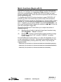
Metric Functions (Begin with X)
EndResult® functions which use metric engineering units begin with the
letter “X”. For example, to compute the enthalpy of steam at 13700 kPa
and 510°C, you would enter =XSTMPT2H(13700,510) and your result
would be 3355.246 kJ/kg. Notice that both the inputs and the result are in
metric engineering units.
The EndResult® ERUNITS function described on page “EREXCEL-45”
provides you with a convenient way to perform many unit conversions.
EndResult® functions require any percentage (e.g. percent quality, relative
humidity, etc.) to be entered into the worksheet as a number between 0
and 1. If desired, you can select “0.00%” from the Format Number… list
box to get Microsoft® Excel to display the number as a percent (or use the
quick key combination <CTRL-%>).
Remember that Microsoft® Excel allows you to adjust the number of
displayed digits by:
(1)
Adjusting the cell width of cells which have been formatted using
the Format Number… “General” command.
(2)
Specifying the number of decimal places when formatting a range
of cells using a fixed “0.00”, scientific “0.00E+00”, or percent
“0.00%” format.
Several EndResult® functions allow you to enter ‘Not Applicable’ for one
or more arguments in a function. As shown by the examples below, this
can be accomplished by entering either NA(), #N/A, or by leaving the
argument blank.
=XRADLOSS (1.5E+8,4,101000,30.5,10,1706,3396,1209,10200000,3023,3536,9250000,NA(),NA(),NA())
=XRADLOSS (1.5E+8,4,101000,30.5,10,1706,3396,1029,10200000,3023,3536,9250000,#N/A,#N/A,#N/A)
=XRADLOSS (1.5E+8,4,101000,30.5,10,1706,3396,1029,10200000,3023,3536,9250000,,,)
R
EndResult®
©2003 Sega Inc.
EREXCEL-3
November 1, 2002 - English
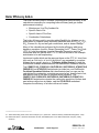
Attaching the EndResult® Hardware Key
The EndResult® hardware key sent with your EndResult® software should
support the Steam Plant Engineering Tools Add-in in addition to all other
EndResult® add-ins which you have purchased.
The hardware key should be attached to the parallel printer port (either
LPT1, LPT2, or LPT3) of your IBM PC/XT/AT, PS/2 or fully compatible
computer. If you are running EndResult® under Microsoft® Windows
NTTM, be sure to follow the instructions which start on page “Installation10”.
If the hardware key is incorrect or missing, the following differences will be
apparent:
(1)
When the EndResult® add-ins are loaded, a pop-up window will
notify you that the hardware key is missing.
(2)
All EndResult® functions within the Excel worksheet will return
“#Key?”.
If you have purchased the EndResult® Steam Plant Engineering Tools
Add-in and you are still having problems with your hardware key, please
contact Sega Inc. immediately.
If the hardware key is incorrect or missing for more than 15 seconds, any
subsequent attempt to recalculate an EndResult® function will return
“#KEY?”.
After the hardware key is attached, you can eliminate key errors in the
worksheet by either:
(1)
pressing F9 to recalculate the worksheet.
(2)
moving the pointer to each (“#Key?”) cell and pressing F2 followed
by <ENTER> to recalculate the cell.
(3)
moving the pointer to inputs in the calculation chain and pressing
F2 followed by <ENTER> to recalculate all cells which are dependent
on the input.
If any EndResult® function is displaying an error message (e.g. “#N/A”,
“#KEY?”, etc.), you can display a brief explanation for the error by moving
the cell pointer to the cell containing the error message and selecting
“EndResult®” from the Microsoft® Excel Help menu.
Note: The absence of the hardware key only affects EndResult®
functions. Microsoft Excel (as well as add-ins sold by other vendors) will
still function normally with or without the EndResult® hardware key.
Since the Steam Plant Engineering Tools Add-in is not copy protected,
you may make the number of backup copies of the add-in stipulated in the
preceding Software License Agreement. However, since only one key is
provided with each original copy, only one copy of the add-ins can be run
at any one time.
Male End of the
hardware key plugs
into the computer
parallel port.
R
Parallel Port
HARDWARE KEY
S74004
TM
EndResult
hardware key
Style One
Male End
R
Engineering Tools
On Line Tools
Communication
Parallel Port
HARDWARE KEY
S74004____________
R
EndResult
hardware key
Style Two
R
EndResult®
©2003 Sega Inc.
EREXCEL-4
November 1, 2002 - English
Installing the Add-in Files on Your Hard Disk
Please reference the latest readme file for installation instructions. This
can be found at www.endresult.com. Also available for download are the
Examples Spreadsheets and the Pre-Defined Spreadsheet Solutions.
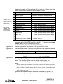
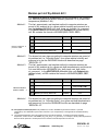
Identifying the Cause of an Error
If a cell containing an EndResult® Steam Plant Engineering Tools function
displays an error message (e.g., “#N/A”, “#KEY?”, etc.), you can move the
cell pointer to the cell and select “EndResult®” from the Microsoft® Excel
Help menu to display a brief explanation for why the error occurred.
Remember that you can select “EndResult®” from the Help menu by using
the mouse or by pressing <ALT>, “H”, “R” on the keyboard.
As shown in the example below, the error message displays the name of
the EndResult® Steam Plant Engineering Tools function which is evoking
an error and a brief explanation for why the error occurred. If the error is
being caused by the value of one or more arguments being passed to the
function, the error message will identify the argument(s) which are
responsible for the error.
!
Information for users
of Microsoft Excel
Version 3.0
"EndResult
" will not
appear in the Excel Help
menu if you have
selected "Short Menus".
If desired, you can
select "Full Menus" from
the Excel "Options"
menu to re-enable the
Help "EndResult
" menu
item.
Selecting "EndResult
"
from the Excel Help
menu will clear the
"Move Selection after
Enter" check box.
If desired, you can
select "Workspace..."
from the Excel Options
menu to re-enable this
item.
R
If you enter a number which is above the maximum allowable, the
function will return a “#N/A” error. As shown in the picture below, you
can display the maximum on your screen by moving your pointer to the
cell and selection “EndResult®” from the Microsoft® Excel Help menu.
Then, select "EndResult"
to view explanation.
Move pointer
to error cell.
Microsoft Excel
Help
File Edit Formula Format Format Data Options Macro Window
Index
Normal
Keyboard
E80
=WETPQ2V($B$77,$B$81)
Lotus 1-2-3...
A
B
C
D
E
F
G
H
Multiplan...
66
Tutorial
Press.=
3000 Psia
Density= 54.5467417
67
Lb/Cuft
LIQPT2D(P,T)
About...
min:
0.088589
Enthalpy= 378.4749569 Btu/Lb
68
LIQPT2H(P,T)

max:
15500
Entropy= 0.559661
69
Btu/Lb ˚R EndResult
LIQPT2S(P,T)
Viscosity= 9.09223E-05 Lb/Sec-ft
70
LIQPT2U(P,T)
Temp.=
400 Deg ˚F
Spec.
Vol.= 0.018332901
71
Cuft/Lb
LIQPT2V(P,T)
Microsoft
Excel
min:
32
72
Spec. Heat= 1.054752439 Btu/Lb ˚F
LIQPT2C(P,T)
ERRORS
max:
0.391063397 Btu/Hr ft ˚F LIQPT2K(P,T)
705.47
73
Ther.Cond.=
WETPQ2V(Arg#1): Maximum for Pressure is 3208.23476 Psia.
74
20000 Psia.)
WET (You entered
75
(Saturated
steam a given pressure and quality)
76
Press.=
77
20000 Psia
Density= #N/A
Lb/Cuft
WETPQ2D(P,Q)
78
0.088589
Enthalpy= OK#N/A
Btu/Lb
WETPQ2H(P,Q)
min:
79
max:
3208.235
Entropy= #N/A
Btu/Lb ˚R
WETPQ2S(P,Q)
80
Temp.= #N/A
Deg ˚F
WETPQ2T(P,Q)
81
Qual.=
55.0%
Viscosity= #N/A
Lb/Sec-ft
WETPQ2U(P,Q)
82
min:
0.0%
Spec. Vol.= #N/A
Cuft/Lb
WETPQ2V(P,Q)
83
max:
100.0%
Spec. Heat= #N/A
Btu/Lb ˚F
WETPQ2C(P,Q)
EndResult®
©2003 Sega Inc.
EREXCEL-5
November 1, 2002 - English
If you enter a number which is below the minimum allowable, the function
will return a "#N/A" error. If desired, you can display the minimum on
your screen by moving your pointer to the cell and selecting
"EndResult®" from the Microsoft® Excel Help menu.
! If the hardware key is incorrect or missing, the function will return a
"#KEY?" error. You can determine if the hardware key is causing the
problem by moving your pointer to the cell and selecting "EndResult®"
from the Microsoft® Excel Help menu.
! If you select "EndResult®" from the Microsoft® Excel Help menu while
your pointer is on a cell which does not contain an error (or warning),
the EndResult® pop-up window wil tell you that there is "No Error or
Warning in this Cell!".
! If you select "EndResult®" from the Microsoft® Excel Help menu while
your pointer is on a cell which does not contain an EndResult®
function, the pop-up window will tell you that there is "No EndResult®
function in this cell!".
! If cells with EndResult® functions display “#REF!” or if you select
"EndResult®" from the Microsoft® Excel Help menu and a pop-up
window does not appear, the EndResult® add-in is not properly
installed.
! You cannot access Help EndResult® messages if your document is
protected AND your cell pointer is on a locked cell. You must either
unprotect the document or unlock the cell before selecting
"EndResult®" from the Microsoft® Excel Help menu.
Using Warnings
EndResult® functions can also provide information in the form of
“Warnings”. Whereas an error causes an EndResult® function to return
an error message (e.g., "#N/A", "#KEY?", etc.), a warning still allows the
function to compute a result.
To determine if an EndResult® function is causing a warning, move the
cell pointer to the cell and select "EndResult®" from the Help menu. This
will cause either a list of warnings or the message "No error or warning in
this cell" to appear. Remember that you can select "EndResult®" from
the Help menu by using the mouse or by pressing <ALT>, "H", "R" on the
keyboard.
Lastly, if an EndResult® function evokes one or more errors and one or
more warnings, the errors will always be listed first.
R
EndResult®
©2003 Sega Inc.
EREXCEL-6
November 1, 2002 - English
Add-in Functions
Mixed Gas Thermo-Physical Property Add-in
The results computed by the “Mixed Gas Thermo-Physical Properties”
add-in are based on formulations from the following sources:
!
The ultimate analysis computation method, the molecular weights, and the
energy conversion constants used by this add-in are based on data and
equations found in Steam/Its Generation and Use4.
! The gas compressibility is computed using the Redlich-Kwong method.
! Viscosity is computed using “Arnolds Correlation” and the square root rule.
! Critical properties computed by this add-in are based on formulations found in
the Flow Measurement Engineering Handbook5.
! Enthalpy and entropy of water vapor are from the ASME Steam Tables6.
! Additional gas properties are computed from formulations found in the
Physical and Thermodynamic Properties of Pure Chemicals7,
Thermodynamics8, Fan Engineering9, and the ASHRAE10 Psychrometric
Charts.
Both the COMBCYC.XLS and GASTURB.XLS worksheets (provided in the
www.endresult.com Pre-defined Spreadsheet Solutions download file)
demonstrate how the mixed gas thermo-physical property add-in functions
can be combined with other functions to compute boiler efficiency, gas
turbine heat rate, and properties of the combustion air and flue gas.
For a working example of all of the mixed gas thermo-physical property
functions shown below, load the MIXGAS.XLS worksheet (provided in the
www.endresult.com Examples download file). The MIXGAS.XLS worksheet
provides an easy way to familiarize yourself with each EndResult®
function. You can experiment with each function by entering numbers into
the highlighted unprotected user-input cells.
The MIXGAS.XLS worksheet from your EndResult® Examples download file
is shown below and on the following pages. The name of each argument
appears in cells A1 to A13 and an example value for each argument
appears in cells B1 to B13. Valid ranges for each input are listed in
column C.
A
The second argument can
Be either Temperature,
Enthalpy, or Entropy.
See the following page
For more information
"
1
Pressure
2
Temperature
B
C
14.696
(from 2.25E-14 to 3208.235 Psia)
364.0922
(from -425°°F to 4000°°F)
3
_____________________
4
Babcock & Wilcox. Steam/Its Generation and Use, 40th Edition, (New York: Babcock & Wilcox Company, 1992),
Section 6.
5 Richard W. Miller. Flow Measurement Engineering Handbook, (New York: McGraw-Hill Book Company, 1983).
6 International Formulation Committee, “The 1967 Formulation for Industrial Use”, ASME Steam Tables, Fifth Edition, (New
York: American Society of Mechanical Engineers, 1873), Appendix 1, pages 11-29.
7 T.E. Daubert and R.P. Danner, ed., Physical and Thermodynamic Properties of Pure Chemicals, Data Compilation, (New
York: Hemisphere Publishing Corporation, 1991).
8 Faires, Thermodynamics (New York: The MacMillan Company, 1957).
9 Fan Engineering, (New York: Buffalo Forge Company, 1983).
10 ASHRAE Psychrometric Chart No. 1 & No. 2, American Society of Heating, Refrigerating, and Air-Conditioning Engineers,
Inc., 1963.
R
EndResult®
©2003 Sega Inc.
EREXCEL-7
November 1, 2002 - English
The items in rows 4 to 13 are optional. If you omit any of these items, the
default value shown to the left of each row will be used.
A
(default is Temperature) →
(default is 60°°F)
→
(default is 14.73 Psia) →
4
Second Argument
5
Reference Temperature
B
C
Temperature
60
(from -425°°F to 4000°°F)
6
Reference Pressure
(applies to enthalpy and →
entropy, default is 32.018°°F)
7
Zero Enthalpy Temperature
→
8
Gas Mixture Percent by
9
Carbon Dioxide
11.4940%
(from 0% to 100% by Volume or Weight)
10
Atmospheric Nitrogen
74.0720%
(from 0% to 100% by Volume or Weight)
11
Oxygen
6.4000%
(from 0% to 100% by Volume or Weight)
12
Sulfur Dioxide
0.1320%
(from 0% to 100% by Volume or Weight)
13
Water Vapor
7.9020%
(from 0% to 100% by Volume or Weight)
(default is Volume)
Use a formula like
SUM($B$9 : $B$13) to
ensure that 100% of
the gas constituents
have been specified.
14.73
(Temperature, Enthalpy, or Entropy)
32.018
Volume
(from 2.25E-14 to 3208.235 Psia)
(from -425°°F to 4000°°F)
(Weight or Volume)
14
15
Ultimate Analysis Carbon GAS2CAR
4.683946%
% by Wt
Each mixed gas thermo-physical property function requires the same four
arguments as the GAS2CAR function in cell B15. To compute the Ultimate
Analysis Carbon, cell B15 contains the formula
=GAS2CAR($B$1,$B$2,$A$4:$A$13,$B$4:$B$13).
The first argument is the pressure of the gas mixture in Psia.
The “Second Argument” identifier shown above in row 4 specifies whether
the second argument is temperature, enthalpy, or entropy.
Argument #1
Argument #2
If you specify Second Argument as:
Enter a value for the 2nd argument which is:
Temperature........................................................ from -425°F to 4000°F
Enthalpy ........................................................ from -1300 to 3400 Btu/Lb.
Entropy........................................................from -1.27 to 2.21 Btu/Lb °R
Argument #3
The third argument is the Identifier Range. In the example spreadsheet
above the Identifier Range extends from cell A4 to A13 and includes five
gases. The Identifier Range must be a single column wide. As a
minimum, the Identfier Range must include from 1 to 37 of the following
gases:
Acetylene, Air, Ammonia, Argon, Benzene, Carbon Dioxide, Carbon Monoxide, Ethane, Ethyl Alcohol,
Ethylene, Hydrogen Gas, Hydrogen Sulfide, i-Butane, 1-Butene, i-Pentane, Methane, Methyl Alcohol, nButane, cis-2-Butene, n-Heptane, n-Hexane, n-Nonane, n-Octane, n-Pentane, 1-Pentene, Neopentane,
Nitrogen, Atmospheric Nitrogen, Oxygen, Propane, Propylene, Sulfur Dioxide, Toluene, o-Xylene, mXylene, p-Xylene, Water Vapor.
Identifiers can be abbreviated to as few as 3 characters (e.g. “Ben” for
“Benzine”), as long as enough characters of each identifier are entered to
R
EndResult®
©2003 Sega Inc.
EREXCEL-8
November 1, 2002 - English
distinguish it from other identifiers. Each identifier may be left, center, or
right justified. Although capitalization is not significant, hyphens should be
included where shown. An Identifier can be followed by a comment as
long as a non-alphanumeric character (e.g. comma, semicolon,
parenthesis, colon, …) precedes the comment. The Identifier and Value
Ranges can include blank rows.
The fourth argument is the Value Range. In the example spreadsheet
above the Value Range extends from cell B4 to B13 and includes five
gases. The Value Range must be a single column wide.
If your identifier is a gas, its percent by volume or weight should be
entered into the worksheet as a number from 0 to 1. If desired, you can
select “0.00%” from the Format Number… list box to get Microsoft® Excel to
display the number as a percent (or use the quick key combination <CTRL%>). Omitted gases are automatically assigned zero percent.
Argument #4
WARNING:
Under conditions of very low temperature and/or high pressure one or more of
the gas constituents may become liquid. Under marginal conditions, you should
use the GAS2ZRA function described on page "EREXCEL-14" to insure that the
answer returned by the add-in is valid. If the GAS2ZRA function tells you that a
constituent in the gas mix is in the liquid state at the zero enthalpy, reference,
and/or actual conditions, the results computed by the add-in may not be valid.
The "ZR" exception for "Water Vapor": As shown in the example worksheet on
page "EREXCEL-14", cell F78 contains the formula =GAS2ZRA($B$1, $B$2,
$A$4 : $A$13, $B$4 : $B$13, “Water Vapor”). For most common combustion air
and flue gas applications, if you ask the GAS2ZRA function for the state of H2O,
the letters returned by the GAS2ZRA function will include “Z” and “R” indicating
that H2O is a liquid at both the zero enthalpy conditions and reference conditions.
Since the mixed gas add-in is linked to the ASME steam tables, the enthalpy and
entropy contribution from H2O should still be correct even if H2O is a liquid at
these conditions. However, if one of the letters returned by the GAS2ZRA
function is a letter ”A” (i.e. actual conditions), the results computed by the add-in
may not be valid.
Notice to users of previous versions
of the EndResult add-ins.
The GAS2H2O function for computing Ultimate Analysis Moisture is obsolete and
should not be used. To insure compatibility with worksheets developed using
previous versions of EndResult, the GAS2H2O function will ALWAYS return zero
and will not return an error.
Additionally, the "Analysis Compensated (or Uncompensated)" option is obsolete
and should not be used. To insure compatibility with worksheets developed
using previous versions of EndResult, any appearance of "Analysis
Compensated (or Uncompensated)" within a mixed gas calculation will be
ignored and the analysis will ALWAYS be uncompensated.
R
EndResult®
©2003 Sega Inc.
EREXCEL-9
November 1, 2002 - English
To compute the ultimate analysis carbon, cell B15 contains the formula
=GAS2CAR($B$1, $B$2, $A$4:$A$13, $B$4:$B$13). The GAS2CAR
function uses the four arguments described on pages “EREXCEL-8” and
"ÉREXCEL-9”. The results in cells B16 through B20 are computed in a
similar manner using the same arguments and the function indicated in
column A.11
A
B
C
15
Ultimate Analysis Carbon
GAS2CAR
4.683946%
% by Wt
16
Ultimate Analysis Hydrogen
GAS2HYD
.540460%
% by Wt
17
Ultimate Analysis Oxygen
GAS2OXY
23.859626%
% by Wt
18
Ultimate Analysis Nitrogen
GAS2NIT
70.772360%
% by Wt
19
Ultimate Analysis Sulfur
GAS2SUL
0.143609%
% by Wt
20
Ultimate Analysis Total
GAS2TOT
100.000000%
% by Wt
To compute the higher heating value, cell B22 contains the formula
=GAS2HHVSCF($B$1, $B$2, $A$4:$A$13, $B$4:$B$13). The
GAS2HHVVSCF function uses the four arguments described on pages
"EREXCEL-8” and “EREXCEL-9”. The results in cells B23 through B28
are computed in a similar manner using the same arguments and the
function indicated in column A.
A
B
C
Standard Conditions→
22
Higher Heating Value (Reference, SCF)
GAS2HHVSCF
0
Btu/Cuft
Actual Conditions→
23
Higher Heating Value (ACF)
GAS2HHVACF
0
Btu/Cuft
24
Higher Heating Value
GAS2HHV
0
Btu/Lb
Standard Conditions→
25
Lower Heating Value (Reference, SCF)
GAS2LHVSCF
0
Btu/Cuft
Actual Conditions→
26
Lower Heating Value (ACF)
GAS2LHVACF
0
Btu/Cuft
27
Lower Heating Value
GAS2LHV
0
Btu/Lb
28
Theoretical Air per Lb As Fired Fuel
GAS2AIR
0
Lb/Lb
_______________________
11 Hint: To quickly enter the cell formulas in cells B15 to B20, enter the GAS2CAR function in cell B15, then copy it to cells
B16 to B20, and then change each cell to the correct function. Correct use of absolute references (e.g. $B$2) and relative
references (e.g. B2) will ensure that copied formulas have the desired references.
R
EndResult®
©2003 Sega Inc.
EREXCEL-10
November 1, 2002 - English
To compute the reduced temperature, cell B30 contains the formula
=GAS2RT($B$1, $B$2, $A$4:$A$13, $B$4:$B$13). The GAS2RT
function uses the four arguments described on pages “EREXCEL-8” and
"ÉREXCEL-9”. The remaining results in cells B31 through B35 are
computed in a similar manner using the same arguments and the function
indicated in column A.12
A
B
C
30
Reduced Temperature
GAS2RT
2.4090887
31
Reduced Pressure
GAS2RP
1.863681E-2
32
Critical Temperature
GAS2TC
341.93934
°R
33
Critical Pressure
GAS2PC
788.54691
Psia
34
Critical Volume
GAS2VC
4.821743E-02
35
Critical Compressibility
GAS2ZC
0.2846665
Cuft/Lb
[Zc]
The following 6 items are only results if water vapor is present, otherwise
these items will return “#N/A”. To compute the water vapor partial
pressure, cell B37 contains the formula =GAS2H2OPP($B$1, $B$2,
$A$4:$A$13, $B$4:$B$13). The GAS2H2OPP function uses the four
arguments described on pages “EREXCEL-8” and “EREXCEL-9”. The
remaining results in cells B38 through B42 are computed in a similar
manner using the same arguments and the function indicated in column A.
A
Dew point "
temperature is only
computable if the gas
temperature is
between -80°F and
705.47°F, otherwise
GAS2DPT will return
”#N/A”.
B
1.161278
C
37
Water Vapor Partial Pressure
GAS2H2OPP
Psia
38
Water Vapor ASME Enthalpy at Partial Pressure
GAS2H2OHPP 1225.143
Btu/Lb
39
Water Vapor ASME Entropy at Partial Pressure
GAS2H2OSPP 2.1359245
Btu/Lb °R
40
Water Vapor Contribution to Specific Enthalpy
GAS2H2OH
59.17336
Btu/Lb
41
Water Vapor Contribution to Specific Entropy
GAS2H2OS
.1031634
Btu/Lb °R
42
Water Vapor Dew Point Temperature
GAS2DPT
106.7905
°F
______________________
12 Hint: To quickly enter the cell formulas in cells B30 to B35, enter the entire GAS2RT function in cell B30, then copy it to
cells B31 to B35, and then change each cell to the correct function. Correct use of absolute references (e.g. $B$2) and
relative references (e.g. B2) will ensure that copied formulas have the desired references.
R
EndResult®
©2003 Sega Inc.
EREXCEL-11
November 1, 2002 - English
To compute the water saturation vapor pressure, cell B44 contains the
formula =GAS2SATP($B$1, $B$2, $A$4:$A$13, $B$4:$B$13). The
GAS2SATP function uses the four arguments described on pages
“EREXCEL-8” and “EREXCEL-9”. The remaining results in cells B45
through B50 are computed in a similar manner using the same arguments
and the function indicated in column A.13
A
These items are
computable if the
→
temperature is between
-80°F and 705.47°F,
→
otherwise they will return
“#N/A”.
→
Wet-bulb temperature is
computable if only air and
perhaps water vapor are →
present and if the gas
temperature is between -80°F
and 200°F, otherwise
GAS2WB will return “#N/A”.
44
Water Saturation Vapor Pressure
45
Degree of Water Saturation
46
B
GAS2SATP
14
C
161.0886
Psia
GAS2H2OSAT -7.797244%
Percent
Relative Humidity (Water Vapor in Dry Gas)
GAS2RH
.7208939%
Percent
47
Humidity Ratio (Water Vapor in Dry Gas)
GAS2HMR
5.330768E-2
Lb/Lb
48
Specific Humidity (Water Vapor in Moist Gas)
GAS2HMS
4.829916E-2
Lb/Lb
49
Absolute Humidity (Water Vapor in Moist Gas) GAS2HMA
2.367001E-3
Lb/Cuft
50
Thermodynamic Wet-Bulb Temperature
#N/A
°F
GAS2WB
To compute the Molecular Weight, cell B52 contains the formula
=GAS2MW($B$1, $B$2, $A$4:$A$13, $B$4:$B$13). The GAS2MW
function uses the four arguments described on pages “EREXCEL-8” and
“EREXCEL-9”. The remaining results in cells B53 through B56 are
computed in a similar manner using the same arguments and the function
indicated in column A.
A
B
52
Molecular Weight
53
Specific Gravity (Molecular Weight Ratio)
54
Specific Gravity (Density Ratio) (Reference)
55
Specific Gravity (Density Ratio)
56
Specific Heat [Cp]18 (Ideal Gas)
15
16
17
C
GAS2MW
29.47396
GAS2SGMW
1.017536
[G]
GAS2SGREF
1.0187097
[G]
GAS2SG
.6401903
[G]
GAS2C
.2562904
Btu/Lb °F
______________________
13 Hint: To quickly enter the cell formulas in cells B44 to B50, enter the entire GAS2SATP function in cell B44, then copy it
to cells B45 to B50, and then change each cell to the correct function. Correct use of absolute references (e.g. $B$2) and
relative references (e.g. B2) will ensure that copied formulas have the desired references.
14 When saturation vapor pressure is greater than the total gas pressure as occurs with high temperature flue gas, and the
relative humidity is greater than 0.00, the degree of saturation can be negative (See reference 7, page 1-15, equation
1.24).
15 The specific gravity value may be unrealistic if it is greater than 5.
16 The specific gravity value may be unrealistic if it is greater than 5.
17 The specific gravity value may be unrealistic if it is greater than 5.
18 If you need a faster method for computing the specific heat of flue gas, the GASTR2C function on page “EREXCEL-24”
provides a fast and simple way to obtain an approximate value for the specific heat of flue gas at 14.696 psia.
R
EndResult®
©2003 Sega Inc.
EREXCEL-12
November 1, 2002 - English
To compute the ratio of specific heats, cell B58 contains the formula
=GAS2CR($B$1, $B$2, $A$4:$A$13, $B$4:$B$13). The GAS2CR
function uses the four arguments described on pages “EREXCEL-8” and
“EREXCEL-9”. The remaining results in cells B59 through B70 are
computed in a similar manner using the same arguments and the function
indicated in column A.
A
B
C
58
Ratio of Specific Heats (Ideal Gas)19
GAS2CR
1.357678
[Cp/Cv]
59
Temperature (Dry Ideal Gas + H2 O ASME)
GAS2TEMP
364.0922
°F
60
Specific Enthalpy (Dry Ideal Gas + H2 O ASME) GAS2ENTH20
135.2667
Btu/Lb
61
Specific Entropy (Dry Ideal Gas + H2 0 ASME)
GAS2ENTR20
.2211987
Btu/Lb °R
62
Compressibility Factor (Reference)21
GAS2Z0
0.9982604
[Z0]
63
Compressibility Factor22
GAS2Z1
0.9997867
[Z1]
64
Super Compressibility
GAS2SZ
1.000107
[Fpv]
65
Density (Reference)23
GAS2DR
7.798304E-2
Lb/Cuft
66
Density24
GAS2D
4.900708E-2
Lb/Cuft
67
Specific Volume (Reference)
GAS2RVOL
12.823300
Cuft/Lb
68
Specific Volume
GAS2VOL
20.405214
Cuft/Lb
69
Viscosity (Dry Ideal Gas)
GAS2U
1.572015E-05
Lb/Sec-ft
70
Viscosity (Dry Ideal Gas)
GAS2UC
2.339416E-02
Centipoise
Entering Gage Pressures
EndResult® functions require that all pressures to be entered as absolute
pressures. If, however, you have a value in gage pressure (e.g. 1500
psig), simply add the atmospheric pressure (e.g. 14.696 psia) to the gage
pressure as shown by the gas density calculation below:
=GAS2D(1500+14.696,300,$A$4:$A$13,$B$4:$B$13)
______________________
19 The specific heat ratio may be unrealistic if it is less than 0.1 or greater than 4.
20 Enthalpy and entropy calculations are based on a change in enthalpy or entropy from the zero enthalpy temperature,
which can be modified as shown on page “EREXCEL-8”.
21 The compressibility factor (reference) may be unrealistic if it is greater than 1.24.
22 The compressibility factor may be unrealistic if it is greater than 1.24.
23 The density (reference) value may be unrealistic if it is greater than 100.
24 The density value may be unrealistic if it is greater than 100.
R
EndResult®
©2003 Sega Inc.
EREXCEL-13
November 1, 2002 - English
PCTBYVOL, PCTBYWT, GAS2PP, GAS2TSAT, and GAS2ZRA
Function
Computes an Individual Gas
PCTBYVOL.......... Percent by volume of the total gas mixture
PCTBYWT ........... Percent by weight of the total gas mixture
GAS2PP .............. Partial pressure
GAS2TSAT .......... Temperature of saturation
GAS2ZRA ............ State at zero enthalpy, reference, and actual temp.
All five functions above require the same five arguments:
The first four arguments are the same as those listed on pages
“EREXCEL-8” and “EREXCEL-9”.
The fifth argument must be one of the following gas names:
Arguments
#1 to #4
Argument #5
Acetylene, Air, Ammonia, Argon, Benzene, Carbon Dioxide, Carbon Monoxide,
Ethane, Ethyl Alcohol, Ethylene, Hydrogen Gas, Hydrogen Sulfide, i-Butane,
1-Butene, i-Pentane, Methane, Methyl Alcohol, n-Butane, cis-2-Butene, n-Heptane,
n-Hexane, n-Nonane, n-Octane, n-Pentane, 1-Pentene, Neopentane, Nitrogen,
Atmospheric Nitrogen, Oxygen, Propane, Propylene, Sulfur Dioxide, Toluene,
o-Xylene, m-Xylene, p-Xylene, Water Vapor.
For example, to compute the percent by volume of carbon dioxide of the
total gas mixture, cell B74 below contains the formula =PCTBYVOL($B$1,
$B$2, $A$4:$A$13, $B$4:$B$13, “Carbon Dioxide”). Similar formulas are
used to compute the values in cells B74 through F78.
A
B
C
D
E
F
72
% Volume
% Weight
Part Psia
Sat Temp (°F)
ZRA
73
=PCTBYVOL
=PCTBYWT
=GAS2PP
=GAS2TSAT
=GAS2ZRA
74
Carbon Dioxide
11.4940%
17.1626%
1.689
-164.54
____
75
Atmospheric Nitrogen
74.0720%
70.7724%
10.886
-324.35
____
76
Oxygen
6.4000%
6.9482%
0.941
-331.64
____
77
Sulfur Dioxide
0.1320%
0.2869%
0.019
-148.07
____
78
Water Vapor
7.9020%
4.8299%
1.161
106.79
ZR_
Under conditions of very low temperature and/or high pressure, one or
more of the gas constituents may become liquid. If this happens for other
than water vapor, your mixed gas results will not be valid (See warning on
page "EREXCEL-9”). The GAS2ZRA function should be used if you are
uncertain as to whether or not ALL of the constituents in the gas mixture
will be a gas at the specified pressures and temperatures.
The GAS2ZRA function returns one or more of the following letters:
“Z" If the constituent is not a gas at zero enthalpy conditions
“R” If the constituent is not a gas at reference conditions
“A” If the constituent is not a gas at actual conditions
R
EndResult®
©2003 Sega Inc.
EREXCEL-14
November 1, 2002 - English
Computing Psychrometric Properties Using Relative Humidity
The worksheet below demonstrates how to compute the properties of
atmospheric air with a given relative humidity.
A
B
C
D
E
100
Pressure
12
(from .9492356 to 15.472 Psia)
101
Dry Bulb Temperature
100
(from -80°° F to 200°° F)
103
Relative Humidity
80%
(from 0% to 100%)
104
Zero Enthalpy Temperature
F
102
(applies to enthalpy and entropy,
default is 32.018°F)
→
40
(from -425°°F to 4000°° F)
105
(Water Vapor in Dry Air) →
(Water Vapor in Moist Air) →
(Water Vapor in Moist Air) →
(Ideal Gas)
Wet Bulb Temperature
GAS2WB
107
Reference Pressure
GAS2REFP
14.696
108
Reference Temperature
GAS2REFT
60
109
Humidity Ratio
GAS2HMR
4.197367E-2
Lb/Lb
110
Specific Humidity
GAS2HMS
4.032289E-2
Lb/Lb
111
Absolute Humidity
GAS2HMA
2.279395E-03
Lb/Cuft
112
Specific Heat [Cp]
25
93.701501
°F
106
Psia
°F
GAS2C
.24830705
Btu/Lb ° F
113
% Volume
% Weight
Part Psia
Sat. Temp. (°° F)
ZRA
114
=PCTBYVOL
=PCTBYWT
=GAS2PP
=GAS2TSAT
=GAS2ZRA
→
115
Air
93.6718%
95.9677%
11.241
-321.42
___
116
Water Vapor
6.3282%
4.0323%
0.759
92.70
Z__
To compute the Wet Bulb Temperature26, cell C106 contains the formula:
=GAS2WB($C$100,$C$101,$A$103:$A$104,$C$103:$C$104).
=GAS2WB (air_pressure, dry_bulb_temp, Ident_Range, Value_Range)
The same arguments (as shown in the GAS2WB function above) can be used to
perform the calculations shown in rows 107 through 116. The first two
arguments must be the pressure and dry-bulb temperature of the atmospheric air
and the last two arguments must be the Identifier and Value Ranges respectively
in which you have specified the Relative Humidity. The only other item which you
are allowed to specify in your Identifier and Value Ranges is the Zero Enthalpy
Temperature. (A Zero Enthalpy Temperature of 32.018°F will be used if not otherwise
specified.) For more detailed instructions on specifying the Identifier and Value
Ranges, see pages “EREXCEL-8” and “EREXCEL-9”.
__________________________
25 If you need a faster method for computing the specific heat of air, the AIRT2C function on page “EREXCEL-24” provides a
fast and simple way to obtain an approximate value for the specific heat of air at 14.696 psia.
26 For a chart of relative humidity versus dry bulb temperature and wet bulb temperature, see the ASHRAE Psychrometric
Chart No. 1 (Normal Temperature)” and “ASHRAE Psychrometric Chart No. 2 (Low Temperature)” in the appendix of the
Boiler Efficiency chapter.
R
EndResult®
©2003 Sega Inc.
EREXCEL-15
November 1, 2002 - English
Computing Psychrometric Properties Using Wet Bulb Temperature
The worksheet below demonstrates how to compute the properties of
atmospheric air with a given wet bulb temperature.
A
B
C
D
E
F
130
Pressure
12
(from 1.274955 to 15.472 Psia)
131
Dry Bulb Temperature
110
(from -80°°F to 200°°F)
133
Wet Bulb Temperature
90
(from 56.7658°°F to 110°°F)
134
Zero Enthalpy Temperature
132
(applies to enthalpy and entropy,
default is 32.018°F)
→
32.018
(from -425°°F to 4000°°F)
135
136
Relative Humidity
GAS2RH
48.65026%
137
Reference Pressure
GAS2REFP
14.696
138
Reference Temperature
GAS2REFT
60
Percent
Psia
°F
(Water Vapor in Dry Air)
→
139
Humidity Ratio
GAS2HMR
3.386498E-2
Lb/Lb
(Water Vapor in Moist Air)
→
140
Specific Humidity
GAS2HMS
3.278852E-2
Lb/Lb
(Water Vapor in Moist Air)
→
141
Absolute Humidity
GAS2HMA
1.828890E-3
Lb/Cuft
(Ideal Gas)
→
142
Specific Heat [Cp]
27
GAS2C
.24681362
Btu/Lb ° F
143
% Volume
% Weight
Part Psia
Sat. Temp. (°°F)
ZRA
144
=PCTBYVOL
=PCTBYWT
=GAS2PP
=GAS2TSAT
=GAS2ZRA
145
Air
94.8311%
96.7211%
11.380
-321.26
____
146
Water Vapor
5.1689%
3.2789%
0.620
86.26
Z__
To compute the Relative Humidity28, cell C136 contains the formula:
=GAS2RH($C$130,$C$131,$A$133:$A$134,$C$133:$C$134).
=GAS2RH (air_pressure, dry_bulb_temp, Ident_Range, Value_Range)
The same arguments (as shown in the GAS2RH function above) can be used to perform the
calculations shown in cells rows 137 through 146. The first two arguments must be the pressure
and dry-bulb temperature of the atmospheric air and the last two arguments must be the Identifier
and Value Ranges in which you have specified the Wet Bulb Temperature29. The only other item
which you are allowed to specify in you Identifier and Value Ranges is the Zero Enthalpy
Temperature. (A Zero Enthalpy Temperature of 32.018°F will be used if not otherwise
specified.) For more detailed instructions on specifying the Identifier and Value Ranges, see pages
“EREXCEL-8” and ”EREXCEL-9”.
______________________
27 If you need a faster method for computing the specific heat of air, the AIRT2C function on page “EREXCEL-24” provides a
fast and simple way to obtain an approximate value for the specific heat of air at 14.696 psia.
28 For a chart of relative humidity versus dry bulb temperature and wet bulb temperature, see the ”ASHRAE Psychrometric
Chart No. 1 (Normal Temperature)” and “ASHRAE Psychrometric Chart No. 2 (Low Temperature)” in the appendix of the
Boiler Efficiency chapter.
29- The wet-bulb temperature cannot be greater than the dry-bulb temperature. To obtain the minimum wet-bulb
temperature, use the function =WETTEMP (dry_bulb_temp, 0, air_pressure). For example, if the dry-bulb temperature is
110°F and the air pressure is 14.696 psia, then the minimum wet-bulb temperature is 60.419°F.
R
EndResult®
©2003 Sega Inc.
EREXCEL-16
November 1, 2002 - English
Steam and Water Property Add-in
The steam and water property add-in includes functions for computing a
variety of steam and water properties including: density, entropy,
enthalpy, viscosity, pressure, temperature, quality, specific heat, ratio of
specific heats, thermal conductivity, specific volume, saturation pressure,
and saturation temperature.
EndResult®’s steam and water property calculations are based on
formulations found in ASME Steam Tables30 and are similar to those
described in the “Steam Tables Properties” chapter. Each function has
been tested to ensure that it produces the same values as the ASME
Steam Tables.
All of the EndResult® steam and water property functions use a similar
format to the example shown below:
From left to right, each function must have:
# 3 letters symbolizing the state
# 1 letter symbolizing the 1st input
# 1 letter symbolzing the 2nd input
# a number “2” symbolizing “TO”
# 1 letter symbolizing the result
# 2 arguments which you specify
Like bult-in Microsoft® Excel functions, each EndResult® function can be
pasted into the spreadsheet by selecting Paste Function… from the
Formula menu.
____________________
30 International Formulation Committee, “The 1967 Formulation for Industrial Use”, ASME Steam Tables, Fifth Edition,
(New York: American Society of Mechanical Engineers, 1983), Appendix 1, pages 11-29.
R
EndResult®
©2003 Sega Inc.
EREXCEL-17
November 1, 2002 - English
EndResult® functions require that all pressures be entered as absolute
pressures. If, however, you have a value in gage pressure (e.g. 1500
psig), simply add the atmospheric pressure (e.g. 14.7 psia) to the gage
pressure as shown by the liquid density calculation below:
=LIQPT2D(1500+14.7,300)
If you are interested in the properties of a particular steam or water state,
select your function from the “State-specific” functions shown on page
“EREXCEL-20”.
If you are unconcerned about the state of the steam and simply want to
know the properties of any steam or water, select your function from the
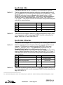
“Universal” functions shown on page “EREXCEL-19”.
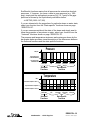
The pressure and temperature minimums and maximums shown by the
bar graphs below provide a visual description of the differences between
the universal functions and the state-specific functions.
Pressure
15500 psia
Critical Point Pressure
= 3208.2347600665 Psia
Triple Point Pressure
= 8.858914E-02 Psia
Any Steam
or Water (ANY)
Liquid
(LIQ)
Saturated
Steam (WET)
Universal
Functions
Superheated
Steam (STM)
Supercritical
Steam (CRT)
State-specific
Functions
Temperature
1500 ˚F
Critical Point Temperature = 705.47 ˚F
Any Given Saturation Temperature
Triple Point Temperature = 32.018 ˚F
Any Steam
or Water (ANY)
Liquid
(LIQ)
Universal
Functions
R
EndResult®
©2003 Sega Inc.
Saturated
Steam (WET)
Superheated
Steam (STM)
Supercritical
Steam (CRT)
State-specific
Functions
EREXCEL-18
November 1, 2002 - English
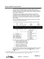
Steam and Water Property Universal Functions
The chart below describes the universal functions for calculating steam
and water properties:
P3pt
T3pt
PCpt
TCpt
TSat
=Triple point pressure
=Triple point temperature
=Critical point pressure
=Critical point temperature
=Saturation temperature
Function & Inputs
=ANYPT2…(P, T)
P=Pressure
(from P3pt to 15500 psia)
T=Temperature
(from T3pt°F to 1500°F)
=ANYPQ2… (P, Q)
Note: The ratio of
specific heats is not
available under the
conditions described in
the appendix of the
Flow Measurement
chapter on page
“Flow-A4”.
P=Pressure
(from P3pt to PCpt psia)
Q=Quality
(from 0% to 100%,
enter as 0 to 1)
=ANYPH2…(P, H)
P=Pressure
(from P3pt to 15500 psia)
H=Enthalpy of liquid at T3pt to
enthalpy of superheated
steam at 1500 °F in Btu/Lb
=ANYPS2…(P, S)
P=Pressure
(from P3pt to 15500 psia)
S=Entropy of liquid at T3pt to
entropy of superheated
steam at 1500°F in
Btu/Lb °R
R
=8.858914E-02 psia
=32.018°F
=3208.2347600665 psia
=705.47°F
=°F
Result
Units
Example
…D
…H
…S
…C
…R
…V
…K
…U
Density
Enthalpy
Entropy
Specific Heat [Cp]
Ratio of Specific
Heats
Specific Volume
Thermal Conductivity
Viscosity
Lb/Cuft
Btu/Lb
Btu/Lb °R
Btu/Lb °F
[Cp/Cv]
Cuft/Lb
Btu/Hr ft °F
Lb/Sec-ft
To obtain the entropy
of an H2O substance at
6000 psia and 200 °F,
enter =ANYPT2S
(6000,200) and the
result will be
0.287028 Btu/Lb °R.
…D
…H
…S
…C
…R
…V
…T
…K
…U
Density
Enthalpy
Entropy
Specific Heat [Cp]
Ratio of Specific
Heats
Specific Volume
Temperature
Thermal Conductivity
Viscosity
Lb/Cuft
Btu/Lb
Btu/Lb °R
Btu/Lb °F
[Cp/Cv]
Cuft/Lb
°F
Btu/Hr ft °F
Lb/Sec-ft
To obtain the thermal
conductivity of an H2O
substance at 2600 Psia
and 80% quality, enter
=ANYPQ2K(2600,.8)
and your answer will be
0.112809 Btu/Hr ft °F.
…D
…S
…Q
…C
…R
…V
…T
…K
…U
Density
Entropy
Quality
Specific Heat [Cp]
Ratio of Specific
Heats
Specific Volume
Temperature
Thermal Conductivity
Viscosity
Lb/Cuft
Btu/Lb °R
Percent
Btu/Lb °F
[Cp/Cv]
Cuft/Lb
°F
Btu/Hr ft °F
Lb/Sec-ft
To obtain the density of
an H2O substance at
3000 psia and 500
Btu/Lb, enter
=ANYPH2D(3000,500)
and your result will be
49.5627 Lb/Cuft.
…D
…H
…Q
…C
…R
…V
…T
…K
…U
Density
Enthalpy
Quality
Specific Heat [Cp]
Ratio of Specific
Heats
Specific Volume
Temperature
Thermal Conductivity
Viscosity
Lb/Cuft
Btu/Lb
Percent
Btu/Lb °F
[Cp/Cv]
Cuft/Lb
°F
Btu/Hr ft °F
Lb/Sec-ft
To obtain the specific
heat of an H2O
substance at a
pressure of 2600 Psia
and an entropy of
1.2 Btu/Lb °R, enter
=ANYPS2C(2600,1.2)
and your answer will be
4.887736 Btu/Lb °F.
EndResult®
©2003 Sega Inc.
EREXCEL-19
November 1, 2002 - English
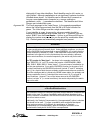
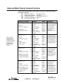
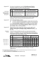
Steam and Water Property Region-Specific Functions
The chart below describes the region-specific functions for calculating
steam and water properties:
P3pt = Triple point pressure = 8.858914E-02 psia
T3pt = Triple point temp. = 32.018 °F
Function & Inputs
=LIQPT2…(P, T)
Liquid
(LIQ)
P=Pressure
(from P3pt to 15500 psia)
T=Temperature
(from T3pt°F to TSat °F)
=WETPQ2… (P, Q)
Saturated
Steam
(WET)
P=Pressure
(from P3pt to PCpt psia)
Q=Quality
(from 0% to 100%,
enter as 0 to 1)
=WETTQ2…(T, Q)
Note: The ratio of
specific heats is not
available under the
conditions described in
the appendix of the
Flow Measurement
chapter on page “FlowA4”.
T=Temperature
(from T3pt °F to TCpt °F)
Q= Quality
(from 0% to 100%,
enter as 0 to 1
=STMPT2…(P, T)
Superheated
Steam (STM)
P=Pressure
(from P3pt to PCpt psia)
T=Temperature
(from TSat °F to 1500 °F)
=CRTPT2…(P, T)
Supercritical
Steam (CRT)
P=Pressure
(from PCpt psia to
15500 psia)
T=Temperature
(from TCpt to 1500 °F)
R
Tsat = Saturation temperature = °F
PCpt = Critical point pressure = 3208.2347600665 psia
TCpt = Critical point temp.
= 705.47 °F
Result
Units
Example
…D
…H
…S
…C
…R
…V
…K
…U
Density
Enthalpy
Entropy
Specific Heat [Cp]
Ratio of Specific Heats
Specific Volume
Thermal Conductivity
Viscosity
Lb/Cuft
Btu/Lb
Btu/Lb°R
Btu/Lb°F
[Cp/Cv]
Cuft/Lb
Btu/Hr ft °F
Lb/Sec-ft
To obtain the enthalpy
of liquid at 2000 psia and
400°F, enter.
=LIQPTH(2000,400)
and your answer will be
377.1851 Btu/Lb.
…D
…H
…S
…T
…C
…R
…V
…K
…U
…D
…H
…S
…P
…C
…R
…V
…K
…U
Density
Enthalpy
Entropy
Temperature
Specific Heat [Cp]
Ratio of Specific Heats
Specific Volume
Thermal Conductivity
Viscosity
Density
Enthalpy
Entropy
Pressure
Specific Heat [Cp]
Ratio of Specific Heats
Specific Volume
Thermal Conductivity
Viscosity
Lb/Cuft
Btu/Lb
Btu/Lb°R
°F
Btu/Lb °F
[Cp/Cv]
Cuft/Lb
Btu/Hr ft °F
Lb/Sec-ft
Lb/Cuft
Btu/Lb
Btu/Lb °R
Psia
Btu/Lb °F
[Cp/Cv]
Cuft/Lb
Btu/Hr ft °F
Lb/Sec-ft
To obtain the entropy of
saturated steam at 1800
psia and 45% quality,
enter
=WETPQ2S(1800,.45)
and your answer will be
1.051466 Btu/Lb °R.
…D
…H
…S
…C
…R
…V
…K
…U
Density
Enthalpy
Entropy
Specific Heat [Cp]
Ratio of Specific Heat
Specific Volume
Thermal Conductivity
Viscosity
Lb/Cuft
Btu/Lb
Btu/Lb °R
Btu/Lb °F
[Cp/Cv]
Cuft/Lb
Btu/Hr ft °F
Lb/Sec-ft
To obtain the specific heat
of superheated steam at
2000 psia and 950 °F,
enter
=STMPT2C(2000,950)
and the result will be
0.652954 Btu/Lb °F.
…D
…H
…S
…C
…R
…V
…K
…U
Density
Enthalpy
Entropy
Specific Heat [Cp]
Ratio of Specific Heat
Specific Volume
Thermal Conductivity
Viscosity
Lb/Cuft
Btu/Lb
Btu/Lb °R
Btu/Lb °F
[Cp/Cv]
Cuft/Lb
Btu/Hr ft °F
Lb/Sec-ft
To obtain the thermal
conductivity of supercritical steam at 6000 psia
and 1200 °F, enter
=CRTPT2K(6000,1200)
to get 0.073924
Btu/Hr ft °F.
EndResult®
©2003 Sega Inc.
To obtain the specific
volume of saturated steam
at 200 °F and 70% quality,
enter.
=WETTQ2V(200,.7) and
the result will be 23.55216
Cuft/Lb.
EREXCEL-20
November 1, 2002 - English
Saturation Pressure & Temperature Functions
The chart below describes two functions which compute saturation
pressure and temperature:
P3pt
T3pt
PCpt
TCpt
TSat
= Triple point pressure
= Triple point temperature
= Critical point pressure
= Critical point temperature
= Saturation temperature
= 8.858914E-02 psia
= 32.018 °F
= 3208.2347600665 psia
= 705.47 °F
= °F
Function
Result
Example
=T2P(T)
Saturation
Pressure
To obtain the saturation pressure
of 79 °F steam, enter =T2P(79)
and the answer will be
0.490491psia
Saturation
Temperature
To obtain the saturation
temperature of 2000 psia steam,
enter =P2T(2000) and your answer
will be 635.8028 °F
T=Temperature
(from T3pt to TCpt °F)
=P2T(P)
P=Pressure
(from P3pt to PCpt psia)
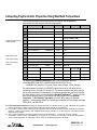
Steam and Water Property Examples Worksheet
Part of the STEAM.XLS worksheet from your EndResult® Examples disk
is shown below. The STEAM.XLS worksheet provides a working example
of all 79 steam and water property functions. You can experiment with
each function by entering numbers into the highlighted unprotected userinput cells. The minimum and maximum value for each input is displayed
just beneath each input cell. To compute steam density for example, cell
E16 contains the formula =ANYPT2D($B$16,$B$20). The remaining
results in column E are computed in a similar manner.
A
B
16
Press. =
5000
17
min:
18
max:
C
Psia
E
F
G
Density =
5.8210023
Lb/Cuft
=ANYPT2D(P,T)
0.08859
Enthalpy =
1529.1494
Btu/Lb
=ANYPT2H(P,T)
15500
Entropy =
1.5060786
Btu/Lb °R
=ANYPT2S(P,T)
Viscosity =
2.529E-05
Lb/Sec-ft
=ANYPT2U(P,T)
Spec. Vol. =
0.1717917
Cuft/Lb
=ANYPT2V(P,T)
Ther. Cond. =
0.0681597
19
20
Temp. =
1200
21
min:
32.018
22
max:
1500
23
R
D
EndResult®
°F
Btu/Hr ft °F =ANYPT2K(P,T)
Specific Heat [Cp] =
.7382281
Btu/Lb °F
=ANYPT2C(P,T)
Ratio of Specific Heats =
1.349910
[Cp/Cv]
=ANYPT2R(P,T)
©2003 Sega Inc.
EREXCEL-21
November 1, 2002 - English
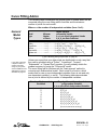
Boiler Efficiency Add-in
The boiler efficiency add-in contains functions which perform many of the
calculations necessary for computing boiler efficiency and gas turbine
performance including:
# Moisture per Lb of Dry Ambient Air
# Specific Heat of Air
# Specific Heat of Flue Gas
# Combustion Calculations
The boiler efficiency add-in provides added flexibility by allowing you to
either enter or compute many important quantities such as CO2, O2, H2O,
SO2, Excess Air, dry and wet gas constituents, and air heater leakage.
Many of the calculations performed by the boiler efficiency add-in are
based on equations found in Steam Generating Units31 Power Test Code
(PTC 4.1) and formulations found in Steam/Its Generation and Use32.
Individuals who are familiar with PTC 4.1 will find several of the example
worksheets to be self-explanatory.
Inputs and results which are the same as those on the PTC 4.1 short form
test such as ”ENTHALPY OF WATER ENTERING" are preceded by a number
followed by an equal’s sign (e.g. 17=Enthalpy of Water Entering) in both the
EndResult® example worksheets and the EndResult® Reference Manual.
The COMBCYC.XLS, COGEN3.XLS, GASTURB.XLS, GASTURBI.XLS, HTWUNIT.XLS,
PKGBLR.XLS, and UTILBLR.XLS worksheets (provided on your EndResult®
Pre-defined Spreadsheet Solutions disk) demonstrate how you can use the
calculations for combustion, moisture per pound of air, specific heat of air,
and specific heat of flue gas to compute boiler efficiency. The
COMBCYC.XLS, COGEN3.XLS, GASTURB.XLS, GASTURBI.XLS, HTWUNIT.XLS,
PKGBLR.XLS worksheets compute the combustion products of boilers and
gas turbines without an air heater, and the UTILBLR.XLS worksheet
computes the efficiency of a boiler with an air heater.
________________________
31 Steam Generating Units, Power Test Code (PTC) 4.1, (New York: American Society of Mechanical Engineers, 1974).
32 Babcock & Wilcox. Steam/Its Generation and Use, 40th Edition (New York: Babcock & Wilcox Company, 1992),
Section 6.
R
EndResult®
©2003 Sega Inc.
EREXCEL-22
November 1, 2002 - English
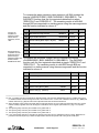
Moisture per Lb of Dry Ambient Air33
The moisture per pound of dry ambient air can be computed by the following
four methods using either relative humidity (Methods 1 & 2) or wet-bulb
temperature (Methods 3 & 4).
The fast, approximate, and simplest method to compute moisture per
pound of dry ambient air for a given relative humidity and pressure is to
use the function H2ONAIR (dry_bulb_temp, rel_humidity, air_pressure).
In the MOISTURE.XLS worksheet from your Examples disk (shown below),
cell. B4 contains the formula =H2ONAIR($B$1, $B$2, $B$3).
Method 1:
A
Default is 14.696 psia if "
pressure is omitted.
Method 2:
B
1
Ambient air dry-bulb temperature
2
Ambient air relative humidity
3
Ambient air pressure
4
Moisture per Lb of Dry Ambient Air
52
C
(from -80°°F to 200°°F)
65%
(from 0% to 100%, 0 to 1)
14.696
(from 2.25e-14 to 15.472 psia)
5.3115E-03
Lb/Lb
The slower but more rigorous method to compute moisture per pound of
dry ambient air (i.e. “Humidity Ratio”) for a given relative humidity and
pressure is to use the GAS2HMR function as described on page
“EREXCEL-15”.
The fast, approximate, and simplest method to compute moisture per
pound of dry ambient air for a given wet-bulb temperature34 and pressure
is to use the function H2ONAIRW (dry_bulb_temp, wet_bulb_temp,
air_pressure). In the MOISTURE.XLS worksheet from your Examples disk
(shown below), cell B9 contains the formula =H2ONAIRW($B$6, $B$7,
$B$8).
Method 3:
A
Default is 14.696 psia if
pressure is omitted. →
Method 4:
B
C
6
Ambient air dry-bulb temperature
65
(from -80°°F to 200°°F)
7
Ambient air wet-bulb temperature
58
(from 40.977°°F to 65°°F)
8
Ambient air pressure
14.696
(from 2.25e-14 to 15.472 psia)
9
Moisture per Lb of Dry Ambient Air
8.6698E-03
Lb/Lb
The slower but more rigorous method to compute moisture per pound of
dry ambient air (i.e. “Humidity Ratio”) for a given wet-bulb temperature34
and pressure is to use the GAS2HMR function as described on page
“EREXCEL-16”.
_______________________
33 For a graph of moisture per pound of dry ambient air, see the “ASHRAE Psychrometric Chart No. 1 (Normal
Temperature)” and “ASHRAE Psychrometric Chart No. 2 (Low Temperature)” in the appendix of the Boiler Efficiency
chapter.
34 The wet-bulb temperature cannot be greater than the dry-bulb temperature. To obtain the minimum wet-bulb
temperature, use the function =WETTEMP (dry_bulb_temp, 0, air_pressure). For example, if the dry-bulb temperature is
65°F and the air pressure is 14.696 psia, then the minimum wet-bulb temperature is 40.977°F.
R
EndResult®
©2003 Sega Inc.
EREXCEL-23
November 1, 2002 - English
Specific Heat of Air
The specific heat of air can be computed by the following two methods:
The fast, approximate, and simplest method to compute specific heat of
air at 14.696 psia is to use the function AIRT2C (air_temperature). In the
AIR-CP.XLS worksheet from you Examples disk (shown below), cell B3
contains the formula =AIRT2C($B$1). The AIRT2C function reproduces
the values given in Steam Generating Units35 Power Test Code (PTC
4.1), Figure 3. The AIRT2C function is convenient and provides adequate
accuracy in many situations.
Method 1:
A
1
B
Air temperature
400
C
(from 0°°F to 1000°°F)
2
3
Method 2:
Specific Heat of Air (=AIRT2C)
0.24498
Btu/Lb °F
The slow but more rigorous method to compute the specific heat of air at
any pressure is to use the mixed gas GAS2C function as described on
pages “EREXCEL-15” and “EREXCEL-16”.
Specific Heat of Flue Gas
The specific heat of flue gas can be computed by the following two methods:
The fast, approximate, and simplest method to compute specific heat of
flue gas at 14.696 psia is to use the function GASTR2C (gas_temp,
carbon_to_hydrogen_ratio). In the GAS-CP.XLS worksheet from you
Examples disk (shown below), cell B4 contains the formula
=GASTR2C($B$1,$B$2). The GASTR2C function reproduces the values
given in Steam Generating Units35 Power Test Code (PTC 4.1), Figure 7.
The GASTR2C function is convenient and provides adequate accuracy in
many situations.
Method 1:
A
B
C
(from 0°°F to 1000°°F)
1
Flue gas temperature
500
2
Carbon to Hydrogen Ratio
20
(from 0 to 100)
0.249725
Btu/Lb °F
3
4
Method 2:
Specific Heat of Flue Gas (=GASTR2C)
The slower but more rigorous method to compute the specific heat of flue
gas at any pressure is to use the mixed gas GAS2C function described on
page “EREXCEL-12”.
_________________________
35 Steam Generating Units, Power Test Code (PTC) 4.1, (New York: American Society of Mechanical Engineers, 1974).
R
EndResult®
©2003 Sega Inc.
EREXCEL-24
November 1, 2002 - English
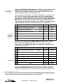
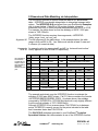
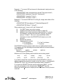
Combustion Calculations
The COMBUST.XLS worksheet from your Examples disk is shown below.
Each molar combustion function requires 12 input arguments. The name
of each argument appears in cells A1 to A17 and an example value for
each argument appears in cells B1 to B17. ASME numbers (where
applicable) appear in column A, and valid ranges for each input are listed
in column C.
The Flue gas Measurement
Selection pertains to the flue”
gas measurements shown on
rows 13 through 17 below. "
A
B
1
Flue Gas Measurement Selection
2
Air Heater Selection
Before
(either Before, After, or None)
3
43=Ultimate Analysis Carbon
49.8%
(from 0% to 100% by Weight)
4
44=Ultimate Analysis Hydrogen
3.5%
(from 0% to 100% by Weight)
5
45= Ultimate Analysis Oxygen
8.5%
(from 0% to 100% by Weight)
6
46=Ultimate Analysis Nitrogen
.7%
(from 0% to 100% by Weight)
7
47=Ultimate Analysis Sulfur
.6%
(from 0% to 100% by Weight)
8
37=Ultimate Analysis Moisture
30.4%
(from 0% to 100% by Weight)
9
22=Dry Refuse per Lb As Fired Fuel
0.0576
(from 0 to 1 Lb/Lb)
10
23=Btu per Lb in Refuse (Wtd. Avg.)
48.7
11
Moisture per Lb of Dry Ambient Air
6.6598E4
12
36=Percent Excess Air
Before air heater "
13
32 =Carbon Dioxide in Flue Gas Before AH
Before air heater "
14
33 =Oxygen in Flue Gas Before AH
Before air heater "
15
The Air Heater Selectioh
determines whether each
"
result described on pages 27
and 28 applies to conditions
before the air heater, after
the air heater, or to a boiler
without an air heater (None).
Argument #3 must be the
Ultimate Analysis Range. In "
this example, the ultimate
analysis is the shaded region
to the right.
Your fuel ultimate analysis "
ash is assumed by the add-in
to be 100% minus the total of
the specified ultimate
analysis constituents.
After air heater "
After air heater "
Dry
C
(either Wet or Dry)
(from 0 to 14500 Btu/Lb)
(from 0 to .081 Lb/Lb)
36
#N/A
(from -100% to 15000%, or #N/A)
37
#N/A
(from 0% to 20.9% by Vol, or #N/A)
37
3.5%
(from 0% to 20.9% by Vol, or #N/A)
34 =Carbon Monoxide in Flue Gas Before AH
37
.05%
(from 0% to 20.9% by Vol)
16
Diluted Carbon Dioxide after Air Heater
#N/A
(from 0% to 20.9% by Vol, or #N/A)
17
Diluted Oxygen after Air Heater
4%
(from 0% to 20.9% by Vol, or #N/A)
36
36
36
36
18
19
24=Carbon burned per Lb As Fired Fuel
.4978065
Lb/Lb
Each combustion calculation add-in function requires the same arguments
as the CARBURNED function in cell B19. To compute the Carbon burned
Notice that argument
per Lb as Fired Fuel, cell B19 contains the formula =CARBURNED($B$1,
"
#3 is a range.
$B$2,$B$3:$B$8,$B$9,$B$10,$B$11,$B$12,$B$13,$B$14,$B$15,$B$16,
$B$17).
_______________________
36 See table on page “EREXCEL-26” for explanation.
37 ASME number applicable only if Flue Gas Measurement Selection is Dry.
R
EndResult®
©2003 Sega Inc.
EREXCEL-25
November 1, 2002 - English
As shown in the table below, set the Flue Gas Measurement Selection
according to whether you want to enter each flue gas constituent’s
volumetric percent of a wet or dry flue gas sample.38
Argument #1
Arg
No.
A “Wet” flue gas
sample contains water
vapor whereas a “dry”
flue gas sample is
water vapor free.
13
14
15
16
17
If Flue Gas Measurement Selection
is “Dry”, enter the following:
If the Flue Gas Measurement Selection
is “Wet”, enter the following:
32=Carbon Dioxide in Dry Flue gas Before AH
33-Oxygen in Dry Flue Gas before air heater
34=Carbon Monoxide in Dry Flue Gas before AH
Diluted Dry Gas CO2 after air heater
Diluted Dry Gas Oxygen after air heater
Carbon Dioxide in Wet Flue Gas before AH
Oxygen in Wet Flue Gas before air heater
Carbon Monoxide in Wet Flue Gas before AH
Diluted Wet Gas CO2 after air heater
Diluted Wet Gas Oxygen after air heater
Note: The higher the percent H2 and H2O in the fuel analysis, the more difference there will be
between a wet-basis measurement and a dry-basis measurement. Generally, analyzers classified
as insitu (in the gas stream) provide wet-basis (moisture not condensed out of sample)
measurements. However, you will need to consult your analyzer manual to be sure.
Set the Air Heater Selection to None if:
Argument #2
(1)
(2)
you want to compute flue gas properties for a boiler without an air heater.
you want to compute flue gas properties for a boiler with an air heater and
are not interested in the performance (i.e. leakage, etc.) of the air heater.
Set the Air Heater Selection to Before to compute flue gas properties before
an existing air heater. Set the Air Heater Selection to After to compute flue
gas properties after an existing air heater.
Argument #3 must be a range which includes in exact order the fuel
ultimate analysis carbon, hydrogen, oxygen, nitrogen, sulfur, and
moisture. The range in the example on page "EREXCEL-25"is from cell
B3 to B8.
Argument #3
The table below displays the different ways in which you can enter measured percentages
(shown as “__%”) for arguments 12 to 17. Be sure to enter #N/A (rather than zero) for any not
measured value. Specifying any combination of measured inputs not shown in the table below will
cause the function to return an error message (i.e. “#N/A”). Be sure that any measurements taken
for arguments 13 through 15 are taken before the air heater.
Arguments
#7-#12
Arg
No.
Before air heater "
Before air heater "
Before air heater "
After air heater "
After air heater "
If the Air Heater
Selection is ‘None’
If the Air Heater Selection
is ‘Before’ or ‘After’
12
36=Percent Excess Air
#N/A
#N/A
#N/A
__%
#N/A
#N/A
#N/A
#N/A
13
3239=Carbon Dioxide in Flue Gas Before AH
__%
#N/A
__%
#N/A
__%
#N/A
__%
__%
14
3339=Oxygen in Flue Gas Before AH
__%
__%
#N/A
#N/A
#N/A
__%
__%
__%
15
3439=Carbon Monoxide in Flue Gas Before AH
__%
__%
__%
__%
__%
__%
__%
__%
16
Diluted Carbon Dioxide after air heater
#N/A
#N/A
#N/A
#N/A
__%
#N/A
__%
#N/A
17
Diluted Oxygen after air heater
#N/A
#N/A
#N/A
#N/A
#N/A
__%
#N/A
__%
An example of each of the 21 combustion calculation add-in functions
appears in rows 19 through 48 of the spreadsheet on the following pages.
Each function uses the inputs from rows 1 through 17 on page
“EREXCEL-25”.
______________________
38 For instructions on “Converting a Wet-Basis Sample to a Dry-Basis Sample” using the “Mixed Gas Thermo-Physical
Properties” application see page “MixGas-12”.
39 ASME number applicable only if Flue Gas Measurement Selection is Dry.
R
EndResult®
©2003 Sega Inc.
EREXCEL-26
November 1, 2002 - English
To compute the Carbon burned per Lb As Fired Fuel, cell B19 contains the
formula =CARBURNED($B$1,$B$2,$B$3:$B$8,$B$9,$B$10,$B$11,
$B$12,$B$13,$B$14,$B$15,$B$16,$B$17). The results in cells B20
through B28 are computed in a similar manner using the same
arguments.40
A
Notice the placement of
the braces. "
B
C
19
24=Carbon burned per Lb As Fired Fuel
CARBURNED
.4978065
Lb/Lb
20
Dry Air per Lb As Fired Fuel (AFF)
DRYAIR
7.8629727
Lb/Lb
21
36=Percent Excess Air
EXCESSAIR
19.3790%
Percent
22
25=Dry Gas per Lb As Fired Fuel (ASME)
DRYGAS
8.1818799
Lb/Lb
23
Wet Air per Lb As Fired Fuel (AFF)
WETAIR
7.8682093
Lb/Lb
24
Dry Gas Including Fly Ash (Wt. Basis)
BALDRY
8.1885761
Lb/Lb
25
Dry Gas Excluding Fly Ash (Wt. Basis)
MOLEDRY
8.1811761
Lb/Lb
26
Wet Flue Gas Including Fly Ash (Wt. Basis)
WETGAS
8.8106093
Lb/Lb
27
Wet Flue Gas Excluding Fly Ash (Wt. Basis)
MOLEWET
8.8032093
Lb/Lb
28
Air Heater Leakage (Actual)
LEAKAGE
2.57876%
% by Wt.
Likewise, Carbon Burned per Lb As Fired Fuel (in cell B19) could also be
computed by entering each argument directly as in:
=CARBURNED("Dry","Before",{.498,.035,.085,.007,.006,.304},0.0576,
48.7,6.65979E-04,#N/A,#N/A,.035,.0005,#N/A,.04).
The dry flue gas constituents in cells B30 through B33 are computed by
the ASME method which assumes that SO2 condenses out with H2O. To
compute the carbon dioxide in dry flue gas by the ASME method, cell B30
contains the formula =DRYCO2($B$1,$B$2,$B$3:$B$8,$B$9,$B$10,
$B$11,$B$12,$B$13,$B$14,$B$15,$B$16,$B$17). The remaining dry
flue gas constituents in cells B31 through B33 are also computed by the
ASME method using the same arguments.
A
B
C
30
32=Carbon Dioxide (CO2) in Dry Flue Gas (ASME)
DRYCO2
15.54476%
% by Vol
31
33=Oxygen (O2) in Dry Flue Gas (ASME)
DRYO2
3.50000%
% by Vol
32
34=Carbon Monoxide in Dry Flue Gas (ASME)
DRYCO
0.05000%
% by Vol
33
35=Nitrogen (N2) in Dry Flue Gas (ASME)
DRYN2ASME
80.90524%
% by Vol
100.00000%
% by Vol
34
Total
______________________
40 Hint: To quickly enter the cell formulas in cells B20 to B28, enter the entire CARBURNED function in cell B19, then copy
it to cells B20 to B28, and then change each cell to the correct function. Correct use of absolute references (e.g. $B$2)
and relative references (e.g. B2) will ensure that copied formulas have the desired references.
R
EndResult®
©2003 Sega Inc.
EREXCEL-27
November 1, 2002 - English
Notice the
placement of the
braces.
Likewise, Carbon Dioxide in Dry Flue Gas (in cell B30 on the preceding page)
" could also be computed by entering each argument directly as in:
=DRYCO2("Dry","Before",{.498,.035,.085,.007,.006,.304},0.0576,48.7,
6.65979E-04,#N/A,#N/A,.035,.0005,#N/A,.04).
The dry flue gas constituents in cells B36 through B40 are computed by
the “Total Gas” method which assumes that SO2 is not condensed out
with H2O. To compute the carbon dioxide in dry flue gas by the “Total
Gas” method, cell B36 contains the formula =DRYCO2($B$1,$B$2,$B$3:
$B$8,$B$9,$B$10,$B$11,$B$12,$B$13,$B$14,$B$15,$B$16,$B$17).
The remaining dry flue gas constitutents in cells B37 through B40 are also
computed by the “Total Gas” method using the same arguments.41
A
Note: The add-in
assumes that 100%
of the sulfur is →
burned to yield
only SO2.
B
C
36
32=Carbon Dioxide (CO2) in Dry Flue Gas
DRYCO2
15.54476%
% by Vol
37
33=Oxygen (O2) in Dry Flue Gas
DRYO2
3.50000%
% by Vol
38
34=Carbon Monoxide in Dry Flue Gas
DRYCO
0.05000%
% by Vol
39
35=Nitrogen (N2) in Dry Flue Gas
DRYN2
80.83483%
% by Vol
40
Sulfur Dioxide (SO2) in Dry Flue Gas
DRYSO2
0.07041%
% by Vol
100.00000%
% by Vol
41
Total
To compute the carbon dioxide in wet flue gas, cell B43 contains the
formula =WETCO2($B$1,$B$2,$B$3:$B$8,$B$9,$B$10,$B$11,$B$12,
$B$13,$B$14,$B$15,$B$16,$B$17). The remaining wet flue gas
constituents in cells B44 through B48 are computed in a similar manner
using the same arguments.
A
(See note above) →
B
C
43
Carbon Dioxide (CO2) in Wet Flue Gas
WETCO2
13.75737%
% by Vol
44
Oxygen (O2) in Wet Flue Gas
WETO2
3.09756%
% by Vol
45
Carbon Monoxide (CO) in Wet Flue Gas
WETCO
0.04425%
% by Vol
46
Nitrogen (N2) in Wet Flue Gas
WETN2
71.54016%
% by Vol
47
Water Vapor (H2O) in Wet Flue Gas
WETH2O
11.49835%
% by Vol
48
Sulfur Dioxide (SO2) in Wet Flue Gas
WETSO2
.06231%
% by Vol
100.00000%
% by Vol
49
Total
Likewise, Carbon Dioxide in Wet Flue Gas (in cell B43) could also be computed by
entering each argument directly as in: =WETCO2,(“Dry”,”Before”,{.498,.035,
.085,.007,.006,.304},0.0576,48.7,6.65979E-04,#N/A,#N/A,.035,.0005,#N/A,.04).
______________________
41 Hint: To quickly enter the cell formulas in cells B37 to B40, enter the entire DRYCO2 function in cell B36, then copy it to
cells B37 to B40, and then change each cell to the correct function. Correct use of absolute references (e.g. $B$2) and
relative references (e.g. B2) will ensure that copied formulas have the desired references.
R
EndResult®
©2003 Sega Inc.
EREXCEL-28
November 1, 2002 - English
Heat Loss Due to Radiation
The RADLOSS and RADLOSS2 functions described in this section provide
two separate methods for computing ABMA radiation loss in percent as
fired fuel (%AFF) for a boiler. 69=Heat Loss Due To Radiation is the percent
of heat energy in the fuel lost to surface radiation and convection off the
outside skin of the boiler. Heat Loss Due to Radiation increases as: (1) the
Number of Water Walls (i.e. water-cooled furnace walls) decreases, (2) the
Air Velocity Around Boiler increases, and (3) the Air to Boiler Temperature Delta
(i.e. difference) increases.
The RADLOSS.XLS worksheet from your Examples disk is shown below. The
inputs appear in the first 12 rows, and the result appears in row 14. Cell
B14 contains the formula RADLOSS($B$1,$B$2,$B$3,$B$4,$B$5,$B$6,
$B$7,$B$8,$B$9,$B$10,$B$11,$B$12). ASME numbers (where
applicable) appear in column A, and valid ranges for each input are listed
in column C.
A
For standard radiation
loss enter an air
velocity around boiler
of 100 FPM and an air
to boiler temperature
delta of 50°F.
If the boiler does not
have a reheater, enter
#N/A for the last three
arguments
(i.e. cells B10 to B12).
B
4800000
C
1
Boiler Capacity
2
Number of Water Walls
3
Drum Blowdown Water Flow
4
Air Velocity Around Boiler
100
(from 0 to 1800 FPM)
5
Air to Boiler Temperature Delta
50
(from 0°°F to 2000°°F)
6
15=Enthalpy of Saturated Liquid
733.5924
(from 1E-7 to 906.96 Btu/Lb)
7
16=Enthalpy of Superheated Steam
1460.3950
(from 715.86 to 1586 Btu/Lb)
8
17=Enthalpy of Water Entering
442.5746
(from 1E-7 to 906.96 Btu/Lb)
9
26=Actual Water Evaporated
4640000
(from 500 to 10E+06 Lb/Hr)
10
18=Enthalpy of Steam at R.H. Inlet
1299.7101
(from 715.86 to 1586 Btu/Lb, or #N/A)
11
19=Enthalpy of Steam at R.H. Outlet
1520.2431
(from 715.86 to 1586 Btu/Lb, or #N/A)
12
27=Reheat Steam Flow
4
46000
4200000
(from 500 to 10E+06 Lb/Hr)
(from 0 to 4)
(from 0 to 10E+06 Lb/Hr)
(from 500 to 10E+06 Lb/Hr, or #N/A)
13
14
69=Heat Loss Due to Radiation RADLOSS
0.172002%
% AFF of gross heat input
You can also enter the formula values directly. For example, the radiation
loss shown in cell B14 above could also be calculated by entering the
formula =RADLOSS(4800000,4,46000,100,50,733.5924,1460.3950,
442.5746,4640000,1299.7101,1520.2431,4200000).
R
EndResult®
©2003 Sega Inc.
EREXCEL-29
November 1, 2002 - English
Although RADLOSS is not compensated for superheat or reheat spray flow,
because of the nature of radiation loss on large boilers, the error is
considered negligible. However, if you prefer you can calculate the
maximum boiler heat output and the actual heat output and use
RADLOSS2.
The PKGBLR.XLS and UTILBLR.XLS worksheets (provided on your
EndResult® Pre-defined Spreadsheet Solutions disk) demonstrate how the
radiation loss (RADLOSS) add-in function can be combined with other
functions to compute boiler efficiency. The PKGBLR.XLS worksheet
computes the efficiency of a boiler without a reheater, and the UTILBLR.XLS
worksheet provides a demonstration of an efficiency calculation for a
boiler with a reheater.
The RADLOSS2.XLS worksheet from your EndResult® Examples disk is
shown below. The inputs appear in the first 5 rows, and the result
appears in row 7. Cell B7 contains the formula
=RADLOSS2($B$1,$B$2,$B$3,$B$4,$B$5). ASME numbers (where
applicable) appear in column A, and valid ranges for each input are listed
in column C.
A
The Actual Btu cannot be
greater than the rated
Btu.
For standard radiation
loss enter an air velocity
around boiler for 100 FPM
and an Air to Boiler
Temperature Delta of
50°F.
B
C
1
Actual Btu
200
(from 1 to 10E+06 Mbtu/Hr)
2
Rated Btu
400
(from 1 to 10E+06 Mbtu/Hr)
3
Number of Water Walls
4
Air Velocity Around Boiler
100
(from 0 to 1800 Fpm)
5
Air to Boiler Temperature Delta
50
(from 0°°F to 2000°°F)
4
(from 0 to 4)
6
7
69=Heat Loss Due to Radiation
RADLOSS2
0.61718%
% AFF of gross heat input
Likewise, Heat Loss Due to Radiation (in cell B7) can also be computed by
entering each argument directly as in: =RADLOSS2(200,400,4,100,50).
The HTWUNIT.XLS worksheet (provided on your EndResult® Pre-defined
Spreadsheet Solutions disk) demonstrates how the radiation loss
(RADLOSS2) add-in function can be combined with other functions to
compute boiler efficiency.
R
EndResult®
©2003 Sega Inc.
EREXCEL-30
November 1, 2002 - English
Curve Fitting Add-in
The following table summarizes the general types of models which can be
computed using the curve fitting add-in functions and the minimum
number of points for each model.
Where n = the number of independent variables (from 1 to 9):
General Equation
Model
Minimum
y=Dependent Variable
Type
Number
x1,x2,x3,etc.=Each Independent Variable
of Points
A1,A2,A3,etc.=Each Coefficient
Polynomial...............depends(*).........y = A1(x1)n + A2(x2)n + ... + const
Power .......................... n + 1..............y = (x1)A1 * (x2)A2 * ... * (xn)An * An+1
Logarithmic.................. n + 1..............y = A1LN(x1) + A2LN(x2) + ... + AnLN(xn) + An+1
Inverse......................... n + 1..............y = A1/x1 + A2/x2 + ... + An/xn + An+1
Exponential.................. n + 1..............y = e^(A1x1) * e^(A2x2) * ... * e^(Anxn) * An+1
Square root.................. n + 1..............y = A1(x1)(1/2) + A2(x2)(1/2) + ... + An(xn)(1/2) + An+1
General
Model
Types
(*) See "Modeling Using Polynomials" on page 36.
Unless you expect that your data points are distributed in such a way that
they can be modeled using a "Power", "Logarithmic", "Inverse",
"Exponential", or "Square Root" equation, you will probably obtain the
greatest accuracy by using the "Polynomial" model.
The curve fitting add-in functions use the "least squares" method to
compute each mathematical model. Each model is a function, which
means that for one or more independent variables, there is one and only
one dependent variable (i.e. result). The following table demonstrates
how a point is defined by the number of independent variables:
If you want to develop
a square model or a
square root model
using only two points,
see the SQRXYXY and
SQRTXYXY functions
described on page 47.
Number of Independent
Variables
1
2
3
4
5
6
7
8
9
R
EndResult®
Required format for each point
y=Dependent Variable
x1,x2,x3,etc.=Each Independent Variable
(x1,y)
(x1,x2,y)
(x1,x2,x3,y)
(x1,x2,x3,x4,y)
(x1,x2,x3,x4,x5,y)
(x1,x2,x3,x4,x5,x6,y)
(x1,x2,x3,x4,x5,x6,x7,y)
(x1,x2,x3,x4,x5,x6,x7,x8,y)
(x1,x2,x3,x4,x5,x6,x7,x8,x9,y)
©2003 Sega Inc.
EREXCEL-31
November 1, 2002 - English
Curve Fitting Add-in Functions
The chart below summarizes the curve fitting add-in functions.
FITEQ (cont.)
select Edit Paste Special…, (3) Click the Values
option button and then click OK, and (4) Insert an
equals sign (“=”) at the beginning of the equation.
=FITEQ (point_range, type$)
=FITVAL (point_range, type$, IV$)
=FITR2 (point_range, type$)
=FITAVGDEV (point_range, type$)
=FITMAXDEV (point_range, type$)
=EQFRAGMENT (point_range, type$, fragment)
type$ = the model type (enclosed in quotes) must be
selected from the following list:
“sqrt” for a square root model,
“log” for a logarithmic model,
“inv” for an inverse model,
“power” for a power model,
“exp” for an exponential model, or
“poly n” for an nth degree polynomial
where n is from 1 to 9.
See “Taking the nth Derivative of a Model” on page
36 for additional options which you can include in
your type$.
Since there is no reason
to compare your original
points to a derivative of
your model, the FITR2,
FITAVGDEV, and
FITMAXDEV
functions will return
“#N/A” if you have "
any “d/” instructions
in your model type$.
point_range = a range containing from 2 to 150 data
points. As shown in the example on the following
page, the first row of the point_range should contain
the name of each independent variable and the
name of the dependent variable. You can specify
from 1 to 9 independent variables. You should
provide a separate column for each independent
variable. However, the rightmost column should
always contain the dependent variable. The data
points in the example worksheet on the following
page contain only one independent variable “X” and
the dependent variable “Y”.
We recommend that you
allocate a named cell in
your worksheet to store
the value of each
independent variable.
You can assign a name
to a cell by selecting
Insert Name Define…
from the Microsoft®
Excel (Versions 3, 4, or
7) menus or Formula
Define Name… from the
Microsoft® Excel
(Version 5) menu. For
example, the
independent variable X
was defined as cell $E$2
shown on page 33.
IV$ = the value of each independent variable enclosed in
quotes (e.g. “press=6.31, temp=7.31”). Each
independent variable name must appear in the top
row of the point_range in all but the rightmost
column.
fragment = the nth part of an equation. The beginning of
the equation is always fragment 1.
FITEQ returns the equation of the type$ model which fits
the data in the spreadsheet. FITEQ uses the
independent and dependent variable names which
you specified in the first row of your point_range.
Cell C23 on the following page contains the formula
=FITEQ($A$1:$B$19,”Poly2”) which returns the
equation of the 2nd-order polynomial which fits the
data points in the point_range. To obtain a “live”
function: (1) Select Edit Copy…, (2) Move the
pointer to a different cell and
R
EndResult®
©2003 Sega Inc.
FITVAL returns the value of the type$ model for the given
values of the independent variables. Cell E35 on
page 34 contains the formula
FITVAL($A$1:$B$19,"exp","x=72") which returns the
value of the exponential model at x = 72. The
=FITVAL function should only be used for “spot
checking”. Once your model is finished, be sure to
use the FITEQ function to convert the model to a
“live” equation.
FITR2 returns the correlation coefficient (r2) of the type$
model. The value of r2 is from 0 to 1, and the closer
r2 is to 1, the better the fit. A correlation coefficient
of 1 is a perfect fit. Cell D36 on page 34 contains
the formula =FITR2($A$1:$B$19,"sqrt") which
returns the correlation coefficient of the square root
curve which fits the data points in the point_range.
FITAVGDEV returns the average absolute deviation of
the type$ model from the specified points. The
average absolute deviation is the average gap (or
average error) between the model and the entered
points. If the computed model passes directly
through all of the entered points, the average
absolute deviation will be zero. Cell C37 on page
34 contains the formula
=FITAVGDEV($A$1:$B$19,"log") which returns the
average absolute deviation of the logarithmic
equation from the data points in the point_range.
FITMAXDEV returns the maximum absolute deviation
(i.e. maximum error) of the type$ model from
specified points. The maximum absolute deviation
is the largest gap (or greatest error) between the
model and any of the entered points. If the
computed model passes directly through all of the
entered points, the maximum absolute deviation will
be zero. Cell B38 on page 34 contains the formula
=FITMAXDEV($A$1:$B$19,"power") which returns
the maximum absolute deviation of the power
equation from the data points in the point_range.
EQFRAGMENT is discussed in the section entitled
“Computing Equations Longer than 255 Characters”
on page 41.
EREXCEL-32
November 1, 2002 - English
Part of the FIT.XLS worksheet from your EndResult® Examples disk is shown below:
A
Note: To sort your points
in either ascending or
descending order, select
the entire table of points
and use the Data Sort…
command.
"
B
1
X
Y
2
15.93
0.850
3
18.79
4.410
4
19.99
8.710
5
24.70
9.31
6
31.86
14.62
7
34.12
17.32
8
34.35
17.58
9
38.40
21.08
10
45.36
23.94
11
52.44
25.87
12
55.83
37.11
13
59.64
40.13
14
61.31
45.89
15
63.24
49.66
16
68.08
56.89
17
68.19
57.69
18
70.88
60.49
19
74.73
65.05
C
D
E
X=
72
F
20
R
21
Model Type
Equation returned by FITEQ
22
Polynomial (1st)
Y=
23
Polynomial (2nd)
Y=
+1.48114956107175+0.00676722952131612*X+0.0115013843515338*X^2
24
Exponential
Y=
+2.00069041435995*EXP(0.0507535135189556*X)
25
Square Root
Y=
-56.7239732569892+13.164884868393*X^0.5
26
Logarithmic
Y=
-116.206639541582+39.3830687552381*LN(X)
27
Power
Y=
+0.00825314588685043*X^2.10208656290306
28
Inverse
Y=
+63.2729139063545-1195.43012344389/X
EndResult®
-17.7142520110828+1.04489704024574*X
©2003 Sega Inc.
EREXCEL-33
November 1, 2002 - English
The data points and equations from the previous page are shown on the
graph below:
Exponential Fit
100
Power Fit
2nd Degree Polynomial Fit
1st Degree Polynomial Fit
Square Root Fit
Logarithmic Fit
50
Inverse Fit
Y
0
-50
5
37
21
53
69
85
X
A
B
C
D
E
F
30
Model
Maximum
Average
Correlation
Value at
31
Type
Deviation
Deviation
Coefficient
X=72
=FITMAXDEV
=FITAVGDEV
=FITR2
=FITVAL
29
32
R
st
33
Polynomial (1 )
11.2101
3.2109
0.959092
57.5183
34
Polynomial
nd
(2 )
7.5943
2.0504
0.984010
61.5916
35
Exponential
23.7425
5.2464
0.923115
77.3040
36
Square Root
12.7402
4.7785
0.925357
54.9838
37
Logarithmic
13.8673
6.3737
0.875620
52.2216
38
Power
8.1316
2.9507
0.976033
66.2054
39
Inverse
17.7737
9.4447
0.739488
46.6697
EndResult®
©2003 Sega Inc.
EREXCEL-34
November 1, 2002 - English
Modeling Using Polynomials
The following table lists the minimum number of points which you must
enter to compute polynomial equations of various degrees with various
numbers of independent variables.
1
2
3
4
5
6
7
8
9
Maximum
Polynomial
Degree
1
2
3
4
5
6
7
8
9
10
9
2
3
6
10
15
2
28
36
45
--
8
3
4
10
20
35
--
--
--
--
--
4
4
5
15
35
--
--
--
--
--
--
3
5
6
21
--
--
--
--
--
--
--
2
6
7
28
--
--
--
--
--
--
--
2
7
8
36
--
--
--
--
--
--
--
2
8
9
45
--
--
--
--
--
--
--
2
9
10
--
--
--
--
--
--
--
--
1
Minimum
Number
of Points
Number
of Independent
Variables
Polynomial Degree
Additionally, the rightmost column of the table above shows the maximum
degree polynomial which can be computed by the curve fitting add-in
functions due to the number of independent variables.
The following table contains several commonly used polynomial models
which can be computed using the curve fitting add-in functions.
Form of
Polynomial
Model
Type$
Number of Minimum
Independent Number
Variables
of Points
(1 to 9)
Polynomial Equations
(*)
y=Dependent Variable
Polynomial
x1x2x3,etc.=Each Independent Variable Degree
A,B,C,etc.=Each Coefficient
(1 to 9)
Linear .........................."Poly1"................... 1.......................2 .................y = Ax1 + B...............................................................1
Parabolic ....................."Poly2"................... 1.......................3 .................y = A(x1)2 + B(x1) + C ...............................................2
Cubic ..........................."Poly3"................... 1.......................4 .................y = A(x1)3 + B(x1)2 + C(x1) + D..................................3
Quartic........................."Poly4"................... 1.......................5 .................y = A(x1)4 + B(x1)3 + C(x1)2 + D(x1) + E.....................4
Plane ..........................."Poly1"................... 2.......................3 .................y = A(x1) + B(x2) + C ................................................1
Paraboloid(*) ..............."Poly2"................... 2.......................6 .................y = A(x1)2 + B(x1) +C(x2)2 + D(x2) + E(x1)(x2) + F......2
(* eliptic or hyperbolic)
Large Polynomial ........"Poly2"................... 3......................10 ................y = A(x1)2 + B(x2)2 + C(x3)2 + D(x1) + E(x2) ...............2
.................................................................... ......................... .................. + F(x3) + G(x1)(x2) + H(x1)(x3) + I(x2)(x3) + J
First Degree ................... NA ...................... n....................n + 1 ..............y = A1x1 + A2x2 + ... + Anxn + An+1 ........................... NA
(*) In the polynomial equations above, the highest power of an
independent variable (e.g. X1, X2, X3, etc.) in the equation is the
“Polynomial Degree” shown in the rightmost column.
R
EndResult®
©2003 Sega Inc.
EREXCEL-35
November 1, 2002 - English
You should probably experiment with many different degrees of
polynomial fits, before deciding which polynomial model is the best.
Typically, there is an optimum degree of fit for the polynomial. Computing
for degrees which are higher or lower than the optimum degree may
decrease the desirability or accuracy of the fit.
The example graph below illustrates how a curve fit with a lower degree
(and a lower correlation coefficient) may be a more suitable model for the
data than a curve fit with a higher degree (and a higher correlation
coefficient).
This curve fit has a has a higher
correlation coefficient but does not
provide a suitable model of the data.
100
This curve fit has a lower correlation
coefficient but provides a more
suitable model of the data.
y
0
x
0
100
Taking the nth Derivative of a Model
The table below demonstrates how you can take the nth derivative of a
model by adding one or more “d/” instructions to your model type$ (type$
is discussed on page 32). If you have multiple independent variables in
your model, then you can obtain the nth partial derivative with respect to
one or more independent variable(s).
Example Formulas
Examples Explained
=FITEQ($A$1:$B$19,"Poly4 d/X^2”)
Computes the equation of the 2nd
derivative with respect to X of the
4th degree polynomial.
=FITVAL($A$1:$B$19,"Poly5 d/A^2
d/B","A=3,B-5")
Computes the value of the 2nd
derivative with respect to A and the
1st derivative with respect to B of
the 5th degree polynomial at the
value A=3 and B=5.
=FITEQ($A$1:$B$19, “Poly4 d/X d/X”)
Computes the equation of the 2nd
derivative with respect to X of the
4th degree polynomial.
Since there is no reason to compare your original points to a derivative of
your model, the FITR2, FITAVGDEV, and FITMAXDEV functions will
return “#N/A” if you have any “d/” instructions in your model type$.
R
EndResult®
©2003 Sega Inc.
EREXCEL-36
November 1, 2002 - English
Determining the Accuracy of the Fit
Each model computed by the curve fitting add-in functions is a “best
fitting” curve which passes directly through or as close to the entered
points as possible with a smooth transition between the points. As you
might expect, if your data is “scattered,” it may be difficult to find a curve
which closely fits all of your points. The maximum (FITMAXDEV) and
average (FITAVGDEV) deviations, as well as the correlation coefficient
(FITR2), provide a measure of accuracy of each type of fit to the points.
The best fitting model has the smallest maximum and average deviations
and the largest correlation coefficient. However, since even curves with a
good fit can include unexpected or undesirable changes in direction, you
should always graph your data along with each computed model to
determine which curve fit is most appropriate, applicable, and realistic for
your particular situation.
Developing Accurate Models
You want to have as many data points as possible when developing an
accurate model. You should experiment with several different types of
models to determine which model fits your data most appropriately. The
best way to do this kind of experimentation is by plotting each model on a
graph. For example, if you are using a mathematical model for
forecasting, (i.e., to predict values beyond the points which you currently
know), then you should test how different types of models react in the
forecasted range by plotting each one on a graph. The example graph on
page 34 demonstrates how your computed results depend greatly on
which type of model you choose.
R
EndResult®
©2003 Sega Inc.
EREXCEL-37
November 1, 2002 - English
Improving Accuracy by Modeling Small Regions Separately
If your data points are scattered, you may not be able to obtain a single
equation which will fit all of the points with the desired accuracy. In this
case, greater accuracy can be obtained by dividing your points into two or
more groups and then modeling each group separately. After you have
divided your points, you can make the transition between adjacent models
smoother by forcing the models to overlap. You can overlap adjacent
models by putting points on both sides of the model border into each
model’s point_range. (The point_range is discussed on page 32).
You can use the following procedure to determine when and where you
should use multiple models:
Step 1: Select a model type (e.g., “Poly3”, “Poly4”, etc.) which will
provide the best fit for all of the data points.
Step 2: Use this model to compute the dependent variable for each of
your known points.
Step 3: Compute the difference between the actual and computed
values of the dependent variable for each of your known points.
Step 4: If the model deviates significantly from some of the points, you
may need to take these points out of the main group and model
them separately.
Performing Linear Interpolation and Extrapolation
To perform linear interpolation or extrapolation, simply use the
FITEQ(point_range, “Poly1”) function (on page 32) to solve for a first
degree polynomial. After using the FITEQ function to compute the
equation of the line, you can compute points: (1) between your known
points (i.e., “interpolation”), or (2) beyond your known points (i.e.,
“extrapolation”).
If you want to perform interpolation or extrapolation using only two points,
see the INTERP and EXTRAP functions described on page 46.
R
EndResult®
©2003 Sega Inc.
EREXCEL-38
November 1, 2002 - English
Computing Equations Longer than 255 Characters
The longest equation which can be returned by the FITEQ function is 255
characters. To obtain an equation which is longer than 255 characters,
you must use multiple EQFRAGMENT functions. If the equation is too
long for FITEQ to display, it will return an “EQFRAGMENT” line like that
shown below:
Notice that this
“EQFRAGMEMT” line
indicates that the
→
equation is composed of
three fragments.
A
51
B
C
D
E
F
=EQFRAGMENT(point_range,"Poly6:,1)+…+EQFRAGMENT(point_range,"Poly6,3)
To return the entire function, you must enter each EQFRAGMENT
function into a separate cell as shown in cells B53 through B55 below.
Remember to replace
“point_range” with the
→
worksheet range
where your points
→
are located. For
example, the point range
→
for the points
on page 33 is
$A$1:$B$19.
A
B
C
D
53
=EQFRAGMENT(point_range,"Poly",1)
54
=EQFRAGMENT(point_range,"Poly6",2)
55
=EQFRAGMENT(point_range,"Poly6",3)
E
F
To convert each EQFRAGMENT function to a “live” equation:
(1) Select the cells containing the EQFRAGMENT functions,
(2) Select Edit Copy… from the Excel menu,
(3) Move the pointer to an empty area in the worksheet and Edit Paste Special…, and
(4) Click the Values option button and then click OK.
A
The long equation to the →
right was computed by fitting
th
a 6 –degree polynomial to→
the 100 points shown on the
graph on page 39.
→
B
C
D
E
F
57
+17.8371375215022+53.0912733397568*X-59.5706026033222*X^2+26.9864238073324…
58
+1.37678894596316*X^2*Y+0.770994294857225*Y^4-3.55348562565369*X*Y^3-…
59
+0.00381625498017175*Y^6-0.00587521503621247*X*Y^5-0.00655490897641504*X^2*…
60
=SUM(B57:B59)
Lastly, use a SUM() function to add up each of the fragments to determine
the value of the complete equation.
R
EndResult®
©2003 Sega Inc.
EREXCEL-39
November 1, 2002 - English
1-Dimensional Data Modeling via Polynomials
The chart below describes the functions for computing a best fitting least
squares polynomial curve to a set of data points.
Where y = anxn +…+ a2x2 + a1x + a0
=POLYSTR(x1:x99,y1:y99,n,x$)
=POLYVAL(x1:x99,y1:y99,n,x)
=POLYINDEX(x1:x99,y1:y99,n)
x1:x99,y1:y99=Independent and dependent
data point ranges which specify from 2
to 99 data points (x1,y1), (x2,y2),
(x3,y3),…, (xm,ym). Each range can be
either a single row or single column of
numbers. In the spreadsheet below,
the independent (x) range is from cell
A1 to A5, and the dependent (y) range
is from cell B1 to B5.
n = the degree of the computed polynomial
equation (from 1 to 8). However, if m
is the number of (x,y) points and n≥m,
the function will compute a polynomial
of degree m-1.
x = the value of the independent variable.
x$ = the cell address (enclosed in quotes)
of the independent variable such as
"$E$1".
POLYSTR returns the equation of an nth-degree
polynomial which fits the data in the spreadsheet.
Cell B7 below contains the formula
=POLYSTR($A$1:$A$5,$B$1:$B$5,2,"$E$1") which
returns a string representation of the equation of the
2nd-order polynomial which best fits the data in the
spreadsheet. To obtain a “live” function: (1) Select
Edit Copy…, (2) Move the pointer to a different cell
and select Edit Paste Special…, (3) Click the Values
option button and then click OK, and (4) Insert an
equals sign ("=") at the beginning of the equation.
POLYVAL returns the value of an nth-degree polynomial
which best fits the data in the spreadsheet for the
given value of x. Cell B8 below contains the formula
=POLYVAL($A$1:$A$5,$B$1:$B$5,2,72) which
returns the value of the 2nd degree polynomial which
fits the data in the spreadsheet where x = 72.
POLYINDEX returns the index of an nth-degree leastsquares polynomial of the specified degree. Cell B9
below contains the formula
=POLYINDEX($A$1:$A$5,$B$1:$B$5,2) which
returns the index of the 2nd-order polynomial equation
which fits the points in the spreadsheet. An index of 1
is a perfect fit. 42
The POLY.XLS worksheet from your EndResult® Examples disk is shown
below.
Note: To sort your (x,y)
points so that the x values
are in either ascending or
descending order, select
the table of (x,y) points and
use the Data Sort…
command.
→
A
B
C
1
20
81.9
2
40
83.1
3
60
84
4
80
84.6325
5
100
85.0302
D
E
X=
72
F
6
=POLYSTR→
7
y=
=POLYVAL→
8
y=
84.41942
9
index =
.999933
=POLYINDEX→
-3.3430357E-4*$E$1^2+0.0790809*$E$1+80.4586200
_______________________
42 For a discussion of the potential problems of trying to obtain a perfect fit see page “Curve-17” and “Curve-18”.
R
EndResult®
©2003 Sega Inc.
EREXCEL-40
November 1, 2002 - English
1-Dimensional Data Modeling via Derivatives
The chart below describes the functions for computing the first derivative of a
least squares polynomial which is fit to a set of data points.
Where y’ = an-1x n-1 + … + a2x2+a1x + a0
=DERIVSTR (x1:x99,y1:y99,n,x$)
=DERIVVAL (x1:x99,y1:y99,n,x)
=DERIVINDEX 1
x1:x99,y1:y99=Independent and dependent
data point ranges which specify from 2
to 99 data points (x1,y1), (x2,y2),
(x3,y3),…, (xm,ym). Each range can be
either a single row or single column of
numbers. In the spreadsheet below,
the independent (x) range is from cell
A1 to A5, and the dependent (y) range
is from cell B1 to B5.
n = the degree of the computed polynomial
from which the derivative is taken (from
1 to 8). However, if m is the number of
(x,y) points and n≥m, the function will
compute a polynomial of degree m-1.
x = the value of the independent variable.
x$ - the cell address (enclosed in quotes) of
the independent variable such as
"$E$1".
DERIVSTR returns the equation of the derivative of the nthdegree polynomial which fits the data in the
spreadsheet. Cell B7 below contains the formula
=DERIVSTR($A$1:$A$5,$B$1:$B$5,2,"$E$1") which
returns a string representation of the equation of the
derivative of the 2nd-order polynomial which best fits
the data in the spreadsheet. To obtain a “live”
function: (1) Select Edit Copy…, (2) Move the pointer
to a different cell and select Edit Paste Special…, (3)
Click the Values option button and then click OK, and
(4) Insert an equals sign (“=”) at the beginning of the
equation.
DERIVVAL returns the value of the derivative of an nthdegree polynomial which best fits the data in the
spreadsheet for the given value of x. Cell B8 below
contains the formula =DERIVVAL($A$1:$A$5,
$B$1:$B$5,2,72) which returns the value of the
derivative of the 2nd degree polynomial which fits the
data in the spreadsheet where x = 72.
DERIVINDEX returns the index of an nth-degree leastsquares polynomial of the specified degree. Cell B9
below contains the formula
=DERIVINDEX($A$1:$A$5,$B$1:$B$5,2) which
returns the index of the 2nd-order polynomial equation
which fits the points in the spreadsheet. An index of 1
is a perfect fit. 43
The DERIV.XLS worksheet from your EndResult® Examples disk is shown below.
Note: To sort your (x,y)
points so that the x values
are in either ascending or
descending order, select
the table of (x,y) points and
use the Data Sort…
command.
→
A
B
C
1
20
81.9
2
40
83.1
3
60
84
4
80
84.6325
5
100
85.0302
D
E
X=
72
F
6
=DERIVSTR→
7
y’=
=DERIVVAL→
8
y’=
0.030941
9
index =
.999933
=DERIVINDEX→
-6.6860714E-4*$E$1+0.0790809
The OPTLDALO.XLS worksheet (provided on your EndResult® Pre-defined Spreadsheet
Solutions disk) demonstrates a use of the add-in derivative functions.
_______________________
43 For a discussion of the potential problems of trying to obtain a perfect fit, see page “Curve-17” and “Curve-18”.
R
EndResult®
©2003 Sega Inc.
EREXCEL-41
November 1, 2002 - English
2-Dimensional Data Modeling via Polynomials
The POLY2DVAL function is used to model the data in a 2-dimensional
table. POLY2DVAL uses polynomial curve fits to interpolate between
table values. When modeling non-linear data, POLY2DVAL can estimate
“in-between” values more accurately than INTERP2D.
The POLY2D.XLS worksheet from your EndResult® Examples disk is shown
below. Cells C8 to G11 contain enthalpy values for pressures from 2000
to 2400 psia and temperatures from 800°F to 875°F. For example, the
table shows us that the enthalpy of 850°F, 2200 psia steam is
1363.3 Btu/Lb.
The POLY2DVAL function requires five arguments, =POLY2DVAL
(table_range, horiz_deg, vert_deg, horiz_val, vert_val).
Argument #1 The first argument is the table range. In the example below, the table
range is from cell B7 to G11. Your table must include from 3 to 101
columns and from 3 to 101 rows.
Arguments #2-5 The name of argument #2, #3, #4, and #5 appears in cells B2 through B5
and an example value for each argument appears in cells D2 through D5.
A
B
C
D
E
F
G
1
44
2
Maximum horizontal degree
3
(from 1 to 8)
3
Maximum vertical degree
3
(from 1 to 8)
4
Horizontal value
2250
(from 2000 to 2400 in table below)
5
Vertical value
865
(from 800 to 875 in table below)
6
44
<----------------- Pressures ----------------->
7
(blank)
2000
2100
2200
2300
2400
8
l
800
1335.4
1329.3
1323.1
1316.7
1310.1
9
Temp.
825
1354.9
1349.4
1343.7
1338.0
1332.1
10
l
850
1373.5
1368.4
1363.3
1358.1
1352.8
875
1391.3
1386.7
1382.0
1377.2
1372.4
11
12
13
Estimated enthalpy
1372.159
The example worksheet uses the POLY2DVAL function to estimate the
enthalpy of 2250 psia, 865°F steam. Cell D13 above contains the formula
=POLY2DVAL($B$7:$G$11,$D$2,$D$3,$D$4,$D$5). As shown above,
the enthalpy computed by POLY2DVAL is 1372.159 Btu/Lb which is only
slightly different from the actual enthalpy of 1372.16265 Btu/Lb.
______________________
44 For a discussion of the potential problems of trying to obtain a perfect fit, see page “Curve-17” and “Curve-18”.
R
EndResult®
©2003 Sega Inc.
EREXCEL-42
November 1, 2002 - English
2-Dimensional Data Modeling via Interpolation
The INTERP2D function is used to model the data in a 2-dimensional
table. INTERP2D uses double interpolation to interpolate between table
values. The INTERP2D.XLS worksheet from your EndResult® Examples
disk is shown below. Cells C6 to G9 contain enthalpy values for
pressures from 2000 to 2400 psia and temperatures from 800°F to 875°F.
For example, the table shows us that the enthalpy of 850°F, 2200 psia
steam is 1363.3 Btu/Lb.
The INTERP2D function requires three arguments, =INTERP2D
(table_range, horiz_val, vert_val).
Argument #1 The first argument is the table range. In the example below, the table
range is from cell B5 to G9. Your table must include at least 2 rows and
2 columns (of numerical data).
Arguments An example value for arguments #2 and #3 (i.e. horizontal and vertical
#2 & #3 value) appears in cells D2 and D3 respectively.
A
B
C
D
E
F
G
1
Note: INTERP2D will
even work with an
incomplete table. For
example, if cell G6 is
blank, INTERP2D will
still interpolate
between the remaining
points.
2
Horizontal value
2250
(from 2000 to 2400 in table below)
3
Vertical value
865
(from 800 to 875 in table below)
4
<----------------- Pressures ----------------->
5
(blank)
2000
2100
2200
2300
2400
6
l
800
1335.4
1329.3
1323.1
1316.7
1310.1
7
Temp.
825
1354.9
1349.4
1343.7
1338.0
1332.1
8
l
850
1373.5
1368.4
1363.3
1358.1
1352.8
875
1391.3
1386.7
1382.0
1377.2
1372.4
9
10
11
Estimated enthalpy
1372.058
The example worksheet uses the INTERP2D function to estimate the
enthalpy of 2250 psia, 865°F steam. Cell D11 above contains the formula
=INTERP2D($B$5:$G$9,$D$2, $D$3). As shown above, the enthalpy
computed by INTERP2D is 1372.058 Btu/Lb which is only slightly different
from the actual enthalpy of 1372.16265 Btu/Lb.
Although INTERP2D is not as accurate as POLY2DVAL for in-between
points, INTERP2D is exactly correct for the points included in the table
and it executes faster than POLY2DVAL.
The OILVISC.XLS worksheet (provided in your EndResult® Pre-defined
Spreadsheet Solutions disk) demonstrates a use of the INTERP2D function.
R
EndResult®
©2003 Sega Inc.
EREXCEL-43
November 1, 2002 - English
Two-Point Functions
The following functions are helpful in situations when you have only two
data points.
INTERP uses linear interpolation to
determine the value of a line which passes
through the (x1,y1) and (x2,y2) coordinates for
the given value of x. For example, to obtain
the value of a line which passes through the
(0,10) and (100,3300) coordinates at the
point x = 72, enter INTERP(0,10,100,3300,
72) and your answer will be 2378.8.
Simple
Interpolation
Between Two
Points
if
x ≤x ≤ x
1
2
y
y
1
1
2
x ≤x
1
1
1
x1
x
x
2
2
EXTRAP uses linear extrapolation to
determine the value of a line which passes
through the (x1,y1) and (x2,y2) coordinates for
the given value of x. For example, to obtain
value of a line which passes through the
(0,10) and (100,3300) coordinates at the
point x = 250, enter EXTRAP(0,10,100,3300,
250) and your result will be 8235.
2
(x ,y )
, then
1
if
2
y
y = INTERP( x ,y ,x ,y ,x )
Simple
Extrapolation
From Two
Points
(x ,y )
2
y
y2
y
1
(x ,y )
2
(x ,y )
1
1
x1
or x ≥ x , then
2
x
x
2
2
y = EXTRAP( x1 ,y1 ,x2 ,y2 ,x )
SQRXYXY returns the value of the square
curve which passes through the (x1,y1) and
(x2,y2) coordinates for the given value of x.
For example, to obtain the value of the
square curve which passes through the
(0,10) and (100,3300) coordinates at the
point x = 72, enter =SQRXYXY(0,10,100,
3300,72) and your answer will be 1715.536.
Square Curve
Modeling
Between Two
Points
y
y
1
2
y = M %x + B
y = SQRTXYXY( x ,y ,x ,y ,x )
1
R
EndResult®
1
2
1 1
x
x
2
2
SQRTXYXY returns the value of the square
root curve which passes through the (x1,y1)
and (x2,y2) coordinates for the given value of
x. For example, to obtain the value of the
square root curve which passes through the
(0,10) and (100,3300) coordinates at the
point x = 72, enter =SQRTXYXY(0,10,100,
3300,72) and your result will be 2801.658.
Square Root
Curve
Modeling
Between Two
Points
2
(x ,y )
x1
y = M (%x) + B
y = SQRXYXY( x ,y ,x ,y ,x )
1
2
y
2
1
(x ,y )
2
y
(x ,y )
2
2
y
y
1
(x ,y )
1 1
x1
x
x
2
2
©2003 Sega Inc.
EREXCEL-44
November 1, 2002 - English
2
Performing Unit Conversions
You can perform unit conversions by using the ERUNITS(value, “current units”, “desired units”) function. By
entering your “current units” and “desired units” from the list below, you can convert between any of the units
shown in each category. Examples appear on the following page. Please note: (1) If you enter “pounds” or
“lb”, ERUNITS will assume you mean pounds mass (“lbm”); (2) To enter pounds force, you must specify
either “pounds force” or “lbf”; and (3) The ERUNITS function converts all “pounds” and “ounces” according to
the avoirdupois system of measure.
Any of the
following units
and abbreviations
are equivalent.
calories, calorie, cal
feet, foot, ft
gallons, gallon, gal
grams, gram, g
horsepower, hp
hours, hour, hr
inches, inch, ins, in
joules, joule, J
liters, liter, L
meters, meter, m
miles, mile, mi
minutes, minute, min
newtons, newton, N
ounces, ounce, oz
pascals, pascal, Pa
poises, poise, p
Area
grams/cubic cm
grams/cubic meter
grams/liter
grams/milliliter
kg/cubic meter
lbm/cubic foot
lbm/cubic in
lbm/gallon
milligrams/liter
slugs/cubic foot
poundsforce, poundf, lbf
seconds, second, sec, s
stokes, stoke, St
watts, watt, W
yards, yard, yds, yd
cubic
squar
e
cu
sq
centigrams
grams
kilograms
milligrams
ounces
poundsmass (or lbm)
quarters
quintals
slugs
BTU
calories
foot-lbf
joules
kW-hr
MetricHP-hr
USHP-hr
watt-hr
watt-sec
Value
106
103
102
101
10-1
10-2
10-3
10-6
10-9
10-12
Mass flow
Kilograms/hour
lbm/hour
Power
Enthalpy
BTU/lbm
calories/gram
joules/gram
joules/kilogram
kilojoules/kg
megajoules/kg
Entropy (Specific heat)
^3
^2
BTU/lbm-F%
BTU/lbm-R'
cal/gram-C$
joules/gram-C$
kilojoules/kg-K&
$Capital “C” refers to
degrees Celsius (°C).
%Capital “F” refers to
deg. Fahrenheit (°F).
Force
dynes
longtons (or lton)
newtons
poundsforce (or lbf)
shorttons (or ston)
&Capital “K” refers to
Kelvin (K).
'Capital “R” refers to
deg. Rankine (°R).
(May not be combined
with other units.
Heating Value
R
centimeters
feet
inches
kilometers
meters
miles (statute)
millimeters
yards
Mass (Weight)
Energy, Work,
Quantity of Heat
Any of these
prefixes can
precede any unit:
Symbol
M
k
h
da
d
c
m
u
n
p
Length
Density (mass density)
poundsmass, pound, lbm, lb
Prefix
mega
kilo
hector
deca
deci
centi
milli
micro
nano
pico
BTU/cubic foot
joules/cubic meter
cal/cubic meter
cal/liter
kilojoules/cubic meter
square centimeters
square feet
square inches
square kilometers
square meters
square miles
square yards
BTU/hour
BTU/minute
BTU/second
dyne-cm/sec
ft-lbf/hr
ft-lbf/min
ft-lbf/sec
metric Horsepower
(or MHP)
US Horsepower
(or USHP)
joules/second
kiloBTU/hour
cal/hour
cal/minute
cal/second
kilowatts
megaBTU/hour
megajoules/hour
megaWatts
watts
Pressure (stress, etc.)
bars
EndResult®
centimeters H20 (at
W/m-K&
centimeters Hg (at 32°F)
dynes/sqcm
feet H20 (at 60°F)
feet Hg (at 32°F)
inches H20 (at 60°F)
inches Hg (at 32°F)
kilopascals
meter H20 (at 60°F)
meter Hg (at 32°F)
newtons/sq meter
pascals
lbf/sqft
lbf/sqin (or Psi)
ltons/sqft
ltons/sqin
stons/sqft
stons/sqin
Viscosity (absolute)
60°F)
Specific Volume
cubic cm/gram
cubic meter/gram
liter/gram
milliliter/gram
cubic meter/kg
cubic foot/lbm
cubic in/lbm
gallon/lbm
cubic foot/slug
Speed (linear)
centimeters/second
feet/hour
feet/minute (or FPM)
feet/second (or FPS)
kilometers/hour
kilometers/minute
kilometers/second
meters/minute
meters/second
miles/hour (or MPH)
miles/minute
Temperature
C$
F%
K&
R'
Time
seconds, minutes
hours, days
centipoises
dyne-second/sqcm
grams/sec-cm
kg/m-hr
lbm/sec-ft
lbf-sec/sqft
lbf-sec/sqin
pascal-seconds
poises
Viscosity (kinematic)
stokes
centistokes
Redwood1 (Redwood No. 1) (
sqft/sec
sqm/sec
SSU (Second Saybolt Universal) (
SSF (Seconds Saybolt Fural) (
Volume
barrels (42 gallons)
cubic centimeters
cubic feet
cubic inches
cubic meters
cubic millimeters
cubic yards
gallons (US liquid)
kiloliters
liters
microliters
milliliters
pints (US liquid)
quarts (US liquid)
Volume flow
cubic
centimeters/second
cubic feet/day
cubic feet/hour
cubic feet/minute
cubic feet/second
cubic inches/second
cubic yards/minute
gallons/hour
gallons/minute
liters/minute
liters/second
Thermal
Conductivity
BTU/hr-ft-F%
©2003 Sega Inc.
EREXCEL-45
November 1, 2002 - English
Example 1: To convert 300 cm3/second to liters/second, simply enter any
of the following:
=ERUNITS(300,"cubic centimeters per second","liters per minute")
=ERUNITS(300,"centimeter^3/second","liter/minute")
=ERUNITS(300, "cucm/sec","L/min")
=ERUNITS(300, "cm^3/sec","L/min")
Example 2: To convert 50 BTU/lb °F to kJ/kg-K, simply enter either of the
following:
=ERUNITS(50,"BTU/poundmass-F","kilojoules/kilogram-K")
=ERUNITS(50,"BTU/lbm-F","kJ/kg-K")
When entering your "current units" and "desired unit":
(1)
(2)
(3)
(4)
(5)
You MUST enter your units in quotes.
Hyphens should be included as shown on page 49.
Hyphens have higher precedence than division ("/") symbols.
For example, you can enter units like "kJ/(kg-K)" by simply
typing in "kJ/kg-K". Be sure to use parentheses where
necessary to insure that ERUNITS will interpret your units
correctly.
Spaces are optional.
Legal operators include:
"()" for grouping
"/" or "per" for division
"-" for multiplication
"^" for power
The ERUNITS function analyzes each unit as a mathematical formula.
For example, all of the following are equivalent and can be interconverted
using ERUNITS:
kg-m/s^2
newton
joule/m
watt-s/m
(Newton)(kg-m/s^2)/(watt-s/m)
Moreover, all of the following units would be read as being equal:
m-m
m^2
(m)(m)
(m)m
(m)-m
(m^2)
(m)^2
(1/m^-2)
(1/m^-2.0)
etc.
If you want to know the conversion factor which ERUNITS is using to
perform a particular conversion, simply convert the value 1. (For example,
=ERUNITS(1,"Lbm","kg") returns the conversion factor .45359237.)
If you enter an ERUNITS function and the cell returns "#N/A", you can
move the cell pointer to the cell and select "EndResult®" from the
Microsoft® Excel Help menu to display a brief explanation for why the error
occurred.
R
EndResult®
©2003 Sega Inc.
EREXCEL-46
November 1, 2002 - English