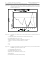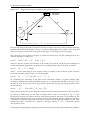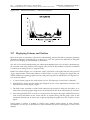
Download Nash, Nash. Scientific computing with PCs (1993)(205s)

Home
Scientific Computing
with PCs
John C. Nash
Faculty of Administration
University of Ottawa
Mary M. Nash
Nash Information Services Inc.
ISBN: 0 88769 008 4
Copyright © 1984, 1993 J C Nash and M M Nash
This book is available from several Internet servers by anonymous FTP. It is NOT free
to use, though the file SCPCDOC.PS contains the Preface, Contents and an example
chapter that you may freely print and use. If you decide to use the text of the book,
there is a $10 / copy licence payable to
Nash Information Services Inc.
1975 Bel-Air Drive, Ottawa, Ontario, K2C 0X1, Canada
Fax: (613) 225 6553
Email contacts: [email protected],
[email protected]
This file formatted on 29 November 1997
i
Next
ii
Copyright © 1984, 1994 J C & M M Nash
SCIENTIFIC COMPUTING WITH PCs
Nash Information Services Inc., 1975 Bel Air Drive, Ottawa, ON K2C 0X1 Canada
Copy for:Dr. Dobb’s Journal
Preface
This book tells "what to", "why to" and "when to" use personal computers (PCs) for carrying out scientific
computing tasks. There are many books that purport to tell users how to operate particular software
packages or to set up and maintain their personal computer hardware. These "how to" volumes have their
proper role and utility. Our goal is different: we aim to present ideas about the management decisions
involved in using PCs for scientific and technical computing.
The audience for this book is any scientist, engineer, statistician, economist, or similar worker who is
considering using a personal computer for all or part of his or her technical work. The ideas we present
can be used at the individual or group level. Being ideas about the management of resources, they are
kept simple to the extent that readers will think "I know that." We stress, however, that it is the day-to-day
practice of management ideas that counts; theoretical knowledge is like a smoke alarm without a battery.
There are three themes to this book:
•
Deciding what is or is not reasonable to attempt in the way of scientific computing with a PC;
•
Learning about and finding software to carry out our tasks with a minimum of fuss;
•
Choosing the tools to match the task to keep costs low.
By PC we will mean any computer system that is managed, used and maintained by a single person. The
typical examples are the relatives and descendants of the original IBM PC and the Apple Macintosh, but
other machines and workstations have similar properties. Workstation networks and mainframes with
system support staff have quite different management strategies. Portable computers used with such larger
systems are, however, very likely to be used in a way that requires the user to exercise management skills.
Our examples use mainly MS-DOS PCs since these are the most common.
The reader will notice some repetition of ideas we feel important; we also have tried to keep sections of
the book self-contained.
The distribution mechanism for this book is an experiment in a new form of publishing using the Internet.
We did not intend this to be the case. Unfortunately the publisher who commissioned the book as a
venture into a new subject area decided to retreat in the face of recessionary pressures after we had
submitted a typeset manuscript. Interest from other publishers did not transform itself into a contract. Our
response has been to pay to have the work professionally reviewed — as a good publisher should — and
to then edit and produce the work in a form that users can print out for their own use.
The current work has been formatted to reduce the number of pages from about 300 to about 200 by
choosing margins that use more of the page area on traditional letter-size paper. We believe that A4 paper
users will find that pages fit this size also.
Your comments are welcome.
John & Mary Nash, Ottawa, September 1994
0: PREFACE AND CONTENTS
iii
Contents
Part I: Panorama
4.8
Chapter 1:
4.9
4.10
4.11
4.12
4.13
1.1
1.2
1.3
History and goals
Non-goals
The scientific method and our
audience
Computer configurations of interest
Computing styles
1.4
1.5
Chapter 2:
2.1
Data processing capabilities of
PCs
Non-mathematical data processing
related to calculation
Communications — Access to remote
data
Automated data collection
Input, output, edit, and selection
Scientific text processing
Macro-editors and data converters
Graphics
Report writers
Programming and program
development
Administration of research
2.2
2.3
2.4
2.5
2.6
2.7
2.8
2.9
2.10
Chapter 3:
3.1
3.2
3.3
3.4
3.5
Introduction and Purpose — How
Scientific Problems are Solved
Computational capabilities of PCs
Good news
Application problems
Component computational problems
Component symbolic problems
Getting things to work
Part II: Computing environments
Chapter 4:
4.1
4.2
4.3
4.4
4.5
4.6
4.7
4.8
Will a PC suffice?
Hardware
Software
Interfacing, communications and data
sharing
Peripherals
Operational considerations
Issues to be addressed
Programming effectively
The software development
environment
Chapter 5:
5.1
5.2
5.3
5.4
5.5
5.6
5.7
Chapter 6:
6.1
6.2
6.3
6.4
6.5
6.6
Chapter 7:
7.1
7.2
7.3
7.4
7.5
7.6
7.7
7.8
Chapter 8:
8.1
8.2
8.3
8.4
8.5
8.6
Input/output problems — bugs and
glitches
Debugging and trouble-shooting
Precision problems
Size problems
Utilities and support
Summary
File management
File creation and naming
Types and distributions of files
Cataloguing and organizing files
Backup
Archiving
Version control
Loss versus security
Programming Aids and Practices
Programming tools and environments
Cross-reference listing and data
dictionary
Flowchart or other algorithmic
description
Structure and modularity
Sub-programs — data flow
Programmer practices
Size Difficulties
Determining memory and data
storage limits
Choice or adjustment of data
structures
Usage map
Restructuring
Reprogramming
Chaining
Change of method
Data storage mechanisms for special
matrices
Timing Considerations
Profile of a program
Substitution of key code
Special hardware
Disk access times
Time/accuracy and other trade-off
decisions
Timing tools
iv
Copyright © 1984, 1994 J C & M M Nash
SCIENTIFIC COMPUTING WITH PCs
Nash Information Services Inc., 1975 Bel Air Drive, Ottawa, ON K2C 0X1 Canada
Chapter 9:
9.1
9.2
9.3
9.4
9.5
9.6
9.7
9.8
Chapter 10:
10.1
10.2
10.3
10.4
10.5
10.6
10.7
Chapter 11:
11.1
11.2
11.3
11.4
11.5
11.6
11.7
11.8
Part III:
Chapter 12:
12.1
12.2
12.3
12.4
12.5
12.6
12.7
12.8
12.9
Debugging
Using output wisely
Built-in debugging tools
Listings and listing tools
Sub-tests
Full tests — robustness of code to bad
input
Full tests — sample and test data
Resilience to I/O failure and disk
problems
Tests of language translators
Utilities — a desirable set
Editors
File view, move, copy, archive and
backup
File display, conversion and print
File comparison
Directories and catalogs
Fixup programs
Sorting
Looking after the Baby Hardware and Operating Practice
Cleanliness and a decent physical
environment
Bad habits — smoke, sticky fingers,
children
Magnetic disks and their care
Tapes, CDs and other storage media
Power considerations
Interference and radio frequency
shielding
Servicing and spare parts
Configuration maintenance
The problem and its solution
method
Steps in Problem Solving
Problem formulation example
Algorithm choice
Algorithm implementation —
programming
Documentation
Testing — data entry
Testing — sub-programs
Testing — complete programs
Production runs
Modifications and improvements
Chapter 13:
13.1
13.2
13.3
13.4
13.5
13.6
13.7
Part IV:
Chapter 14:
14.1
14.2
14.3
14.4
14.5
14.6
Chapter 15:
15.1
15.2
15.3
15.4
15.5
15.6
Chapter 16:
16.1
16.2
16.3
16.4
16.5
16.6
Chapter 17:
17.1
17.2
17.3
17.4
17.5
17.6
Copy for:Dr. Dobb’s Journal
Problem formulation
Importance of correct formulation
Mathematical versus real-world
problems
Using a standard approach
Help from others
Sources of software
Verifying results
Using known techniques on unknown
problems
Examples
The Internal
Problem
Rate
of
Return
Problem statement
Formulations
Methods and Algorithms
Programs or Packages
Some solutions
Assessment
Data Fitting and Modelling
Problem Statement
Formulations
Methods and Algorithms
Programs or Packages
Some solutions
Assessment
Trajectories of Spacecraft
Problem statement
Formulations
Methods and Algorithms
Programs or Packages
Some solutions
Assessment
Simulating a Hiring Process
Problem Statement
Formulations
Methods and Algorithms
Programs or Packages
Some solutions
Assessment
0: PREFACE AND CONTENTS
Chapter 18:
18.1
18.2
18.3
18.4
18.5
18.6
18.7
A Program Efficiency Study: the
Cholesky Decomposition
Purpose of the study
The programs and systems compared
Measuring the differences
Program sizes and compiler options
Time differences from program
alternatives
Compiler and arithmetic influences
Processor and configuration time
differences
v
Chapter 20:
20.1
20.2
20.3
20.4
20.6
Your Own Strategy for Scientific
Computing on PCs
Identifying needs and wants
Acquiring the right computing
environments
Tools and methods
Add-ons, extras and flexibility
Personal Choice and Satisfaction
Bibliography
Figures and Tables
Chapter 19:
19.1
19.2
19.3
19.4
19.5
19.6
19.7
Case study: graphical tools for
data analysis
Index
Purpose of the study
Example data for analysis
Display characteristics
Choices of graphical tools
Displaying level and variability
Displaying relative measurements
Displaying patterns and outliers
This book is made available in PostScript™ form via Internet FTP servers. The copyright to this work
belongs to the authors. You may copy the PostScript files for this work and print off the file SCPCDOC.PS
freely. If you print off the files of the book itself you then owe the authors a licence fee of $10.
The book (and related materials) may be obtained by anonymous FTP from:
MacNash.admin.uottawa.ca
The full work is approximately 200 pages long and the PostScript files occupy about 4 megabytes of
storage.
vi
Copyright © 1984, 1994 J C & M M Nash
SCIENTIFIC COMPUTING WITH PCs
Nash Information Services Inc., 1975 Bel Air Drive, Ottawa, ON K2C 0X1 Canada
Copy for:Dr. Dobb’s Journal
Trademarks
The following table lists, as far as we could determine, the holders of various trademarks mentioned in
this work.
Trademark Holder
Adobe Systems Inc.
American Mathematical Society
Apple Computer Corporation
Aptech Systems Inc.
Borland International, Inc.
C Ware Corporation
Conceptual Software Inc.
Corel Corporation
Crescent Software Inc.
Data Description Inc.
Data Viz Inc
Gazelle Systems
Gibson Research Inc.
Hewlett-Packard
Intel Corporation
International Business Machines Inc.
Lotus Development Corp.
The MathWorks Inc.
Microsoft Corporation
Minitab Inc.
Motorola
Nash Information Services Inc.
NeXT Computer Inc.
Numerical Algorithms Group Inc.
Scientific Endeavors Corp.
Stata Corporation
Sun Microsystems, Inc.
Soft Warehouse Inc.
Strategy Plus Inc.
Stac Electronics Inc.
SYSTAT Inc. (now part of SPSS Inc.)
Travelling Software Inc.
True BASIC Inc.
UNIX System Laboratories Inc.
Waterloo Maple Software
Wolfram Research
WordPerfect Corporation
Zilog Corporation
Trademark(s) or Trade Name(s)
PostScript
TEX
Apple, Macintosh
GAUSS
BRIEF, dBase III, dBase IV, PARADOX, Turbo Basic, Turbo
Pascal, Turbo C, Borland C, Turbo C++, Borland C++, Quattro,
Quattro Pro
SEE, DeSmet C, DeSmet ASM88
DBMSCOPY
CorelDRAW, CorelPHOTO-PAINT
GraphPak
Data Desk
MacLink
OPTune
SpinRite
Hewlett-Packard
Intel, 386
IBM, RS6000, OS/2
Lotus, 1-2-3
MATLAB
Excel, Microsoft, Quick C, MS-DOS, Windows, Quick BASIC,
Visual BASIC
MINITAB
Motorola, 6800, 68000
SnoopGuard
NeXT
NAG
GraphiC
Stata
SUN
DERIVE, muMATH
EXECUSTAT
STACKER
SYSTAT, MYSTAT
Laplink
True BASIC
UNIX
Maple
Mathematica
WordPerfect
Z80
Previous
1: INTRODUCTION AND PURPOSE
Home
1
Part I: Panorama
To get a good idea of the lie of the land, one finds a convenient tree, hill or building and
exploits the larger field of view gained by height. As a preliminary to the detailed study
of the application of personal computers (PCs) to scientific computation, we will take
such a panoramic view. First, a chapter on the aims (and non-aims) of this book, which
concern the way in which scientific problems are solved and the role of computations
in such solutions.
Chapter 1
Introduction and Purpose:
How Scientific Problems are Solved
1.1
1.2
1.3
1.4
1.5
Background
Goals
The scientific method and our audience
Computer configurations of interest
Computing styles
This book aims to help researchers who are not computer specialists to use PCs profitably and efficiently.
It is especially concerned with the strategies and tactics that enable users to carry out their scientific work
in all aspects — technical, administrative and educational — with the aid of PCs. We do not claim that
PCs are the "best" answer for scientific computations but point out that they deserve consideration. Indeed
our message is that there is no uniquely "best" approach to scientific problem solving, but that there are
generally several options that will provide satisfactory results with modest expenditure of time and
money. It is toward reasoned consideration of the PC option that we direct our energies here.
1.1
Background
The PCs of this book are primarily those of the IBM PC family, with the Apple Macintosh also kept in
mind. We will use the abbreviation PC to refer to machines of both the IBM PC (that is, MS-DOS) family
and the Apple Macintosh. Because we have less familiarity with Atari and Commodore machines, there
are few references to them. Workstations based on the UNIX operating system, such as SUN, NeXT, IBM
RS6000, certain Hewlett-Packard machines and many others, have not been used as examples, mainly
because our use of such machines has been limited. The ideas presented in this book can nevertheless be
applied to such machines, particularly if the reader is the system manager. The software and manner of
use of workstations is, in our opinion, qualitatively different from that of PCs and Macintoshes in that the
workstations are less independent machines than parts of larger networks. While many PCs are also
connected in networks, the type of central support provided is more likely, we think, to be limited to
Next
2
Copyright © 1984, 1994 J C & M M Nash
Nash Information Services Inc., 1975 Bel Air Drive, Ottawa, ON K2C 0X1 Canada
SCIENTIFIC COMPUTING WITH PCs
Copy for:Dr. Dobb’s Journal
non-scientific applications. Thus there is a qualitative difference between the PC world and the (UNIX)
workstation world in the technical support provided to the user for scientific computations.
We note that both IBM PC and Macintosh can be operated under variants of Unix, and that OS/2 is
another choice of operating system for IBM PC users. As we write, Microsoft is introducing Windows NT.
We will mention such environments as appropriate, but they are not critical to our examples.
The realities of present-day PCs are as interesting as the publicity that surrounds them. However, there
is a lot less glamour to be found in the reality of PCs than in the advertising copy. This introduction
presents the authors’ goals in writing this book, suggests the type of reader who will find it most useful,
and declares several topics that will not be covered.
We will caution that advertised products need to be evaluated carefully. New products may be able to
serve us, but obstacles or restrictions mentioned in the fine print or omitted entirely may prevent easy
resolution of our problems. While users are now less likely to resort to doing their own programming than
a decade ago, there are still many computational problems that require such brute-force efforts.
Furthermore, the existence of commercial software that solves only one problem is not necessarily helpful;
it is difficult to justify spending hundreds of dollars to solve a problem that may be a small part of a
larger task.
An annoying aspect of today’s rapidly developing computer world, at least from the point of view of the
computist — the person who must perform calculations — is the constant stream of statements, articles,
lectures and papers that describe "new, improved" hardware or software. The realities of life in the world
of technical computation, be it in engineering, natural sciences, economics, statistics or business, are that
funds are not available to acquire each new piece of apparently useful electronics or program code.
Furthermore, the cost of learning and evaluating a single new product is high. The pressure to bring out
a new product ahead of competitors is such that errors are probably present in the first (or second or third
or . . . ) models delivered. This leads to contradictory evaluations of products in the literature, forcing
prospective users to spend much valuable time and effort to discover the true utility of the product for
their own situation.
There is, of course, pressure among the user’s own community to use the "latest and best." Salespeople,
industry writers and futurists have successfully created a collective faith in the ongoing rapid change in
computing. New products are supposedly obsolete as soon as they are delivered. While we all like to be
modern and up-to-date, much of the panic and hurrah is a myth. The truth is no less interesting, but does
not have the glamour and air-brush artwork that should, in any event, be left for the cover of fashion
magazines.
We have studied computation and performed calculations for more than twenty-five years. In that time,
many new and interesting devices have been brought to market. There have been substantial decreases
in the real costs of computing. In 1968, we paid $200 (Canadian) for a second-hand Monroe hand-cranked
mechanical calculator. In 1980, we bought the Sharp PC 1211/Radio Shack Pocket Computer for $279
(Canadian). This machine was capable of quite sophisticated programs in BASIC and had a large
repertoire of special functions. In 1992, a modest PC with 640K memory and floppy disk drives can be
bought for under $500 (Canadian) and a PC/AT with fixed disk for under $1000. Clearly, these are great
advances, and the Monroe is now a fondly regarded antique that nevertheless still functions perfectly. In
its time it fulfilled a need and was used to solve many problems similar to those still coming across our
desk today. In turn, the other machines will serve their time before being replaced. In fact we disposed
of our first generation personal computers late in 1991 after over 13 years of solid service.
The useful lifetime of computers continues to be several years. There are sound business and operational
reasons for this. One cannot consider equipment with a useful lifetime of less than five years as a good
investment, though we may expect the uses of equipment to change over that lifetime. Similarly,
manufacturers wish to convince us that their products are the last word in technology, but must have long
enough production runs to keep their costs to a minimum. Thus many "innovations" are cosmetic and
1: INTRODUCTION AND PURPOSE
3
designed to respond to marketing pressures.
In the practice of computation the changes observed in the last twenty-five years have been quite gradual.
Several commendable efforts have been made to produce quality mathematical software packages and
libraries. Despite the success of some of these efforts and the appearance of several new journals dedicated
to specialized computation, there is still a vast body of very low quality programs in use that have been
purchased, borrowed or stolen. These have frequently been installed without regard to the effects that a
different computing environment may introduce into a calculated result.
1.2
Goals
To the chagrin of developers of quality mathematical software, poorly designed programs will correctly
solve more than 99% of the problems presented to them. The expense and effort of good program
development is spent mostly to prevent disaster for a few cases in a million. This "insurance" aspect of
quality software is difficult to sell to users. A user who is happy with, but ignorant of, results from a poor
program is unlikely to change programs if it means, as it usually does, a considerable effort and cost.
Knowledgeable staff are seldom available to help the scientific user in the implementation of programs
to carry out calculations. Unlike programs to process data or control functions, the results of
computational programs are rarely right or wrong absolutely. That is, success in obtaining reasonable
results is not necessarily a sign that the calculation has been correctly performed. Worse, correct
performance in a number of cases may only lead to a false sense of confidence in a program destined to
give erroneous output in a future calculation. If this output is the basis of decisions — business
investment, government policy, vehicle design or aircraft navigation — we have the seeds of catastrophe.
With increasing reliance on computations and simulations in all fields of human endeavor, the possibility
and likelihood of occurrence of disasters large, and small, because of software failure, are an unfortunate
reality in all our lives. We address such topics in our related work on technological risks.
One objective, then, of this book is the realistic evaluation of what may be accomplished with the
computers that are commonly available to those of us who must perform calculations.
The second concern is the choice of strategies and tactics to make the most of the capabilities while
avoiding or overcoming the limitations, diversity or inconsistency. Much of this material is common to
all computing and data processing, be it on large, general-purpose machines, PCs or even a calculator,
pencil and paper. In this we wish to avoid gimmicks and tricks, instead emphasizing a scientific approach.
That is, we test claims, measure performance, deepen our understanding of what works and what does
not, gradually improving our computing tools and our abilities to use them as we develop a solution to
a problem.
A third goal will be avoiding unnecessary expense. Those with money and time to throw away we thank
for buying our book. They need read no further. Others with slimmer budgets will hopefully find some
useful tips to keep costs down.
In summary, this book is intended to be a guide and handbook to the calculation practitioner who must
produce correct answers to problems that can be stated mathematically. With this in mind, an index is
provided to enable quick reference use of the material. It is our hope that the text is interesting,
comprehensible, and informative to users.
Having stated the goals of this book, it may be assumed that objectives left unmentioned will not be
pursued. However, the diverse and turbulent activity concerning PCs has created a climate where readers
may expect a different book from that which we have written. Therefore, a short list of topics that are not
addressed is presented here.
•
There is no comparative shopping guide to computer hardware, peripherals or software. The examples
that do appear are there to serve as illustrations of the text. One reason for not attempting such a
catalog is that it is difficult to keep it accurate in detail as manufacturers make alterations and
4
Copyright © 1984, 1994 J C & M M Nash
SCIENTIFIC COMPUTING WITH PCs
Nash Information Services Inc., 1975 Bel Air Drive, Ottawa, ON K2C 0X1 Canada
Copy for:Dr. Dobb’s Journal
introduce their "new" products. Another reason is that we prefer to write from experience, which
clearly cannot be products just released today.
•
There is no attempt to present mathematical software formally in this volume. In other works (Nash
J C, 1990d; Nash J C and Walker-Smith, 1987; our magazine columns) we have discussed methods for
solution of many mathematical problems. We do, where appropriate, mention some sources and
examples of mathematical software. We point to sources and advice on their use, but do not include
machine readable software.
•
There is no attempt to provide an all-purpose handbook for every PC owner. While we sincerely feel
there are useful ideas here for all who work with computers, the focus is on calculation and its
practitioners as described below.
1.3
The Scientific Method and Our Audience
In all technical fields of endeavor, quantitative methods are assuming an increasing importance and use.
Heightening our understanding of phenomena, natural or man-made, quantitative measures bring a level
of detail compared to simple qualitative descriptions of observed objects or events. In business
decision-making, numerical rather than descriptive information is vital. In engineering, accurate
calculations of the strengths of structures and materials are important in saving millions of dollars in
unnecessary effort and fabric, while at the same time such results are critical to the integrity and safety
of the structures built.
Quantitative methods are an outgrowth of the scientific method, which may be summarized as follows:
•
Careful observation of the system of interest;
•
Formulation of a model explaining the system’s behavior;
•
Testing of the model by comparison of its behavior with that of the real system;
•
Further observation, model refinement and testing.
From the natural sciences, the scientific method has in recent years spread to social sciences and business.
Not all applications have been either well-founded or well-executed, especially when the scientific method
is taken to imply the use of a computer model. Models are popular because they are much less costly than
experiments or prototypes. Their limitations derive from our imperfect understanding or poor
approximation of the system in question. In a social model of consumer buying habits, we may be content
with very rough indicators of how a large group of people react to changes in prices or policies, since the
alternative is a complete lack of information. For aircraft flight simulation, however, we wish to mimic
the behavior of an airplane very precisely so that the pilot can practice maneuvers without risk to life or
property, while saving fuel and avoiding airport charges.
Models and related quantitative methods (the spectrum of statistical and data analysis tools) require
calculations to be performed. It is to those who must carry out these calculations that this book is directed.
The special interest is PCs, because calculations are increasingly being carried out in such computing
environments.
1.4
Computer Configurations of Interest
PCs may be purchased with an extremely wide range of options and it is necessary to define the type of
machine that is the focus of this book.
For our purposes, we will be interested in machines that are can carry out serious computations, which
implies they must be able to run reasonably sophisticated software. The key word here is "reasonably."
In 1980, such software was operated in a machine with a processor, memory, video display and keyboard,
1: INTRODUCTION AND PURPOSE
5
with 5.25 inch floppy disks for information storage. By the beginning of the 1990s, a fast fixed disk had
become more or less essential, in addition to the floppy disks (now 5.25 inches and 3.5 inches) that are
used as a medium for supply and exchange of data or programs. Furthermore, a large enough main
memory size is likely to be important so that scientific problems involving matrices and vectors can be
solved without heroic measures to manipulate memory and disk space.
To the basic machine, we would generally add a printer, which should support some form of graphical
output so that the user can plot as well as print information. This implies some form of dot-matrix printer,
or its higher-resolution cousins, the laser or ink-jet printer. We also believe communications with the
outside world are important. If telephone lines are the means of communication, then a modem is needed
(Section 2.2).
The above requirements can be met by many different examples of machines in the IBM PC and
Macintosh families.
1.5
Computing Styles
Throughout this book we will discuss ideas that relate to computing style. That is, we will be interested
in how users get the job done, with the "job" referring to scientific computations and related data
processing. Our experience has been that, even in the physical sciences, style counts as much as substance.
Scientists, engineers, economists and statisticians can easily get as excited or angry about cosmetic details
as about fundamental theories. In this we are as guilty as others. For example, we do not particularly like
mouse-controlled interfaces, though we have colleagues who swear they are the only reasonable approach.
We hope readers will find our treatment "permissive," allowing each user to select his/her own preferred
mode of operation.
Style also refers to the choices of what parts of one’s work are performed with a PC. Some users employ
just one computing platform, their PC. However, most scientists use more than one computer for their
work and we will try to point out the major advantages and pitfalls of multiple platform computing as
we proceed. In particular, we will try to raise alarms about situations where data might be awkward to
transfer between platforms. Such "glitches" invariably cause great consternation. After all, the data is "right
here on this diskette," yet neither action, prayer nor curses will release it.
At the same time, we will try to encourage users to maintain their data and program resources in a state
where they can be moved across machine boundaries and shared with others. The synergy that results
when like-minded researchers can easily exchange ideas and information is of immense value. In our own
experience it is highly rewarding, at times accompanied by moments of scintillating intellectual insight
that would never arise without the interaction of other workers.
Previous
6
Copyright © 1984, 1994 J C & M M Nash
Home
SCIENTIFIC COMPUTING WITH PCs
Nash Information Services Inc., 1975 Bel Air Drive, Ottawa, ON K2C 0X1 Canada
Copy for:Dr. Dobb’s Journal
Chapter 2
Data processing capabilities of PCs
2.1
2.2
2.3
2.4
2.5
2.6
2.7
2.8
2.9
2.10
Non-mathematical data processing related to calculation
Communications — Access to remote data
Automated data collection
Input, output, edit, and selection
Scientific text processing
Macro-editors and data converters
Graphics
Report writers
Programming and program development
Administration of research
This chapter concerns the data processing tasks that do not generally involve arithmetic. Even so, these
tasks may be a very important part of our overall scientific computing effort. We take the viewpoint that
a problem is not truly "solved" until the results have been convincingly reported. Thus preparing reports,
talks and papers, along with a variety of other work that supports and permits the solution of problems,
is scientific computing.
2.1
Non-mathematical Data Processing Related to Calculation
While this book is about scientific computing, it is rare that PCs are engaged in formal calculation work
for more than a small percentage of the time. The primary reason for this is that PCs serve their users as
data and word-processing tools, as well as engines to perform computations. In contrast, a highperformance supercomputer will generally be fed tasks by other computers. We do not expect such
number-crunching boxes to occupy their expensive cycles waiting for keyboard entry or mouse clicks.
Because PCs act as a doorway to calculations, we shall point out how they prepare for and control
calculations and how they help manage and report results. PCs are also used to direct tasks on other
computers, or gather data or bibliographic citations from remote sources. These tasks, while tangential to
scientific computing, are nevertheless essential to the advancement of research. Especially in the social
sciences and statistics, we may need a great deal of clerical effort before calculation starts.
Clearly such work is not mathematical in nature. The main goal is to move, transform and put in order
various quantities of data so that calculations can be performed, results organized and analyzed, and
reports written. In the remainder of this chapter we shall look at the capabilities of PCs to help in this
work.
2.2
Communications — Access to Remote Data
Because workers must communicate with their colleagues, a large part of any researcher’s time is spent
in written and oral communications. Letters are giving way to facsimile transmissions (fax) and electronic
mail (email) exchanges. Some workers are also using direct machine-to-machine linkages, either via
informal or organized attempts at group working (see for instance, the entire issue of the Communications
Next
2: DATA PROCESSING CAPABILITIES OF PCs
7
of the ACM for December 1991).
In sharing ideas, we must choose between direct interaction — the real-time, online, face-to-face or
telephone exchange — and indirect communication — letters, email, fax, bulletin board exchanges, voice
mail, or similar offline (time-independent) information exchange. Our own preference is offline: we like
to read and sort messages at our convenience. Call Waiting or mobile telephone service offer to keep us
always in touch. Following our policy throughout this book, we stress that each user of technology should
carefully analyze his or her own situation. PCs are a part of such communication choices.
From our perspective, the important feature is connectivity — the fact that a PC can be linked to whatever
source of data or information the user requires. There are some difficulties:
•
Physical obstacles exist in the form of incompatible hardware such as interface ports and connectors
at either end of the connection we wish to make, lack of suitable linkages such as transmission wires,
or modems operating under different physical protocols (Derfler and Byrd, 1991).
•
Logical obstacles occur when we do not have suitable accounts on the email networks of interest, or
there is no gateway between our network and that of the person with whom we wish to exchange
information, or the information is stored or transmitted in incompatible formats.
•
Lack of training or understanding of the software and protocols may prevent us from establishing the
connection. For example, we may not know how to log into a bulletin board, or if we do know, we
may not know the correct modem settings for the speed, parity and word size.
Increasingly, users of PCs are connected to Local Area Networks (LANs). These should serve to simplify
and speed up the connections we are likely to make. However, they may inhibit the worker who needs
to do something out of the ordinary. LANs are usually managed for the benefit of a perceived "majority"
of users. As LANs get larger, or are linked together, Wide Area Networks (WANs) are beginning to
appear.
Increasingly, academic and other research environments are being linked together by special high-speed
networks. These allow for rapid electronic mail, file transfer, and remote computer operation. There have
been some unfortunate abuses of these systems in the form of unauthorized access and destructive
programs (viruses, worms, etc.), but the benefits appear to outweigh the costs by a wide margin. The
networks now link most parts of the world and connections and email are increasingly reliable. This has
fostered the development of electronic newsletters and journals, special database servers to supply
particular software or data, and a variety of electronic "conferences" (Krol, 1992; Stoll, 1990).
For PC users, it is important to note that while the networks transmit binary data, there may be nodes
between us and a source of information that insist on working with text information. To allow the binary
data to cross such a node, it is common to encode the binary data as printable text characters. The
receiving computer reverses the coding. Two common formats for such exchange are UUENCODE and
BINHEX, for which programs may be found in a variety of public repositories. There are also ways to
transmit binary data across modems directly (Nash J C, 1993a).
2.3
Automated Data Collection
Researchers are in the business of gathering data. Measurements used to be taken with simple instruments
and recorded on paper, traditionally in bound, hard-cover laboratory notebooks. Analysis was with pencil
and paper. With electronic technology has come a capacity for instruments to provide output directly in
digital form, suitable for direct input to computers. There is an increasing use of computer technology for
control and calibration of these same instruments. PCs have frequently been used as both control and
data-gathering devices (e.g., Okamura and Aghai-Tabriz, 1985). Instruments with auto-answer modems
connected to the telephone network allow remote measuring stations to transfer data to a central site. We
suggest readers investigate the possibilities of automated instruments with care, since data collection is
generally done in real-time and must necessarily interfere with conventional machine operations.
8
Copyright © 1984, 1994 J C & M M Nash
Nash Information Services Inc., 1975 Bel Air Drive, Ottawa, ON K2C 0X1 Canada
SCIENTIFIC COMPUTING WITH PCs
Copy for:Dr. Dobb’s Journal
Optical scanning equipment, though designed for optical character recognition and for the input of graphic
material, can provide data to be processed in a variety of ways. There are cameras for input of still or
video images. Researchers studying sound or electro-magnetic signals have a variety of instruments for
inputting raw data. MIDI interfaces allow two-way transmission of musical information between
instruments, synthesizers and computers. We have used scanners with moderate success to process photos
and other images for use in reports and also to convert a typescript of a century-old diary into machinereadable form.
A variety of other interface mechanisms are used between computers and measurement devices.
2.4
Input, Output, Edit, and Selection
PCs are well suited to the task of entering, correcting and transforming data. It is relatively easy to write
particular programs that provide a very friendly user interface yet carry out extensive error checking for
well-structured problems. That is, if the problems are always of a specific type, a data entry program can
be prepared straightforwardly to allow non-specialists to enter the data.
Preparation of a general data entry program is much more difficult. A priori we do not know the structure,
type or precision of the data to be expected. Is it numeric or alphabetic? Whole numbers, fractions or
mixed? Four digits or ten? How is each data element to be identified? Typically we, along with many
users, employ a text editor and enter our data as simple lines of text information, though this allows no
immediate control on the elements we are keying in. Statisticians use the word "edit" for the process of
checking data elements to see if they are "reasonable"; the word "imputation" is used for the substitution
of reasonable values for missing entries.
Similarly, a general data transformation program is difficult to produce, but special ones are easily
implemented on PCs. Spreadsheet packages come close to being general data transformation programs.
They have the great advantage that they are generally well known by non-programmers. They are easy
to use for data entry. Editing individual entries to correct small errors is not difficult, but more global
editing, such as a repeated find and replace, may be more awkward. They also generally lack a way to
prepare general "scripts" that can be applied to many worksheets (Nash J C, 1993b). Simple graphs can
be prepared easily. Most spreadsheet programs also incorporate some database management functions,
but their strengths are the straightforward manipulation of tabular data.
Most PC database management programs also offer some attractive features for data entry, edit and
selection. In particular, we may quite easily "program in" checks for absurd data. For example, a
traditional concern with census data in the United States is the number of women who report multiple
children and also report their age as under 14 (Sande I, 1982). Database management programs generally
require more effort to use, in our opinion, than spreadsheet programs, but they offer greater flexibility.
2.5
Scientific Text Processing
Since the preparation of technical papers and reports is a primary data-processing task of PCs, it is
important to consider the possible approaches we may take. There are several special-purpose textprocessors designed to handle scientific material. In particular, the input and editing of mathematical and,
to a lesser extent, chemical formulas are useful requirements. Such formulas are only slightly more
difficult to write down on paper than the prose that usually surrounds them. However, as far as we are
aware, all computer text processing systems make formula entry much more difficult than text entry. This
is because text is mostly linear in the way in which it is presented, that is, one word follows another, left
to right across the page in European languages. Formulas require us to recognize a variety of horizontal
and vertical spacing rules, all of which can have very important meanings for the writer and reader.
2: DATA PROCESSING CAPABILITIES OF PCs
9
It is our opinion that the learning cost is the greatest barrier to the use of special-purpose scientific text
processors. There are a bewildering number of features and choices to make, as well as several interface
mechanisms to consider. Of these, we note in particular TEX (Knuth, 1986), which is perhaps the most
important of the mark-up languages. In a mark-up language, all the material is entered as text in a
standard alphabet with special commands embedded to indicate fonts, positioning, type styles, special
symbols, underlining, etc. The commands use characters from the standard alphabet. TEX prepares
material for type-setting, but the source material is not particularly readable to the uninitiated. The
alternative is a WYSIWYG (What You See Is What You Get) approach where the user selects and positions
symbols, possibly with the aid of some built-in formatting rules. An extensive surveys of scientific text
processing has been carried out under the direction of Dr. Richard Goldstein (Goldstein et al., 1987a,
1987b, 1987c).
As special-purpose scientific text processors have evolved, the general word-processing vendors have also
sought to add scientific features to their products. This book has been prepared using WordPerfect 5.1
(abbreviated WP5.1 from now on) using an MS-DOS computer with a VGA screen. We chose to use WP5.1
mainly for reasons of safety rather than features or convenience. In particular, with the very large installed
base of users, there was likely to be advice and assistance available to overcome difficulties and userUNfriendly quirks, of which we encountered many.
2.6
Macro-editors and Data Converters
Scientific computation inevitably requires data to be edited or its format transformed so that programs
can make use of it. Lack of appropriate tools for these tasks is perhaps the most common source of
frustration for researchers attempting to use PCs in their work. Sometimes editing and reformatting can
be accomplished with a suitable macro-editor as discussed below.
Most PC users have some form of text editor. Frequently it is the same editor that is used for preparing
letters or reports. Unfortunately, there are some significant dangers for the unwary. Students who have
learned a word-processor such as WP5.1 frequently do not realize that the "document" files saved by
word-processors include a large amount of information on how the document is to appear on the page.
This information is stored as bytes in the file additional to the text in which we are interested. When an
application program such as a programming language compiler reads the file, anticipating only the text,
errors occur.
Even as a tool for looking at results, word processors have deficiencies. For example, it is quite simple to
build a spreadsheet of fifteen columns of numbers. Allowing 10 spaces per column, this is 150 spaces
wide. If we import the "printout" from such a spreadsheet into a word processor, we may find that the
pleasant tabular structure of columns and rows has become an almost unreadable jumble of numbers and
column headings. The difficulties are:
•
Word processors often allow users to set and change margins and font sizes. Text is then wrapped to
fit the margins. That is, the line lengths are adjusted to fit the margins, not vice-versa. We need to set
our margins wide enough to accommodate the 150 character-wide lines of our spreadsheet if we wish
to be able to see the structure.
•
Word processors usually allow proportionally-spaced fonts. In these, the number 1 may take less space
than a number 9 or a 7. The column alignment is once again lost unless we specify that a monospaced
font is to be used.
This does not imply that one cannot use a familiar word-processing editor, but care needs to be taken.
It is quite easy to find public domain or freeware editors that allow for the manipulation of the text alone.
(NED — the Nash EDitor — is our own freeware contribution. At under 6K bytes, it is very small and
fast, yet includes a help screen and mouse support. See Nash, 1990a.) Users may also find that there are
convenient editing tools included with programming languages or even with the operating system.
Microsoft, after many years of imposing the truly medieval EDLIN on MS-DOS users, incorporated the
10
Copyright © 1984, 1994 J C & M M Nash
Nash Information Services Inc., 1975 Bel Air Drive, Ottawa, ON K2C 0X1 Canada
SCIENTIFIC COMPUTING WITH PCs
Copy for:Dr. Dobb’s Journal
Quick BASIC editor EDIT, in MS-DOS 5.0. Such tools serve very well to correct or adjust a few characters
in a file but are less useful when many changes have to be made.
For manipulations that have to be repeated, we recommend a macro-editor, in which the user can set up
several sequences of commands that can be executed via a single keystroke. This vastly simplifies
operations of removing unwanted commas in data files, stripping out or adding in spaces, and similar
tedious but necessary operations.
When we have a large (>50K) file to manipulate we use the commercial version of NED. It can edit any
file for which we have enough disk space. One common use of such editors is to search through large text
files for information.
We find that we use variations on the above theme nearly every day. Clearly we could use a special text
search utility like the UNIX facility GREP. We occasionally use file viewers that allow searching, but
prefer a small set of very familiar working tools. Moreover, the editor allows us to buffer and extract
pieces of the text in which we are interested.
Clearly a text editor cannot easily adjust a file that is encoded in some way. For example, spreadsheet data
files contain a variety of different forms of data: numbers, strings, data ranges, printing and output control
information, and graphs. The typical worksheet is saved in binary form and is not amenable to viewing
without special programs. Similar comments may apply to the files saved by database management
programs, though some packages advertise the important fact that information is stored in text files.
We usually find it easiest to extract information from spreadsheets or database programs by "printing"
information to a text file and editing it with our text editor. We use the spreadsheet or database program
to select which data we save to the file, as well as the order in which it is presented, while the text editor
is used to adjust the detailed layout or format. Here we are following a strategy of choosing to use
familiar tools and a tactic of using each to perform tasks for which it is best suited.
Alternate approaches exist. In circumstances dependent on the application and frequency of use, we may
prefer to use the data translation facilities of programs we use. Spreadsheet, database, word-processing,
and statistical programs frequently provide selected translation facilities, especially into, but less
commonly out of, their native formats. We note, for example, the Translate facility of Lotus 1-2-3. When
buying software, it is important to note which data formats can be used.
More generally, there exist programs that attempt to convert a range of different data formats, even across
operating systems or computing platforms. Usage will depend on application. For example, MACLINK
converts file and disk formats for a variety of word processing programs between the Apple Macintosh
and MS-DOS families of computers. DBMSCOPY allows data exchange between a large collection of
different database management and statistical programs. Graphics Workshop allows a variety of picture
files to be transformed one into the other, mostly successfully, but always with the danger of some loss
of definition or "out of memory" error. CorelDRAW and CorelPHOTO-PAINT have proved more flexible.
Unfortunately, data file formats are constantly evolving, so that the provision of "long-lasting relief" to
the data format transformation problem is not likely to be found. Our strategy has been to try to save data
as much as possible in text form, since users then have a reasonable chance to find some way to work
with files we provide. In this regard, we note that both TEX and PostScript, which essentially describe
graphical information, are coded as text. PostScript files are rather difficult for humans to interpret, but
there are many different machines — usually laser printers — that can do so. TEX, however, we find easy
to convert to simple text or to camera-ready material, even though we do not have the software to
perform the manipulations. The main codes are simple enough to follow so that we can provide the
equivalent word-processing commands.
2: DATA PROCESSING CAPABILITIES OF PCs
2.7
11
Graphics
Some computer peripheral devices literally "draw" lines on either paper or a screen by moving a pen or
an electron beam from one point to another, then another, and so on. For this reason, they are referred
to as vector graphic devices. The TV screen and most computer monitors draw dots on a screen in a row
of lines. To draw a picture, one must put the appropriate colored dots in the correct position in a large
matrix of dots. They are called raster graphic devices. Working on the same principle, drawings can be
output to dot-matrix printers, of which the laser printers are a high-resolution, small-dot version.
It is not trivial to use raster devices directly, since we think of drawing, e.g., with a pencil, in vector form.
The "programming" of drawing is easiest with vector graphic tools, for example, the Hewlett-Packard
Graphics Language (HPGL) that can drive not only plotters but also Laser printers and even numerically
controlled machine tools. PostScript may also be considered a vector graphics language.
For research users, there are likely to be many reasons why graphical computing tools will be important:
•
Research data is frequently best presented as a simple graph, for example, growth of plants or animals
over time, chemical reaction kinetics, or spacecraft trajectories. Statistical distributions and data
relationships can be visualized by a variety of data plots.
•
Drawings of instruments, either in preparation for their construction, to illustrate what we propose
to do, or to report what has been done, are now more easily prepared with Computer Aided Design
(CAD) software than by recourse to a draftsman.
•
In a technical report, we commonly need to include a photo. While "production quality" will require
the actual photo, a reasonable image can be included in the draft or on the layout sheet by importing
it into a word-processing document from an optical scanner.
•
Image painting or drawing programs allow us to include logos or other designs to improve reports
and slide-show presentations. Image painting programs give us control over the individual pixels in
a bit-mapped image. For this book, we used CorelDRAW. It is also possible to consider hypertext
forms (Taylor, 1991).
•
Page layout programs may be considered as graphical tools if we have pictorial elements or fancy
layouts in our reports.
•
To convert paper documents to machine readable form, optical scanning with character recognition
software can be used to provide a more or less correct machine-readable version. This is then
manually edited to fix any errors in the recognition process.
Unfortunately, users of graphics must still ensure that all pieces of software and hardware can be
organized to work together. Using color information in reports is still expensive, so color is usually
re-coded as different shading or hatching, sometimes in ways that are not recognizable. As color output
devices gain acceptance, this difficulty may become less important.
One area where graphics have become extremely important is in the interface to computer operating
systems. Many scientific computists prefer the Macintosh desktop or the Microsoft Windows operating
environment to a command driven system. For some applications, a pointer-driven graphical interface is
essential; for others it may slow our work. In many cases the choice is a matter of personal preference,
with software available to use in both types of environment.
2.8
Report Writers
Many scientific computations, for example linear programming computations, produce a very large
quantity of output. While it is sometimes important to save the detailed information for future analysis,
the usual output may not be in a form suitable for review by management or colleagues. To overcome
the difficulty the volume of data presents, we may use a report writer to summarize the results and
12
Copyright © 1984, 1994 J C & M M Nash
SCIENTIFIC COMPUTING WITH PCs
Nash Information Services Inc., 1975 Bel Air Drive, Ottawa, ON K2C 0X1 Canada
Copy for:Dr. Dobb’s Journal
highlight any important features.
Such report writers were a growth industry in the early 1970s, but since then have apparently become less
popular. In part, this may be attributed to better reporting of numerical results by the scientific programs
themselves. There is also a greater emphasis on graphical reporting of results that renders them more
immediately accessible to users and their colleagues.
Nevertheless, users of PCs may wish to consider the creation and use of simple programs to sift and
summarize results. For example, to compare run-time performance of several programs, we could use a
simple filter program to extract the execution time information from files of console (screen) output. The
program could be organized to tabulate our results roughly. The alternative would be to use a text editor
to remove the unwanted detail of the results. In practice, we have often chosen the middle ground of
using a macro-editor, which allows us to find and extract the required information by invoking sequences
of commands with single keystrokes.
2.9
Programming and Program Development
Most scientific computations involve, at some stage, the use of custom-developed programs. Macro-editors
are a help here in writing the source code. The compilation and linkage editing of the code to make a
working program is clearly data-processing. PCs can take advantage of a very wide range of programming
language processors. In our own case we find that we have access to the following programming tools
(compilers, interpreters, assemblers) for MS-DOS computers:
•
BASIC (several GWBASIC and QBASIC interpreters; IBM, Microsoft, Turbo, Quick and True BASIC
compilers);
•
FORTRAN ( Microsoft 3.2 and 4.1, Lahey F77L 2.2 and 3.1, Watcom F77 Version 9.0);
•
C (DeSmet 2.4 and 2.5; Eco C; Turbo C++ 1.0, 2.0 and Windows; Microsoft Quick C version 2.5);
•
PASCAL (Turbo Pascal 3.01a, 5.0, 5.5, and Windows; Pascal-SC);
•
80x86 Assembly code (Microsoft Macro Assembler, De Smet ASM88).
With the above there are several different linkage editors. Some of the listed programming tools are out
of date. Others, though dated at the time of writing, are still useful tools.
By far the most popular high level language in the early 1980s was BASIC, which is really a family of
similar but hardly compatible dialects. Efforts have been under way for over a decade to standardize
BASIC (Kurtz, 1982), but apart from Minimal BASIC (ISO 6373/1984) this effort has not had a great
impact. A reason for the popularity of BASIC was that a version is supplied with most MS-DOS PCs.
BASIC is, however, rare on Macintosh computers.
The use of BASIC is diminishing as users treat the computer as an appliance for information handling
tasks; they are not programmers. Moreover, BASIC lends itself well to quick-and-dirty tasks, (Nash J C
and Nash M M, 1984), but is not well-suited to large scale projects. For example, most BASIC interpreters
allow only a single 64K memory segment to be used for program or data on MS-DOS machines. By
contrast, Microsoft Visual BASIC offers a tool for Windows programming.
Scientific computing has traditionally been carried out in FORTRAN. FORTRAN compilers available for
PCs are generally based on the 1977 standard (ISO ANSI X3.9 - 1978, American National Standard
Programming Language FORTRAN). For computational efficiency, FORTRAN appears to be a good
choice. The compilers generally support memory access to large arrays and there is a wide selection of
source code available in the public domain. Unfortunately, FORTRAN compilers are not as convenient
for novice users as, for example, the Pascal development environments from Borland Inc. Nor do they
always supply the same level of functionality for controlling user interfaces such as Pascal or C compilers,
2: DATA PROCESSING CAPABILITIES OF PCs
13
screens, keyboards, file handling or pointer device functions.
The use of various compilers and interpreters can be very tedious. The Microsoft FORTRAN compiler
version 4.10 offers a choice of four different memory models and five different approaches to floatingpoint arithmetic. This presents the user with the tedious chore of specifying the correct disk\directory
path for each compiler and linkage library (the pre-compiled code that provides the appropriate memory
and floating-point choices).
When we have to compile and/or consolidate several pieces of code, it is better to automate the process.
We may decide to use a BATch command file (Microsoft, 1991), which is essentially a pre-recorded version
of our keystrokes. To consolidate source code segments, we have had considerable success using simple,
though quite long, BATch command files (see Nash J C and Walker-Smith, 1987). MAKE, developed to
ease the burden of building C codes in UNIX systems, appears in several forms accompanying C,
FORTRAN and Pascal systems on PCs. This program takes a simple script (called the MAKEFILE) and
builds our program from the appropriate pieces. A particularly pleasant feature of MAKE is that it is able
to use the time-stamps of files to avoid recompiling source codes that have not changed since the last
compilation. Thus it saves time and effort if it can. We have used MAKE in a C-language programming
project aimed at the study of tumor growth.
The BATch command files can also be replaced with programs. Examples are given in Nash J C and
Walker-Smith (1989b) in the BASIC program NLPDEX. In Nash J C (1990b), we suggest consolidation and
execution of program code using a hypertext environment that allows the user to learn about available
programs and data and then actually use them; this was demonstrated in Nash J C (1993b).
2.10 Administration of Research
We have already noted that researchers use PCs for preparing reports and performing a myriad of
mundane tasks. Among these are the administration of their scholarly work. This involves, in our mind,
planning tasks, preparing grant applications, tracking activity, preparing progress reports and
administering research funds.
With research increasingly involving collaborations over distance, these tasks may require extensive use
of email and file transfers. We may anticipate the eventual use of groupware — software allowing realtime exchange of computer messages for collaborative work via a network.
Clearly the PC is well suited to the development of work plans, using simple lists generated with a text
or outline editor. Grant applications, while generally restricted in format, can usually be prepared using
a word-processor. If there are several aspects to the same overall project, there will be considerable
duplication of information.
To track activity, we like to use a diary system and extract information from it as needed. One of us (MN)
prefers the traditional book form "planner" into which activities are recorded first as plans, later as
activities. The other (JN) prefers to keep a "to do" list using a text editor and to transfer the "to dos" to
activities with additional comments once completed. The choice is, once again, personal, and the computer
a possibility rather than a requirement.
Previous
14
Copyright © 1984, 1994 J C & M M Nash
Home
SCIENTIFIC COMPUTING WITH PCs
Nash Information Services Inc., 1975 Bel Air Drive, Ottawa, ON K2C 0X1 Canada
Copy for:Dr. Dobb’s Journal
Chapter 3
Computational capabilities of PCs
3.1
3.2
3.3
3.4
3.5
Good news
Application problems
Component computational problems
Component symbolic problems
Getting things to work
The PCs introduced in the previous chapters have not conventionally been regarded as tools suited for
serious computation. Early PCs had limited memory and slow execution rates that are not, by choice, the
characteristics of a number-crunching engine, especially as the processors usually lacked floating-point
(REAL number) arithmetic instructions. Moreover, the programming tools were usually interpreters of
limited capability with quirks or errors in exception handling and special functions. This chapter points
out where PCs and their software are likely to be able to carry out scientific computations.
3.1
Good News
A number of technological and commercial developments have vastly improved the capabilities of PCs
for scientific computation:
•
The development of high-performance floating-point co-processors with well-defined properties thanks
to the efforts of a number of workers, particularly W. Kahan of Berkeley, toward the IEEE FloatingPoint arithmetic standards and concurrent development of the Intel 80x87 and related devices;
•
Larger memory capacities and address spaces;
•
Faster, more efficient interfaces such as video-display adapters, memory managers and disk
controllers;
•
Fast, large and inexpensive fixed disks;
•
More capable operating software allowing better use of available hardware, such as disk or memory
caches (Section 8.3), printer buffers (Section 11.8), and utility software (Chapter 10);
•
Full-feature programming language compilers;
•
Reliable application packages, such as modern statistical software.
Interest in manipulating graphical images for video games has provided an impetus for large memories
and fast processing. Computers with these features are commodities like any other consumer electronic
product. In consequence, it is now possible to buy a PC with roughly the raw processing power of a
typical university central computer of a decade ago and to pay less than $5000 for it.
Recognizing this computing power, developers have produced some powerful scientific software. For the
user — and the reader of this book — the issue is finding and choosing the right software at the right
price for particular problems. Since many scientific problems have different names or descriptions in
different subject areas, this can be more difficult than we would like. In this chapter, and indeed in the
rest of the book, we will try to explain some of the jargon that is associated with various problems. Also
we will try to point to the component sub-problems that commonly arise in many classes of scientific
computing, since users can "put the pieces together" if they know what pieces they need.
Next
3: COMPUTATIONAL CAPABILITIES OF PCs
15
Our goal is to recognize when our machine can perform desired tasks, and if it can, whether it can do it
sufficiently quickly for our needs, with acceptably low human effort involved. We take the position that
the central obstacle to successful scientific problem solving usually lies in one or more mathematical subtasks. There are, of course, many ancillary tasks to be performed, often requiring most of our
programming and management effort. These are not ignored, but they are generally not the critical
obstacle to the use of a given computer in carrying out scientific work. That is, one or more of the
mathematical sub-problems may prove insurmountable and prevent the use of the PC in the overall
solution of the scientific problem.
3.2
Application problems
Scientific and technical computing clearly has more variations than we can discuss in a book of this size.
However, the main types of problems can be listed. These are:
•
Analytic problems, that is, those involving solution of equations or finding of roots or extrema — the
manipulation of existing data to extract information;
•
Simulation problems, where we synthesize plausible data a number of times to explore possible
outcomes to particular situations;
•
Transformation or presentation problems, where we are trying to recast existing data into a new form.
It is useful to recognize these three types because analytic problems are "finished" when we have a
solution. However, we decide how many sets of conditions to specify for simulations. That is, they can
be open-ended. Transformations and presentation problems may involve several cycles of experimentation
to achieve a desired "view" of our data.
In the next two sections we mention the names of some mathematical problems to which application
problems are often reduced. Much of the work of problem solving is learning how to do this efficiently
in both human and computer effort. Of course, we have afterwards to interpret the results so that they
may be understood.
3.3
Component computational problems
This long section lists and briefly describes some classic problems of computational mathematics. It also
provides a notation we can use in later chapters.
Numerical Linear Algebra — Matrix Calculations
A matrix is a rectangular array of numbers. Within a matrix A that has dimensions m by n, that is, having
m rows and n columns, the i,j element of A occupies the row i, column j position. This simple structure
of numbers forms a building block of linear algebra. It has been applied in almost all subject fields, both
directly or as a part of other numerical methods. The most common general problem types addressed by
numerical linear algebra are:
•
Linear equations, that is, finding the solution values
xj , for j = 1, 2, . . ., n to the n equations
(3.3.1)
We shall generally use the matrix form of these equations
(3.3.2)
Ax = b
16
Copyright © 1984, 1994 J C & M M Nash
Nash Information Services Inc., 1975 Bel Air Drive, Ottawa, ON K2C 0X1 Canada
•
Least squares approximations. Here we wish to find a set of values
sum of squares
SCIENTIFIC COMPUTING WITH PCs
Copy for:Dr. Dobb’s Journal
xj , j = 1, 2, . . ., n such that the
(3.3.3)
is minimized, where
(3.3.4)
Again, this may be written in matrix form as
(3.3.5)
where
T
denotes matrix transposition, and
r = b - Ax
(3.3.6)
Note that
•
A is now rectangular (m by n), whereas, for linear equations it was a square matrix.
Matrix decompositions, including the eigenvalue decomposition. These problems aim to find products
of other matrices that are equal to the given matrix A. The matrices that make up the decomposition
have special properties. Some particular decompositions are:
· the singular value decomposition
A = U S VT
(3.3.7)
where U is an m by n matrix of orthogonal columns such that UT U = 1n , the identity of order n, V
T
T
is an n by n orthogonal matrix so that V V = V V = 1n, the identity of order n, and S is a diagonal
matrix having non-negative elements.
· the eigenvalue problem (square matrices)
AX=XE
(3.3.8)
where
X has some normalization and E is diagonal. For symmetric matrices where
AT = A
(3.3.9)
the eigenvalue problem is straightforward, but it becomes increasingly difficult when the matrix is
non-symmetric or complex.
· the QR decomposition (or orthogonalization)
(3.3.10)
where
R is upper-triangular or right-triangular, that is
(3.3.11)
and
A=QR
Rij = 0
if
i>j
Q is m by n orthogonal
3: COMPUTATIONAL CAPABILITIES OF PCs
17
Q T Q = 1n
(3.3.12)
· the LU decomposition (A square)
A=LU
(3.3.13)
where
L is lower-triangular and U is upper-triangular
(3.3.14)
Lij = 0
if
j>i
(3.3.15)
Uij = 0
if
i>j
(Thus
U and R have the same structure; the different mnemonics are purely historical.)
There are many variations on the above problem types depending on the matrix properties. For instance,
a matrix may be categorized by:
m, and the number of columns, n;
•
Size, that is, how large are the number of rows,
•
Presence of complex elements, otherwise the matrix is real;
•
"Shape", that is, "tall" if
•
The pattern of non-zero elements, for example, upper- or lower-triangular as presented above,
diagonal if Aij = 0 if i≠j , banded if Aij = 0 if j-i > k, where k is a small integer.
•
The existence of mathematical properties such as positive definiteness or norm of the matrix, or
properties about the values, e.g., a Toeplitz matrix, which has all elements on any diagonal of equal
value.
•
The proportion of non-zero elements to the total, where a small proportion of non-zero elements gives
a sparse matrix, whereas a high proportion gives a dense one.
Band matrix
x
x
x
0
0
0
0
0
0
0
x
x
x
x
0
0
0
0
0
0
x
x
x
x
x
0
0
0
0
0
0
x
x
x
x
x
0
0
0
0
0
0
x
x
x
x
x
0
0
0
0
0
0
x
x
x
x
x
0
0
0
0
0
0
x
x
x
x
x
0
0
0
0
0
0
x
x
x
x
x
Lower triangular matrix
0
0
0
0
0
0
x
x
x
x
0
0
0
0
0
0
0
x
x
x
Tridiagonal matrix
x
x
0
0
0
0
0
0
0
0
x
x
x
0
0
0
0
0
0
0
0
x
x
x
0
0
0
0
0
0
0
0
x
x
x
0
0
0
0
0
0
0
0
x
x
x
0
0
0
0
0
0
0
0
x
x
x
0
0
0
0
0
0
0
0
x
x
x
0
0
0
0
0
0
0
0
x
x
x
0
m >> n, "fat" if m << n, square if m = n;
0
0
0
0
0
0
0
x
x
x
x
x
x
x
x
x
x
x
x
x
0
x
x
x
x
x
x
x
x
x
0
0
x
x
x
x
x
x
x
x
0
0
0
x
x
x
x
x
x
x
0
0
0
0
x
x
x
x
x
x
0
0
0
0
0
x
x
x
x
x
0
0
0
0
0
0
x
x
x
x
0
0
0
0
0
0
0
x
x
x
0
0
0
0
0
0
0
0
x
x
0
0
0
0
0
0
0
0
0
x
Hessenberg matrix
x
x
0
0
0
0
0
0
0
0
Upper triangular matrix
0
0
0
0
0
0
0
0
x
x
x
0
0
0
0
0
0
0
0
0
x
x
0
0
0
0
0
0
0
0
x
x
x
0
0
0
0
0
0
0
x
x
x
x
0
0
0
0
0
0
x
x
x
x
x
0
0
0
0
0
x
x
x
x
x
x
0
0
0
0
x
x
x
x
x
x
x
0
0
0
x
x
x
x
x
x
x
x
0
0
x
x
x
x
x
x
x
x
x
0
x
x
x
x
x
x
x
x
x
x
x
x
x
0
0
0
0
0
0
0
x
x
x
x
0
0
0
0
0
0
x
x
x
x
x
0
0
0
0
0
x
x
x
x
x
x
0
0
0
0
x
x
x
x
x
x
x
0
0
0
x
x
x
x
x
x
x
x
0
0
x
x
x
x
x
x
x
x
x
0
x
x
x
x
x
x
x
x
x
x
x
x
x
x
x
x
x
x
x
x
Bordered matrix
x
0
0
0
0
0
0
0
0
x
0
x
0
0
0
0
0
0
0
x
0
0
x
0
0
0
0
0
0
x
0
0
0
x
0
0
0
0
0
x
0
0
0
0
x
0
0
0
0
x
0
0
0
0
0
x
0
0
0
x
0
0
0
0
0
0
x
0
0
x
0
0
0
0
0
0
0
x
0
x
0
0
0
0
0
0
0
0
x
x
x
x
x
x
x
x
x
x
x
x
18
Copyright © 1984, 1994 J C & M M Nash
Nash Information Services Inc., 1975 Bel Air Drive, Ottawa, ON K2C 0X1 Canada
SCIENTIFIC COMPUTING WITH PCs
Copy for:Dr. Dobb’s Journal
Due to the great variety of types of matrices, there are many hundreds of problems and methods to solve
them, but few users will want to explore such specialization unless a particular class of linear algebra
problem is solved frequently. Few users have the resources and energy to acquire and maintain a large
collection of software, so will generally prefer a few more general tools of wide applicability.
Matrix Calculations Without (Explicit) Matrices
In our experience only a few real problems have necessarily involved matrices much larger than 20
columns or rows. We say "necessarily larger" because many large problems are the result of injudicious
problem formulation (Chapter 13). However, there are some linear algebra problems that come about
when other problems are approximated, for example, differential equations problems. In such cases, the
linear algebraic problems need not be solved using arrays of numbers.
Iterative methods build up a solutions by applying corrections to some initial guess to it. These methods
are particularly suitable for sparse matrix problems. For the linear equation problem, the solution vector
x satisfies Equation 3.3.2. An iterative method begins with some vector
(3.3.16)
x(0)
Each iteration computes a correction
(3.3.17)
d(i), so the new approximation to the solution is
x(i+1) = x(i) + d(i)
We repeat the process until the vector
1987d).
x(i) satisfies some convergence or termination criterion (Nash J C,
Most methods that use matrices implicitly need to use the information that would be recorded in a matrix
either piecemeal, for example a row at a time, or as the product of the matrix multiplied by some vector.
In either case the whole array does not have to be stored in the computer memory. Instead it can be read
into memory in pieces from backing store (disk). Alternatively, only the non-zero elements of the matrix
need to be stored if these are relatively few in number (see Section 7.8). Finally, we may be able to
generate the matrix elements from a formula.
Clearly, methods that use matrices implicitly are very useful in situations where an array cannot be stored
in memory. These methods were first developed for early computers that had minuscule memories by
today’s standards. However, the problem sizes have generally increased over the years, so that problems
of the order (n) of several thousand solution elements are now common. Simply put, there are always
problems too big to fit in memory.
Modern PCs can employ these methods easily. The principal obstacle to their easy implementation is, once
again, the diversity of problem types. Methods abound for various specific matrix structures and
properties, and these implicit methods add yet another dimension of choice, e.g., the generation of matrix
elements by formula, or row or column-wise access to stored values. Thus it is likely that a user must
tailor existing programs to his or her exact problem. Getting a particular program running may be
hindered by small but awkward differences in the way a compiler handles integer and real numbers or
how it accesses memory to manipulate sparse matrices.
Special Functions and Random Number Generation
Mathematical methods for many types of scientific problems result in solutions expressed as special
functions. Most scientists and engineers take for granted the availability of trigonometric, logarithmic and
exponential functions. However, statistical distribution functions such as the error function, Student’s
t-distribution, chi-squared or Fisher’s F statistic are not usually part of a traditional programming
language, though they are commonly included in statistical packages (see Myrvold, 1991). Similarly, the
functions derived from classical differential equations may need to be specially coded, e.g., Bessel
3: COMPUTATIONAL CAPABILITIES OF PCs
19
functions, hypergeometric functions, elliptic integrals. Some of these special functions may be present in
packages such as MATLAB or GAUSS, or in symbolic manipulation systems like DERIVE or Maple.
In this area of computation, the major limitations are:
•
Finding a method that computes the answer to the needed precision;
•
Fitting that method into the framework for the rest of our problem, e.g., in an appropriate
programming language or package.
The first of the above difficulties may be overcome by a diligent search of the literature (see Sections 13.3
and 13.5) but the second obstacle can require considerably more expense or ingenuity. We may choose
to replace the programming language compiler or interpreter, or to buy or program machine code routines
that carry out the calculations to a sufficient number of digits, or to develop some modification of the
numerical methods that works satisfactorily in the available precision.
A particular class of special functions is pseudo-random number generators. Many programming language
compilers or interpreters include a function that allows a more or less random sequence of numbers to
be produced. Unfortunately, many generators are unique to the particular programming language
compiler or interpreter, so that results are awkward to repeat across different computing environments.
Worse, the properties of such generators are rarely documented by the producers of compilers or
interpreters.
Pseudo-random number generators use totally deterministic processes that produce sequences of numbers
that seem "random" according to some property such as the correlation of each number with its near
neighbors in the sequence. However, truly random sequences will show no discernible correlation between
numbers that are 1,2,3 or 100 places apart in the sequence. Most of the common generators used for
producing pseudo-random sequences have weaknesses, particularly in this last property. This may be very
important in some applications where pairs, triples or quadruples of random numbers are needed, such
as some methods for approximation of multiple integrals (Lyness, 1986).
Another difficulty of some pseudo-random number generators embedded in compilers, interpreters, or
packaged software is that the user may be unable to select the point in the pseudo-random sequence
where he or she wishes to begin. This is very important for simulation and related techniques where
repeatability of calculations is needed. For games, the user will usually want the sequence to begin at
some chance location.
There is no particular reason the user cannot program his PC to provide the wanted generator. With a
little effort, this can usually be quickly accomplished. Again, the capability of the PC is not in question,
but ease of use is a serious issue. Realistically, this is also a difficulty on any machine, though most
computing centers will have several random number subroutines in their program libraries.
Thus, the capabilities of PCs for calculating special functions, including random numbers, are quite
adequate to such tasks. With floating-point co-processors (such as the Intel 80x87) now widely available,
PCs are better suited than conventional mainframes for such applications as lengthy simulations, where
overnight or over-weekend "runs" are possible. The ease of implementation will continue to depend on
user access to suitable software.
Interpolation and Numerical Differentiation
Interpolation and numerical differentiation are classical problems in numerical analysis. Primarily they
are a part of more elaborate numerical methods. The methods use various formulas involving differences
between tabulated values of a quantity of interest. A serious problem may arise if the precision of floatingpoint arithmetic is too short to allow the differences to retain enough information. For example, if a
function is tabulated to six figures but changes only in the last two digits, the difference will have only
two digits of information. This may or may not be adequate, depending on the application. Worse, limited
precision may also affect the reliability of the calculation of the original function values. These difficulties
20
Copyright © 1984, 1994 J C & M M Nash
Nash Information Services Inc., 1975 Bel Air Drive, Ottawa, ON K2C 0X1 Canada
SCIENTIFIC COMPUTING WITH PCs
Copy for:Dr. Dobb’s Journal
are common to all computing systems.
Because interpolation and numerical differentiation algorithms are small, they can be easily implemented
on PCs. An experienced practitioner can program and run an interpolation or differentiation more quickly
than he can access a library routine. Indeed the sub-program "CALL" may involve almost as much
program code as the actual calculations.
Summation and Quadrature — Numerical Integration
In summation, PCs are only handicapped when data files are too large to be handled. Programs for
summation, e.g., in computing the mean and variance of data, are modest in length, even if one is cautious
to preserve accuracy (Nash J C, 1981f; Chan et al., 1979; Nash J C, 1991a).
Programs for the summation of mathematical series are also generally quite small, for example in the
approximation of special functions, the evaluation of integrals or the calculation of areas of surfaces. Since
programs tailored specifically to special functions on a particular machine architecture must usually be
custom programmed, mainframe and PC users have until recently faced the same tasks. Some
contributions to mathematical software collections (see Section 13.5) have attempted to be independent
of computing platform.
Because so few functions are integrable, that is, because no analytic function exists for the integral of most
functions, a classical problems of numerical analysis is quadrature or numerical integration. Students of
elementary calculus are probably familiar with the simplest of numerical integration methods called the
trapezoid rule. This uses the value of the function at a number of points,
(3.3.18)
with
for
i = 0, 1, 2, . . ., n
x0 = a and xn = b, then sums the areas
(3.3.19)
for
f(xi)
Ai = 0.5 (xi - xi-1) [f(xi) + f(xi-1)]
i = 1, 2, . . ., n, to give the approximation
(3.3.20)
Clearly this can be coded as a simple, straightforward program. However, quadrature methods have been
developed that are much more sophisticated either in the integration formula used or in providing an
error estimate for the difference between the true integral and the approximation made to it. Obviously
the true integral requires an infinite number of infinitesimally small areas. Thus, there is an error made
in choosing the step size
(3.3.21)
(xi - xi-1)
as well as accumulated rounding errors in summing the quantities Ai. Furthermore, the trapezoid rule
assumes the function f(x) is linear over the interval xi to xi-1. More complicated rules exist that allow
differently shaped interpolating formulas to be used but more evaluation may be required.
As the integration formula gets more complex and if an error estimate can be calculated, the program to
do all the work becomes more complicated and executes more slowly, even when the function is simple
to integrate. For example, in many regions a function may be smooth and almost linear, while in others
it may change very rapidly, making numerical integration difficult. To handle such problems efficiently,
methods have been devised for adaptive quadrature (Lyness, 1970; Kahaner, 1981). The programs involved
3: COMPUTATIONAL CAPABILITIES OF PCs
21
are quite complicated, though Kahaner and Blue (Kahaner, 1981) showed how to do adaptive quadrature
in Microsoft BASIC.
For multiple integration, summations are in several dimensions. Here each problem may require a special
program for its solution, particularly if high precision is needed (Lyness, 1986). However, for low
precision integration it is possible to use a Monte-Carlo method. (See Dahlquist and Björck 1974, p. 460.)
This method simply treats the integral as a volume in some multi-dimensional space. Using a random
number generator, points are generated in this space. The integral is then the proportion of points "within"
the volume of interest multiplied by the volume of the space considered. There are many mechanisms
using symmetry and extrapolation to improve the precision and to reduce the work in such methods. A
principal weakness is that reliance on the "randomness" of the points severely undermines the efficacy of
the method.
Numerical Solution of Ordinary Differential Equations
The numerical methods that have been evolved for solving ordinary differential equations (ODEs) were
transferred successfully to early PCs (Field, 1980). As with quadrature methods, there are packages of
methods such as that of Gear (1971) that adapt to the problem at hand. Implementing a large system of
software for ODEs may pose a difficulty that not all the system will fit simultaneously in the memory of
a PC, especially if there are addressing constraints.
If we have problems of a single type, then we may be able to use much simpler software. It is
straightforward to program a method such as the Runge-Kutta-Fehlberg (RKF) which will integrate one,
or a system of, well-behaved ordinary differential equations over a modest range in the integrand
(Kahaner, Moler and Nash S G, 1989). Should an ill-conditioned problem be attempted, however, one may
have to settle for imprecise results and/or have to use a very small step-size. A small step-size will make
the integration painfully slow.
A common class of "awkward" differential equation describes two or more processes for which the time
scale is vastly different. Such stiff equations are the subject of special methods. These may be poorly suited
to general problems.
For special cases, such as eigenvalue or boundary value problems, it may be possible to reformulate the
problem so that one solves a set of linear equations or a matrix eigenvalue problem, thereby using
well-tried linear algebra routines. Alternatively, various methods transform the integration of an ordinary
differential equation into a function minimization or root-finding problem.
Numerical Solution of Partial Differential Equations
Partial differential equations (PDEs) are generally difficult to solve. We note that the subject of PDEs
constitutes a large proportion of classical mathematical methods for the physical sciences (Morse and
Feschbach, 1953; Margenau and Murphy, 1956; Stephenson, 1961). Traditional methods for their numerical
solution involve large computer programs and extensive arrays of working storage. After all, we must
typically try to find a function of several variables (for example x, y, z and t for the three spatial
dimensions and time) over a region bounded by some oddly-shaped function. Furthermore, we usually
need approximations not only to the function but also its partial derivatives with respect to one or more
of these variables.
Special methods have been devised for many individual problems in order that particular features may
be used to assist in developing a solution. Indeed, one colleague who works in this area believes the
difficulties are such that one must exploit the special features of each problem. Software is developed for
each problem.
Clearly, memory limitations will handicap this computational task. Multigrid methods appear to offer a
possibility of compact solution methods (McCormick, 1982). At the time of writing, there are few general
sources of software for solving PDE problems, though this situation is rapidly changing. Interested readers
22
Copyright © 1984, 1994 J C & M M Nash
Nash Information Services Inc., 1975 Bel Air Drive, Ottawa, ON K2C 0X1 Canada
SCIENTIFIC COMPUTING WITH PCs
Copy for:Dr. Dobb’s Journal
will need to keep in touch with developments via the literature or electronic newsletters (e.g., NA Digest
for numerical analysis; send an electronic mail message to [email protected] for information).
Integral equations and integro-differential equations are a class of problems with which few workers have
much experience, including ourselves. The software seems to be specialized to particular problem types
and as yet confined to research environments.
Function Minimization and Optimization
Besides application problems that are naturally formulated as optimizations, many mathematical problems
reduce to such forms. When the number of constraints is very few, the problem is usually called function
minimization. A maximization problem is trivially converted to a minimization by multiplying the
objective by -1. When the number of constraints is large enough that satisfying them is the main focus of
our attention, the problem is then referred to as Mathematical Programming (MP). This nomenclature is
confusing. It is particularized to problems that have linear, quadratic or nonlinear objective functions (LP,
QP or NLP), have integer arguments (Integer Programming) or are associated with sequential decision
processes (Dynamic Programming).
Various methods have been developed that are compact and easy to implement and use (Nash J C, 1979a,
1982b, 1982c, 1982e, 1990d; Nash J C and Walker-Smith 1987). For special cases, such as the nonlinear least
squares problem, similar developments have been observed (Nash J C, 1977b, 1990d; Nash J C 1982b).
Even when memory space is extremely limited, the Hooke and Jeeves algorithm (Nash J C, 1990d) may
be used that has been implemented on "computers" as small as programmable calculators.
Mathematical programming methods have generally been much less amenable to use on personal
machines. (An exception may be made to Dynamic Programming.) The main reason is that it is traditional
to write the linear constraints in a large matrix, called the tableau. For many linear programming problems
of interest, this tableau is large and sparse. As mentioned above, methods for handling sparse matrices
are often not easily transported between computers. However, we know of implementations of MINOS
(Murtagh and Saunders, 1987) on Macintosh computers and are ourselves installing LANCELOT (Conn,
Gould and Toint, 1991) on an MS-DOS machine. Generally, however, math programming software for
large-scale problems remains expensive.
A related issue concerns how we enter math programming problems of interest into whatever software
we wish to use. The volume of data to specify the initial tableau may be a source of difficulty. The
required data format may be uninformative to the reader. We may prefer to use a modelling language
such as GAMS. Once the problem has been specified, it can be important to know if special conditions
apply. There are extremely efficient algorithms for some types of math programming problems (Evans and
Minieka, 1992).
Root-finding
Closely related to optimization, and often sharing similar algorithmic approaches, is the problem of
solving one or more nonlinear equations, or root-finding. Such problems are very common analytic
problems in all areas of study. They are frequently very difficult conceptually and numerically because
of the possibility of multiple solutions and severe scale variations from one region of the variable space
to another.
3.4
Component Symbolic Problems
Not all computations need be numeric. Computer manipulation of symbols is clearly possible — this is
the basis for all text processing and database management — to the extent of performing mathematical
manipulations. Until quite recently, this type of computation was largely reserved for mainframes, since
the particular operations of algebraic manipulation may require large amounts of memory. The 640K
3: COMPUTATIONAL CAPABILITIES OF PCs
23
memory addressing limit of MS-DOS (see Section 7.1) still poses some difficulties, and some available
software for symbolic mathematical manipulation will only run on MS-DOS machines with advanced
architecture and extra memory (see, for example, a review of Mathematica in PC Magazine, March 31, 1992,
vol. 11, no. 6). By contrast, David Stoutemeyer of the University of Hawaii, Honolulu, has for many years
been showing the world how to do such computations on very small machines. His MuMATH and
DERIVE contain a respectable spectrum of capabilities in algebra, integration, limits, differentiation and
special functions, though we still needed to use the extended memory version for some test problems in
a recent review (Nash J C, 1995).
A typical symbolic problem is the development of analytic expressions for gradients and hessians for
differential equation and minimization problems. For such applications, we note that there are also
automatic differentiation programs (Griewank, 1992; Fournier, 1991) which "differentiate program code"
rather than produce analytic derivatives. A different task occurs in some statistical calculations (Baglivo,
Olivier and Pagano, 1992) where symbolic "computation" of expressions may permit exact rather than
approximate statistical tests to be performed. One can even prove theorems in some situations.
Combined symbolic and computational tools for problem solving are becoming more widely available and
easy to use. Their application to user problems remains a challenge.
3.5
Getting things to work
The message of this chapter is threefold:
•
PCs may have physical or logical limitations to the solutions of a particular sub-task that prevent us
from solving our problem;
•
Such obstacles should be identified before we do all the programming and related work;
•
Finding appropriate software we can use without many hours of programming and testing is the main
obstacle to use of a PC.
This message is primarily not just for PCs — it applies to any situation where we want to change from
one computing environment to another.
Whereas two decades ago, almost all scientific computing involved some form of programming, many
users now accomplish their work without ever working with FORTRAN or Pascal or C. "Programming"
is still going on, sometimes almost explicitly in high level languages such as GAMS or MATLAB, but more
often in such tools as spreadsheets, statistical packages or optimization systems.
As an early example of such uses, we note the investment analysis of Kahl and Rentz (1982) who discuss
a complicated depreciation analysis problem (called Capital Cost Allowance in Canadian tax law) under
conditions prevailing before and after the November 1980 Federal Government of Canada budget. The
problem was quickly and easily solved without requiring any knowledge of programming.
Previous
24
Copyright © 1984, 1994 J C & M M Nash
Nash Information Services Inc., 1975 Bel Air Drive, Ottawa, ON K2C 0X1 Canada
Home
SCIENTIFIC COMPUTING WITH PCs
Copy for:Dr. Dobb’s Journal
PART II: Computing environments
The next eight chapters are concerned with the computer facing the user. This is as much
a function of the software as the hardware, but the current marketplace offers so many
plug-in options that the familiar boxes which house well-known PC systems may hold
entire replacement computers. With this caution, we now turn to the study of the
computing environment that presents itself to a user. Users who are familiar with
computer hardware and software may wish to skim this material, which provides a base
of information about PCs so that implications for scientific problem solving can be
addressed in later chapters.
Chapter 4
Will a PC suffice?
4.1
4.2
4.3
4.4
4.5
4.6
4.7
4.8
4.8
4.9
4.10
4.11
4.12
4.13
Hardware
Software
Interfacing, communications and data sharing
Peripherals
Operational considerations
Issues to be addressed
Programming effectively
The software development environment
Input/output problems — bugs and glitches
Debugging and troubleshooting
Precision problems
Size problems
Utilities and support
Summary
Every computing device has its own strengths and weaknesses. For purposes of calculation in particular,
some machines are clearly more attractive as tools in that they provide greater speed, better precision,
more memory capacity, more data storage or better software support. This chapter attempts to provide
a comparison between PCs and other computers based on the above criteria.
Next
4: WILL A PC SUFFICE?
4.1
25
Hardware
The actual electronic components of PCs are quite similar to and sometimes the same as those used in
larger machines. There are simply fewer pieces — less memory, fewer processor parts, fewer power
supplies, fewer input/output channels. Higher performance of mainframes and workstations comes from
parallelism in the processes — winning the race by being able to do many things at once. PCs are rapidly
closing this gap. Most microprocessors, until recently, handled 8 or 16 bits at a time, but 32-bit processors
are now common.
There are many factors that contribute to the time required to execute a given program. The word size
and cycle time, while important basic measures for theoretical speed, have little to do with the measured
time for a particular job. Computer purchasers should remember that price and performance are the main
considerations for any piece of equipment. How a given performance level is achieved should be
immaterial, be it PC, workstation or mainframe.
A more serious matter related to the word size has been the address space of the machine. Most
computers work with Random Access Memories (RAMs), meaning that any single element of data can
be retrieved or stored equally quickly. To do this, memory is arranged as an array of pigeonholes or cells,
each of which has a location number or address. Of course, each cell can only store a certain amount of
data. Since addresses are data when used within programs, there is a relationship between the word size
(memory cell capacity) and the maximum address allowed. Many 8- and 16-bit processors use a 16-bit
address. That is, the 8-bit machines must use two memory cells for each address. The 16-bit address space
means memory cells can be numbered from zero (0) to 216-1 This is the 64K limit common to many early
PC systems. At any one time, such computers can access only 65536 = 216-1 memory cells. This means that
program, data and operating system functions must all be fitted into this maximum space. Whenever a
new function is added to the system software, the amount of memory available to the user’s program and
data is correspondingly reduced.
For example, in a machine that stores a floating-point number in only 32 bits or 4 bytes, a matrix 100 by
100 requires 40K bytes of memory, leaving very little room for the program to work with it. Clearly users
who must have such arrays in memory in order to solve their problems are going to be hard pressed to
make them fit. On typical PCs of the late 1970s, the Intel 8080, Zilog Z80, Motorola 6800 and Mostek 6502
processors all imposed limits of this type. Some imaginative solutions were invented to overcome the
problem. For example, clever use of special input/output or other instructions allowed the processor to
look at different banks of memory, one at a time. This is like the movable stacks in some libraries. A
patron can move the wheeled shelves to select one set of books at a time. The Intel 8086 and 8088
microprocessors used a similar mechanism to expand a 16-bit processor bus to a 20-bit memory address,
to access 220 = 1,048,576 bytes (or 1 Megabyte) of memory. The "640K limit" of 8088 based PCs was due
to design choices related to display and other devices mentioned below.
Processors allowing for larger address spaces are better suited to the matrix problems of the previous
paragraph. The Motorola 68000 family of processors and the more recent members of the Intel 80x86
family can address large amounts of memory directly without special tricks. For Intel-based machines,
however, backward compatibility with existing software, especially operating systems, may mean that
users cannot use this capability easily.
Another address space limitation of many PC systems is the use of memory mapped input/output or
similar functions. As a historical example, the Intel 8080 and Zilog Z80 computers have OUT instructions
that allow data currently in the accumulator of the CPU to be directed to a given I/O channel. Other
systems, notably the Mostek 6502 of early Apple, Commodore and Atari computers, simply "write" the
data to a specified memory address that contains an output channel instead of a memory device. Memory
mapped I/O is common, especially for displays. Of course, each address used for I/O is unavailable for
programs or data. Worse, we generally lose address locations in blocks simplify the design of the
addressing circuitry. Other hardware functions that may use memory addresses for either control or
buffering functions are disk controllers, network adapters, some floating-point processors, and ROMs
(read-only-memories) that hold the startup software of the computer or provide special control functions,
26
Copyright © 1984, 1994 J C & M M Nash
Nash Information Services Inc., 1975 Bel Air Drive, Ottawa, ON K2C 0X1 Canada
SCIENTIFIC COMPUTING WITH PCs
Copy for:Dr. Dobb’s Journal
such as our own SnoopGuard security access device for MS-DOS computers. The startup software is
commonly called the BIOS (Basic Input Output System).
Certain essential software also takes memory away from problem-solving. The operating system, of course,
must occupy some space to control all processes and manage the machine resources. Any program that
we want resident or always ready to work must have interrupt handlers to activate the working parts of
the program. Sometimes the whole program remains in memory. On MS-DOS PCs, such "terminate and
stay resident" or TSR programs are very common for handling screen savers, keyboard buffers, and other
useful functions. Device drivers use memory to operate RAM-disks (see 8.5), provide special keyboard
emulations or display characters, or allow access to such peripherals as optical scanners, nonstandard
tapes, disks or CD-ROMs. In the case of RAM-disks, disk caches or print buffers, memory space is needed
to store data if this is taken from the main system memory.
Integrated program development environments and debuggers may use up a lot of memory, since much
of the code stays resident. Trends to different operating system principles, as in the Microsoft Windows
approach, while having a high overhead cost in terms of system resources, offer a certain freedom from
the memory squeeze.
A different limitation for PCs concerns the ways in which devices are connected. Even if there are
sufficient physical connectors, we may find that there are not enough circuits to run all our devices at
once. In particular, the IBM PC design is notoriously limited in terms of interrupt request (IRQ) lines.
These carry signals to tell the processor that it should pay attention to something happening with respect
to a device. An example concerns communication ports. On our own machines, we have had to limit the
ways in which we use Microsoft Windows because there are not enough IRQ lines to fully support
internal modems that are set up as the third serial communication port on two of our machines.
Because PC systems have fewer discrete components than mainframes, they ought to have an intrinsically
higher reliability. Counterbalancing this is the fact that they tend to be used in less than ideal
environments — unfiltered electrical power, dust, heat or cold, humidity and general rough handling all
add to the potential sources of faults. However, the use of interchangeable circuit boards and/or socketed
components makes servicing usually quite easy.
In summary, PC users must carefully assess the processing, disk and memory resources available for
problem solving rather than the raw or total resources implied by the PC hardware.
4.2
Software
The software for PCs is, we believe, a much greater obstacle to their use in scientific problem solving than
the hardware. We may arbitrarily divide software into the following four categories:
•
The operating system, which enables us to execute all other software and to send data to or receive
it from peripherals;
•
Utilities, which allow the user to do certain housekeeping functions such as copying or listing files;
•
Programming language translators, to compile or interpret programs written in other than machine
code;
•
Application programs, that is, all the rest.
We will look at these categories in reverse order. Programs for a given application need not be drastically
different just because they are to be run on a PC. Primarily, we want to be sure our task is feasible in
terms of the actual working memory or disk space available within the application program. More
positively, PC application software may access low-level machine functions for speed. Also, since we are
the manager of the PC, we can also choose to let inefficient programs run for hours or days at a time if
this is the least-cost method of achieving our goals. On a practical level, however, we need to know that
4: WILL A PC SUFFICE?
27
the execution time to get a task done is not so long that it will inhibit use of the PC.
We have already seen in Section 2.9 that practically all main stream programming languages can be used
with PCs.
It is usually in the area of housekeeping support that PC systems are at a disadvantage. At nearly all
mainframe or workstation sites there are systems programmers to help handle housekeeping tasks. On
PCs, utility programs that are not provided in or with the operating system must be acquired separately
by the user. There is no shortage of choice of tools, as almost any PC trade magazine will illustrate. In fact,
the wide selection is a source of difficulty, since the user must choose between several attractive choices.
However, with each selection costing money, buying each set of utilities will draw resources away from
the scientific software budget. Freeware or public-domain utility programs exist, but the chore of
evaluation requires much time. Since we are usually dealing with programs that move, modify or delete
files, program errors can have serious consequences, so untested utilities are worse than none at all.
Operating system software controls all the activity in the PC. Since many PC systems are configured with
a unique combination of processor, memory and peripherals, the user must usually make at least minor
modifications to the operating system to allow the processor to use the resources available to it.
Configuration management (Section 11.8) extends to most major applications packages such as word
processors, desktop publishing software, CAD programs, compilers, file managers, or drawing programs.
When we add a new resource (printer, plotter, scanner, mouse, video adapter, network adapter) to our
system, we have to adjust all affected software. An advantage of the newer operating environments such
as Microsoft Windows or IBM OS/2 for Intel-based PCs, or Finder for Apple Macintosh, is that the
operating software is nominally the only place where such adjustments are made.
With increased memory sizes in PCs, operating system (OS) software has tended to become bloated.
Sometimes users have had to reinstall "old" versions of their OS because critical applications programs
would no longer operate under the "new" system. Our view is that operating software should be as small
as possible. First, the operating system takes time to load; as each program terminates, the command
processor is generally reloaded to memory, with load time proportional to its size. Extra OS features that
we do not use still require some computing effort to bypass and the memory and disk they occupy can
be better used for other purposes. Also, the larger the code, the easier it is for accidental errors or viruses
to corrupt it. Finally, the more features there are, the larger the manual through which we have to sift to
find a particular item of detailed information.
4.3
Interfacing, Communications and Data Sharing
PCs are well suited to being connected to other computers or data handling devices. PCs can be
reconfigured to a specific task, whereas a mainframe must usually serve many users and cannot be
radically altered to suit just one application. Moreover, some components of a PC system are
programmable; that is, their properties may be changed by sending special control instructions. An
obvious example is a dot-matrix or laser printer to which font descriptions can be down-loaded.
The disadvantages are that the user may have to do the work of interfacing or pay quite heavy fees to
have someone else do it. On the hardware side, simple cables may cost over $200 for a custom-made item
that has parts worth only a few dollars. The most commonly needed cables needed cost less than $20.
Miniaturization has presented some scientifically trivial but administratively unpleasant obstacles such
as connectors that do not match. For example, the serial connector on the original IBM PC is a male DB
25 plug. This was and is a commonly available component. To reduce size, and noting that not all of the
25 pins were used, manufacturers sometimes switched to a DB 9 plug. An added level of confusion existed
with early IBM PC-compatibles by using a DB 25 female connector for the serial port. Gender changers
and adapters are fortunately available inexpensively from many suppliers, though we have on occasions
been told by ignorant employees of some stores that "that kind isn’t made."
28
Copyright © 1984, 1994 J C & M M Nash
Nash Information Services Inc., 1975 Bel Air Drive, Ottawa, ON K2C 0X1 Canada
SCIENTIFIC COMPUTING WITH PCs
Copy for:Dr. Dobb’s Journal
Another problem is that the transmit and receive lines may need to be swapped using a device called a
null modem. To simplify our own work, especially in travelling, we have found it useful to have a cable
with both male and female DB 25 connectors at each end of a 6 to 8 foot length of ribbon cable. This, with
a null modem and some gender changers and 9—pin to 25—pin adapters allows us to make needed
connections. Once we have established the right connections, a simpler cable can be obtained. We have
also found the cables supplied with the Laplink file transfer software to be very useful.
PCs handle data communications quite easily. The main mechanisms commercially available are either
Local Area Network (LAN) products or modems designed for use with the standard telephone network.
We will not deal here with special equipment for use with private telephone lines or satellite channels.
There are so many forms of LAN hardware that we will not attempt more than a cursory description of
the possibilities. The important aspects are that simple cabling — either coaxial cable or telephone-like
multiple wire cable — allows very high rates of data movement between computers. The applications of
such high-speed transmission are that a user can work with data on another computer as if it were present
on the local fixed disk. Software operating the LAN may have strong influences on PC configuration,
performance and user practices.
Modems, though much slower, also allow for the transport of data between machines. Ironically, this is
often via the intermediary of a mainframe computer. We use this technique to make class notes available
to students via a shared disk area on a university mainframe. Such mainframes are commonly nodes of
the international academic and commercial networks, and provide access to many electronic mail and file
transfer facilities (see Krol, 1992).
4.4
Peripherals
Practically every type of input, output or storage device can be attached to PCs, though certain types are
favored. The main mass storage mechanism for PCs has evolved from the flexible disk to the high-capacity
fixed disk. Flexible (or floppy) disks can store data in a bewildering variety of sizes, densities, recording
mechanisms and formats. We have found that it is helpful to describe these by the type of machine,
capacity, and physical disk size rather than an adjective preceding the word "density". We tend to use IBM
PC 360KB 5.25 inch disks for distribution of the relatively small files associated with our own work and
IBM PC/Macintosh 1.44 MB 3.5 inch disks for archiving data, for the work of individual projects and
when travelling. Apple chose a variable speed drive for its computers so that more data can be packed
into the outer tracks of the diskette surface than the inner ones. This contrasts with fixed rotation speeds
in the MS-DOS world, but many Macintosh machines now read and write the 1.44 MB fixed-speed format.
Capacities have been evolving in both Macintosh and PC families of 3.5 inch disks. This can be a nuisance
for users, but manufacturers seem aware of the need for backward capability so "old" diskettes can still
be read. Despite the difficulties of standardization, flexible disks are cheap, quite reliable, and offer a
satisfactory method of storing and moving data and programs for PCs. With proper packaging and some
luck in the postal system, they are a means by which data can be transferred from one machine to another.
In contrast, the fixed (or "hard") disks cannot normally be exchanged from drive to drive but are sealed
in a dust-proof case. Such systems offer compact, high volume storage on platters that have been
decreasing from 14 to 8 to 5 to 3.5 to 2 inches in diameter. The major problem with such disks is backup,
because the high volume of data requires a good deal of time for transfer to another medium. Indeed, a
significant part of the expense of any fixed disk system is a backup mechanism, such as tape cartridges.
On mainframes, the reel-to-reel 0.5 inch tape was the primary removable data storage medium for many
years. Drives are expensive because the sophisticated mechanical tape handling system must start and stop
the tape very rapidly without stretching it. Someone had the good sense to recognize that the data could
be recorded steadily at a slower speed if the controller could buffer the data. Such streaming tape drives
can be offered at quite modest prices when the same idea is applied to compact cartridge tapes.
4: WILL A PC SUFFICE?
29
PCs use practically every imaginable printer. The most common type is the dot matrix variety. So-called
"letter quality", daisywheel impact printers were initially the common method of obtaining output with
an acceptable "business" look. These have almost disappeared, thanks first to competition from multi-strike
dot matrix printers and later to laser or ink-jet printers. The latter achieve an amazing diversity of type
fonts and graphic designs by clever use of software, either running in the PC or within the printer itself.
(The printers are themselves often controlled by quite powerful microprocessors and memory.) Multicolor
versions of various types of printers are challenging the pen-plotter role.
In turn, pen plotters have achieved much of their development thanks to PCs. Initially aimed at the
specialist technical market, they are now a tool for business. With the wider market base, prices have
dropped considerably, but the popularity of pen-plotters is low compared to that of graphic printers. An
important niche market for plotter technology is a cutter in which the pen of the plotter has is replaced
by a knife. This allows stencils or other masks to be cut, so that signs and displays may be created more
quickly. Large plotters attached to PCs are also used industrially for preparing cutting plans, circuit
diagrams or engineering and architectural drawings.
Visual displays for PCs and workstations continue to evolve. From the user point of view, it is important
to note that since the quality of the image displayed is dependent on the number of dots on the screen
and the number of colors that can be displayed, a high-quality display demands much memory to store
the image. (This refers to raster displays, and does not apply to vector-graphic devices, which are much
less common.) If this memory is taken from the system’s main memory, there is less available for our
programs. If it is a separate memory, the speed with which data can be transferred to the video memory
may affect the speed of our whole machine. Indeed, the video memory of the machine used to write this
material is over 14 times "slower" than the rest of the memory. In serious computations, we must avoid
writing to the screen if we want our results quickly.
There are many pointing devices for the interactive use of PCs. These include light pens, mice, trackballs,
and even head motion pointers.
Devices such as scanners and digital cameras are becoming common for input of graphic data. Also
available are interfaces to musical instruments or to sources of sound and video data, and laboratory
interfaces for control of equipment or data acquisition.
4.5
Operational Considerations
The PC has become such a common piece of equipment that one may forget that it is still a computer. As
such it imposes various demands on its users for hardware, software and data maintenance. The hardware
of a PC is a lot easier to accommodate than that of a mainframe in that no raised floor or special power
are required. However, as we shall note in Chapter 11, the absence of specific requirements does not mean
that we should ignore common sense when choosing an operating environment.
We have already noted that the software for a PC will require configuration depending on the particular
peripherals to be attached. New or upgraded software may also mean that the configuration (system
generation) must be repeated. This is particularly so for operating system upgrades. Worse, we must also
check all programs that directly use the operating system to ensure that they will still execute correctly.
This can be sufficient reason for deciding to stick with an "old" version of the operating system,
particularly if its deficiencies impose only minor inconvenience to our machine use. We think that
configuration is an onerous chore with which software developers burden the user. Several times we have
had to spend the better part of a day making configuration changes so new software would work. This
is time lost to scientific work.
Finally, our own data must be maintained in good order and there is usually no one we can rely on to
do this but ourselves. Thus, all backup and house-cleaning are the responsibility of the user, very
different from the automatic file maintenance of most centrally supported machines.
Operationally, the pros and cons of PCs devolve from the power of decision granted to the user. We have
30
Copyright © 1984, 1994 J C & M M Nash
Nash Information Services Inc., 1975 Bel Air Drive, Ottawa, ON K2C 0X1 Canada
SCIENTIFIC COMPUTING WITH PCs
Copy for:Dr. Dobb’s Journal
control of where and how the machine is to be used, and must assume sole responsibility for those
decisions. In the rest of this chapter, we turn to strategies for coping with the difficulties that attend the
use of PC for scientific calculation. Readers can choose among the ideas discussed — the PC is a private
calculating and data processing engine. Why heed the advice of others if we can discover ways to meet
our goals in a manner convenient to our own habits and tastes? We hope the sections which follow aid
that discovery.
4.6
Issues to be Addressed
If we are fortunate enough to be able to choose between several computing platforms, then we first need
to know which of them can carry out our tasks. This book deals directly with PCs, but the same
approaches can be used for any computer. We will want to know if an available computer can carry out
our (scientific) work by means of suitable organization of the machine, the tasks, or both.
The next seven chapters look at the practical, non-scientific details related to deciding if our PC can, or
can be made to, perform required tasks. Chapter 5 considers the management of data, of files and of
programs, probably the thorniest problem for users of PCs. While not all scientific computing requires that
we program, Chapter 6 discusses ways to make our efforts effective when it is required. Since memory
size is critical to our ability to fit our problems in the PC, Chapter 7 considers this matter. If size questions
can be answered positively, we then need to decide if the speed of computation is sufficient, and timing
is investigated in Chapter 8. The question of programming errors and their detection and repair, either
in our own programs or in those we acquire, is the subject of Chapter 9. Chapter 10 suggests some utility
software for the support of our work. The physical care of PCs and their accessories is the topic of Chapter
11, which also touches on configuration management.
Following the housekeeping matters — that inhibit effective computing to an extent that we devote about
half this book to them — we turn to problems of a type likely to be encountered in scientific computation
and some approaches we may make to their solution. The general steps in problem solving are the meat
of Chapter 12. Chapter 13 looks at the important matter of formulating problems in a manner suitable for
correct and efficient solution on our PC. The rest of the book, apart from a final chapter on choosing one’s
own strategy, consists of case studies in problem solving. Our goal there is to suggest ideas for the
solution of the user’s own problem — your problem. As a warning that there may be very great
differences in the time required to carry out scientific computations across PC hardware and software,
Chapter 18 presents a study of the execution times for three almost identical algorithms in a selection of
their implementations. Chapter 19 shows some ways performance of different software may be compared
using graphical data analysis tools. The same tools may be used in analyzing other sets of data.
Since our message is that it is critical to try out ideas if there is a question of PC capability or
performance, much of the book mentions the kinds of tests and tools appropriate to answering such
questions. We conclude in Chapter 20 by summarizing some of the ideas we have developed in a quartercentury of working with limited-capability computers.
Previous Home Next
5: FILE MANAGEMENT
31
Chapter 5
File management
5.1
5.2
5.3
5.4
5.5
5.6
5.7
File creation and naming
Types and distributions of files
Cataloguing and organizing files
Back-up
Archiving
Version control
Loss versus security
This chapter considers the thorny problem of file management - how to keep track of our program and
data resources. We think this is the biggest problem for all computer users, no matter what the size of
their machine. The task does not depend on the computer type or the application involved. The only
areas in which PC practice is different from that of a mainframe are the mechanisms for file security and
the utilities available to aid the user.
We note that we want:
•
To have data protected from destruction and loss (backup and archiving);
•
To be able to find data (i.e., files) easily (name recognition and avoiding duplicate names).
In the following sections we will consider various aspects of file management, be they physical, logical
or human. Some suggestions for coping with the problems will be made, but the major burden
unfortunately rests squarely on the shoulders of the user. Knowing what to do and how to do it counts
for nothing in file management — we still have to do it!
5.1
File Creation and Naming
The main unit of "permanent" memory on computers is the file. This is simply a sequence of words (bytes)
of data that has a name and some access mechanism so that the computer can read the data. Presentation
or use of the data is handled by programs. Data may represent counts, text characters, picture elements
(pixels), program code in source, object or executable form, or variously coded forms of any of the above
items.
A file created on one computer may not be usable on another, so it is important for the user to be aware
of the compatibility of the file with his or her machinery. In our experience, simple text files, using
printable characters of the ASCII 7-bit standard set, are the only files that can be transferred and used with
any assurance between systems. Word processing files and binary data files are notoriously awkward to
transfer (Nash J C, 1993a).
The access mechanism to files is determined by the computer we are using, its operating system and the
software used to create the files. The user, however, generally has a choice in the naming of files. The goal
should be to ensure that names chosen are meaningful within the context of the work or subdirectory at
hand and within the name length and character restrictions imposed by operating or application software.
Note that directories and subdirectories are themselves files and should also be appropriately named.
The MS-DOS file system has been criticized for having many shortcomings. One of these is that the
filenames may not exceed 8 characters in the main part of the name and 3 characters in a filename
32
Copyright © 1984, 1994 J C & M M Nash
Nash Information Services Inc., 1975 Bel Air Drive, Ottawa, ON K2C 0X1 Canada
SCIENTIFIC COMPUTING WITH PCs
Copy for:Dr. Dobb’s Journal
extension. Typically the two parts are separated by a period (.) though other ways of writing the two parts
exist. The blank character is not allowed in names although it is sometimes possible by error to get a blank
embedded in a name. This generally leads to some awkward work to correct the name, or even to delete
the file.
The filename extension is often used to suggest the function of a file. Indeed, the MS-DOS operating
system treats files with the extensions .EXE or .COM as executable. Files ending in .BAT are sequences
of operating system commands and may also be "executed". Naming non-executable files with such
extensions can lead to unexpected results. For example, it may be tempting to name a file of comments
on a lecture as LECTURE.COM. Later, forgetting that the file is a text or a word processing file, we may
try to execute it.
Operating systems may permit characters other than letters or digits in filenames. For example, MS-DOS
allows us to use
$%’-@{}~‘!#()&_
The last of these, the underscore (_) is quite useful if we would like a "space" in the name e.g.
MY_FILE.TXT. However, take care as some application programs may not allow the use of all of the above
characters. To avoid errors, it is therefore advisable to use only letters and numbers. Foreign or graphics
characters in filenames or extensions may cause some software to react in unpredictable ways.
Filenames in MS-DOS are handled as if in upper case letters, but they can be entered with any mix or
upper or lower case. That is, the filenames are case insensitive for MS-DOS. UNIX is case sensitive.
For MS-DOS there are several characters that should not to be used in file names or extensions, namely
?. , : ; = * \
/ + " > <
Indeed, the ? and * characters are wildcards: the ? takes the place of a single character, the * takes the
place of any character string starting at the location of the asterisk in the filename or extension.
The Macintosh FINDER allows for longer filenames — 31 characters as the maximum. The names can be
upper or lower case and the name displayed stays in the case in which it was entered. However, we
cannot create two separate files AAA and aaa. That is, the case sensitivity extends only to the display of
names, not to search or use. The long names may include spaces and special characters. Thus the
Macintosh names can include quite a large amount of identifying information. Unfortunately, transfer of
the files to other systems may force us to use a more restricted set of names.
The choice of names and extensions is, for the most part, a personal one. We can nevertheless suggest
some we have found useful. Above, we have mentioned that MS-DOS (and other operating systems) may
use the extension as an indication of the file usage. Besides .COM, .EXE and .BAT we have
.SYS
.OVL
.BAS
.OBJ
.FOR
.PAS
.C
.H
system files
overlay (for an executable program)
BASIC source code
object code (input for the LINKer)
FORTRAN source code (though .FTN also used)
PASCAL source code
C source code
C header file
Several applications create specially named files. Unfortunately some of the names are conflicting or
overlapping and may include:
5: FILE MANAGEMENT
.DTP
.DOC
.TXT
.WK?
.TIF
.ARC
.LZH
33
DeskTop Publishing file
document file (used by several word processing programs and also generically to indicate
DOCumentation)
text file, also used by some database programs for databases stored in text form
worksheet for various spreadsheet programs
graphics file (Tagged Image Format) used (in different ways!) by various drawing,
photographic and fax programs
an archive file, not always in the form used by programs such as ARC (Systems Enhancement
Associates)
an archive file created by LHA (Haruyasu Yoshizaki, 1988)
In our own business work we have used extensions such as the following to keep track of common types
of files:
.BID
.INV
.LET
.LST
.MTG
.PRO
.REC
.RPT
bid
invoice
letter
list
meeting
proposal
receipt
report
When working with files that have specific temporal importance, we can also think of using abbreviated
names for months, e.g., .JAN, .FEB, .MAR, etc. or for days of the week, e.g., .MON, .TUE, .WED, etc.
There are as many proposals for good file extensions as there are people using computers. Since summary
directories do not show file time/date stamps and some software automatically updates this information
when used to view the file, it is often helpful to include some temporal information in the file name, e.g.,
NASHJC.92B for the second letter sent to J.C.Nash in 1992. On the negative side, we may forget how
many letters we have written this year to active correspondents.
Returning to the filename rather than the extension, we note that there may be reserved names. MS-DOS
reserves AUX, COM1, COM2, COM3, and COM4 for serial communication ports, PRN, LPT1, LPT2, and
LPT3 for printer ports, CON for console input (keyboard) and output (screen), and NUL as a dummy
device to which output can be directed. These predefined "devices" are always available to programs. For
example,
COPY A:*.* NUL
checks that all files on A: are readable. Unfortunately, documentation of these device names is scattered
through various parts of the MS-DOS manuals and books about this operating system. Worse, in a recent
attempt to move files from a UNIX system to a PC, a series of files related to "conversion" had filename
CON with different extensions. As they were downloaded by modem, the communications program
cheerfully copied them to the screen rather than the disk!
5.2
Types and Distributions of Files
To give meaning to the discussion, we present here a brief analysis of the files found on just one of our
IBM-class PCs. The purpose of this is to present a snapshot of a file collection, indicating the number, size
distribution and general usage of files in a machine. We want to control the files — to make sure we do
not lose information but are not overwhelmed by too many copies and versions of each file. Clearly the
characteristics of a set of files will depend heavily on interests and inclinations of the user(s), but the ideas
are general.
At the time the snapshot of all files was taken, there were 2474 files or directories in the fixed disk. Of
34
Copyright © 1984, 1994 J C & M M Nash
Nash Information Services Inc., 1975 Bel Air Drive, Ottawa, ON K2C 0X1 Canada
SCIENTIFIC COMPUTING WITH PCs
Copy for:Dr. Dobb’s Journal
these 1119, or about 45%, we could identify as system or software files, while 1355 (about 55%) were files
created by the user(s). This is a very high ratio of operating and support files to application files. The ratio
can be expected to be lower in a system that is mostly dedicated to particular applications such as word
processing. Our uses, involving testing and evaluating software, weigh the balance in favor of system and
support files.
Some of the files on disk were duplicates; of these, few are intentional copies, such as safety or
convenience copies of configuration files or style sheets that save us changing directories. We also noted
some "temporary" files of various types as well as a few files of unknown origin. These should, of course,
be deleted. The distribution of filename extensions is highly skewed, as shown below: some extensions
are heavily used, but many appear once, suggesting our discipline in naming files is imperfect.
Figure 5.2.1
5.3
Distribution of filename extensions in sample set.
Cataloging and Organizing Files
Whenever files are stored, we would like to know and possibly have a list of the following information:
•
File name;
•
Location of primary and backup copies;
•
Date and time of creation and/or modification;
•
Length of file;
•
Format or type of file, i.e., how it is structured;
•
Description of contents
We know of no operating system for which such a complete list is automatically kept. Nevertheless, the
six points above provide a set of desiderata to which we may aspire.
In what follows, we will be referring to our entire collection of files, both on-line and stored on external
media. In practice, unless we are very assiduous, we will not even have a record of file names and
locations. While most PC operating systems include file lengths, there may be no information about the
file format and the time/date stamp of the file is only meaningful if the computer that created it had a
correctly set clock/calendar. Moreover, users are often careless in file manipulations — there is a strong
temptation when "looking at" a file with an editing program to automatically save it again, thereby
updating the time stamp. Some software is perverse enough to do this for us!
We strongly recommend that the date and time be checked every time a machine is started. To this end,
we use our own small program (Pdate.pas) that displays the date and time in a format we find
convenient. That is, we like to see:
Current date & time: 1991/7/2
16:46:30.36
Note that the date and time follow the ISO forms yyyy/mm/dd and hh:mm:ss.xx where xx is in
hundredths of seconds. The clock in many computers is not capable of 1/100 second precision, but
conversion of the fractions of a second to this form is convenient.
We often use redirection to put a time stamp on diskettes. For example, we can use the command
5: FILE MANAGEMENT
35
pdate >A:timedate.dsk
to put the current date and time line above into a file called TIMEDATE.DSK on the diskette in drive A.
Few computers have operating systems with integrated file management, where the catalog is
continuously on line and dynamically updated. (The only one we have used was the GEORGE 4 operating
system of the ICL 1906A computer in the early 1970s.) This reflects not only a limit on the physical
resources - the size of the catalog of files may be too large to be kept continuously available ("on-line")
— but also the organizational difficulty of registering changes to volumes that are not attached to the
system. Users may take disks to other machines and add, delete or modify files there. How can we control
or monitor such activity?
Operating systems do, however, provide the user with the capability to list the contents of a single
directory on individual storage volumes (disks). How, then, can a consolidated catalog of a number of
disks be made? Clearly, each filename must first be associated with the volume (we will use disk and
volume interchangeably) on which the file resides, so disks must each be given a unique name or number.
We may also want to note the subdirectory in which a file is found.
Thus the contents of each disk must be read, directory names extracted, filenames extracted and linked
to directory names to make a full filename, and the unique disk identifier attached to each full filename.
This list of extended filenames must then be sorted and displayed, with the short filename being the most
likely sort key.
This task may present the user with several obstacles. First, the individual disks or tapes may have no
unique identifiers if users omit to label disks or else supply non-unique names. Second, there may be no
easy-to-use mechanism that allows the directory of an individual disk to be read as data by a program
such as a cataloguing utility. In our own work we have made use of the operating system DIR inside
batch command files rather than develop hand assembled machine code calls within programs. Once the
data has been collected, the filename sorting and display must be done carefully so that duplicate names
are easily recognizable.
To complicate matters, a single computer may be operated under several operating systems, each of which
uses different conventions for storing the catalog directory of a disk. For example, both IBM PC class and
Apple Macintosh family machines can be operated under variants of the UNIX operating system as well
as their own flavors of system software. If we are running two different operating systems, we are forced
to fragment our catalog. Unless there are very strong reasons for running more than one operating system,
we recommend that only compatible operating systems and compatible versions be used within a single
group of machines.
Our mention of versions raises "within family" differences. On the Macintosh, the System 7 FINDER on
the Macintosh is different from previous versions. On IBM PCs, there are both generic (MS-DOS) and
proprietary (e.g., PC-DOS, Compaq DOS) variants, and these all have a variety of versions.
We have felt strongly enough about catalogs to have developed two cataloging utilities, one for North Star
DOS (Anderson and Nash, 1982) and one for MS-DOS machines (Nash J C and Nash M M, 1989).
Programs that purport to do similar tasks exist in collections of shareware, but we have not seen any
major commercial catalog program.
We note that a major reason for listing all files (with attributes such as length and time stamp) is that we
wish to eliminate duplicate files where possible. Special programs exist that are designed to help in this
task, but the catalog is a good starting point, since duplication may occur in the name rather than the file
contents. Only the user can decide what files are to be eliminated and what ones kept. In some case we
may need to run file comparisons to decide where the differences lie. We note that saving a file to the
wrong directory is a frequent cause of multiple versions of a single file.
Catalogs of files take time to build, especially if we include all the removable volumes that accompany
36
Copyright © 1984, 1994 J C & M M Nash
Nash Information Services Inc., 1975 Bel Air Drive, Ottawa, ON K2C 0X1 Canada
SCIENTIFIC COMPUTING WITH PCs
Copy for:Dr. Dobb’s Journal
a computer or group of computers. In our own work we have found our use of catalogs decreasing with
the linking of our machines into a network, since this simplifies our storage of files. One and only one
machine is used to hold each group of files, for example, the material for this book lives on a machine
identified as JOHN on a particular fixed disk drive and in a special directory. All faxes live on a machine
called FAX.
5.4
Backup
We try to maintain two backup diskettes for each directory containing our own files. About four times
a year we do a complete backup to tape to preserve the files and associated directory structure. This is
a form of insurance against accidental loss of the information we are likely to want to use again. Some
causes of loss of information are discussed in Section 5.7. Unfortunately, the fear of information loss leads
many PC users to make too many copies of the same material. (We are culprits too!) During program
development, one may save trial versions of programs, thus keeping several similar, but not identical,
program files. Data files, too, may exist in multiple versions, for example, the manuscript of this book as
it is being revised and edited. Later we consider version control methods. Here we concentrate purely on
backup.
The first requirement for the security of copies of files is that they be somehow physically distinct. For
floppy disks, this means two disks. For fixed disks, copies may be made to a sequence of removable disks
or tapes. It should be noted that many PC systems have a single physical fixed disk that is partitioned
into more than one logical disk for organizational convenience. We do this ourselves to let part of our
data to be write-protected.
Once a file exists on two separate physical objects, we need to think where we are going to keep them.
For safety against fire, flood and other perils, the two copies should be in different locations, possibly in
special containers to protect them against shock, dirt, moisture, heat or stray electromagnetic radiation.
Of course, when updates are to be made, we may have a long walk to fetch the disk or tape for revision.
In our own work, we usually accept the risk of storing short term backup files in our office. Original
copies of our operating and commercial software or data are kept in a relatively inaccessible "master set"
of disks out of normal reach. Disks in the "master set" generally have the write-protection mechanism
engaged. For files that would be difficult to replicate from other sources of information, we keep a copy
in our "security set" in another office at a different location.
Some readers may be unfamiliar with the write-protection that exists for practically all magnetic recording
media. This is a physical mechanism to prevent writing, though reading is still allowed. For example, on
cassette tapes there are small square tabs that may be broken off to prevent recording. On half-inch tape
a write-permit ring must be inserted in a groove in the reel. 5.25 inch floppy disks use a notch that is
covered to write-protect the disk. 3.5 inch disks are protected by opening a slider on a small square
window.
Carrying out the backup is the most dangerous step, because it may involve having both primary and
backup media (disks, tapes, etc.) in the machine simultaneously. For example, a power failure while both
volumes are being accessed could cause physical damage to both. There are ways of organizing the
backup to minimize such risks, but at the cost of more complexity for the user.
Backup should, where appropriate, be built into programs. It is easy to add a small amount of code to
most programs that presents the user with a series of instructions to make a backup copy of data files.
An example dialog might be:
Machine: DO YOU WANT A BACKUP OF YOUR DATA (Y OR N)?
User: Y
Machine: TAKE YOUR DATA DISK OUT OF DRIVE 1, PUT IN BACKUP DISK. ARE YOU READY?
User: Y
5: FILE MANAGEMENT
37
Machine: COPY MADE
Some programs always make a backup copy of a file. This can be a nuisance and fill disk space
unnecessarily. Nevertheless, it is a easy task to erase all files of type .BAK for example. We even have a
utility program that removes several different types of temporary files from all directories on a disk at
once.
Programs may make backup copies of files at periodic intervals. WordPerfect does this. We find it
annoying to be asked to wait while the program saves information, but the idea is useful in the general
office environment where file-saving discipline may be slack.
The backup described so far is for individual files and represents localized backup against loss of data
for a specific purpose. If we wish to answer the threat of loss posed by catastrophic failure of a fixed disk,
then we need a more extensive mechanism for saving both the files and their organization, that is, the
directory structure. We now turn to consideration of "full" backup.
The goal of a full backup is to mirror the contents and organization of the file system on a machine by
copying all the files and directories onto backup media (disks or tapes). We strongly urge users to
evaluate the costs and benefits of backup strategies before undertaking any serious exercise in backing
up a system. Back-up takes time and effort, as well as resources in the form of equipment and media.
However, we quickly improved our own back-up discipline when a neighbor’s house burned down in
mid-afternoon on a public holiday, while the occupants were home, and with such speed that the family
dog perished.
File backup is amenable to risk/benefit analysis (Nash J C and Nash M M, 1992). The costs of data loss
will depend on the particular file collection under consideration. We can ascribe time-costs to the tasks
of recovering lost files. Moreover, following an approach like that outlined in Section 5.2, files can be
partitioned into several categories so that costs can be ascribed to losses of each type. For example, we
may have:
•
Files we care very little if we lose (temp, old drafts of papers, Junior’s video games, etc.);
•
Commercially available files (Lotus, dBase, DOS, WordPerfect, etc.) that can be replaced at well-known
cost;
•
Proprietary files. These are almost impossible to replace, but how much are they worth? Their value
is in the time required to rebuild them multiplied by our labor cost.
Once categories of files have been established and approximate values assigned, we can work out the total
value of each category by multiplying number of files times approximate value of each. If the value is less
than direct and time costs of backup, why should we do a backup? The most striking outcome (Nash J
C and Nash M M, 1992) of such an exercise — easily carried out with a spreadsheet program — is that,
on balance, it may NOT be worth backing up the whole file system. Saving the "important" files usually
will have a net benefit. The conclusions depend on the particular costs, times, and values used.
Such an analysis underlines the need to be selective in how we do backups. We stress that it is important
that the back-up save the system organization, that is, directory structures and configuration files.
An important adjunct to using risk/benefit analysis is the estimation of values for files. Clearly, if a user
is unable to put a cost to losing a file, it is not worth the bother of backing it up. We believe the exercise
of estimating file values is in itself helpful to users in assessing the relative importance of different aspects
of their work.
On a practical level, back-up software should be chosen carefully to match personal needs and
convenience. We make the following observations:
•
Back-up to diskettes is very tiresome for all but the smallest collections of files. Tapes are much more
convenient, especially for saving system organization and configuration.
38
Copyright © 1984, 1994 J C & M M Nash
Nash Information Services Inc., 1975 Bel Air Drive, Ottawa, ON K2C 0X1 Canada
SCIENTIFIC COMPUTING WITH PCs
Copy for:Dr. Dobb’s Journal
•
There are significant performance differences between backup software. Some carry out the writing
of data very quickly. Moreover, the efficiency of storage may vary widely, so that fewer backup
volumes may be needed with some backup software than others.
•
Some backup software saves data in a form accessible to regular programs. While may be less efficient
in time or in storage space, it simplifies recovery of a single item.
•
We know victims of the following horror story. Backup is done in a regular, almost religious, way.
Then, when a fixed disk "crashes" the data cannot be restored. We recommend testing any backup
system for both backup and restore before putting much faith in it. Note also that files saved by the
MS-DOS BACKUP under one version of DOS cannot be restored by the RESTORE of another version.
•
Performing a "restore" to a new system is a fast way to configure it for use. (Don’t violate copyrights
in doing this.)
•
For networked systems, software that allows backup from one machine using a storage device on
another can be very helpful, since it minimizes some physical and logical work of the backup operator
(Us!). We use Norton Backup Version 2 for this reason. It is also possible to backup one system by
mirroring its fixed disk (or critical portions of it) on another machine’s fixed disk. Note, however, that
this may not provide adequate security against fire or flood damage.
5.5
Archiving
Closely related to backup is the question of archiving. At some stage in every project there are materials
to be put away for safekeeping. We do not wish to lose the information, but there is not likely to be a
regular usage for some foreseeable time. Alternatively, we may wish to package several files together for
shipment to a colleague or for distribution. If we can also compress files as we archive them, we reduce
the storage burden on our machine, though we cannot use the files directly.
Over the years, many workers have developed ad hoc or formal programs to carry out the archiving task.
On MS-DOS machines, there are many programs both commercial and shareware. We use the program
LHA, which has the benefits of a small size, a single program for all functions, and quite good
compression ratios. (Not all archiving programs carry out compression.) LHA is, however, slightly slower
in our experience than some other programs available.
When packaging software for distribution, archiving programs may offer several useful features:
•
The files that make up the package are collected into a unit there is less chance for parts of the
package to be mislaid.
•
Some archive programs allow the de-archiving routines to be placed in the archive file and the file
to be prepared as a "program". Thus the archive becomes self-unloading. We simply run the program.
This eliminates the need for the recipient of the archive to have the de-archiving program.
•
Compression of files into the self-unloading program or into the archive file reduces the disk space
requirements and the telecommunications costs for transmitting the package over electronic mail or
telephone lines.
•
In some archivers, the unloader program allows a list of the contents of the archive program to be
displayed. It is also helpful to have information on how the files have been packed.
•
It is helpful if the archiver can capture file system organization as well as just the files. LHA allows
the user to archive and restore entire directories including subdirectories, which is extremely helpful
for moving or distributing packages of files.
•
Archivers may have convenience features such as the capability for automatically deleting files that
have been archived. Such features are helpful when we want to save many files into a single archive.
5: FILE MANAGEMENT
39
The idea of compression and dynamic unloading has caught the imagination of several programmers.
There are several commercial and shareware products that will compress executable program files and
attach an unloader to the compressed files. The advantages of such tools are mainly storage savings
(though loading may be slightly delayed). In particular, use of compression often permits a package to
be run from a single diskette, which is very useful when resources are limited, as in teaching
environments.
Products that claim to "double" disk capacity apply compression to entire disks. For users who archive
files regularly, the gains anticipated by "doubling" the fixed disk are quite limited, though we do use the
program STACKER on our notebook computer. We caution that this program conflicted with other
software installed on another of our machines and had to be de-installed at the cost of considerable effort.
5.6
Version Control
Due to reluctance to erase an active file while a new variant is being tested or to delete a file until one
is absolutely sure the content of an updated file is correct, the ensemble of files may accumulate several
versions of essentially the same information. Whether the failure to delete "old" files is deliberate or
absent-minded, the extra files are a nuisance and a source of errors. We must be constantly watchful that
the proper file is used.
The version control problem arises on all computers, large and small. The remedy requires discipline, and
it is not a trivial task.
The problems multiply when several users, each with his/her own machine, are working on one shared
project. Clearly everyone wants the latest version of each file. A complicating factor arises if these people
are working at different locations. If machines can be physically connected, then we recommend that there
be just one master copy of each file. We have adopted this strategy ourselves in preparing this book. By
networking our machines, both of us can work on the same collection of files. The network software
prevents both of us from having write-access to a single file simultaneously. Naturally there are overheads
and occasional annoyances in such a strategy, but our experience is that the benefits clearly outweigh the
costs.
When networking is not possible, we recommend adopting a system by which each file is assigned a
token. This may be a physical object, for example a button with the name of the file. Only the user in
possession of the token has the right to modify that file. This system works well when all users follow
the rules. If they do not follow the rules, then it takes little imagination to predict the consequences.
Some measures that can be taken to help in maintaining the file ensemble in good condition follow.
•
File storage can be systematized so that files of a similar nature or use are stored together. This
permits the file ensemble to be segmented according to application and (hopefully) localizes all
versions of one file. When we network machines, we let this process to be taken to its logical
conclusion. When we work on exchangeable media such as diskettes, we can create pairs of diskettes
for security but keep them organized in the same way.
•
Listings of all data and programs in a given application area can be kept in a binder. Such listings
should be dated. Changes can be noted on the listing, with the appropriate date. When the listing is
heavily marked, it can be replaced. Old fashioned though paper may be, its human readability is
self-evident, and the listing serves as both a documentation aid and a security backup. Listing
programs should print the time and date stamp to help the above process.
•
Unidentifiable files should be deleted.
•
Users should choose a naming convention to identify temporary files that, if found in the system, can
be erased without concern for their contents. Examples are files with the extension. TMV, or any files
that start with the letters TEMP.
40
Copyright © 1984, 1994 J C & M M Nash
SCIENTIFIC COMPUTING WITH PCs
Nash Information Services Inc., 1975 Bel Air Drive, Ottawa, ON K2C 0X1 Canada
Copy for:Dr. Dobb’s Journal
•
Programs that create temporary work files should automatically delete them at the end of successful
execution. We wish all commercial vendors would note this recommendation.
•
For programs under development, users should consider using working disks or directories that are
kept separate from the main file ensemble, or else using RAM-disks.
•
The use of archiving programs to save the entire set of files at a given point in time can be helpful
if we need to keep versions. This reduces the problem from one of maintaining version records for
all the files to that of keeping track of the (dated) archives.
5.7
Loss versus Security
Loss of information contained in the file ensemble is the ultimate fault that we would like to avoid. Most,
though not all, causes of degradation of the file ensemble are human in origin. Rarely do machine errors
cause loss of information already successfully recorded.
Failure of the disk controller is unlikely to be only in the write circuitry. Moreover, read-after-write
options are available on most systems and should be used to detect either drive or disk media faults (e.g.,
scratches).
Some of the ways in which human error can lose information follow.
•
We record data on the wrong disk or forget to record it.
•
Disks are handled roughly or we allow dirt and dust to accumulate.
•
We make programming errors that write incorrect data.
•
We are forgetful and fail to backup files immediately or fail to destroy unwanted files thereby creating
a source of confusion.
•
We reformat a disk containing wanted information.
•
We commit a typing error that deletes data or copies from "old" to "new" during backup, thereby
nullifying an update.
There is no magic cure for file degradation. Every user makes some mistakes in learning how to use his
or her system effectively. Anyone who has accidentally erased a file built over much time and with much
effort knows how much that experience teaches of the value of caution thereafter.
To our list above we add the possibility of intentional damage to our data. This can arise by virtue of:
•
Vandalism or theft, that is, physical damage or loss of equipment;
•
Intentional alteration of data for whatever motive;
•
Damage by computer viruses, that is, programs designed to cause nuisance or destruction.
We do not consider intentional destruction to be a major threat to scientific users of PCs, except for
computer viruses. Viruses have become a large issue because of the general practice of moving diskettes
from machine to machine in an uncontrolled manner. Control requires appropriate discipline.
•
It is useful to scan all diskettes that have been in "foreign" machines with a program that looks for
commonly known computer viruses.
•
Fixed disks of software can sometimes be write-protected, for example using our SnoopGuard device.
Unfortunately, some operating software makes this difficult to do by requiring write access to several
configuration files.
•
Programs can be used that continuously monitor the system for suspicious activity.
5: FILE MANAGEMENT
•
41
Programs can be run periodically that check for changes characteristic of the behavior of viruses.
All the above relate to detection of viruses. The only sure fix after detection is restoration of files from
backup. Hence good backups are essential.
Security against unauthorized access can be accomplished in several ways. First, we recommend good
conventional physical security. Doors have locks, as do filing cabinets, and they should be used if there
is a risk of unauthorized entry. If machine use is a problem, there are a variety of hardware devices
available that require keys, access cards or passwords to be used before part or all of a PC’s resources can
be used. Our own product (SnoopGuard) is an example of a password access control device. It also allows
for screen blanking with password restore, a feature we believe is useful in environments where users
may need to prevent information (e.g., medical or personnel files) from being seen by unauthorized
persons.
Logical methods may also be used to prevent access to data. Files may be encrypted or otherwise locked
in some way by the software that permits access to them. The DR DOS alternative to MS-DOS incorporates
such a feature, but it is easily defeated. Several database packages let files or records be "locked".
Encryption of a file is more secure, but our opinion is that it causes rather than prevents loss of data when
users forget the "keys" or passwords to undo the encryption. This is even more dangerous when access
control is implemented by encrypting the directory tables of a fixed disk. We have heard of several cases
where physical errors, forgetfulness or disaffected employees have caused loss of the encryption keys
leading to the loss of all data and programs on a fixed disk.
For data that must be kept secure, we recommend removable media. This may be as simple as using
diskettes. Alternatively, several vendors offer high capacity removable disk drives that behave in
essentially the same way as regular fixed disks. The removable media can be secured by regular lock and
key methods.
A security measure that is often overlooked is the procedures manual. This is no more nor less than a
simple booklet of rules or standards to follow. By providing simple steps to follow for file system backup
and a regular schedule for so doing, a procedures manual forces a small amount of order on an otherwise
undisciplined situation. We recommend the practice. Alternatively, the instructions for several common
difficulties can be pinned on the wall or a cork board so they are readily available. Of course, if not used,
these measures are a waste of time.
Previous Home Next
42
Copyright © 1984, 1994 J C & M M Nash
Nash Information Services Inc., 1975 Bel Air Drive, Ottawa, ON K2C 0X1 Canada
SCIENTIFIC COMPUTING WITH PCs
Copy for:Dr. Dobb’s Journal
Chapter 6
Programming
6.1
6.2
6.3
6.4
6.5
6.6
Programming tools and environments
Cross-reference listing and data dictionary
Flowchart or other algorithmic description
Structure and modularity
Sub-programs — data flow
Programmer practices
We now consider general ways to make programming easier. These mainly concern programming style,
especially where memory space is limited or special resources of the machine must be used for reasons
of speed or other necessity. While scientific computations are increasingly performed without traditional
programming, users must still bring data and algorithms together in an appropriate way. This is still a
form of programming and the ideas of this chapter generally apply.
6.1
Programming Tools and Environments
Scientific computing, because it often involves new ideas, can require new procedures or arrangements
of procedures. In the past this has implied that scientists have had to learn "computer programming" in
the traditional sense of procedural programming languages. Much scientific computing still involves the
writing of code in FORTRAN, C, Pascal or BASIC, but increasingly scientists are working with
computational environments more suited to their particular needs. These allow large blocks of
computation to be performed at a single command, and integrate many graphical, statistical, numeric and
data management tasks in convenient packages.
There are now many packages in use for statistical analysis, engineering analysis, forecasting, solution of
differential equations, signal processing, image enhancement, and a host of other computationally
intensive subjects. While these overcome the need for the user to program the detail of the computations,
any package that allows the user to issue a sequence of commands is being "programmed". Packages
requiring the user to issue commands one at a time from a console, without the possibility of execution
from a stored script, are of limited utility. Such packages cannot be programmed; the user must remember
and enter the commands, thereby working for the computer rather than vice-versa.
Many computational packages even present themselves like programming languages, for example, most
of the major statistical packages, the matrix language MATLAB, or the modelling software GAMS.
MINITAB even allows the commands of an interactive session to be automatically saved (by the
JOURNAL command) for later re-execution. Here the important aspect of these packages is their capability
of execution under the control of a command script, even if there is an interactive capability to let us test
ideas in a quick "walk-through".
The idea of scripted calculations can be carried further using various mechanisms for stringing together
existing programs. In the MS-DOS environment, we have the BATch command language to automate
commands. Various mechanisms exist to enhance the MS-DOS batch commands, including "compilers"
that allow faster execution and the invocation of one string of commands from another. We have been
interested in hypertext scripts (Nash, 1990b). Hypertext processors of various types exist on all common
computing platforms. Unfortunately, there does not appear to be a scripting language to tie together
existing programs that is platform independent (Nash, 1993a). Sometimes we can use traditional
6: PROGRAMMING
43
programming languages to launch executable programs.
Another way to glue together preprogrammed computational building blocks is to use a subroutine library
and write the "glue" in a regular programming language that can call the subroutines easily. This is a
time-honored approach in scientific computing. It is well supported by commercial and publicly available
collections of routines, particularly in FORTRAN.
Whatever route we decide is appropriate, it is important to have available tools to support the writing and
running of the programs we create. Convenient and reliable tools save us much time and effort. It is
worthwhile choosing carefully and discarding unsuitable editors, compilers, debuggers or programming
"environments". One great nuisance of our own work, involving the testing and evaluation of many such
products, is that each differs in the commands, control mechanisms, presentation, and other interface
details. Continual change between different interfaces is inevitably inefficient and error-prone.
6.2
Cross-Reference Listing and Data Dictionary
When developing a program, it is inevitable that one chooses names for variables in a way that suits our
own convenience and taste. After some time, or in merging two programs, we may have conflicting or
inappropriate uses of a single variable name. An aid in sorting out such problems is a cross-reference
listing.
A cross-reference listing should itemize variables, functions and labels (line numbers) according to where
they occur and their usage in a program. In Figure 6.2.1 we give a typical example for a program written
in FORTRAN and compiled with the Lahey F77L compiler. Here we have set a compiler switch to
generate a cross-reference listing. Such a feature is quite common in compilers, but hardly universal.
Alternatively, we probably can find utility programs to create cross-reference listings. In the past, we have
used the now-dated PFORT Verifier (Ryder and Hall, 1979) that also checks conformance of the program
with the FORTRAN 66 standard. FORTRAN programming tools are also available from commercial
vendors such as the Numerical Algorithms Group (NAG). In our own work we have not felt justified in
spending money on such tools, since we have had the benefit of compilers that will generate a form of
the listing required.
The same cannot be said of BASIC or PASCAL. We extensively modified a program for preparing crossreference listings for BASIC programs to polish the code published in Nash and Walker-Smith (1987).
Similarly, in checking the PASCAL code in Nash J C (1990d), a program called TXREF, attributed to
Michael Roberts, was obtained via colleagues from the Turbo (Pascal) Users’ Group.
The main assistance of such programs may come from incidental features. In PASCAL, for example, we
noted our most common error was that comment braces would not be closed, so that part of the program
that we wanted to execute would then be inside a comment block. TXREF displays the comment level so
such errors are easy to detect.
Similarly, C programmers frequently are concerned that the begin.end braces for blocks are unbalanced.
Some programming editors, such as BRIEF, will format the display to show the balancing of such blocks.
A similar problem exists with the begin and end constructs in PASCAL, and we have found that the
TXREF program also helped in this regard.
Cross-reference listings help us to check that the data we are using is correctly named. Where possible,
we should also check that it has the correct type. Furthermore, we can track the variables and/or the
information they carry from routine to routine within the whole program. Such tracking is useful in
44
Copyright © 1984, 1994 J C & M M Nash
SCIENTIFIC COMPUTING WITH PCs
Nash Information Services Inc., 1975 Bel Air Drive, Ottawa, ON K2C 0X1 Canada
Figure 6.2.1
Copy for:Dr. Dobb’s Journal
Listing with cross-reference table for a FORTRAN program to compute cube roots by
Newton’s method. The listing was edited to fit the page.
F77L - Lahey FORTRAN 77, Version 3.01
10/28/92 14:45:07
Options:/N0/N2/N7/NA/NB/NC/ND/NE/NF/H/NI/NL/P/R/S/NT/NU/
Source file Listing
1
2
3
4
5
6
7
8
9
10
11
12
13
14
15
16
17
18
19
20
21
22
23
24
25
26
27
28
30
31
32
33
34
35
36
37
38
39
40
41
42
43
44
45
46
47
48
49
50
51
52
C
C
C
C
C
C
C
CUBEROOT.FOR
PROGRAM _MAIN
-- A FORTRAN PROGRAM TO COMPUTE CUBE ROOTS
USING A SAFEGUARDED NEWTON’S METHOD
SOLVE Y = X**3 BY SOLVING
F(X) == X**3 - Y = 0
REAL X,Y,XOLD,FVAL,DVAL
X, XOLD HOLD OUR ITERATES, Y = NUMBER TO FIND ROOT FOR
FVAL IS FUNCTION VALUE, DVAL ITS DERIVATIVE
INTEGER ITER
TO COUNT THE ITERATIONS
C
C
C
C
C
GET THE NUMBER Y
WRITE(*,950)
FORMAT(’0 ENTER THE NUMBER FOR WHICH ROOT IS DESIRED ’)
READ(*,900) Y
FORMAT(F10.0)
WRITE(*,951) Y
FORMAT(’0 Y = ’,1PE20.12)
950
900
951
C
C
C
PROVIDE AN INITIAL APPROXIMATION FOR THE ROOT
X=Y/3.0
IF (ABS(Y).LT.1.0) X=3.0*Y
C
WRITE(*,952)X
FORMAT(’0 INITIAL APPROXIMATION TO CUBE ROOT = ’,1PE20.12)
SAVE ’OLD’ VALUE
952
C
C
10
953
C
C
C
C
954
20
955
ITER = 0
XOLD = X
FVAL = (X*X*X - Y)
DVAL = (3.0*X*X)
WRITE(*,953)ITER,FVAL,DVAL
FORMAT(’ ITN.’,I3,’ (X**3-Y) = ’,1PE16.8,’ DERIV =’,E16.8)
SAFETY CHECK
IF(FVAL.EQ.0.0) GOTO 20
CHECK ON DERIVATIVE AND SAFETY SETTING
IF (DVAL.EQ.0.0) DVAL=Y
DVAL = 0.0 IFF X HAS BECOME ZERO. CUBE ROOT HAS SAME
SIGN AS NUMBER Y.
ITER=ITER+1
X = X - FVAL/DVAL
WRITE(*,954) X
FORMAT(’
NEW X = ’,1PE16.8)
IF (X.NE.XOLD) GOTO 10
WRITE(*,955)X,ITER
FORMAT(’0 CONVERGED TO ’,1PE16.8,’ AFTER ’,I3,’ ITNS’)
STOP
END
Symbol Cross-Reference Listing Reference types: =-Assigned; /-DATA; d-DO Index; f-FORMAT
Usage: i-Input; o-Output; r-Argument; s-Specified; u-Used
---------------------------------------------------------------Name
Type
Class
Line <reference type - see above>
Abs
Dval
Fval
Iter
X
REAL
REAL
INTEGER
REAL
GENERIC
VARIABLE
VARIABLE
VARIABLE
VARIABLE
Xold
Y
REAL
REAL
VARIABLE
VARIABLE
25u
8s
8s
11s
8s
34u
46o
8s
8s
34u
35=
34=
32=
24=
34u
48u
33=
17i
41u
36o
36o
36o
25=
35u
49o
48u
19o
41u
39u
44=
27o
35u
41=
45u
44u
33u
45=
45u
49o
34u
45u
24u
25u
25u
29
C
Compiling
6: PROGRAMMING
45
Figure 6.2.1 (continued)
Label Cross-Reference Listing Reference types: a-ASSIGN; d-DO Label; @-FORMAT Statement; f-FORMAT
Usage: g-GOTO; i-IF; s-Specified; r-Argument
-------------------------------------------------------------------Label
Line <reference type - see above>
00010
00020
00900
00950
00951
00952
00953
00954
00955
33s
39g
17f
15f
19f
27f
36f
46f
49f
Figure 6.2.2
Symbol
DVAL
FVAL
ITER
X
XOLD
Y
48g
49s
18@
16@
20@
28@
37@
47@
50@
Data dictionary for the cube root finder of Figure 6.2.1
Meaning and comments
Temporary variable to hold the value of the derivative of the function f(x) = (x**3 - y); this
is f’(x) = 3 x**2
Temporary variable to hold value of f(x) = (x**3 - y)
Iteration counter
Approximation to the cube root of Y which is refined by the Newton iteration.
The last approximant for the cube root of Y. Used for the convergence test.
Number for which cube root is wanted.
verifying that the correct data is used throughout the calculations and is an aid in documenting the code
for users or those who must maintain or upgrade the code later.
When the cross-reference feature is not available in a compiler nor in a separate program, we must do the
job "manually". This is most likely when we are trying to document scripts for special purpose packages,
e.g., Stata or MATLAB. While we would not recommend doing the full cross-reference task by hand, for
most programming or command script languages it is straightforward to list variables by routines
(functions or procedures). Such a listing is sufficient for following the data flow within programs. To build
the list we could use a text editor to add the function or procedure name to the variable declarations, then
sort on the variable name after some stylistic cleanup.
Extending the idea of a cross-reference listing is a data dictionary. This literally gives the meaning of each
data element, though it is also useful in recording the structure and format of such elements. A typical
data dictionary lists the name, purpose and structure of each variable or array. Clearly, the cross-reference
listing can serve as the basis and even the recording sheet for such documentation.
6.3
Flowchart or Other Algorithmic Description
The previous section concerned data structures, where they occur in programs (cross-reference) and why
(data dictionary). We firmly believe this is the correct precedence, that is, we should understand the data
before considering the procedures that such data must undergo. Understanding the algorithmic processes
implies that we have a way of writing them down. In sum, the listing of the working program represents
such a record. Unfortunately, even modern structured high level programming languages generally are
imperfect as tools for description of algorithms to humans rather than computers.
What is desirable is a description of what we want the PC to do in words we can understand. To this end,
many programmers use some simple method for describing the algorithmic processes. Two approaches
46
Copyright © 1984, 1994 J C & M M Nash
Nash Information Services Inc., 1975 Bel Air Drive, Ottawa, ON K2C 0X1 Canada
SCIENTIFIC COMPUTING WITH PCs
Copy for:Dr. Dobb’s Journal
are the flowchart and the step-and-description pseudocode.
Flowcharts are diagrams with arrows showing the control transfers within the program. Variously shaped
geometric figures are used to denote different types of processes within the algorithm. The use of
flowcharts seems less common now than previously, especially in describing scientific computations.
The pseudocode, or step-and-description approach uses simple numbered or labelled steps and statements
in plain language to explain what is going on. Comments should be liberally used, particularly if the
reason for a given statement is not obvious. A number of authors have used various pseudocodes having
a formal syntax, for example, the introductory text for beginners by Dyck, Lawson and Smith (1979). In
mathematical computations, different forms have been employed by Lawson and Hanson (1974) and Nash
J C (1979a). Nash J C (1978b) gives some reasons why such a informal presentation of an algorithm may
be preferred to a program listing. In passing, it is worth noting that two pseudocodes have become
full-fledged programming languages, APL (Iverson, 1962) and PASCAL (Wirth, 1971). In our own work,
we generally use descriptions close to PASCAL. MATLAB is becoming common as a way to describe
numerical algorithms.
6.4
Structure and Modularity
In recent years, structure in programs has become a much publicized virtue. Good programmers have
always kept their programs tidy and well-arranged so that they can be easily documented, debugged,
altered or maintained. They write their computer programs so that it is obvious what they are doing.
Formalizing such arrangement or tidiness of programs has become a fashionable and at times lucrative
occupation.
Since there are many programs written by those who do not know what they are doing, the use of tools
and programming practices that force some order on the chaos is to be welcomed. However, the
movement can have the same fervor as a temperance meeting. Our personal practice is to strive for
well-ordered programs that are easy to comprehend, without slavishly following the dictates of structure.
For small experimental programs, we have sometimes produced some shockingly unstructured code, most
of which is soon discarded.
Fundamentally, we wish to subdivide any program into parts, each of which has only one pathway "in"
and one pathway "out". Clearly, any program can be organized artificially to have just one beginning and
one end. To be useful however, the structuring must divide the range of processes into sensible pieces so
that each can be considered by itself. Our recommendation:
Divide the program into the largest pieces that can be conveniently considered by themselves.
We wish to avoid any procedure that alters the state of several variables. Such a procedure may have too
many options or features, much like a fancy kitchen appliance or workshop tool. This is the wrong type
of structuring.
At the other end of the spectrum, a frequent mistake of novice programmers who have just been taught
macros or subroutines is to put each small loop or calculation in its own sub-program. The resulting main
program becomes a difficult-to-read collection of CALLs. The difficulty experienced when one tries to read
undocumented APL programs is closely related to this type of over-structuring; each operator performs
several actions and looks like a CALL to a short subroutine. If the functions performed do not need to be
considered at the detailed level, it may be better to ignore the individual operators and lump together
several small routines into one.
The issue of GOTO commands in any programming language has been hotly debated in the computer
science literature. Knuth (1974) presents a moderate viewpoint with wisdom and humor. Clearly, it is a
good idea to avoid jumping around all over a program, since this makes it difficult to break up into pieces
6: PROGRAMMING
47
that can be conveniently considered one at a time. Nevertheless, there are occasions where a simple jump
over several lines of code is the most straightforward and understandable means to accomplish a task. It
can sometimes be useful to be able to execute the same segment of program code in more than one
situation, yet not set up a separate procedure or function. A balance must then be struck between an easily
understood program and one that avoids unreasonable code duplication. In our opinion the C language
constructs break and continue, or their equivalents in other programming languages, can be as
troublesome to understand as the GOTOs they implicitly replace.
As a convenient set of programming rules, we try to keep in mind the following ideas:
•
Sections of code should not extend over more than one page in length. This allows us to see all of one
section of code at once.
•
Each section of code should, if possible, have one entry point and one exit point. For multiple
branching (case statement in PASCAL, ON...GOTO... in BASIC, switch in C, computed GOTO in
FORTRAN, or similar construct), the individual branches can be replaced by subroutine calls to make
the code more readable, but the calls should be documented to tell the reader what is done by each
of them.
•
Every section should have sufficient comments or remarks to explain its fundamental purpose.
6.5
Sub-programs - Data Flow
In most computer languages, including many of the command scripts for computational packages, there
is the provision for building sub-programs to carry out frequently-used and (hopefully) well-defined tasks.
FORTRAN, in particular, probably owes much of its popularity to the relative ease with which users may
call subroutines to compute, for example, the normal (Gaussian) distribution probabilities, or to invert a
matrix.
The importance of the sub-program in any programming language is that it isolates the task to be done
and allows us to focus on doing the best job we can on that task alone, without concern for the larger
goal. In particular, we should not have to be concerned with the names or functions of particular variables
apart from those involved in the present calculations. The sub-program has its own local data structures
(variables, arrays, etc.) so we do not have to worry about inadvertently changing some value in a way that
has perverse consequences for the whole of our program. Unfortunately, things are never that simple, and
the transfer of information between calling and called routines is a frequent source of errors. Setting up
the calls can involve much work.
The simplest subroutine is the GOSUB . . . RETURN structure in BASIC. However, users of "oldfashioned" BASIC must be very careful to recognize that the code invoked by GOSUB is really a part of
the main program, with which it shares all the variables and arrays yet defined. While executing, the
subroutine may generate more variables, which are in turn grist for the mill of other parts of the program.
This becomes particularly nasty when a subroutine is called from a loop. The subroutine code may alter
the looping parameter, with disastrous consequences. In some dialects, variables may be used for
input/output channel numbers. Changing such a variable to a nonexistent device number will usually
cause the system to "hang".
Other languages may pose fewer dangers in this regard, but they are hardly immune to them. We have
made the same mistake in FORTRAN at an early IBM OS/MVT site. The interesting outcome of
attempting to "read" a record from a line printer was that a 12 inch diameter bell of the fire-alarm variety
just inside the front cabinet of the IBM /360 model 50 machine started ringing. It was an indication that
the operating software — down to the hardwired monitor (like the BIOS on today’s PCs) — had detected
an unrecoverable error. Among the regular programmers at this site it became a matter of pride to "ring
the bell".
48
Copyright © 1984, 1994 J C & M M Nash
Nash Information Services Inc., 1975 Bel Air Drive, Ottawa, ON K2C 0X1 Canada
SCIENTIFIC COMPUTING WITH PCs
Copy for:Dr. Dobb’s Journal
Clearly, the operators of the system could have saved much aggravation if simple checks for valid calling
arguments were built into the internal functions and subroutines of the FORTRAN compiler used. When
writing sub-programs, we strongly urge readers to include such checks. While they require additional
lines of code and may slow the overall execution of the program, the checks serve to document what we
expect as input to the sub-program. If execution time becomes an issue, the lines of code constituting
checks can be commented out or bypassed with some sort of compile-time or run-time switch. We regard
the presence of such code as a form of documentation for all users. Once we can be assured that the
calling routing will never present unacceptable inputs, the checks can be set aside.
The actual passing of data to and from sub-programs is another matter. There are several mechanisms,
each of which presents its own concerns.
Argument lists for functions and procedures provide the most obvious mechanism for passing data.
Suppose we want to compute the natural logarithm of a variable named X. Then we could write
Y = ALOG(X)
in FORTRAN. Similar statements can be used in other languages. Unfortunately, none provide a way to
keep control if X has a non-positive value, or even a value that is so small that the logarithm cannot be
computed within the available arithmetic. A better alternative would be
Y = OURLOG(X, FAILED)
where FAILED is a Boolean (LOGICAL) variable that is TRUE whenever the logarithm cannot be
computed. In such cases we may want to provide Y with some default value, which in IEEE arithmetic
(IEEE, 1985) might be the NAN (Not-A-Number) value. An alternative is to use the NAN to signal that
the log function has failed, but we need to be sure that this convention is followed universally within our
programs if it is to have any value in protecting against errors.
Notice that FAILED is now an argument passed from the called to the calling routine. Thus we introduce
the issue of direction of flow of information. This is frequently a source of confusion and errors. In
PASCAL, variables whose values are passed back to the calling routine (they may also be passed into the
routine) must have the prefix var in the definition of the function or procedure. We have experienced
more "bugs" than we would like to admit from omission of the var. Worse, the internal arrangements of
compilers for argument transfer are such that some variables are called by value — their values copied
and, if passed back, copied back. Others are called by location, that is, their address is passed to the subprogram, so we cannot avoid changing the values in such arguments if they are operated on within the
sub-program.
Several difficulties arise. Because arguments are usually defined by their positions, simple confusion in
the order of arguments in a call can have unexpected effects. Some arguments may define values for
which we would like to use a constant. If the call is by location, we can actually change the values of a
"constant". We once changed the value of "3" to "10" by such an error. In C, the arguments of a function
are usually pushed onto a stack. This includes arrays, so that it is easy to overflow the available stack
space. We have experienced this type of difficulty in C, trying to translate FORTRAN code for the timing
study of Chapter 18.
We have already mentioned that BASIC assumes global variables and arrays. This is also the case for the
"languages" defined by several statistical and numerical packages. In other programming languages we
may wish to define global variables to simplify argument lists in calling sub-programs. In particular, it
can be extremely tedious to transfer all the data relating to a large problem via explicit reference in an
argument list. We may also want to avoid the transfer of information about the computing environment
such as the machine precision, range limits and other "default" information.
We think the main concern with the use of global variables is that both programmers and users may
forget that they are in play. We believe that they should be used in simplifying programs, but that they
must be documented in the sub-program and preferably mentioned in the calling program. Otherwise we
6: PROGRAMMING
49
can quickly find ourselves using global variables we believed were local.
The FORTRAN construct of COMMON allows for global variables, but is best used in the labelled
COMMON form, so we can segment the global variables according to usage. This offers a convenient
partitioning of the data that is global to several routines. For example, one block of common can be
reserved for exogenous data, another for machine environment, another for working storage, etc.
The transfer of data to a sub-program can also be accomplished by storing the data first in a structure
(array, record, file, etc.) from which the sub-program can then extract it. C explicitly defines structures and
passes pointers to the structures rather than the structures themselves.
This approach is straightforward to use, is very efficient of computer time, but may lead to errors if we
are not careful to ensure both main and sub-program use exactly the same pointers and definitions.
Files are another possible data transfer mechanism. In particular for users with fast disks (or large
pseudo-disks or RAM-disks), a reasonable choice for passing a large amount of information to a
subroutine is to have the main program write a file and the subroutine read it again. Moreover, it offers
the potential for segmenting the execution of a program should we wish to check results, carry out
another task, or simply have some safeguards in case of error in later computations.
Another type of subroutine call is that to a machine language routine. This is not a topic commonly
offered in courses, yet it is important to many users of PCs who wish to interface calculations with data
received from some unusual external or internal device. One example is the job of controlling
temperatures in experimental equipment by turning on heaters or fans.
Most PC language dialects offer methods for invoking machine code or linking to assembly language
routines. However, the mechanisms can be complicated and are not for the faint of heart. Personally, we
have only carried out such operations via well-defined operations in BASIC (on 1970s vintage PCs) or by
execution of operating system calls from Turbo PASCAL on MS-DOS PCs.
Typically, the major difficulty is that the program constructs for transfer of information require us to fill
registers or memory locations with data before we make the transfer of control. Similarly, after return
from the routine, we may have to unload data. We resort to machine language calls only when there is
no other way to accomplish the task, or where the advantages are too great to overlook. In such cases, we
recommend keeping the calling mechanism as simple as possible.
A special case is a call to execute another program. In PCs, it can be extremely useful to be able to launch
one program from within another program. For example, in the middle of a data analysis, we may want
to invoke a text editor to allow us to alter the values of some numbers. To set the properties of a printer
it may be useful to call up the operating system command shell to reset some parameters. The facilities
for making such transfers of control are provided in most programming languages. They are
straightforward to use, but we caution users to take note of all the details that must be accounted for.
The different approaches to passing information to sub-programs are not equivalent in their demands on
computing resources. To underline this, see Figure 8.1.2, where different methods for calling sub-programs
were used.
6.6
Programmer Practices
Every programmer wants to program effectively. Where the target computer is a mainframe, the
programmer may need to anticipate a range of inputs that could cause program failure. The PC user may
be prepared to suffer the occasional "crash." Indeed, practices designed to save our own time rather than
that of the PC, or to "get the job done" may be higher priorities than an elegant source code. Therefore,
our perception of efficient programming on a PC concerns the ease of use or ease of modification to a far
greater extent than the speed of execution. This does not excuse, however, a lack of programmer
50
Copyright © 1984, 1994 J C & M M Nash
Nash Information Services Inc., 1975 Bel Air Drive, Ottawa, ON K2C 0X1 Canada
SCIENTIFIC COMPUTING WITH PCs
Copy for:Dr. Dobb’s Journal
documentation to show the state of development of a program code.
We are ready to allow programs that are incomplete in the sense that they will not trap all invalid input
data. A warning comment should be provided. We are less comfortable with the use of nonstandard
special features of a programming language or computer. Tricks that use "undocumented features" are
equally unwelcome. This is simply because such enhancements cost many hours of work if we decide to
run the program on another system, or even to modify it for another problem on the same PC.
Programming is fun and a great learning experience — one of us (JN) enjoys it immensely — but it earns
the scientific programmer and user no money, no credit for research done and no love from his or her
boss. One must keep a proper perspective on the time and place for monkeying with the system. An
informal cost-benefit analysis performed mentally has, at times, served us well and prevented monumental
waste of time and effort.
The main strategy that we recommend for effective programming is simplicity. If you must use the fancy
advanced programming tools in a programming language, then at least describe what these do, so that
the user who must implement the program on a PC without the particular feature can arrange to get the
task completed in more pedestrian fashion. Even better, replacement code can be provided in the
commentary or in documentation. In any event, the documentation should make note of any unusual or
possibly confusing structure.
Previous Home Next
7: SIZE DIFFICULTIES
51
Chapter 7
Size Difficulties
7.1
7.2
7.3
7.4
7.5
7.6
7.7
7.8
Determining data storage limits
Choice or adjustment of data structures
Usage map
Restructuring
Reprogramming
Chaining
Change of method
Data storage mechanisms for special matrices
This chapter deals with the situation where memory available to the user is not large enough to hold the
program and data to solve a given problem. The proposed solutions change the program, though it may
be cheaper to physically increase the memory capacity. For some PCs and operating systems, however,
there have been address space limitations on the amount of memory that may be accessed at any given
moment. Note that it may be possible to enlarge the memory available for programs by making temporary
or permanent configuration changes in the PC setup.
7.1
Determining Data Storage Limits
If we have run out of space for our programs or data, we first need to know or find out what are the true
limits. The first limitation is on the physical memory — the total main memory installed in our PC. The
amount of main memory capacity is detected automatically by the start-up software of our system.
Usually there is a test run to ensure memory integrity before loading the operating system, which has to
keep track of the memory since this is a key system resource it has to manage.
The user memory is generally significantly smaller than the physical memory. First, we must allow for the
program code and working storage needed by the operating system for its own functions. Increasingly
— and we believe this is due in many cases to sloppy programming — the operating system is demanding
such a large part of the memory that user programs will hardly fit. Besides allocating memory for user
programs, the operating system also controls its allocation RAM-disks, printer buffers, file I/O buffers,
network facilities, or disk caches.
The architecture of the processor, the electronic design of the PC, and the operating system will all define
limits on the amount of memory we can access and may exclude certain addresses. The original IBM PC
design has led to some annoying limitations on the amount of data that can be addressed in it and its
successors. Historically, the Intel 8080 processor used a 16-bit address space allowing for 65,536 or 64K
addresses, each storing one byte of information. To partially overcome this address space limitation, a
switching scheme is used that allows several banks of 64K of memory to be used, but only one at a time.
By appropriate programming we can then work with much larger amounts of memory, but at the cost of
developing quite complicated software. A similar bank switching idea is used in the Intel 8088 processor
(the processor of the original IBM PC and XT) that manages to combine a 16-bit address with a 16-bit
segment register. The segment register is multiplied by 16 and added to the 16-bit regular or offset address
(Scanlon, 1984), allowing for a total of 220 or 1,049,576 or 1 megabyte of memory. Where necessary, we will
specify the 20 bits as 5 hexadecimal digits rather than use the complicated segment:offset notation that
is not unique and confusing.
52
Copyright © 1984, 1994 J C & M M Nash
Nash Information Services Inc., 1975 Bel Air Drive, Ottawa, ON K2C 0X1 Canada
SCIENTIFIC COMPUTING WITH PCs
Copy for:Dr. Dobb’s Journal
When IBM designed the original PC it was decided to further reduce the available memory for programs,
including the operating system, to just 640K. The remaining addresses were reserved for ROMs, disk
controllers, video adapters, and other devices.
Programming languages may complicate the issue of memory. Many early compilers and interpreters for
MS-DOS PCs used only a short form of addressing involving the offset address. This means that programs
had to fit both code and data in a single block of 64K of code. A minor improvement made in those
compilers allowing 64K for code and 64K for data. More modern compilers have fewer restrictions if the
correct compiler and/or linker switches are set. Read the manual carefully!
More recent Intel processors, along with the Motorola 680x0 processors used in the Macintosh, can address
very large amounts of memory directly. Unfortunately, there is much "old" but still useful MS-DOS
software around. Some mechanisms for running the "old" programs within a more flexible environment
are beginning to appear. There are also schemes that allow large address space software to be run
alongside MS-DOS, e.g., Microsoft Windows and IBM OS/2. Other approaches involve the use of special
memory management software such as the Phar Lap or other DOS extenders that allow programs to use
the large address space yet be launched normally from within DOS.
Various utility programs, e.g., the MEM instruction in more recent versions of MS-DOS, will allow the
user to determine the maximum amount of regular memory available to programs and data. For PCs
based on Intel 80386 or later processors, configuration adjustments supported by various memory
management software allow some functions to be moved to regions of the address space beyond the 640K
limit. Typically, the space available for user programs may be increased by 60 to 70K, which may be
enough to allow us to avoid other measures.
On the practical level, we can only truly find out the maximum size of programs and data structures by
experiment. Our recommendation is to perform such trials before making a commitment to a given
programming environment. By varying parameters that define the size of large arrays or other constructs
in small test programs, we can quickly, if inelegantly, learn the outside limits on such structures. We
illustrate the approach in Figure 7.1.1. Comments in the codes reveal our findings.
7.2
Choice or Adjustment of Data Structures
If we cannot carry out a computational task by either reconfiguring our PC to gain more usable memory
or by adding physical memory, then we must reorganize the calculations. This essentially means choosing
different ways to store data or using a different method for solving the computational problem. Here we
look at the data structures.
An obvious method for reducing the memory requirement of a task is to reuse a variable or array so that
it holds more than one piece or block of data at different stages of the calculation. This reuse of data
structures is a very common feature of many algorithms, especially those developed in the early years of
automatic computation. It is easier said than done. First we must find out what data is needed at each
stage of a program and then arrange for it to be stored appropriately for use in calculations.
Some programming languages allow certain data structures to be defined only for the duration of a given
block of code. Indeed, variables and arrays used in FORTRAN subroutines, which are not in the argument
list (calling sequence) nor in COMMON, are supposed to be local and not defined when the subroutine
is reentered (ANSI 1978). In practice, however, compiler writers may not bother arranging that memory
be released when not needed. It is simpler to assign space for each subroutine separately, even if the total
exceeds what is available. It is the user who must work to squeeze his or her program into the memory
available. C programming does allow for explicit allocation and release of memory, though it is still
common for programmers to forget to release storage.
Early PCs had with user memory limited to about 30,000 bytes, so we reused even simple variables to
7: SIZE DIFFICULTIES
53
keep programs as lean as possible. However, bigger gains come from reuse or restructuring of arrays.
Array space can be saved in the following ways:
•
Rectangular matrices should be dimensioned to conform to the problem. An array declared 20 by 10
will have over 100 unused elements for a 12 by 8 problem. Some programming languages (e.g., C)
allow dynamic redefinition. This needs to be done carefully.
•
An array may be reentered from disk rather than saved. For example, to solve linear equations
Ax=b
(7.2.1)
we may decompose the matrix A. Such decompositions often overwrite the original matrix, so that no
extra storage is needed. Once a solution x has been found, we no longer need the decomposition, and can
reread the matrix into the same storage to compute the residuals
r=b-Ax
(7.2.2)
•
Matrix decompositions that have a special structure can employ different storage mechanisms (See
Section 7.8).
Arrays can also hold non-numeric data. As with the examples just given, sensible choice of data structures
can save memory requirements.
Figure 7.1.1
Use of simple programs to determine array size limits.
a) BASIC
b) PASCAL
0 LET M = 16385
20 DIM B(M)
30 FOR I = 1 TO M
40 LET B(I) = I
50 NEXT I
60 PRINT "DONE m="; M
70 STOP
80 REM for GWBASIC 3.23 m=15047
90 REM for Turbo BASIC 1.1 m=16382
100 REM for QBASIC 1.0, MS BASIC 6.0,
QuickBASIC 4.00a m = 16383
110 REM for TRUBASIC after conversion from
this code m =37500
120 REM was accepted, then it gave an out of
memory error.
program sizetest;
const
maxsize = 8084; {biggest is 10808 in TP5.5}
{ 8084 in TPW, but then runtime error 105 }
{10809 in TP5.0
}
{10820 in TP3.01a TURBO.COM
}
{ 6487 in TP3.01a TURBOBCD.COM
}
{ 8114 in TP3.01a TURBO-87.COM
}
{vary the above number until program
will not work}
var
big: array[1..maxsize] of real;
i : integer;
begin
for i:=1 to maxsize do big[i]:=i;
writeln(
’DONE SIZETEST for maxsize = ’,maxsize);
end.
7.3
Usage Map
Ideally, we would like data structures to be named for the data they hold. When data is no longer needed,
its corresponding data structure should be cleared so memory is freed. This is not always possible and
so we reuse data structures, but then must keep track of what data elements are in each data structure
— a source of possible confusion.
To effectively reuse data structures, we must know when particular data elements are required and when
their use has ended. A usage map is any record of the active data structures at some given program
milestones. We know of no programs that prepare such a map, but important aids are the cross-reference
table and the data dictionary (Section 6.1). The usage map can become complicated when many data
identifiers or program milestones are involved. It helps to group data elements in sets.
The main task is to record the program milestone after which a given date element is not needed. Jumps
in the program (GOTOs) make this difficult to work out. We have found even well-structured programs
have quite messy usage maps, and only recommend their preparation:
54
Copyright © 1984, 1994 J C & M M Nash
SCIENTIFIC COMPUTING WITH PCs
Nash Information Services Inc., 1975 Bel Air Drive, Ottawa, ON K2C 0X1 Canada
Copy for:Dr. Dobb’s Journal
•
Where we need to adapt a program to a slightly larger problem;
•
Where there are clear opportunities to reuse large data structures.
Such retrospective attempts to reduce the space requirement of a program mean that the original design
could be improved.
7.4
Restructuring
When the program and data will not fit, and reasonable chances for reuse of variables or arrays have been
exhausted, yet we still need a little more memory, restructuring the code to make it shorter may help.
In particular, several sections of similar code may be replaced by subroutine calls to a single sub-program.
Certain parts of a program that are nonessential to the calculation may be deleted or split into programs
that are to be chained with the main calculation (Section 7.6). Output may be vastly simplified, even to
the detriment of readability, thereby saving the space of all the descriptive text in print commands. Two
or more loops over similar indices may be combined. Rather than use many assignment statements to put
data into variables or arrays, we can use special programming features or read values from a file. In
BASIC, the DATA statements require space that can be released by such a restructuring.
We recommend small experiments to decide which approach is most economical of space. The resulting
code may be less simple or readable, but necessity takes priority over elegance, though some changes to
branching may save code yet render the structure more transparent. Figure 7.4.1 shows a small example.
The truncate function INT replaces a loop structure, but we must add a PRINT to ensure subsequent
PRINTs start on a new line when N is not a whole multiple of 5.
Figure 7.4.1
Simple example of restructuring. Both program segments will print a vector V of N
elements with 5 elements printed on each line.
A. 1000 REM PRINT VECTOR 5 ELEMENTS PER
1010
1020
1030
1040
1050
1060
LINE
FOR I=1 TO N STEP 5
FOR J=I TO I+4
PRINT V(J),
NEXT J
PRINT
NEXT I
Size: 99 bytes
7.5
B. 1000 REM PRINT VECTOR 5 ELEMENTS PER
1010
1020
1030
1040
1050
LINE
FOR I=1 TO N
PRINT V(I),
IF 5*INT(I/5)=I THEN PRINT
NEXT I
PRINT
Size 92 bytes
Reprogramming
An extreme case of restructuring is the complete reprogramming of the computation. This is not nearly
the admission of defeat it may be taken to be. First, programs always grow and change with the tasks to
which they are put. There are nearly always parts that can and should be simplified, especially after
"patches" are made. Second, reprogramming allows variable and array names to be rationalized. Third,
the experience gained with the program can be incorporated into improvements in the rewritten version.
Patches and fixes can be cleanly made a part of the whole. Finally, documentation can be brought up to
date.
Obviously, reprogramming is not a task to be undertaken without due consideration. Nevertheless it may
be better than hours of frustrating work trying to restructure a much altered code, possibly without
up-to-date documentation.
7: SIZE DIFFICULTIES
7.6
55
Chaining
Chaining is an "old" technique for handling size problems. We break up the task into pieces that can be
run sequentially in a "chain". Some language processors allow for automatic chaining. That is, an executing
program may command the PC to load and begin executing another program. While this technique still
exists in some compilers and interpreters, it has largely disappeared as a formal tool. Users can, however,
arrange for similar functionality in a variety of ways, in particular BATch command files in MS-DOS or
programs that execute other programs, such as hypertext systems. We use "chaining" to refer to any form
of this idea.
The primary requirements for successful chaining are:
•
Suitable breakpoints in the task and
•
A mechanism for passing data from one program to another.
The first of these requirements is dictated by the task at hand. Note that almost all problems have at least
three common parts: initialization and input, processing, and reporting of results. Rarely can we not split
a task into pieces.
The second requirement, that of data transfer, is sometimes provided for in the language processor.
Compilers and linkers that permit overlays are performing such a job. We avoid such techniques in favor
of simplicity. It is quite easy to write needed data to a file in one program, then read it again with the next
program in the chain. The chaining tasks can then be accomplished by BATch commands or similar
method.
Such "start-from-file" facilities in a program can be very helpful if we must carry out very long program
runs. Our programs can be set up to periodically output a file with a standard name, e.g.,
PROGSTRT.DTA, that is always read when the program starts and which contains the status of the
program. If it is necessary to interrupt the program to perform other tasks, or if power failure or other
breakdown upset the progress of execution, we can simply restart without losing the whole of our work.
This is especially useful for programs that use iterative algorithms.
7.7
Change of Method
The last way to overcome size difficulties is to change the method by which a solution is sought. This is
really formulation and choice of method, which will be discussed again in Chapters 12 and 13. Normally
we will not change the method unless there are strong motivations. In our experience, running out of
space is such a motivation.
When changing methods for this reason, the main criterion is to reduce the overall memory space. We
make our point by using the example of function minimization methods, for which Table 7.7.1 shows
some typical working storage requirements for some well-known methods (Nash J C and Nash S G, 1988).
Other factors, such as efficiency in finding a minimum and need for gradient information will influence
our choice, but we can see that the Conjugate Gradient (cg) and quasi-Newton (qn) method both use
function and gradient information, yet cg only requires a few vectors of storage, while qn needs a matrix.
If the methods are not too dissimilar in performance, then cg can save us space as n increases. Generally
Table 7.7.1 illustrates some signposts to reduced storage requirements we should watch for:
•
The use of vectors instead of matrices;
•
Iteration rather than direct solution;
•
Short code length, even if there are many loops;
•
Use of data implicitly rather than explicitly, e.g., a way to compute a matrix-vector product where we
do not use the matrix itself;
56
Copyright © 1984, 1994 J C & M M Nash
SCIENTIFIC COMPUTING WITH PCs
Nash Information Services Inc., 1975 Bel Air Drive, Ottawa, ON K2C 0X1 Canada
•
Copy for:Dr. Dobb’s Journal
Segmentation of data, so we use it piecemeal from storage.
The divisions between restructuring, reprogramming and change of method are not always clear. An
example of space-saving that merges the ideas is Algorithm 15 from Nash J C (1990d). This code is
designed to solve the generalized matrix eigenproblem
A x = e B x
(7.5.1)
for symmetric A and B, with B positive definite. That is, we want to obtain all the possible sets of
eigenvalues e and eigenvectors x that satisfy Equation 7.5.1. Several techniques are available but most of
those that solve for all the eigensolutions first decompose the matrix B, then develop a standard
symmetric matrix eigenvalue problem. In the algorithm in question, we decided to use a Jacobi matrix
eigenvalue routine to accomplish both the decomposition and the resulting standard eigenproblem. Thus
the code length was considerably reduced.
Table 7.7.1 Working storage requirements for some function minimization methods. Only the leading
term in n, the order of the problem, is given for storage requirements.
Method
Storage
requirements
Hooke and Jeeves
Orthogonal search
Nelder Mead
Newton
Truncated Newton
Quasi-Newton
Conjugate Gradient
Steepest Descent
2n
n2
n2
n2/2
9n to 13n
n2/2
3n
2n
Function
requirements
f
f
f
f,
f,
f,
f,
f,
Work per step
g, H
g
g
g
g
O(n)
O(n)
O(n)
2
O(n )
2
O(n )
2
O(n )
O(n)
O(n)
f = function, g = gradient, H = Hessian
7.8
Data Storage Mechanisms for Matrices
Matrices often have a special structure that can be exploited to save memory space when solving
particular problems. Matrices are so important in scientific computing that we include here a few tactics
and structures that are useful. We will use v[ ] and a[ , ] to represent one and two dimensional storage
arrays in computer programming languages.
An LU decomposition of a square matrix A, (used in elimination methods for solving linear equations)
can often overwrite the original array. This is accomplished easily if one of L or U must always have unit
diagonal elements. Suppose
(7.8.1)
Lii = 1 for i = 1,2,. . .,n
This can be "remembered" by the program and requires no storage. The other elements of the
decomposition are stored as follows:
(7.8.2)
Uij is stored in a[i,j]
(7.8.3)
Uij = 0 for j < i (upper triangle)
(7.8.4)
Lij is stored in a[i,j] for j < i (strict lower triangle) since
for j >= i, since
7: SIZE DIFFICULTIES
(7.8.5)
57
Lij = 0 for j >= i
Any triangular matrix can be stored in a linear array (vector). There are several ways of doing this, but
one simple one (Nash, 1990d, page 82) is to use a row-wise ordering, which for a lower triangular form
has the following equivalence:
Figure 7.8.1
Array storage ordering
[2 D] Array
(1,1)
(2,1)
(2,2)
(3,1)
(3,2)
(4,1)
(4,2)
(3,3)
(4,3)
(4,4)
[1 D] Array (vector)
1
2 3
4 5 6
7 8 9 10
The relationship can be written
(7.8.6)
v[i*(i-1)/2+j] =
Aij
Note that we could also use a column-wise enumeration
1
2
3
4
(7.8.7)
5
6
7
8
9
10
In which case the correspondence is
(7.8.8)
v[j*(j-1)/2+i] =
Aij
For upper triangular matrices we must transpose these rules. Programmers making use of such techniques
should be very careful to make sure that the correspondences are always correct. It is also worth noting
that for matrices less than, say, 15 by 15, the extra program code will offset the storage saving of n(n-1)/2
matrix elements, where n is the order of the matrix. The break-even value of n can be found by testing.
These triangular schemes are appropriate for symmetric matrices, where
(7.8.9)
Aij = Aji
Banded matrices, which have
(7.8.10)
Aij = 0 for i-j > k-1
where k is the band width, can be stored as a sequence of diagonals. Consider the case where we have
a symmetric band matrix with band width k = 5. Thus we have
(7.8.11)
Aij = 0 for i-j > 4
Since the matrix is symmetric, the subdiagonal elements Aij for j < i are equal to the superdiagonals
. We can store the data in a rectangular array a, with the following correspondences
(7.8.12)
a[i,1] =
Aii for i = 1,2,. . .,n
(7.8.13)
a[i,2] = Ai,i+1 = Ai+1,i for
[note: a[n,2] = 0]
(7.8.14)
a[i,3] = Ai,i+2 = Ai+2,i for i = 1,2,.
[note: a[n,3] = a[n-1,3] = 0]
i = 1,2,. . .,(n-1)
. .,(n-2)
Aji
58
Copyright © 1984, 1994 J C & M M Nash
SCIENTIFIC COMPUTING WITH PCs
Nash Information Services Inc., 1975 Bel Air Drive, Ottawa, ON K2C 0X1 Canada
Copy for:Dr. Dobb’s Journal
2
In this case, we store only 3n elements instead of n = n*n elements. Clever programmers probably can
even use the three unused elements of a, i.e., a[n,2], a[n,3] and a[n-1,3].
Hermitian matrices are complex matrices defined so that
H = H*
(7.8.15)
where * represents the conjugate transpose. That is, if Re(x) is the real part of the complex variable x and
Im(x) is its imaginary part,
Hij = Re(Hji) - Im(Hji)
(7.8.16)
But the equality imposed means that the real part of
anti-symmetric (Nash J C 1974). Thus,
H is symmetric, while the imaginary part is
Re(Hij) = Re(Hji)
Im(Hij) = - Im(Hji)
(7.8.17)
(7.8.18)
Note that Im(Hii) = - Im(Hii), so that
Im(Hii) =
(7.8.19)
0
We therefore can store the real part of the Hermitian matrix in one triangular matrix, and the imaginary
part in a triangular matrix with no diagonal. These can be put back together in a square array as follows.
(7.8.20)
Re(Hij)
= a[i,j]
for j <=
= a[j,i]
for j
(7.8.21)
Im(Hij)
= a[j,i]
for j <
= a[i,j]
for
=0
for
i
>i
i
j>i
j=i
There are so many mechanisms for storing sparse matrices that it is futile to try to survey them. We find
two simple mechanisms useful.
•
The array is stored as three linear arrays (vectors) that only mention non-zero elements: r[j] gives the
row index of an element, c[j] gives the column index of that element and v[j] gives its value, for j =
1,2,. . .,E, where E is the total number of elements. Note that the triples of numbers (r[j], c[j], v[j]) can
be written in any order, but that some orderings may be helpful for particular calculations such as
matrix multiplication. We may even want two copies of the vectors at hand with different orderings
of the elements.
Example: 5 by 4 matrix
1
0
3
0
0
•
0
0
0
0
1
0
1
0
4
0
2
0
0
0
1
r: 1
c: 1
v: 1
1
4
2
2
3
1
3
1
3
4
3
4
5
2
1
5
4
1
The array is stored as a row-wise set of paired values giving the column-index and element value of
each non-zero element. We can use two vectors C and V. A new row is indicated by a negative
column index. In this scheme, we can no longer present the matrix elements in any order. Clearly,
column variants of this scheme are also possible. For the example above, we have (row form)
7: SIZE DIFFICULTIES
c
v
comments
-1
4
-3
-1
-3
-2
4
1
1
1
3
4
1
1
"new" row, the first, column 1
same row, column 4
new row, row 2, column 3
new row, row 3, column 1
new row, row 4, column 3
new row, row 5, column 2
same row, row 5, column 4
59
Previous Home Next
60
Copyright © 1984, 1994 J C & M M Nash
Nash Information Services Inc., 1975 Bel Air Drive, Ottawa, ON K2C 0X1 Canada
SCIENTIFIC COMPUTING WITH PCs
Copy for:Dr. Dobb’s Journal
Chapter 8
Timing Considerations
8.1
8.2
8.3
8.4
8.5
8.6
Profile of a program
Substitutions
Special hardware
Disk access times
Time/accuracy and other tradeoff decisions
Timing tools
Some applications of computation require answers within a specific time period. Any tracking problem,
such as air or surface traffic control, satellite orbit management, or numerical machine tool positioning,
must have answers quickly. How quickly may determine the hardware and/or software required for these
"real-time" jobs. The machine must respond in a given elapsed time after receiving the data on which
calculations are to be performed.
Many other situations arise where timing is important. Operators may lose interest and attention if
response is too slow. A timesharing scheduler may demote a "long" job to a low priority in the job queue,
or may charge more than we wish to pay. While less than two decades ago, statements like:
It is worthwhile thinking about a problem for an hour in order to save a minute of CPU time (Quittner,
1977, p. 14)
reflected genuine concerns, we can now buy high-performance processors for so low enough prices that
the issue is now to speedup computations for our convenience rather than for computer efficiency.
This chapter presents some techniques available to measure and reduce the execution time for a program.
Because each problem has individual requirements, users must choose their own detailed path to attain
acceptable speed.
8.1
Profile of a Program
To reduce the time requirement for a program we must know where time is spent. We can measure the
time taken to execute a given segment of program code, count the number of times a given statement or
group of statements is executed. We want to find the parts of the program that contribute most to
execution time.
Such measurement of effort can be found from a profile of the entire program. This will record the
number of times a statement was executed. It may give a subsidiary count to show how often an IF
statement condition was TRUE or how many times a DO loop was entered or exited. Certain compilers
may allow this to be carried out by invoking special features. Sometimes programs exist that will carry
out the profiling. They may even estimate the time taken by statements. We generally prefer to build
clocks or counters into programs ourselves to avoid high learning costs associated with other approaches,
though we use the same ideas. We try to locate the time-critical portions of a program, not time every line
of source code. Focusing on known time-consuming tasks, we attempt to discover bottlenecks so we can
seek to overcome them. Some obvious features of our code to examine and time are loops, calls to
sub-programs, and input/output functions.
We can often speed up loops, especially nested loops (loops within loops) by streamlining their coding.
8: TIMING CONSIDERATIONS
61
Common actions can be moved outside a loop. Note, however, the counter example in Monaghan (1992).
Figure 8.1.1 gives examples of loop simplification.
Some calls to subroutines or functions may be replaced by in-line code. A subroutine call may involve
much work in transferring required information. Figure 8.1.2 gives an illustration in FORTRAN.
Figure 8.1.1
Illustration of loop simplification in cumulative binomial probability calculations. The
codes compute the probability we get k or fewer successes in n independent trials with
probability of success in a single trial of p.
a) Explicit calculation.
Note: C(n,i) = n!
b) Partially simplified calculation using stored
binomial coefficients
/ ((n-i)! i!)
FA = 0.0
DO 10 J=1,(K+1)
LOOP FROM 0 TO K INCLUSIVE
I=J-1
FA=FA + C(N,I)* P**I * (1.0-P)**(N-I)
CONTINUE
C
10
C
25
C
C
30
DO 25 J=1,K
STORING BINOMIAL COEFFICIENTS
BCOEFF(J)=C(N,J)
CONTINUE
NOW COMPUTE THE CUMULATIVE PROBABILITY
Q = 1.0 - P
QT = Q**N
FB = QT
IF (K.EQ.0) GOTO 40
PT = P/Q
DO 30 I=1,K
LOOP FROM 1 (NOT 0) TO K INCLUSIVE
QT=QT*PT
FB = FB + BCOEFF(I) * QT
CONTINUE
c) Calculation using a recurrence relation; no binomial coefficient calculation is carried out in this code.
Q = 1.0 - P
QT = Q**N
FC = QT
IF (K.EQ.0) GOTO 60
PT=P/Q
DO 50 I=1,K
LOOP FROM 1 (NOT 0) TO K INCLUSIVE
QT = QT*(N-I+1)*PT/I
FC = FC + QT
CONTINUE
C
50
Timings in seconds and cumulative probabilities for 5000 repetitions of the above calculations (Lahey
F77L, 33MHz 80386/80387 MS-DOS PC).
n
8
20
20
k
5
10
10
p
T(a)
FA
T(b)
FB
T(c)
0.3 2.470 0.9887078 1.760 0.9887078 0.440 0.9887078
0.9 5.930 0.0000072 4.450 0.0000072 0.770 0.0000072
0.1 5.930 0.9999993 4.450 0.9999992 0.770 0.9999994
FC
62
Copyright © 1984, 1994 J C & M M Nash
SCIENTIFIC COMPUTING WITH PCs
Nash Information Services Inc., 1975 Bel Air Drive, Ottawa, ON K2C 0X1 Canada
Figure 8.1.2
Copy for:Dr. Dobb’s Journal
Effects of algorithm, option selection and use of in-line code versus subroutine call for
several FORTRAN programs for the singular value decomposition applied to random
sparse m by n matrices (many zeros)
Method (see list below)
m
n
II
III
IV
5
5
5866
(4039)
I
5505
10194
(6924)
8751
5
5
5866
5505
10194
8751
10
5
10867
(6539)
13103
12261
(7838)
10867
20
5
22503
(14473)
29403
38707
(18512)
32216
20
20
40
5
398950 1211600
(249360)
44862
(24138)
70610
1320400 1247400
(954213)
91839
(22214)
88329
Timings are in microseconds for execution on an IBM 370/168 under the MVS operating system and the
FORTRAN G1 compiler. The singular value decomposition of matrix A into the matrices U, S, and V may
be accomplished without the U matrix being computed explicitly. Figures in brackets show the times for
this option.
I
II
III
IV
— the Golub/Reinsch method (see Wilkinson and Reinsch,1971)
— a FORTRAN version of Nash (1979a), Algorithm 1
— a FORTRAN version of Nash (1979a), Algorithm 4
— method III using in-line code rather than a subroutine call to accomplish plane rotations of a
matrix
If a sub-program executes too slowly, we may be able to substitute a quicker but less general version. For
example, it is not necessary to use a general-purpose sub-program to compute results if the input
arguments have values in a specific range. Depending on requirements, we can replace the function call
with a table look-up or a simple approximation. This is a time / accuracy tradeoff (Section 8.5).
The action of printing data or reading or writing to disk or tape is generally very slow compared to
memory access, even with clever buffering schemes. It may be helpful to read data once into memory
if we have space, so that there is no waiting for disk access when we need to calculate. Printing can often
be postponed until a calculation is completed to avoid delaying progress within loops, or a print buffer
used.
The approach just presented is only one form of a trace of the program execution. Facilities for tracing
exist within many programming environments and "debuggers". One needs to be a frequent user of such
tools to profit from their application. Since each tool takes time and effort to learn, we prefer to add our
own trace when needed, but those who work with just one programming environment should know how
to get the maximum information from its debugging, tracing or profiling tools.
In Figure 8.1.3, we show the effect of reading data into an array in computing the mean and variance of
10,000 numbers. Using standard formulas, a first pass over the data calculates the mean of the numbers
and a second pass the variance and standard deviation. Alternatively we could a RAM-disk (Section 8.4)
and avoid having to change our program.
In carrying out profiling, the user may simply want to count the number of times a given operation
occurs. Simple count and write statements accomplish this. Some examples, such as the number of
function or gradient evaluations in function minimization tasks, are so common as to be a regular part
of packaged programs. Others can easily be added by the user. We note, in particular, the availability of
8: TIMING CONSIDERATIONS
Figure 8.1.3
63
Variance calculation using standard two-pass formula on different MS-DOS computers
from different disk types.
a) Ratio time(data from disk) : time(data pre-read into array)
b) Actual times (seconds) for using pre-read to array.
64
Copyright © 1984, 1994 J C & M M Nash
SCIENTIFIC COMPUTING WITH PCs
Nash Information Services Inc., 1975 Bel Air Drive, Ottawa, ON K2C 0X1 Canada
Copy for:Dr. Dobb’s Journal
a count of floating-point operations within the MATLAB mathematical computation system (Moler, 1981,
Math Works, 1992).
One technique we have frequently used for following the progress of a program is to print different letters
or symbols whenever a particular segment of code is executed (Nash J C and Walker-Smith, 1987, p. 151
and p. 167). This provides for a very succinct output that barely slows the program execution, yet it
informs the knowledgeable user what the program is doing. In most programming languages, display of
single characters need not force a linefeed, so very little screen or paper space is used to record quite a
lot of information, though such displays may confuse the uninitiated. We need a key to the significance
of the displayed characters or they are meaningless. Nevertheless, the technique is quick, easy to use and
gives a rapid view of the relative usage of different parts of a program. The technique cannot be used if
the display does not appear until a line is full, that is, until a buffer must be emptied.
8.2
Substitutions
The profile should tell us which parts of our calculation are "slow" so that we may consider what action
to take to achieve a speedup. We consider the following possibilities:
•
Speeding up the overall operation of the program by use of a better translator for the programming
language;
•
Optimization or use of machine code for key segments of the program;
•
Use of additional processors in concert with the main processor.
If we consider replacing our programming language compiler or interpreter, we need to be reasonably
sure that the new version will be faster yet provide correct code.
Table 8.2.1 Comparison of execution time on a 33 MHz 80386/80387 MS-DOS system for compilers and
interpreters using the simple program:
40 FOR I=1 TO 10000
50 LET X=EXP(SIN(COS(1!*I)))
60 NEXT I
Compiler or interpreter
Time (seconds)
Microsoft GWBASIC 3.23 interpreter
(does not invoke 80387)
26
Microsoft QBASIC 1.0 interpreter
suppressing 80387
9
51
Microsoft BASIC Compiler 6.0
suppressing 80387
5
50
Microsoft Quick BASIC 4.00a
5
Borland Turbo BASIC 1.1
suppressing 80387
3
19
8: TIMING CONSIDERATIONS
65
Interpreters are like simultaneous translation at a meeting, converting source statements to machine
instructions on the fly, while compilers do the translation once and for all. The situation is complicated
by the existence of interpreters that attempt to simplify the source code before execution. Keywords in
the source code can be reduced to 1-byte tokens. Some compilers partially process programs to an
intermediate (possibly machine-independent) pseudo-machine code or p-code that may be interpreted or
compiled. The UCSD Pascal system was a popular example of such a translator. The line between compiler
and interpreter blurs with such practices. Typically, however, compilers provide significantly faster overall
execution speed than interpreters, though interpreted code has other advantages that may be important
in certain circumstances. The speedup will vary greatly depending on the type of operations. Testing and
measurement (see Chapter 18) are the only way to know for sure.
Assembly languages are tools for programming using the processor’s actual instruction set. Generally, the
large number of details that need attention when programming at so low a level make this unattractive
for scientific computations, but the speedup may be worth the trouble. We have found assembly code
routines to be useful in only a few cases. For example, on a first-generation PC (Anderson and Nash, 1983)
we were able to sort numbers approximately fifty times faster using 8080 assembly coded than with
BASIC, the only other programming language available. A lot of human work was required to get this
improvement, needed because the time delay in BASIC was unacceptable for the application, which
involved ranking sports tournament scores.
We may sometimes be able to obtain fast assembly or machine-code routines from commercial or academic
sources. An example is found in the BLAS (Basic Linear Algebra Subprograms, Dongarra et al. 1979) that
have been optimized for many machines. Many common matrix algorithms have been specifically coded
as calls to the BLAS to ensure reasonable efficiency over a wide class of computer systems. The BLAS has
been used as the basis for LINPACK (Dongarra et al 1979) and LAPACK (Anderson et al., 1992).
8.3
Special Hardware
If cost effective, consider adding extra hardware to increase throughput of data. This may improve
performance with little human effort or intellectual energy. Special co-processors or ancillary circuit boards
allow functions such as Direct Memory Access input/output (DMA), disk operations, floating-point
arithmetic, or control functions to be performed very efficiently. Some examples are:
•
Special graphical display boards that have their own onboard processor to speed up display functions;
•
Disk doublers or data compression boards to provide fast but reliable enhanced data capacity;
•
Special numeric co-processors for vector or matrix functions;
•
Printer or communications buffers;
•
Caching disk controllers.
The major concerns for the user in employing such add-ons are possible difficulties in installation and use.
Co-processors designed to work with our existing system are usually easy to install. While very early
software for PCs was unable to take advantage of the Intel 8087, this void was soon filled. First dualversion products appeared like the Borland Turbo Pascal 3.01a compiler with TURBO.COM and TURBO87.COM. Most current software automatically detects the co-processor. If it is not present it is emulated
by software, so results are (supposedly!) the same whether or not the co-processor is present, though
computation time will generally be much longer without it. Some software requires a co-processor.
The 80x87 family of numeric co-processors is popular because of the large base of existing PCs using
related 80x86 main processors, the high performance gain they give for low cost, and the conformance of
these processors to a sensible standard for floating-point arithmetic (IEEE 754 April 1984). Consequently,
there has been a demand for easy-to-use software to exploit these devices. The Motorola 6888x
co-processors fulfil a similar role for the 680x0 main processors of Macintosh PCs and other machines
using the 68000.
66
Copyright © 1984, 1994 J C & M M Nash
Nash Information Services Inc., 1975 Bel Air Drive, Ottawa, ON K2C 0X1 Canada
SCIENTIFIC COMPUTING WITH PCs
Copy for:Dr. Dobb’s Journal
Manufacturers other than Intel and Motorola offer products that are replacements for the regular
co-processor but claim better performance. They may offer better value for money, but timing tests are
needed to check claims. Since factors such as memory transfer speed may affect performance greatly, the
tests need to be carried out on a variety of machines. We have seen one serious case of overheating in a
co-processor, but floating-point is often a heavy power user and circuits run "hot".
The speed of a co-processor should be matched to our system. In 8088 / 8086 class machines, and 80386
and later systems, the cycle speed for the co-processor is the same as for the main processor. This is not
generally the case in 80286 machines. Our own 80286 machine uses a 12 MHz main processor but an 8
MHz 80287. In reviewing some statistical software, we discovered an error that only occurred on such a
machine. It did not occur when the 80287 was disabled. We believe that the C compiler used to create the
program tried to optimize performance by running the 80286 and 80287 in parallel. Since the 80286 runs
faster, it wins the race and causes an error (Nash J C, 1992).
The devices just discussed are called co-processors. They execute commands that form a part of an
instruction-set for the computer architecture to which they belong. The floating-point instructions are
"ignored" by the main processor; the co-processor executes them and returns results for use by later
instructions. The main and co-processors act together as one CPU (central processing unit). Some
microprocessors, e.g., variants of the INMOS Transputer and the standard Intel 486 processor (but not the
486SX), have floating-point instructions built in.
Not all floating-point add-in hardware works as transparently as the devices just discussed. To obtain
higher performance on some special tasks such as inner-product accumulation
(8.3.1)
Inprod(x, y) =
xi yi
we may choose to acquire a special-purpose "vector processor". To use such a device, however, we must
transfer data in and results out of it. These transfers must be very fast, or we will lose the advantages of
the device’s speed of calculation. We will need special software, usually provided by the device
manufacturer or related companies, but may have to write some machine or assembly code to maximize
performance.
8.4
Disk Access Times
Any data processing job involves getting data in and out of memory. In typing data at a keyboard this
is obvious, as is the delay loading data from any serial access media such as a tape. Disk operations, even
those on high-performance fixed drives, take precious milliseconds. Attention to disk data transfers may
offer ways to reduce such delays.
Delays for transferring data from disk are made up of three parts:
•
Seek time — the time required to move the read/write head to the track to which data is to be
transferred;
•
Latency time — the time for the disk to revolve until the data is under the head;
•
Start-up time — if the rotation motor is deactivated when the disk is inactive. This is common for
flexible disk drives, and is also used to save battery power for fixed disks on some portable PCs.
The delays can sometimes be reduced by program modification. Start-up time may be avoided by calling
functions to spin the disk in anticipation of data transfer. We have used the trick of executing a READ
or WRITE instruction that does not actually transfer any data. Similar tactics can be used sometimes to
pre-position the read/write head to save seek time.
8: TIMING CONSIDERATIONS
67
A more general improvement can be obtained by using a disk cache. The idea is to move the data we are
going to use to memory as in Figure 8.1.3, but now we do this at the system rather than application level.
Most disk caching is done with hardware or with system software loaded with the operating system. Table
8.4.1 shows the results of some timings with Microsoft’s SMARTDRV.SYS, which is a software cache. Note
the significant speedup on write operations.
Direct reduction of seek or latency time is more difficult, since it involves changes to low-level code within
the operating system. However, data placement on the disk may help to reduce either seek or latency
time, if the workings of the particular drive are understood, and may have some important side benefits.
Seek time may be reduced if the file to be read is stored as a contiguous block on the disk. A sector is the
physical unit of storage on the disk. The words "cluster", "block" or "bucket" are also used, possibly with
special meanings. We number sectors from 1 to N, where N is the total number of sectors available for
use on the storage device. Assuming our file is stored from sectors S to F inclusive, and each sector holds
C bytes of information, our file can be at most (F-S+1)*C bytes long.
Unfortunately, files are often not stored this way. One of our earliest machines, a North Star Horizon, had
an operating system (North Star DOS) that forced files to be created as contiguous blocks. This allowed
for very little data to be appended to the file. To overcome this deficiency, most operating systems allow
for extensions to files. These extensions need not be physically adjacent to each other. Typically, a file is
initially assigned a minimum number of sectors. When more space is needed, a standard sized block of
sectors is added. This is sometimes called an extent. The operating system handles the creation and
adjustment of the file space. Moreover, it will reuse space freed by the deletion of files, and may even
avoid reuse of recently deleted space so as to improve the chances that the user can undelete (i.e., restore)
accidentally erased files.
The ongoing use of a disk eventually has the operating system hunting for space all over the disk; files
become fragmented. This may delay data access. First, there is the directory management overhead — a
file now has several entries that record where its parts are located and in which order they are to be
accessed. Second, the read/write head must now move, possibly across several tracks, to get between
blocks of sectors — adding seek time for each extent.
The remedy for such fragmentation is to defragment (or "defrag") or compact the disk. A variety of
commercial and free software exists for such purposes. Our experience suggests a considerable variation
in features, reliability, ease of use, and performance. Defragmentation of a large disk may take quite a long
time — sometimes hours — especially with some slower programs.
In our experience, the time costs of fragmentation are usually minor, but there is a security advantage to
contiguously stored files. If the directory of the disk is damaged, our data remains untouched but
inaccessible. Many utility programs can read individual (physical) sectors of data. Indeed, the better ones
allow us to search sectors for specific patterns of data. Therefore we may be able to locate a sector
belonging to our file. If it is stored contiguously, we can simply search forward or backward sequentially
until we have found and resaved all our precious data.
To find out the importance of disk fragmentation to data transfer times we wrote a small program to
create a fragmented file and time the operations to do this. Starting with 2 text files, call them AAA and
BBB, with BBB null, we repeatedly appended AAA to BBB, but in between each append operation, we
created a new copy of AAA on the disk by copying AAA to F01, F02, F03, and so on. The F?? files are
then between the extents of AAA. We timed the "append", the "copy" of AAA to F??, and then a "read"
of the whole of BBB after each append and copy cycle. We did this for a 3.5" flexible disk, a fixed disk
and a RAM disk on our 33MHz 80386/80387 machine, using a program compiled with Turbo BASIC 1.1
and files of two different sizes. The timings were saved to a file and edited for analysis by the statistical
package Stata. To eliminate file size effects, we computed the operation time (optime) for a read, append
or copy of a single line by dividing timings by the file size in lines. Graphs show very minor slowdown
with increasing fragmentation except for flexible disk operations. To check that there was no
68
Copyright © 1984, 1994 J C & M M Nash
SCIENTIFIC COMPUTING WITH PCs
Nash Information Services Inc., 1975 Bel Air Drive, Ottawa, ON K2C 0X1 Canada
Copy for:Dr. Dobb’s Journal
Table 8.4.1 Impact of disk caching and disk compressions. The disk cache is Microsoft SMARTDRV.EXE
(from Windows 3.1) dated 10/03/92. The disk compression is STACKER version 2.01 dated
26/02/92. The test file consisted of 3147586 bytes in 100000 lines of text. The cache size was
1MB.
write read
copy
12.46 11.54
25.1
176.64 10.82
266.01
cache =======================
speedup 14.18
0.94
10.60
details
Tower 486D66, nostack, cache
Tower 486D66, nostack, nocache
29.22 28.51
56.25
236.79 24.38
479.44
cache =======================
speedup 8.10
0.86
8.52
Notebook 386DX33: cache, nostack
Notebook 386DX33: nocache, nostack
25.05 24.93
48.94
231.3 23.95
388.32
cache =======================
speedup 9.23
0.96
7.93
Tower 386DX33, nostack, cache
Tower 386DX33, nostack, nocache
Stacked disk cache speedup. Note how minor the speedup actually is.
22.46 18.01
96.34
38.39 19.28
717.82
cache =======================
speedup 1.71
1.07
7.45
Notebook 386DX33: c, cache, stack
Notebook 386DX33: c, nocache, stack
Stacked disk slowdown (NOTE: it turns out NOT to be slower!)
Nocache
236.79 24.38
479.44
Notebook 386DX33: nocache, nostack
38.39 19.28
717.82
Notebook 386DX33: nocache, stack
stack =======================
slowdn
0.16
0.79
1.50
Cache
29.22 28.51
56.25
22.46 18.01
96.34
stack =======================
slowdn
0.77
0.63
1.71
Notebook 386DX33: cache, nostack
Notebook 386DX33: cache, stack
231.62 121.99
552.33
85.74 57.89
787.41
stack =======================
slowdn
0.37
0.47
1.43
M286 12 nostack, nocache
M286 12 stack,
nocache
(There is insufficient memory to
install a cache on this machine.)
hidden effect we modeled
optime using a linear model
optime = b1 fragments + b0
(8.4.1)
Table 8.4.2 shows the results for modelling read times. We see that there is a pronounced effect for flexible
disk files. For fixed disk files we see from R-squared that the model has very poor predictive power
relative to using a constant read time, but fragmentation is still a statistically significant variable in the
model. For RAM disk, fragmentation does not seem to matter, as we would suspect because there is no
physical mechanism to explain a slowdown. Similar results were observed for append and copy times.
As a final note on defragmentation, one should not attempt to interrupt the process, especially during
directory compaction. One of us (JN) started a defragmentation, realized there was a block of files that
should be deleted first, and tried to halt the process by hitting the ESCape key. While we have had not
difficulties in doing this when files are being moved around by the defragmenter (we use OPTune), here
we managed to cross-link — that is, confuse the directory of — 100 Megabytes of storage. What a mess!
Fortunately, we had backup of all but one file, which was short and available on paper. Still, several hours
of cleanup were required.
Another possible time saving may come from the placement of sectors on each track to reduce latency
time. Here we need to know how the sectors are interleaved. That is, we need to know the ordering of
the sectors along the track. For example, if there are ten sectors, they could be arranged in natural order
1
2
3
4
5
6
7
8
9
10
8: TIMING CONSIDERATIONS
69
However, since it is sometimes impossible to read one sector right after another, sectors may be ordered
1
3
5
7
9
2
4
6
8
10
This gives the PC a chance (about half a disk revolution) to put sector 1 safely in memory before having
to read sector 2. Few users will want to engage in the complicated exercise of adjusting their data to save
time in this way. Still, the knowledge of how a particular disk works will be important in explaining
specific types of performance of a program. Moreover, programs exist that allow for the changing of the
"interleave factor" as well as to perform other disk maintenance tasks. An example is the program
SpinRite.
The cure for slow execution caused by disk transfer times may rest, not in changing software or data
placement, but in replacement of the disk drive with a faster acting one. Replacement drives with higher
capacity or performance than original equipment may be available and require no software changes.
Another choice is to simulate the disk with a faster storage device. Using software, the relatively slow
physical disk is simulated in fast memory. Data usually disappears when the power is turned off, though
some suppliers may use a battery to preserve "disk" contents. This approach to creating a fast "disk" is
variously called a semiconductor disk, pseudo-disk, RAM disk, or virtual disk. We always configure our
machines to have at least a small RAM disk for scratch files and fast text editing. Most RAM disks use
of system memory, but manufacturers have from occasionally offered special boards or boxes. The virtues
of using RAM disk have already been shown in Figure 8.1.3 (b).
8.5
Time/Accuracy and Other Trade-off Decisions
For floating-point calculations, we may measure deviations from precisely known values for answers. We
may, of course, not need ultra-precise results, and can possibly save time by sacrificing accuracy.
Iterative algorithms often produce successive approximations to the desired results, with termination
controlled by measuring the difference between successive iterates or similar values. When the measure
is smaller than some tolerance, the program stops. By making tolerances larger, the program will usually
(but not always!) stop earlier, but the results may not be as "good". The difficulty is in finding or
modifying software to get the right time and accuracy.
To obtain a "low accuracy" method, we need to understand how accurate the solution must be, then
choose or adapt a method, possibly quite crude to achieve it. A simple example is the computation of the
cumulative Normal (Gaussian) distribution by numerical integration. By increasing the number of
integration points, we hope to increase the accuracy of the approximation to cumulative probability. Note
that increasing the number of integration points does not necessarily increase the accuracy of the result,
since there may be rounding errors in summing many small numbers. Table 8.5.1 shows a sample of
results in both 8 and 14 digit arithmetic from a now-defunct North Star Horizon. The decision to use 8
or 14 digits is itself a time / accuracy tradeoff. Here, we also need more array space for more integration
points, though the program can be arranged to need only a few storage locations independent of the
number of integration points.
Table 8.4.2 Time penalty for file fragmentation as found by linear least squares regression of the time to
read one line of a file versus the number of file fragments. We use R-squared as a measure of the
success of linear model, with 1 indicating a perfect fit, 0 showing that fragments do not help to
explain the read time. We give the t-statistic of the coefficient of "fragments". An absolute value < 1
for the t-statistic indicates that it may not be worth using fragments to model the read time.
3.5" Flexible
Fixed disk
RAM disk
File of 720 lines
R-squared t(fragments)
0.8217
17.571
0.0833
4.243
0.0005
0.221
File of 120 lines
R-squared t(fragments)
0.2365
5.510
0.1131
-5.024
0.0241
-1.556
70
Copyright © 1984, 1994 J C & M M Nash
SCIENTIFIC COMPUTING WITH PCs
Nash Information Services Inc., 1975 Bel Air Drive, Ottawa, ON K2C 0X1 Canada
Copy for:Dr. Dobb’s Journal
Table 8.5.1 Computing the probability that the standard Normal distribution has an argument less than
1.960 by integration. Times are given in seconds. Abramowitz and Stegun (1965) give a value
of 0.97500210485178.
Number of
integration
points
2
4
8
16
64
128
256
512
1024
2048
8.6
8 digit FPBASIC
value
time
0.94823555
0.97284807
0.97480306
0.97498101
0.97500182
0.97500208
0.97500187
0.97500208
0.97500223
0
0.1
0.2
0.4
1.6
3.2
6.4
12.9
25.8
14 digit FPBASIC
value
time
0.9482355602402
0.9728480852968
0.97480304586296
0.97498100028943
0.97500181413367
0.97500206927061
0
0.1
0.2
0.4
1.9
3.9
0.97500210430476
0.97500210478352
0.97500210484367
15.8
31.5
63.3
Timing tools
We strongly recommend measuring the performance of programs as they are actually used. Experts can
only give opinions about performance. What count are test results. We urge users to watch for simple
changes, such as using a RAM-disk for data input or disk cache for output, which can lead to dramatic
speed improvements with minimal effort from the user. How then, should users conduct the timings?
When we started using PCs, we commonly used a stopwatch. This is reliable, but not very accurate for
programs that run quickly. Fortunately, most computers now have usable clocks. The main worry is that
the "tick" in many PCs is quite slow, typically about 1/20 of a second, even though times may be reported
to several decimal places. We do not trust the timing of intervals of less than 1/4 second unless sure that
the clock and the software to access it are capable of fine-resolution timings.
The software mechanisms to access clocks are a serious nuisance for programmers. The sub-programs
provided are not standardized, so that timing of the same routine with several compilers may require us
to alter the code for each compiler. Worse, the timing resolution may vary between compilers.
Occasionally we may have to use the "time-of-day" clock functions, giving only 1 second timing resolution.
Sometimes the time-of-day is provided as a string variable, which makes for more work.
A sub-program that returns elapsed time in seconds or hundredths of seconds since some starting point
is wanted. We note, as did Cinderella, that strange things happen at midnight. A negative timing in
Chapter 18 was corrected by adding 24*60*60 = 86,400 seconds.
A few programming environments provide no mechanism for accessing the clock. We can consider writing
assembly or machine code routines to get the time. We did this some years ago for our North Star
Horizon, although the manufacturer said such a program was not possible, and even spent a pleasant
hour or so at the computing center of the Technical University of Vienna in 1980 showing others how to
do it. There is a satisfaction in overcoming such programming obstacles, but only if the timing routines
are used regularly can the effort be justified.
An alternative is to return to the idea of a stopwatch and build this into our computing environment. We
find our MS-DOS program TIMER, for which partial PASCAL source code is given in Figure 8.6.1, to be
very useful. This program "runs" the program we wish to time and gives us a report of the total elapsed
time for the run. During the elapsed interval, we must load and exit from the program we are timing, so
it is a good idea to work from a RAM-disk. Alternatively we can compile a "dummy" version of the
8: TIMING CONSIDERATIONS
71
program in which the first executable statement is replaced by a STOP or similar command, so that we
can time the program load. (Note that the rest of the code should be kept to give the load module the
proper size.) Clearly, any statements that require input from the keyboard are also going to be timed. This
problem can be overcome by arranging that all input comes from a file. Sometimes we can use
input/output redirection to get data from a file. As an example, to time the program MYCOMPN.EXE
using data in a file MYCOMPN.DTA, with output sent to a file MYCOMPN.OUT, we would issue the
command
TIMER MYCOMPN.EXE <MYCOMPN.DTA >MYCOMPN.OUT
Again, the default ("logged-in") disk drive containing the program and input files should be a RAM-disk
to minimize the data read times.
When using computational or statistical packages, such as MATLAB or Stata, we cannot use this approach
if we want to time how long it takes to run particular sets of commands within the package. Some
packages provide timing commands, e.g., MATLAB offers a wall clock and a routine for using this to
compute elapsed times in seconds. With other packages we may need to invoke operating system
commands, e.g., in Stata we can preface an operating system command with an exclamation point and
have it executed from within the package. With some ingenuity, one may be able to use such mechanisms
to save a time stamp in a form readable by the package itself and thereby develop ways to time processes
automatically. Lacking timing tools or a method for accessing external programs, we must get out the
stopwatch.
All timings suffer from the possibility that events too fast for our "stopwatch" to register — everything
happens between clock ticks. To overcome this, we put operations to be timed inside a loop. This is trivial
to arrange, but we must then exclude administrative overheads of program startup or looping from our
timings. As before, the answer is to develop "dummy" versions of programs that have the parts we wish
to time commented out. The desired timing is then obtained as the difference between the timings for the
"active" and "dummy" programs.
Sometimes we wish to compare performance of programs with or without numeric co-processors. Some
authors claim the only sure way to "turn off" the co-processor is to unplug it. However, sometimes we
can use operating system environment variables. Table 8.6.1 shows some settings for MS-DOS compilers.
These control settings may not be listed in the index of a manual, or may be listed under headings we,
the users, are unlikely to consider. In fact, we rely on trial and error and the timings to see if they work.
This is how we decided that the co-processor could be suppressed for QBASIC 1.0 in Table 8.2.1.
72
Copyright © 1984, 1994 J C & M M Nash
Nash Information Services Inc., 1975 Bel Air Drive, Ottawa, ON K2C 0X1 Canada
SCIENTIFIC COMPUTING WITH PCs
Copy for:Dr. Dobb’s Journal
Table 8.6.1 MS-DOS Commands to turn off 80x87 co-processor function for selected compilers. Some are
case sensitive and require appropriate spellings. The relevant flags are set to null (that is,
there are no characters after the equals sign in the SET statement) to restore functionality, e.g.,
SET 87=
compiler
suppress 80x87
Borland Turbo BASIC 1.0
SET 87=no
Turbo Pascal 5.0
SET 87=NO
various Microsoft products
SET NO87=Coprocessor Suppressed
Figure 8.6.1
Parts of TIMER2.PAS to time the execution of other programs in MS-DOS machines.
Copyright J C Nash 1991
program Timer2; {Runs other programs and displays the time taken to do so.}
{$M 8192,0,0}
{ Leave memory for child process }
uses Dos;
{ To access the timing procedures in TP 5.5 }
var
Command, parmstr: string;
i, nparm: integer;
hr1, hr2, min1, min2, sec1, sec2, hun1, hun2: word;
dsec: real;
lsec: longint;
begin
writeln; writeln(’TIMER2 (C) J.C.Nash 1991 -- execute & time DOS programs’);
writeln; nparm:=paramcount; parmstr:=’’;
if nparm=0 then
begin
writeln(’You MUST provide a program to run i.e. TIMER MYRUN.EXE’);
writeln(’Give FULL path if needed, i.e. D:\mydir\mysdir\myprog.exe’);
end;
begin {at least 1 paramter (the program}
command:=paramstr(1);
for i:=2 to nparm do parmstr:=parmstr+’ ’+paramstr(i);
end;
...
gettime(hr1, min1, sec1, hun1); dsec:=sec1+0.01*hun1; {start time}
SwapVectors; Exec(Command,parmstr); SwapVectors;
if (DosError<>0) then
begin
writeln(’Termination with DosError =’,DosError);
if DosError=2 then writeln(’?? wrong path to executable file’);
end;
writeln(’DosExitCode =’,DosExitCode);
writeln(’TIMER2 start ’,hr1:2,’:’,min1:2,’:’,dsec:5:2);
gettime(hr2, min2, sec2, hun2); dsec:=sec2+0.01*hun2; {end time}
writeln(’TIMER2 end ’,hr2:2,’:’,min2:2,’:’,dsec:5:2);
dsec:=0.01*(hun2-hun1)+1.*(sec2-sec1)+60.*(min2-min1+60.*(hr2-hr1));
writeln(’Elapsed seconds = ’,dsec:8:2);
end.
Previous Home Next
9: DEBUGGING
73
Chapter 9
Debugging
9.1
9.2
9.3
9.4
9.5
9.6
9.7
9.8
Using output wisely
Built-in debugging tools
Listings and listing tools
Sub-tests
Test and example data
Scripts and documentation
Resilience to I/O failure and disk problems
Tests of language translators
The word "debugging" entered the jargon of computers one August night in 1945 when a two-inch moth
was discovered inside the Mark I at Harvard. According to Grace Hopper, "things were going badly
wrong in one of the circuits of the long, glass-enclosed computer. Finally, someone located the trouble
spot, and using ordinary tweezers, removed the problem, a two-inch moth. From then on, when anything
went wrong with a computer, we said it had bugs in it." (SIAM News, 1992) "Debugging" has since
become the accepted name for the process of correcting the faults in a program so that it runs as desired.
In this chapter we shall consider how the user may best carry out this step, whether in a traditional
program, in a command script for an application package or within the application program itself.
Debugging skill cannot make up for poor program design and implementation, but errors are a part of
all programs at various times in their life-cycle. It is important to have a strategy for finding and
correcting them.
The chapter also considers software testing and validation, that is, the steps that go beyond merely
satisfying ourselves there are no obvious errors. We want reliable performance in a variety of situations
for an array of problems.
9.1
Using Output Wisely
The first step in removing errors is to find their cause(s). The cause may be quite distant from the
resultant effect, both in execution time and lines of program code. To find the "bug", we must make the
program tell us what is, and has been, going on by inserting commands to display or print information
about the state of our computation. Eventually, when the program works perfectly, the intermediate
output is a nuisance.
A useful tactic is a switch mechanism in the program so that intermediate output may be suppressed.
Commonly a program variable provides the switch; if zero/non-zero, it permits/inhibits the execution
of output commands. Some compilers allow us to leave out statements at compile time by means of
compiler switches. Then there is no runtime overhead, though we do have to recompile the program.
Another choice is to direct diagnostic output only to a screen so that it is not saved. We could also send
it to a separate file, possibly on a RAM-disk. In either case writing to screens or files takes time. Note that
the time to write to video memory is usually much slower than to regular memory. Table 9.1.1 shows
regular and video memory write timings for three MS-DOS PCs.
If intermediate output is produced, it is obvious that it should contain sufficient information to enable the
error to be found. The important pieces of information that must be transmitted are:
74
Copyright © 1984, 1994 J C & M M Nash
SCIENTIFIC COMPUTING WITH PCs
Nash Information Services Inc., 1975 Bel Air Drive, Ottawa, ON K2C 0X1 Canada
Copy for:Dr. Dobb’s Journal
•
The path taken through the program, so we can learn which program instructions were executed and
in which order;
•
The values of control variables such as arguments in logical expressions, looping variables, and flag
variables;
•
Values of selected result variables that indicate successful completion of various parts of the program.
We would add to this a requirement that all listings should have a time and date stamp. Most
computational analyses require multiple "runs," so that a time/date for each is a minimal point of
reference. Some software allows the user to provide titles or comments. However, we would value this
less than the time stamp since users are notoriously lazy when it comes to providing meaningful
commentary to individual computations.
Simply "turning on the debug switch" will seldom give enough information to allow an error to be
corrected. One often has to insert additional output statements to find a specific error, especially if the
difficulty involves an interaction between the program, data and computing system. Many systems limit
line length for output, so a program may run satisfactorily for many months before particular input data
causes it to split numbers across two lines, destroying the appearance of the results. Users may present
least squares fitting programs with collinear data for which most are not designed. We have had trouble
several times (e.g., in Nash J C, 1992). These limitations should, of course, be recognized during the design
phase of program development and reported clearly to the user. Instead, tedious analysis of program flow
and data are usually needed.
We now present an example of finding bugs by use of selected output. Suppose we wish to find the
minimum of a function f(x) of one variable, x, by using a quadratic approximation to the function. At
three values x=A,B,C, we have f(A), f(B), and f(C), and can fit a parabola (that is, a quadratic
approximation) to the points (A, f(A)), (B, f(B)), and (C, f(C)). A partial program to do this is given
in Figure 9.1.1.
To use this approximation inside a program that finds the minimal argument x_min and minimal value
f(x_min) for f(x), we would now have to find the minimum of the parabola, that is, by setting the
derivative of the approximating function
(9.1.1)
g(x) = A + B x + C x2
to zero.
(9.1.2)
g’(x) = B + 2 C x = 0
so that our trial minimal argument is
(9.1.3)
xtrial = -B / (2 C)
For certain functions and/or sets of points, this estimate xtrial of the minimum may actually be near a
maximum. The program, as written, does not check for this possibility. We can quite easily plot the points
to see that they form a concave triple. If A < B < C we would like f(B) to be less than (see overleaf)
Table 9.1.1 Comparing regular and video memory write times (microseconds) using ATPERF (PC Tech
Journal AT Hardware Performance Test,Version 2.00, Copyright (c) 1986, 1987, Ziff
Communications Co.,Written by Ted Forgeron and Paul Pierce). Note that the 386 and
NOTEBOOK machines are nominally equivalent in processor and speed.
386
Average RAM write time: 0.07
Average Video write time: 1.36
NOTEBOOK
0.12
2.64
286
0.25
3.11
9: DEBUGGING
(9.1.4)
75
f(A) + (B - A) * (f(C) - f(A)) / (C - A)
This last value is the linear interpolant between the points
gives the program after appropriate modification.
9.2
(A, f(A)) and (C, f(C)) at x=B. Figure 9.1.2
Built-in Debugging Tools
Some language processors have built-in trace and debug options. These can be very useful in well-trained
hands. Unfortunately, we have found few that are easy to use because of the learning cost and the volume
of output produced.
The benefits that trace and debug options may bring, depending on implementation, are:
•
Automatic output of all variables, or else of user-selected variables;
•
Record of program flow;
•
Single statement execution so that the user may execute the program one statement at a time;
•
Array dimension checking;
•
Checking for undefined variables or array elements.
The big disadvantage lies in the effort to learn how to use them. If one is using several different
computational tools, it is easier to use printouts of a few key variables, which can be a trivial task when
the language processor is an interpreter, e.g., MATLAB, Stata, and many BASICs. We may even be able to
display variable contents while execution is stopped. Compilers require slightly more tedious steps to be
taken, in that the program source code must be altered and then recompiled, linked and loaded. However,
much of the tedium can be overcome, either by working within a suitable program development
environment such as Borland’s Turbo Pascal Integrated Development Environment, by using a macro
editor that provides similar features, e.g., BRIEF, or by using BATch command scripts or similar
Figure 9.1.1
Partially completed program to find the minimum of a function of one variable by
quadratic approximation.
Note that a quadratic function (line 510) is used to test that the formulas were correctly implemented.
This example does not include steps to ensure stability of the computation of the approximating
parabola, and for the three abscissa x = -1, 0, +1, an incorrect approximation results.
10 PRINT "QUADRATIC APPROXIMATION TO A FUNCTION MINIMUM"
15 DIM X(3),Y(3)
20 REM SUBROUTINE AT LINE 500 PUTS F(Z) IN F
30 PRINT "INPUT 3 ARGUMENTS OF FUNCTION"
40 INPUT X(1),X(2),X(3)
50 FOR I=1 TO 3
60 LET Z=X(I) : GOSUB 500
62 PRINT " F(";Z;")=";F
70 LET Y(I)=F
80 NEXT I
300 REM QUADRATIC APPROXIMATION
310 REM DENOMINATOR FOR COEFF 1 OF PARABOLA
320 LET K4=(X(1)-X(2))*(X(2)-X(3))*(X(1)-X(3))
330 REM COEFF 1
340 LET C=((Y(1)-Y(2))*(X(2)-X(3))-(Y(2)-Y(3))*(X(1)-X(2)))/K4
350 REM COEFF 2
360 LET B=(Y(1)-Y(2))/(X(1)-X(2))-C*(X(1)+X(2))
370 REM THIRD COEFF
380 LET A=Y(1)-X(1)*(C*X(1)+B)
390 PRINT "PARABOLA IS ";A;"+ (";B;
400 PRINT ")*X+(";C;")*X^2"
410 LET Z=-B*0.5/C
420 GOSUB 500
430 PRINT "FN VALUE=";F;" AT ";Z
440 STOP
500 REM FN
510 LET F=(Z*Z-4)*Z^4: REM QUARTIC TEST FUNCTION
520 RETURN
76
Copyright © 1984, 1994 J C & M M Nash
Nash Information Services Inc., 1975 Bel Air Drive, Ottawa, ON K2C 0X1 Canada
SCIENTIFIC COMPUTING WITH PCs
Copy for:Dr. Dobb’s Journal
tools. The goal is to avoid many keystrokes. We confess to largely ignoring the debugging tools built into
the programming environments we use because of learning cost.
We should not forget the error reporting that is always a part of any language processor or package. It
is an unfortunate reality that the error reporting may be limited to one of a few very cryptic messages.
We consider error reports that list only an error number to be unacceptable. Fortunately, most such
unfriendly products are now obsolete.
Figure 9.1.2
Partially completed program to find the minimum of a function of one variable by
quadratic approximation.
This version incorporates a test for the proper arrangement of the three points used to calculate the
approximating parabola. Note that several other changes would be needed to make this a reliable
program. (See for example, Nash, 1990d, Algorithm 17. In the first edition of this book there is a
typographical error in step 15, which should read "goto step 18" instead of "goto step 20".)
10 PRINT "QUADRATIC APPROXIMATION TO FUNCTION MINIMUM"
15 DIM X(3),Y(3)
20 REM SUBROUTINE AT 500 PUTS F(Z) IN F
30 PRINT "INPUT 3 ARGUMENTS OF FUNCTION"
40 INPUT X(1),X(2),X(3)
50 FOR I=1 TO 3
60 LET Z=X(I) : GOSUB 500
62 PRINT " F(";Z;")=";F
70 LET Y(I)=F
80 NEXT I
90 REM AT THIS POINT TEST VALUES
100 FOR I=1 TO 2 : REM BEGIN BY ORDERING THE ARGUMENTS
110 FOR J=1+I TO 3
120 IF X(I)<X(J) THEN 180
130 IF X(I)=X(J) THEN STOP : REM EQUAL ARGUMENTS CAUSE
135 REM FAILURE IN CALCULATION OF APPROXIMATING PARABOLA
140 LET T=X(I):LET X(I)=X(J):LET X(J)=T
150 LET T=Y(I):LET Y(I)=Y(J):LET Y(J)=T
180 NEXT J
190 NEXT I
200 LET Y2=(X(2)-X(1))*(Y(3)-Y(1))/(X(3)-X(1))+Y(1)
205 REM Y2 IS LINEAR APPROXIMATION TO Y(2) FROM Y(1),Y(3)
210 IF Y2>Y(2) THEN 300
220 PRINT "POINTS OUT OF ORDER; ENTER NEW C=";
230 INPUT X(3)
260 GOTO 50
300 REM QUADRATIC APPROXIMATION
310 REM DENOMINATOR FOR COEFF 1 OF PARABOLA
320 LET K4=(X(1)-X(2))*(X(2)-X(3))*(X(1)-X(3))
330 REM COEFF 1
340 LET C=((Y(1)-Y(2))*(X(2)-X(3))-(Y(2)-Y(3))*(X(1)-X(2)))/K4
350 REM COEFF 2
360 LET B=(Y(1)-Y(2))/(X(1)-X(2))-C*(X(1)+X(2))
370 REM THIRD COEFF
380 LET A=Y(1)-X(1)*(C*X(1)+B)
390 PRINT "PARABOLA IS ";A;"+ (";B;
400 PRINT ")*X+(";C;")*X^2"
410 LET Z=-B*.5/C
420 GOSUB 500
430 PRINT "FN VALUE=";F;" AT ";Z
440 STOP
500 REM FN
510 LET F=(Z*Z-4)*Z^4
515 REM LET F=1+Z*(2+3*Z) : REM TEST FUNCTION (PARABOLA)
520 RETURN
9.3
Listings and Listing Tools
As mentioned in Section 5.4, a crude but often effective backup mechanism is a hard copy listing of file
contents. They are also a first line of attack in finding errors. Given that we all tend to read what we think
is present rather than what is actually written on the page, it is usually necessary to mark the listing to
find errors. Lines and arrows can be used to show program flow, brackets can be used to mark loops and
a small example can be hand-worked beside each statement. Data files can be annotated to note which
program statements will work on which parts of the data.
9: DEBUGGING
77
It is helpful if listing tools "print" a program source code file in a way that renders it easy for humans to
comprehend the program content and structure. That is, we want to split multi-statement lines, ensure
that there are blanks between keywords and variables, indent loops, lay out comments or remarks clearly,
allow subroutines to be separated, with pagination and titling (under the user’s control), for neatness of
presentation. We believe that it is also useful if the program can list sets of files in a batch without the
need for operator attention, add time / date stamps of the file and the time of listing, cope with differing
page and font sizes, number the lines on the listing, provide a cross-reference of variables and subprograms to these line numbers along with target destination line numbers for any transfers of control,
and finally permit this listing to be output to a file for inclusion in documents.
Satisfying these desiderata is a time-consuming and arduous task. Many details must be kept in mind,
such as the line and page size, and dialect differences in programming languages. Some source programs
may be SAVEd in a tokenized form where common keywords such as PRINT are replaced with a single
special character. We have found, especially in our earlier work in BASIC where variables are global, that
listing tools are among the more heavily used programs in our repertoire. For other programming
languages the availability of proper sub-program structures allows us to segment and localize variable
names. Still, clean or "pretty" listings do help in the detection and correction of errors, for example,
unbalanced comment delimiters. If new language elements are introduced, for example, the object-oriented
facilities in Turbo Pascal versions 5.5 and later, then listing program(s) will require alteration.
While commercial program listing tools exist, we have found it useful to have access to the source code
of the listing tool itself. On several occasions we have modified such programs to adjust for different
printers or to send output to a file. Our BASIC cross-reference lister XREF.BAS (Section 6.2) can be
obtained via electronic mail; send requests to [email protected]. We also mentioned the
PASCAL program TXREF (Roberts, 1986). For FORTRAN code, POLISH (Dorrenbacher et al., 1979) was
written at the University of Colorado by computer science students under the direction of Lloyd Fosdick.
9.4
Sub-tests
When building a large program ourselves or trying to dissect one created by another programmer, it is
obviously useful to know that each segment of the program is performing exactly as intended. The key
word here is "exactly". It is difficult to find and correct errors when the program "mostly" or "almost
always" does what we want it to do.
In divide-and-conquer fashion, we can often break up a program into small segments of code and test
each part separately before assembling or reassembling the entire program. In FORTRAN and other
languages with facilities for separate compilation of sub-programs, this is a natural consequence of the
language constructs. In interpreted languages with global variable names, such as BASIC, APL or some
special-purpose packages like Stata or MATLAB, we must be more careful about
variable and array
names, but the process is the same.
There are two ways to be sure a program is correct: prove it is correct, or test all the possibilities. Proofs
of program correctness are important in theoretical computer science and in certain applications
demanding the security that a program will always do what it should do. The proof process encompasses
a careful examination of all the possible execution paths of the program no matter what the input. As
such, it corresponds to testing all the possibilities. Most users, we included, are too eager to get on with
the job of running the program to think of all the possible and bizarre combinations of input data that
may at some point be presented to our program code. However, in the event that an error does occur, one
may have to carry out such a test. The following questions may help in building a test data set and
adjusting the program code.
•
What inputs are acceptable to this program or program segment? The allowed possible values of all
variables used by the program must be specified. If necessary, the program should test to see if the
inputs are acceptable and provide for reporting of prohibited input data.
78
Copyright © 1984, 1994 J C & M M Nash
SCIENTIFIC COMPUTING WITH PCs
Nash Information Services Inc., 1975 Bel Air Drive, Ottawa, ON K2C 0X1 Canada
Copy for:Dr. Dobb’s Journal
•
Is there a unique (or at least well-defined) result for each valid set of input data? If not, is there a
suitable error exit from the program?
•
Can sets of data be prepared that easily show the processes in the two preceding points?
•
Can every path through the program segment be traced to show that it performs the desired
functions?
As an example, consider the code in Figure 6.2.1 to calculate the cube root of a number by Newton’s
iteration. The process is designed to find a solution or root of
(9.4.1)
where
(9.4.2)
where
(9.4.3)
f(x) = x3 - b = 0
b is the number for which a cube root is desired. The Newton iteration uses
xnew = xold - f(xold)/f ’(xold)
f ’(x) is the first derivative of f(x), that is,
f’(x) = 3x2
Note that x=0 causes a zero-divide unless we are careful. Our test data set should include zero and
near-zero numbers to examine the behavior of the program in this region. It should also include negative
numbers so the correct sign of cube roots can be verified. Very large numbers in the data set test upper
limits on sizes of inputs that may be accepted.
9.5
Test and Example Data
When the parts of a program are put together, the ensemble may still not perform correctly even if each
subunit meets its specifications precisely. This may be a result of inconsistent design specifications for
different parts of the program, but is more likely a consequence of their being incomplete. Users are often
the first to discover such errors.
Whatever the deficiency, be it in design or coding or even some failure of the machine or programming
language to perform as expected, a form of test is needed to ensure the program is working properly.
Very few programs are complemented by a set of test data that fully exercises the program. A proper test
data set is difficult to devise for most programs. It should:
•
Contain data for normal cases for which exact or very precise results are known;
•
Contain data sets that are extreme in that they force the program or the method to the limit of its
capabilities;
•
Contain data sets that ensure every control path within the program to be executed at least once;
•
Contain data sets that generate error messages from the program.
Each control switch (e.g., IF statement) in a program gives two control directions, so the number of
possible paths will likely be too large to test. It is rare that we can ensure that every path is tested.
However, it is not difficult to think of data sets that test each line of code at least once, thus ensuring that
all the error traps we have built into the program work.
Programs to be employed by users of diverse sophistication must be robust in handling input that may
be totally inappropriate. That is, the program should not lose control when given the wrong type of
information but should allow for some manner of recovery. This robustness is frequently left out of
scientific programs, because the programmer must look after functions that are usually in the operating
system or programming language. For example, on typewriters a letter I or lower-case letter L might be
used for numeral 1 (one), or letter O (oh) for digit 0 (zero). Such letters as input for numbers will usually
cause programs to fail. We devised a program to use "O" and "l" and accept commas in numbers, but the
9: DEBUGGING
79
code is nearly two pages long even for such "obvious" cases. In a batch processing environment, simple
failure of the program with a proper error message may be acceptable. For interactive computing,
robustness is more important since an error near the end of a long input phase is very frustrating to the
user. A robust program will detect errors and allow for correction or reentry of the data.
Programmers can help users avoid errors initiated by incorrect input. Programs can be set up so that a
carriage return is a suitable response to most requests for input. Programmers using "sensible defaults"
should be careful how default choices are established for file names. Using the name of file that already
exists may overwrite that file, destroying data.
Choosing defaults, command names and command structures is a time-consuming task, requiring many
hours of effort and many more of testing and refinement. It is complicated by hypertext-style interfaces
(e.g., Nash J C 1990b, Nash J C 1993b).
The use of menus or selection boxes is also helpful to users, but can be overdone. We recommend it for
permitting user selection of one file from several or for "checkoff" of options. A mouse or other pointing
device could be used, but programming with character position cursor controls or even numerical or letter
selections is easier and almost as effective. The simpler approach also lends itself easily to saving screen
output via a console image file as discussed in Section 9.6.
When a filename has to be supplied to a program, it is helpful if a program displays a list of available files
(of an appropriate type or naming convention). This helps us supply the right data to programs. Ideally,
users should be able to check the contents of files, disks or disk directories from within a program, or be
able to escape to the operating system to do this, then resume program execution. Techniques exist on
most computers for such "shelling", but they are not standardized across operating systems, so if used,
reduce the portability of programs.
A final function of example data is to show the uses of a program. Such examples also allow a user to edit
his/her own data in the place of the sample data, rather than working from instructions. In our
experience, this is much more efficient than a prescription of what to do in user documentation. We like
example data to be accompanied by some form of the results to be expected. Few scientific programs we
have encountered do a very good job of providing the output.
9.6
Scripts and Documentation
While not yet common practice, we believe it should be possible to put comments in input files. Nash J C
(1991a) describes a program where data file lines beginning with an exclamation mark (!) are simply
displayed on the screen and copied to the console image file. A better choice would be to allow comments
anywhere in the input file, {for example, delimited by curly braces as in Pascal code and this phrase}. This
allows example data for the program to be commented. The programming needed for the simple method
above (using "!") is trivial, yet it saves time and effort by providing the necessary reminders about bad
measurements, troublesome calculations, people to be thanked, and other ideas.
In our own programs, we try to save a copy of screen output in what we call a console image file. The
tactic is generally simple; we repeat every screen output command but direct the information to a file. This
file may be set to NUL if no output is wanted. Clearly, this only works for sequential output. This is a
severe hindrance if one wishes to design a program that uses pop-up menus and graphical interaction
(mouse or pointer input). Fortunately, few scientific programs truly need such input/output. Moreover,
it is much more demanding to program, so except where absolutely needed, we would recommend the
simpler approach. This still allows one to provide menus and to output graphics, although a text-only
console image file will have messages replacing graphics, or the names of files saving the graphic screens.
The console image file can be incorporated directly into reports.
Scripts of commands to programs avoid the risk that users type the wrong instructions. They show how
to invoke a program’s features and can be edited to save effort and avoid mistakes. In practice, such
80
Copyright © 1984, 1994 J C & M M Nash
Nash Information Services Inc., 1975 Bel Air Drive, Ottawa, ON K2C 0X1 Canada
SCIENTIFIC COMPUTING WITH PCs
Copy for:Dr. Dobb’s Journal
scripts, along with a console image file, are also vital to program development. Developers can automate
a sequence of such tests (called "regression tests") to verify that new versions of software are free of "bugs"
that have afflicted earlier editions.
For UNIX and MS-DOS PCs, the operating system provides facilities for supplying scripts to programs
via input-output redirection. There are also operating system BATch command files within these operating
systems. In graphical operating environments such as Microsoft Windows, OS/2 or the Macintosh Finder,
one loses a good deal of this capability. This may explain some of our diffidence concerning such
environments. We do not like the unproductive wait for (possibly slow) processes to finish. We prefer to
prepare a set of commands for several tasks and let the machine do the work while we have coffee or do
something else.
A form of "batching" used in some programs allows users to see and select all or many options available
before execution begins, either using a point-and-click mechanism or menu selection. Clearly, the value
of this approach will depend on the context of the computations at hand and the experience and
knowledge of the users. Nevertheless, it is another method to reduce the amount of time users spend
waiting to provide the next piece of input data.
All these tactics serve to document what the program does. They should, of course, be complemented by
appropriate documentation, though we are tempted to agree with a dissatisfied user who returned a
popular statistical package with the complaint "I don’t want it if I need to read the documentation to run
it". One trend is to make "help" available within programs. Another (Nash J C 1993b) is to have hypertext
documentation as the framework from which software is operated. Separate paper documentation is likely
to diminish in popularity, in part because it rapidly becomes obsolete and cannot easily be corrected in
case of errors.
9.7
Resilience to I/O Failure and Disk Problems
In the previous sections we wanted to avoid program failure caused by incorrect user action, e.g., by
entering invalid data. Now we presume that the user behaves appropriately, but the computer system
itself suffers an "Unrecoverable Application Error (UAE)", i.e., fails. Such untoward events often concern
peripheral devices — disks, printers, modems, instruments. Some memory systems also have error
checking (usually parity bit checking). Input/output handlers may perform various tests on the data
received or sent to a peripheral. Parity checks are very common. So are extra bytes of redundant
information sent each block of data that we can verify. Cyclic redundancy checks or check sums are
almost universally used for data transfer and storage.
Errors detected via these techniques usually suggest a problem that cannot be fixed under the program’s
control. Still, we would like to have programs come to a controlled halt, as opposed to stopping or
"hanging" so that only the reset button or power switch have any effect. Many collapses of our
computations are unavoidable. Others require an understanding of processes within the operating and
language software that are usually inaccessible to the programmer. When the application demands,
however, we must wade into the manuals and work out actions to maintain control of our calculations.
Some suggestions follow.
•
Disk or file out of space: Programs may try to write more data than files will hold because of a lack
of physical space or operating system limits. Mechanisms resembling the disk directory facility
(Section 5.3) may help find out space available. Sometimes logical limitations may be overcome, but
physical constraints mean we must provide more storage capacity in some way. If we expect capacity
shortages, then we could arrange that data is segmented across a set of files or storage units. The
segments may later be combined if ways exist to store the combined file; special tools may be needed
to do this.
•
Input/output device errors: To trap data transfer errors (e.g., parity) or control conditions (e.g., paper
out) for peripherals, we will again need to interact with the operating system. Some compilers have
9: DEBUGGING
81
special functions to allow detection of conditions within a program.
•
Output to files: To avoid direct control of peripherals, we could write all output to one or more files.
Following successful completion of our program, we can COPY the output files to the relevant
devices. This also saves paper when our program fails just before completion.
•
Suppression of user interrupts: For some applications, we wish to be sure that the "user" cannot carry
out functions other than those intended. To do this, we must examine all input from the keyboard or
pointer device and "trap" unwanted control commands. Sounds can be made to inform the user that
such input is invalid.
In our experience, producing a code that carries out a desired calculation represents only 10% of the
human effort needed to produce a fully functional, bug-free, piece of software with a friendly,
documented interface and example data sets. While "only 10%" may appear to devalue the role of the
researcher, we refer here to effort and perspiration rather than genius and inspiration.
9.8
Tests of Language Translators
Previous sections of this chapter concern user error or hardware, generally peripheral, malfunction. We
turn now to programs through which the user may learn about the language processor or its interaction
with his/her system. That is, we will attempt to discover the properties of our computing machinery by
means of programs that run on that machinery. We have highlighted the topics below.
Floating-point arithmetic: Several authors (Malcolm, 1972; Nash J C 1981b, 1981c, 1981h; Cody and Waite,
1980; Karpinski, 1985) have suggested ways in which the floating-point arithmetic properties may in part
be discovered. We presume a model for each floating-point number in the form of n "digits"
(Sign) (Exponent) (Radix point) Digit_1 Digit_2 . . . Digit_n
Generally the most important pieces of information are the value of the radix (or base) of the arithmetic
and the number of radix digits used (n). Prof. W. Kahan, in "A paranoid program to diagnose
floating-point arithmetic" (informally distributed), shows what can be done with imaginative programming
in BASIC to learn many features of the machine arithmetic used. Others have prepared PARANOIA
programs in C, FORTRAN, PASCAL and other languages (Karpinski, 1985).
PARANOIA attempts to find out such information as:
•
The machine precision, eps, that is, the smallest positive real number such that
1.0. (Some authors use a slightly different definition.)
(1.0 + eps) exceeds
•
The floating-point ceiling,
•
The floating-point floor, ffloor, that is, the smallest positive real number that can be stored and used.
ceil, that is, the largest positive real number that can be stored and used
The character set: It is possible in most language processors to convert an integer (in an appropriate range)
into a character in the character set of the machine. A simple loop over the allowed integers gives the
collating sequence of the characters, that is, the order into which characters are sorted. This is extremely
important for many applications such as name lists, indexes, catalogs etc. One fault of the ASCII character
set (ISO Standard 646, 1973) is that the upper and lower case letters are not in the usual "dictionary"
collating sequence, so that sorting programs must be carefully devised to avoid placing "a" after "Z".
For those of us who work in bilingual or multi-lingual environments, accented characters present further
complications. "Standard" character sets exist such as the IBM PC set, ISO sets, and those used by HewlettPackard and Apple, but the multiplicity of choices means we must be very careful in any situation where
we must manipulate, search or sort data that use such characters. We note that the correct display or
printing of accented upper case characters requires wide interline spacing. The lack of standardization is
troublesome. Personally we prefer to drop the accents, but this may be undiplomatic.
82
Copyright © 1984, 1994 J C & M M Nash
SCIENTIFIC COMPUTING WITH PCs
Nash Information Services Inc., 1975 Bel Air Drive, Ottawa, ON K2C 0X1 Canada
Copy for:Dr. Dobb’s Journal
To display or print characters, simple programs can be devised that fill a character variable with
appropriate bits (i.e., a number). For example, in BASIC, we could use
10
20
30
40
FOR I=1 TO 127
PRINT I;TAB(10);CHR$(I)
NEXT I
STOP
Similarly, input characters may be altered because programmers of compilers or operating software have
not provided for them. However, many peripheral devices such as printers and modems use special
control characters to control special features, such as fonts or transmission speeds. One way to send such
controls is to enter them into a character string from the keyboard, a process thwarted if software masks
or traps such characters. We can easily check this by running a program such as the following BASIC
code.
10
20
30
40
DIM X$(2)
INPUT "ENTER CHARACTER THEN (CR):",X$
PRINT "CHARACTER NUMBER =",ASC(X$(1))
GOTO 20
Special functions: The logarithmic, power, exponential and trigonometric functions are a part of most
scientific computing languages. They are unfortunately often very weakly programmed (Battiste, 1981).
The user may carry out tests to protect against some errors that may occur, but the very large number of
possible arguments for these functions usually precludes exhaustive checking. For example, any
representable floating-point number could be an allowed input to the SIN function. Even if we restrict
ourselves to a reasonable range, the magnitude of the testing task is great. Usually, we content ourselves
with some specific tests near commonly troublesome arguments. Cody and Waite (1980) give some other
examples and produced the ELEFUNT set of FORTRAN tests.
•
For trigonometric functions, evaluation is usually accomplished by rational approximation (a ratio of
two power series) using an argument reduced to a small range. The range reduction is performed
using trigonometric identities such as
(9.8.1)
Clearly, if
(9.8.2)
sin (x + 2*n*π) = sin (x)
where
n=1, 2, . . .,
n is very large, the representation of the number
(x + 2*n*π)
is the same for many different values of x because of digit loss on rounding. That is, if we have two
numbers x and y that give different values for sin(x) and sin(y), there is not necessarily any difference
between the machine-stored numbers
(9.8.3)
(x + 2*π*n) and (y + 2*π*n)
nor, obviously, between their trigonometric functions. Another test is to add or subtract one bit at a time
to the representation of π and examine the sine, cosine or tangent functions for correct values.
•
The logarithm function is often poorly approximated near 1.0. It is quite easy to evaluate an
2
approximation of log (1 + x) using the McLaurin series for x < 1 (or some more economical one)
(9.8.4)
log(1 + x) = x - (1/2)x 2 + (1/3)x 3 - (1/4)x 4 + . . .
This can be compared against the approximation produced by LOG( ) or LN( ) in the programming
language.
•
y
The power function x is frequently abused by programmers to form simple integer powers of
numbers such as squares and cubes. These are usually more safely and rapidly calculated by
multiplication. The power function should really be reserved for powers that are not integer or
integer/2 (i.e., using square root). Language processors may treat all negative arguments y as invalid,
even when they are mathematically admissible. Users should check these cases as needed. It has been
9: DEBUGGING
83
noted that some versions of the popular spreadsheet Lotus 1-2-3 have an error in the power function
(Nash, 1989b). The errors can be brought to light by computing very small powers of numbers
between 1 and 2.
Comparisons: Comparisons are made to decide which control path to follow in a program (IF statements).
It has become part of the folklore of computing that comparisons for equality between floating-point
(REAL) numbers should not be made, because of the rounding errors made in a sequence of computations.
However, a statement such as
(9.8.5)
if ( (abs(x) + 10.0) = 10.0 ) do ...
should work as a test for
example in PASCAL with:
x being zero relative to 10.0. Clearly one can check if the test works, for
x:=1.0; i:=1;
repeat
x:=x/10.0; writeln(i,’ ’,x); i:=i+1;
until ((abs(x) + 10.0) = 10.0) ;
Compiler writers attempt to optimize execution by removing common elements on both sides of a test.
Here such an alteration in the instructions is a disaster. Such a failure occurred in a program we were
helping to prepare with the Microsoft C compiler (Version 6.0 for MS-DOS) that effectively removed the
"10.0" on either side of a test similar to that in (9.8.5) above, although such optimization was supposedly
"turned off". Our code failed because iterations never terminated.
Tests for "smallness" as above are important in termination criteria in iterative algorithms (Nash J C,
1987d; Nash J C and Walker-Smith, 1989b). Note that we avoid the term "convergence tests". Convergence
is a property of an algorithm, that is, of the mathematical process under study. Termination, on the other
hand, could involve checks on false inputs, hardware or software failure, user or other interruption of
execution, file or storage capacity exceeded, and many other factors beside the mathematical steps that
make up the iteration.
A rarer complication is the use of a "fuzzy" comparison. Floating-point numbers within some FUZZ are
treated as equal in such comparisons. The Tektronix 4051 BASIC had such a feature (Nash, 1978b). Our
opinion is that such "features" are offensive.
Data structures: Sometimes restrictions exist on the size of declared arrays or strings, or on the number
of dimensions allowed. It is relatively easy to test these possibilities, as we have done in Section 7.1. Often
variable dimensions are not allowed, for example, in BASIC
10 INPUT "NUMBER OF ROWS IN MATRIX=";M
20 INPUT "NUMBER OF COLUMS = ";N
30 DIM A(M,N)
Loop control: A common cause of confusion for students of programming arises in the study of looping
mechanisms. We need to be sure whether loop control calculations are carried out at the beginning or the
end of the loop. It is easy to devise short programs that verify loop operation by printing out the loop
control variable each time the loop is executed. We also note that there may be restrictions on the types
of variables that can be used in loop control, so that apparently trivial changes in declarations in one part
of a program may have untoward consequences elsewhere. An example concerns Turbo Pascal, where
type longint (long integer) is not permitted in for loops.
Previous Home Next
84
Copyright © 1984, 1994 J C & M M Nash
Nash Information Services Inc., 1975 Bel Air Drive, Ottawa, ON K2C 0X1 Canada
SCIENTIFIC COMPUTING WITH PCs
Copy for:Dr. Dobb’s Journal
Chapter 10
Utilities — a desirable set
10.1
10.2
10.3
10.4
10.5
10.6
10.7
Editors
File view, move, copy, archive and backup
File display, conversion and print
File comparison
Directories and catalogs
Fixup programs
Sorting
We have mentioned utility programs often in this book. Now we suggest the contents of a useful set.
While some utility functions come with operating system software, they may be incomplete or poorly
suited to our needs. The acquisition and tailoring of utilities to our needs take time and effort. When we
need a utility program to use the computer, we will spend effort or money to acquire it. When a utility
improves our ability to use the PC, we must decide if the new program is worth obtaining and installing.
10.1 Editors
Editors are probably the most used programs on PCs if we include word processing software under the
"editor" heading. Editors are important in computing applications: programs need changing, data must
be altered and output requires formatting for presentation (as in this book).
Every editor has roughly similar functions. The differences lie in the ways we control them and in special
features. The main functions of an editor are to allow data to be added, changed or deleted. Other features
include copying or moving data, assembling or breaking up files, or performing certain translations or
display functions so that we can note the presence of control characters not normally printable. Because
of both similarities and differences, those who must use more than two or three editors soon find
themselves giving the wrong commands. It is helpful if we can use just one editor.
This goal may be frustrated by the ways in which data is stored. Programs may use tokenized keywords
or include formatting information for greater readability. With increasing memory capacities, the incentive
for tokenizing source code has declined, but recent versions of the Microsoft BASIC interpreters for MSDOS PCs still default to a tokenized form of storage. We can force the SAVE command to store our
program in text (ASCII) form by using the syntax
SAVE "PROG",A
To reduce editing problems, we recommend that program source codes always be saved in text mode
wherever possible.
Desirable features of a text editor are simplicity, power and flexibility. Unfortunately most products on
the market today fail to meet one or more of these desiderata. Too many special features clutter manuals
and render an editor awkward to learn. Which editor one uses may be a matter of taste. Some users swear
by reliable but pedestrian line-oriented editors, but most editors now use full screen capabilities, where
text displayed on the screen is modified before our eyes.
Note that word-processing editors often present the user with a picture of the (probable) form of the
printed documents. Useful for producing attractive text, such "what you see is what you get" (WYSIWYG)
programs can be a great nuisance if we wish to adjust the exact content of a file, since they may
10: UTILITIES - A DESIRABLE SET
85
automatically insert codes for spacing, tabs, underlining, etc. Most word processors with retrieve and save
simple text, but default storage modes generally include formatting codes.
Many screen.oriented editors present the user with a lot of information at once. Besides the text, there may
be tab positions, ruler, current page size, cursor position, file in use, mode of operation and other details.
If, like ourselves and Jerry Pournelle (1983) you only want to see your own text on the screen, this can
be most annoying.
Many programming environments (e.g., Turbo PASCAL, True BASIC, Microsoft Quick BASIC and Quick
C) provide their own editor. Don’t expect that it will have the familiar commands of your favorite text
editor. Some programming editors, e.g., BRIEF, allow the user to edit, compile and run programs easily
in various programming languages from a single, powerful editing environment. Because of the power
and richness of features, BRIEF strains the "simplicity" criterion.
For making complex changes to text files, a macro editor (Section 2.6) is helpful. It allows sequences of
commands to be executed from a script. We find such a tool invaluable for adjusting the layout of data
or output files. On the negative side, macro editors may be more awkward to use. One keystroke can do
a lot of work — or damage! The macro editor we use in our own work is SEE, for which we purchased
and modified the C source code some time ago. It has a limited but useful macro facility and a line wrap
feature helpful in adjusting text file widths for display and printing. Unfortunately, SEE’s producers have
not replied to our letter. BRIEF, mentioned above, is also a macro editor.
Editors are also used for viewing files. It is critical that one have at least one editor that can handle very
large files reliably. Many editors try to hold the entire file of text in memory, so are limited either by
memory size or memory addressing. This includes our own freeware NED (Nash J C 1990a), but not its
commercial counterpart.
We regard word processing and desktop publishing as applications rather than utilities (Chapter 2).
Section 10.3 discusses their use in data file reformatting.
10.2 File Move, Copy, Archive and Backup
A single utility for viewing, moving and copying files has yet to appear on our machines. The features
we want exist in separate utilities. User interfaces vary. Some use commands with switches, some a "tag
and go" approach, while still others employ the "click and drag" mechanism made popular by the Apple
Macintosh. Our preference is to tag files then issue a command for an operation to be made on these
tagged files. While "tagging", it is helpful to be able to view or edit the files, at least if they are plain text.
We want to do all this with a minimum of keystrokes.
Several utilities in public collections allow almost the functionality just described, but a separate utility
must be used to move whole directories. Macintosh’s "click and drag" allows this, but it fails to allow easy
use of wildcards, that is, the specification of a group of files by giving a filename having some characters
replaced by place holders for regular characters. The MS-DOS operating system uses a "?" to replace any
regular character and "*" to replace any characters to the end of the main filename or the filename
extension. Thus the filename specification FILE????.C* can refer to FILECOPY.COM FILELIST.CMD or
FILEDUMP.C but not FILEDEL.COM or FILECOPY.EXE.
We use special utilities to copy or move files only if the source version is more recent than the target.
Copying "old" over "new" is a common and annoying source of data loss.
While we continue to watch for a file manipulation utility that is ideal from our own perspective, there
are many good programs available and operating system facilities are improving. Windowed
environments have built-in facilities many users find satisfactory (we find them a little slow and awkward
to use). Some hypertext processors allow users to develop their own "utility" by gluing together a set of
existing programs and launching them under control of a hypertext script.
A utility that in some ways comes close to what we would like is the Laplink transfer utility intended for
86
Copyright © 1984, 1994 J C & M M Nash
Nash Information Services Inc., 1975 Bel Air Drive, Ottawa, ON K2C 0X1 Canada
SCIENTIFIC COMPUTING WITH PCs
Copy for:Dr. Dobb’s Journal
movement of data between portable and stationary PCs. For users of notebook PCs a utility of this type
that can transfer data easily via serial or parallel ports is almost essential. Macintosh machines have a form
of networking built in, so do not have quite the same needs.
Compressed archives can be a nuisance to move and copy, since we cannot move files in and out of them
as we would with directories. In Section 5.5 we have discussed the merits of compression and archiving.
We recommend that users select just one such tool to use regularly. Since others may package software
using a variety of archiving tools, it is helpful to have the "unpacking" part of several tools. It is easy to
write BATch command files that unpack from different compressed forms and repack into the form on
which we have standardized.
Backup was discussed in Section 5.5. Users should standardize on a single backup tool, preferably one
that allows all backup to be carried out at a single workstation PC with a minimum of human effort. We
strongly recommend testing the recovery of files from the backup medium; also the development of
policies and practices for the safe storage of the backup media.
For making copies of disks we find a utility that does requires us to swap disks just once helpful. We use
DCOPY by Scott Abramowitz when we need to make a security copy of new software disks or when we
want to make disks to distribute our work.
10.3 File Display, Conversion and Print
Files often need to be printed, but various types of files may need to be treated differently. Some
important possibilities are:
•
Program listings (Assembly code, BASIC, FORTRAN, PASCAL, MATLAB, Stata, SAS, C, DBASE);
•
Data files (binary numeric files, text numeric or mixed numeric/string data, text processing files with
formatting commands, spreadsheet files, database files, hypertexts);
•
Graphics (drawing or CAD files, various graphic output format files, scanned images or faxes,
PostScript files for printing).
Program listings require some formatting. We may want indenting of loops, separation of statements in
multi-statement lines, positioning of comments, and general cleanup of the presentation. Tabs may have
been used for indenting program statements. Assembly listings need the labels (if any), instructions,
operands, and comments lined up in appropriate columns for ease of reading. Extra functionality may
allow formatting commands to be included, such as setting tab positions, pagination, titling, forced page
throw, and special character sets.
Data files for particular applications may need highly specific listing programs. For example, a file of
random digits could store two digits per byte in binary-coded decimal form. To list such a file, each byte
must be read, split into two digits, each digit converted to its character form, and the character form of
each digit printed.
Text files are easier to list, except that at the end of each line the PC must perform a carriage return and
line feed. This can be signalled by a carriage return character in the file. More sophisticated lists can use
the "carriage return" character as an end of paragraph marker, with automatic line splitting to some
specified maximum line length. Note that UNIX text files have line feed rather than carriage return
characters (Nash J C, 1993a).
Files of unknown origin may require a viewer that can display the data in various translations of the
binary data, for instance as text, as hexadecimal digits, or perhaps even as binary bits.
10: UTILITIES - A DESIRABLE SET
87
Mixed data types create difficulties since each file configuration will need its own lister. The Macintosh
FINDER overcomes this by loading the appropriate application program when a file of a given type is
selected. This fails if the application is not available on the present Macintosh. We also find that it can be
annoyingly slow for "large" applications that take time to load.
Beyond display, we may need to be able to convert one form of file to another, preferably in a way that
is reversible. From the standpoint of automating the conversion tasks, it is helpful to have standalone
utility programs to do such conversions, for then the commands can be put into a batch file and executed
while we do something else. We have found a few such utility programs, though some are less than
perfectly reliable. We chose DBMS COPY for converting statistical and database formats.
Some file management utility programs claim to be able to display a variety of file types, and to do so
automatically. Because they are trying to be encyclopedic, such programs have a tendency to need a lot
of program code to cover all the file types. We prefer to manage our way around this problem. That is,
we try to select just a few different formats with which we will work. Our choices at the time of writing
are as follows.
•
Data files are kept in text form, preferably with commentary if the application programs allow this.
We also keep memos, letters and outgoing faxes in plain text form if possible.
•
Reports, formal letters, manuscripts, etc. are kept in the format of WordPerfect 5.1, which was used
to write this book. We are not great fans of WordPerfect, but the mass of users in our community of
colleagues makes it a sensible choice. This standardizes our word processing / report preparation
format.
•
Graphics files are kept in a form that can be imported reliably into the chosen word processor. (The
GRAPHCNV program for WordPerfect can be used in batch command files.) The formats we have
found most helpful are HPGL (Hewlett-Packard’s graphic language) and Lotus PIC files, with a poor
second choice being various files in the PCX format. The PCX form is a bitmap, so images lack the
crispness allowed by the other formats when graphics are scaled to fit into reports. Bitmaps arise
when images are scanned optically or captured from a screen (see examples in Chapter 19).
•
Our own program codes are kept only in source code form along with scripts for their compilation
unless we are running the programs daily. This saves much space and allows us to view the contents
of the program.
Note that conversion of files between types can to some extent be accomplished using import and export
facilities within application programs. By restricting the formats we use, we can reduce the number of
conversion tools needed and ensure their reliability.
10.4 File Comparison
A file comparison utility is essential when we wish to determine if two files are identical, such as in
verifying disks for transmission to other users, ensuring all copies of similarly named files are the same,
or checking the read/write hardware or disk media.
File comparison may be awkward if end-of-file markers are used. For example, text files in MS-DOS are
frequently ended with a Control-Z character (ASCII 26). Comparison should stop when the end-of-file
mark is detected in one of the files being compared. Everything works well if files are of the same length
and are identical, byte for byte. The file comparison may give confusing output if it is not following the
"end of file" convention and compares "data" in the unused space beyond the marker. Another problem
may be that one application program puts in the marker, while another relies on the file length held in
the directory.
We use a shareware COMPARE program for quick looks at differences between two files, but use the MSDOS utility FC for a serious comparison of differences between text files. The MS-DOS COMP utility is
helpful for comparing two sets of files or two directories, for instance, in checking if there are changes
88
Copyright © 1984, 1994 J C & M M Nash
Nash Information Services Inc., 1975 Bel Air Drive, Ottawa, ON K2C 0X1 Canada
SCIENTIFIC COMPUTING WITH PCs
Copy for:Dr. Dobb’s Journal
(and in which files they are located) between two ostensibly different releases of a set of files.
10.5 Directories and Catalogs
A file catalog utility (Section 5.3) is most helpful for workers who have large collections of exchangeable
disks or tapes and who need a global listing of the files.
Others may be able to manage their collection of files by segmenting the files into appropriate directories,
with these directories localized on specific drives and machines on a network. If duplicate directory
structures are used on unconnected machines, there must be procedures for maintaining equivalence of
the files. Users must assiduously practice the discipline such procedures impose. In our own experience,
this is next to impossible.
All operating systems provide facilities for listing the names of files in a directory. File specifications with
wildcards (Section 10.2) let us focus on particular names. There are also many utility programs that allow
enhanced directory listings to be prepared. We use one of anonymous authorship that allows us to display
a compact list of files sorted by name and giving the file size. Other display formats are chosen by
command switches. A feature we use frequently lets us list the filenames to a file that we can edit to
create a batch file to perform operations on the files.
One reason we are less comfortable with Windowed operating environments (such as the Macintosh
FINDER or Microsoft Windows) is that we have not found easy-to-use tools for arranging for actions to
be carried out by a script that we have prepared. No doubt enterprising software developers will fill this
gap.
10.6 Fix-up Programs
Frequently, errors in programs, failures in electronic or mechanical components or mistakes by operators
leave some aspect of our system or its files in an improper state.
•
Interrupting a program after it has written data to a file but before the file is properly closed may
leave the file unreadable to programs.
•
Occurrence of a scratch or bad spot on magnetic media will always cause some data loss, but we will
want to be able to recover most of our data. We may subsequently instruct our PC to avoid writing
to or reading from the offending block of storage.
•
Accidental change to or deletion of a file, e.g., by giving the name of an existing file to store program
output, may cause an end-of-file marker to be written at the beginning of the space occupied by the
file.
The correction of these problems requires their diagnosis and a tool to fix them. Some difficulties are
commonplace enough that there are operating system or other utilities available to help. An example is
an "UNDELETE" program; these use the fact that deletions usually only alter the filename in the directory,
so that clever software can put the right name back and recover the file. Such programs generally refuse
to operate on networked drives. For fixing files, we generally must do much more work. The expert’s tool
of choice is the sector editor that allows access to the raw binary data on a disk. We can do much damage
quickly if not careful.
When the directory is corrupted by some error, access to files is no longer reliable. Operating systems
provide some mechanisms for verifying the integrity of the directory structures, e.g., MS-DOS CHKDSK.
More comprehensive tools automatically check and "fix" a variety of disk problems, e.g., Norton Disk
Doctor. Some provide a certain level of preventive maintenance in refreshing the disk format without data
loss, e.g., SPINRITE.
10: UTILITIES - A DESIRABLE SET
89
Defragmentation of files may also be considered as preventive maintenance, since contiguous data is
straightforward to recover, particularly if it is in text form (Section 8.4).
Over the years, users develop small utilities to repair file deficiencies. We quite frequently find that an
application program cannot cope with a text data file stored with "carriage returns" (ASCII character 13)
at the end of each line, instead needing a "carriage return / line feed" (ASCII 13, ASCII 10) sequence as
marker. We wrote a very simple BASIC program to do the fix-up called CRTOCRLF.BAS, but a variety
of such tools exist (J C Nash, 1993a). Sometimes it is enough to read a file into a text editor and saving
it again. Similarly, programs may be devised to display and work with special characters, e.g., in names
of files, where they cause trouble. For example, it is not possible to delete a file that has a space in the
middle of its name using the MS-DOS command ERASE; the command interpreter takes the material after
the space to be a second parameter to the command.
Other utilities we have written ourselves include a small program to strip blank characters from the right
hand end of text lines (RBLANK) and LINES, which counts the lines in a text file and lists the five longest.
These are used when we want to send text data to a printer or electronic mail where overlength lines
cause misalignments or lost data.
Users who do not wish to program may have difficulty in finding sources of good fixup programs.
Unfortunately, the descriptions of the kinds of errors that may occur can be long enough to discourage
their inclusion in advertisements. We recommend keeping in touch with a local PC users’ group or
bulletin board where advice may be sought from others.
A common cleanup (rather than fixup) problem occurs when disks contain obsolete information and we
want to recover them for reuse. Reformatting may take up to two minutes per disk, and generally ties up
our machine. We have had limited success with background formatting, which allows formatting to
proceed while we are doing other work. We prefer to use a very quick reformatting program that simply
blanks out the disk control sectors and directories (QDR, The Quick Diskette Reformatter Version 3.3c,
Vernon D. Buerg 1988). Note that if the disk is exposed to magnetic fields, it should be formatted using
the tools supplied with the operating system.
Finally in the category of fixup programs we will mention computer virus control programs. These fall
into three categories: scanning programs that look for specific code segments peculiar to different viruses,
behavior monitors that watch for unusual disk or memory activity, and bait programs that watch for
changes in their own structure. Viruses, which is the term we will use as a catchall for all intentionally
destructive software (see Denning, 1990, for more details), require some code to be executed in order to
gain a foothold in a computer. Once executing, they seek an opportunity to propagate. Clearly they cannot
infect read-only devices. Unfortunately, small segments of code are executed when most disks are read,
so even simple DIR commands may result in infection. We recommend running a simple scanning
program against any disks received. Removing viruses requires that we have good backup copies of our
files. As the operating system is a favorite target of viruses, we may have to reinstall it.
10.7 Sorting
Frequently we need to sort data so as to use it effectively. Address lists are an obvious example, especially
if we need to reorganize them so they are in postal code order. Similar tasks occur in scientific data
analysis if we wish to look for spatial relationships.
Sorting text files is trivial if the files are small. In MS-DOS there is even a SORT utility provided.
Alternatively, we can use sorting functions in a spreadsheet. Large files give more troubles. If a database
management program is available, then it may be used. Many shareware programs exist. For example,
QSORTL by Ben Baker allows large files, long line lengths, multiple sort keys and a lexicographic sort,
that is, capital and lower case letters are not separated as they are by the ASCII collating sequence. We
urge special attention to the collating sequence if lower case letters are present, or if special or accented
characters appear.
90
Copyright © 1984, 1994 J C & M M Nash
Nash Information Services Inc., 1975 Bel Air Drive, Ottawa, ON K2C 0X1 Canada
SCIENTIFIC COMPUTING WITH PCs
Copy for:Dr. Dobb’s Journal
Numeric data may be sorted using features within a statistical or database package. Alternatively,
conversion to text and use of a text sorter is possible. However, we need to ensure that the data is
correctly aligned by column position or we will get 10 following 1 and 22 following 2. The same problem
occurs in ordering the lines in a BASIC program. We generally load or merge files within a BASIC
interpreter to sort the lines automatically, but have had occasion to write a program to do this so we could
consolidate segments of code automatically using a batch file. Note that the interpreter allows us to
renumber program lines. We must remember to SAVE the program, of course, and to do so as text.
Previous Home Next
11: HARDWARE AND OPERATING PRACTICE
91
Chapter 11
Looking after the Baby:
Hardware and Operating Practice
11.1
11.2
11.3
11.4
11.5
11.6
11.7
11.8
Cleanliness and a decent physical environment
Bad habits — smoke, sticky fingers, games, pets
Magnetic disks and their care
Tapes, CDs and other storage media
Power considerations
Interference and radio frequency shielding
Servicing and spare parts
Configuration maintenance
In this chapter we consider ways in which the environment of the PC and the manner in which it is
handled can minimize the incidence of "glitches" or breakdowns. Most of the measures suggested are
simple to set up. They arise out of a common sense approach to the PC. Like any human or machine, a
PC will give better service if it is well-treated.
11.1 Cleanliness and a Decent Physical Environment
Some hazards that a home or office presents to a PC, apart from those associated with the power socket,
are:
•
Dust and dirt;
•
Heat or cold;
•
Humidity or dryness leading to static electricity.
In many respects, the treatments for these problems are highly interrelated, but the various steps will be
considered one at a time.
Keep the PC and its area clean and tidy
Usually, simple dusting with a slightly damp (not wet) cloth is sufficient for exterior cleaning of PC
equipment. We avoid the use of any chemical cleaning agents for fear of contaminating switches, keys,
circuit connectors or magnetic recording surfaces. Where grease or grime are present, a mild cleaning
material such as dish washing liquid may be used. Spray-on chemical cleaners should be avoided unless
they are specifically designed for cleaning of electronic equipment. As most ordinary household cleaners
contain sodium hydroxide (caustic soda), care should be taken so no cleaner gets inside the equipment
or on sensitive surfaces such as monitor screens.
Since dust can be a problem inside equipment (especially printers), it is helpful to have good filters or air
cleaners for the heating or air conditioning of the office. This is not always under our control. We have
in the past resorted to making our own filters from rigid domestic forced air furnace filter material. Such
filters were held in place by plastic U-channel (normally used as kitchen shelf edging), though Velcro
would do. We arranged that the cooling fan sucked air through the filter, but are aware that this is not
easy to do on all machines.
92
Copyright © 1984, 1994 J C & M M Nash
Nash Information Services Inc., 1975 Bel Air Drive, Ottawa, ON K2C 0X1 Canada
SCIENTIFIC COMPUTING WITH PCs
Copy for:Dr. Dobb’s Journal
Reduce clutter
Keep wires off the floor and out of the way. Make sure the PC is on a steady surface, otherwise banging
or wobbling of the surface may cause disks to go out of alignment.
Adjust ventilation or add fans
The cooling of PCs is often not given a very high priority. Fans may be poorly positioned in the case.
Floating-point hardware uses power to obtain the required speed. You can easily get a mild (thermal!)
burn by touching a floating-point "chip" while it is processing. In a recent software demonstration, the PC
had its case off and a desk fan blowing over a floating-point co-processor. The presenters complained that
without the fan, the unit was overheating, resulting in intermittent failure of the whole system. The
co-processor itself may not have been failing; the fault could be in nearby chips, or come from thermal
stress on connectors or solder joints on the circuit board(s).
Keep the PC room comfortable
If the PC room is hot or cold, dry or sticky, it is not only the user who suffers. Overheating is a greater
danger than cold, since it is rare that PCs live in rooms where the temperature is even approaching the
freezing point. Once the power is on, the PC will generate some heat. If the room is dry, static electricity
may be a problem. High humidity may give condensation on components and cause short circuits.
Control static
Static electric discharges from the user against the keyboard or other ungrounded parts of the equipment
can have serious consequences by altering memory contents or burning out integrated circuits. In our own
experience, we have rarely needed to take special measures such as anti-static carpet. Some users install
a grounded button or wire that they touch before touching any other part of the equipment. Such a button
is not needed if a grounded conductor is available, such as the metal casing (unpainted) of the PC.
However, it is important to verify that the casing is grounded and to remember to touch it before touching
the keyboard. High voltage discharges to the casing may still cause troubles. Therefore, if one notices that
static electricity has reached the level of sparks, it is time to take other measures such as anti-static carpets
and humidification.
Clean the PC
Even with dust filters on PC air intakes, some dust will get inside. Therefore, once a year or so, it is a
good idea to check the interior of the equipment and clean if necessary. This implies some disassembly
of the PC and removal of circuit boards. We use a vacuum cleaner with a gentle brush nozzle to remove
dust from the circuit boards and the chassis. It is important to ensure that the PC can be reassembled
correctly and that circuit boards are kept grounded during cleaning to avoid static electricity damage.
Video display screens of CRT type attract dust and may need more frequent cleaning. Be careful if you
have a fabric anti-glare surface. Keyboards get grimy from ink, sweat, and general hand-dirt, and they
have many places to attract hair and dust. Vacuum gently and wipe with a damp cloth when the PC is
turned off.
11.2 Bad Habits — Smoke, Sticky Fingers, Games, Pets
The glossy advertisements for PCs show them everywhere — in the office, in the kitchen, in the family
room, in the car. Unfortunately, many areas of human habitation are quite hostile to most PCs.
Many work and home environments have tobacco smoke and ashes in the air. Disregarding the health
arguments, it is wise to keep any magnetic recording surface out of smoky air. Ashes can settle on the
11: HARDWARE AND OPERATING PRACTICE
93
surfaces and scratch them, causing loss of data. Worse, the smoke can dissolve the binders of the magnetic
recording medium, resulting in data loss. Though there is some dispute as to the necessity of avoiding
smoke, we have personally observed a reduction in magnetic media data errors after smoke was
eliminated from a machine room. Food and drink near PCs is also unwise, so forgo a PC recipe database
on the kitchen counter.
PCs also survive poorly in the company of unsupervised or ill-behaved children. If children are allowed
to use the PC, they should be trained to operate it with due care and attention. Toddlers may copy older
siblings — we know of one who was taught that only diskettes go in floppy disk drives after he fed in
a grilled cheese sandwich. Learning fast, his next computer session involved feeding multiple diskettes
at once in the same drive! The use of the PC for games encourages rough treatment of the keyboard in
particular, with excited players pounding keys. It is surprising PCs survive as well as they do, given the
way they are made. Joysticks and mice also get mistreated, but most can be replaced for only a few
dollars. Games are often traded, and are a main avenue for transmission of computer viruses. We have
purged most games from our machines.
Some parents use access control mechanisms — locks, passwords, etc. — to limit how children may use
the PC. For example, parental files may be in a separate disk partition hidden unless a password is given.
Our own SnoopGuard has been used in this way (Nash J C and Nash M M, 1993).
Pets often have hair and feathers to get in the works or on disks. Some pets also like marking their
territory. We know of a tomcat who scored a hit on the inside of a floppy disk drive!
11.3 Disks and Their Care
In this section we consider some practical ways of minimizing difficulties with disks of various types.
•
When disks have protective envelopes (5.25") or cases (CD-ROM), use them to reduce the chances of
contaminating the surface.
•
Store disks in an orderly way, maintaining disk catalogs if large disk sets are used. This reduces disk
handling and saves time as well.
•
For archival information, use disk write-protect features (notch or slider) to avoid deletion or
overwriting.
•
Handle disks gently.
•
Use reinforced mailers when shipping disks.
•
Drive doors or levers should be closed slowly so the user can note any resistance suggesting the disk
is poorly positioned, which could cause read/write errors. About 5% of the time that we load 5.25"
disks we feel sufficient resistance to stop, joggle the disk in the drive and try again. Gentle handling
also saves wear and tear on the drive, reducing the chance of misalignment. 3.5" disks and CD-ROMs
are less problematic; the Macintosh does most of the work for us.
•
Keep disks away from wires, tools or other electromagnetic fields. A magnet of any sort can cause
trouble with magnetic recording media. Paperclips, often stored in magnetic holders, are a common
hazard. There are magnetic coils inside most display screens. Students we know have managed to
erase whole boxes of disks by placing them next to the screen in the computer lab.
•
Do not leave disks lying around to be dropped, bent or otherwise mishandled. Use a disk box, a
simple rack made by sawing slots in a block of wood or by folding and stapling paper (Figure 11.3.1).
•
If a diskette appears to be unreadable, it may help to try reading it on another machine. If successful,
copy data to another disk. Alignment of the heads on the writing and reading drives may not be
exactly the same. Even if both drives are within specification, they may still be different enough to
cause errors.
94
Copyright © 1984, 1994 J C & M M Nash
SCIENTIFIC COMPUTING WITH PCs
Nash Information Services Inc., 1975 Bel Air Drive, Ottawa, ON K2C 0X1 Canada
Copy for:Dr. Dobb’s Journal
•
Heavy-handed diskette insertion, vibration from keyboards or from impact printers may be
transmitted to fixed disk read-write heads, causing mispositioning or else physical contact with the
spinning disk. We try to keep mechanical vibration isolated from disks, so our dot matrix printers live
on small separate tables made from sawhorses with a plywood top. Some commercial PC furniture
has poor design from the point of view of vibration and physical access to printers for paper and
ribbon adjustment or clearing jams.
•
The disk may not be initialized or formatted in the correct way. MS-DOS and Macintosh machines
use very different formats for 3.5 inch disks. 3.5 inch High Density (1.44MB capacity) disks may
appear unreadable if formatted at 720K. By covering the hole that distinguishes the formats, these
disks may be made readable again.
•
5.25 inch diskettes on MS-DOS machines generally store either 360K or 1200K of data. The higher
capacity is achieved by closer track-to- track spacing, which requires that the read-write head use a
narrow magnetic track. Errors may occur when a diskette formatted on a 360K drive (with "wide"
tracks) is overwritten on a 1.2 Megabyte drive. The new track does not completely obliterate the edges
of the old, so that subsequent attempts to read the disk on a 360K drive may fail. Occurrences of this
type of error can be minimized by writing low-capacity disks on 360K drives only. That is, we only
read them on the high capacity drives. In practice, we have found quite low error rates, and that some
diskettes seem more prone to the problem than others.
11.4 Tapes, CDs and Other Storage Media
Most of the above comments about cleanliness and gentle handling apply equally to all forms of storage.
Similarly, we want to maintain adequate labelling and documentation so that we do not mix up different
volumes of data. This is particularly important for tapes, since they are used mostly for backup purposes,
so represent our "insurance" against disaster. We recommend developing a set of simple procedures to
carry out backups, following suggestions from the manufacturer of the tape drive and the developer of
the backup software for handling tapes. CD-ROMs are usually well-labelled by their producer. The only
problems we have noted are read-errors, probably caused by dust.
Other storage media will generally have a proprietary physical form. However, there are some seemingly
standard disk drives that use nonstandard format disks of a regular physical size to achieve high capacity.
Some of these drives may also be able to handle standard formats, but in any event, users should take care
to distinguish the "special" disks from the regular ones.
11.5 Power Considerations
The quality of power supplied to electronic equipment is important in preventing damage to the parts or
errors in programs and data. Alternating current supplied to households or offices has specified voltage
and frequency. Circuits drawn from such mains supply are rated for specific maximum current (amperage)
or power (wattage). In North America typical ratings are 115 Volts, 60 Hz (or cycles/second), 15 Amps,
while in the UK and Europe we would see 240 Volts, 50 Hz, 13 Amps.
The supplied electrical energy may, however, fail to meet specifications:
•
It may be below voltage, even to the extent of a "brownout";
•
It may be over-voltage, so lights burn very brightly or fail; or
•
The frequency may be unsteady (this usually precedes a blackout).
Furthermore, the electrical grid serves many users and is a dynamic system. Just as one may experience
changing water pressure when someone flushes a toilet, so power supplied to a given wall outlet may
fluctuate. Such fluctuation may be due to high voltage DC pulses like lightning, temporary voltage dips
11: HARDWARE AND OPERATING PRACTICE
95
due to heavy demand suddenly placed on the system such as a furnace motor switching on, or high
frequency transients that are superimposed on the AC power from equipment switching or from
interactions between devices connected to the system.
The PC and peripherals are equipped to handle some of these conditions, but we may wish to add extra
protection with commercially available line filters, isolation transformers, or uninterruptable power
supplies. Our own practice has been to use inexpensive surge-protected power bars. These offer only
modest protection from the hazards above, but they cost little more than conventional power bars. We also
use a telephone line protector on our modem line.
When power difficulties are suspected, one has the choice of buying or renting expensive monitoring
equipment or installing protective devices. No device used between the AC line and PC offers total
protection. One choice is a battery powered machine. We have seen our own notebook run through a
blackout without a hiccup (we were running it off the mains as we charged the battery). The conventional
wisdom with Ni-Cad rechargeable batteries is to run equipment to complete discharge then recharge to
avoid the "memory" of this type of battery.
96
Copyright © 1984, 1994 J C & M M Nash
SCIENTIFIC COMPUTING WITH PCs
Nash Information Services Inc., 1975 Bel Air Drive, Ottawa, ON K2C 0X1 Canada
Figure 11.3.1
Disk holder made from single sheet paper.
disks.
Copy for:Dr. Dobb’s Journal
b should be 3.5" for 5.25" disks; 2.5" for 3.5"
Apart from the electricity coming from it, the wall outlet needs to be considered in other ways. Wall
outlets should have three holes; a live (or hot) connection, a neutral and a ground or earth. Figure 11.5.1
shows a typical North American configuration. Unfortunately, it is very easy to wire a socket incorrectly;
it may still seem to work, but the ground may not be connected and/or the hot and neutral may be
reversed. The user can verify the socket by means of commercial devices (e.g., Leviton Circuit Tester,
Model 49662, Cable Electrical Products Inc., Providence, RI) or by carefully checking voltages. Correct
wiring implies: Live - Neutral 115 V AC; Live - Ground 115 V AC; Neutral - Ground 0 V AC. Circuits
should have a correctly rated fuse or circuit breaker.
Figure 11.5.1 North American 110-115 Volt AC wall outlet
11: HARDWARE AND OPERATING PRACTICE
97
On the subject of fuses, users should be aware of the locations and ratings of fuses in equipment. Fuses
are the first place to look when a failure occurs. Simple replacement of a fuse rarely solves a problem.
Fuses blow for a reason, for example, a jam in a printer. However, by knowing which fuse has failed, we
may quickly localize the trouble.
11.6 Interference and Radio Frequency Shielding
The two issues here are the interference with the PC and the emanation of radiative energy from the PC.
It is difficult to identify cases where radiation from outside the PC has upset its operation. There have
been concerns that the very low charge used to store data in modern memory chips could be altered by
particle radiation from the decay of radio isotopes in the chip substrate or packaging. Cosmic rays are
presumably another menace. Man-made radiation, for example, over-limit CB radio transmissions or static
from unfiltered automotive engines, is a potential source of trouble because it can be clearly registered
on stereos and television receivers. However, well-documented cases of such interference with PCs appear
to be lacking.
The only clear cases of interference come from the modem — the link between the PC and the telephone
network. Here line noises from whatever cause are a common source of data transmission errors.
We may divide emanations from the PC into three parts:
•
Ionizing radiation (ultra-violet or X-rays);
•
Radio frequency radiation;
•
Glare, noise or other stress inducing factors.
From available evidence (Treurniet, 1982, and similar reports since), it does not appear that PCs or
video-display terminals emit ionizing radiation in significant amounts. This does not mean that long-term
human health anxieties should be disparaged. However, it does appear that ionizing radiation is not a
hazard of PC equipment.
Radio frequency (RF) radiation from PCs and related equipment is another matter. This can be detected
with an ordinary radio or television as audible or visible "noise" received at broadcast frequencies. Such
RF energy may have health implications for operators of PC equipment. However, since all kinds of radio
transmitters, both public and private, are pumping a great deal of electromagnetic energy into our
environment, avoiding such energy requires a metal suit.
Governments have made regulations concerning RF emanations from PCs. In particular, the United States
Federal Communications Commission requires manufacturers to conform to strict tests and to provide
shielding. Cables running between PC components may serve as an antenna to broadcast RF signals from
within a PC case. Shielding cables is troublesome. Some military applications require no signal leakage,
as enemy detectors could then fix the position of equipment quite easily. The TEMPEST shielding
technologies developed for such applications will come to the consumer product area when the cost of
complying with stricter RF emanation rules makes them worthwhile.
Stress induced by glare and noise also receive attention. There are special anti-glare filters to place in front
of the screen. Impact printers have acoustic covers to muffle the noise of the print head. Fans have
aerodynamic blades to keep them quiet. Such trends are complementary to ergonomically designed
equipment intended to aid user productivity and acceptance of the new technology.
11.7 Servicing and Spare Parts
Every PC will fail from time to time, so users must be prepared for "down time" and repairs. The user’s
response to hardware failure will depend on his or her ability to repair things, on the type of use to which
98
Copyright © 1984, 1994 J C & M M Nash
Nash Information Services Inc., 1975 Bel Air Drive, Ottawa, ON K2C 0X1 Canada
SCIENTIFIC COMPUTING WITH PCs
Copy for:Dr. Dobb’s Journal
the equipment is subjected, on the relative availability or suitability of different types of servicing, and
on the urgency with which the PC must be restored to operation.
Many users buy service contracts with repair companies or PC makers. The contracts vary, but generally
the user pays a certain sum per year to a service company that agrees to repair the PC when it goes
wrong. The contract details cover points such as speed of response to a request for service, where service
will be carried out (on site, at a service depot or in the factory) and who pays for transport, what service
and parts are covered, what the user must do to keep the service contract in force and how any dispute
over any of the above points may be resolved.
Typical equipment service contracts cost about 1% of the original purchase price for each month of service.
Rates may be reduced if the user agrees to "carry in" the equipment to a service depot. Costs are higher
for contracts involving round-the-clock response to service calls or for installations in hard-to-reach
locations.
We prefer to repair our equipment as failures occur. We see PCs under service contracts receiving heavyhanded use, kept in hostile conditions, or attached to unsuitable power outlets. A service contract is
designed to make money under average conditions of treatment of the equipment. Our experience has
been that the money costs for repairs are much less than half the costs of service contracts, especially for
well-treated PCs.
A "cost" that is often forgotten is that of arranging for the service call. Waiting for a technician to arrive
is costly, either in lost productivity or salaries. Many PCs are installed in places where the service
technician cannot enter unless someone is specifically waiting. Moreover, a minimum time charge may
apply. This is especially frustrating for intermittent faults. We once paid a 2-hour minimum charge for
a technician to conclude "The output shows a definite printer fault, but it’s working fine now." We
eventually fixed it ourselves.
If you are "handy", some do-it-yourself servicing is possible by:
•
Careful recording of symptoms;
•
Verification, if possible, of hardware operation by self-tests of system or components, or by use of
diagnostic software;
•
Location and repair of fault by cleaning, adjustment, or component exchange, where possible. We do
not recommend repairs to parts that are not easily exchangeable unless you are adept at soldering.
If one has several similar machines, it is possible to maintain a modest selection of components. The
Faculty of Administration computer labs do not carry a service contract on PCs. Instead a stock of a few
keyboards, screens, disk drives, and circuit boards is kept to swap into machines as needed. This has
turned out to be several times cheaper than a service contract, even given the heavy usage of these PCs.
The exchange of circuit boards is straightforward. First, turn off the power! Label any cables and
connectors before disassembly so they can be reassembled correctly. We use sticky labels, marking pens
or typewriter correction fluid to do this. We mark connectors for orientation that may be critical, e.g., for
disk control cables. Take care in removing or replacing retaining screws so that such small parts and their
washers do not drop into awkward places or get lost. Removal or insertion of boards should be done
gently but firmly, pulling or pushing the board so connector pins are straight. It is easy to put sideways
stress on pins or connectors that can break soldered joints or mechanical supports.
Note the position of any switches, jumpers or headers on our board, as these are critical for the
configuration of such boards. Ignore such settings at your peril. We usually check that socketed integrated
circuits are well-seated by pressing each gently but firmly. Inspection with a magnifying glass under a
strong light may reveal that the pins of such circuits are bent double under the "chip". Contact may still
be made with the socket most of the time, giving unfortunate intermittent faults. We have twice seen such
11: HARDWARE AND OPERATING PRACTICE
99
problems on our own machines. They are extremely difficult to diagnose. We suspect such "bent pin"
faults may be a major source of motherboard (the main PC circuit board) replacements.
To fix bent pins, we proceed as if we were exchanging the integrated circuit. That is, gently remove the
circuit by prying it up a little at a time, first from one end, then the other, until it is free of the socket.
Special tools are available to "pull" circuits, but it can be done easily by loosening the chip with a
jeweller’s screwdriver. Once the chip is out, it should be placed on a grounded conductive surface to
avoid static damage. Then use fine point pliers to gently straighten the pin. Breaking the pin means
getting a new chip. Carefully reposition the chip, ensuring correct orientation and that each pin is directed
to the proper socket position. A gentle but firm push will seat the chip.
Cables are a frequent source of problems. It is easy to accidentally pull them in a way that puts a great
deal of mechanical stress on plugs and connectors. Where provided, screws or clips that give mechanical
support to a connection should be used. However, we feel manufacturers do not always provide enough
bracing for these. To see just how little support there is, try giving a well-secured cable a small sideways
pull. Watch the flexing of the circuit board to which it is attached! On most PCs, the keyboard connection
is a circular DIN plug with no extra mechanical support, even though keyboards get moved a lot in use.
We use foldback clips or similar clamps as a cable strain relief. This serves to attach the cable firmly to
either the PC case or to furniture so that there is no stress on the connector to the PC itself. After all, a
keyboard is a lot cheaper than a motherboard, and we can replace it without technical assistance.
Apart from computer viruses, strange or intermittent effects are often caused by:
•
Dust, dirt, or loose parts causing short circuits;
•
Overheating of some components due to poor ventilation;
•
Memory failure.
Dust and dirt can be dealt with by cleaning. Overheating requires that we ensure adequate ventilation of
all components. Memory failure, which is usually in a single chip or bank of chips, can be fixed by
replacing the offending parts. Finding which chips to replace may be possible using special diagnostic
software. Sometimes this is supplied with a computer. If not, we recommend contacting a local users’
group and asking the software librarian or similar member about such diagnostic programs.
Diagnostic software can also help in improving the configuration of our PC. That is, we can adjust various
settings of both hardware and software to improve performance or make our PC simpler to use. This is
a continually changing field, and we will not mention any products by name here.
A servicing task that users may need to carry out from time to time is the reformatting of fixed disks. The
tracks that carry the magnetization recording our data are laid down either in the disk factory or the
computer supplier’s store by special programs. Over time, temperature and mechanical stress may cause
the read-write mechanism to drift off-specification or the tracks to lose some magnetization. In either case,
we may be unable to persuade the PC to read our data. Assuming we have a backup, the main issue is
to restore the disk to working condition. This requires a low-level reformatting, a task requiring special
software. Users’ groups or a friendly computer store probably can supply this. (Many vendors seem to
believe users should not be trusted with such programs.) Software also exists that will "renew" the lowlevel format and test a disk simultaneously, e.g., SpinRite.
Clocks commonly need battery replacement every couple of years. Some PCs use a rechargeable battery
that can lose charge if the PC is switched off for extended periods of time. Usually the configuration
memory is also lost and must be restored. See Section 11.8.
11.8 Configuration Maintenance
Many problems arise due to the different ways in which personal computers may be configured.
100
Copyright © 1984, 1994 J C & M M Nash
Nash Information Services Inc., 1975 Bel Air Drive, Ottawa, ON K2C 0X1 Canada
SCIENTIFIC COMPUTING WITH PCs
Copy for:Dr. Dobb’s Journal
Recommendations made by one user may be totally inappropriate for another. To a large extent, these
differences show up in the configuration of the PC. In the configuration we include the set of physical
devices that make up the PC system, the connections and interfaces to outside devices and networks, the
physical installation, the partitioning of disk and memory storage, the structure of directories on fixed disk
storage, the optional choices that are set for all operational hardware and software, and the selection of
and order of loading of any resident software.
Many important aspects of the configuration of MS-DOS PCs are embedded in three particular places:
•
The continuous configuration memory (often called CMOS memory) of the computer that holds
physical startup information;
•
The CONFIG.SYS file in the startup directory (root directory of the "bootup" disk) of the PC contains
instructions that set the maximum number of files allowed, the number of buffers, the partitioning
of memory for different uses, and the loading of device drivers for special disks (including
compression of the existing disk), tapes, keyboard features, or other tasks;
•
The AUTOEXEC.BAT file that is executed when the operating system command processor is active
and that loads memory resident software, sets the command environment, file path and command
prompts, and that launches programs we want active immediately, for example, a windowing
environment, word processing shell, or integrated programming environment.
Change to one configuration component may affect others, forcing us to test all regularly used software
after significant changes. For example, during the writing of this book, we needed a mouse with a 9-pin
connector for our notebook computer. The only one available was on our 80386 tower machine, which
could take either a 9-pin or 25-pin connector. We "borrowed" a different mouse from our old XT machine
where it was little used, then had to change the configuration files of the tower machine to use the correct
software associated with this different mouse. The AUTOEXEC.BAT file, Microsoft Windows and several
other programs had to be "set up" again. Unfortunately, after several uneventful weeks, we found the
editor BRIEF was unable to use the "new" mouse driver, and we had to reverse all our efforts.
Updated programs require installation steps that also affect the configuration. Indeed, version numbers
of programs in use form a part of the configuration information. Unfortunately, upgrades that affect
operating software or features may make the user memory too small to run our favorite programs. Many
packages are now very memory-hungry. We have seen systems employing overlays appear to "run" after
a configuration change, then fail due to lack of memory when a menu choice is made. This is poor
software design, since the main routine should perform memory checks to allow us to avoid a "crash".
Keeping a record of the configuration is essential if we need to restore a PC after a failure or disastrous
user error, such as accidental reformatting of a fixed disk. Programs exist that can save the contents of the
CMOS memory, though it is generally possible to edit this information at startup time if one has a listing
of the appropriate settings. Otherwise, if the PC can be started from a diskette, this is what we do. Data
is then copied from the diskette to the fixed disk and CMOS. We also have to load backup software so
we can restore software and data from backup volumes.
On 80386 and later MS-DOS machines, the configuration files, especially CONFIG.SYS, allow options that
can markedly alter the amount of user-accessible memory for programs. Setting the correct options for
maximum memory is not a trivial task, especially if there are several special drivers for CD-ROM, network
or other functions as well as a set of resident programs to load. Overcoming perverse interactions between
different functions we want to include can waste many hours of our time.
A corollary to our configuration is the set of manuals describing the software and hardware we use. We
have three "collections": the hardware manuals, the software manuals we use regularly, and the less used
or obsolete software manuals that we may refer to occasionally. In the hardware manuals we try to keep
pencil notes of switch settings or other important information. Discard manuals that you will never use
again.
11: HARDWARE AND OPERATING PRACTICE
101
While we have talked here of MS-DOS PCs, Macintosh configurations have entirely equivalent functions,
but the mechanisms are different. Configuration information is held in the system folder. The user may
select preferences for the operating environment; some of these may be changed for each folder. Selected
programs may be made rapidly available for execution, and others may be made permanently active. An
overly "busy" configuration is detrimental to performance. Serious pruning may give better performance.
The configuration is important to how we work with our PC. Vanilla configurations can be very tiresome.
A "travelling disk" of everyday utilities can save time when visiting colleagues. We can set up a directory
for temporary use and invoke familiar tools that aid productivity. Before leaving, the temporary directory
should be purged.
We always configure our machines with a RAM disk, since we find it important to have a fast area of
scratch space on "disk". Print buffers, which are built into most networks, avoid waits for printing to
complete. There are occasional difficulties with such buffers if a PC is interrupted in the middle of
printing or a printer is not ready and data is lost.
If we have more than one computer type, the potential configuration problems multiply, especially if we
must share data or peripherals between the different platforms. With some care to standardize on disk
formats, printer interfaces and characters sets (e.g., PostScript), we may be able to reduce the level of
annoyance. It is useful to localize certain tasks on one platform or another. In our own case, for example,
we use an IBM mainframe almost exclusively for electronic mail, and IBM RS /6000 for Internet
connections, a Macintosh to help edit a professional journal and MS-DOS machines for everything else.
Previous Home Next
102
Copyright © 1984, 1994 J C & M M Nash
Nash Information Services Inc., 1975 Bel Air Drive, Ottawa, ON K2C 0X1 Canada
SCIENTIFIC COMPUTING WITH PCs
Copy for:Dr. Dobb’s Journal
Part III:
The problem and its solution method
This part of the book presents our viewpoint on the actual solution of problems in
scientific computation with PCs. In previous parts of the book we have dealt with the
machinery and the software, with their attendant difficulties and details. Now we will
look at problems and how their solution. First we will look at formulation, then consider
some cases, simplified for expository purposes. Throughout we stress empiricism — if
something works, use it! If it doesn’t, find out why.
Chapter 12
Steps in Problem Solving
12.1
12.2
12.3
12.4
12.5
12.6
12.7
12.8
12.9
Problem formulation example
Algorithm choice
Algorithm implementation — programming
Documentation
Testing — data entry
Testing — sub-programs
Testing — complete programs
Production runs
Modifications and improvements
Faced with a computational problem, one explicitly or implicitly follows a sequence of steps in passing
from the statement of the problem to the number, set of numbers, formula or graph that provides a
solution.
This chapter outlines these steps and partially illustrates them with an example of linear least squares
fitting of data to a model. This problem arises throughout the physical, biological and social sciences, in
applications ranging from chemical kinetics to real estate valuation. Readers with experience in least
squares modelling may disagree with some choices made at various phases of the problem solution.
Let us consider the steps in developing a solution. The steps are not necessarily sequential, though some
naturally precede others.
1.
2.
3.
4.
5.
Problem formulation or statement;
Mathematical formulation or restatement;
Choice of technique or method;
Choice of algorithm;
Selection of computing environment, namely computing system and programming language or
application package;
12: STEPS IN PROBLEM SOLVING
6.
7.
8.
9.
10.
11.
12.
103
Coding of program;
Testing of program;
Documentation of program;
Revision and modification, with retesting;
Further documentation of program;
Regular or "production" use of program.
Repeat as necessary!
12.1 Problem Formulation Example
There is rarely a unique formulation to a problem. Without considerable practical experience, we are
unlikely to have a good appreciation of the relative merits of different formulations. A correct formulation
of a problem is vital to the choice and development of a satisfactory solution method. Moreover, the
problem statement may not show the formulation. For example, we could be asked:
Find the relationship between the earnings of computer programmers and their formal education and
experience.
This problem presupposes a relationship, but does not give a form to it. Thus, our first choice is the form
of the model. We will simply propose a model in the form:
(12.1.1)
Earnings = r * Education + s * Experience + t
This form, a linear model, is well-known and widely used. Before, we can apply it however, we need
appropriate data for the variables Earnings, Education and Experience.
Earnings could be measured by gross annual salaries, Experience by years of paid employment as a
programmer. For Education we propose years of post-secondary education in a computer-related subject,
though this ignores other post-secondary studies that may have some impact on earnings. Our task is
therefore to estimate r, s, and t, the three linear coefficients in this model. In certain circumstances we may
also be required to provide measures of precision of these coefficients.
Mathematically, it is convenient to rewrite the problem in a more compact way. Let us suppose we have
m observations, that is, we have asked m computer programmers how much they earn, and how many
years of education and experience they have. The number of observations m may be 10 or 10000; this is
immaterial now, but it will become important later.
We rename Earnings as variable y. The i’th observation of y will be yi. The variables Education and
Experience can be renamed. However, instead of separate names, we will let Education be the first column
of a matrix X and Experience be its second column. To complete the matrix, its third column of X will be
a column of ones.
(12.1.2)
yi =
Xij bj + ei
where r=b(1), s=b(2) and t=b(3), and ei is the "error" in the i’th observation. The whole ensemble of
observations has a matrix product form (using boldface for vectors)
(12.1.3)
y=Xb+e
The fitting of the model now has the obvious interpretation that the three coefficients bj, j=1, 2, 3 must
be chosen to make the elements ei, i=1, 2,..., m small in some way. The most common measure for the
size of the "errors" is the sum of squares
104
Copyright © 1984, 1994 J C & M M Nash
Nash Information Services Inc., 1975 Bel Air Drive, Ottawa, ON K2C 0X1 Canada
(12.1.4)
S(b) = eT e =
This norm for the vector
matrix transposition.
SCIENTIFIC COMPUTING WITH PCs
Copy for:Dr. Dobb’s Journal
ei2
e produces a least squares estimation of the model. The superscript T denotes
Having decided that we have a linear least squares problem, our formulation could be considered
complete. However, the problem may arrive in disguise, for example, as a function minimization.
(12.1.5)
Minimize
S(b) with respect to b
Or we may be asked to solve the linear equations
(12.1.6)
XT X b = XT y
for b. These are the normal equations for solving the linear least squares problem. We can classify the
tasks as either linear least squares, function minimization or linear equations. Clearly, the different
classifications will direct us toward different methods for solution of the problem.
12.2 Algorithm Choice
In our example, we already have formulations as linear equations, function minimization and linear least
squares. Once our general approach is settled, we must look at the various features of our problem to
choose an appropriate algorithm — a recipe for calculating the desired solution. Different algorithms may
have advantages if we must solve many similar problems. To illustrate the choices, let us consider
possibilities for the least squares problem in some detail.
First, traditional treatments form the normal equations (Nash J C, 1990d, p. 22). Letting
(12.2.1)
(12.2.2)
A = XT X
v = XT y
we can rewrite the normal equations as
(12.2.3)
Ab=v
Many algorithms exist for solving n equations in n unknowns. (In our case n=3). As n is small it may
even be reasonable to use Cramer’s rule (See Dahlquist and Björck, 1974, p. 138) to find the solution. It
is more likely that a variation on a general technique such as Gaussian elimination (Nash J C, 1990d,
Section 6.2) is appropriate. Since A is symmetric and non-negative definite (Nash J C, 1990d, Chapter 7),
we could also use the Cholesky decomposition or a symmetric Gauss-Jordan reduction (Nash J C, 1990d,
Chapter 8). We could even use general QR or singular value decomposition algorithms to solve the normal
equations.
Note that a formal solution of the normal equations is obtained by inverting the sum of squares and
cross-products matrix A and multiplying the inverse times the vector v. The inversion and matrix
multiplication introduce unnecessary work, but there are numerous Gauss-Jordan flavor programs of
mongrel parentage for performing this task. Unfortunately, stepwise regression is also very easily
programmed using this approach, but risks numerical instability unless care is taken.
The least squares problem can also be solved by direct decomposition of the data matrix X. In the QR
decomposition, we find the product of an orthogonal matrix Q and an upper triangular matrix R such
that
12: STEPS IN PROBLEM SOLVING
(12.2.4)
105
X=QR
where
(12.2.5)
Q T Q = 1n
the identity or order
(12.2.6)
n, and
Rij = 0
if
i>j
We can show that the simple solution of the triangular equations
(12.2.7)
R b = QT y
is a solution to the normal equations, since
(12.2.8)
XT X b = RT QT Q R b = RT QT y = XT y
and we know
R is non-singular if it has no zero diagonal elements.
There are several good methods for computing a QR decomposition. The Gram-Schmidt orthogonalization
is one of the oldest. Rice (1966) showed that a modified form of this method has superior numerical
properties to the conventional algorithm. The Gram-Schmidt method builds the R matrix row by row, or
column by column, by orthogonalizing the columns of matrix X with respect to each other. By thinking
instead of a process that transforms X to an upper triangular matrix via multiplication by elementary
orthogonal matrices, one arrives at the Givens and Householder decompositions (Nash J C, 1990d, Chapter
4). Clearly, one has plenty of choice in carrying out the QR decomposition of X.
The singular value decomposition (svd) offers yet another approach to solving the least squares problem.
The svd decomposes the matrix X into a product of three matrices U, S, and V in the form:
(12.2.9)
X = U S VT
In the svd, the matrix
(12.2.10)
(12.2.11)
The matrices
(12.2.12)
(12.2.13)
where
S is diagonal and its elements are non-negative. That is,
Sij = 0
Sii ≥ 0
for
for
i≠j
i=j
U and V have the following orthogonality properties (U is m by n, V is n by n)
U T U = 1n
VT V = V VT = 1n
1n is the identity matrix of order n.
There are two main algorithm families for the svd for sequential computers. The first is due to Golub and
Reinsch (1971) with variants published by Businger and Golub (1969) and Tony Chan (1982) and is
derived from the QR algorithm applied to matrix eigenvalue problems (Stoer and Bulirsch 1980, page 377).
The other algorithm family for the svd is based on the Jacobi method for eigenvalue problems (Nash J C,
1975; Nash J C and Lefkovitch, 1976; Nash J C, 1990d, Algorithms 1 & 4; Nash J C and Schlien, 1987; Luk,
1980). Providing certain simple steps are taken during the calculations, the Jacobi algorithms will order
the singular values Sii so that
(12.2.14)
S11
≥ S22
≥ . . . ≥ Snn
≥ 0
Jacobi-type methods have surprisingly few steps, and with the property of ordering the singular values,
they are good candidates for use in situations where code length must be short. It has also been of interest
for users of computers with unusual architectures (Luk 1980).
With so much information about different algorithms, the user has a considerable analysis to perform to
106
Copyright © 1984, 1994 J C & M M Nash
SCIENTIFIC COMPUTING WITH PCs
Nash Information Services Inc., 1975 Bel Air Drive, Ottawa, ON K2C 0X1 Canada
Copy for:Dr. Dobb’s Journal
decide which algorithm to implement. The comparisons can be made under three main categories:
features, size/complexity and efficiency.
The features of an algorithm include:
•
The classes of problems solved in terms of type (e.g., linear equations, least squares) and size
(m and n).
•
The "extras" offered by the algorithm. For example, in linear least squares modelling we may want
standard errors for the estimates of the model coefficients. These are easily calculated from
information in the matrices that comprise the svd, which also leads to a natural method for
performing the principal components regression variant of linear least squares modelling (Nash J C,
1979b).
•
The reliability and accuracy of the algorithm in terms of its ability to compute the correct solution.
Certain least squares methods based on the normal equations and the Gauss-Jordan reduction will
usually give accurate estimates for the coefficients bj , j = 1, 2,. . ., n (often more accurate than the
svd approach). Unfortunately, one can devise cases where they generate very poor answers. Under
similar circumstances the svd remains stable and provides good estimates of the coefficients, with
diagnostic information on their lack of precision.
•
The robustness of the algorithm (or program resulting from it) to exceptional cases, for example a least
squares problem with only one observation or variable.
Without presenting the subject of computational complexity, we can still discuss and compare algorithms
in terms of the number of calculations required (e.g., additions, multiplications), the working storage
required in terms of variables and arrays, and the structure of the algorithms such as the number of
branches and decision points and number of special cases to be handled.
The last area of comparison concerns speed, effort and cost under the overall heading of efficiency. Thus
the run time to compute a solution may be important. If we have to compile programs, the compile and
linkage time may be important. The amount of time and effort the user or programmer need to implement
and install a working program is another measure of efficiency. The acquisition or license costs of any
programs must be totalled. This may be exchanged for user time and effort if we write our own codes.
Availability of freeware programs is a factor to consider here. A last, but extremely important, measure
of efficiency is user happiness; while difficult to measure, user attitudes to an algorithm color effective
use of it. These attitudes should be considered when choosing an algorithm for a particular task.
12.3 Algorithm Implementation - Programming
For most problems, we will estimate linear models in an application program and never need to program,
but we will continue our example as if it were a less common task. This section concerns traditional
programming rather than the writing of scripts for packages. The programming step in solving a
numerical problem is straightforward if the method and algorithm are clearly stated and well understood,
but ambiguities and unstated conditions must be clarified and resolved, and errors avoided.
Step one is to decide the programming language(s) to be used. This depends on the programming tools
available, the language features needed, our ability to use the tools, and our preferences. Special
conditions may alter our choice. For example, if we must solve problems in a microprocessor-based
controller, we need a language that can be compiled to the appropriate machine code. If we want
portability across computing platforms, we must choose a language for which standardized compilers exist
on all target machines.
Whatever language is available, we want to avoid over-sophisticated coding, the use of special language
dialects or undocumented features, or inclusion of unverified source code in our final program. Some
examples of such poor practices follow.
12: STEPS IN PROBLEM SOLVING
107
To save program length, programming tricks may be used that accomplish several algorithmic tasks at
once. At times such techniques can be useful, but they complicate our work and can cause grief when
debugging. Programs that rely on the system (hardware or software) to initialize variables or seed
pseudo-random number sequences save us the code and memory needed to perform the initialization but
may give unpredictable results with any change in the system configuration or a move to another
computer. The use of constructs like
DIMENSION A(1)
in FORTRAN to permit variable dimensioning of arrays, while used in early programs, should be avoided.
The use of single subscripts for two dimensional arrays as in the early IBM System/360 Scientific
Subroutine Package (Manual 360-CM-03X) had the same goal, but is notorious for its preoccupation with
saving index calculation time. The resulting codes are difficult to follow and alter. Similarly, the brilliant
and tiny Bauer-Reinsch (1971) Gauss-Jordan inversion of a positive definite symmetric matrix is difficult
to follow and understand (Nash, J C, 1990d, Chapter 8).
Programmers may also use tricks to access data via pointers. We urge directness and simplicity. Older
FORTRAN programs sometimes used EQUIVALENCE to access data in some unusual way. For example,
data read in by an A4 format to a single-precision array could be used 8 characters at a time via a double
precision array EQUIVALENCED to the same location. This fails if the single and double precision data
types do not match up perfectly. An example on Page 1 of Kernighan and Plauger (1974) shows how not
to set a matrix to the identity.
If it is imperative that we use programming constructs that support special features of a particular
computer, we should identify non-standard program code to make modification for other compilers or
machines easier. We may be the ones to make the changes.
We should proof-read a program at some point to see that it makes sense, even if test results seem correct.
There are still possibilities for grave errors due to paths through the program that the test cases do not
exercise. See Kernighan and Plauger (1974) for a short, readable, and valuable guide to reasonable
programming style.
When programming, we want to avoid being diverted from the task of finding an adequate solution for
the real problem in the search for a perfect method for the mathematical one. Remember the original task!
We are confirmed (and somewhat unrepentant) sinners in this regard, since it is very satisfying to find
a better, faster or more accurate methods for a particular problem. For academics, there are articles in
numerical analysis or computing journals, the opportunity to show off programming virtuosity to
colleagues and the inner warmth of cracking a challenging puzzle. However, unless the new method has
wide production use, the solution of the real problem is the one that buys the groceries.
12.4 Documentation
Documentation is a permanent headache in all spheres of programming. Ideally, the documentation exists
before the program is written. This is possible to the extent that the algorithm is expressed in detail in
some pseudo-code such as a step-and-description form. What must be added is information on the order
and format of data that is needed for a successful computation. This information must also be kept current
as the program is applied to new problems or moved to different computers.
The main reason documentation is forever incomplete, out of date or contains errors, is that documenting
today’s work only helps us tomorrow, while the rewards or brickbats are earned for results now, so
writing documentation is easily postponed. The only remedy is continuous discipline and good
programming habits, but no programmer maintains a perfect record in this regard.
Some workers like to have all their documentation stored in the computer, as comments within the
program or in a text or hypertext file that can be called up by the program. We must still ensure that the
108
Copyright © 1984, 1994 J C & M M Nash
SCIENTIFIC COMPUTING WITH PCs
Nash Information Services Inc., 1975 Bel Air Drive, Ottawa, ON K2C 0X1 Canada
Copy for:Dr. Dobb’s Journal
comments are correct and up to date. In interpretive environments, comments may also slow down the
execution of the program.
The importance of documentation is to clarify information that is not obvious from the program code.
Thus, comments of the form
100 FOR I = 1 TO N: REM LOOP ON I
are a waste of time, whereas
100 FOR I = I TO N: REM LOOP OVER ALL PRODUCT CODES
tells the reader something about the use of the program code.
Full documentation should describe the following aspects of a program:
•
How the program is invoked, that is, a step-by-step set of instructions to using it;
•
A data dictionary (Section 6.2) describing the function of each variable array, string or other data
structure in the program;
•
The author of the program, date of writing or date of last alteration;
•
The files used by the program, their size, type and format;
•
Any special requirements and all devices used by the program. For example, the program may assume
a 24 X 80 video output format, a 120 character per line printer or clock accessible via some I/O port.
•
Any non-standard or unusual programming language constructs;
•
The mechanisms used in any of the algorithm steps, or a reference to sources where this information
may be found.
Despite all the above, documentation should be as succinct as possible. To this end, summary cards are
very useful, containing all the information needed to operate the program in a small, portable reference.
12.5 Testing — Data Entry
The first level at which a program may fail is where the user must enter data into the program. For
example, let us consider the entry of the order of a square matrix, which must not be bigger than 50 X
50, its maximum dimensions. This number will be an integer. Consider the following examples, where [cr]
denotes the "carriage return", (ASCII 13, OD Hex):
4[cr]
65[cr]
[cr]
A[cr]
4J[cr]
4,5[cr] 4.5[cr]
Only the first entry is acceptable. The second is too large for the maximum dimensions of the matrix. The
third is null, and some programs may take the entry to be zero, especially if the carriage return is
preceded by blanks. The fourth entry is the letter A, the fifth has a letter J after a number. The sixth is
either wrong in having a comma or uses the European form for the decimal point and, like the final
example, is not an integer.
Catering to the needs of users who may employ either commas or periods for decimal points may be quite
difficult. We may have to read numbers as character strings that are then converted to numerical values
under control of our program, rather than use the operating system or language processor (Section 9.5).
It is unfortunate that truly robust programs require such drastic steps. The input handlers associated with
the operating system, programming environment, linkage or run-time libraries or packaged computing
environments are rarely documented enough that we can know in advance which error conditions they
will detect. Even learning the behavior of a specific input handler sufficiently well to rely on it requires
considerable effort. Worse, the behavior of the input handler may change from version to version of the
12: STEPS IN PROBLEM SOLVING
109
product in which it is embedded. We found three different input routines in different parts of one
database program.
For reading text data, various errors may arise relating to the length of the string or to special characters
that cannot be entered. To enter such special characters or nulls, we may have to alter our input
mechanism. Typical approaches use some form of escape character that tell our program that a special
character is coming. For example, we could specify accents by using an escape character "\" (back-slash)
then the letter of the alphabet, then a character defining an accent, such as \e’ to define é. Such tactics are
needed for entering characters that might stop execution.
Of course, we sometimes have to halt our programs. For example, when a program prompts for a number,
we may realize we need to look it up in a reference book, so wish to abort the run. This can sometimes
be impossible, short of switching the PC off. A good input routine has some mechanism for stopping a
program. However, the choices made by system implementors are not uniform. One interesting choice was
that of Sinclair Research in the Sinclair ZX81 and Timex Sinclair 1000. The BASIC interpreter in these very
small machines assumed all input was to be interpreted just like a program so the handler would accept
EXP ( -PI/4)
as a valid numerical entry. To stop a program when it was prompting for data, the STOP keyword was
needed rather than the BREAK key (Nash J C and Nash M M, 1982, 1983b).
We strongly advocate (Nash J C, 1990b, 1990d, 1992) allowing programs to be controlled from a file, which
we will call a script. We can build various test scripts that include error conditions. We like to be able to
include comments in input scripts (Section 9.6). We also insist (Section 9.6) that programs should be able
to copying all output to a file for later review. This is critical if we want to run programs in batch mode,
but it simplifies verification of results.
12.6 Testing — Sub-programs
A well-defined sub-program makes testing easier, since we can focus on a smaller segment of code. We
need to know all the possible inputs to a sub-program and the correct response to those inputs. We must
also be sure all required exits from the sub-program are correctly included.
To test a sub-program, we can employ a dummy driver program that calls the sub-program with known
input information and reports on the correctness of returned results. The biggest task, as in data entry,
is to provide all possible cases. Users will eventually produce cases that match a given permutation of
conditions, however unlikely. If our program prevents certain options, we do not have to test the subprogram for these. For example, in a subroutine to find the eigenvalues and eigenvectors of a real
symmetric matrix, we may choose not to verify symmetry if other program components guarantee this
property. However, if the subroutine becomes part of a general library of mathematical software, a
symmetry test or a warning should be included.
Structuring sub-programs (Sections 6.4 and 6.5) so that they have only one entry and one exit helps to
control the amount of testing required. However, we sometimes need failure exits from sub-programs. In
program libraries, handling errors is a major headache. There may be sophisticated mechanisms to carry
out the task of reporting errors and stopping the program. In a PC one can be much less fancy. A simple
PRINT "message" and STOP suffices. The general library must allow the user program to regain control
after an error has been detected. If we are writing both driver and sub-program, our decisions can be
made at the most convenient point in the program. We do not have to return to the driver program
information as to where, when and how the program failed, and pass this back through two or three
levels of sub-programs to our driver program.
As an example, suppose we are trying to calculate the so-called square root of a matrix A. We shall
assume A is real symmetric and positive definite, so that we can form an eigenvalue/eigenvector
110
Copyright © 1984, 1994 J C & M M Nash
SCIENTIFIC COMPUTING WITH PCs
Nash Information Services Inc., 1975 Bel Air Drive, Ottawa, ON K2C 0X1 Canada
Copy for:Dr. Dobb’s Journal
decomposition
(12.6.1)
A = V D VT
where V is the matrix of eigenvectors and
is then
(12.6.2)
D is the diagonal matrix of eigenvalues. The square root of A
H = V S VT
where
(12.6.3)
Sii =
Dii = (Dii)1/2
for
i = 1, 2,. . .,n
as can be seen by forming
(12.6.4)
H H = V S VT V S VT = V S2 VT = V D VT = A
and using the fact that the eigenvectors of a real symmetric matrix are orthonormal. Suppose we have a
subroutine to compute the square root of a matrix. If, unknown to us, A has negative eigenvalues,
execution may halt when the square root of a negative number is attempted in a sub-program at least two
calls below the driver program. Preferably, our "matrix square root" subroutine will instead return to the
main program with a flag variable set to indicate A is not positive definite.
12.7 Testing — Complete Programs
Testing a complete program is an extension of the ideas in the previous two sections. We must find all
the possible routes through the program and make sure all of them are valid and properly executed.
Clearly it is worth keeping the control structure of the program simple.
If we develop the main programs and sub-programs simultaneously, a top-down approach to testing may
be useful (Howden, 1982, p. 224). Program units under development are replaced by dummy routines that
merely return the right results using sample inputs and outputs. This allows the calling program to be
tested independent of the sub-program. Once the sub-program is verified correct, we may substitute it for
the dummy routine. Expensive calculations may be avoided if we preserve the dummy program for
testing purposes.
Test data sets and certified test results are valuable and difficult to come by. Such collections are not
frequently published, yet they form an important tool for building reliable and correct software.
Programmers should carefully document and preserve such data sets.
Examples of input and output help users of programs (Nash J C, 1992). In particular, prepared scripts can
be used as a template for the user to develop the input data for a new problem.
12.8 Production runs
Even a properly implemented, fully tested program does not lead automatically to a correct solution of
a given problem. "Large" problems may not fit in the memory available despite our best efforts. More
annoying may be the very slow progress of calculations, particularly if the solution method is iterative
in nature. Elapsed times of several hours are not uncommon when using PCs for difficult numerical
problems. If such a computation has been running for some time and another use for the PC arises, we
must decide whether to abandon the calculation in favor of the new task, thereby wasting the effort so
far expended.
By modifying a program to save appropriate information at some point in the calculation, we can arrange
for it to be restarted without losing all the work done so far. This is worthwhile for "long" calculations.
12: STEPS IN PROBLEM SOLVING
111
We run multiple calculations of a similar nature using a command script, either as a set of instructions
to the program or else a batch command file for the operating system that runs our program with different
data sets. In one case, we performed 6000 nonlinear least squares problems for a client in one week. The
output data filled all the available fixed disk space on our machines several times. We moved this output
onto diskettes in compressed form, automatically generating summary data for our client, and were able
to continue computations from the next case in the script.
For one-off problems, we have found it most convenient to use packages that give us a high level
computing environment, such as Stata or MATLAB. However, we like to use a command script to carry
out the solution because we can store the script or incorporate it in our working documentation. It is too
easy to forget the details of how we accomplished a solution. Although the script is only "used" once, it
can be referred to often. Truthfully, we cannot remember a computation that remained "one-off".
12.9 Modifications and Improvements
After a program has been used to solve problems, deficiencies will almost certainly become apparent. The
input methods may be clumsy or error-prone. Users may always choose the same settings or tolerances
or not make use of special feature of the program. Output may not be set up in a way that allows it to
be easily transferred to reports.
If the program has been well designed and documented, suitable modifications and improvements should
be easily incorporated. If design or documentation is poor, then we should consider restarting the problem
solution process from the beginning. Can we salvage any of the existing program code? Can we estimate
the costs of rebuilding versus repairing? Such estimates may be very difficult to provide, especially if we
are trying to make them for programmers other than ourselves.
A common modification of a program is its adaptation to a new system. Here we may change hardware,
operating software or programming language dialect. Generally, this is a difficult task unless the
programmer has kept portability in mind when designing the program. The difficulties come about
because effective modifications can only be made if one has a very good working knowledge of both
source and destination systems. In the realm of calculation, we may be further burdened by poor
documentation concerning number representations and floating-point arithmetic or function approximation
properties. The function and sub-program libraries of different compilers and interpreters may differ. This
is beyond the usual problems of language syntax changes and I/O and file conventions. Following
programming language standards as much as possible will reduce the work of transporting programs
between computing systems.
We have noted a specific difficulty in transferring linear algebraic calculations to C from FORTRAN,
PASCAL or BASIC. C generally indexes a 1-dimensional array of n elements from 0 to (n-1) rather than
from 1 to n. This makes some algorithms, in particular the Cholesky codes of Chapter 16, more difficult
to translate to C than to the other common programming languages. Conversion software exists that
automates at least some translation from FORTRAN or PASCAL to C. The translators appear to do a good
job of the bulk of the conversion, but programmer effort is needed to tidy the resulting code.
Because of these difficulties, it is worth considering the use of an application package with compatible
versions on different platforms. For example, Stata and MATLAB use the same files and scripts across
platforms, with documented local specializations.
Previous Home Next
112
Copyright © 1984, 1994 J C & M M Nash
Nash Information Services Inc., 1975 Bel Air Drive, Ottawa, ON K2C 0X1 Canada
SCIENTIFIC COMPUTING WITH PCs
Copy for:Dr. Dobb’s Journal
Chapter 13
Problem formulation
13.1
13.2
13.3
13.4
13.5
13.6
13.7
Importance of correct formulation
Mathematical versus real-world problems
Using a standard approach
Help from others
Sources of software
Verifying results
Using known techniques on unknown problems
This chapter is a guide to formulating problems so that they can be solved. We wish to translate a
collection of statements or conditions given in words into a matching set of mathematical equations or
inequalities.
13.1 Importance of Correct Formulation
The goal in formulating problems is the right answer. If we fail to generate a proper mathematical
statement of our problem, the chances of getting even approximately correct answers are small. However,
what makes up a proper mathematical statement of a real world problem is difficult to define objectively.
Like Stephen Leacock’s Mr. Juggins (Leacock, 1945), we can continue to add new details and refinements
and never get close to producing an answer. Equally, in a headlong rush to print out numbers, we can
overlook subtle but crucial features of the problem. Eschewing the extremes, let us consider the middle
road. Thus, our mathematical formulation should:
•
Contain the most simple and direct statement, in equations and inequalities, of the key points of the
real problem;
•
Note any unusual features in the real problem;
•
Avoid unnecessary detail.
This easy to say but more difficult to accomplish, especially when the real or mathematical problems fall
outside our regular experience. When dealing with the unknown or unfamiliar we may add:
•
Be ready to start again!
A good formulation allows the choice of the right tools for its solution. Many real-world problems have
several correct mathematical statements as we have seen in the example in Section 12.1. Some formulations
are practically useless for computational purposes, while others lead to calculations of dubious stability.
A mathematical formulation leading to a sequence of approximate results by stable methods may be more
useful than a totally correct set of equations for which solution methods are unstable. By "stable" we mean
that the method does not magnify any errors present in the data input for the problem. An "unstable"
method may find results far from a solution even when given data of adequate accuracy to find a good
approximation to a solution of the problem.
A proper formulation of the problem should allow particular features of the real-world situation to be
incorporated. This flexibility allows us to require, for example, that prices remain positive, that a storage
bin must not exceed two meters high and one meter wide, or that building temperatures be between 15
and 28 degrees Celsius. However, formulations that are too restrictive may make it difficult to find a
13: PROBLEM FORMULATION
113
satisfactory solution.
The conditions that a solution must satisfy help us to categorize the problem and to select appropriate
solution methods. Positivity or negativity conditions on solution values are common. Similarly, we often
find upper or lower bounds on quantities. In some problems, parameters must be integers since
equipment such as vehicles, railway junctions, cranes, etc., is measured in whole numbers. In other
situations, parameters may have sums or linear combinations that are constrained e.g., the total energy
value of an animal’s feed must be at least a certain level of calories. We may want to require parameter
sequences to obey some condition such as monotonicity (always increasing or decreasing): the number
of animals still alive in a drug toxicity test must be non-increasing. Combinatoric constraints, e.g., that a
student pass one course before taking a related one, may also be formulated.
Researchers have developed special methods to handle constraints in many common problems. These
techniques, such as bounded least squares estimation (Gill and Murray, 1976), have gradually found their
way into the numerical methods literature. However, situations exist where methods for incorporating
constraints efficiently remain elusive.
It is unfortunate that in many problems, constraint conditions may remain unstated or unrecognized until
the results of calculations are presented. The consequent adjustments that have to be made in the solution
method, algorithm and program can prove inconvenient and time-wasting. We may, however, choose to
ignore constraints when solving problems. Methods for determining free (unconstrained) parameters are
more commonly available, so that the effort to incorporate conditions explicitly may be uneconomic. We
can try such methods. However, the conditions on the parameters should still be written down first. The
try-it-and-see use of unconstrained methods is then a conscious step in seeking a solution. We get answers
quickly and cheaply if they satisfy the conditions imposed.
By keeping our initial mathematical statement of the problem simple and direct, we allow related
mathematical formulations to be explored. A least squares problem may be transformed into an equations
problem for minima, maxima or saddle points by setting first derivatives of the sum of squares function
to zero. Alternate formulations are useful because they may be easier to solve or provide checks on the
chosen method. Comparisons may show that the problem has multiple solutions or is inherently very
unstable.
"Clients" of any consultant will have their own formulations of problems that are often several steps
removed from the original, real-world problem. The true problem may not surface until later. See, for
example, Watts and Penner (1991). It is important to obtain a statement of the original problem along with
its context rather than the processed (and altered) problem sometimes presented. The original problem
with its possibly critical side conditions allows us the maximum range of formulations.
A proper mathematical formulation may allow us to decompose the mathematical problem.
Decomposition is a practical and important principle in the solution of mathematical problems. Each subproblem is in some way "smaller" and more likely to be solvable with more limited computational
resources. We can use known techniques on these partial problems and verify our progress at every stage.
Good formulations allow general methods to be applied to problems. This may sacrifice machine time to
human convenience, and fail to give an acceptable solution, but the nature of the problem may be better
revealed. Applying a general function minimizing program to a linear least squares problem can indicate
the shape of the sum of squares surface.
A hindrance to progress may be the traditional or historical approaches taken to solve problems. We have
come to regard some "usual" methods that are popular in many scientific fields as confirming Nash’s
axiom:
The user (almost) always chooses the least stable mathematical formulation for his problem.
Several examples spring to mind. The use of the determinant of a matrix via Cramer’s Rule is rarely the
correct approach to solving linear equations. The roots of a polynomial resulting from secular equations
114
Copyright © 1984, 1994 J C & M M Nash
SCIENTIFIC COMPUTING WITH PCs
Nash Information Services Inc., 1975 Bel Air Drive, Ottawa, ON K2C 0X1 Canada
Copy for:Dr. Dobb’s Journal
generally lead to unstable methods for finding parameters in orbit or structural vibration problems. In fact,
the original eigenproblem is usually more stable; good methods for polynomial roots use eigenproblem
ideas. Similarly, general rootfinding methods applied over a restricted range work more efficiently for the
internal rate of return problem (Chapter 14) than polynomial rootfinders. Newton’s method, the basis for
many methods for solving nonlinear equations and minimizing functions, often does not work well
directly. In our experience, better progress is usually possible using the ideas within a different
framework, for example, quasi-Newton, truncated Newton and conjugate gradient methods. Similarly, the
steepest descents method for minimization, despite its name, is slow.
13.2 Mathematical versus Real-World Problems
Perhaps the toughest part of any problem solving job is deciding what kind of mathematical problem best
fits the real world problem. This part of the job is often mired in the mud of tradition and unoriginal
thinking.
Consider econometric modelling. Despite the obvious flaws that observations on all the variables are to
some extent in error, that there may be a systematic bias in figures that is much larger than random
fluctuations and that occasional deviations from the true values may be extreme, econometricians continue
to use ordinary least squares (OLS) estimation as a primary work-horse of their trade. There is no
unchallengeable reason why the square of the error (L2 loss function) should be more suitable than the
absolute value (L1) or even the minimum maximum error (L-infinity). However, OLS and its extensions
for the simultaneous estimation of several equations (Johnson, 1972) do provide measures of precision of
the estimates if one is prepared to believe that a set of fairly strong assumptions are obeyed.
The least squares criterion and its relations result in mathematical problems that can be solved by linear
algebraic tools such as matrix decompositions. The L1 and L-infinity criteria, however, result in
mathematical programming problems that are, in general, tedious to set up and solve, particularly on a
PC. While derivative-free function minimization methods such as the Nelder-Mead polytope (or Simplex)
method (Nash J C 1990d, Algorithm 20) or the Hooke and Jeeves Pattern Search (Nash J C 1982c; Nash
J C 1990d, Algorithm 27; Kowalik and Osborne, 1968) could be used, they are not recommended for more
than a few parameters and may be extremely slow to converge for such econometric problems. Worse,
they may not converge at all to correct solutions (Torczon, 1991). The choice of model of the real world
in these econometric problems is driven, at least in part, by the availability of methods to solve the
mathematical problem representing the real world.
Mathematical representations of real problems may have solutions that are not solutions to the real
problem. A simple example is finding the length of the side of a square whose surface area is 100 square
centimeters. Clearly the answer is 10 cm. But the mathematical problem
(13.2.1)
S2 = 100
has solutions S = +10 and S = -10. A length of -10 cm. has no reality for us. Here the task of discarding
such artifacts of the representation is obvious, but in complicated problems it may be difficult to
distinguish the desired solution from the inadmissible ones.
The point of this section is that we should remain aware of the different possibilities for mathematically
formulating real-world problems. Traditional formulations may be the most suitable, but there are always
occasions when a new approach is useful (Mangel, 1982).
13.3 Using a Standard Approach
Proper formulation of our problem permits us to take advantage of work already reported by others. We
can use known methods for which the properties are (hopefully) well understood. These "known" methods
13: PROBLEM FORMULATION
115
may, unfortunately, not be familiar to us. We must find them, and they must be usable on our particular
computing environment. Useful pieces of software may not be indexed or listed under the headings users
expect. Correct formulation helps the creator of software provide index keywords for which users are
likely to search.
To find "known" methods, we can try several routes. First, we may have a very good idea of the
traditional solution methods, especially if the problem is a common one in our field of work. There will
be textbooks, review articles, and computer programs or packages already available for the task. These
may or may not be suitable to our particular problem and computing environment, but for all their faults
and weaknesses, methods that are widely used carry with them the benefit of the accumulated experience
of their users. In particular, methods and computer programs in widespread use are like a trail that is
well-trodden. There will be signs for dangers either built into programs or documented in manuals,
newsletters, or reviews. Guidance may be obtained from other users and possibly from consultants. For
very popular methods, there may be books to explain their intricacies or foibles in comprehensible
language.
PC users originally had few choices of packages for numerical problems (Battiste and Nash J C, 1983),
often having to write our own programs. A different job now faces users. Sometimes there are too many
possible programs to allow a thorough investigation of each. When there are too few or too many choices,
we should use programs we already know.
A common dilemma for users is the awkward balance between familiarity and experience with a
well-known computational method and the lack of suitability of that method for the task at hand. As an
extreme example, we may have a simple and effective general function minimizer, such as the Hooke and
Jeeves Pattern Search (Nash J C 1990d). This can solve a least squares fitting problem by minimizing the
objective function 12.1.4 with respect to the parameters bj, j=1, 2, . . ., n. However, as we have already
seen in Sections 12.1 and 12.2, a method for solving linear least squares problems is "better": starting
values for the parameters b are not needed, nor is possible false convergence of the program a worry. On
the other hand, it is very easy to add constraints to the Hooke and Jeeves objective function by use of
simple barrier functions. That is, whenever a constraint is violated, the program is given a very large
number instead of the value S defined by Equation 12.1.4. Again, one may need to be concerned with false
convergence, but the modifications to the method and computer program are almost trivial. The price paid
may be very large execution times to achieve a solution.
13.4 Help from Others
Colleagues can aid in the search for methods. Asking questions of co-workers may seem a haphazard train
of clues to a good solution method, but rarely a waste of time. Talking to colleagues will frequently
suggest alternate views of the problem we wish to solve. This opens up new terms, keywords and possible
formulations for our consideration. Sometimes we know program librarians and scientific programmers
whose job it is to help others in their calculations, though it is rare to find such information resources
outside large government, industrial or academic institutions. How can we find free advice and assistance
from such sources?
Knowing what we want to do — that is, having a correct problem formulation — allows us to seek help
and advice intelligently, so a good attempt should be made in this direction first. Keep requests as short
as possible. Nobody likes to have their time occupied unnecessarily. Offer what you can in return. Most
workers who try to develop software are interested in test problems, so giving the data in return for
advice may be a fair exchange. Other aids to the advice-giver are timing and performance information for
the solutions obtained. Organize your requests. Many questions that arise do not concern the problem but
the PC and can be answered by those upon whom the user has a legitimate claim for assistance.
If you are going to make money with the result, some financial consideration for the assistance is due.
Payment of another kind is always due, and that is an acknowledgement of the assistance. "Thank you"
116
Copyright © 1984, 1994 J C & M M Nash
Nash Information Services Inc., 1975 Bel Air Drive, Ottawa, ON K2C 0X1 Canada
SCIENTIFIC COMPUTING WITH PCs
Copy for:Dr. Dobb’s Journal
notes, clear mention in any written reports, or comments during a presentation, recognize those who have
given time and effort. Most workers can benefit either directly or indirectly from such appreciation in
promoting their careers or businesses, and this is one way "free" advice can be repaid. Journal editors
never delete such acknowledgements.
13.5 Sources of Software
A difficult task for any author or consultant in the personal computer field is recommending sources of
software. It is easy to list names of software packages, but difficult to be sure of the quality of programs,
level of support, and business practices of suppliers. Many vendors of excellent products are no longer
in the software business, while poor products continue in widespread use despite their deficiencies. This
section will concentrate on long-term "sources", those that are likely to remain useful for some years to
come, even if they do not provide software that is perfectly adapted to the user’s needs.
For mathematical software, the Collected Algorithms of the Association for Computing Machinery (ACM)
is a solid mine of information. New programs and methods are described (but not listed completely) in
the ACM Transactions on Mathematical Software. Unfortunately the ACM algorithms are presented
primarily in FORTRAN, though some earlier contributions are in Algol 60 and more recent entries
sometimes in C. The major target has been large machines. The programs usually have very rudimentary
user interfaces. Most programs are available on the NETLIB facility described below. It seems likely that
CALGO, as the Collection is referred to, will become a purely electronic product in the future.
Most scientific subroutine libraries are aimed at the large machine market. International Mathematical and
Statistical Libraries Inc. (IMSL) and the Numerical Algorithms Group Inc. (NAG) have been primarily
FORTRAN subroutine libraries targeted to users in centers with at least one scientific programming
advisor. Subsets are marketed, however (Nash J C 1986c, 1986d). One collection of quality mathematical
software for PCs is the Scientific Desk from C. Abaci Inc., P.O.Box 5715, Raleigh NC 27650, (919) 832-4847.
The product is aimed at FORTRAN users.
Statistical packages are far too numerous to mentions in detail. Over the years there have been several
catalogs and attempts at reviews of packages. In 1987/88, when the Boston Computer Society attempted
to review as many statistical packages for MS-DOS machines as possible in a study led by Dr. Richard
Goldstein. There were over 200 products considered. A review of selected statistical and forecasting
software by PC Magazine in their 1989 issue considered several dozen products, of which we had a hand
in reviewing three (Nash J C and Walker-Smith, 1989a). The American Statistician regularly publishes
reviews of statistical software (e.g., J C Nash, 1992). The Current Index to Statistics may be useful in
finding such reviews.
Our own use of statistical packages has not always been driven by scientific considerations. We use
MINITAB for teaching purposes because the University of Ottawa has a site license for this product and
a student version has been available at a modest price. Moreover, its time series tools — rare in student
packages — help us teach forecasting.
For research purposes, we like Stata for easy-to-control but powerful graphical and data manipulation
functions, along with an interpreted command language that extends functionality. Other users may prefer
a fully menu-driven package. For forecasting applications, an example is MESOSAUR (thanks to Dr.
MaryAnn Hill, SYSTAT Technical Director, for review copies of MESOSAUR and SYSTAT).
As a general numerical package, we use MATLAB. Originally designed for teaching, it has become a
professional product, then returned to its roots with a new student version. In the sphere of symbolic
mathematics as well as computation and graphics, there seems to be healthy competition from Maple and
Mathematica, with DERIVE occupying an interesting niche (Nash, 1995).
Quality software of a scientific nature for specific problems is much more difficult to recommend. There
13: PROBLEM FORMULATION
117
are many products — far too many to analyze in any detail — and these often have a very small base of
user experience on which to judge user satisfaction. Nevertheless, it is possible to guide users to sources
of information about software products in their own subject area.
First, as already mentioned, other users with similar needs can point out their success or failure in finding
or using software, thereby saving us the time and trouble to duplicate their effort. This is very much the
"networking" approach to gathering information. It works. Some researchers have started distributing
regular newsletters by electronic mail. One of the more successful has been the NANET Newsletter (for
Numerical Analysis NETwork). There are similar electronic exchanges (or list servers) for other subjects.
Second, computer magazines or professional trade publications may have occasional reviews of products.
We have already mentioned the reviews of statistical software (Nash J C and Walker-Smith, 1989a) and
Lotus 1-2-3 add-ins (Nash J C, 1991b) in PC Magazine.
Third, journals on the subject of the application of interest may publish announcements and reviews of
products. In the area of statistics, the American Statistician and AMSTAT News have been useful to the
authors for keeping up with the marketplace.
Fourth, scientific conferences often have product demonstration exhibits. These can be a very useful source
of information, since the developers are usually on hand and can respond to detailed questions.
Fifth, public database services, such as the Knowledge Index (from DIALOG Information Services Inc.)
and BRS After Dark, allow the user to search bibliographic abstracts for reviews of software. The art of
efficiently selecting wanted references and avoiding others takes some experience. Some libraries and
information companies such as our own will carry out searches for a fee, which may be less costly for
inexperienced searchers. Some database services also support computer conferences between like-minded
users. Without a moderator we believe these to be of little value. Similarly, we do not often use bulletin
boards.
A different form of database is beginning to appear using the academic and commercial electronic mail
networks. There are several mechanisms for access and file transfer. One of the most useful has been
NETLIB (Dongarra and Grosse, 1987) which contains codes and data relating to numerical mathematics.
More recently similar services in other subjects have begun operations. The academic networks also
support several file transfer mechanisms that are beginning to have a role in the distribution of reports
and software. Related developments include list servers and various network search aids such as GOPHER
and ARCHIE (Krol, 1992).
Finally, books are published that contain programs for diverse applications, both general and particular.
Some, including two of our own works (Nash J C and Walker-Smith, 1987; Nash J C 1990d) and one by
a relative (Kahaner, Moler and Nash S G 1989) include diskettes. We feel that published software
directories are a waste of good paper. They are out of date too quickly and at best provide only a partial
list of potentially interesting software. The effort to reduce this list of possibilities to a workable small set
is not, we think, worth expending.
We find computer stores and agencies poorly informed about scientific software. With the trend to sealed
packages, they will rarely offer demonstrations. Mail-order sources limit the time to ask for refunds. We
may lose shipping costs, customs duties, or "restocking fees". Worse, we spend time trying to get
recalcitrant programs to work as claimed.
Exhausting all of the above routes to "known" methods does not mean that they do not exist. We must
decide how much time and effort to spend in finding existing methods before we begin to develop our
own. Or we may make do with a "poor" method until something better is available, e.g., using a function
minimizer like Hooke and Jeeves for least squares problems as in Section 13.1.
Even if we find a source of some software, we need to know that it will work with our PC configuration
and our problem, and we still have to get it. There may be delays or no response to our order. Our usual
118
Copyright © 1984, 1994 J C & M M Nash
Nash Information Services Inc., 1975 Bel Air Drive, Ottawa, ON K2C 0X1 Canada
SCIENTIFIC COMPUTING WITH PCs
Copy for:Dr. Dobb’s Journal
practice is to make enquiries for information first to gauge the speed with which an order is likely to be
filled. Unless we are convinced a supplier is reliable, we will not order software.
13.6 Verifying Results
Good formulation for a problem lets us more easily verify that the results we obtain are correct. For
"standard" problems, many tests are available, so the sub-problem solution method(s) can be checked
before we go to a full solution. Since many sub-problems are well known, the dangers and characteristics
are discussed in documentation and other literature, so there is less danger of building a program of
rotten blocks.
Also, we may be able to obtain subroutines already written for the sub-problems, or use a package like
MATLAB where the blocks are available as simple commands. Even if we cannot simply get machinereadable code ready-made for our PC, the break-up of the problem into well-defined parts will usually
be a help to getting correct answers. Results obtained by different approaches can be compared. By
formulating a problem two different ways, we have a natural check on results. Even if a method is too
slow for production use, it may still be a valuable tool for comparison purposes.
It may seem obvious that answers should, where possible, be tested, but users may not know what tests
may be appropriate. We need to ask how well the proposed solution satisfies the mathematical problem
representing the real problem. Are there subsidiary conditions or identities that must be satisfied by the
answers? What results are expected from experience? By users? By alternative solution methods? Where
possible, it is a good idea to draw pictures, that is, to graph the results. We must also be aware of the
possibility of multiple solutions.
The rest of this section includes some suggestions of tests that may be applied in specific areas.
Approximation of functions
Cody and Waite (1980) give several identity and comparison tests for the common special functions. From
a less computational point of view, Abramowitz and Stegun (1965) provide a wealth of tables and
formulas.
Linear equations
Ax=b
For these equations, we can compute the residuals r = b - A x. The condition number of A can be
estimated to provide a measure of the likely precision of the computed solution (Forsythe, Malcolm and
Moler, 1977, p. 42ff., Kahaner, Moler and Nash S G, 1989, p. 68).
Linear least squares approximation
Ax≈b
Residuals r = b - A x should always be calculated. Methods which compute solutions via the singular
value decomposition (Nash, 1990d) or eigenvalue methods provide a measure of collinearity in the
columns of Belsley, Kuh and Welsch (1980) have aptly titled their book Regression Diagnostics.
Algebraic eigenvalue problem
Ax=ex
This problem yields so many identities that there is no excuse for not testing output from an algebraic
eigenvalue calculation (Wilkinson, 1965).
Differential equations
We can check the adherence of a solution to the original problem by approximating derivatives. This
13: PROBLEM FORMULATION
119
should be a part of any ODE package. We recommend graphing the solutions. As with quadrature, we
will want to learn as much as possible about the problem. Partial differential equations and integrodifferential equations bring additional difficulties, and we have too little direct experience of these to
comment on their solution or its testing.
Quadrature
The most difficult aspect of quadrature is that there may be singularities or other irregularities in the
function that pass undetected at the evaluation points of the function. Comparison of several quadrature
methods may be a partial aid, but the best approach is to learn as much as possible about the problem
and its solution. Symbolic integration tools let us carry out parts of the problem analytically.
Function minimization
Restart(s) of the minimization process at random points near the supposed minimum allow for possible
detection of a false convergence. Furthermore, it is possible to compute the approximate curvature of the
surface to verify the minimum conditions on the gradient and Hessian (second derivative matrix).
13.7 Using Known Techniques on Unknown Problems
Sometimes, the world presents a computational problem for which no adequate method exists. The PC
practitioner must then be inventive and devise some way to approximate a solution. This is the way in
which all existing methods were devised.
First, it is worth some effort to write down all the conditions (as in Section 13.1) and pose the possible
solvable problems that arise as one or more conditions are relaxed. One can then "try it and see" or
attempt some forcing mechanism or transformation that ensures the relaxed condition is met. Second,
graphical or handwaving "solutions" may be used as models leading to a mix or extension of existing
methods. Third, many mathematical problems are solvable in terms of some minimum principle, so that
a function minimization program may be a route to a crude solution. Fourth, simulation techniques may
provide a mechanism to explore aspects of the problem.
Only when all else fails should one consider developing a new technique. In such cases, a very thorough
search should be made to determine if someone else has already considered the problem.
Previous Home Next
120
Copyright © 1984, 1994 J C & M M Nash
Nash Information Services Inc., 1975 Bel Air Drive, Ottawa, ON K2C 0X1 Canada
SCIENTIFIC COMPUTING WITH PCs
Copy for:Dr. Dobb’s Journal
Part IV: Examples
The next four chapters present examples to illustrate the ideas we have been developing
so far. We follow these examples with a timing study showing how minor differences
in program code may alter running time and other program characteristics, underlining
our recommendation to time and test programs. We conclude our illustrations with a
case study in the use of graphical tools for analyzing program performance. This
achieves two goals — we illustrate how to analyze performance while demonstrating
some graphical tools to assist in the analysis.
Chapter 14
The Internal Rate of Return Problem
14.1
14.2
14.3
14.4
14.5
14.6
Problem statement
Formulations
Methods and Algorithms
Programs or Packages
Some solutions
Assessment
This chapter presents the internal rate of return (IRR) problem as a case study of problem formulation and
solution.
14.1 Problem Statement
A common calculation to help measure the value of investments is the internal rate of return. While not
directly a scientific computation, it illustrates many characteristics of computational problems but has
easily understood origins. We invest various amounts I(t) in different time periods t= 0, 1, 2, . . . ,n
and these investments (or costs) return revenues R(t) in the corresponding time periods. The net revenue
in each period is then
(14.1.1)
N(t) = R(t) - I(t)
for
t = 0,1,2, . . . ,n.
The "zero’th" period allows for initial investments. The net value of the investment is the sum of the net
revenues, but to take account of the time value of money, we discount each net revenue appropriately.
The later the net revenue is received, the less it is worth. Given a discount rate r, we create Table 14.1.1.
14: EXAMPLE: INTERNAL RATE OF RETURN PROBLEM
121
Table 14.1.1Schematic layout of costs and revenues for the internal rate of return problem.
Period
Investment
Revenue
Net Revenue
Discounted
0
I(0)
R(0)
N(0)=R(0)-I(0)
N(0)
1
I(1)
R(1)
N(1)=R(1)-I(1)
N(1)/(1+r)
2
I(2)
R(2)
N(2)=R(2)-I(2)
N(2)/(1+r)2
t
I(t)
R(t)
N(t)=R(t)-I(t)
N(t)/(1+r)(t-1)
The sum of the discounted net revenues, or cash flows, is called the net present value (NPV) of the
investment at the beginning of the investment sequence. The IRR is the value of r such that this NPV is
zero. This rate can be compared with interest rates offered by other investments. Uncertainties imply that
high precision is not needed in our calculation.
14.2 Formulations
The mathematical formulation of the IRR problem is:
Find the discount rate, r, such that the NPV of the revenue stream
(14.2.1)
Letting
(14.2.2)
NPV(r) = 0 =
( R(t)-I(t) ) / (1+r)
N(t), t=0, 1, 2, . . . , n is zero.
t
1/(1+r) = x, we have
(R(t)-I(t)) x
t
=
N(t) x
t
= 0
This is the polynomial root finding problem, since the last summation simply defines a polynomial. A
polynomial with n coefficients N(t) is said to be of degree (n-1) and has (n-1) roots. Not all the roots
of the polynomial need to be real; complex-conjugate pairs are possible. However, the answers for the rate
of return must be real. We don’t have imaginary deposit rates! It is useful in some approaches to multiply
n
(14.1.3) by (1+r) ,
(14.2.3)
N(t) (1+r)
(n-t)
= 0
The problem can be simplified if we look for just one root between reasonable limits. Clearly a NPV that
is negative when r=0 means that the investment is a poor one. It is losing money even when there is no
"interest" on the investment. So r=0 may be chosen as a lower limit to the root. A 50% return per annum
(r=0.5) is generally considered extremely good, so would be a reasonable upper limit. If the return is less
than 50%, then NPV(0.5) should be negative — revenues late in the sequence of cash flows don’t count
as much. However, it is possible that there are multiple roots that arise to confuse the whole situation.
It is wise to calculate and plot the NPV for several likely values of r. This gives us a picture of the NPV
at various discount rates and errors in a purely automatic solution. Such graphical checks of calculations
should always be performed if possible.
122
Copyright © 1984, 1994 J C & M M Nash
SCIENTIFIC COMPUTING WITH PCs
Nash Information Services Inc., 1975 Bel Air Drive, Ottawa, ON K2C 0X1 Canada
Copy for:Dr. Dobb’s Journal
We can perform tests other than a plot of the function. A positive return on the investment, means
NPV(0) > 0, as mentioned. If we are to have just one root, NPV to decline with increasing r, so the first
derivative of NPV(r) with respect to r should be negative at r=0. This is easily calculated. We use the
chain rule to find:
(14.2.4)
d NPV(r) / dr = -
N(t) t / (1+r)
(t+1)
For illustrative purposes, we will use two sets of cash flows. Figure 14.2.1a presents a straightforward
problem; data in Figure 14.2.1b includes some of the potentially tricky features mentioned above.
As suggested in Chapters 12 and 13, we have formulated our problem in two main ways, and have listed
some side conditions on the problem and some reality checks for suggested solutions. Our two
formulations are:
•
Find all the roots of a polynomial and select the one that is appropriate;
•
Search for just one root in a restricted range with tests on the applicability of the search.
Figure 14.2.1 Two cash flow streams for the IRR problem;
a. a straightforward problem,
b. a problem with multiple roots.
Problem IRR2A -a straightforward problem with
a simple root (discount rate)
Period
======
0
1
2
3
4
5
6
7
Invest
======
600
0
0
0
2000
0
0
0
Revenue
=======
0
300
250
600
0
0
455
666
Cash Flow
=========
-600
300
250
600
-2000
0
455
666
IRR3 -problem with
multiple roots
Period
======
0
1
2
3
4
5
6
7
Cash Flow
=========
-64000
275200
-299520
-189696
419136
41376
-218528
-23056
14.3 Methods and algorithms
The main formulations suggest that we need either
•
A method for finding all the roots (or zeros) of a polynomial, or
•
A general root-finding technique for one root in a specified interval.
Both methods can be found in the literature. Many methods exist for the polynomial roots problem. See
Ralston, 1965, Chapter 8 for a historical overview. Unfortunately, most methods have weaknesses, and few
will compute all the roots. The method of Jenkins and Traub (Jenkins, 1975) is considered by many
workers to be definitive. An alternative approach is to compute the eigenvalues of the companion matrix
of the polynomial (Mathworks, 1992, p. 394ff). A general method for solving a single nonlinear equation
(one real root of a function) is easier to find (Kahaner, Moler and Nash S G, 1989, Chapter 7; Nash J C,
1990d, Algorithm 18). An advantage is that we can work entirely in real arithmetic.
14.4 Programs or Packages
We now need to decide how to implement our solution method. If we decide to compute all the roots of
the polynomial, we need a tool that can compute these. Since the Jenkins (1975) program is part of the
ACM Transactions on Mathematical Software collection available through NETLIB we could get this by
14: EXAMPLE: INTERNAL RATE OF RETURN PROBLEM
123
electronic mail or a file transfer method. We would then have to write a driver program, compile it and
supply the polynomial coefficients.
MATLAB uses the companion matrix approach and has a function roots() built in. A useful adjunct to this
is the poly() function that lets us rebuild the polynomial from its roots as a check on the computations.
We note that DERIVE will symbolically solve for real roots of some nonlinear equations. It is designed
to find exact or symbolic solutions, so we cannot be certain it will be of use. There are many choices of
general rootfinder software. In addition to the references above, we can use codes from Press et al. (1986)
and subsequent volumes. There are also rootfinders in a number of public software collections e.g.,
NETLIB.
Using spreadsheets we can easily plot NPV(r) for a reasonable range of discount rates r. Some
spreadsheets now offer to find roots of functions (solve equations), though student versions on our shelf
of Lotus, Quattro and Excel did not have this capability. They have a built-in IRR and NPV functions that
we do not think are worth using, as will become clear. It is possible to "program" in the macro language
of spreadsheets, and root finding could be carried out this way.
Lotus allows other software to be attached to it. Of these "add-in" programs, What-If Solver (Nash J C,
1991b) provides a capability to find roots of general nonlinear equations, so could be applied here.
14.5 Some Solutions
Our software choice for solving rate-of-return problems would be a straightforward spreadsheet package
without special additions to compute roots of equations. That is, we forgo the mathematical satisfaction
of finding the complete set of roots of the polynomial equation (14.2.2). Because the rate of return is used
as a guide to investment management, it is not important to find a very accurate approximation to any
single root. Instead, we suggest plotting the NPV against discount rate r and observing where zeros are
located. It is easy to add to the table used for plotting and verify NPV for good "guesses" of r. However,
we suggest that IRR and NPV functions built into many spreadsheets not be used for reasons we give
below.
Figure 14.5.1 shows the data and expressions for the straightforward problem defined in Figure 14.2.1a.
Figure 14.5.2 shows the graph of NPV(r) versus r, the discount rate. Calculations were carried out with
Lotus 1-2-3; Quattro Pro gives equivalent results. Readers should note that the @NPV() function within
spreadsheets does not give us NPV(r) as defined in Equation 14.2.1 without some modifications. If in
the spreadsheet our net revenues N(1) ... N(9) are stored in cells C11 to C19, with the initial net revenue
(i.e., the investment) N(0) in C10, the correct expression for the NPV for time t=0 at a rate stored in cell
B10 is
+C10+@NPV(B11,C11..C19)
Since the IRR is a built-in function of many spreadsheet packages, it is tempting to use this function. In
Figure 14.5.1 this works correctly. DO NOT trust such functions. They will not always work for problems
with multiple roots, such as that defined by the net revenues in Figure 14.2.1b. From the graph in Figure
14.5.3 we see that there are solutions near 10%, 50% and -150% and these are confirmed by the worksheet.
The @IRR function determines this latter root at -143.857% from starting guesses at 0, 0.5, and -1.5, even
though the correct value is very close to -143%. It fails (gives ERR as the result) from several other trial
starting values. In an attempt to overcome the difficulty, we changed the sign of all net revenues. This
should not change the position of the root, but it caused all our attempted @IRR calculations to give an
ERR result. The NPV at -143.857 as calculated by the @NPV function and by direct spreadsheet statements
are different. This is probably because the elements of the sum are quite large and digit cancellation is
occurring. Note @IRR does not find the root at 10% that is likely to be of interest.
We can also program our own solution by rootfinding. In 1980 we built a rate-of-return program in BASIC
using character graphics to plot NPV versus r and the rootfinder of Algorithm 18 in Nash J C (1990d).
124
Copyright © 1984, 1994 J C & M M Nash
SCIENTIFIC COMPUTING WITH PCs
Nash Information Services Inc., 1975 Bel Air Drive, Ottawa, ON K2C 0X1 Canada
Figure 14.5.1
Copy for:Dr. Dobb’s Journal
Data and expressions for a straightforward internal rate of return problem using a Lotus
1-2-3 spreadsheet.
IRR2a.WK1 -- Internal rate of return
=
7.827 %
Time period:
0
1
2
3
4
5
6
7
8
Investments --> 600
0
0
0 2000
0
Revenues
-->
0
300
250
600
0
0
=========================================================
Combined
--> -600 300 250 600 -2000
0 455 666 777
Contribution to -600 278 215 479 -1479
0 289 393 425
NPV at r= 7.8275 == Summed NPV contributions =
0.002
455
666
777
NPV (r from @IRR = 7.8275) --> -2E-14
== check on calculated IRR using = -600 + NPV(t=1..t=8)
We would not recommend programming this problem now unless it is to be embedded inside some
heavily-used investment analysis package.
Using the "all roots" formulation, we can quite in quite straightforward fashion acquire and install the
Jenkins (1975) program. This took one of us about an hour to do, including getting the code from NETLIB
by electronic mail, downloading it by telephone to our PC, writing and testing a driver program, and then
running our problem. A nuisance was finding the right values to use for the radix, number of digits,
smallest and largest real numbers that the program needs. These are particular to compiler and computer
used; we eventually spent over half a day investigating the possibilities, as illustrated in Figure 14.5.4.
A further difficulty comes in deciding whether roots are admissible. The roots() function of MATLAB gives
(1+r) values at 1.10, 1.50 and -0.5 having small non-zero imaginary parts. Initial results from the Jenkins
program did not seem to match. Using a smaller "machine precision" value, though the arithmetic is
unchanged, gave results in closer agreement to MATLAB. Using MATLAB, we reconstruct the polynomial,
scale it appropriately, and find the deviation from the original sequence of cash flows. Such an exercise
showed that the roots computed by MATLAB indeed gave us back the original problem. We tried the same
reconstruction with results from the Jenkins code, varying the tolerance used to judge "small" numbers.
In the case of the simple-root problem (data of Figure 14.2.1a) the deviations decreased as the tolerance
was decreased. For the multiple-root problem, however, Figure 14.5.4 shows that the solutions vary in
quality as the tolerance for zero is made smaller. For both problems, a very small tolerance caused a
failure flag to be set. The behaviour of results using three different compilers (Lahey F77L 5.01a,
Microsoft Professional Fortran 5, Watcom Fortran 9) were similar but far from identical.
Figure 14.5.5a shows the very simple steps to use the SOLVE capability of the symbolic mathematics
package DERIVE. We get just three reported roots (DERIVE makes no attempt to assess multiplicity). In
this case we can SOLVE. This did not give a solution for the more straightforward problem of Figure
14.2.1a, though we note that a good approximation to roots can be found by plotting NPV(r), since
DERIVE’s graphs have a user-controllable cross-hair for which the position is displayed as well as a
ZOOM facility that lets us locate a root as accurately as we like. Alternatively, as shown in Figure 14.5.5b,
we can set up a Newton iteration in DERIVE, but must remember to set the arithmetic as approximate
to get numerical answers. If we leave arithmetic as exact, the iteration fills memory as it takes a great deal
of time to "compute" roots.
14: EXAMPLE: INTERNAL RATE OF RETURN PROBLEM
125
Figure 14.5.2
Graphical solution of the problem of Figure 14.5.1.
Figure 14.5.3
Graphical solution of the problem of Figure 14.2.1b. The graph is truncated when offscale.
126
Copyright © 1984, 1994 J C & M M Nash
Nash Information Services Inc., 1975 Bel Air Drive, Ottawa, ON K2C 0X1 Canada
SCIENTIFIC COMPUTING WITH PCs
Copy for:Dr. Dobb’s Journal
Figure 14.5.4
Graph of the log of the sum of squares of the deviations between the cash flow
coefficients and their reconstructions from the computed polynomial roots for the problem
described in Figure 14.2.1b.
Figure 14.5.5
a) Solution of the internal rate of return problem 14.2.1b by the SOLVE function of
DERIVE.
c:=[-64000,275200,-299520,-189696,419136,41376,-218528,-23056,47190,11979]
ply:=SUM(ELEMENT(c,i)*(1+r)^(1-i),i,1,10)
(275200*r^8+1902080*r^7+5419264*r^6+8402240*r^5+8072416*r^4~
+5272416*r^3+2331216*r^2+573462*r+64081)/(r+1)^9-64000
r=1/10
r=1/2
r=-3/2
Figure 14.5.5
b) Solution of the internal rate of return problem 14.2.1a by a Newton iteration defined
in DERIVE. Approximate arithmetic is used.
c:=[-600,300,250,600,-2000,0,455,666,777]
ply:=SUM(ELEMENT(c,i)*(1+r)^(1-i),i,1,9)
NEWTON(u,x,x0,n):=ITERATES(x-u/DIF(u,x),x,x0,n)
NEWTON(ply,r,0)
[0,0.0545808,0.0757515,0.078245,0.0782755,0.0782755]
14: EXAMPLE: INTERNAL RATE OF RETURN PROBLEM
127
14.6 Assessment
The mathematically obvious solution of the IRR problem in terms of polynomial roots led us to annoying
detail both in assessing the validity and admissibility of roots and providing appropriate machine
constants for our compiler. If one wants to know all the roots, MATLAB or a similar tool seems a better
choice. DERIVE seems to win the contest on simplicity, though it will not always compute all the roots.
Of course, when we draw a graph of NPV versus discount rate, our eyes only pick out distinct roots. We
can confirm these roots by computing the NPV directly in a spreadsheet or with DERIVE. DERIVE also
has the Newton iteration if we want very precise roots.
If IRR values must be supplied automatically, a rootfinder that computes a single root in a given interval
is our choice. We would not recommend programming this in the macro language of a spreadsheet.
Having tried this, we believe it is too easy to make small but damaging errors placing data in the
spreadsheet so the macros can work on it. Instead, we would choose a FORTRAN version of Nash J C
(1990d) Algorithm 18 and graphs drawn with VG (Kahaner and Anderson, 1990) so only a reasonably
small driver program must be coded.
In solving the example problems here, we brought to light some deficiencies of built-in functions in
spreadsheets. Users should run check calculations of functions in any package — errors can and do creep
in, so we must protect ourselves as best we can.
Previous Home Next
128
Copyright © 1984, 1994 J C & M M Nash
SCIENTIFIC COMPUTING WITH PCs
Nash Information Services Inc., 1975 Bel Air Drive, Ottawa, ON K2C 0X1 Canada
Copy for:Dr. Dobb’s Journal
Chapter 15
Data Fitting and Modelling
15.1
15.2
15.3
15.4
15.5
15.6
Problem Statement
Formulations
Methods and Algorithms
Programs or Packages
Some solutions
Assessment
This case study concerns fitting or modelling of data by single equation models. This topic encompasses
a large class of practical scientific and statistical calculations. For example, we use weed infestation to
illustrate growth function modelling, but the same techniques are used for market penetration, bacterial
infection or similar data modelling problems.
15.1 Problem Statement
We consider several data fitting problems of different types. They result in similar formulations but no
single solution method is appropriate to all. We looked briefly at modelling data with a linear model in
Section 12.1 under a least squares criterion of fit. We now allow more general forms of model that can
approximate data for which "straight line" functions are inappropriate. Let us consider several examples:
•
An attempt to relate farm incomes to the use of phosphate fertilizer and petroleum products (Nash
J C, 1990d, p. 46);
•
The refinement of land survey height differences between different surface locations on a piece of land
(Nash J C, 1990d, p. 240);
•
The approximation of the number of weeds per square meter measured each year for 12 years by a
growth curve function.
These general statements have to be cast into mathematical form. Data is given in Table 15.1.1.
Table 15.1.1
Data for three data fitting problems.
a) Data for relating farm income with phosphate and petroleum use
b) Height differences between benchmarks
c) Growth data recorded at yearly intervals
a) Indices for phosphate use,
petroleum use and farm income
phosphate petroleum income
262
221
305
291
222
342
294
221
331
302
218
339
320
217
354
350
218
369
386
218
378
401
225
368
446
228
405
492
230
438
510
237
438
534
235
451
559
236
485
b) Measured height differences
in meters between 4 benchmark
locations.
Height
Height
Height
Height
Height
1
2
3
1
2
-
Height
Height
Height
Height
Height
2
3
4
3
4
= -99.99
= -21.03
= 24.98
=-121.02
=
3.99
c) Hobbs data for the logistic
growth function problem
(weeds/sq.m)
5.308
7.24
9.638
12.866
17.069
23.192
31.443
38.558
50.156
62.948
75.995
91.972
15: DATA FITTING AND MODELLING
129
15.2 Formulations
We write our set of data
(15.2.1)
{
yi, Xi1, Xi2, . . . Xik }
for
i = 1, 2, . . . , m
where y is the vector of data we wish to "explain" or fit and the matrix X holds in its columns data for
the variables that we anticipate will help to predict y. Then suppose we wish to approximate y by a
function g of the data X and parameters b to give a residual vector r having elements (note that these
are functions of b as well as the data y, X)
(15.2.2)
ri = g(b,xiT ) - yi
where
(15.2.3)
xiT = ( Xi1, Xi2, . . . , Xik )
That is, we have a matrix X of data holding k variables in its columns. Thus X is m by k. The i’th row
of X will be called xiT. The function g() is our model. To adjust the parameters b to fit the model to the
data, we need a criterion of fit or loss function that allows us to decide if one set of parameters is better
than another. The least squares fit is found by finding the parameters bj , j = 1, 2, . . . ,n that minimize
the loss function
(15.2.4)
S(b) = S(b1, b2, . . . , bn ) =
ri (b)2
Here we use functions ri(b), i = 1, 2, . . . ,m, that all have the same algebraic form, that of a residual,
though we have used a "model - data" form that is the negative of common statistical practice. We do this
so the derivatives of r with respect to b are the same as those of g. In general, we need not have the same
definitions for all the functions. They could even be algorithmic expressions.
There are other choices than least squares for the measure of how good the "fit" is between the modelling
function and the data. Weighted least squares minimizes the sum
(15.2.5)
S(b) =
wi ri (b)2
where the vector w defines the weights. These weights are larger for data values yi we are sure of and
smaller for those we consider uncertain. Maximum likelihood estimation depends on our knowing the
probability distribution or density function for the residuals. If the probability we observe a given residual
is P(ri(b)), then the probability or likelihood we observe all the residuals simultaneously is
(15.2.6)
L(b) =
Our loss function is then
P(ri (b))
-L, or more usually -log(L), the negative of the log likelihood.
Some workers have reasoned that occasional very large residuals are generally the result of outliers. We
should not give these observations the same weight as the rest. Such ideas produce special loss functions
that look like least squares for small residuals but use a constant penalty for all "large" residuals (Goodall,
1983). The results are considered robust to the presence of outliers.
The notation y, X and b corresponds to that most commonly used by statisticians. However, it should
be mentioned that it is common to set all elements of one of the columns of X to 1 (the constant) and to
consider the (k - 1) = p other columns as the variables. Different notations are used in other branches
130
Copyright © 1984, 1994 J C & M M Nash
SCIENTIFIC COMPUTING WITH PCs
Nash Information Services Inc., 1975 Bel Air Drive, Ottawa, ON K2C 0X1 Canada
Copy for:Dr. Dobb’s Journal
of science. While "trivial" in the mathematical sense, they cause users much annoyance. In particular, for
linear models, the p variables X.1, X.2, . . . X.p give rise to (p+1) parameters to be determined.
The farm income problem is like this, but the height difference data is not, as we shall see below. Models
without a constant (intercept) term are uncommon in statistical applications. In both cases we can write,
(15.2.7)
g(b) = X b
Using a matrix notation and writing the residual vector in its usual form
(15.2.8)
r = y-Xb
the sum of squares loss function can be written compactly as
(15.2.9)
S = S(b) = rT r
Note that this is equivalent to substituting (15.2.7) in (15.2.2).
For the height difference problem, we have a matrix
(15.2.10)
1
0
0
1
0
-1
1
0
0
1
0
-1
1
-1
0
X
0
0
-1
0
-1
Note that this has not constant column, and that one combination of benchmarks is missing. We could
also have replicated measurements. More important for finding an appropriate method, however, is the
realization that we can set an arbitrary level as our "zero" or "sea-level" of height. That is, any constant
can be added to all the bi and not change the height differences. This indeterminacy in the solutions will
show up as singularity of the matrix X and may cause software to fail in mid-calculation. Because one
of the heights is arbitrary, we can set one of them to zero. For example, setting b4 zero lets us use the
triangular structure of the first 3 rows of X to get initial estimates of the heights. There are then two other
rows of information to be reconciled with these estimates. It is this reconciliation that is the core of this
problem.
The model suggested for the weed growth data is called a logistic growth function, an S shaped curve.
This variant uses three parameters b1, b2, and b3 to approximate the weeds per square meter in year i as
(15.2.11)
g(i) = b1 /(1 + b2 exp(-b3 i))
For our proposed logistic growth function, we put the time (years) in column 1 of matrix
corresponding weed densities in y, writing the residual for the logistic function as
(15.2.12)
X and the
ri = b1 /(1 + b2 exp(-b3 Xi1 )) - yi
Thus, function (15.2.11) could be rewritten
(15.2.13)
gi (b,X) = b1 /(1 + b2 exp(-b3 Xi1 ))
Since our problems are stated as a minimization, they can be solved in this way. For the growth curve
problem with any loss function or for linear models using some robust or maximum likelihood loss
functions, this is often a reasonable formulation. However, it is not an efficient way to solve for the
parameters b for linear least squares problems. The growth curve problem is usually formulated as a
nonlinear least squares problem.
Note that we could apply calculus minimization techniques to S(b). That is, solve the equations that arise
when we set the derivatives to zero. Here we want to find the root(s) b* of the equations
(15.2.9)
grad S(b) = 0
15: DATA FITTING AND MODELLING
where
131
grad is the gradient operator that forms the vector of first derivatives of S(b) with respect to b.
Subtle changes in the specifications can radically alter the formulation. For example, simple constraints
on the parameters, such as the requirement that they are positive, may hamper use of traditional
techniques. We have not here specified any extra conditions on our problems. For instance, we could note
that all the growth data must be positive, and further insist that models be monotone increasing. The first
condition forces b1 to be positive, the second that b2 and b3 have the same sign. At this stage of the work,
we should already have plotted the data to see if it a growth function is appropriate. To save space, we
refer the reader to Figure 15.5.2 later in the chapter.
15.3 Methods and Algorithms
The criteria for fit discussed in Section 15.2, namely, least squares, weighted least squares, maximum
likelihood or robust loss functions, all result in either a minimization or maximization mathematical
problem. Therefore, we first seek function minimization methods. (Converting maximization to
minimization is accomplished by multiplying the objective by -1.) There are many choices available.
First, we may look for nonlinear least squares methods, since our linear problems are special cases. In a
statistical context, this may be indexed under the more general topic of nonlinear regression. We may even
find that growth modelling is explicitly indexed.
More generally, function minimization or minimization of a function of several variables is a topic covered
in many works on numerical methods. Often minimization is considered a sub-topic of optimization,
particularly unconstrained optimization. For regular solution of problems of one type, we are likely to
want algorithms that are both reliable and efficient. Minimization methods vary widely in their
motivations and detail, giving rise to a very large literature. Nash J C and Walker-Smith (1987) includes
a large bibliography. In general, considering only function minimization tools, we may distinguish
methods as (see Table 7.7.1):
•
Direct search — not requiring derivative information;
•
Gradient methods — requiring the user to supply first derivative information; and
•
Newton-type methods — requiring second derivative information to be supplied. This category may
be broken down further to include the Gauss-Newton family of methods for loss function that are
sums of squared terms, including the Marquardt variants.
Usually methods become more efficient as we supply more information, but there can be some nasty
surprises. Sadly, the computation of derivatives is non-trivial. It requires attention to detail and generates
quite lengthy program code. About 90% of the "failures" of minimization codes in our experience result
from errors in the derivative code. To avoid such errors, we may turn to symbolic manipulation packages
(e.g., Maple, DERIVE) that allow output in the form of program code. Automatic differentiation tools such
as AUTODIF (Fournier, 1991) or ADIFOR (Griewank, 1992) essentially differentiate our program source
code for the objective function rather than a mathematical expression. Another choice is to use numerical
approximation of derivatives, with possible consequences of "poor" approximations.
For the linear least squares problems, we can clearly do better. We have already seen some options in
Sections 12.1 and 12.2 so will not repeat that discussion here. There is no shortage of methods for our
problems. The work will be to select among the possibilities.
15.4 Programs and Packages
Since the growth curve problem (Table 15.1.1c) is the most general, we will start there. A first software
option is statistical packages that include nonlinear regression modules. This is clearly sensible if we are
132
Copyright © 1984, 1994 J C & M M Nash
Nash Information Services Inc., 1975 Bel Air Drive, Ottawa, ON K2C 0X1 Canada
SCIENTIFIC COMPUTING WITH PCs
Copy for:Dr. Dobb’s Journal
familiar with the package and it gives us the results we want. Operational details can get in the way.
Nonlinear estimation usually requires the user to specify the model, starting values for parameters, and
sometimes the loss function to be used. Also needed may be settings for convergence tolerances and
numbers of iterations. Users should understand the actions these control. The advantages of a package
— in terms of additional output, graphics, and integration with related computations — are worthwhile
if the learning cost is acceptable.
Packages may employ inappropriate algorithms; they may fail to give correct answers or may fail to
converge. SYSTAT uses a Gauss-Newton nonlinear least squares method, with derivatives computed
automatically, but this information came from the developer rather than documentation.
A second approach is to use programs or systems specific to nonlinear estimation or optimization.
Subroutine libraries remain useful for building a special-purpose program when many problems of one
type are to be solved over an extended period. The user must prepare a driver program as well as
routines to tell the subroutine the nature of the minimization, possibly including derivative information.
If good examples exist, the coding task may be straightforward. In our own work (Nash J C 1990d), we
have tried to provide moderately detailed examples, but the practice is by no means universal.
Special systems exist for nonlinear estimation (Ross, 1990; Nash J C and Walker-Smith, 1987). Different
problems benefit from different algorithms. To simplify bringing together problem specifications and
minimizers Nash and Walker-Smith use program builder with a one-line command:
NL (name of method) (name of problem)
Menu-driven and hypertext variants of this program builder have been created (Nash J C and WalkerSmith, 1989b; Nash J C, 1993b). We provide a variety of examples that can be edited by users so they do
not have to prepare problem specification files from scratch. Special systems may have particular features
we need: the Nash and Walker-Smith codes allow parameters to be made subject to upper and lower
bounds or to be temporarily fixed (masked). A "not computable" flag can be used in the function
specification to avoid calculating the model or the loss function when parameters have unsuitable values.
An "add-on" that is especially useful is graphics. If only very simple graphs can be produced (as in
Nash J C and Walker-Smith, 1987), an easy way to move data and results to other software for
presentation must be found. For this book we used Stata to graph the original data and fitted line in
Figure 15.5.2.
For spreadsheet users, the Lotus 1-2-3 "add-in" What-If Solver (Nash J C, 1991b) could be used, but the
specification of the objective function and data are the responsibility of the user. These are entered into
regular spreadsheet cells using the spreadsheet functions. Traditional datasets are less easily used since
they must be imported carefully into the appropriate spreadsheet locations. There are similar "solvers" for
other spreadsheet packages.
A fourth approach is provided by general math/calculation tools. MATLAB is our example here. This offers
toolkits of procedures, e.g., for optimization problems. A variety of additional calculations or graphs may
be prepared. The problem specification must be "programmed", but even the Student MATLAB includes
a Nelder-Mead minimization and we can also program other algorithms. These may use derivative
information or be specialized to functions that are sums of squares. To learn about the present growth
curve problem, we computed residuals, their sum of squares, the gradient, the Jacobian matrix (partial
derivatives of the residuals) and the Hessian (second derivative matrix of the loss function) and its
eigenvalues.
For the farm income problem (Table 15.1.1a), we specify as our explanatory variables the two data
columns labelled phosphate and petrol. The column income is y. The linear least squares problem is
contained within the linear regression problem of statistics, with a vast array of software available for its
solution. From software already installed on just one of our PCs, we can choose among the general
statistical packages MINITAB, SYSTAT (and its offspring MYSTAT), and Stata, a special-purpose ridge
15: DATA FITTING AND MODELLING
133
regression package RXRIDGE (Obenchain, 1991), our own algorithms from Nash J C (1990d) and Nash
J C and Walker-Smith (1987), and simple expressions in MATLAB. Several other packages were on our
shelves but not installed (they use up disk space!). We could also think of solving this problem in a
spreadsheet package such as QUATTRO (our version of Lotus 123 does not offer multiple regression).
Statistical packages offer extra output relating to the variability of the estimated parameters b as standard
errors and t-statistics, along with measures of fit and (optional) graphical checks on how well the model
works. For purposes of illustration, we include a MINITAB output in Figure 15.5.5. Note that this was
created by "executing" a file of commands prepared with a text editor. Moreover, the output was saved
by instructing MINITAB to save a console image (or log) file.
The height difference problem is less straightforward. We can attempt to apply MINITAB, using a
NOCONSTANT sub-command because X does not have a column of 1s. However, we do not know if the
software will cope with the indeterminacy in the heights (the "sea-level" issue). We can also use MATLAB’s
capability to generate a generalized inverse of X. Data refinement problems like this one often arise in
large scale land survey and geodesy calculations. We know of a problem where X was 600,000 by 400,000.
The structure of matrix X is very simple and the essential data for each height difference is just a row
index, a column index, and an observed height difference. We do not need to store the matrix itself. If the
problem were large, a sparse matrix method is appropriate. A simple one is the conjugate gradient method
(Nash J C, 1990d, Algorithm 24), though better methods could be found.
15.5 Some Solutions
This section presents some results mentioned above. For the weed growth problem, Figure 15.5.1 shows
output from SYSTAT as well as the command file the user must supply to run this problem. Figure 15.5.3
gives the output of the Nash and Walker-Smith MRT code. Figure 15.5.2 is a graph of the data and the
fitted model from the latter solution. We see from this, that the sigmoid shape of the logistic function is
not evident. This explains some of our difficulties. These are made clear in Figure 15.5.4, which gives the
Hessian and its eigenvalues at a point "near" the solution.
A useful feature of the Marquardt (1963) method (Figure 15.5.3) is that it allows us to attach quite detailed
post-solution analysis to the program to compute approximations to standard errors and correlations of
the estimated parameters. The user, in the problem specification, is also permitted in the Nash and
Walker-Smith codes to include a results analysis that pertains to the application. For example, we may
wish to scale the parameters so the results are expressed in units familiar to other workers in the area.
Figure 15.5.1
Weed growth curve model using SYSTAT.
a) Input command file
NONLIN
OUTPUT E:SSTTHOBB
PRINT = LONG
USE HOBBS
MODEL VAR = 100*U/(1+10*V*EXP(-0.1*W*T))
ESTIMATE / START=2,5,3
b) Screen output saved to a file
ITERATION
0
1
. . .
8
LOSS
PARAMETER VALUES
.1582D+03 .2000D+01 .5000D+01 .3000D+01
.2889D+01 .2056D+01 .4985D+01 .3077D+01
.2587D+01 .1962D+01 .4909D+01 .3136D+01
DEPENDENT VARIABLE IS
SOURCE
REGRESSION
RESIDUAL
TOTAL
CORRECTED
VAR
SUM-OF-SQUARES
DF
MEAN-SQUARE
24353.213
2.587
24355.783
9205.435
3
9
12
11
8117.738
0.287
RAW R-SQUARED (1-RESIDUAL/TOTAL) = 1.000
CORRECTED R-SQUARED (1-RESIDUAL/CORRECTED) =
PARAMETER
U
V
W
ESTIMATE
1.962
4.909
3.136
A.S.E.
0.114
0.170
0.069
LOWER
1.705
4.526
2.980
1.000
<95%> UPPER
2.219
5.293
3.291
ASYMPTOTIC CORRELATION MATRIX OF PARAMETERS
U
V
W
U
1.000
0.724
-0.937
V
1.000
-0.443
W
1.000
134
Copyright © 1984, 1994 J C & M M Nash
SCIENTIFIC COMPUTING WITH PCs
Nash Information Services Inc., 1975 Bel Air Drive, Ottawa, ON K2C 0X1 Canada
Copy for:Dr. Dobb’s Journal
Figure 15.5.2
Data and fitted line for the weed infestation problem.
Figure 15.5.3
Solution of the weed infestation problem by the Nash / Marquardt method
DRIVER -- GENERAL PARAMETER ESTIMATION DRIVER
- 851017,851128
21:52:42
08-16-1992
HOBBSJ.JSD 3-PARAMETER LOGISTIC FUNCTION SETUP
- 851017
FUNCTION FORM
= 100*B(1)/(1+10*B(2)*EXP(-0.1*B(3)*I))
HOBBSJ.JSD 3 parameter logistic fit
bounds on parameters for problem
0 <=
b( 1 ) <=
100
0 <=
b( 2 ) <=
100
0 <=
b( 3 ) <=
30
ENTER INITIAL VALUES FOR PARAMETERS ([cr]=Y)
B( 1 )= 1
B( 2 )= 1
B( 3 )= 1
are masks or bounds to be set or altered?
([cr] = no)
MRT -- MARQUARDT/NASH -- 860412
ITN 0
EVAL’N 1 SS= 10685.29
parameters
1
1
1
LAMDA = .00004
LAMDA = .0004
LAMDA = .004
ITN 1
EVAL’N 4 SS= 1959.699
parameters
.8746042
2.324613
4.944148
LAMDA = .0016
LAMDA = .016
ITN 2
EVAL’N 6 SS= 1420.665
parameters
1.003532
2.440965
3.1544
LAMDA = .0064
...
ITN 9
EVAL’N 13 SS= 2.587254
parameters
1.961861
4.909162
3.135698
LAMDA = 1.048576E-05
LAMDA = 1.048576E-04
LAMDA = 1.048576E-03
LAMDA = 1.048576E-02
ELAPSED SECS= 4 AFTER 10 GRAD & 16 FN EVAL
CALCULATED FUNCTION MINIMUM = 2.587254
POST-SOLUTION ANALYSIS FOR MARQUARDT-NASH NLLS
SIGMA^2 = LOSS FUNCTION PER DEGREE OF FREEDOM
= .2874726
PARAMETER CORRELATION ESTIMATES
ROW 1 :
1.00000
ROW 2 :
0.72030 1.00000
ROW 3 : -0.93651 -0.43731 1.00000
SOLUTION WITH ERROR MEASURES AND GRADIENT OF
SUM OF SQUARES
B(1) = 1.961861 STD ERR = .1130655
GRAD(1) = 6.923676E-04
B(2) = 4.909162 STD ERR = .1688398
GRAD(2) = -1.842976E-04
B(3) = 3.135698 STD ERR = 6.863073E-02
GRAD(3) = 8.602142E-04
radii of curvature for surface along axial
directions
& tilt angle in degrees
for B( 1 ) R. OF CURV. = 1.580E-04
tilt =
-0.06543
for B( 2 ) R. OF CURV. = 2.322E-03
tilt =
2.01501
for B( 3 ) R. OF CURV. = 1.124E-04
tilt = -17.24985
RESIDUALS
.011899 -3.275681E-02 9.203052E-02 .2087812
.3926354 -5.759049E-02 -1.105722
.7157898
-.1076469 -.3483887 .6525879 -.2875595
15: DATA FITTING AND MODELLING
135
Figure 15.5.5 gives the MINITAB solution of the farm income problem. The results appear satisfactory,
though we should check them by plotting residuals against predicted values and against the explanatory
variables. From a statistician’s perspective, we would want to plot the distribution of residuals and
examine some extra information in the output, for instance, the small magnitude of the t-ratio for
petroleum products, but we will not continue this discussion here.
For the height difference problem, MINITAB (Figure 15.5.6) unfortunately does not apparently get refined
height differences. It gives a warning message The difficulty is that the matrix X is now singular because
we have no "absolute zero" of height defined, and MINITAB has acted to resolve the lack of uniqueness
in the solution. MATLAB is more revealing, as in Figure 15.5.7. Note that we have carried out the
calculations from a file SURVEY.M created with a text editor. MATLAB warns us that the X matrix (called
A here) is singular (that is, rank deficient). We regularize the MATLAB solution by subtracting b1 from all
the elements of b. This is equivalent to making benchmark 1 the "zero" of height. Note that as part of our
"solution" we compute residuals from the true heights of both our initial and final estimates, showing a
reduction in the sum of squares from 0.0016 to 0.0006. We also compute the errors from the true (but
normally unknown) heights used to create this problem. The error sum of squares is reduced from 0.0021
to 0.00065. Generally we will not be able to know how well we have done.
Figure 15.5.4
T
Hessian of the Hobbs weed growth nonlinear least squares problem for b = [200, 50, 0.3]
a) Scaled parameters
b) unscaled parameters
Initial parameters
?
2
5
3
Input scaling
?
100.0
10.0
0.1
Hobbsf problem initiated
WARNING: sumsquares = 158.232
at b
2
5
3
H indefinite :
1.0e+004 *
1.0314
-0.2561
1.2851
-0.2561
0.0645
-0.3453
1.2851
-0.3453
1.8578
eigenvalues
1.0e+004 *
-0.0017
0.0949
2.8606
End Warning
eigenvalues of analytic Hessian
1.0e+004 *
-0.00170159022249
0.09485456572052
2.86059060485273
Initial parameters
?
200.0
50.0
0.3
Input scaling
?
1
1
1
Hobbsf problem initiated
WARNING: sumsquares = 158.232
at b 200.0000
50.0000 0.3000
H indefinite :
1.0e+006 *
0.0000
-0.0000
0.0013
-0.0000
0.0000
-0.0035
0.0013
-0.0035
1.8578
eigenvalues
1.0e+006 *
-0.0000
0.0000
1.8578
End Warning
eigenvalues of analytic Hessian
1.0e+006 *
-0.00000009216630
0.00000026964909
1.85779520216555
Figure 15.5.5
MINITAB output for the solution of the farm income problem (Table 15.1.1a)
MTB > note REGDATA.XEC: regression of farm income index vs
MTB > note
index of phosphate and petroleum use
MTB > read c1-c3
13 ROWS READ
MTB > end data
MTB > regress c3 on 2 c1 c2
The regression equation is
income = 299 + 0.557 phosfate - 0.599 petrol
Predictor
Constant
phosfate
petrol
Coef
299.0
0.55724
-0.5989
s = 10.37
R-sq = 96.9%
Analysis of Variance
SOURCE
DF
Regression
2
Error
10
Total
12
SOURCE
phosfate
petrol
Stdev
179.3
0.06422
0.8955
DF
1
1
SS
34135
1075
35210
SEQ SS
34087
48
t-ratio
1.67
8.68
-0.67
p
0.126
0.000
0.519
R-sq(adj) = 96.3%
MS
17067
107
F
158.77
p
0.000
136
Copyright © 1984, 1994 J C & M M Nash
SCIENTIFIC COMPUTING WITH PCs
Nash Information Services Inc., 1975 Bel Air Drive, Ottawa, ON K2C 0X1 Canada
Copy for:Dr. Dobb’s Journal
If we assume that the 4th coefficient in the MINITAB solution is zero and regularize, as with MATLAB, so
that the first height is zero, we obtain heights at 0, 99.995, 121.015, and 96.02 meters (as we should!). We
have simply subtracted -96.02 from each coefficient.
Finally, we may choose or be forced to solve the least squares problem iteratively by a technique
specifically designed to minimize the sum of squares function. These techniques are finding growing
importance in problems in statistics or geodesy where very large numbers of parameters b (into several
thousands) must be estimated. Figure 15.5.8 shows the results of applying Nash J C (1990d), Algorithm
24 to this problem. Adding 79.2575 to all elements of the solution gives benchmark heights of 0, 99.995,
121.015, and 96.02 meters as anticipated.
Figure 15.5.6
MTB
MTB
MTB
MTB
MTB
>
>
>
>
>
MTB >
MTB >
MTB >
MTB >
MTB >
SUBC>
*
*
Partial MINITAB output for the height difference problem 15.1.1b
exec ’survey.xec’
note MINITAB attempt to carry out
note Nash J C CNM2 Surveying example pg 240
note matrix defines which height differences are involved
read c1-c4
5 ROWS READ
end data
note the measured height differences
set c5 (data is entered here)
end data
regr c5 on 4 c1-c4;
noconstant.
C4 is highly correlated with other X variables
C4 has been removed from the equation
The regression equation is
C5 = - 96.0 C1 + 3.97 C2 + 25.0 C3
Predictor
Coef
Noconstant
C1
-96.0200
C2
3.97500
C3
24.9950
s = 0.01732
Figure 15.5.7
Stdev
t-ratio
p
0.0173
0.01369
0.0137
-5543.65
290.29
1825.35
0.000
0.000
0.000
Edited MATLAB output for the height difference problem. The names of matrices and
vectors differ from those used in the text.
% Nash CNM2 Surveying example pg 240
% SURVEY.M
% matrix defines which height differences are
involved
A = [ 1 -1 0 0;
0 1 -1 0;
0 0 1 -1;
1 0 -1 0;
0 1 0 -1]
% and the measured height differences
y = [ -99.99; -21.03; 24.98; -121.02; 3.99]
% true values
btrue = [0; 100; 121; 96]
% compute current residuals from true
differences
w=A*btrue
r=y-w = 0.0100 -0.0300 -0.0200 -0.0200
-0.0100
SS=r’*r = 0.0019
%initial estimates from first 3 data points
AA=A(1:3,1:3)
yy=y(1:3)
xx=AA\yy
xp=[xx;0]
xp=xp-ones(4,1)*xp(1)
xp = 0 99.9900 121.0200 96.0400
%errors
dd=xp-btrue
dd = 0 -0.0100 0.0200 0.0400
%sum of squares
dd’*dd = 0.0021
%residuals from initial estimates
r=y-A*xp = 0 0 -0.0000 0 0.0400
ss=r’*r = 0.0016
% solve, noting singularity
x = A\y
Warning: Rank deficient, rank = 3 tol =
1.9230e-015
x = -96.0200 3.9750 24.9950 0
w=A*x;
% residuals
r=y-w = 0.0050 -0.0100 -0.0150 -0.0050 0.0150
% and sum of squares
SS=r’*r = 6.0000e-004
% regularize solution
[n,k]=size(x);
z=x-x(1)*ones(n,1)=0 99.9950 121.0150 96.0200
w=A*z=-99.995 -21.02 24.995 -121.015 3.975
% residuals
r=y-w = 0.005 -0.01 -0.015 -0.005 0.015
% and sum of squares
SS=r’*r = 6.0000e-004
%errors
dd=z-btrue = 0 -0.0050 0.0150 0.0200
%sum of squares
dd’*dd = 6.5000e-004
15: DATA FITTING AND MODELLING
Figure 15.5.8
137
Partial output of iterative method for height difference data, part (b) of Table 15.1.1.
dr24ls.pas -- linear least squares by conjugate gradients
1992/08/11 18:24:36
Number of rows in coefficient matrix = 5
Number of columns in coefficient matrix = 4
Matrixin.pas -- generate or input a real matrix 5 by 4
Row 1
1.00000
-1.00000
0.00000
0.00000
Row 2
0.00000
1.00000
-1.00000
0.00000
Row 3
0.00000
0.00000
1.00000
-1.00000
Row 4
1.00000
0.00000
-1.00000
0.00000
Row 5
0.00000
1.00000
0.00000
-1.00000
RHS vector
-9.9990E+01 -2.1030E+01 2.4980E+01 -1.2102E+02 3.9900E+00
Initial guess for solution -- all zeros
Normal equations -- coefficient matrix
2.00000
-1.00000
-1.00000
0.00000
-1.00000
3.00000
-1.00000
-1.00000
-1.00000
-1.00000
3.00000
-1.00000
0.00000
-1.00000
-1.00000
2.00000
Normal equations - RHS
-221.01000
82.95000 167.03000 -28.97000
Step too large -- coefficient matrix indefinite?
Solution after 4 iterations. Est. normal eqn. sumsquares -1.0000000000E+35
-79.25750
20.73750
41.75750
16.76250
For original least squares problem -- Residuals
-5.000E-03 1.000E-02 1.500E-02 5.000E-03 -1.500E-02
Sum of squared residuals = 6.0000000025E-04
15.6 Assessment
For the growth curve problem, the choice among the four general styles of solution tool, that is, statistical
package, spreadsheet add-in, special purpose program or package or general mathematical problemsolving environment, will depend on the user’s familiarity with the tools, the expected number of times
similar problems need to be solved, the additional output required, and the degree of difficulty the
problem presents. For the weed data, bad scaling and the singularity of the Hessian means that usually
good techniques, such as Newton’s method, may fail or will appear inefficient. Supposedly inferior
methods can make progress from points where a straightforward Newton method cannot go on. It is
possible, of course, to adjust the Newton method to overcome such difficulties. However, the user must
now cope with even more detail in the description of the method, without assistance of off-the-shelf
software.
Previous Home Next
138
Copyright © 1984, 1994 J C & M M Nash
Nash Information Services Inc., 1975 Bel Air Drive, Ottawa, ON K2C 0X1 Canada
SCIENTIFIC COMPUTING WITH PCs
Copy for:Dr. Dobb’s Journal
Chapter 16
Trajectories of Spacecraft
16.1
16.2
16.3
16.4
16.5
16.6
Problem statement
Formulations
Methods and Algorithms
Programs or Packages
Some solutions
Assessment
This chapter looks at the orbits spacecraft follow near the earth and moon. The problem is a good
illustration of differential equation solution.
16.1 Problem Statement
Trajectories of spacecraft are an important class of problems that can be solved by numerical methods.
Consider the problem of the Apollo capsule in the U.S. space program of the late 1960s. The system of
interest involves the earth, moon, and the spacecraft. We will restrict our attention to trajectories in the
plane of rotation of the moon about the earth to simplify our work (Figure 16.1.1).
16.2 Formulations
Forsythe, Malcolm, and Moler (1977, pg. 153-4) and Kahaner, Moler and Nash S G (1989, p. 333) present
a version of this problem, but leave out important details of constants and units. The simplified problem
is more difficult to relate to the real world, though the equations are simpler. Here we shall sketch a
derivation of the appropriate equations based on classical mechanics (Synge and Griffith, 1959) that results
in a set of linked first order ordinary differential equations. There are starting values that give the speed
and position of the spacecraft whose trajectory we wish to calculate, so this is an initial value problem.
The trajectory is not necessarily a stable orbit (periodic trajectory). If we start with a periodic orbit and
perturb them, algebraic eigenproblems are derived from the equations. Such a formulation is appropriate,
for example, for earth orbits of artificial satellites influenced by moon gravitation and perturbations of
planetary orbits by other planets.
The main equation is Newton’s second law of motion
(16.2.1)
F = w a = w d 2 rs / dt 2
where F is the (vector) force acting on the spacecraft, w its mass (we shall use M and m for the masses
of the earth and moon respectively). a is the spacecraft acceleration, and rs its vector position in a
stationary coordinate system. Time is represented by the variable t. We are more likely to be interested
in motion of the spacecraft relative to the earth and moon, rather than some abstract but stationary (that
is, non-accelerated) coordinate frame. The desired coordinates have these two "large" bodies fixed. In
reality the earth-moon coordinate system is rotating, so we introduce corrections to the usual equation of
motion 16.2.1. We choose as our coordinate system the rectangular axes in x, y, and z directions defined
as follows. The x-axis is taken along the earth-moon line of centers. The y-axis is taken perpendicular to
16: SPACECRAFT TRAJECTORIES
Figure 16.1.1
139
Diagram showing the variables of the spacecraft system
the x-axis and lying in the plane of rotation of the earth and moon. The z-axis is taken to be the remaining
perpendicular direction the angular velocity is a positive right-handed vector. That is, if the earth and
moon are rotating anti-clockwise in the plane of the page, z is pointing up out of the paper).
The corrections to the equation of motion are called the Coriolis force and the centrifugal force. Our
corrected equations of motion are
(16.2.2)
w d 2 r / dt 2
= F - w (at + ac )
where r is the new position vector relative to the rotating axes, and at and ac are the centrifugal and
Coriolis accelerations respectively. In general, the vector quantities at and ac are given as follows:
(16.2.3)
at
= 2 Ω × (dr/dt)
where Ω (Greek capital omega) is the angular velocity of rotation of the coordinate system. Note the
vector cross-product. Further, using a vector dot-product,
(16.2.4)
ac
= - Ω2 r + (dΩ/dt) × r + Ω (Ω · r)
By considering only trajectories in the plane of the earth-moon rotation, we greatly simplify these
corrections. Consider the coordinates defined in Figure 16.1.1. Note that the earth has its center at (-d, 0),
the moon at (D-d, 0), the spacecraft at (x,y). Newton’s gravitation law gives the total gravitational force
on the capsule as
(16.2.5)
F = - G w {(M / r12) i + (m / r22) j}
where i and j are the unit vectors along the earth-spacecraft and spacecraft-moon lines, M ≈ 5.977E+24
kg. and m ≈ 7.349E+22 kg. are the earth and moon masses, and G ≈ 6.6733E-11 m3 kg-1 s-2 is the
gravitational constant. The distance center-to-center from the earth to the moon is D ≈ 3.844E+8 m. The
center of mass of the earth-moon system, which we use for our coordinate origin, is therefore at a distance
d ≈ 4.669E+4 m from the center of the earth, and is actually inside the earth. The angular velocity of the
earth-moon rotation Ω ≈ 9.583E-3 hr-1 = 2.661E-6 s-1. This gives a period T = 2 π / Ω ≈ 655.66 hrs ≈ 27.32
days (Tennent, 1971).
Combining and simplifying the equations yields the linked second order ordinary differential equations
140
Copyright © 1984, 1994 J C & M M Nash
Nash Information Services Inc., 1975 Bel Air Drive, Ottawa, ON K2C 0X1 Canada
(16.2.6a)
d 2 x/dt 2
SCIENTIFIC COMPUTING WITH PCs
Copy for:Dr. Dobb’s Journal
= - G M (x + a)/r1 3 - G m (x - (D-a))/r2 3
+ Ω 2 x + 2 Ω dy/dt
= g1 (x, x’, y, y’, t)
(16.2.6b)
d 2y/dt 2
= - G M y/r1 3 - G m y/r2 3 + Ω2 y - 2 Ω dx/dt
= g2 (x, x’, y, y’, t)
where we use the functions
g1 and g2 as a shorthand for later equations.
16.3 Methods and Algorithms
Solution of equations (16.2.6) from an initial position with a known initial velocity (i.e., x, y, dx/dt, dy/dt
known at t=0) is not always straightforward because programs and packages such as RKF45 (Forsythe,
Malcolm and Moler, 1977) are designed to solve a set of first order differential equations. We can
transform our pair of equations into four first-order ordinary differential equations (ODEs) by using new
variables u and v
(16.3.1)
u = x’ and v = y’
(16.3.2a)
dx/dt = u
(16.3.2b)
du/dt = g1 (x, u, y, v, t)
(16.3.2c)
du/dt = v
(16.3.2d)
du/dt = g2 (x, u, y, v, t)
We therefore need methods that handle either linked first or second order differential equations. There
is a large literature on such problems (e.g., Kahaner, Moler, and Nash S G, 1989, Chapter 8).
16.4 Programs or Packages
The software tools for the solution of such a problem fall into three categories:
•
Existing library subroutines or programs to which we supply our problem by means of custom
program code;
•
Problem solving environments of a general nature in which our particular problem is expressed in
some algebraic language;
•
Special-purpose software for the solution of differential equation problems.
The first approach was the only option as recently as 1980. For example, in 1983 we used a BASIC
translation (by Kris Stewart) of the FORTRAN program RKF45 given in Forsythe, Malcolm and Moler
(1977). The user has to write driver code and write or link to graphical routines.
The last approach, using special-purpose software, is clearly the least work for the user if the software is
well-designed. Since spacecraft trajectories are needed by many agencies, such software likely exists, but
access to it may be less easy to obtain. For the more general task of solving sets of differential equations
we have examples like PLOD (PLotted solutions of Ordinary Differential equations, Kahaner et al., 1989).
This package builds and executes FORTRAN programs from a description of the first order differential
equations (16.3.2). The equations are entered almost as they appear, though we must also supply
16: SPACECRAFT TRAJECTORIES
141
expressions for the distances r1 and r2 as well as physical quantities that appear. PLOD lets this
information be placed in a file for reuse. Figure 16.4.1 shows the file APOLC.MOD with the starting values
(16.4.1)
x = 461.28; y = 0.0; u = 0.0; v = -3.865412
Figure 16.4.1
PLOD input file for Apollo spacecraft trajectories
APOLC.T
Me = 5169.26643
mm = 63.5585
om = 9.5827E-03
tmu = 379.73
r1 = sqrt( (x + mu)**2 + y**2 )
r2 = sqrt( (x - tmu)**2 + y**2 )
x’=u
y’=v
u’ = 2*om*v + x*om**2 - Me*(x+mu)/r1**3 - mm*(x-tmu)/r2**3
v’ = -2*om*u + y*om**2 - Me*y/r1**3 - mm*y/r2**3
16.5 Some solutions
Figure 16.5.1 shows a plot of the trajectory computed by PLOD for initial conditions (16.4.1). The PLOD
input and output illustrate the "minor" but very annoying difficulties that accompany any real-world
scientific problem. First, we must ensure all the constants in the equations are in consistent units.
Attaching the units to all quantities and performing careful algebra with these and the conversion factors,
we obtained the input in Figure 16.4.1. A second annoyance arose here — PLOD forced us to use distances
and velocities expressed in terms of megameters (106 meters) because it would not accept the large
numbers present when kilometers were used. A third annoyance is that PLOD does not appear to allow
us to save high quality image information. Nor can we draw the earth and moon on the output or put
labels on. Finally, while it is helpful to plot the position of the spacecraft at regular time intervals (to give
us an idea of how fast the spacecraft is moving at different points along its trajectory), PLOD (and most
other differential equation integrators) vary the integration time step for efficiency and error control. Thus
we have a set of data (t, x, y) with irregular time steps.
Avoiding scale and numerical errors in input quantities is important. A spreadsheet or symbolic algebra
package lets us perform unit conversion calculations. By making a program display the data that has been
entered we may catch data storage "bugs". This is how we found that PLOD was "truncating" the large
numbers for distances in kilometers.
Equispaced time points could be obtained by outputting the (t, x, y) data and using a separate
interpolation and graphing package. For each new time point new_t, with two adjacent original time
points such that
(16.5.1)
ti-1 <= new_t < ti
a linear interpolation gives a corresponding approximate
(16.5.2)
x value
new_x = xi-1 + (xi - xi-1) * (new_t - ti-1)/(ti - ti-1)
with similar expressions for any other output variables. In a program, check that the inequality 16.5.2 is
truly satisfied, and avoid asking for time points outside the available data range. The linear interpolation
does result in small but perceptible "jaggies" in the plot, but alternatives require more sophisticated
programming. We do not show results here.
A different difficulty is illustrated if we choose to initialize the trajectory at the same place and direction
but with a velocity of 5000 kilometers per hour. That is, the initial conditions are
(15.6.4)
x = 461.28; y = 0.0; u = 0.0; v = -5000
Figure 16.5.2 shows the output from PLOD. Our second software choice, a problem solving environment,
142
Copyright © 1984, 1994 J C & M M Nash
Nash Information Services Inc., 1975 Bel Air Drive, Ottawa, ON K2C 0X1 Canada
Figure 16.5.1
SCIENTIFIC COMPUTING WITH PCs
Copy for:Dr. Dobb’s Journal
PLOD screen plot for Apollo spacecraft trajectory from the starting point given as
Equation 16.4.1.
lets us lets us understand the situation. Using the Student Edition of MATLAB, the setup and solution of
our problem is only slightly more work than with PLOD. The MATLAB integrator (ode23) stopped at about
T = 154 hours with the message "SUSPECTED SINGULARITY". Drawing the earth and moon on the
MATLAB plot we see why in Figure 16.5.3.
16.6 Assessment
In this case study, we have not used special-purpose programs that directly carry out the trajectory
calculation. Clearly, such an approach would be preferred if we had many calculations to perform, as long
as the software were known to be reliable. We would not, for instance, want the program to compute a
trajectory through the earth as PLOD did. That MATLAB found a singularity was likely accidental. What
is more important is that the MATLAB plot of the trajectory includes the earth and moon. We could also
have "programmed" MATLAB to perform the equispaced time point interpolation.
The lessons of this case may be summarized as follows.
•
To relate the problem and its solutions to the real-world, use units algebra to carry quantities and
conversion factors through the equations that make up the formulation.
•
Check solutions with graphs that include real-world features.
•
Extra features, such as the equispaced time points or high-quality output, may be important. Neither
of the two examples here could produce graphs of better than screen-capture quality (the professional
version of MATLAB has this capability).
16: SPACECRAFT TRAJECTORIES
Figure 16.5.2
Another PLOD Apollo spacecraft trajectory
Figure 16.5.3
MATLAB version of the Figure 15.6.3
143
Previous Home Next
144
Copyright © 1984, 1994 J C & M M Nash
Nash Information Services Inc., 1975 Bel Air Drive, Ottawa, ON K2C 0X1 Canada
SCIENTIFIC COMPUTING WITH PCs
Copy for:Dr. Dobb’s Journal
Chapter 17
Simulating a Hiring Process
17.1
17.2
17.3
17.4
17.5
17.6
Problem Statement
Formulations
Methods and Algorithms
Programs or Packages
Some solutions
Assessment
In this case study, we touch upon the elements that make up a computer simulation or Monte Carlo
calculation.
17.1 Problem Statement
Many problems present themselves in ways that do not immediately suggest standard solution methods.
Examples arise throughout the physical, biological and social sciences, as well as engineering and
management. The "problem" may not be well-specified; indeed, a phenomenon may present itself only
partially, so that clear objectives and understandings are impossible. Simulation allows explicit inclusion
of knowledge that does not lead to an analytic (i.e., calculus or algebra) solution to the problem. Scenario
rules are written down and actually followed through to see what happens. The approach also finds
formal expression in resampling methods in modern statistical estimation.
This "trying out" of ideas relating to problems does not lead to a true solution. Typically we simply want
to understand the processes better, but simulations may give a very good picture of what is going. For
example, a simulation of the operation of an insurance scheme may allow the premium and regulations
to be set using optimization techniques. A simplified example appears in Nash J C (1990d), pp. 165-167.
Our example here considers the hiring of people for several jobs where the employer is thought to
discriminate against a specific group of candidates. In our simplified treatment we make only cursory
reference to the large literature on this subject. The hiring process is quite difficult to model in detail.
Some factors that come into play are the number of jobs available, how the employer discriminates for
or against candidates who are members of particular groups, the awareness of candidates of the
availability of jobs, perceived policies or conditions of work that may discourage applicants who are
members of certain groups, mechanisms used to process applications, and interview / selection
procedures.
17.2 Formulations
To simplify our task in simulating the hiring process, we make the following assumptions. First, the
population is considered to be made up of only two groups, A and B. Let P(A) be the population
proportion of group A, so that (1-P(A)) is the proportion of B’s. In reality a candidate may belong to
several groups (black / white, male / female, anglophone / francophone, college-educated / not
college-educated).
Second, the relative odds that an A gets a job compared to a B are
17: SIMULATING A HIRING PROCESS
(17.2.1)
145
d = P(Job|A) / P(Job|B)
P(Job|B) is the conditional probability a type B candidate gets a job. Fixing d implies a constant policy
of "discrimination" by the employer, who does not change his hiring methods or attitudes during the
period of our study. Note that d can include factors beyond the employer’s control that influence the
relative likelihood A’s or B’s get jobs. The "discrimination" may be unintended.
Third, we assume that the employer fixes his number of jobs available as n and pursues the hiring process
until all positions are filled. We ignore the possibility of disappointing candidates or lack of applications.
Fourth, the hiring process will be considered to be a single stochastic trial for the candidate. This ignores
the reality that the candidate may withdraw when he is discouraged by a long application form, that he
may not get an interview because his application appears weak, or similar occurrences that imply that the
process has more than one stage at which selection / rejection can occur.
Finally, in our simulation we fix the chance that an "average" candidate gets a job as P(Job), despite group
membership. Using d, we find the probabilities members of each group get jobs as
(17.2.2)
P(Job|A) = P(Job) d / ( 1 + (d-1) P(A) )
(17.2.3)
P(Job|B) = P(Job) / ( 1 + (d-1) P(A) )
We want, given the notation and assumptions above, to derive the probability distribution of the number
of candidates succA of type A who get a job. This will vary with n jobs available, P(A) fraction of A’s
in the population, d relative chances of A getting a job compared to B, and P(Job) average chance of
getting hired. That is, there are four dimensions in which we can vary the "world" we simulate. Besides
succA, the number of A’s who get jobs out of the n available, we could look at succB, the number of B’s
who are hired (this is n - succA in each trial, but the distribution may have a different shape), apply,
the total number of candidates who present themselves before all n jobs are filled, and the partitioning
of this into A and B subsets, namely, applA and applB.
It may be possible to derive analytic expressions for these distributions. If there are not two groupings,
but merely n jobs available with P(Job) chance that an individual applicant gets one, the distribution of
the number of applicants follows the Pascal distribution, while the number of rejected candidates follows
the Negative Binomial distribution (see Hastings and Peacock, 1975). Under more complicated
assumptions, such as those of the previous section, analytic results do not appear obvious and we will
use simulation to approximate them.
17.3 Methods and Algorithms
The essentials of simulation are a set of rules by which our system or phenomenon is assumed to operate,
a mechanism for translating these rules into mathematical or algorithmic form, tools for generating
random numbers corresponding to the uncertainties that influence outcomes, and ways of analyzing the
results of operating the simulation several times.
The most technically awkward of these requirements is generating the random numbers. Where real data
is available, we can use files of such data. Central statistical agencies have started to offer special files of
micro-data drawn from their extensive survey and census information (e.g., Keller and Bethlehem, 1992,
and related papers).
Without "real" data files, we must generate the numbers. Though hardware devices do exist, only the most
specialized of applications will use them. Software pseudo-random number generators are common, but
some have grave deficiencies (Park and Miller, 1988). Most provide sequences of uniformly distributed
146
Copyright © 1984, 1994 J C & M M Nash
SCIENTIFIC COMPUTING WITH PCs
Nash Information Services Inc., 1975 Bel Air Drive, Ottawa, ON K2C 0X1 Canada
Copy for:Dr. Dobb’s Journal
pseudo-random numbers on the unit interval, that is between 0 and 1. Sometimes 0 or 1 or both may be
left out of the sequence. The generation mechanisms are such that the number sequence will eventually
repeat. There may also be patterns, even if difficult to detect, that may be important if we use a single
generator to produce values first for one variable, then another, and so on. Successive values for a variable
are drawn a fixed number of positions apart in the pseudo-random sequence, and may turn out to be
correlated. This difficulty is reduced in linear congruential generators if their period is long, the
justification for generators such as that in Nash J C, Sande and Young (1984) and Wichmann and Hill
(1987).
If we need numbers distributed from other than a uniform distribution on [0,1), these are usually created
by transformation of uniform random numbers (Dagpunar, 1988). We specify the interval to include zero
but not one. Users should be cautious of such details in making transformations.
The set of rules by which our hiring process operates can be written down and embedded in a simulation
to obtain the distribution of outcomes. We conduct "experiments" that trace applicants through the system.
Figure 17.3.1 shows the possible paths. At the nodes of this tree, random numbers will be used to decide
the path to be taken. All random numbers are drawn from a uniform distribution on the unit interval
[ 0, 1), so approximate probabilities reasonably well.
Repeat until all jobs filled:
Step 1: Applicant is presented. A random number
If R1>P(A), applicant is a B, else an A.
R1 is drawn.
Step 2: A random number R2 is drawn.
a. If applicant is an A, and R2 > P(Job|A), then reject applicant; otherwise hire applicant.
b. If applicant is a B, and R2 > P(Job|B), then reject applicant; otherwise hire applicant.
The distribution of outcomes can only be obtained after conducting a number of trials. For each set of
input parameters of interest we will conduct M trials. M should be large enough to draw a sufficiently
precise picture of the distribution. Note that we can conduct several experiments, look at the results, then
carry out some more simulations and aggregate the results with the first set. Indeed, much of the
programming effort in simulation is to keep results in a form that allows its later use, even if the exact
manner of use is not known in advance. There are techniques for reducing the size of M in simulations
Figure 17.3.1
Events and their relationship in the hiring process as idealized by our assumptions.
17: SIMULATING A HIRING PROCESS
147
(Hammersley and Handscomb, 1964). Here, however, we will only use direct simulation. More advanced
techniques are needed when adequate approximations to desired results cannot be obtained quickly
enough.
17.4 Programs or Packages
With the formulation and methods now settled, we can implement our simulation. A decade ago, such
computations were performed in an early Microsoft BASIC on an Osborne 1 computer, and even though
various simulation packages exist, we believe that ordinary programming languages are still a
straightforward choice for performing the simulation calculations. We used Turbo Pascal for the examples
below. A technical concern may be the quality of the built-in random number generator. We could use
other routines (e.g., that of Wichmann and Hill, 1987). In programming the simulation itself, the program
may not do what we intend because there is no natural cross-checking mechanism, so it is easy to code
a different set of rules from that intended.
17.5 Some Solutions
Figure 17.5.1 presents the distributions of numbers of successful A and B job-seekers when there are 4 jobs
open. A’s form 30% of the population, but have a 4 to 1 better "luck" in getting hired. The average
probability of being hired is 20%. The figure shows that the "discrimination" in favor of the A’s gives them
numerical dominance in the people eventually hired. We used M = 1000, that is 1000 trials, which gave
an execution time of about 10 seconds on our 33 MHz PC. We used the random-number generator internal
to Turbo Pascal in our calculations.
Figure 17.5.2 presents the distributions of applicants from each group and in total. Here we see that the
bulk of the distribution of the A’s is to the left. This implies that there are fewer A’s trying for the jobs
because they have a greater chance of filling them.
An aspect of the implementation that is important is that our simulation program generates a dataset
ready for use by the statistical package Stata so that we could easily draw the figures. We have used
Stata’s capability of drawing spline curves through sets of points in Figure 17.5.2 to bring out the visual
aspects of the distribution. We believe that a major difficulty in using simulation is the choice and
development of suitable techniques for displaying results in a convenient yet informative way. Such
reporting tools are a help in verifying the correctness of the simulation code and in learning about the
system under study.
In checking our simulation program, we found it useful to compute the Pascal distribution. That is, we
calculated the probability there would be x applicants for n jobs when the probability an individual
candidate is successful is P(J). Setting d=1 (i.e., A and B candidates have equal chances) allows a check
on the simulator to be carried out using a goodness-of-fit test.
17.6 Assessment
Clearly the simulation task is as large as we wish to make it. Here we shall be content with the brief
description so far presented as a sample of the type of study that may be carried out with a PC.
148
Copyright © 1984, 1994 J C & M M Nash
Nash Information Services Inc., 1975 Bel Air Drive, Ottawa, ON K2C 0X1 Canada
SCIENTIFIC COMPUTING WITH PCs
Copy for:Dr. Dobb’s Journal
Figure 17.5.1
Distributions of successful A and B candidates when 4 jobs are available, A’s make up
30% of the population but have a 4:1 better chance of being hired than B’s, and the
average success rate is 20%.
Figure 17.5.2
Distributions of applicants (total, A and B) when 4 jobs are available, A’s make up 30%
of the population but have a 4:1 better chance of being hired than B’s, and the average
success rate is 20%.
Previous Home Next
18: EFFICIENCY STUDY — CHOLESKY DECOMPOSITIONS
149
Chapter 18
A Program Efficiency Study:
the Cholesky Decomposition
18.1
18.2
18.3
18.4
18.5
18.6
18.7
Purpose of the study
The programs and systems compared
Measuring the differences
Program sizes and compiler options
Time differences from program alternatives
Compiler and arithmetic influences
Processor and configuration time differences
In this chapter we conduct a study of the performance of three variants of a single algorithm as
programmed in several programming languages. A variety of language translators and several computing
platforms are used. The variability of computing times and storage requirements to carry out the same
computation is surprising. We will repeat this point for emphasis — the computations are equivalent.
Minor organizational changes in the algorithms make demonstrably important differences in the resulting
programs and their performance.
18.1 Purpose of the Study
This performance study serves as a warning that claims about the relative efficiency of algorithms should
be suspect until proven by tests. We follow recommendations made in earlier chapters that results and
performance of programs be verified on the target machine. This is particularly important when a
program is to be used heavily or in a situation where erroneous results have an unacceptable cost.
In what follows we will use three slightly different organizations of the same computational algorithm.
The example we use is the Cholesky decomposition, and the three algorithms perform essentially the same
computational operations on the matrix elements. The differences in the algorithms are mainly in the way
the matrix indices are developed. Beyond the algorithmic differences we shall look at:
•
Differences across programming languages;
•
Differences between compilers or interpreters for a single language;
•
Differences across arithmetic libraries and compiler options within a single compiler;
•
Differences across computing platforms;
•
The effects of special hardware, in particular, numeric co-processors
•
Timing effects of operational choices, such as the (active) presence of communications facilities or
screen blanking programs in the PC.
Along the way, we will note some annoying "glitches" we encountered in carrying out the timings and
evaluations.
The main points to be be learned from these Cholesky timings are:
•
Programming style has a large effect on execution timing and program size.
150
Copyright © 1984, 1994 J C & M M Nash
Nash Information Services Inc., 1975 Bel Air Drive, Ottawa, ON K2C 0X1 Canada
SCIENTIFIC COMPUTING WITH PCs
Copy for:Dr. Dobb’s Journal
•
Intuitive ideas of program changes that may speed execution can be incorrect. Experience in one
computing environment may not carry over to another.
•
Actual timings must be carried out whenever changes are made in the code or computing
environment if effects on execution time could be important.
The methods in this study are useful whenever performance becomes critical. For example, the Cholesky
decomposition is commonly employed inside many algorithms in optimization and data approximation.
If such calculations are required in a real-time or otherwise time-critical application, performance
measurement will likely be necessary.
18.2
The Programs and Systems Compared
The Cholesky decomposition of a symmetric positive definite matrix A computes a lower triangular factor
L such that
(18.2.1)
A = L LT
This decomposition can be organized in many ways. Two of the present codes develop the elements of
L row by row (row-wise organization), but it is just as simple to develop columnwise variants, and our
third code is an example. We will outline the computations briefly to show that they are really quite
straightforward, which underlines why the variety of results is so surprising.
First, we note that Equation 18.2.1 can be rewritten in terms of the individual matrix elements, that is,
(18.2.2)
Aij
where we have already taken account of the transposition of L in the product. The key point to note is
that the summation, because of the triangular structure of the matrices, only comprises min(i,j) terms.
Thus we can immediately find
(18.2.3)
A11 = L112
The 1,1 element of L is defined as the square root of the corresponding element of A. (The positive
definite property of A ensures that this is possible.) Now that L11 is known, we can find all the other
elements in column 1 of L from
(18.2.4)
Ai1 = Li1 L11
which is a direct result of Equation 18.2.2. If we use Equation 18.2.4 immediately in our program to store
the elements Li1, a column-wise organization of the decomposition results. In the row-wise variants of the
algorithm, however, we will use Equation 18.2.4 to compute L21 only. Once this element is computed, we
then use Equation 18.2.2 to get
(18.2.5)
L222 = A22 - L212
Again, because A is positive-definite, this is always possible. To guard against the possibility that
rounding errors or inappropriate input render the computed matrix A indefinite, we perform a test that
the right hand side of Equation 18.2.5 is positive before taking the square root. If the test fails, then the
decomposition has also failed; our codes should report this.
The process of developing L from A proceeds row by row in this organization. Algorithmically, there are
some very important considerations that we should note. First, the elements of A are not needed once the
corresponding elements of L are computed. Second, because A is symmetric, only a lower triangle of it
need be stored. Third, a triangular matrix structure is not provided by any common programming
language, so it is more convenient to store A and L in a single vector of elements. If A and L are of order
18: EFFICIENCY STUDY — CHOLESKY DECOMPOSITIONS
151
n, then the storage vector needed for our program is of length n*(n+1)/2. We will call this vector a, and
the rule for accessing elements in A and L is that we read our matrix row-wise, that is,
a(i*(i-1)/2 + j) = Aij
(18.2.6)
The indices for
1
2
4
7
a() are thus in the following positions in A or L:
3
5
8
6
9
10
and so on.
Figures 18.2.1, 18.2.2 and 18.2.3 show the FORTRAN code for three different implementations of the
Cholesky algorithm. BASIC, PASCAL and C versions of these three codes were prepared by direct
translation of programming language structures. Later in the chapter in Table 18.5.2 we summarize
execution times, while Table 18.5.1 presents the relative execution rates of the Price and Healy variants
to the Nash codes, and various measures of size and performance are presented in graphs.
Figure 18.2.1
Nash J C (1990d) variant of the
Cholesky decomposition
(FORTRAN)
SUBROUTINE NCHOL(A,N2,N,IFL)
C NASH
5
10
11
19
20
21
LOGICAL IFL
DIMENSION A(N2)
IFL=.FALSE.
DO 20 J=1,N
L=J*(J+1)/2
IF(J.EQ.1) GO TO 11
J1=J-1
DO 10 I=J,N
L2=I*(I-1)/2+J
S=A(L2)
DO 5 K=1,J1
L2K=L2-K
LK=L-K
S=S-A(L2K)*A(LK)
CONTINUE
A(L2)=S
CONTINUE
IF(A(L).LE.0.0) GO TO 21
S=SQRT(A(L))
DO 19 I=J,N
L2=I*(I-1)/2+J
A(L2)=A(L2)/S
CONTINUE
CONTINUE
RETURN
IFL=.TRUE.
RETURN
END
Figure 18.2.3
Figure 18.2.2
Price implementation of the
Cholesky decomposition
SUBROUTINE PCHOL(A,N2,N,IFL)
C PRICE
LOGICAL IFL
DIMENSION A(N2)
IFL=.FALSE.
J2=0
DO 20 J1=1,N
I2=J2
DO 10 I1=J1,N
L=I2+J1
S=A(L)
J=1
4
IF(J.EQ.J1) GO TO 5
K=I2+J
M=J2+J
S=S-A(K)*A(M)
J=J+1
GOTO 4
5
IF(I1.EQ.J1) GO TO 6
A(L)=S/T
GO TO 7
6
IF(S.LE.0.0) GO TO 21
T=SQRT(S)
A(L)=T
7
I2=I2+I1
10
CONTINUE
J2=J2+J1
20
CONTINUE
RETURN
21
IFL=.TRUE.
RETURN
END
Listing of the Healy (1968) variant of the Cholesky decomposition
SUBROUTINE HCHOL(A,N2,N,IFL)
C HEALY
LOGICAL IFL
DIMENSION A(N2)
IFL=.FALSE.
J=1
K=0
DO 10 ICOL=1,N
L=0
DO 11 IROW=1,ICOL
K=K+1
W=A(K)
M=J
DO 12 I=1,IROW
L=L+1
12
13
11
14
10
21
IF(I.EQ.IROW) GO TO 13
W=W-A(L)*A(M)
M=M+1
CONTINUE
IF(IROW.EQ.ICOL) GO TO 14
IF(A(L).LE.0.0) GO TO 21
A(K)=W/A(L)
CONTINUE
IF(W.LE.0.0) GO TO 21
A(K)=SQRT(W)
J=J+ICOL
CONTINUE
RETURN
IFL=.TRUE.
RETURN
END
152
Copyright © 1984, 1994 J C & M M Nash
Nash Information Services Inc., 1975 Bel Air Drive, Ottawa, ON K2C 0X1 Canada
SCIENTIFIC COMPUTING WITH PCs
Copy for:Dr. Dobb’s Journal
The method and algorithm are essentially the same for all three codes. The storage mechanism is a
row-wise single vector holding a triangular array. The same equations are used to calculate the elements
of L but Nash and Price compute L row by row, while Healy does it column-wise.
The differences between the codes are in their looping controls and in how they get the storage vector
index for a particular element of the matrix. The Nash code (Nash J C, 1990d, Algorithm 7) uses the
formula
(18.2.7)
k = i (i-1) / 2 + j
to give the storage vector index k corresponding to the i,j element of the matrix A, as we have shown
above. The Healy (1968) code and the Price code (personal communication from Kevin Price, a colleague
and friend) attempt to avoid the arithmetic involved in Equation 18.2.7 by careful organization of the
program. The devices used are discussed partially in Quittner (1977), pages 324.327. In the late 1960s and
early 1970s it was common to try to save execution (CPU) time in this way. For the IBM (mainframe)
FORTRAN G1 compiler and to some extent for various other computing environments, it is clear such
efforts may be useful.
Unfortunately, many PCs and language processors do not behave as anticipated by the Price and Healy
codes. The straightforward approach used in the Nash variant then has the advantage of being more
directly comprehensible to readers and programmers. Sometimes it turns out to be more efficient,
sometimes remarkably so, while in other instances the differences in efficiency may not warrant the
attention to detail needed to avoid the index calculation. Our advice, which will be repeated, is that if
timing is critical, then measurements must be made for the particular situation in which the computations
are important.
Over the years, we have attempted to compare these programs and their variants in other programming
languages on a diverse computers. Table 18.2.1 lists some we have looked at.
18.3 Measuring the Differences
Elapsed time for either execution or compilation/linking is the main measure we will be comparing here,
with program size a second quantity of interest. Measurement of elapsed time may be non-trivial for
several reasons discussed in Section 8.6. Some relevant points follow.
•
We want to measure only times for the program code of interest. Other processes active in our PC
may interfere, for example, background tasks, disk activity, or time-shared programs. In these
Cholesky timings, all PCs had a screen-blanker program to blank the screen after three minutes of no
keyboard activity. We sometimes forgot to disable the fax-modem program watching for incoming
facsimile messages in one PC (this is noted where it happened).
•
Some compilers/interpreters do not allow direct measurement of elapsed time within a program, for
example Microsoft Fortran version 3.2 and Turbo Pascal version 3.01a on MS-DOS computers. Using
TIMER (Figure 8.6.1), we timed separate programs for each variant of the Cholesky algorithm and for
each matrix order 10, 20, 30, 40 and 50. We also timed the codes without the decomposition to
measure time for program loading, building of the test matrix and reporting of results.
•
To minimize human effort, control of timing is carried out using batch command files in the MS-DOS
environments. As there may be delays reading and executing such files, we store all the codes to be
tested and also the batch files on RAM-disk to minimize input-output times that might create
uncertainty in our timings.
•
Some timings, performed a long time ago on obsolete machines, are included to illustrate that the
issues presented have been a continuing concern in matters of program and algorithm efficiency.
•
Near the end of the timing study, we changed versions of the MS-DOS operating system from 3.3 to
18: EFFICIENCY STUDY — CHOLESKY DECOMPOSITIONS
153
5.0 to accommodate the installation of a local area network. There may be subtle effects on the timings
due to this change. The network was disabled for timings.
•
Occasionally there are results that seem to make no sense at all. For example, the 1980 timing for
decomposing an order 35 matrix on the Terak machine was 11.11 seconds, while order 30 took 11.88
seconds. We did not see anything this bizarre in the recent timings.
•
The discipline required to record all details for each timing exercise is such that we had to repeat
some timings.
For our purposes, we have chosen to find the Cholesky decomposition of the Moler matrix (Nash J C,
1990d, p. 253). This matrix has the elements
Aij = i
Aij = min(i,j) - 2
(18.3.1)
Table 18.2.1
for i = j
otherwise
Computers and programming environments used in Cholesky algorithm timing
comparisons.
I) timings pre-1984
machine
programming environment and options
Control Data Cyber 74
IBM System 370/168
FTN compiler, opt=0,1,2
Fortran HX, OPT=2, single precision
Fortran G1, single precision
FOR
FORTGO
UCSD PASCAL
Extended BASIC
14 digit CBASIC
14 digit North Star Basic
8 digit BASIC
8 digit FPBASIC, proprietary co-processor
14 digit FPBASIC, proprietary co-processor
Sperry Univac 1108
Hewlett-Packard 3000
Terak LSI/11
Data General Eclipse
Imsai Z80
(courtesy K. Stewart)
North Star Horizon
II) 1992 tests
Macintosh SE
True BASIC
For the MS-DOS PCs listed, most computing environments were employed across the systems except where
noted. As there are many options, not all will be listed here.
machines:
286 = 12 MHz Intel 286/8 MHz Intel 80287 (286)
NBK = Eurocom Notebook (Intel 80386DX 33Mhz, ULSI 80387)
V20 = NEC V20 with Intel 8087 (V20)
386 = 33 MHz Intel 80386DX/80387 with 64K cache (386)
programming environments:
Microsoft Basic 6.0
Borland Turbo BASIC 1.1
True BASIC 3.04 (PC)
Microsoft GW Basic 3.23
interpreter
Microsoft Fortran 3.2
Lahey Fortran F77L 3.01
Microsoft Fortran 4.10
Microsoft Fortran 5.10++
**
++
Silicon Valley Systems 2.8.1b++
Borland Turbo Pascal 3.01a
Borland Turbo Pascal 5.0
Borland Turbo Pascal 5.5
Borland Turbo Pascal for Windows
(1991)
Microsoft Quick C 2.5
Turbo C++ 2.0**
Note: Turbo C++ and Borland C++ are different products.
compiled by Gordon Sande
154
Copyright © 1984, 1994 J C & M M Nash
SCIENTIFIC COMPUTING WITH PCs
Nash Information Services Inc., 1975 Bel Air Drive, Ottawa, ON K2C 0X1 Canada
Copy for:Dr. Dobb’s Journal
Thus the order 5 Moler matrix is
1
-1
-1
-1
-1
-1
2
0
0
0
-1
0
3
1
1
-1
0
1
4
2
-1
0
1
2
5
The Cholesky decomposition of this matrix is given by the matrix L having elements that follow the
formulas
(18.3.2)
= 1
Lij = 0
= -1
for
for
for
j=i
j>i
j<i
Thus, for order 5, we have the triangular matrix
1
-1
-1
-1
-1
1
-1
-1
-1
1
-1
-1
1
-1
1
18.4 Program Sizes and Compiler Options
Novice users of PCs are frequently surprised at the very large differences between the sizes of programs
that ostensibly perform the same tasks. Table 18.3.1 presents a summary of source and execution program
sizes for the Cholesky decomposition timing codes in FORTRAN, BASIC, PASCAL and C. We have
removed most of the commentary from the source code to avoid hiding the true underlying sizes. We
have also removed right hand blanks, but made no effort to minimize program line indentation, as this
would render the codes less readable. In any event, readers will see that the programs are relatively
"small". The source programs were compiled and linked, and the table shows a summary of the executable
program sizes. Occasionally a single compiler allowed several variants of the executable program to be
created by various settings of compiler or linker options.
Table 18.4.1 also shows a summary of the size of compressed or DIETed executables (Section 5.5). We have
use the compressor DIET (by Teddy Matsumoto) that replaces the executable program with its compressed
equivalent. Out of the 20 executables listed here, two compiled with the Silicon Valley Systems compiler
could not be compressed by DIET. The Turbo Pascal for Windows program would not run after
compression. (The latter program must be run in the Microsoft Windows environment, so anticipates a
different program loader.)
Table 18.4.1
Source and executable program sizes for the Cholesky timing tests.
a) Source codes
CHOLTEST.BAS
CHOLTEST.C
CHOLTEST.FOR
CHOLTEST.PAS
bytes
3625
5173
4064
5694
lines
157
256
182
251
b) Executable codes -- summary statistics
Mean
StDev.
Min
Max
--------------------------------------Size (bytes) 46501.35 30805.2
12240
114072
DIETed
32847.8
29925.29
7349
114072
ratio
.67569
.1658055
.3536
1
18: EFFICIENCY STUDY — CHOLESKY DECOMPOSITIONS
Figure 18.4.1
155
Boxplot showing variability in executable program sizes for the Cholesky tests.
To give a better idea of the program size variability, we can also use boxplots of the full and compressed
executable sizes. These are presented in Figure 18.4.1. From the summary table and the graph, we see:
•
That executable program sizes vary largely;
•
That compression can save space, which is useful if we are trying to pack a set of files onto as few
distribution diskettes as possible.
The variability of the executable program sizes is in part due to the manner in which different
programming environments store the arrays for the matrices A or L. Note that if we were to store a square
matrix of order 50 using 8 bytes per element, we would need 20,000 bytes of storage. Even the lower
triangle requires 10,200 bytes. If the executable program includes explicit space for the array(s), then the
file will be correspondingly larger. Since this space is simply a clean blackboard for working on, we could
find the memory required at run time. This allows smaller executable files, though at the small risk of a
program load failure if there is not enough memory available for the arrays.
Another source of "extra" program size is the mechanism used by different compilers for attaching
(linking) the commonly needed pieces of program code to perform arithmetic, input-output, or special
functions. This run-time support can be linked as a lump, or we can select just the needed pieces. Clearly,
the "lump" method makes for larger program sizes, but the compiler/linker is easier to prepare. We note
that Microsoft BASIC compilers sometimes use a variant of the "lump" method. They allow compiled code
to be stored without having the runtime support included. At load time, a special runtime module is
loaded along with the compiled code.
A final note concerns the possibility of not compiling the programs, but interpreting them directly or from
some intermediate form. This was the most popular way of executing BASIC programs on early PCs, and
we store only the source code that is translated directly. The main drawback is that it is much more
difficult to automate the process of finding accelerations of the program execution. For reasons of speed,
compiled programs are usually preferred, especially if the task is large or must be carried out often.
156
Copyright © 1984, 1994 J C & M M Nash
Nash Information Services Inc., 1975 Bel Air Drive, Ottawa, ON K2C 0X1 Canada
SCIENTIFIC COMPUTING WITH PCs
Copy for:Dr. Dobb’s Journal
18.5 Time Differences from Program Alternatives
The simplest mechanism for comparing the program times is to take ratios, since this avoids issues of
underlying machine speed. We shall use the Nash variants of the program as the basis for comparison,
and compute the ratios Price/Nash and Healy/Nash. (These have been made into variables ponn and
honn in our data analysis.) Figures 18.5.1 and 18.5.2 show boxplots (Tukey, 1977) of these variables for
recent and older timings respectively, with a line drawn at 1.0 for comparison.
The boxplots seem to indicate that there is some average advantage for the Price variants in the more
recent timings. This is supported by the summary statistics for the ratio variables ponn and honn in Table
18.5.1.
Figure 18.5.1
Boxplots comparing relative performance of Cholesky algorithm variants in timings
performed in 1992.
Figure 18.5.2
Boxplots comparing relative performance of Cholesky algorithm variants in timings
performed between 1975 and 1983.
18: EFFICIENCY STUDY — CHOLESKY DECOMPOSITIONS
Table 18.5.1
157
Summary statistics for ratios of Price and Healy Cholesky variant timings on Moler
matrices of orders 10, 20, 30, 40, and 50 to the Nash variant.
Var. | Obs
Mean
StDev
Min Max Median
-----+-----------------------------------------ponn | 539
.9526
.19798
0
2.2
.97
honn | 539
1.0212
.17674
0
2.2
1.02
We can also look at the direct timings on the Nash, Price and Healy variants (Table 18.5.2), but will restrict
our attention to PC "386". This table suggests that, for "386" at least, the Nash variant of the Cholesky
algorithm enjoys a small advantage for the larger matrices. It also has a lower variability as measured by
both the standard deviation and the range (maximum - minimum). However, the existence of a time of
zero for matrices of order 10 shows that our "clock" is at the limits of its resolution — it does not "tick"
fast enough.
The more recent ratio results indicate that the Price variant, compiler by compiler, generally does a little
better than the Nash variant. The Healy variant generally does a little worse than the Nash variant on this
basis. However, for some compilers or interpreters, the Nash variant is much better (or the others are
much worse), so that the total time taken by the Nash variant, hence its average, is smallest. The lower
variability of the Nash variant supports this; it suggests we see fewer really "bad" results.
Table 18.5.2
Summary statistics for Cholesky timings on a 33 MHz 80386DX Tower PC with 80387
co-processor. There were 35 different timings for different compilers or compiler settings. Times
are for 10 repetitions of the matrix decomposition of the Moler matrix of order listed.
matrix
order
10
20
30
40
50
|
Mean
StDev.
Min
Max
---+--------------------------------------nash |
.2322857
.435607
0
2.26
price|
.2154286
.4245159
0
2.25
healy|
.2391429
.4773232
0
2.47
nash | 1.359143
2.551194
.11
12.81
price| 1.34
2.749773
.1
14.67
healy| 1.462
2.919178
.1
15.06
nash | 4.171143
7.750355
.28
38.67
price| 4.205143
8.664946
.28
46.08
healy| 4.479714
9.014118
.28
46.43
nash | 9.412286
17.49057
.62
87.22
price| 9.605714
19.82196
.56 105.51
healy| 10.15486
20.4451
.58 105.11
nash | 17.84857
33.09645
1.14 165.11
price| 18.40486
38.014
1.1
202.12
healy| 19.29686
38.86275
1.16 199.59
Remember, however, that the same PC is decomposing the same five matrices using different methods
of running the programs. Yet all the Choleski variants have exceedingly large variations in performance.
The Max times are over 100 times bigger than the Min times in Table 18.5.2. We will try to see if we can
make any sense of this data.
The relative advantage of the Nash variant in the older timings could be explained by a quirk of some
interpreted BASICs. First, execution times were difficult to measure reliably on some of these now-defunct
systems. Second, we observed for some BASICs, through simple experiments that added comments to a
program code, that GOTO or GOSUB statements in a program were apparently carried out using a
forward line-by-line search through the source code to find the target line number. The Price and Healy
codes in BASIC used jumps to lines earlier than the current line. Thus the GOTO search must pass
through almost the entire program code to find the right line, typically a few lines ahead of the current
statement. The Nash code, while using some extra arithmetic, is faster.
158
Copyright © 1984, 1994 J C & M M Nash
SCIENTIFIC COMPUTING WITH PCs
Nash Information Services Inc., 1975 Bel Air Drive, Ottawa, ON K2C 0X1 Canada
Copy for:Dr. Dobb’s Journal
18.6 Compiler and Arithmetic Time Differences
New versions of programming tools are often advertised as "better" and "faster". Let us see if newer
versions of the popular Turbo Pascal compilers give better runtime performance. Ignoring some
annoyances of obtaining reliable timings, we simply graph the execution times for the Cholesky
decomposition against an index for the compiler (Figure 18.6.1). From this graph the improvements in
performance from version to version are quite clear, except the slight slowdown with the system overhead
in running Turbo Pascal for Windows (TPW).
For other programming languages, we noted some improvement in execution time for Microsoft Fortran
between versions 3.2 and 4.1, but no appreciable difference between 4.1 and 5.1. We also noted that the
program compiled with version 5.1 failed on the PC with a NEC V20 processor. The fastest execution
times were observed with the Silicon Valley Systems compiler. However, this comes at a price: the
program code is large and will only run on Intel 80386 and later processors.
We deliberately avoid details in this section, as there are many fine points that would require lengthy
discussion. Again, we urge that timings be run for the tasks and systems that will be used regularly.
Figure 18.6.1
Minimum execution time on any of the three Cholesky variants for four versions of the
Turbo Pascal compiler.
18.7 Processor and Configuration Time Differences
We conclude this study by considering how processor type and presence of a numeric co-processor affect
the speed of our computations.
The first difficulty we encounter is that of timing programs without the co-processor if it is installed (see
Section 8.6). Special system settings to suppress the co-processor did not work as we expected for several
of the compilers used. Environment variables that can be SET to suppress co-processor use have varying
18: EFFICIENCY STUDY — CHOLESKY DECOMPOSITIONS
159
names and control values; they may not be indexed in manuals. To avoid spurious comparisons, we have
removed results from consideration if the ratio of timings without and with co-processor was less than
1.1.
The second difficulty is that the arithmetic used with and without the co-processor may not be equivalent.
The IEEE 754 (IEEE, 1985) binary floating-point standard has not been followed by all compiler writers,
though recent emulations in software seem quite reasonable. Early compilers made no pretence to
equivalence, sometimes sacrificing good features of IEEE arithmetic for execution speed. We do not pursue
the possibility that co-processors may be incorrectly used.
A third issue is that there are now several manufacturers of co-processors. Some of these (for example
Cyrix and ULSI) claim pin for pin compatibility with the Intel 80x87 chips along with higher speed.
Others, such as the Weitek co-processor, use a different physical and logical interface to our problems.
In either case, timing results and their comparisons may be affected.
Despite these matters, we see from Table 18.7.1 that a co-processor can be highly effective in speeding up
execution. Moreover, we gain the added advantage of a documented standard for the arithmetic used.
Given the relatively low price of the co-processors, they are very cost-effective if any serious numerical
work is required, and we recommend their acquisition and use. On the negative side, we remind readers
of a program failure observed on our 80286 PC related to co-processor use (Section 8.3).
Table 18.7.1
Summary results of the average ratio of the times for Cholesky decomposition over the
three algorithms and five matrix sizes for different compilers without and with numeric
co-processor active.
machine
type
number of
compilers
mean
ratio
StDev
ratio
Min
ratio
Max
ratio
80386
5
8.38
2.93
4.47
11.17
80286
5
3.75
.505
3.14
4.22
NEC V20
7
8.55
3.13
6.11
12.97
Previous Home Next
160
Copyright © 1984, 1994 J C & M M Nash
SCIENTIFIC COMPUTING WITH PCs
Nash Information Services Inc., 1975 Bel Air Drive, Ottawa, ON K2C 0X1 Canada
Copy for:Dr. Dobb’s Journal
Chapter 19
Case study: graphical tools for data analysis
19.1
19.2
19.3
19.4
19.5
19.6
19.7
Purpose of the study
Example data for analysis
Display characteristics
Choices of graphical tools
Displaying level and variability
Displaying relative measurements
Displaying patterns and outliers
In this chapter we present an example of data analysis using graphs. This is typical of the type of exercise
that researchers, engineers and statisticians carry out. The particular situation we have chosen is the
performance analysis of three program codes for solving nonlinear function minimization problems. This
is a task close to the topic of this book, but we do not distinguish our own field from others — the subject
may be different, but the tools and methods used are the same.
19.1 Purpose of the Study
The focus of the analysis, which we do not carry to completion here, is the understanding of the
differences in the performance of the programs over a set of test problems. We will attempt to address
the following issues:
•
What information should we display in any graph or set of graphs?
•
How should we draw graphs — the choice, placement and scale of graphical features for good effect?
•
Which tools should be used for preparing displays easily?
There is rarely a "best" approach or tool for preparing graphical displays, whose effectiveness for data
analysis depends on human perception and is colored by personal tastes and preferences. Nevertheless,
this case study presents some general ideas we believe are widely applicable.
More detail on the development of statistical graphics can be found in the excellent books by Tufte (1983)
and Cleveland (1985). We recommend these to anyone whose job involves the preparation of graphs to
be used in data analysis and presentation.
19.2 Example Data for Analysis
The data we wish to analyze consists of a set of performance information for three nonlinear function
minimization programs as published by Nash S G and Nocedal (1991). The published paper contains a
large amount of numerical data. We shall use only a part of this, namely the data for large test problems
their Tables 5 and 11. The programs tested were three nonlinear function minimization codes, written in
FORTRAN, and tested on an Encore Multimax computer. The three codes are:
•
Truncated Newton method (TN);
•
Limited memory Broyden-Fletcher-Goldfarb-Shanno method (LBFGS);
19: GRAPHICAL TOOLS FOR DATA ANALYSIS
•
161
Polak-Ribière Conjugate Gradient method (CG).
The measures of performance for the codes are:
•
The execution time in seconds;
•
The number of iterations, that is, major cycles within the codes. These iterations may have vastly
different amounts of computational work, and the Nash S G and Nocedal paper addresses this in
some detail.
•
The number of function and gradient evaluations. This is a major cost in all function minimization
methods. For these programs, the function and gradient are evaluated together, which is often efficient
since the function and gradient usually have common components. However, some methods may take
advantage of situations where the function is very much "cheaper" to evaluate than the gradient or
vice-versa, and separate counts for function and gradient evaluations would then be appropriate
(Nash J C and Walker-Smith, 1987).
The data we shall study is made up of the following elements:
•
The problem size n, that is, the number of parameters in a nonlinear function that are varied to seek
a minimum of the function.
•
For each program, TN, LBFGS, and CG : the execution time, the number of iterations, and the number
of function/gradient evaluations until termination (i.e., convergence to a minimum, a failure, or more
function/gradient evaluations than a preset limit).
Very similar sets of data are commonly used in performance evaluations. Another example is found in
the paper by J C Nash and S G Nash (1988).
19.3 Display Characteristics
Presenting data graphically is more than simply issuing a command to a computer program to "plot the
data". If graphs are to have a useful function in clarifying the information that is partially hidden in a
collection of data, then we need to decide what aspects of the data we wish to reveal. This section
considers some aspects of drawing graphs.
First, we want to reveal magnitudes to illustrate level of performance for the computer programs we are
trying to understand. In statistics, we would be seeking measures of location. Such graphs are used almost
everywhere. They are the substance of most "presentation graphics" or "business graphics" packages. While
important, they are not the only form of display needed to help understanding of the information at hand.
Variability is as important as level. In the case of program performance, we would like to know if a
program can be expected to take approximately equal times to compute the minima of each of several
different functions of the same order (n). Similarly, we want to know if different initial starting points
produce widely different executions times for the same test function.
One way to see variability would be to compute a summary statistic such as the standard deviation. (This
is one measure of dispersion to statisticians.) While we could plot the value of the standard deviation for
each program using a plot such as a bar graph, this may hide details we want to see. All but one of a set
of test functions of order n may have the same execution time, but the remaining problem takes 100 times
as long. A set of fairly well spaced timings could have the same value of the standard deviation — clearly
a different situation. To display such information about the distribution of execution times (or other
performance measure), we can use:
•
Histograms, which are frequency bar charts;
•
Box-and-whisker plots, abbreviated as boxplots, which summarize distributional information in a way
that permits several distributions to be easily compared;
162
Copyright © 1984, 1994 J C & M M Nash
SCIENTIFIC COMPUTING WITH PCs
Nash Information Services Inc., 1975 Bel Air Drive, Ottawa, ON K2C 0X1 Canada
Copy for:Dr. Dobb’s Journal
Figure 19.2.1Example data from Nash S G and Nocedal (1991) as entered in a Quattro worksheet
Pnum
N
3
200
31
200
1
200
2
200
53
403
29
500
6
500
39
961
47 1000
49 1000
51 1000
50 1000
43 1000
28 1000
10 1000
8 1000
38 1000
42 10000
52 10000
48 10000
It
CG
f-g
Time
It
3336
3
4804
1106
62
8
1098
161
145
225
41
294
16
167
6847
14
9999
2491
144
98
4889
519
302
615
91
591
56
456
2060
20.3
3840
657
926
7.1
515
319
181
104
93.7
116
23.3
72.1
13
285
11
5
18
36
573
33
13
76
7.3
138
68.9
21
103
7248
3
9695
1734
57
48
1054
165
154
54
46
457
16
54
103
30
405
14
6
37
L-BFGS
f-g
Time
7482
4
9999
1785
63
49
1177
172
157
61
57
476
20
61
114
34
423
17
8
50
2960
5.8
5040
646
410
15.4
389
187
168
35.6
80.1
328
15.4
35.8
89.4
21
302
102
32.5
261
It
TN
f-g
76
4
38
37
14
12
356
27
22
14
35
30
15
15
30
12
33
24
5
29
599
20
929
456
100
54
3446
387
160
68
370
210
75
75
200
58
208
111
19
118
Time pname
220
24.9
428
154
656
8.8
796
364
154
31.8
467
118
59.1
34.6
142
23.9
121
696
90.9
639
C
I
A
B
T
H
D
K
N
P
R
Q
M
G
F
E
J
L
S
O
•
Dotplots (MINITAB) or one way scatter plots (Stata) that display each observation as a dot or vertical
bar along a single line. These give a quick visual view of the density of occurrence of observations;
•
Stem-and-leaf diagrams (Tukey, 1977) that serve simultaneously as a summary of the data (with or
without loss of information depending on the manner of their development) and as a form of
histogram.
We note that such graphs will be important not only for measuring the variability exhibited within a
single program code but also for comparing variability between programs.
A third class of graphs will show relative performance. We want to know which situations reflect winners
and which losers. We want to make comparisons between different situations, problems, and program
codes.
Finally, we want to detect both patterns and deviations from patterns, or outliers. Graphs are helpful for
this as the human eye is very good at seeing patterns and deviations from pattern, especially if
information is presented clearly. Unfortunately, humans are so good at this that they may see patterns
where none really exist. The use of plots to detect both patterns and outliers is an exploratory exercise
where we are looking for suggestions for further investigation. The graphs do not "prove" anything, but
they may guide us toward such proof.
In this case study, patterns help us to discover the overall performance of each program relative to
problem size and other factors. We call these algorithm characteristics: behavior on small versus large
problems or nearly linear versus very nonlinear problems. Outliers help us to detect special cases,
program errors, or notable successes in solving problems.
In considering how a display should be drawn we suggest:
•
The utility of graphs is enhanced if they contain as much information as possible. For example, a
graph comparing the performance of several program codes simultaneously is likely to be more useful
than several graphs for individual programs.
•
Good visual appearance enhances understanding of the information in the plot.
•
The presentation should be easily understood. Obscure diagrams or jargon labelling confuses readers.
19: GRAPHICAL TOOLS FOR DATA ANALYSIS
163
•
Points on XY plots should be labelled by the "case" or problem or program. Without some care in
choice of labels, we cannot locate particular special cases or isolate problems.
•
Appropriate use of color or other graphical features helps the viewer. In this book we will not use
color — color plates are expensive — but will try to illustrate different display features.
•
Graphical analysis tools are more likely to be used if we do not have to work too hard to produce
them. Appropriate software should be acquired. If necessary, command scripts for this software to
simplify the creation of selected types of graphs should be prepared.
19.4 Choices of Graphical Tools
We present only a sample of the many choices of graphical display software here. We use this sample to
illustrate the range of features in such software. Desirable features of such software include:
•
Ease of data manipulation. We will commonly want to manipulate data to improve displays.
Frequently data must be sorted to have graph points presented in the correct order. Labels may need
to be added because the original identifiers are simply too cumbersome to display without cluttering
the graph. Transformations of data, e.g., taking logarithms, are often needed to render information
visible.
•
Good automatic settings for drawing displays save the user effort. Effective scaling of axes should
ensure that the graph points fill the display area yet the axis ticks are at reasonable numbers. For
example, an X-axis from -2.345 to +123.3 with 4 ticks between is less easy to understand than a graph
with an X-axis from -25 to 125 with tick marks (possibly labelled) at 0, 25, 50, 75, and 100. Labels and
titles should be easily legible without forcing the graph itself to postage stamp size. Automatic
selection of reasonable and clear graphing symbols, fonts, line types, colors or shadings saves much
effort, though automatic selections that the user cannot change make for a worthless program.
•
Ease of annotation. It should be easy to add extra notes or to identify special cases by adding text in
appropriate places on a graph. Positioning — or moving — such notes should be easy and natural.
•
Identification of observations (cases). We may have a label for each case. It should be possible to use
this label as the plotting symbol if needed. Even better is a facility to use a pointing device (mouse,
light pen, etc.) to move a cursor to a point and have it identified. This lets us pinpoint situations that
are special or abnormal in some way.
•
Ease of file export. Once a graph is displayed, it should be easy to save the image so that it can be
printed or imported into other software for inclusion in documents, reports, presentations or displays.
The purpose of graphical displays is the communication of ideas, first to ourselves, then to others, so
data transfer capabilities are extremely important.
•
Generally, the ease of use of a graphics package encourages the use of graphical data analysis.
We now present some examples of graphical software. We limit our discussion here to packages on MSDOS machines. In our opinion Macintosh software has had better graphical tools, in part because of the
more consistent screen control design of the Macintosh.
LOTUS 1-2-3: This well-known, easy to use, spreadsheet package allows users to plot up to six data series
at once, but lacks tools to display variability (e.g., boxplots). To get good quality displays and
printouts it has been necessary to use add-ins such as ALWAYS.
QUATTRO: This spreadsheet package has display-quality graphics; graph manipulation and annotation
tools are built-in. Since Quattro can be used in "Lotus" mode, 1-2-3 users avoid learning new
commands. Of interest to us in preparing this book has been the availability of PostScript output,
though we can also import graphs into WordPerfect 5.1 in the Lotus PIC format. Spreadsheet packages
have very convenient features for data entry, edit, transformation, sorting and manipulation. We have
used a spreadsheet as the primary data entry mechanism for this study.
164
Copyright © 1984, 1994 J C & M M Nash
Nash Information Services Inc., 1975 Bel Air Drive, Ottawa, ON K2C 0X1 Canada
SCIENTIFIC COMPUTING WITH PCs
Copy for:Dr. Dobb’s Journal
Stata: Though designed as a general statistics package, Stata has excellent two-dimensional graphical
tools based on an easy-to-learn command language. It has good facilities for exporting graphs to other
software and facilities. (We generally use the PIC file options.)
SYSTAT: This is a full-featured statistical package. Graphics include three-dimensional point cloud
spinning. This feature essentially takes a graph such as that in Figure 19.7.1 below (minus grid lines)
and allows the user to rotate the plot about different axes in order to try to discover patterns. SYSTAT
programs are very large; we have experienced some "insufficient memory" problems depending on
PC configuration and operating system.
EXECUSTAT: The Student Edition of this commercial statistical package has interesting three-dimensional
(3D) graphics both in the form of Figure 19.7.1 and point cloud spinning. It includes interactive dataanalysis tools such as point brushing: points are colored differently if a fourth variable is greater than
or less than a user-set control value. This control value may be changed by mouse or arrow
commands, with the graph points dynamically changing color ("brushed") accordingly. Unfortunately
import and export may be awkward. Section 19.7 tells how we managed to export displays for use
in this book.
MATLAB: (Student Edition) allows for easy manipulation of matrix data. Graphical tools for displaying
variability are missing, except for histograms. 3D plots are possible. The Student Edition has limited
capabilities for export of graphical data, for example to documents such as this book. However, the
regular versions offer full capability in export.
For those who must include graphic capability in a user-written program, there are libraries of graphical
functions or sub-programs to ease the task (Nash J C, 1994). Three of these are GraphiC, VG and
GraphPak Professional. They are designed for programmers who write in C, FORTRAN and BASIC,
respectively. None appears to provide graphical displays for variability measures (not even histograms).
GraphiC and GraphPak Professional provide some facilities for three-dimensional graphics. VG allows
multiple displays on the same "screen" or page. More remarkably, VG is available at no charge from the
National Institute for Standards and Technology (NIST) using the FTP protocol on academic computer
networks. Versions exist for several FORTRAN compilers.
Of the above packages, VG is the only one we have used to prepare a graph. We have received and run
demonstrations of the other two, but have not used them in a practical situation. Frankly, we regard the
programming of graphical displays as a very heavy task. If there are tools available (such as Stata or
QUATTRO) that allow us to develop the displays we need, then we will choose these easier-to-use tools.
If something special is needed, one could consider True BASIC, which offers add-on packages such as a
Statistics Graphics Toolkit (which includes boxplots) and a 3D Graphics Toolkit. Programs are easy to
write, but the language is nonstandard, though it does exist on multiple platforms, in particular MS-DOS,
Macintosh and some UNIX workstations.
19.5 Displaying Level and Variability
In Figure 19.5.1 we have used Stata to display both variability and level via boxplots and one-way plots
of execution time. Note that in this display we have stacked the displays to enable some comparison of
the execution times of the three programs. We note a wide variation in scale. There are a very few points
at the right hand side of each one-way scatter plot; most points are scrunched together at the left-hand
side. Taking logarithms of the data (Figure 19.5.2) brings out more detail.
Figure 19.5.1
Level and variability — natural scale
19: GRAPHICAL TOOLS FOR DATA ANALYSIS
Figure 19.5.2
165
Level and variability — logarithmic scale
Figure 19.5.2 has a reasonable scale for comparing the relative levels and variabilities of the execution
166
Copyright © 1984, 1994 J C & M M Nash
SCIENTIFIC COMPUTING WITH PCs
Nash Information Services Inc., 1975 Bel Air Drive, Ottawa, ON K2C 0X1 Canada
Copy for:Dr. Dobb’s Journal
times of the programs. However, a direct comparison of the times for given problems is not possible
because we cannot label the points. To overcome this we plot the times for one program versus those for
another and use the problem name — the letters of the alphabet A through T that we added into the
QUATTRO worksheet during data entry — as the point label. Stata offers the possibility of adding
boxplots and one-way scatterplots along the axes of the graph, so we get more direct visualization of the
variability by selecting this option. Interestingly, we need not transform to logarithmic data before plotting
this display since Stata offers a "log scale" option for XY plots, though not for the simpler one dimensional
plots. Figure 19.5.3 shows the output. We note in passing that similar plots can be prepared for iteration
count and function/gradient count data.
Figure 19.5.3
Level and variability — enhanced XY plot in log scale
19.6 Displaying Relative Measurements
The purpose of the Nash S G and Nocedal study was to try to understand which algorithms (using
Fortran program implementations as proxies) were better in dealing with different types of problems. We
are trying to find the winners and losers in a set of computer program races. This calls for some form of
relative measurement rather than the plotting of the actual numbers as above.
One useful tool (used in Nash J C and Nash S G, 1988) has been a graph of ratio-to-best information. That
is, we find the best outcome for a given case (problem) over all the competing methods (programs). We
then compute the ratio of the performance of each method to the best performance. For timings, the ratio
of the "winner" to the "best" will naturally be 1, while all other methods will have larger ratios. With
measures of performance that increase with "better" performance, we may want to use reciprocals or
otherwise alter our approach. However, the general idea stays the same. Watch out for zero divides
caused by missing values!
A spreadsheet can easily develop the "best" and "ratio-to-best" information. This can be plotted using
19: GRAPHICAL TOOLS FOR DATA ANALYSIS
167
simple bar graphs. Figure 19.6.1 is an example. We would like for each case (problem) to flag the "winner"
more clearly. In an attempt to bring out the best case, we reverse the sign of the ratio that was 1.0, and
use -2 as the quantity to plot so that the "winner" stands out. Unfortunately, We found it quite easy to
make an error in this process. We recommend checking several random graph points to see that they are
in the correct position.
The prevalence of any one program as "winner" is highlighted by the different shadings, but could be
made more prominent by use of color. We have manually colored printouts from conventional printers.
Color printing would, of course, be useful, but at the time of writing is still relatively expensive to
reproduce. Figure 19.6.1 was produced with Lotus 1-2-3 v.2.2. Similar displays can clearly be used to
show "losers" by obvious changes in the computation of the ratios and "flag" values.
An alternative graph that displays the relative performance of the method is called an "area plot" by
QUATTRO (DOS version). We present an example as Figure 19.6.2, where again we use the ratio-to-best
figures for timings. Note that a narrow band is "better" here. It is more difficult to flag the "winner" or
"loser" in each case — an unsatisfactory aspect of this type of plot. Still, the use of shaded areas allows
the human eye to "integrate" the overall performance, with a larger area being poorer. An alternative
would adjust the ratios to make larger imply "better". Different choices of shadings could alter our
perceptions of the relative performance of the programs.
We note that while QUATTRO makes this plot easy to generate, it is not, to our knowledge, a common
feature of many graphics packages. A common difficulty that arises when selecting graphics software is
that we really want to use two different types of graphs that are each only available in separate packages.
As in this case study, we must then move data around and spend time and effort learning more than one
package.
Figure 19.6.1
Relative performance — ratio-to-best bar chart
168
Copyright © 1984, 1994 J C & M M Nash
Nash Information Services Inc., 1975 Bel Air Drive, Ottawa, ON K2C 0X1 Canada
Figure 19.6.2
SCIENTIFIC COMPUTING WITH PCs
Copy for:Dr. Dobb’s Journal
Relative performance — ratio-to-best area plot
19.7 Displaying Patterns and Outliers
Much of the work of researchers is devoted to understanding patterns that lead to principles explaining
phenomena. Therefore tools that help us to discover or "see" such patterns are important in aiding the
process of developing an understanding of phenomena.
One such tool is the three-dimensional plot, abbreviated 3D plot. Figure 19.7.1 displays simultaneously
the execution times using all three of the program codes for all the test problems except the one labelled
F (which has no timing for the CG program code).
Readers will note that Figure 19.7.1 is not clear, with a vertical line on the right-hand side of the plot and
"jaggy" diagonal lines. The Student Edition of EXECUSTAT we used to prepare this graph does not
include facilities for exporting graphics into our word processing software (WordPerfect 5.1). Figure 19.7.1
was created as follows:
1.
A screen capture program (we used SNAP) was run. This intercepts "Print Screen" commands.
2.
EXECUSTAT is started and the desired plot displayed on the screen. Adjustments are made to the
horizontal and vertical display "angles".
3.
The Print Screen command is issued. SNAP intervenes and presents a dialog box that allows us to
name a file to hold the graphic image and to set the file format. (We chose monochrome PCX format.)
4.
After leaving EXECUSTAT, we load our word processor and import the graph. EXECUSTAT leaves
some control information on the screen and this is captured along with the graph. Some of this
extraneous material may be moved out of sight by adjusting the graph size in the "window" for our
figure.
Screen capture is inferior to facilities to transfer clear, scalable graphic images to other software.
Nevertheless, it is the type of mechanism we must sometimes use to save useful graphs or other screen
displays.
19: GRAPHICAL TOOLS FOR DATA ANALYSIS
Figure 19.7.1
169
Three-dimensional point plot (EXECUSTAT)
As a tool for interactively finding patterns, the rotation of 3D plots around both horizontal and vertical
axes is useful. An excellent implementation is the statistical package Data Desk for the Macintosh, written
by Paul Velleman of Cornell University. While other packages — e.g., EXECUSTAT and SYSTAT — use
keyboard or mouse commands to rotate the cloud point image about the horizontal or vertical axes, Data
Desk uses the idea that the cloud point is like a globe or ball floating in a dish. With an icon that looks
like a human hand and is manipulated by the Macintosh mouse, one can "click" anywhere on the image
and "roll" it around in any direction. One can even "click", roll and let go, leaving the image to rotate
around whatever axis the motion implied. This is masterful human factors engineering.
Even with the less elegant horizontal/vertical rotations, cloud point spinning can bring to life patterns in
data. We will illustrate this with an example outside the present study and consider a plot of some data
for automobiles, namely number of cylinders, displacement and price. These are plotted in Figure 19.7.2,
the images of which were captured as above. Nevertheless, the idea comes through clearly.
While 3D plots are useful for seeing patterns, some details influence their effectiveness in revealing data
features:
•
If the points displayed are too small we cannot see them; if too large, they clutter the display and hide
other points.
170
Copyright © 1984, 1994 J C & M M Nash
SCIENTIFIC COMPUTING WITH PCs
Nash Information Services Inc., 1975 Bel Air Drive, Ottawa, ON K2C 0X1 Canada
Copy for:Dr. Dobb’s Journal
•
For best effect, near/far perspective needs to be shown by making "closer" points larger or a different
shape, a non-trivial programming task for developers, especially given the comment above.
•
Grid lines are helpful to the viewer in assessing the level represented by a point for one or more of
the three variables plotted, but such lines clutter the graph. Users should have control of rotations and
which (if any) grid lines to include.
•
So users can discern which points are "special", the graph points need to be identified by using a
labelling letter or symbol as we have done in Figure 19.5.3. Unfortunately, the identifiers may make
the points so large on the display that other features are hidden. Again we have to balance between
including wanted information in the graph and maintaining a clear and uncluttered image. An
alternative to labelled points is the possibility of pointing an arrow cursor at a given point to have
it identified. Developing such attractive capabilities requires a lot of programming effort.
•
Color can be very useful in adding extra information to a display. We have also already mentioned
in Section 19.4 (in describing EXECUSTAT) how point brushing and spinning are useful in interactive
data analysis.
•
It may be helpful if data are pre-processed before display to focus on certain features present in the
data that we want to emphasize. Our use of the ratio-to-best transformations, or even the logarithmic
transformation of the data, may be regarded in this light. Other possibilities include clustering (with
cluster membership indicated) or robust regression to select and label points that may be outliers.
A different type of pattern — that of similarity of cases — requires us to attempt to graph many variables
at once for a number of different cases. Several tools have been developed that try to squeeze many more
dimensions out of a flat, two-dimensional page than are immediately available. In the present example
we could, for example, consider each row of the table that makes up Figure 19.2.1 as an observation
vector.
Figure 19.7.2
Point cloud spinning:
Left hand graph — unrotated
Right hand graph — rotated
(We would probably leave out the observation labelled F because it lacks information on the three
variables time, function/gradient count, and iteration count for the program CG.) We now wish to plot
some display for each problem that uses the information for all variables. Note that we nearly always need
to scale the data so that actual plotted line lengths are similar for different variables. Thus ratios-to-best
or ratios-to-maxima are commonly used, and logarithmic scaling may be necessary. Some possibilities
include:
19: GRAPHICAL TOOLS FOR DATA ANALYSIS
171
•
Star plots — for each case, we plot each variable as a radial distance "spoke" from a center. We join
the ends of the centers for effect. If we do not join the ends of the spokes, the plot is sometimes
referred to as a glyph plot (Gnanadesikan, 1977, p.63)
•
Castles — each observation yields a small bar graph representing the values of all the variables. These
"castles" are arrayed as in the star or glyph plot so we have every case displayed.
•
Chernoff’s faces — the values of each variable for a given case are represented by human facial
features such as roundness of face, form of smile, size of ears, roundness and slant of eyes, etc. It is
possible to represent over a dozen variables at once in this way. Because it is important for us to
recognize facial features of our own species, we can quickly spot similarities and differences, though
assignment of variables to features can alter perceptions. (Tufte, 1983, p.142)
It is relatively easy to develop the bar charts for castles, and some packages, for example Stata, have star
charts. Software for Chernoff’s faces is rarer; in our personal library we have only experimental code in
BASIC to draw crude faces using regular text symbols as characters.
We illustrate the use of star charts in Figure 19.7.3, which displays the execution times for the three
program codes simultaneously on all problems. Note the similarity of the following sets of problems:
problems A, B, C, J, and Q
problems D, E, I, K, L, M, O, R, S, and T
problems G, H, N, and P
Note that this does not "prove" the problems are similar. It simply allows us to pick out similarities and
differences for further study.
Outliers are rendered more detectable if we have a model for the phenomena that underlie the data we
are analyzing. For the present data we could, for example, compute approximate models of execution
times for the three optimization codes using, say, a cubic polynomial. Then the residuals — the deviations
from the model — could be computed and plotted for each method, possibly as a star chart.
Figure 19.7.3
Star plots to compare optimization test problems
Nash S G/Nocedal ratio-to-best execution times.
Previous Home Next
172
Copyright © 1984, 1994 J C & M M Nash
Nash Information Services Inc., 1975 Bel Air Drive, Ottawa, ON K2C 0X1 Canada
SCIENTIFIC COMPUTING WITH PCs
Copy for:Dr. Dobb’s Journal
Chapter 20
Your Own Strategy for Scientific Computing
on PCs
20.1
20.2
20.3
20.4
20.5
Identifying needs and wants
Acquiring the right computing environments
Tools and methods
Add-ons, extras and flexibility
Personal choice and satisfaction
This last chapter is a restatement of our basic theme that PCs should suit the individual who uses them.
As far as possible, it is the PC that must adapt to the user, not the user to the PC. We review the elements
of developing the hardware and software mix that will allow you to fulfil your scientific computing needs.
In doing this, we consider your problems and the strategy that will be used to solve them. By strategy
we mean the overall approach, including the methods and type of software to attempt a solution. If there
is a choice of computing environment, we will also want to select the most appropriate one for the
particular need. We will, of course, continue to look at the suitability of PCs for the job.
Tactics to overcome the detailed obstacles that arise during the evolution of a solution to a problem will
only be mentioned in passing. Developing and improving such tactics requires experimentation of the type
used in the Cholesky timing study in Chapter 16, where the importance of details in computational
solutions is made abundantly clear. While tactical ideas for use in improving the features or efficiency of
a solution may be suggested by many sources — books, magazines, conversations with colleagues — we
believe such ideas must be tested before being accepted as applicable to a specific problem, solution
method, or computing system.
20.1 Identifying Needs and Wants
Since becoming known as "PC experts" by virtue of our writings on personal computing, we have often
been asked questions such as:
What type of computer (or software) should I buy?
or
Is (name of brand) any good?
We do not answer these questions directly because the person asking has not generally given us any
information why they want a computer or a piece of software. Computers and software are expensive junk
unless there are well-defined reasons for their acquisition. Usually — and this is a delight of PCs and their
software — one later discovers several very interesting uses not envisaged at the time of purchase.
Nevertheless, acquisitions should be justified by well-specified needs and wants.
We discussed the capabilities of PCs in research applications in Chapters 2 and 3. A list of headings from
these chapters could serve as a preliminary checklist for the types of applications for which one may want
a PC. We suggest that this list be augmented with some detail to reflect the size and complexity of
20: YOUR OWN STRATEGY
173
problems anticipated, the special graphical or text processing features required, and any unusual
interfacing needs. Without these details, one may purchase good equipment that nevertheless is unsuitable
for solving our problems.
If you require software of a certain type to do your scientific work, then you must ensure that the
equipment you purchase is can run this software along with any operating system or utility software to
support it, such as memory managers or graphics drivers.
Our first piece of closing advice is then:
Identify what you want to do and how you want to do it before acquiring hardware and
software.
We also would point out that while this book concerns the management of scientific computing when one
has to do it oneself, we do not recommend this option if there are staff to carry out all the annoying work
of backing up files, managing installations of software, maintaining and cleaning equipment etc. Our
message is mainly for those without the helpers.
Choose the easiest means to get the job done — if there are competent helpers, let them help!
Assuming we are forced to be self-sufficient, we should be aware of the computing and data-processing
tasks that our job entails. Listing these and selecting those that place the greatest demands on our
computing resources, we can establish some guidelines for the computer we will need, be it PC or
otherwise.
For some tasks, the methods will be well-known to us. For others, we must work through formulations
to potential reasonable methods as in Chapters 13 to 17. The word "reasonable" is important here. We may
solve a linear least squares problem as a general unconstrained function minimization as mentioned in
Section 14.2. However, this is only useful in the rare instance that a function minimization algorithm is
available while a method for least squares solutions is not. Clearly, if we do not know many possible
formulations, our choice of methods is correspondingly limited. In the situation where the problem has
a large computational or memory requirement, being able to choose a method that can be used at all
within the computing resources available may depend on our knowledge of the possible formulations of
our problem.
We want to recognize quickly whether a particular PC or type of PC can be used to attempt a solution.
In making this decision we need to know:
•
The total amount of input data required by the problem;
•
The minimum set of data that must be held in the main memory during solution to define the
problem;
•
The precision of each of these data elements, so that the total memory requirement for the problem
data can be determined;
•
The likely amount of working storage needed, along with a rough estimate of the size of the program
needed;
•
Amount of memory needed, that is, the sum of program storage, operating system and language
processor storage, and working storage;
•
The amount of output generated by a solution to the problem;
•
Typical solution times on other PCs, leading to a rough estimate of run time on the target PC;
•
Computational precision required, as opposed to storage precision.
With the above information we can make an intelligent guess at the possibility of tackling the problem
on our machine. We should choose not to proceed in the following situations:
174
Copyright © 1984, 1994 J C & M M Nash
Nash Information Services Inc., 1975 Bel Air Drive, Ottawa, ON K2C 0X1 Canada
SCIENTIFIC COMPUTING WITH PCs
Copy for:Dr. Dobb’s Journal
•
The total amount of data required is too large to be stored on our mass storage devices in any
reasonable way. For example, attempts to solve problems requiring all the data in a national census
with a PC having only floppy disks would generally be regarded as foolish. However, the Senegal
census was conducted in the mid-1980s with a few such machines, aided by one or two with fixed
disks, in a well-designed data entry and tabulation effort.
•
The amount of data in the problem is considerably larger than memory available on the target PC
system. (Note that we do not even consider working storage or program space yet, as these are
determined by the algorithm.)
•
Conversion of data from its external form to computational form, e.g., from small integers in a data
file to floating-point numbers, will overload memory. Careful programming may overcome such
difficulties.
•
The anticipated amount of output is such that peripherals cannot cope in a reasonable time, e.g., the
printer will take all weekend to print the results.
•
A "fast" PC (in comparison with the target PC) has required a considerable time to compute solutions
to problems similar to the one at hand. We must be honest and scrupulous in estimating the time
requirements for the proposed solution.
•
We need reliable, high precision answers, for example in a navigation or spacecraft tracking problem,
yet our programming languages and hardware cannot guarantee this precision. Fortunately, good
tools do exist on PCs, but they may not be available to us.
In all the above, the aim is to avoid impossible tasks. In the past, we have been accused of just this
offense. However, there is a distinction to be made between testing the limits of computational systems
— where they are rarely used effectively — and trying to solve problems that strain PC limits in a
production mode. The "try-it-and-see" exercise is valuable in providing data upon which the decision
discussed in this section can be based. If our goal is to solve problems effectively, we do not want to be
constantly risking memory overflow or similar disasters in mid-solution, after much human and PC work
has been performed.
20.2 Acquiring the Right Computing Environments
Most workers performing scientific computations now have a choice of several computing environments
for their work. Our recommendation:
Choose the computing environment that will do the whole job with the least amount of bother for
the users — us!
If computing resources that can do the job already exist, we must decide which to use. The questions in
Section 20.1 are relevant in eliminating candidate machines that cannot do the job. We now wish to select
the best PC available to us. If an already available system has software suited to our problems, this will
be the preferred candidate if it has adequate features, speed and storage resources. Whereas in Section
20.1 we considered if a particular PC would be adequate, we now wish to put a scale on the answers to
the questions and decide how well it will work for us.
An important consideration concerns the burdens the operation of a particular machine places on the user?
For example, will it require tedious or difficult responses or commands, many disk exchanges, or having
to remember complicated sequences of events that must occur in a definite and precise order.
Issues of special interfacing of equipment or devices are best left to the specialists, not the salespersons.
Being the first person to try a particular interface nearly always implies expenditure of time and money.
We consider some cases that deserve caution by examples.
Any interface where there are time constraints on signals or movement of data can be troublesome, since
20: YOUR OWN STRATEGY
175
minor changes in the way in which our system works may result in annoying failures. This can be
illustrated by the (non-scientific) example of our fax-modem. This inexpensive but important part of one
of our PCs functioned without problems until we connected its host PC (an aging XT-class MS-DOS PC)
to our other PCs in a small local area network. We noticed our incoming fax messages were of poor
quality, and modem communications seemed to suffer from "line noise". Finally, some experiments
involving the sending and receiving of faxes with a friend showed that timing delays imposed on disk
storage were apparently the source of the problem. That is, the PC was not fast enough to save all the
"dots" in the incoming fax message, so we lost some information. We ran this PC off-line from the
network. It was eventually replaced with a faster unit that can handle both the LAN and fax messages
simultaneously.
It may not be possible to operate all installed devices that require interrupt allocation to work. The IBM
PC is particularly notorious for having too few interrupt request lines (IRQs). Thus vendors are happy
to sell equipment "guaranteed to work with your PC". However, they may neglect to mention that to use
your CD ROM drive you must disconnect your printer! We have observed a situation in a government
office where two secretaries were to have their PCs connected to a single laser printer via a printer sharing
box. The installer arrived, duly hooked up the box with appropriate cables, and departed with the words
"Oh, your mouse might not work." (It did not.)
If PCs must be obtained, then we want to minimize the acquisition effort. While cash can be saved by
careful shopping for PC system components from multiple suppliers, our feeling is that this activity
demands much time from the user. In case of trouble, we can insist that a single supplier find and repair
it, usually under warranty. We can also arrange a fully configured system before delivery, saving our time
for research work. While we prefer to deal with the same supplier over time, this is proving more difficult
as PCs become commodity merchandise and specialty shops give way to merchandising chains. Of course,
even specialty PC suppliers are rarely knowledgeable in scientific computing.
Our policy is to overbuy in some respects. In particular, we recommend that one ensures the maximum
in fixed storage ("hard disk") capacity, main memory (RAM) capacity and processing speed given the
money available for the purchase. Generally we have found ourselves best served in terms of
performance/price ratios by machines that have just been superseded as the most powerful in their class.
By buying late in the product cycle, we feel we get reliable, well-tested technology at a reasonable price.
Our own MS-DOS PCs were all bought in this way. We bought a XT-class (Intel 8088/NEC V20) machine
as the AT class (Intel 80286) was introduced, a "fast" AT-clone as 80386 PCs were appearing, a high-end
80386/80387 machine as 80486s were delivered, and a similar notebook configuration when 80486
notebooks were first widely offered.
We recommend against the use of multiple computing platforms. Our own experiences of trying to mix
PCs or operating systems have been uniformly unsatisfactory. We managed to get the job done, but were
not happy in so doing (see Sections 1-5, 2-6, and 11-8).
20.3 Tools and Methods
As with choosing a PC on which to compute solutions to a problem, selecting software or programming
language(s) is often Hobson’s choice.
The machine we must use is on our desk. If we want to use equipment belonging to others, then we must
generally put up with the facilities provided. Many PCs are not used for technical or research work, so
lack the software most suitable to such tasks.
If the method chosen to solve the problem is not already developed within available software, then we
must program it. This may mean:
•
Writing of a program "from scratch" in a traditional programming language such as FORTRAN, C,
BASIC or PASCAL;
176
Copyright © 1984, 1994 J C & M M Nash
Nash Information Services Inc., 1975 Bel Air Drive, Ottawa, ON K2C 0X1 Canada
SCIENTIFIC COMPUTING WITH PCs
Copy for:Dr. Dobb’s Journal
•
Working within a system such as MATLAB or True BASIC where a range of typical scientific
computations is already available, so that our "program" becomes a sequence of calls to macro
commands or functions. Symbolic manipulation packages such as DERIVE, Maple or Mathematica offer
considerable computational power along with the capability to manipulate mathematical expressions.
•
If our problem is statistical in nature, linking commands for a statistical package into scripts that can
be executed automatically may be a reasonable approach. We have used such ideas extensively to
present examples to students in university statistics courses, where the calculation can be made to
evolve on the screen as the student watches and interacts. The tools with which we have worked —
and this a very restricted list — are MINITAB, Stata and SYSTAT (or its educational version
MYSTAT).
•
Developing macros or worksheet templates for a spreadsheet processor such as Lotus 1-2-3,
QUATTRO or Excel. We may also be able to take advantage of special Add-In software to enhance
the capabilities of the spreadsheet package to carry out scientific computations. We have reviewed
such Add-Ins for optimization computations (Nash J C 1991b). Our experience is such that we caution
against the development of any but the simplest of macros. They are, in our opinion, too difficult to
develop and revise and much too easy to prepare incorrectly.
•
Where problems involve extensive data manipulation we may wish to write command scripts for a
database language such as that for dBase III/IV or PARADOX.
If we decide to write a conventional program, then we need a compiler or interpreter for the language
in which we choose to write the program. Fortunately powerful yet inexpensive language translators are
available for the principal programming languages. Since many PCs are never used as program
development environments, we may not find programming tools installed on the PC we are going to use
to solve our problem. While Microsoft supplies an interpreter for BASIC with MS-DOS version 5 (called
QBASIC), no manual is supplied for this in versions we have seen. Previous versions of MS-DOS (e.g.,
version 4.01) were accompanied by the GWBASIC interpreter plus a manual for this version of the
Microsoft BASIC programming language. The interpreter, as we have seen in the timed Chapter 16, gives
slow run times when compared to equivalent compilers.
For those users with the luxury of a choice of solution tools, the following set of questions are pertinent
to the selection:
•
What computational features of a programming language does the problem at hand require?
·
Floating-point or integer variables;
·
Precision of computation and range of exponents;
·
Maximum array size and maximum dimensionality (number of subscripts allowed);
·
Speed of computation.
•
Do we have subroutines, functions, macros or command scripts already available to us that can save
effort if they are usable? If so, from what computing environments can we use these tools? For
example, we may be able to call subroutines written in one language from other programming
languages that provide better file management of input/output features.
•
Can we efficiently make use of the candidate solution software? That is, if we have chosen to use a
spreadsheet package and need to write macros, can we do this without difficulty and delay? If we
have decided to program our method in Pascal, do we know how to effectively use the compiler at
hand, for example, in controlling options such as floating-point arithmetic and memory models?
Clearly it is wise, where possible, to choose a method for which an algorithm is available. That is, we have
a recipe for using a particular method in our possession. If we are lucky, this has already been
programmed and exists in machine readable form. It may even have been implemented and tested, a
considerable saving of time and effort to us. We usually find programs that take at least several hours to
implement unless unusual care has been taken to ease this task for the user.
20: YOUR OWN STRATEGY
177
When an algorithm is already available, we enjoy many advantages compared to the situation where only
a reference is known.
First, the properties of the algorithm are presumably better known, if not by the user himself, at least by
other users. Thus, some knowledge of the features, advantages or pitfalls of an algorithm, or at least an
implementation of an algorithm, can be determined from experience, available documentation or other
users.
If the algorithm has been implemented by the user on his or her own PC, then there is a reasonable
chance that the method is quite well understood. Many methods require a good comprehension of their
workings to use them successfully. To attempt, for example, the blind use of a quadrature program for
integrating a function with singularities is foolhardy unless it is specifically designed to handle such
difficulties. Equally, for smooth functions, it is overkill to use a highly sophisticated adaptive quadrature
method; a simple method is sufficient. One may also want to check tables of integrals to see if analytic
solutions have been devised, in which case quadrature may be unnecessary.
If a method is "available" we also need to ensure that it fits the task. The Hooke and Jeeves function
minimization uses very little working storage and has an extremely low requirement for memory to store
program code. Nevertheless, it is very poorly suited to problems with large numbers of parameters due
to the number of function evaluations occasioned by each axial search step. Thus, even if the Hooke and
Jeeves method fits the memory size requirements for minimizing a function of many parameters, it cannot
be said to "fit" the task overall, which must always presume a modicum of efficiency.
The method chosen must fit the PC on which computations will be done. This goes beyond the question
of program and working storage. We must also consider the precision and speed of calculation, as well
as the capacity of peripherals to store or transmit data at the required rate or to present it in a suitable
format.
Finally, we should be comfortable in using the method. This may seem incongruous, since users are
primarily interested in a solution rather than the route by which it is obtained. However, many problems
are sufficiently difficult that there is a real chance that methods may fail to find a solution. Therefore, it
can be important to understand the method sufficiently well to recognize, and if possible recover from,
such failures. For example, in nonlinear least squares or function minimization calculations there may be
a premature convergence to a false solution. By noting certain features of a tentative solution, the user
may restart the search for a solution and obtain a correct result. Such questions are quite separate from
matters of personal taste, that may also influence the choice of method.
20.4 Add-ons, Extras and Flexibility
In the best of all worlds, we could easily choose between computing platforms to select the most
appropriate system in which to perform our computations. Furthermore, we could easily switch platforms
without a huge effort in porting data and software.
The unkindness of the real world is such that few of us are prepared to switch machines frequently (see
Sections 1-5, 2-6, and 11-8). Nevertheless, we may be prepared to change software within a given platform
if this is easy to do. In this respect we urge users:
•
To get hardware with sufficient power or capability to accommodate alternative uses. This implies
sufficient memory and disk space, good hard-copy output devices such as printers, and floppy disk
drives that can read several formats for diskettes. We also advise that there be several input/output
ports for data transfer and pointing devices.
•
To acquire software that is common or popular for our day-to-day work. This increases the likelihood
that there is a colleague or associate using the software so that we can compare notes on "bugs" or
fixes. For specialty work, one may be willing to try out esoterica. If it works, fine; if it does not, at
178
Copyright © 1984, 1994 J C & M M Nash
Nash Information Services Inc., 1975 Bel Air Drive, Ottawa, ON K2C 0X1 Canada
SCIENTIFIC COMPUTING WITH PCs
Copy for:Dr. Dobb’s Journal
least our bread-and-butter tasks can carry on as usual.
Some users make the mistake of getting a portable machine when one is not appropriate. The possibility
"I might like to take it home to do some work" overpowers the flexibility of a system with slots for add-in
circuit boards, a larger and more colorful display and a full size keyboard. There are good applications
for portable machines, but the flexibility of a desktop or tower unit is generally greater even if its mobility
is restricted. For scientific users, we note that numeric co-processors are generally power-hungry and have
been only rarely provided on portable machines, even as an option.
We think it is wise to avoid unnecessary extras such as games, utility programs we will not use, graphical
curiosities, or noise makers.
Games distract from technical computing, they clutter the fixed disk and are common vectors of computer
virus infections. We believe games should usually be kept off PCs used for technical computing except
for those games used or being developed in the pursuit of educational goals. Games traded informally
may be a vehicle for computer viruses.
PCs are often supplied with some interesting but inexpensive utility software. It is probably worth trying
it out, but we recommend deletion or archiving of such software unless it is used regularly, as it will tend
to get in the way of useful programs. We have noted that some programs have similar or identical names
— a definite source of trouble.
The capability of laser printers and other high-resolution raster graphic devices to produce interesting
print or display fonts and icons has led to a growing tendency for people to play with such capabilities.
Rarely is this productive of research. Worse, graphics chew disk space and memory much faster than
programs or scientific data. Moreover, when one really wants to prepare a display for a publication or
presentation, it is necessary to wade through much unwanted material to find the useful fonts or designs.
Programs that make interesting sounds or "talk" using the standard loudspeaker of most PCs are pleasant
toys. For the handicapped, there are proper versions of such tools, For the rest of us, leave them alone.
On the Macintosh, we have observed some users changing the "attention" sound (usually beeps on
MS-DOS machines) to duck quacks, breaking glass, or thunder noises.
The choice of method and algorithm for a given problem may be highly sensitive to goals ancillary or
subsidiary to the solution itself. There may be concerns about the time required to obtain a solution, the
availability of diagnostic checks of the method, the tests we can apply to the solution, additional
information about the problem revealed by the method, or approximations or refinements of the solution.
Some examples may help to highlight these ideas. In tasks where the solution must be obtained within
a specified time, such as control of industrial processes, it makes sense to disregard methods that are quite
slow in computing answers, even if they offer other significant benefits. Where speed is not essential, we
are better off to choose reliability. In linear least squares approximation, for example, we have preferred
to use the singular value decomposition so we can know the extent of multicollinearity in our predicting
data, although the svd is "slow" compared to other methods. Some methods provide information about
the quality of solution as we proceed. Many quadrature methods and differential equation integrators
provide an estimate of errors made in the approximations used. If such estimates are smaller than the
accuracy required in our particular calculation there is no need for us to refine the results further.
We think the most useful extras for computational methods test the solution for correctness. (The
numerical integration methods generally only provide error estimates, not error bounds.) Knowing that
an answer is right gives great peace of mind, even if the answer is only for a subproblem.
Unfortunately, the specific data produced by a method and the format of its presentation are features that
may outweigh all other considerations. If a particular layout of data is not generated, users or clients may
reject a program based on a method of proven reliability in favor of less trustworthy software with a more
familiar layout. For example, the Gauss-Jordan reduction for the solution of linear least squares regression
calculations may suffer from severe (and usually undetectable) numerical instability. Yet this approach
20: YOUR OWN STRATEGY
179
lends itself extremely well to the determination of linear regression models in a stepwise fashion, with
convenient statistical tests for the variables that should enter or leave the regression. The same
Gauss-Jordan steps (or sweeps) are similarly useful for linear programming calculations. The use of
numerically more reliable approaches such as the QR decomposition achieved by Householder or Givens
transformations or by the modified Gram-Schmidt method (Dahlquist and Bjorck, 1974) may leave the
numerical analyst happy that the code is secure from computational disaster. However, the users or clients
may still use the "old" programs, even if some efforts are made to discourage them.
Providing the intermediate output that users want while still using stable methods in their computation
usually requires a good deal of extra program code. This may be an unwelcome addition to a computer
program. The extra code is an annoyance not only because it requires effort to develop, but also because
it increases the chance of errors and enlarges the chore of maintenance and documentation. If memory
is scarce, then the extra code length and temporary variable and array storage may also create difficulties.
The weaning of users from unstable codes may require some compromise for both programmer and user.
Sometimes, of course, these are the same person trying to reconcile conflicting objectives. When the
method we would like to implement does not offer precisely the same output as wanted, there are often
alternative possibilities that may ultimately prove more satisfactory. In linear regression, stepwise
operation may be replaced, for instance, by a user selection of variables to appear in the model.
Where programs are provided as a service to others, the preservation of desired output formats can be
helpful in the avoidance of objections based solely on unfamiliarity. If the benefits of the "new" method
can be convincingly shown, then adoption of this method will generally follow. In linear regression,
failures of the existing programs are a tremendous encouragement to change, but only if such failures
occur on the user’s own problems. Test cases, unless extremely realistic and relevant to the user’s
experience, may be written off as contrived. In our own experience however, users have often unwittingly
brought us problems that provided far more challenges to software and methods than conventional tests
found in the literature.
The ability to use a program with existing software and data is an important consideration for users,
particularly if they have made a considerable investment of time, effort and money in existing collections.
20.5 Personal Choice and Satisfaction
The ultimate reason we use PCs is because they are under our own control. We can choose to follow or
ignore fashions in computing. We can use our favorite program long after others have condemned it to
the museum, or we can be the first on the block to break the seal on the diskette envelope of some new
and untried software product. The main point is that we find we can do our job and find satisfaction in
so doing.
We find the pressure to upgrade annoying, and the cost to our stretched budgets painful, especially as
many "upgrades" seem only to repair errors or deficiencies in the versions for which we have already paid
good money. Unfortunately, we may eventually be forced to adopt the new software as colleagues want
to exchange data with us in new formats, or want us to carry out operations on this data using features
only found in more recent versions of software.
Previous Home
180
Copyright © 1984, 1994 J C & M M Nash
Nash Information Services Inc., 1975 Bel Air Drive, Ottawa, ON K2C 0X1 Canada
SCIENTIFIC COMPUTING WITH PCs
Copy for:Dr. Dobb’s Journal
Bibliography
Some items are not cited in the body of the book but were used for background information. Section
number references are given in square brackets.
ANSI (1978). American National Standard - Programming language FORTRAN. New York: ANSI. [2.9, 7.2]
Abramowitz, M. and Stegun, I. (1965). Handbook of mathematical functions. New York, NY: Dover. [8.5, 13.6]
Aghai-Tabriz, K. see Okamura, K. (1985)
Anderson, D. J. and Nash, J. C. (1982). Catalog builder. Interface Age, vol. 7, no. 3, March, pp. 98, 156-157. [5.3]
Anderson, D. J. and Nash, J. C. (1983). Finding the location of a variable or array in North Star BASIC. Microsystems, vol. 4, no. 8,
August, pp. 98-102. [8.2]
Anderson, E. et al. (1992). LAPACK Users’ Guide. Philadelphia, PA: SIAM. [8.2]
Anderson, W. E. see Kahaner, D. K.(1990)
Aptech Systems, Inc. (1984-91). The GAUSS System version 2.1. Kent, WA: Aptech Systems, Inc. [3.3]
Baglivo, J. Olivier, D. and Pagano, M. (1992). Methods for exact goodness-of-fit tests. Journal of the American Statistical Association,
vol. 87, no. 418, June, pp. 464-469. [3.4]
Barnett, D. see Kahaner, D. K. (1989)
Battiste, E. (1981). Scientific computations using micro-computers. ACM Signum Newsletter, vol. 16, no. 1, March, pp. 18-22. [9.8]
Battiste, E. and Nash, J. C. (1983). Micro-computers and mathematical software. University of Ottawa, Faculty of Administration,
Working paper 83-29. [13.3]
Bethlehem, J. A. see Keller, W. (1992)
Björck, A. see Dahlquist, G. (1974)
Brooke, A. et al. (1988). GAMS: A user’s guide. San Francisco, CA: The Scientific Press. [3.3, 3.5, 6.1]
Businger, P. A. and Golub, G. H. (1969). Algorithm 358: Singular Value Decomposition of a Complex Matrix. Communications of
the ACM, v. 12, pp. 564-65. [12.2]
Byrd, M. see Derfler, F. J. Jr. (1991)
Chan, T. F. (1982). An improved algorithm for computing the singular value decomposition. ACM Trans. Math Software, vol. 8, no.
1, March. pp. 72-88. [12.2]
Chan, T. F. et al. (1979). Updating formulae and a pairwise algorithm for computing sample variances. STAN-CS-79-773, November.
[3.3]
Cleveland, W. S. (1985). Elements of graphing data. Monterey, CA: Wadsworth. [19.1]
Cody, W. J. Jr. and Waite, W. (1980). Software manual for the elementary functions. Englewood Cliffs, NJ: Prentice Hall. [9.8, 13.6]
ACM (Association for Computing Machinery), Communications of the ACM (1991) vol. 34, no. 12, December, entire issue. [2.2]
Conn, A. R., Gould, N. I. M., and Toint, Ph. L. (1991). LANCELOT: a Fortran package for large scale nonlinear optimization (Release
A), FUNDP Report 91/1, Namur, Belgium. [3.3]
Dagpunar, J. (1988). Principles of random variate generation. Oxford: Clarendon Press. [17.3]
Dahlquist, G. and Björck, A. (1974). Numerical methods. Englewood Cliffs, NJ: Prentice Hall. [3.3, 12.2]
Denning, P. (1990). Computers under attack. New York, NY: ACM Press. [10.6]
Derfler, F. J. Jr. and Byrd, M. (1991). 2,400-BPS modems; affordable access. PC Magazine, vol. 10, no. 6, March 26. pp. 211-268. [2.2]
Dongarra, J. J. and Grosse, E. (1987). Distribution of software by electronic mail. Communications of the ACM, vol. 30, no. 5, pp.
403-407. [13.5]
Dongarra, J. J. et al (1979). LINPACK Users’ guide. Philadelphia, PA: SIAM. [8.2]
Dorrenbacher, J. et al. (1979). POLISH, a Fortran program to edit Fortran programs. University of Colorado, Department of Computer
Science, Boulder, CO. [9.3]
Duggleby, R. G. and Nash, J. C. (1989). A single parameter family of adjustments for fitting enzyme kinetic models to progress curve
data. Biochemical Journal, v. 257, pp. 57-64.
BIBLIOGRAPHY
181
Dyck, V. A., Lawson, J. D. and Smith, J. A. (1979). Introduction to computing. Reston, VA: Reston Publishing Company. [6.3]
Evans, J. R. and Minieka, E. (1992). Optimization algorithms for networks and graphs, Second Edition, New York, NY: Marcel Dekker.
[3.3]
Feshbach, H. see Morse, P. M. (1953)
Field, R. J. (1980). A BASIC version of the Gear numerical integration algorithm for use in problems in chemical kinetics. Radiation
Laboratory, University of Notre Dame, IN. [3.3]
Flower, J. R. (1989). Letter to the editor, ACM Signum Newsletter, vol. 24, no. 1, January. pp. 13-14.
Forsythe, G. E., Malcolm, M. A. and Moler, C. B. (1977). Computer methods for mathematical computations. Englewood Cliffs, NJ:
Prentice Hall. [13.6, 16.2, 16.3, 16.4]
Gay, D. M. (1987). Using a large library on a small machine, in Wouk, A. (ed.) New computing environments: microcomputers in
large-scale computing. Philadelphia, PA: SIAM. 1987, pg. 80-87.
Gear, C. W. (1971). Numerical initial value problems in ordinary differential equations. Englewood Cliffs, NJ: Prentice Hall. [3.3]
George, A. and Liu, J. W. (1981). Computer solution of large sparse positive definite systems. Englewood Cliffs, NJ: Prentice Hall.
Gill, P. E. and Murray, W. (1976). Minimization subject to bounds on the variables. NPL Report NAC 72, December. [13.1]
Gnanadesikan, R. (1977). Methods for statistical data analysis of multivariate observations. New York, NY: Wiley. [19.7]
Goldstein, R. et al. (1987a). Technical wordprocessors for the IBM PC and compatibles. Report by the Boston Computer Society, Pt. I
- TWP capabilities and people needs. Notices of the American Mathematical Society, Issue 253, vol. 34, no. 1, January. [2.5]
Goldstein, R. et al. (1987b). Technical wordprocessors for the IBM PC and compatibles. Report by the Boston Computer Society.
Pt. IIA - TWP summary tables. Notices of the American Mathematical Society, Issue 254, vol. 34, no. 2, February. [2.5]
Goldstein, R. et al. (1987c). Technical wordprocessors for the IBM PC and compatibles. Report by the Boston Computer Society, Pt.
IIB - Reviews. Notices of the American Mathematical Society, Issue 255, vol. 34, no. 3, April. [2.5]
Goodall, C. (1983). Chapter 12 of Hoaglin, Mosteller and Tukey (1983) [15.2]
Gould, N. I. M. see Conn, A. R. (1991)
Griewank, A. (1992). Achieving logarithmic growth of temporal and spatial complexity in reverse automatic differentiation.
Optimization methods & software. Vol. 1, no. 1, pp. 35-54. [15.3]
Griffith, B. A. see Synge, J. L. (1959)
Grosse, E. see Dongarra, J. J. (1987)
Hall, A. D. see Ryder, B. G. (1979)
Hanson, J. see Lawson, C. L. (1974)
Healy, M. J. R. (1968). Triangular decomposition of a symmetric matrix (Algorithm AS6). Applied statistics, vol. 17, pp. 195-197. [18.2]
Heck, A. (1992). Introduction to Maple: A computer algebra system. London: Springer Verlag.
Hill, D. see Wichmann, B. (1987)
Hoaglin, D. C., Mosteller, F., Tukey, J. W. (1983). Understanding robust and exploratory data analysis, New York: Wiley-Interscience.
[15.2]
IEEE (1985). IEEE P754: Proposed standard for binary floating-point arithmetic, ACM Signum Newsletter, vol. 20, no. 1, Jan. 1985,
pg. 51 [6.5, 8.2, 18.7]
ISO (1973). ISO standard 646: 8-bit character sets [9.9]
ISO (1984). ISO standard 6373: Minimal BASIC [2.9]
ANSI (1978). American National Standard X3.9-1978: Programming Language FORTRAN. New York: American National Standards
Institute. [2.9]
Jacobi, C. G. J. (1846). Uber ein leichtes Verfahren die in der Theorie der Säcularstörungen vorkommenden Gleichungen numerisch
aufzulosen, Crelle’s Journal, vol. 30, pp. 51-94.
Jennings, A. (1977). Matrix computation for engineers and scientists, Chichester: Wiley.
Kahaner, D. K. (1981). BASIC for numerical quadrature. ACM Signum Newsletter, vol. 16, no. 2, June, pp. 21-24. [3.3]
Kahaner, D. K. and Anderson, W. E. (1990). VG Volksgrapher: a Fortran plotting package user’s guide, version 3.0, NISTIR 90-4238.
[14.5]
Kahaner, D. K., Stewart S. and Barnett, D. (1989). An interactive solver for ordinary differential equations", in Applied Math and
182
Copyright © 1984, 1994 J C & M M Nash
Nash Information Services Inc., 1975 Bel Air Drive, Ottawa, ON K2C 0X1 Canada
SCIENTIFIC COMPUTING WITH PCs
Copy for:Dr. Dobb’s Journal
Comp, Vol 31, 1989 pp 302 (Elsevier). [16.4]
Kahaner, D. K., Moler, C. B. and Nash, S. G. (1989). Numerical methods and software. Englewood Cliffs, NJ: Prentice Hall. [3.3, 13.5,
13.6, 14.5, 16.2, 16.3]
Kahl, A. L. and Rentz, W. F. (1982). Public policy analysis and microcomputers: The capital cost allowance proposal in the November
1981 budget. University of Ottawa, Faculty of Administration, Working Paper 82-34. [3.5]
Karpinski, R. (1985). Paranoia: A floating-point benchmark. Byte, vol. 10, no. 2, February. pp. 223-238. [9.8]
Keller, W. and Bethlehem, J. A. (1992). Disclosure protection of microdata: problems and solutions, Statistica Neerlandica, vol. 46,
no. 1, pp. 5-20. [17.3]
Knuth, D. E. (1974). Structural programming with GOTO statements. ACM Computing Surveys, vol. 6, no. 4, December, pp. 261-301.
[6.4]
Knuth, D. E. (1986). The TEXbook. Reading, MA: Addison-Wesley. [2.5]
Kowalik, J. and Osborne, M. R. (1968). Methods for unconstrained optimization problems. New York, NY: American Elsevier
Publishing Company Inc. [13.2]
Krol, E. (1992). The whole Internet: User’s guide and catalog. Sebastopol, CA: O’Reilly & Associates, Inc. [2.2, 4.3, 13.5]
Kurtz, T. E. (1982). On the way to standard BASIC. Byte Magazine, vol. 7, no. 6, June, pg. 182. [2.9]
Yoshizaki, Haruyasu (1988) LHA version 2.13 [5.1, 5.5]
Lawson, C. L. and Hanson, J. (1974). Solving least squares problems. Englewood Cliffs, NJ: Prentice Hall. [6.3]
Lawson, J. D. see Dyck, V. A. (1979)
Leacock, S. (1945). "The retroactive existence of Mr. Juggins", in Laugh with Leacock: an anthology of the best work of Stephen
Leacock. New York: Dodd, Mead & Company. pp. 247-251. [13.1]
Lefkovitch, L. P. see Nash, J. C. (1976)
Liu, J. W. see George, A. (1981)
Luk, F. T. (1980). Computing the singular-value decomposition of the Illiac IV. ACM Trans. Math Software, vol. 6, no. 4, pp. 524-539.
[12.2]
Lyness, J. N. (1970). SQUANK (Simpson quadrature used adaptively-noise kiled). Certification of Algorithm 379. Communications
of the ACM, vol. 13, April. pp. 260-263. [3.3]
Lyness, J. N. (1986). Numerical integration Part A. Extrapolation methods for multi-dimensional quadrature. in Mohamed and Walsh
(1986) pp. 105-124. [3.3]
Malcolm, M. A. (1972). Algorithms to reveal properties of floating-point arithmetic. Communications of the ACM, vol. 15, no. 11,
pp. 949-951. [9.8]
Malcolm, M. A. (1977) see Forsythe, G. E. (1977)
Mathematica for Windows, PC Magazine, vol. 11, no. 6 March 31, 1992, pg. 37, 44. [3.3, 13.5, 15.3] see also PC Mag May 29, 1990
Margenau, H. and Murphy, G. M. (1956). The mathematics of physics and chemistry. Princeton, NJ: D. Van Nostrand Company Inc.
[3.3]
Math Works Inc. (1992). The Student edition of MATLAB for MS-DOS Personal Computers. Natick, MA: Math Works Inc. [8.1]
McCormick, S. F. (1982). An algebraic interpretation of multigrid methods. SIAM Journal on Numerical Analysis, vol. 19, no. 3, June,
p. 548. [3.3]
McCormick, S. F. (1987). Multigrid methods. Philadelphia, PA: SIAM.
McCormick, S. F. (1988). Multigrid methods. New York, NY: Marcel Dekker.
Microsoft Corporation (1991). Microsoft MS-DOS user’s guide and manual, version 5.0. Redmond, WA; Microsoft Corporation. [2.9]
Miller, K. W. see Park, S. K. (1988)
Minieka, E. see Evans, J. R. (1992)
Mohamed, J. L. and Walsh, J. E. (eds.) (1986). Numerical algorithms. Oxford: Clarendon Press.
Moler, C. B. (1977) see Forsythe, G. E. (1977)
Moler, C. B. (1981). MATLAB Installation Guide, University of New Mexico, Albuquerque, NM, Tech Report CS81-5. [8.1]
Moler, C. B. (1982). MATLAB User Guide,University of New Mexico, Albuquerque, NM, Tech Report CS81-1
BIBLIOGRAPHY
183
Moler, C. B. (1989) see Kahaner, D. K. (1989)
Monahan, J. (1992). Quips and queries - old folks. Statistical Computing and Statistical Graphics Newsletter, Vol. 3, no. 1, April. pp
18-20. [8.1]
Morse, P. M. and Feshbach, H. (1953). Methods of theoretical physics. New York, NY: McGraw-Hill. [3.3]
Mosteller, F. see Hoaglin, D. C. (1983)
Murray, W. see Gill, P. E. (1976)
Murphy, G. M. see Margenau, H. (1956)
Murtagh, B. A. and Saunders, M. A. (1987). MINOS 5.1 User’s Guide, Technical Report SOL 83-20R, Systems Optimization
Laboratory, Stanford University, December 1983, revised January 1987. [3.3]
Myrvold, A. (1991). Review - Statable-electronic tables for statisticians and engineers. Liaison, vol. 6, no. 1, November, pg. 20. [3.3]
Nash, J. C. (1974). The Hermitian matrix eigenproblem Hx=eSx using compact array storage. Computer Physics Communications,
vol. 8, pp. 85-94. [7.8]
Nash, J. C. (1975). A one-sided transformation method for the singular value decomposition and algebraic eigenproblem. Computer
Journal, vol. 18, no. 1, January, pp. 74-76. [17.2]
Nash, J. C. (1976a). An annotated bibliography on nonlinear least squares computations with test problems, Nash Information
Services Inc., Ottawa, Ontario, May 1976.
Nash, J. C. (1976b). Experiences in the development of mathematical software for small computers, Proceedings of the ACM
SIGMINI/SIGPLAN Interface Meeting on Programming Systems in the Small Processor Environment, New Orleans, ACM SIGPLAN
Notices, v. 11, n. 4, April 1976, p. 102 (Abstract) , and ACM SIGMINI Newsletter, v. 2, n. 2, March, pp. 12-16.
Nash, J. C. (1976c). Numerical software for minicomputers, SIGNUM Newsletter, v. 11, n. 1, May, pp. 40-41.
Nash, J. C. (1976d). Programs for sequentially updated principal components and regression by singular value decomposition. Nash
Information Services Inc., Ottawa, Ontario, 1976.
Nash, J. C. (1976e). Small computer programs for OLS and principal components regression calculations, Econometrica, v. 44, n. 4,
July, p. 883.
Nash, J. C. (1977a). A discrete alternative to the logistic growth function, Applied Statistics, v. 26, n. 1, 1977.
Nash, J. C. (1977b). Minimizing a nonlinear sum of squares function on a small computer, Journal of the Institute for Mathematics
and its Applications, v. 19, pp. 231-237. [3.3]
Nash, J. C. (1978a). Comments on ’EIGNIM: a matrix diagonalization subroutine with minimal storage requirements’, Computers
& Chemistry, v. 2, p. 153, 1978.
Nash, J. C. (1978b). Informal expression of (numerical) algorithms. Proceedings of the Second Rocky Mountain Symposium on
Microcomputers. New York, NY: IEEE. pp. 222- 239. [6.3, 9.8]
Nash, J. C. (1979a). Compact numerical methods for computers: linear algebra and function minimisation, Adam Hilger: Bristol and
Wiley Halsted: New York, March. [3.3, 6.3, 8.1]
Nash, J. C. (1979b). Accuracy of least squares computer programs: another reminder: comments. American Journal of Agricultural
Economics, November, vol. 61, no. 4, pp. 703-709. [12.2]
Nash, J. C. (1980a). Generalized inverse matrices: a practical tool for matrix methods on microcomputers, v. 5, n. 9, September 1980,
pp. 32,34,35,36,37
Nash, J. C. (1980b). Problèmes mathématiques soulevés par les modèles économiques, Canadian Journal of Agricultural Economics,
v. 28, n. 3, November, pp. 51-57.
Nash, J. C. (1980c). SWEEP Operator, American Statistician, v. 34, n. 3, August, p. 190.
Nash, J. C. (1981a). Function minimization on special computers. ACM SIGNUM Newsletter, v. 16, n. 1, March. pp. 14-17.
(Proceedings of a session on microcomputers for mathematical software at the ACM Annual Meeting in Nashville, October, 1980).
Nash, J. C. (1981b). Determining floating-point properties. Interface Age, Vol. 6, no. 5, May, pp. 30-33. [9.8]
Nash, J. C. (1981c). Operations on floating-point numbers, v. 6, n. 6, June 1981, pp. 30-34. [9.8]
Nash, J. C. (1981d). Quadratic equations: Computers fail high school math, Interface Age, v. 6, n. 7, July, pp. 28,29,30.
Nash, J. C. (1981e). Infinite series: knowing when to stop. Interface Age, vol. 6, no. 8, August, pg. 34-38. [3.3]
Nash, J. C. (1981f). Fundamental statistical calculations. Interface Age, v. 6, No. 9, September, pp. 40-43. [3.3]
Nash, J. C. (1981g). Internal functions, Interface Age, v. 6, n. 10, October, pp. 36-38.
Nash, J. C. (1981h). Binary machines that round. Interface Age, vol. 6, no. 11, November, pp. 30-33. [9.8]
184
Copyright © 1984, 1994 J C & M M Nash
SCIENTIFIC COMPUTING WITH PCs
Nash Information Services Inc., 1975 Bel Air Drive, Ottawa, ON K2C 0X1 Canada
Copy for:Dr. Dobb’s Journal
Nash, J. C. (1981i). Nonlinear estimation using a microcomputer, Computer Science and Statistics: Proceedings of the 13th Symposium
on the Interface, (ed. W. F. Eddy), New York: Spinger-Verlag. pp. 363-366.
Nash, J. C. (1982a). General sources of mathematical software, Interface Age, v. 7, n. 1, January 1982, pp. 30,33.
Nash, J. C. (1982b). Optimization: finding the best, Interface Age, v. 7, n. 2, February 1982, pp. 34,36,37,38. [3.3]
Nash, J. C. (1982c). Function minimization, Interface Age, v. 7, n. 3, March, pp. 34,36,38,39,40,42. [3.3, 13.2]
Nash, J. C. (1982d). Forecasting - a tool for business, Interface Age, v. 7, n. 4, April, pp. 34,36,38,39,40.
Nash, J. C. (1982e). Function minimization by gradient methods, Interface Age, v. 7, n. 5, May, pp. 28,31,33. [3.3]
Nash, J. C. (1982g). Gaussian elimination, Interface Age, v. 7, n. 6, June 1982, pp. 33,34.
Nash, J. C. (1982h). Orthogonalization - more matrix decompositions, Interface Age, v. 7, n. 7, July 1982, pp. 38,40,41.
Nash, J. C. (1982i). Microcomputer Math (book review), Interface Age, v. 7, n. 9, September 1982, p. 124.
Nash, J. C. (1982). See Anderson, D. J. (1982)
Nash, J. C. (1983a). Approaches to nonlinear regression on very small computers, American Statistical Association, 1983 Proceedings
of the Business and Economics Statistics Section, Washington DC, 1983, pp. 75-80. Also published as University of Ottawa, Faculty
of Administration Working Paper 83-58, 1983.
Nash, J. C. (1983b). Where to find the nuts and bolts: Sources of software, Computer Science and Statistics: Proceedings of the 14th
Symposium on the Interface, (ed. W. F. Eddy), Springer Verlag, NY., pp. 86-90, 1983.
Nash, J. C. (1983). See Anderson, D. J. (1983)
Nash, J. C. (1983). See Battiste, E. (1983)
Nash, J. C. (1984a). Design and implementation of a very small linear algebra program package, Communications of the Association
for Computing Machinery, v. 28, n. 1, pp. 89-94, January 1985. Also published as University of Ottawa, Faculty of Administration
Working Paper 83-25, 1983. Technical Correspondence on this paper appears in Communications of the ACM, v. 28, n. 10, pp.
1086-1087 October 1985
Nash, J. C. (1984b). Effective scientific problem solving with small computers, Reston Publishing Company, Reston, Virginia. (All
rights and stock for this work now held by the author; the current document is the updated version.)
Nash, J. C. (1984c). LEQB05 User’s Guide: a very small linear algebra program package, Ottawa: Nash Information Services Inc.
Nash, J. C. (1985a). Measuring the performance of statisticians with statistical software, Proceedings of Computer Science and
Statistics: 17th Symposium on the Interface, D. Allen (ed. ), Springer, New York, pp. 161-5, 1985.
Nash, J. C. (1985b). Sciences, Byte, v. 10, n. 2, page 175, February. (Introduction to theme section of this magazine issue for which
J.C. Nash was contributing editor responsible for gathering and editing articles.)
Nash, J. C. (1985c). Scientific applications software, Byte, v. 10, n. 13, December, pp. 145-150.
Nash, J. C. (1985d). Statistical analysis on microcomputers, SIAM News, v. 18, n. 2, March, p. 4.
Nash, J. C. (1985e). Taking it with you -- portable statistical computing Keynote Address, Proceedings of Computer Science and
Statistics: 17th Symposium on the Interface, D. Allen (ed. ), Springer, New York, pp. 3-8.
Nash, J. C. (1985f). The birth of a computer, An interview with James H. Wilkinson on the building of a computer designed by Alan
Turing, Byte, v. 10, n. 2, February, pp. 177-194.
Nash, J. C. (1986a). Microcomputers, standards, and engineering calculations, Proceedings of the 5th Canadian Conference on
Engineering Education, University of Western Ontario, London, Ontario, May 12-13, pp. 302-316.
Nash, J. C. (1986b). Publishing statistical software, invited paper for Computer Science and Statistics, 18th Symposium on the
Interface, Fort Collins, Colorado, March 19-21, 1986, T. J. Boardman (ed. ), Washington: American Statistical Association, pp. 244-247.
Nash, J. C. (1986c). Software Review: IMSL MATH/PC Library, American Statistician, v. 40, n. 4, November, pp. 303-306. [13.5]
Nash, J. C. (1986d). Software Review: IMSL STAT/PC Library, American Statistician, v. 40, n. 4, November, pp. 301-303. [13.5]
Nash, J. C. (1987a). A BASIC version of the Wichman and Hill pseudo-random number generator, distributed by the Byte Magazine
listing and diskette distribution service as well as the electronic Byte Information Exchange (BIX), March.
Nash, J. C. (1987b). Computing environment and installation influences on tests and benchmarks of statistical software, Proceedings
of the 19th Symposium on the Interface, Computer Science and Statistics, American Statistical Association, Washington, pp. 213-218.
Nash, J. C. (1987c). Different designs for engineering software, IEEE Circuits & Devices Magazine, v. 3, n. 1, January, pp. 32-34, 58.
Nash, J. C. (1987d). Termination strategies for nonlinear parameter determination. Proceedings of the Australian Society for
Operations Research Annual Conference (ed. Santosh Kumar), Melbourne, October, pp. 322-334. (The text of this is contained in Nash,
J. C. and Walker-Smith (1989b). [3.3, 9.8]
BIBLIOGRAPHY
185
Nash, J. C. (1988a). Book Review: Thomas R. Cuthbert Jr. , Optimization using personal computers with applications to electrical
networks, IEEE Circuits and Devices Magazine, v. 4, n. 5, September, p. 28.
Nash, J. C. (1988b). Function minimization on small or special computers, Computational Techniques and Applications: CTAC-87
(J. Noye & C. Fletcher eds. ), Amsterdam: Elsevier Science Publishers, pp. 509-516.
Nash, J. C. (1988c). NASHCAT 3.0: a utility for preparing catalogues of disk files for the IBM PC and compatibles, Nash Information
Services Inc., Ottawa. (version 1: 1985, version 2: 1987).
Nash, J. C. (1989a). Data analysis and modelling: a discussion, The New Zealand Statistician, v. 24, n. 1, pp. 17-21.
Nash, J. C. (1989b). Letter to the editor, ACM Signum Newsletter, vol. 24, no. 4, October, p. 16. [9.8]
Nash, J. C. (1989). See Duggleby, R. G. (1989)
Nash, J. C. (1990a). A freeware text processor for educational and non-profit use. Ottawa, Ont. : University of Ottawa, Faculty of
Administration, Working Paper 90-18. [2.6, 10.1]
Nash, J. C. (1990b). A hypertext environment for using mathematical software: Part I - motivations and design objectives. ACM
SIGNUM Newsletter, vol. 25, no. 3, July. pp 2-14. [6.1, 7.9, 9.5, 12.5]
Nash, J. C. (1990c). Book Review: Philippe G. Ciarlet, Introduction to Numerical Linear Algebra and Optimisation, SIAM Review,
v. 32, n. 4, pp. 700-702, 1990.
Nash, J. C. (1990d). Compact numerical methods for computers: linear algebra and function minimisation, Adam Hilger: Bristol.
Second Edition (hardback and paperback, incorporating coupon for software diskette). Distributed in North America by the American
Institute of Physics and by MacMillan Book Clubs. [Preface, 3.3, 7.7, 7.8, 9.1, 12.2, 12.3, 12.5, 13.2, 13.3, 13.5, 13.6, 14.5, 14.6, 15.1, 15.4,
15.5, 17.1, 18.2, 18.3]
Nash, J. C. (1991a). Didactic and production software for computing sample variances. in Keramidas, E. (ed. ) Proceedings of the
23rd Symposium on the interface. Arlington, VA: Interface Foundation of North America. [3.3, 9.6]
Nash, J. C. (1991b). Optimizing Add-Ins: The Educated Guess. PC Magazine, vol. 10, no. 7, April 16, pp. 127-132. [13.5, 14.3, 14.4,
15.4, 20.3]
Nash, J. C. (1992). Statistical shareware: illustrations from regression techniques. American Statistician, vol. 46, no. 4, pp. 312-318.
[8.3, 9.1, 12.5, 12.7, 13.5]
Nash, J. C. (1993a). Moving and manipulating computerized information: Strategies, tactics and tools. Ottawa, Ont. : University of
Ottawa, Faculty of Administration, Working paper 93-39. [2.2, 5.1, 10.3, 10.6]
Nash, J. C. (1993b). Obstacles to having software packages cooperate on problem solving. in Tarter, M. E. and Lock, M. D. (eds. )
Proceedings of the 25th Symposium on the interface. Arlington, VA: Interface Foundation of North America. [2.4, 9.5, 9.6, 15.4]
Nash, J. C. (1994). Tools for including statistical graphics in application programs. American Statistician, Vol. 48, no. 1, February.
pp. 52-57. [19.4]
Nash, J. C. (1995). Symbolic Algebra Systems: DERIVE, to appear in The American Statistician, v. 49, n. 1, February. [3.4, 13.5]
Nash, J. C. and Lafleur, M. (1985). Applications numériques sur petits ordinateurs, AMIQ-INFO, n. 2, pp. 27-29, février 1985.
Nash, J. C. and Lefkovitch, L. P. (1976). Principal components and regression by singular value decomposition on a small computer.
Applied Statistics, vol. 25, no. 3, pp. 210-216. [12.2]
Nash, J. C. and Nash, M. M. (1982). Sinclair ZX81 (review). Interface Age, October, p. 92-96. [12.5]
Nash, J. C. and Nash, M. M. (1983a). Hardware and software standards considerations for the small computer user, Proceedings of
the 11th Canadian Conference on Information Science, Halifax, N. S. , pp. 135-141, May 1983. Also published as University of Ottawa,
Faculty of Administration Working Paper 83-45, 1983.
Nash, J. C. and Nash, M. M. (1983b). The Timex Sinclair 1000 (review), Interface Age, v. 8, n. 2, February, pp. 96-99. [12.5]
Nash, J. C. and Nash, M. M. (1984). Justifying one-time use programs for special database applications. Proceedings of the 12th
Annual CAIS conference. pp. 133-141. [2.9]
Nash, J. C. and Nash, M. M. (1985). General data structures for time and money programs, Proceedings of the 13th Annual CAIS
Conference, Canadian Association for Information Science, Ottawa, pp. 113-120, 1985.
Nash, J. C. and Nash, M. M. (1987). Building a database of secular and religious holidays for world-wide use, Canadian Journal of
Information Science, v. 11, n. 3/4, 1986, pp. 38-47. Also preprinted as University of Ottawa, Faculty of Administration Working Paper
87-6, 1987.
Nash, J. C. and Nash, M. M. (1989). Cataloging files on personal computers: Design and implementation of NASHCAT3. U. of
Ottawa, Working Paper 89-14. [5.3]
Nash, J. C. and Nash, M. M. (1992). Matching risk to cost in computer file back-up strategies, Canadian Journal of Information
Science, vol. 17, no. 2, July, pp. 1-15. [5.4]
186
Copyright © 1984, 1994 J C & M M Nash
Nash Information Services Inc., 1975 Bel Air Drive, Ottawa, ON K2C 0X1 Canada
SCIENTIFIC COMPUTING WITH PCs
Copy for:Dr. Dobb’s Journal
Nash, J. C. and Nash, M. M. (1993) Launching the SnoopGuardTM PC access-control product via a microinvestment strategy.
Proceedings of the 21st Annual Conference of the Canadian Association for Information Science, CAIS, Toronto, 1993, pp. 101-107.
Reprinted as University of Ottawa, Faculty of Administration Working Paper 93-29. [11.2]
Nash, J. C. and Nash, S. G. (1977). Conjugate gradient methods for solving algebraic eigenproblems, Proceedings of the Symposium
on Minicomputers and Large Scale Computation (ed. p. Lykos), American Chemical Society, New York, pp. 24-32, 1977.
Nash, J. C. and Nash, S. G. (1988). Compact algorithms for function minimization. Asia-Pacific Journal of Operations Research, vol.
5, no. 2, November, pp. 173-192. Preprinted as Johns Hopkins University, Mathematical Sciences Department, Technical Report 479,
September 1986. [7.7, 19.2, 19.6]
Nash, J. C. and Price, K. (1979). Fitting two straight lines, Proceedings of the Tenth Interface: Computer Science and Statistics,
American Statistical Association, Washington, pp. 363-367, 1979.
Nash, J. C., Sande, G. and Young, G. (1984). A portable mixed congruential pseudo-random number generator with very long period.
University of Ottawa, Faculty of Administration, Working Paper 84-67, December. [17.3]
Nash, J. C. and Shlien, S. (1987). Simple algorithms for the partial singular value decomposition. Computer Journal, vol. 30, no. 3,
pp. 268-275. [12.2]
Nash, J. C. and Teeter, N. J. (1975). Building models: an example from the Canadian dairy industry, Canadian Farm Economics, v.
10, n. 2, pp. 17-24, April 1975. Version française redigée comme Construction de modèles: exemple tiré de l’industrie laitière
canadienne, (avec N. J. Teeter), L’ Economie Rurale au Canada, v. 10, n. 2, pp. 19-27, avril 1975.
Nash, J. C. and Walker-Smith, M. E. (1986). Using compact and portable function minimization codes in forecasting applications,
INFOR, v. 24, n. 2, May, pp. 158-168.
Nash, J. C. and Walker-Smith, M. E. (1987). Nonlinear parameter estimation: an integrated system in BASIC. New York: Marcel
Dekker Inc. [Preface, 2.9, 3.3, 6.2, 8.1, 13.5, 15.3, 15.4, 19.2]
Nash, J. C. and Walker-Smith, M. E. (1989a). Forecasting (an introduction to a series of reviews of software for economic forecasting)
and reviews of FORECAST PLUS and PRO*CAST. PC Magazine, vol. 8, no. 5, March 14, various pages from 225-240. [13.5]
Nash, J. C. and Walker-Smith, M. E. (1989b). Nonlinear parameter estimation: examples and software extensions. Ottawa, Ont.: Nash
Information Services Inc. This diskette contains about 500 kilobytes of software and documentation. [2.9, 9.8, 15.4]
Nash, J. C. and Wang, R. L. C. (1979). Algorithm 645: Subroutines for testing the generalized inverse of matrices, Association for
Computing Machinery Transactions on Mathematical Software, v. 12, n. 3, September, pp. 274-277.
Nash, M. M. see Nash, J. C. (1982, 1983a, 1983b, 1984, 1985, 1987, 1989, 1992, 1993)
Nash, S. G. (1988). See Nash, J. C. (1988)
Nash, S. G. (1989). See Kahaner, D. K. (1989)
Nash, S.G. and Nocedal, J. (1991). A numerical study of the limited memory BFGS method and the truncated-Newton method for
large-scale optimization, SIAM J Optimization, vol. 1, no. 3, pp. 358-372, August. [19.2]
Nocedal, J. see Nash, S.G. (1991)
Obenchain, B. (1991). softRX RIDGE, in Nash, J. C. (1992). Statistical shareware: Illustrations from regression techniques. American
statistician, vol. 46, no. 4, November 1992, pg. 312-318. [15.4]
Okamura, K. and Aghai-Tabriz, K. (1985). A low-cost data-acquisition system. Byte, vol. 10, no. 2, February, pp. 199-202. [2.3]
Olivier, D. see Baglivo, J. (1992)
Osborne, M. R. see Kowalik, J. (1968)
Otter Research Ltd. (1991). AUTODIF: a C++ array language extension with automatic differentiation for use in nonlinear modeling
and statistics. Nanaimo, BC: Otter Research Ltd. [3.4, 15.3]
Pagano, M. see Baglivo, J. (1992)
Park, S. K. and Miller, K. W. (1988). Random number generators: good ones are hard to find. Communications of the ACM, vol. 31,
no. 10, October, pp. 1192-1201. [17.3]
Penner, D. G. R. see Watts, D. G. (1991)
Pournelle, J. (1983). The user column: confessions, Pascal Rime, Wescon and Perfect Writer. Byte, vol. 8, no. 2, February, various
pages between 347 and 364.
Quittner, P. (1977). Problems, programs, processing, results: software techniques for sci-tech programs. Bristol, UK: Adam Hilger.
[18.2]
Reinsch, C. see Wilkinson, J. H. (1971)
Rentz, W. F. see Kahl, A. L. (1982)
BIBLIOGRAPHY
187
Rich, A., Rich, J., and Stoutemeyer, D. (1990). DERIVE User Manual, Version 2, Honolulu, HI: The Soft Warehouse. (Version 2.5,
6th Edition, December 1993).
Rich, J. see Rich, A. (1990)
Roberts, M. (1986). TX.PAS -- Turbo Pascal Cross-reference Program, Turbo User Group, PO Box 1510, Poulsbo, Washington USA
98370. [9.3]
Ross, G. J. S. (1990). Nonlinear estimation, New York, NY: Springer Verlag. [15.4]
Ryder, B. G. and Hall, A. D. (1979). The PFORT verifier: User’s guide. Computing Science Technical Report Number 12. Murray Hill,
NJ: Bell Laboratories. [6.2]
Sande, I. (1982). Imputation in surveys: coping with reality. American statistician, vol. 36, no. 3, pt. 1, August. pp. 145-152. [2.4]
Sande, G. see Nash J. C. (1984)
Saunders, M. A. see Murtagh, B. A. (1987)
Scanlon, 1984, 8086/88 Assembly Language Programming. [7.1]
Shlien, S. see Nash, J. C. and ... (1987)
Smith, J. A. see Dyck, V. A. (1979)
Stegun, I. see Abramowitz, M. (1965)
Stephenson, G. (1961). Mathematical methods for science students. London: Longmans, Green & Co., [3.3]
Stewart S. see Kahaner, D. K. (1989)
Stoll, C. (1990). The cuckoo’s egg. New York, NY: Pocket Books, 1990. [2.2]
Stoutemeyer, D. see Rich, A. (1990)
Synge, J. L. and Griffith, B. A. (1959). Principles of mechanics, 3rd ed., New York, NY: McGraw-Hill. [16.2]
Taylor, N. (1988-91). HyperShell Technology. Text technology, 66 Kennedy Ave. Macclesfield, Cheshire, UK SK10 3DE. [2.7]
Tennent, R. M. (1971). Science Data Book. Edinburgh: Oliver and Boyd. [16.2]
Thisted, R. A. (1988). Elements of statistical computing: numerical computation. New York, NY: Chapman and Hall.
Toint, Ph. L. see Conn, A. R. (1991)
Torczon, V. (1991). On the convergence of the multidirectional search algorithm. SIAM J. Optimization, vol. 1, no. 1, pp.123-145. [13.2]
Travelling Software Inc. (1991). Laplink Pro User’s Guide. Travelling Software Inc.. 18702 N. Creek Parkway, Bothell, WA 98011. [4.3,
10.2]
Tufte, E. (1983). Visual display of quantitative information. Cheshire, Conn.:Graphics Press. [19.1, 19.7]
Tukey, J. W. (1977). Exploratory data analysis. Boston, MA: Addison-Wesley. [18.5, 19.2]
Tukey, J. W. (1983) see Hoaglin, D. C. (1983)
Waite, W. see Cody, W. J. Jr. (1980)
Walker-Smith, M. E. see Nash, J. C. and ... (1987), (1989), (1989b)
Walsh, J. E. see Mohamed, J. L. (1986)
Watts, D. G. and Penner, D. G. R. (1991). Mining information. American Statistician, vol. 45, no. 1, February, pp. 4-9. [13.1]
Wichmann, B. and Hill, D. (1987). Building a random-number generator, Byte, vol. 12, no. 3, March, pp. 127-128. [17.4]
Wilkinson, J. H. and Reinsch, C. (eds.) (1971). Linear algebra; handbook for automatic computation. Vol. 2. Berlin: Springer Verlag.
[8.1]
Wilkinson, J. H. (1965). The algebraic eigenvalue problem. Oxford: Clarendon Press. [13.6]
Young, G. see Nash J. C. ... (1984)
188
Copyright © 1984, 1994 J C & M M Nash
SCIENTIFIC COMPUTING WITH PCs
Nash Information Services Inc., 1975 Bel Air Drive, Ottawa, ON K2C 0X1 Canada
Copy for:Dr. Dobb’s Journal
Figures
Figure 5.2.1
Figure 6.2.1
Figure
Figure
Figure
Figure
Figure
Figure
Figure
6.2.2
7.1.1
7.4.1
7.8.1
8.1.1
8.1.2
8.1.3
Figure 8.6.1
Figure 9.1.1
Figure 9.1.2
Figure
Figure
Figure
Figure
11.3.1
11.5.1
14.2.1
14.5.1
Figure 14.5.2
Figure 14.5.3
Figure 14.5.4
Figure 14.5.5
Figure 14.5.5
Figure
Figure
Figure
Figure
Figure
Figure
Figure
Figure
Figure
Figure
Figure
15.5.1
15.5.2
15.5.3
15.5.4
15.5.5
15.5.6
15.5.7
15.5.8
16.1.1
16.4.1
16.5.1
Figure
Figure
Figure
Figure
Figure
Figure
16.5.2
16.5.3
17.3.1
17.5.1
17.5.2
18.2.1
Figure 18.2.2
Figure 18.2.3
Figure 18.4.1
Distribution of filename extensions in sample set.
Listing with cross-reference table for a FORTRAN program to compute cube roots by
Newton’s method.
Data dictionary for the cube root finder of Figure 6.2.1
Use of simple programs to determine array size limits.
Simple example of restructuring.
Array storage ordering
Illustration of loop simplification in cumulative binomial probabilty calculations.
Effects of algorithm, option selection and use of in-line code versus subroutine call.
Variance calculation using standard two-pass formula on different MS-DOS computers
from different disk types.
Parts of TIMER2.PAS to time the execution of other programs in MS-DOS machines.
Partially completed program to find the minimum of a function of one variable by
quadratic approximation.
Partially completed program to find the minimum of a function of one variable by
quadratic approximation.
Disk holder made from single sheet paper.
North American 110-115 Volt AC wall outlet
Two cash flow streams for the IRR problem
Data and expressions for a straightforward internal rate of return problem using a Lotus
1-2-3 spreadsheet.
Graphical solution of the problem of Figure 14.5.1.
Graphical solution of the problem of Figure 14.2.1b.
Graph of the log of the sum of squares of the deviations between the cash flow
coefficients and their reconstructions from the computed polynomial roots for the problem
described in Figure 14.2.1b.
a) Solution of the internal rate of return problem 14.2.1 b) by the SOLVE function of
DERIVE.
b) Solution of the internal rate of return problem 14.2.1 a) by a Newton iteration defined
in DERIVE.
Weed growth curve model using SYSTAT.
Data and fitted line for the weed infestation problem.
Solution of the weed infestation problem by the Nash / Marquardt method
Hessian of the Hobbs weed growth nonlinear least squares problem for bT = [200, 50, 0.3]
MINITAB output for the solution of the farm income problem (Table 15.1.1a)
Partial MINITAB output for the height difference problem 15.1.1b
Edited MATLAB output for the height difference problem.
Partial output of iterative method for height difference data, part (b) of Table 15.1.1.
Diagram showing the variables of the spacecraft system
PLOD input file for Apollo spacecraft trajectories
PLOD screen plot for Apollo spacecraft trajectory from the starting point given as
Equation 16.4.1.
Another PLOD Apollo spacecraft trajectory
MATLAB version of the Figure 15.6.3
Events and their relationship in the hiring process as idealized by our assumptions.
Distributions of successful A and B candidates
Distributions of applicants (total, A and B)
Listing of a FORTRAN implementation of the Nash J C (1990) variant of the Cholesky
decomposition.
Listing of the Price implementation of the Cholesky decomposition.
Listing of the Healy (1968) variant of the Cholesky decomposition.
Boxplot showing variability in executable program sizes for the Cholesky tests.
FIGURES AND TABLES
189
Figures (continued)
Figure 18.5.1
Figure 18.5.2
Figure 18.6.1
Figure
Figure
Figure
Figure
Figure
Figure
Figure
Figure
Figure
19.2.1
19.5.1
19.5.2
19.5.3
19.6.1
19.6.1
19.6.2
19.7.1
19.7.2
Boxplots comparing relative performance of Cholesky algorithm variants in timings
performed in 1992.
Boxplots comparing relative performance of Cholesky algorithm variants in timings
performed between 1975 and 1983.
Minimum execution time on any of the three Cholesky variants for four versions of the
Turbo Pascal compiler.
Example data from Nash S G and Nocedal (1991) as entered in a Quattro worksheet
Level and variability " natural scale
Level and variability " logarithmic scale
Level and variability " enhanced XY plot in log scale
Relative performance " ratio-to-best bar chart
Relative performance " ratio-to-best bar chart
Relative performance " ratio-to-best area plot
Three-dimensional point plot (EXECUSTAT)
Point cloud spinning
Tables
Table
Table
Table
Table
Table
7.7.1
8.2.1
8.4.1
8.4.1
8.5.1
Table 8.6.1
Table 9.1.1
Table 14.1.1
Table 15.1.1
Table 18.2.1
Table
Table
Table
Table
18.4.1
18.5.1
18.5.2
18.7.1
Working storage requirements for some function minimization methods
Comparison of execution times
Impact of disk caching and disk compressions.
Time penalty for file fragmentation
Computing the probability that the standard Normal distribution has an argument less
than 1.960 by integration.
MS-DOS Commands to turn off 80x87 co-processor function for selected compilers.
Comparing regular and video memory write times
Schematic layout of costs and revenues for the internal rate of return problem.
Data for three data fitting problems.
Computers and programming environments used in Cholesky algorithm timing
comparisons.
Source and executable program sizes for the Cholesky timing tests.
Summary statistics for ratios of Cholesky timings
Summary statistics for Cholesky timings
Summary results of the average ratio of the times for Cholesky decomposition
190
Copyright © 1984, 1994 J C & M M Nash
SCIENTIFIC COMPUTING WITH PCs
Nash Information Services Inc., 1975 Bel Air Drive, Ottawa, ON K2C 0X1 Canada
Copy for:Dr. Dobb’s Journal
Subject Index
(References are to chapter sections.)
115V AC power
16-bit processor
20-bit memory address
240V AC power
32-bit processor
3D plot
3D plot, perspective
640K limit
64K limit
8-bit processor
80x87 (see Intel)
Accented characters
Access control
Acquiring the right computing
environments
Adaptation to new systems
Adapters
Add-ons, extras and flexibility
Address space
Addressing of memory
Adjustment of data structures
Administration of research
Algebraic eigenvalue problem
Algorithm, choice
Algorithm, description
Algorithm, implementation
Algorithm, organization
Algorithm, performance
Algorithm, data fitting
Algorithm, hiring problem
Algorithm, robustness
Algorithms, data fitting
Algorithms, finding
Algorithms, general vs. specific
Algorithms, IRR problem
Algorithms, problem solution
Algorithms, spacecraft trajectories
Analytic solution
Angular velocity, earth-moon system
Answers, correct
Antivirus programs
APL (programming language)
Apple II computer
Apple Macintosh
Application problems
Application programs
Application software
Approach, standard
Approximation of functions
Archiving of files
Area plot
Arithmetic libraries
Arithmetic, effect on execution time
Array dimension checking
Array entry, timing
Array size limitations
Array, data
Array, storage ordering
ASCII character set
(ISO Standard
646, 1973)
Assembly language program code
11.5
4.1
4.1
11.5
4.1
19.7
19.7
4.1, 7.1
7.1
4.1
3.3, 3.1
9.8
5.7
20.2
12.9
4.3
20.4
3.1, 4.1, 7.1
7.1
7.2
2.10
13.6
12.2
6.3
12.3
18.1
18.0
15.3
17.3
12.2
15.3
13.3
13.1
14.3
17.3
16.3
17.1
16.2
13.1
10.6
6.3
4.1
1.1
3.2
4.2
3.1
13.3
13.6
5.0, 5.5, 5.6, 10.2
19.6
18.1
18.6
9.2
8.1
9.8
15.2
7.8
5.1, 9.8
8.2
Assessment,
data fitting solutions
IRR solutions
solutions to hiring problem
spacecraft trajectories
Atari computer
Audience for book
Automated data collection
Automatic differentiation
Background operations,
effects on timings
Backup
devices
software
full
importance in virus control
operations
selective
BACKUP/RESTORE (MS-DOS)
Bank switching
BASIC
historical
IBM
Turbo
BATch command file (MS-DOS)
for timing
Battery management
Bessel functions
Binary data
Binary display
Binary mode transmission
Binary-coded decimal data
BINHEX
BIOS (Basic Input Output System)
settings
Blank character (in file names)
Blank removal
BLAS (Basic Linear
Algebra Subprograms)
Boundary value problems
Bounds constraints
Box-and-Whisker plot, see Boxplot
Boxplot
use in program performance
Breakpoints, in algorithms
Brownout
Buffer, printer
Bugs, finding
Built-in debugging tools
C (programming language)
C. Abaci Inc.
Cables
Cache, disk
CALGO (Collected Algorithms
of the ACM)
CALLing sub-programs
Camera, digital, still image
Camera, digital, video image
Capabilities of computers
Case sensitivity (in file names)
Cash flows
Castle plots
Catalog, file
15.6
14.6
17.6
16.6
1.1, 4.1
Preface, 1.3
2.3
15.3
18.3
5.0, 5.4
5.4
5.4, 10.2
5.4
10.6
5.4
5.4
5.4
7.1
2.9, 7.6
1.1
2.9
2.9
2.9, 7.6, 9.6
18.3
11.5
3.3
5.1
10.3
2.2
10.3
2.2
4.1
11.8
5.1
10.6
8.2
3.3
15.4
19.3, 19.5
18.5
7.6
11.5
7.1
9.1
9.2
2.9
13.5
4.3, 11.7
7.1
13.5
6.5
2.3
2.3
1.2
5.1
14.1
19.7
5.3, 10.5
INDEX
CD (Compact disk)
Ceiling, floating-point
Centrifugal force
Certified results
Chaining of programs
Change of Method
Character set(s)
Characters, display
Characters, printing
Checks, on solutions
Chernoff’s face plots
Chi-square distribution
Choice of data structures
Choice of file names
Choice of graphical tools
Cholesky decomposition
programs
structure
systems
variants
Circuit boards
Classical mechanics
Cleanliness
Click and drag interface
Clock
Clock access, from programs
Clock resolution
CMOS memory
Code substitution, for speed-up
Collating sequence
Colleagues, help of
Color, in graphs
Column, variable
COM filename extension
Comments, program
Commodore computer
COMMON variables
in FORTRAN programs
Communications
Companion matrix
Comparison function
Comparison of methods, IRR
Comparison, fuzzy
Compiler
differences
effect on execution time
options, for program
performance
program language
versions
Complex matrix
Component computational problems
Component symbolic problems
Compressed program files
Computability flag
Computational complexity
Computer algebra
Computer configurations
Computer failure
Computer file
Computer hardware
Computer messaging
Computer servicing
Computer virus
Computer, clock/calendar
Computing environment
Computing precision
Computing speed
Computing styles
191
11.4
9.8
16.2
12.7
7.4, 7.6, 7.6
7.7
9.8
9.8
9.8
13.6, 16.6
19.7
3.3
7.2
5.1
19.4
12.2, 18.0, 18.1
18.2
18.2
18.2
18.2
11.7
16.2
11.1
10.2
11.7
8.6
8.6
11.8
8.2
9.8
13.4
19.3
15.2
5.1
12.4
1.1, 4.1
6.5, 7.2
4.3, 2.2
14.3
9.8
14.6
9.8
2.9, 3.1, 4.2, 9.8
18.1
18.6
18.4
8.2
18.6
3.3
3.3
3.4
18.4
15.4
12.2
3.4
1.4
9.7
5.1
4.1
2.10
11.7
5.7, 10.6
5.3
4.0, 6.1
4.0
4.0
1.5
Computist (definition)
CON filename extension
Conditional probability
Conditions, on problem solution
Conference, electronic
Conferences, scientific
Configuration
Configuration files
Configuration maintenance
Configuration management
Configuration record
Configuration,
effect on execution time
Connectivity
Connectors
Console image file
Constraints, on solution
Contents of book
Contiguous file storage
Control characters
Control flow
Control variables
Control, automated
Convergence tests
Cooling, of computers
Copy, diskettes
Copy, time sensitive
Corel Draw (software product)
Corel PhotoPaint (software product)
Coriolis force
Costs of computing
Cramer’s Rule
CRLF, line reformatting
Cross-reference listing
Cycle time
Cyclic redundancy check (CRC)
Data adjustment
Data analysis
Data communication
Data dictionary
Data edit
Data entry (general program)
Data entry programs
Data entry, testing
Data files
Data files, documentation within
Data fitting
Data flow (in programs)
Data formatting
Data input
Data manipulation
Data output
Data processing capabilities of PCs
Data processing, communications
Data processing, editing
Data processing, input
Data processing, output
Data processing, selection
Data refinement
Data resources
Data segmentation
Data selection
Data sharing
Data storage formats
Data storage mechanisms for matrices
Data structures
Data structures, limitations
Data transfer
1.1
5.1
17.2
13.1
2.2
13.5
1.4, 4.5
11.8
11.8
4.2
11.8
18.7
2.2
4.3
9.6
13.1
Preface
8.4
9.8
6.5
9.1
2.3
9.8
11.1
10.2
10.2
2.6, 2.7
2.6
16.2
1.2
13.1
10.6
6.2
4.1
9.7
15.1
1.3, 19.0
7.6
6.2, 12.4
2.4
2.4
2.4
12.5
5.2
9.6
15.0
6.5
2.6
2.4
19.4
2.4
2.0
2.2
2.4
2.4
2.4
2.4
15.1
5.0
7.7
2.4
4.3
2.2
7.8
6.2, 7.2, 7.3
9.8
7.6
192
Copyright © 1984, 1994 J C & M M Nash
SCIENTIFIC COMPUTING WITH PCs
Nash Information Services Inc., 1975 Bel Air Drive, Ottawa, ON K2C 0X1 Canada
Data transfer errors
Data transmission formats
Data usage
Data, documentation of
Data, text form
Database management programs
Databases, public services
DataDesk
DBMS COPY, file converter
(software product)
DCOPY program
De Smet ASM88
Debug switch
Debug, program language option
Debuggers
Debugging
Debugging
Decomposition, of problem
Default values, for program variables
Defragmentation, of disk storage
Dense matrix
Derivative checks, rootfinding problem
Derivatives
DERIVE (software product)
DeSmet C
Determining data storage limits
Determining memory limits
Device drivers
Device, non-existent
Diagnostic software
Diary systems
DIET (program compression utility)
Differential equations
Direct search
Directories
Directories and catalogs
Directory checking
Directory, working
Discount rate
Discrimination in hiring
Disk access times
Disk activity
Disk buffering
Disk cache
Disk compression hardware
Disk controller
Disk doubling
Disk drive, replacement
Disk label
Disk Problems
Disk reformatting
Disk repair
Disk sector interleave
Disk storage
Disk, out of space
Diskette drive, doors
Diskette handling
Diskette, copying
Diskettes, backup
Dispersion
Dispersion, see variability
Display characteristics
Displaying level
Displaying patterns and outliers
Displaying relative measurements
Displaying variability
Distributions of files
9.7
2.2
7.3
7.3
10.3
2.4
13.5
19.7
2.6, 10.3
10.2
2.9
9.1
9.2
4.1
4.9
9.0
13.1
9.5
8.4, 10.6
3.3
14.2
13.6
3.3, 3.4, 14.4
2.9
7.1
7.1
4.1
6.5
11.7
2.10
18.4
13.6
15.3
5.1
10.5
10.6
5.6
14.1
17.1
8.4
18.3
8.4
3.1, 8.4
8.3
3.1, 4.1, 5.7, 8.3
5.5
8.4
5.3
9.7
5.7, 10.6
10.6
8.4
11.3
9.7
11.3
5.7
10.2
5.4
19.5
19.3
19.3
19.5
19.7
19.6
19.5
5.2
Copy for:Dr. Dobb’s Journal
Divide-and-conquer, program debug strategy
DMA (Direct Memory Access)
Documentation
Dot-matrix printers
Dotplot
Drawings
Dribble file, see Console image file
Driver program, dummy
Dummy test programs
Duplicate files
Duplicate names
Dust filters
Dynamic programming
Ease of use
Eco C
Econometric modelling
EDIT (Quick BASIC)
Edit (statistical)
Editors
EDLIN (Microsoft)
Efficiency
Eigenproblem,
generalized symmetric matrices
Eigenvalue problem
Eigenvalues, for rootfinding problem
Elapsed time
Electronic components
Electronic mail, see Email
ELEFUNT, special function tests
Elliptic integrals
Email (electronic mail)
End-of-file markers
Engineering
Equation of motion
Equations, solution
Error exit, for bad data
Error messages
Error reporting
Errors, finding cause of
Etiquette, in seeking help
Event counters
Example data
Exchangeable media
EXE filename extension
EXECUSTAT (software product)
Executable files
Execution time profile
Execution trace
Experiment, simulation
Exponential functions
Extrema
F-distribution
Failure flags
Fax
Features, of solution
Features, unusual in problem
File,
"extent"
access mechanisms
accidental erasure
alignment
append
archiving
backup
File, (continued)
backup copy
catalog
9.3
8.3
9.6, 12.4
2.7
19.3
2.7
9.6
12.6
12.7
5.2
5.0
11.1
3.3
19.4
2.9
13.2
2.6
2.4
10.1
2.6
12.2
7.7
3.3, 13.1
14.3
8.6, 18.3
4.1
9.8
3.3
2.2, 2.10, 4.3
10.4
1.3
16.2
3.2
9.3
9.2
9.2
9.1
13.4
8.1
9.5, 9.7, 19.2
10.5
5.1
19.4
5.1
8.1
8.1
17.3
3.3, 9.8
3.2
3.3
6.5
2.2, 18.3
16.6
13.1
8.4
5.1
8.4
5.6
8.4
5.5, 5.6, 10.2
5.4, 5.7, 10.2
5.3
5.3, 10.5
INDEX
comparison
compression
configuration
contents
control token
conversion
copy
creation
data
deletion
directories
directory
display
distribution
duplicate
fixup
for data communication
for data transfer to sub-program
format
fragmentation of storage
graphic
large
length
list of for program user
listing
location
loss
maintenance
management
move
multiple versions
name
naming
network
organization
organizing
out-of-space
output (instead of printer)
primary copy
print
program
repair
security
segmentation
shared
sorting
structure
temporary
time/date of creation
time/date of modification
transfer (for graphs)
transfer facilities
translation
type
types
version control
viewing
Filename extension
Filename length (Macintosh)
Filters, dust
Find and Replace
FINDER Macintosh
Finding methods
First order ODEs
Fix-up programs
Fixed disk
reformatting
Fixup programs
193
10.3, 10.4
5.5, 10.2
11.8
5.3
5.6
10.3
8.4, 10.2
5.1
10.3
5.6
10.5
5.3
10.3
5.2
5.3, 5.6
10.6
7.6
6.5
5.3, 10.3
8.4
10.3
10.1
5.3
9.5
5.6
5.0, 5.3
5.4, 5.7
4.5
5.0
10.2
5.4
5.3
5.0, 5.1
5.6
5.6
5.3
9.7
9.7
5.3
10.3
10.3
10.6
5.0, 5.4, 5.7
10.5
5.6
10.7
5.3
5.6
5.3
5.3
19.4
4.3
2.6
5.3
5.2
5.6
10.1, 10.2
5.1
5.1
11.1
2.4
5.1
13.3
16.2
10.6
3.1, 4.4
11.7
10.6
Flag variables
9.1
Flexible disks
4.4
Floating-point arithmetic
9.8
Floating-point co-processors
4.1, 8.3
Floating-point number storage
4.1
Floating-point numbers
3.1
Floating-point processors
4.1, 8.3
Floor, floating-point
9.8
Floppy disk density
4.4
Floppy disk formats
4.4
Flowchart
6.3
Fonts, downloading to printer
4.3
Format, of files
10.3
Formulas, chemical
2.5
Formulas, mathematical
2.5
Formulation, data fitting
15.2
Formulation, data fitting problems
15.2
Formulation, hiring problem
17.2
Formulation, IRR
14.2
Formulation, IRR problem
14.2
Formulation, problem
13.1, 13.4
Formulation, spacecraft trajectories
16.2
FORTRAN
2.9
Freeware
4.2
Full tests, robustness of code to bad input
9.5
Full tests, sample and test data
9.6
Function evaluations
19.2
Function minimization
3.3, 12.1, 12.2, 13.6, 15.3
Fuses, electrical
11.5
GAMS (software product)
3.3, 6.1
Gateways
2.2
GAUSS (software product)
3.3
Gauss-Jordan method
12.2
Gauss-Newton method
15.3
Gender changers
4.3
Geodesy
15.4
GEORGE operating system (ICL)
5.3
Glare
11.6
Global data structures
7.2
Global variables
6.5
Goals of book
1.2
Good news
3.1
GOTO commands
6.4
Gradient evaluations
19.2
Gradient methods
15.3
Gram-Schmidt orthogonalization
12.2
Graph
annotation
19.4
automatic defaults
19.4
axis ticks
19.4
choice of elements
19.1
contents
19.1
data pre-processing
19.7
file export
19.4
grid lines
19.7
perspective
19.7
placement of elements
19.1
point brushing
19.7
point identification
19.4, 19.7
point labelling
19.7
point symbol size
19.7
printing or output
19.7
ratio-to-best
19.6
reciprocal scaling
19.6
scale
19.1, 19.5
Graph
scale transformation
19.5
shading or hatching
19.4
194
Copyright © 1984, 1994 J C & M M Nash
SCIENTIFIC COMPUTING WITH PCs
Nash Information Services Inc., 1975 Bel Air Drive, Ottawa, ON K2C 0X1 Canada
tools for creation
19.1
use of color
19.7
GraphiC (software product)
19.4
Graphical display adapters
8.3
Graphical input
2.3
Graphical output
15.4
Graphical output, of ODE solutions
16.5
Graphical solution,
of rootfinding problem
14.2
Graphical tools, choice of
19.4
Graphical tools, features
19.4
Graphical User Interface, see GUI
Graphics
2.7
Graphics Workshop (software product)
2.6
GraphPak (software product)
19.4
Grapical tools
19.0
GREP (Unix string search)
2.6
Growth curve
15.1
GUI
1.5, 2.7
GWBASIC (Microsoft)
2.9
Halting program
12.5
Hand worked execution
9.3
Hard copy, program
9.3
Hard disk, see fixed disk
4.4
Hardware, computer
4.1, 11.0
Help from others
13.4
Hewlett Packard computers
1.1
Hexadecimal display
10.3
High-performance computer
2.1
Hiring process
17.0, 17.1
Histogram
19.3
Householder decomposition
12.2
Housekeeping
4.2, 4.5
HPGL (Hewlett Packard Graphics Language)
2.7
Human error
5.7
Human factors (for graphs)
19.6, 19.7
Human factors, program response
8.0
Humidity control
11.1
Hypergeometric functions
3.3
Hypertext
2.7, 2.9, 7.6, 9.6, 10.2, 15.4
IBM OS/2
4.2, 7.1
IBM PC
1.1
IBM RS6000
1.1
IEEE 754 binary floating-point standard
3.1, 8.3, 18.7
Image draw programs
2.7
Image paint programs
2.7
Implicit matrix
3.3
Implicit matrix storage
7.7
Import/Export facilities
10.3
Importance of correct formulation
13.1
Imputation (statistical)
2.4
IMSL (now part of Visual Numerics)
13.5
Indeterminacy, in least squares problem
15.2
Indirect communication
2.2
Initial values
16.3
Input routines
9.8
Input routines, to handle likely errors
9.5
Input/Output examples
12.7
Input/Output problems
4.8
Input/Output channels
4.1
Inputs, acceptable
9.3
Integer Programming (IP)
3.3
Integer results
13.1
Integral equations
3.3
Integrated circuits, pins
11.7
Integrated program development environments
4.1
Integro-differential equations
3.3
Copy for:Dr. Dobb’s Journal
Intel 8080 processor
4.1
Intel 8086 processor
4.1
Intel 8088 processor
4.1
Intel 8088 processor
7.1
Intel 80x86 processors
4.1
Intel 80x86 processors
7.1
Intel 80x87 numeric co-processors
3.1
Intel 80x87 numeric co-processors
8.3
Intel numeric co-processors
3.3
Interaction, between components
11.8
Interface connectors
2.2
Interface ports
2.2
Interface, to program
9.7
Interfacing
4.3
Interference (radio frequency)
11.6
Intermediate program code
8.2
Internal Rate of Return (IRR)
14.0
Internet
2.2, 13.5
Interpolation
3.3
of ODE solutions
16.5
Interpreter
effect on timing of GOTOs
18.5
program language
4.2, 8.2, 9.8, 18.4
Interrupt ReQuest (IRQ) lines
4.1
Investments, value of
14.1
I/O channels, see Input/Output
Ionizing radiation (ultra-violet or X-rays);
11.6
IRR, see Internal Rate of Return
IRR problem, solutions
14.5
ISO 6373/1984 Minimal BASIC
2.9
ISO ANSI X3.9 - 1978, American National Standard
Programming Language FORTRAN
2.9
ISO Standard 646, ASCII character set
9.8
Isolation transformers
11.5
Iterations, number to solve problem
19.2
Iterative matrix calculation
3.3
Jacobi method
12.2
Keyboard buffer
4.1
Keyboard emulations
4.1
Labelling, of graphs
19.3
Lahey FORTRAN compilers
2.9, 6.2
LAN (Local Area Network)
2.2, 4.3, 5.6
LANCELOT (software product)
3.3
Land surveying
15.1
Language translators, tests of
9.8
Laplink, file transfer program
(software product)
4.3, 10.2
Laser printers
2.7
Latency time
8.4
Leacock, Stephen
13.1
Learning cost
2.5, 4.2
Least squares approximation
3.3, 12.2, 13.2, 13.6
LHA (compression program)
5.5
Light-pen, see pointing device
4.4
Limitations of computers
1.2
Limited memory Broyden-Fletcher-Goldfarb-Shanno
method (LBFGS)
19.2
Line editor
10.1
Line end markers
10.6
Line length, limitations
9.1
Linear equations
3.3, 12.1, 12.2, 13.6
Linear least squares
12.1
Linear model
12.1, 15.1
Linear programming (LP)
2.8, 3.3
Linkage editor
2.9
Listing tools, for programs
9.3
Listings, of programs
9.3
INDEX
Local Area Network, see LAN
Local data structures
7.2
Location, statistical
19.5
Log file, see Console image file
9.6
Logarithmic functions
3.3, 9.8
Logistic function
15.2
Loop control, verification
9.8
Loop reorganization
8.1
Loop variables
9.1
Loss functions
15.2
Lotus 1-2-3
2.6, 19.4
LU decomposition
3.3
Machine code
8.2
Machine language
6.5
Machine precision
9.8, 14.5
Machine-readable documentation
12.4
Machine-to-machine linkages
2.2
Macintosh desktop
2.7
Macintosh FINDER
4.2, 5.1, 5.3
Macintosh, Apple Computer
1.1, 2.6
MacLink
2.6
Macro-editor
2.6, 2.9
Magnetic disks and their care
11.3
Main program
12.7
Mainframes
4.1
MAKE (Unix program development tool)
2.9
MAKEFILE
2.9
Manuals
11.8
Maple (symbolic algebra system)
3.3
Marquardt method
15.3
Matching co-processor to system
8.3
Mathematica (software product)
3.4
Mathematical problems
3.2, 13.2
Mathematical Programming (MP)
3.3
Mathematical series
3.3
Mathematical statement of problem
13.1
Mathematical versus real-world problems
13.2
MATLAB (software product)
3.3, 6.1, 8.1, 14.4, 19.4
Matrix
band
7.8
calculations
3.3
data
15.2
data storage
7.2
decompositions
3.3
eigenproblem, generalized
7.7
Hermitian
7.8
implicit storage
7.2
properties
3.3
shape
3.3
size
3.3
sparse
7.8
storage mechanisms
7.8
storage organization by columns
18.2
storage organization by rows
18.2
sum of squares and cross-products
12.2
symmetric
7.8
symmetric, non-negative definite
12.2
symmetry test
12.6
triangular
7.8
vector storage of
7.8
zero elements
3.3
Maximum likelihood
15.2
Maximum memory
7.1
Measurement of program performance
18.3
Measurement, automated
2.3
Measures of location
19.3
Measuring the differences
18.3
MEM, MS-DOS utility
7.1
195
Memory
3.1, 4.1
cache
3.1
managers
3.1
mapped input/output
4.1
space requirement
7.7
address space
7.1
available to user programs
7.0
integrity
7.1
limits
7.1
testing
7.1
user
7.1
Menus, program control
9.5
Method, change of
7.7
Methods,
data fitting
15.3
finding
13.3
general vs. specific
13.1
IRR problem
14.3
problem solution
17.3
spacecraft trajectories
16.3
Microsoft BASIC
2.9, 3.3
Microsoft FORTRAN
2.9
Microsoft Macro Assembler
2.9
Microsoft Quick C
2.9
Microsoft Visual BASIC
2.9
Microsoft Windows
4.2, 7.1
MIDI (Music Interface)
2.3
Milestones, in program
7.3
Minimal BASIC
2.9
Minimization, of sum of squares
15.2
MINITAB (JOURNAL command)
6.1
MINOS
3.3
Missing data
2.4
Missing values
19.6
Modelling
15.0
Models
1.3
Modem settings
2.2
Modems
4.3
Modifications and improvements
12.9
Modularity, of programs
6.4
Monospaced font
2.6
Monotonicity, of results
13.1
Monroe calculator (historical)
1.1
Monte-Carlo method
3.3
Mostek 6502 processor
4.1
Motorola 6800 processor
4.1
Motorola 68000 processor
4.1
Motorola 680x0 processors
7.1
Mouse, see pointing device
4.4
Mouse-based interfaces
1.5
MS-DOS (Microsoft)
1.1, 2.5, 2.6, 2.9, 5.3, 7.1
MS-DOS 5.0
2.6
MS-DOS BATch command file
6.1
MS-DOS file system
5.1
MS-DOS versions, effect on timing
18.3
Multiple integrals
3.3
Multiple integration
3.3
Multiple operating systems
5.3
MuMath (symbolic algebra system)
3.4
NAG (Numerical Algorithms Group Inc.)
6.2, 13.5
NANET Newsletter
13.5
Nash’s Axiom
13.1
Natural sciences
1.3
NED (the Nash EDitor)
2.6
Nelder-Mead minimization
15.4
Net Present Value (NPV)
14.1
NETLIB
13.5, 14.4
Network adapters
4.1
196
Copyright © 1984, 1994 J C & M M Nash
SCIENTIFIC COMPUTING WITH PCs
Nash Information Services Inc., 1975 Bel Air Drive, Ottawa, ON K2C 0X1 Canada
Network operating software, effect on timing
18.3
Networks
2.2
Newton method
9.3, 13.1, 15.3
Newton second law of motion
16.2
NeXT computers
1.1
NLPDEX
2.9
Non-goals of book
1.2
Non-mathematical data processing related
to calculation
2.1
Nonlinear estimation
15.4
Nonlinear function minimization
19.0, 19.2
Nonlinear least squares
3.3, 15.3
Nonlinear model
15.1
Nonlinear regression
15.3
Norm of a matrix
3.3
Normal equations
12.1, 12.2
North Star Computer
1.1
North Star DOS
5.3
Notation, data fitting
15.2
NUL, MS-DOS dummy output device
9.6
Null modem
4.3
Numeric co-processor
3.1, 18.1
effect on execution time
18.7
manufacturer variation
18.7
Numerical differentiation
3.3
Numerical integration
3.3
Numerical linear algebra
3.3
ODEs
3.3
first order
16.2
system of
16.3
Off-line communication
2.2
One-off problems
12.8
One-way plot
19.5
Operating practice
11.0
Operating system
4.1, 4.2
Operating system directory facilities
10.5
Operational choices, effect on
program performance
18.1
Operational considerations
4.5
Optical character recognition (OCR)
2.3, 2.7
Optical scanners
2.3, 2.7, 4.1
Optimization
3.3
Oral communications
2.2
Orbits, spacecraft
16.1
Ordinary Differential Equations
3.3
Ordinary differential equations, see ODEs
Organizing Files
5.3
Orthogonalization
3.3
OS/2 (IBM)
1.1, 4.2
Outcomes, of simulation
17.3
Outliers
19.3, 19.7
Output, intermediate
9.1
Output, use of
9.1
p-code
8.2
Packages, use for
data fitting
15.4
for problem solution
17.4
hiring problem
17.4
IRR problem
14.4
spacecraft trajectories
16.4
Parallelism
4.1
PARANOIA (test program)
9.8
Parity checks
9.7
Partial Differential Equations, see PDEs
3.3
PASCAL
2.9
Pascal-SC
2.9
Pattern detection
19.3, 19.7
Copy for:Dr. Dobb’s Journal
PC (personal computer)
communications options
1.4
configuration options
1.4
configurations of interest
1.4
definition
Preface, 1.1
graphical output
1.4
historical
1.4
lifetime
1.1
peripherals
1.4
printer options
1.4
pdate.pas time & date program
5.3
PDEs
3.3
Peer pressure
1.1
Performance ratios
18.5
Peripheral devices
4.4, 9.7
Personal choice
20.6
Personal computer, see PC
Personal satisfaction
20.6
PFORT verifier
6.2
Photographs
2.7
Physical connectors
4.1
Physical environment for PCs
11.2
Physical environment, computer
11.1
Physical security
5.4
Physical separation of backup copies
5.4
Plotter, pen-type
4.4
Point cloud rotation or spinning
19.7
Pointers
12.3
Pointing device
2.7, 4.4
Polak-Ribière Conjugate Gradient method (CG)
19.2
Polynomial, roots or zeros
13.1, 14.2
Positive definite matrix
3.3
Positivity, of results
13.1
PostScript (Adobe)
2.6, 2.7
Power bar
11.5
Power considerations
11.5
Power function
9.8
Practicalities in use of PCs
3.5
Practice of computation
1.1
Pre-processing of data (for graphs)
19.7
Precision of calculations
3.3
Precision of functions
3.3
Precision problems
4.1
Present value
14.1
Presentation graphics
19.3
Principal components
12.2
Print to file
2.6
Printer buffer
3.1
Printer
daisy-wheel
4.4
dot-matrix
4.4
ink jet
4.4
laser
4.4
Printing graphs
19.7
Problem assumptions
17.2
Problem documentation
12.4
Problem features, unusual
13.1
Problem formulation
12.1, 13.0
data fitting
15.2
hiring problem
17.2
Problem formulation, (continued)
importance
13.1
IRR
14.2
spacecraft trajectories
16.2
Problem notation
17.2
Problem size
12.2, 19.2
Problem solving
12.0
INDEX
Problem solving environment
Problem Statement,
data fitting
hiring problem
IRR
spacecraft trajectories
Problem type
Problem, mathematical
Problem, real-world
Problem, representation
Problem, size
Problems, data storage
Problems, disk
Problems, input/output
Problems, memory
Problems, restructuring of programs
Procedures manual
Processor, comparisons
Processor, architecture
Processor, effect on execution time
Production runs
Profile of a program
Program analysis
Program builder
Program catalogs
Program development
Program directories
Program editors
Program efficiency
Program execution time
Program flow
Program improvement
Program interruption
Program language differences
Program language substitution
Program launching
Program modifications
Program modularity
Program monitoring
Program organization
Program performance
Program profile
Program resources
Program size
Program storage requirements
Program structure
Program testing
Program timing
Program variable names
Program verification
Program, formatting
Program, restructuring
Programmer practices
Programming
Programming aids
Programming effectively
Programming environments
Programming errors
Programming language
Programming language translators
Programming modularity
Programming structure
Programming style
Programming style, effect on program
performance
Programming tools
Programming tricks - avoid
Programs,
197
16.4
15.1
17.1
14.1
16.1
3.2, 12.2
13.2
13.2
13.2
7.0
7.1
9.7
9.7
7.1
7.4
5.7
18.1
7.1
18.7
12.8
8.1
8.1
15.4
10.5
2.9
10.5
10.1
18.0
19.2
9.2
12.9
10.6
18.1
8.2
6.5
12.9
6.4
8.1
18.1
18.0
8.1
5.0
18.3, 18.4
18.0
6.4, 7.3
9.0, 18.1
18.0
6.2
18.1
9.3
7.4
6.6
2.9, 12.3
6.0
4.7
6.1, 10.1
5.7
6.1, 12.3
4.2
6.4
6.4
6.0
18.1
6.1
12.3
data fitting
15.4
hiring problem
17.4
IRR problem
14.4
spacecraft trajectories
16.4
Proof of correctness
9.3
Proof-reading
12.3
Proportionally-spaced fonts
2.6
Pseudo-random number, see Random number
Pseudocode
6.3, 12.4
Public-domain software
4.2
Purpose
of book
Preface
of study of performance of
minimization methods
19.1
of study of the
Cholesky decomposition
18.1
QBASIC interpreter (Microsoft)
2.9
QR decomposition
3.3, 12.2
Quadratic Programming (QP)
3.3
Quadrature
3.3, 13.6
Quantitative methods
1.3
Quattro (Borland)
19.3, 19.4
Radio frequency radiation
11.6
RAM (Random Access Memory), see Memory
RAM disk (pseudo-disk, virtual disk)
4.1, 5.6, 7.1, 8.1, 8.4, 9.1, 11.8
used in timing programs
18.3
Random number generation
3.3, 17.3
Random variate transformation
17.3
Raster display
4.4
Raster graphic devices
2.7
Ratio-to-best graph
19.6
Readable files
5.1
REAL numbers
3.0
Real-time communications
2.2
Real-time programs
8.0
Recurrence relations
8.1
Redirection of command output
5.3
Redirection, of input/output
9.6
Relative measurements
19.3
Relative measures
19.6
Relative odds
17.2
Removable storage media
5.7
Reorganization of calculations
7.2
Repair programs
10.6
Report writers
2.8
Reprogramming
7.5
Research administration
2.1
Research grants
2.10
Research planning
2.10
Reset, system
9.7
Residuals
13.6, 15.2
Resilience to disk problems
9.7
Resilience to I/O failure
9.7
Resources, mouse
4.2
Resources, network adapter
4.2
Resources, printer
4.2
Resources, scanner
4.2
Resources, video adapter
4.2
Restructuring of programs
7.4
Result (of computations)
13.1
Results, verification
13.6
Reuse of data structures
7.2
Risk/benefit analysis, for file backup
5.4
Robust estimation
15.2
Robustness, of program to input errors
9.5
Robustness, to bad data
12.5
ROM (read-only-memory)
4.1
198
Copyright © 1984, 1994 J C & M M Nash
SCIENTIFIC COMPUTING WITH PCs
Nash Information Services Inc., 1975 Bel Air Drive, Ottawa, ON K2C 0X1 Canada
Root-finding
3.3,
Roots of equations
Roots, of quadratic equation
Roots, polynomial
Rotating coordinate system
Runge-Kutta-Fehlberg (RKF) method
Scaling, logarithmic
Scaling, ODE solution
Scanner
Scatterplots, see XY plots
Scientific computation, aspects
Scientific method
Scientific text processing
Screen blanker
Screen capture
Screen editor
Screen saver, see screen blanker
Script ( stored instructions)
2.9, 6.1, 9.6,
for editing
test
Search, for methods
Security
Seek time
Selection boxes, program control
Self-extracting archives
Service contracts
Servicing and spare parts
Sharp PC 1211 (historical)
Simplicity, of problem statement
Simulation
3.2, 13.6, 17.0,
Single statement execution
Singular value decomposition
Singularity, in ODE solution
Size difficulties
Smallness, tests of
SnoopGuard security device
Social sciences
Software
configuration
development environment
files
for use with numeric co-processors
installation
sources
upgrade
Solution
inadmissible
methods
Solutions,
data fitting
equations
hiring problem
IRR problem
spacecraft trajectories
Solver software
Sorting of data
for graphs
Source code
length
Sources of software
Spare parts
Sparse matrix
Special characters
in file names
Special functions
Special hardware
for speed-up
14.1, 14.3
3.2
9.1
14.2
16.2
3.3, 16.3
19.5
16.5
4.4
1.0
1.3
2.5
4.1, 18.3
19.7
10.1
12.5, 12.8
2.4
12.7
13.3
2.2
8.4
9.5
5.5
11.7
11.7
1.1
13.1
17.1, 17.3
9.2
3.3, 12.2
16.5
4.11, 7.0
9.8
4.1, 5.7
1.3
4.2
4.5
4.8
5.2
8.3
4.5
13.5
4.5
13.2
13.1
15.5
3.2
17.5
14.5
16.5
15.4
10.7
19.4
12.3
18.4
13.5
11.7
3.3
10.1, 12.5
5.1
3.3, 9.8
8.3
8.2
Copy for:Dr. Dobb’s Journal
SpinRite
Spreadsheet software
for graph preparation
IRR function
NPV function
STACKER
Standard solution methods
Star plots
Start-from-file facility
Start-up time
Stata
Static electricity
Statistical functions
Statistical packages
Stem-and-Leaf diagram
Step-and-description
Steps in solution
Stepwise regression
Stiff equations
Stochastic trial
Stopwatch
Storage media
Strategy
use of PCs
Stress inducing factors
String size limitations
Structure and modularity
Structure, of programs
Sub-programs
data flow
structure
to replace in-line code
Sub-tests
Subdirectory
archiving
Subroutine call timings
Subroutine library
Substitution, of program code
Summation
SUN computers
Supercomputer
Support files
Surge protection
Symbol display, for program monitoring
Symbolic computing
System files
t-distribution
Tabular data
Tactics, use of PCs
Tag and go control
Tape
Tape backup
Tape cartridges
Tape label
Tape, 0.5 inch
Target machine
Technical papers
Terminate-&-stay-resident (TSR) programs
Termination, of iterative algorithms
Test
data
scripts
complete
complete programs
control path check
data entry
extreme input
8.4, 10.6, 11.7
2.4, 2.6, 15.4
19.6
14.4
14.4
5.5
17.1
19.7
7.6
8.4
19.4
11.1
3.3
15.4
19.3
12.4
12.0
12.2
3.3
17.2
8.6
11.4
4.6
20.0
11.6
9.8
6.4
6.4
6.5, 12.7
6.5
12.6
7.4
9.4
5.1, 5.3
5.5
8.1
6.1, 15.4, 16.4
8.2
3.3
1.1
2.1
5.2
11.5
8.1
3.4
5.2
3.3
2.4
20.0
10.2
4.1, 11.4
4.4
4.4
5.3
4.4
12.3
2.5
4.1
9.8
9.5, 12.7
12.7
12.7
12.7
9.5
12.5
9.5
INDEX
full
incorrect input
language translators
normal input
of solutions
programs
special functions
sub
subprogram
to generate error messages
user memory size
TEX (Knuth)
Text editor
Text form,
for data
output
transmission
Text spacing
Text wrapping
Themes of book
choosing tools
learning and finding software
what to attempt
Three-dimensional plot, see 3D plot
Tidiness
Time differences, Cholesky
decomposition variants
Time of day clock
Time sensitive copy
Time steps, in ODE solution
Time-shared programs
Time/accuracy trade-off
Time/date stamp
Timer "tick"
TIMER, Pascal program
Timing
issues
programs
tools
tools, program execution
clock tick
difficulty of suppressing
co-processors
Toeplitz matrix
Tokenized program code
Toolkits, for packages (e.g., MATLAB)
Tools and methods
debugging
listing
programming
Trace
of execution
of program flow
program
Trade-off, time/accuracy
Training
Trajectory, spacecraft
Transformation of data
Transmission links
Transmission protocols
Trial, stochastic
Trigonometric functions
True BASIC
Truncated Newton method (TN)
TSR programs
Turbo C++
Turbo Pascal
199
9.5, 9.6
9.5
9.8
9.5
13.6
9.0
9.8
9.4
12.6
9.5
7.1
2.5, 2.6
10.1
10.3
2.6
2.2
2.5
2.6
Preface
Preface
Preface
19.7
11.1
18.5
8.6
10.2
16.5
18.3
8.1, 8.5
9.1
8.6
8.6
8.6
18.3
8.0
8.6
8.6
18.5
18.7
3.3
8.2, 10.1
15.4
20.3
9.2
9.3
6.1
8.1
9.3
9.1, 9.2
8.1, 8.5
2.2
16.0, 16.2
3.2
2.2
2.2
17.2
3.3, 9.8
2.9
19.2
4.1
2.9
2.9
Types of files
UAE (Unrecoverable Application Error)
Unauthorized access
Undefined value checking
Undelete, file
Uniform pseudo-random numbers
Uninterruptable power supply
Units of measurement
Units, real-world
UNIX
Usage map
User interrupts, suppression of
Using a standard approach
Using known techniques on
unknown problems
Using output wisely
Utility programs
Utility software
UUencoding (Unix-to-Unix)
Vandalism
Variability
Variable, column
Variables, control
Variables, program
Vector arithmetic processors
Vector storage of matrices
Vector-graphic display
Ventilation
Verifying results
Version control
VG (VolksGrapher)
VGA screen
Video display
Viewer, for files
Viruses (computer)
Visual appearance (of graphs)
Volume label
Watcom FORTRAN
Weighted least squares
Wide Area Network (WAN)
Wildcard, for file specification
Windows (Microsoft)
Windows NT (Microsoft)
Winners and losers, comparison method
Wiring, standards
Word processors
Word size
WordPerfect (see also WP5.1)
Workstations
Worm (computer)
WP5.1 (WordPerfect 5.1)
Wrap, text
Write-protection
Written communications
WYSIWYG (What You See Is What You Get)
XY plots
Zero divide
Zeros, polynomial
Zilog Z80 processor
5.2
9.7
2.2
9.2
8.4, 10.6
17.3
11.5
13.1, 16.2
16.6
1.1, 2.9
7.3
9.7
13.3
13.7
9.1
4.2, 10.0
3.1, 4.2, 10.0
2.2
5.7
19.3
15.2
9.1
6.2
8.3
7.7
2.7, 4.4
11.1
13.6
5.4, 5.6
19.4
2.5
3.1, 4.4
10.3
2.2
19.3
5.3
2.9
15.2
2.2
10.2
1.1, 2.7, 2.9
1.1
19.6
11.5
10.1
4.1
2.5
4.1
2.2
2.5, 2.6
2.6
5.4, 11.3
2.2
2.5
19.3
9.3
14.2
4..1