1
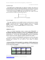
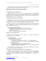
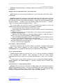
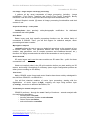
I JORNADAS DE SIG LIBRE
Introducción a los conceptos y a la utilización del
SIG Open-Source GRASS.
E. Rousseau (1)
(1) GRASS Users Community, GRASS French Translations Team [email protected]
RESUMEN
En este informe, queremos presentar el SIG GRASS (en sus versiones 5.x
y 6.x), uno de los SIG más antiguos desarrollado en la Comunidad Open
Source. El objetivo perseguido se resume explicando a cualquier utilizador
de SIG las especificaciones conceptuales de GRASS.
Después de unas consideraciones técnicas a propósito de :
– a) la utilización de GRASS en varios sistemas tales como Unix/Linux,
Windows (con Cygwin o sin), y MacOSX,
– b) la elección de una interfaz gráfica (la clásica Tcl/Tk, QGIS o
JGRASS),
– c) las interacciones funcionales entre GRASS y otros proyectos OpenSource como GDAL/OGR, Proj4, o PostgreSQL,
describiremos un primer arranque típico con la creación de un base de
datos geográficos.
Primero, se tratará de la gestión de las proyecciones y sistemas de
coordenadas a través del concepto de “Location”.
Luego, de la gestión de los utilizadores y de sus autorizaciones, tales
como en el modelo Unix, de lectura/escritura en los datos con los
“Mapset(s)”.
Por fin, veremos cómo ajustar la “Region” (a la vez para el enfoque del
zoom y la resolución de los mapas) para la visualización y el proceso de
datos.
Como otros SIG Libres, por ejemplo GvSIG, parecen más populares en la
Comunidad Hispanohablante, nos detendremos en las necesidades de
traducción de las diferentes interfaces gráficas y de la documentación, y
también en los recursos disponibles para participar.
Palabras clave: base de datos geográficos, GRASS GIS, Comunidad
Hispano-hablante, gestión de utilizadores, interfaz gráfica.
Plaça Ferrater Mora 1, 17071 Girona
Tel. 972 41 80 39, Fax. 972 41 82 30
[email protected] http://www.sigte.udg.es/jornadassiglibre/
Servicio de Sistemas de Información Geográfica y Teledetección
I Jornadas de SIG Libre
ABSTRACT
In this presentation, we would like to focus on GRASS GIS (version 5.x
and the latest 6.x), one of the oldest GIS developped by the Open-Source
Community. Our goal is trying to make it accessible to any GIS user by
explaining its main concepts.
After a couple of technical considerations on :
– using GRASS on various operating systems such as Unix/Linux,
Windows (with or without Cygwin) or MacOsX,
–
on the choice among the differents graphical interfaces available (the
classical Tcl/Tk, QGIS, JGrass),
– and on its connection with other open-source projects such as
GDAL/OGR, Proj4 or PostgreSQL,
we will describe a typical first launch and the creation of a geographic
database.
First, we will detail the management of the projection and coordinate
systems of data through the “Location”.
Then, we will review the management of users and read-write permissions
(Unix-like) within “Mapset(s)”.
Finally, we will explain the original concept of “Region” to cope with the
focus and resolution of data layers both for visualisation and data
processing.
Considering that other Free GIS, for instance GvSIG, might be more
popular and deeply rooted in Spanish-speaking countries, we will discuss
the needs of GRASS user community regarding translation of various
interfaces and documentation, and the tools presently available to
contribute.
Key words: geographical database, graphical interface, GRASS GIS,
Spanish-speaking community, users management.
INTRODUCTION
With its last version 6.x, GRASS (which stands for Geographic Resources Analysis
Support System) can fully compete with other commercial GIS softwares. Indeed, the
original GRASS 5 raster and image processing functionalities are completed with a
new vectorial engine.
Also, integration with other OpenSource softwares and libraries like :
– GDAL, for raster files import/export,
– OGR, for vector files import/export,
– PostgreSQL
and its module PostGIS for relational and spatial database
management,
– and portable and modular interfaces JGRASS (written in Java) or QGIS (written in
Qt), etc.
made GRASS a more mature and “user-friendly” GIS software.
With the help of pre-compiled GRASS binaries for various Linux distributions
(c.f. Debian GIS/Ubuntu GIS projects, but also packages for Suse, Mandriva, Fedora)
or with the long-awaited QGIS 0.8 'Titan' which includes GRASS GIS functionnalities
(vector and raster processing, GDAL and OGR import/export...), it is now much easier
Plaça Ferrater Mora 1, 17071 Girona
Tel. 972 41 80 39, Fax. 972 41 82 30
[email protected] http://www.sigte.udg.es/jornadassiglibre/
Servicio de Sistemas de Información Geográfica y Teledetección
I Jornadas de SIG Libre
to get it running properly. However, beginners remain puzzled by a couple of specific
GRASS concepts. These main concepts are : the geographical database, the
Location, the region and the mapset. In what follows, we will try to guide you through a
first start with GRASS.
Definition and practical use of GRASS main concepts
These concepts should be useful if you are launching GRASS 5.x or 6.x for the first
time in its classical configuration (“classical” meaning GRASS Tk interface under Linux
or Cygwin for instance) or if you are opening a GRASS session within QGIS 0.8.
You will be prompted with questions regarding the database, Location, region and
mapset : GRASS GIS needs you to define those parameters before you can proceed
with data integration, visualization or processing.
Creating a GRASS Geographical Database
After installing GRASS, you will need to create an empty directory on your hard disk
to store your Geographical Database and work upon them with GRASS. Usually, it is
called “grassdata” or “gisdata”.
Remember not to put any accents, tildes or spaces in the directories or files names.
For a first start, you could unzip Spearfish Database (freely downloadable on GRASS
website) in this directory. (Spearfish is a Geographical Database centered on a
national park in South Dakota, made world-famous by its monument : the faces of
four American presidents carved in the rock).
The database contains vector layers (road network, rivers, etc.), raster layers (soil
map, geological map,etc.), remote sensing images to provide a full sample of
database layers processed in GRASS.
Creating a new Location
The Location stores information on layers projection and coordinate system.
Therefore, you can have a Location called “World” with data in UTM, and another
Location called “France” with data projected in Lambert Conforme Conical.
Whenever you start GRASS, you can create a new Location : either defining its
parameters step-by-step (ellipsoïd, datum, parallels, central meridian, map units
(choose between 'meters' or 'miles')) or using a shortcut, like an EPSG code.
There are four types of Locations :
1. XY Location : for raw data (raw remote-sensing data, medical data...)
2. Latitude-Longitude Location
3. UTM Location
4. Location with other types of projections (like Laborde, Lambert, and many
others...)
Creating a new region
In GRASS, what is displayed in the map monitor strictly matches what will be
processed. Therefore, it is recommended to carefully define the default region, and to
modify it while working on maps whenever needed (for instance, you can slightly lower
the resolution of images to speed up algorithms on raster maps and images).
Plaça Ferrater Mora 1, 17071 Girona
Tel. 972 41 80 39, Fax. 972 41 82 30
[email protected] http://www.sigte.udg.es/jornadassiglibre/
Servicio de Sistemas de Información Geográfica y Teledetección
I Jornadas de SIG Libre
The default region
The default region is defined when you create the Location. The region is a
rectangle with North, South, East and West coordinates : if you are not sure, use one
of your map layers to configure it (the one with most extent is convenient) – see below
on how to proceed, then use g.region -p to know the parameters of your region.
If you fill new coordinates, always make sure that North has a bigger value than
South and East has a bigger value than West [Figura 1].
Figure 1: Region extent and NSWE coordinates
The current region
The region parameters can be modified whenever needed using the command
g.region. The region extent and resolution can match the extent of any map layer
g.region rast=my_raster_10m ; g.region rast3D=my_3d_raster ; g.region
vect=streets_vector, or mapset g.region mapset=low_resolution_mapset.
Creating a mapset
PERMANENTs mapsets
First of all, GRASS automatically creates a mapset called PERMANENT : it
contains layer maps with read permissions for any user, and write permissions only for
the database administrator. Generally, we store in the PERMANENT mapset the
original data to be processed like Numerical Data Models, remote-sensing images,
ground data truth... You can create many PERMANENT mapsets just by writing their
names in capital letters (SPOT_IMAGES, LANDSAT_IMAGES, ANY_NAME...)
It is useful to create several PERMANENTs mapsets when you have raster layers
with different resolutions because each mapset holds its own region definition
(including raster resolution), you can choose for each mapset an adequate
configuration.
You can manage read/write permissions on mapsets in GRASS exactly like on
UNIX directories [Tabla 1] : the data within a personal mapset can be completly private
(read/write permissions for you only), or available for a group, etc. These permissions
can be modified using g.mapset.
Table 1: examples of permission granting on different mapsets
Groups of Ciudad
users Girona
Mapsets
de Ciudad
de C.A.
de
Barcelona
Catalunya
Girona
Read/Write
Read
Read/Write
Barcelona
Read
Read/Write
Read/Write
Catalunya
Read
Read
Read/Write
Plaça Ferrater Mora 1, 17071 Girona
Tel. 972 41 80 39, Fax. 972 41 82 30
[email protected] http://www.sigte.udg.es/jornadassiglibre/
Servicio de Sistemas de Información Geográfica y Teledetección
I Jornadas de SIG Libre
With Location, default region and mapset(s) clearly defined, you can start building
up your GRASS project and working on your data layers.
GRASS functionnalities through several modules
Using GRASS shell and calling for help...
GRASS manual is actually the one and only official source for using GRASS
commands, even if there are many tutorials available [1][2] and/or redistributable
under GNU Free Documentation License [3]. There is one user manual for every
GRASS version : 5.4, 5.7, 6.0, and so on...
Calling GRASS manual (web browser display)
Depending on the interface you are using, you might call the manual from the menu
(in GIS Manager, i.e. the “classical” interface), or from the tab “Manual” of GRASS
ToolBox (for every command available within QGIS 0.8 GRASS Toolbox).
Anyway, in all cases, you can access manual pages directly by typing in GRASS
shell g.manual bar.foo.bone. GRASS automatically launches a web browser to
display man page in html format.
This help page provides details on :
– command use with the different flags and options available,
– an extended description of the context of use of the command,
– very often, examples of use,
– authors of the module and date of last update.
Calling concise help (within Shell)
You can also call concise help for any command : contents are displayed in
GRASS shell bar.foo.bone -help.
Concise help includes :
– a short description of the command,
– the correct way to use it where :
– flags should be typed with a minus sign (“-”), for instance d.rast -o,
– non-optional parameters are presented without brackets, like d.rast
map=a_raster_map,
– optional parameters are presented with brackets,
– parameters where the input can be a list of values, and the separator
(for instance, commas or semi-colons).
The meaning of these different options, with possible restrictions (for instance,
raster size limitation on various operations).
G for GRASS : general tasks regarding users and data management
GRASS general commands are needed to change the current mapset (g.mapset)
or the current region (g.region), and also to modify data layers, renaming them
(g.rename old_name new_name), copying them (g.copy) or
dumping them
(g.remove).
Plaça Ferrater Mora 1, 17071 Girona
Tel. 972 41 80 39, Fax. 972 41 82 30
[email protected] http://www.sigte.udg.es/jornadassiglibre/
Servicio de Sistemas de Información Geográfica y Teledetección
I Jornadas de SIG Libre
g.access command allows to manage read/write permissions for users or groups
on mapsets.
Getting a list of available data layers : g.list and g.mlist
g.list allows you to know layers available for a given data type (like raster, vector,
or raster3D).
g.mlist is designed to search for a text pattern (like part of a layer name) or to use
a regular expression to list available map layers. Like usual, the character * stands for
the unknown part of the layer name, for instance : NikoR* for any layer beginning with
the string “NikoR...”, *Landsat for all layer names ending with the string “...Landsat”,
*1995* for all layer names including the string “...1995...”.
We cannot stress too much the need to normalize layer names so that any
database user might run these queries. Normalization could be :
– not using accents, tildes, or spaces in the layer name,
– clearly stating, as an abbreviation, the type of satellite used for remote-sensing
images (i.e. Spot1),
– adding as the name (or the initial letters of the name) of the cartographer for
analysis or synthesis layers,
– indicating the date when the data was initially created, at least the year of
creation, or a more precise timestamp (AAMMJJ-HHMM),
– using normalized geographical names, for instance only local spellings of the
toponyms, or only English transpositions of the toponyms,
– using capital letters or normal letters to clearly distinguish between finalized
data layers and work-in-progress layers,
of course, these are only suggestions.
D for Display : display commands
Commands beginning with d. gather display commands : including raster layers
(d.rast), vector layers (d.vect), but also barscales (d.barscale), histograms
(d.histogram) or any graphical object that can be added on the map display.
d.mon : manage monitors
GRASS monitors (there are seven of them : x0, x1...x6) are a peculiarity of GRASS
5 and GRASS6 tcl/tk interface. Their advantage is that you might display
simultaneously various 'views' on your data (selected layers, zoom level, resolution,
etc.)
To start, select, or stop these monitors, you will use respectively d.mon start=x2,
d.mon select=x1 and d.mon stop=x6. If needed, monitors can be resized using
d.monsize.
PS for PostScript : a map-publishing module
ps.map is the one and only command in the ps.* family, but it includes the classical
GRASS map-publishing module. You can feed GRASS shell scripts (made of several
GRASS display command lines) through this command to semi-automize map
production. Examples of such scripts can be found in GRASS manuals.
Plaça Ferrater Mora 1, 17071 Girona
Tel. 972 41 80 39, Fax. 972 41 82 30
[email protected] http://www.sigte.udg.es/jornadassiglibre/
Servicio de Sistemas de Información Geográfica y Teledetección
I Jornadas de SIG Libre
I for Image : image analysis and image processing
i. gathers all the usual commands of image processing, including : image
rectification, Fast Fourier Transform and Inverse Fast Fourier Transform, Brovey
transform, PCA and CCA, supervised and non-supervised classification, etc.
Michael Shapiro's tutorial [4] states all image processing functionalities and their
context of use.
A special sub-family : i.ortho.photo
i.ortho.photo aims precisely ortho-photographic rectification. Its dedicated
commands start with i.photo.
R for Raster
Raster layers and their specific processing functions are the widest family of
commands in GRASS. There, you will find support for statistical analysis, raster
processing and raster creation.
Map algebra r.mapcalc
r.mapcalc allows the user to carry on algebrical operations on the contents of one
or several raster layers. This particular module has many functionalities (masks
creation, map generation, use of complex operators and conditional clauses, etc.),
therefore it is highly recommended to read its documentation to use it properly.
R3 for Raster3D
3D raster layers won't use the same modules as 2D raster files : prefix for these
commands is r3.
Watch out carefully what is the 3D grid resolution before you start working on 3D
rasters, and modify it accordingly if necessary (same region configuration problem as
when you are working on 2D rasters).
V for Vector
Native GRASS vector format and vector libraries have been entirely redesigned in
the shift from GRASS 5.x to GRASS 6.x.
You will find classical modules of vector layer processing, starting with the
digitalization of vector layers (v.digit), cropping one layer using another layer
(v.overlay), connexion to attribute data tables, etc.
A sub-family for network analysis v.net.*
GRASS 6 performs - through the v.net.* family of functions – network analysis with
four well-known algorithms :
• shortest path v.net.path
• traveling salesman problem v.net.salesman
• Steiner tree v.net.steiner
• sub-net allocation v.net.alloc
Plaça Ferrater Mora 1, 17071 Girona
Tel. 972 41 80 39, Fax. 972 41 82 30
[email protected] http://www.sigte.udg.es/jornadassiglibre/
Servicio de Sistemas de Información Geográfica y Teledetección
I Jornadas de SIG Libre
D for Database (Relational Databases)
db. prefix stands for management of relational databases, for instance to check
available drivers, to connect to a database, to check the structure of the databases or
of the tables, and to modify this structure (only if you have root permissions on this
database).
Running SQL queries : db.execute
db.execute allows you to execute any SQL query within GRASS (SELECT,
UPDATE, ALTER, DROP,...) You can store these queries in a text file to call them
back later easily.
These functions are only a small part of GRASS GIS capabilities, new users are
likely to try some of these functions while familiarizing themselves with the interface
and the data.
CONCLUSION
GRASS interfaces and functions have been slightly changing from GRASS 5.x to
GRASS 6.x. However, GRASS core and base concepts mostly remained the same
and are known to be the biggest obstacle for beginners.
Other steps are still needed to make GRASS more accessible and a more mainstream GIS software :
– the i18n project consists in translating GRASS messages and tk interface to
various widely-spoken languages,
– the redaction and translation of documentation, tutorials and GRASS 6.x official
manual.
Through OSGeo, Free GIS projects are now aiming towards cross-fertilization
between developers teams and organisation of translators and users through local
chapters.
ACKNOWLEDGEMENTS
The author wishes to thank Suzanne, LJ, Lud, Jérome, AMP, Y. for their advice and
ideas, and all the Faux-Rhum team for its good humour...
REFERENCES
♦ ALONSO SARRIA F.(2000), Tutorial de introduccion a GRASS, 120pp.
♦ NETELER M. (traducido por MARTINEZ G.) (2005), “GRASS 6 : una guia de
inicio”. OpenSource Geospatial '05 Conference, Junio 16-18 2005, University of
Minnesota, Minneapolis, USA.
♦ NETELER M., DASSAU O.,HOLL S., REDSLOB M. (2006), GRASS Tutorial 1.2,
GDF Hannover, 170pp.
♦ SHAPIRO M., HARMON V. (1995) GRASS Tutorial : Image Processing U.S.Army
Construction Engineering Research Laboratory, 47pp.
Plaça Ferrater Mora 1, 17071 Girona
Tel. 972 41 80 39, Fax. 972 41 82 30
[email protected] http://www.sigte.udg.es/jornadassiglibre/