No category

Download Manual for Powder Indexing Software Conograph

Transcript

Manual for Powder Indexing Software
Conograph
Oct 2015
Contents
1.
Overall configuration ...............................................................................................................1-1
2.
Creating new project/opening existing project ..........................................................................2-1
2.1.
Creating a new project ..................................................................................................... 2-1
2.2.
Opening a project ............................................................................................................. 2-5
3.
Peak search ..............................................................................................................................3-1
3.1.
Peak search execution ...................................................................................................... 3-1
3.2.
Checking peak search results ............................................................................................ 3-3
3.3.
Removing and adding peaks manually ............................................................................. 3-4
4.
Parameters used for indexing ...................................................................................................4-1
4.1.
Search parameters and diffractometer parameters ............................................................. 4-2
4.2.
Advanced indexing parameters......................................................................................... 4-5
5.
Indexing...................................................................................................................................5-1
5.1.
Indexing execution ........................................................................................................... 5-1
5.2.
When indexing is complete .............................................................................................. 5-2
5.3.
Sorting /filtering lattice parameters .................................................................................. 5-3
5.4.
Find plausible indexing solutions ..................................................................................... 5-6
5.5.
Decide the correct lattice parameters .............................................................................. 5-10
6.
Refining lattice parameters and zero point shift ........................................................................6-1
6.1.
6.1.1.
Refinement of lattice parameters selected from the list .............................................. 6-1
6.1.2.
Refining lattice constants entered by user.................................................................. 6-3
6.2.
7.
Method for refinement execution ..................................................................................... 6-1
Undo button..................................................................................................................... 6-5
Result output ............................................................................................................................7-1
7.1.
*.index.xml ...................................................................................................................... 7-1
7.2.
Igor text file and *.index2.xml file ................................................................................... 7-1
7.3.
Backup file....................................................................................................................... 7-2
8.
Space group determination .......................................................................................................8-1
9.
Other GUI operations ...............................................................................................................9-1
9.1.
Configuration parameters ................................................................................................. 9-1
9.2.
Help menu ....................................................................................................................... 9-1
10.
Parameters that can be changed to obtain better results .......................................................10-1
10.1. Peak search .................................................................................................................... 10-1
10.2. Powder indexing ............................................................................................................ 10-3
10.2.1. Conduct a more exhaustive search .......................................................................... 10-3
10.2.2. Enhance computing speed ....................................................................................... 10-3
10.2.3. Improve the efficacy of figures of merit .................................................................. 10-4
11.
Input/output text file formats............................................................................................... 11-1
12.
Addendum ..........................................................................................................................12-1
12.1. Request for citation ........................................................................................................ 12-1
12.2. Bug report ...................................................................................................................... 12-1
Acknowledgments
We would like to express our gratitude to the professors of Ibaraki University, Tokyo Institute of
Technology, and the High Energy Accelerator Research Organization for providing powder diffraction
data for this project. We would also like to thank the staff of the Visible Information Center, Inc. for
their cooperation in developing the GUI. This software was developed with the support of the
Grant-in-Aid for Young Scientists (B) (No. 22740077) and funding from Ibaraki Prefecture
(J-PARC-23D06).
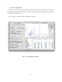
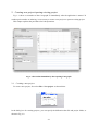
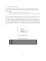
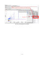
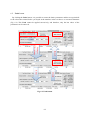
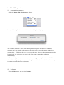
1. Overall configuration
Conograph was developed by the High Energy Accelerator Research Organization for running two
command-user-interface (CUI) programs for powder indexing and peak searching through operations
on a graphical user interface.
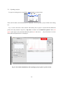
Fig. 1-1 shows a screenshot of the Conograph user interface.
Fig. 1-1 Conograph user interface
1-1
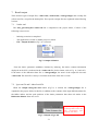
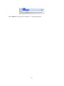
2. Creating new project/opening existing project
Fig. 1-1 shows a screenshot of the Conograph UI immediately after the application is started. To
conduct peak searches or indexing, it is necessary to create a new project or open an existing project.
This chapter explains the procedures for both operations.
Fig. 2-1 Screenshot immediately after opening Conograph
2.1. Creating a new project
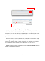
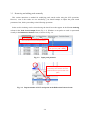
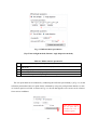
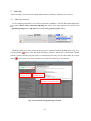
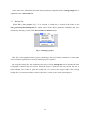
To create a new project, first select File > New project as shown below.
In the dialog box for creating projects, you can specify the diffraction data file and project folder, as
shown in Fig. 2-2.
2-1
Select diffraction data file
As the project folder, a folder containing diffraction
data is inputted automatically. This setting can be
changed if necessary.
Fig. 2-2 Dialog box for creating new project
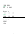
The diffraction data file can be formatted in three types of format: XY (Fig. 2-3), IGOR (Fig. 2-4),
and Rietan (Fig. 2-5). For the XY and IGOR formats, the observation errors of y-values (in the second
column) can be input in the third data column. If the third column is empty, the roots of the y-values
are used as the observation errors. In the file, LF, CR+LF, and CR can be used as a line feed code, and
spaces and tabs as a delimiter.
The project is created by clicking the OK button after providing the project information. A folder
named auto_generated_files is created in the project folder, and used to store all the automatically
outputted files. This folder contains all the files necessary for using Conograph. Thus, it contains a
copy of the diffraction data file specified in Fig. 2-2 and parameter set up files (Fig. 11-1—).
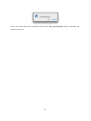
When the specified project folder already exists and contains the auto_generated_files folder as a
subfolder, the following dialog box appears:
2-2
If you select Yes, all the files originally present in the auto_generated_files folder are deleted and
cannot be retrieved.
2-3
tof
yint
7.00000 4942
7.01697 4956
7.03395 5084
～omitted～
89.66605
89.68303
89.70000
yerr
70.29935988
70.39886363
71.30217388
818
818
818
28.60069929
28.60069929
28.60069929
Fig. 2-3
IGOR
WAVES/Otof,yint,yerr
BEGIN
8792.00000
0.85962
8808.00000
0.79276
8824.00000
0.75064
～omitted～
199536.00000
0.40015
199664.00000
0.36920
199792.00000
0.39202
END
Example of XY format
0.05899
0.05643
0.05470
0.01698
0.01634
0.01686
Fig. 2-4
Example of IGOR format
Fig. 2-5
Example of Rietan format
3500
10.00000.0200
15,16,26,19
30,15,23,22
26,25,20,17
～omitted～
8,12,4,9
13,12,8,6
7,6,11,1
2-4
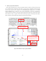
2.2. Opening a project
To open an existing project, select File > Open project as shown below.
Then, the file folder selection dialog box is displayed. You can specify a project folder in the dialog
box.
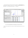
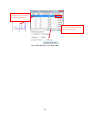
Fig. 2-3 shows the status of the software immediately after a project is opened and the diffraction
pattern file and parameter setup file (*.inp.xml) are loaded. In the Diffraction pattern frame (red
square in the figure), the measured diffraction pattern (…) and errors (―, only when there is an error
in the diffraction pattern file) are displayed.
Fig. 2-6 Screenshot immediately after opening a project (prior to peak search)
2-5
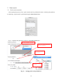
If a peak search has been performed in the opened project and the file *_pks.histogramIgor exists,
the indexing frame is displayed, as shown in Fig. 2-7. In addition to the diffraction pattern (…), the
peak positions (▲) and a smoothed diffraction pattern (―) are displayed.
Fig. 2-7 Screenshot immediately after opening a project (after peak search)
Further, when a backup file exists, the project is opened, loading indexing results saved in the
backup file.
2-6
3. Peak search
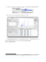
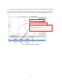
3.1. Peak search execution
After opening the project, first, a peak search must be performed in order to obtain peak positions
for indexing. A peak search is performed using the Peak search frame:
Fig. 3-1 explains the operations available in the Peak search frame.
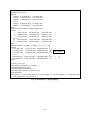
Enter an odd number (5 or more)
A new row is inserted immediately
above the selected row
MAX means an upper
limit is not set
Select a wavelength
from list
Fig. 3-1
Setting peak search parameters
3-1
To conduct a peak search, click the Run button
or select Menu > Run > Run peak search:
When the peak search is completed, the screen appears as follows.
In the Diffraction Pattern frame, a smoothed diffraction pattern (―) and peak positions (▲) are
displayed. Simultaneously, they are stored in the file auto_generated_files
folder/*_pks.hstogramIgor1.
If the peak search results found at the end of the *_pks.histogramIgor file (Fig. 11-4) are modified
using a text editor, the results are loaded on the application when the same project is reopened.
3-2
1
3.2. Checking peak search results
To obtain appropriate peak search results for indexing, you should check whether the following
problems occur, in particular, for the low-angle peaks, by magnifying the graphical display of the
diffraction pattern:
ž
Are there many diffraction peaks that have not been detected?
ž
Has noise (including small peaks that may not be diffraction peaks) been detected as a peak?
The aforementioned problems during peak search can be resolved by adjusting some of the peak
search parameters and re-executing peak search (for parameter adjustment, refer to Section 10.1).
The graph magnification in the Diffraction Pattern frame is changed by using the mouse wheel or
rubber band (= rectangular range) selection using left drag. A parallel shift of the display area is
achieved by using Ctrl + left drag or center drag. The shortcut menu that appears when you
right-click on the graph is shown in Fig. 3-2. Its components and their descriptions are listed in Table
3-1.
②
①
④
Fig. 3-2 Shortcut menu
Table 3-1 Shortcut menu
①
②
③
④
Adjusts scale to fit entire graph
Returns to the previous display status
Copies graph contents onto the clipboard
Saves graph contents in an image file
3-3
③
3.3. Removing and adding peaks manually
This section introduces a method for modifying peak search results using the GUI operations.
However, even if the results are not satisfactory, you should attempt to adjust the peak search
parameters first, before proceeding to the following operations.
Peaks used in indexing can be selected using the check boxes that appear in the Use for indexing
column in the Peak Search Output frame (Fig. 3-3). Whether or not peaks are used is represented
visually in the Diffraction Pattern frame, as shown in Fig. 3-4.
Click to switch the order (ascending/descending)
Data can be selected by dragging
and copied using Ctrl + clicking
Fig. 3-3
Input peak positions
Marker displays switches by
interlocking with ON/OFF check box
(outlined markers represent NOT used
peaks)
Fig. 3-4
Representation of NOT used peaks in the Diffraction Pattern frame
3-4
A peak can be inserted manually at the mouse pointer position by double-clicking on the diffraction
pattern. Its height is automatically decided by interpolation. The specific values of the peak position
and the full width at half maximum (FWHM) can be edited in the Peak Search Output frame (Fig.
3-5).
① Double-click on the screen,
② Peak is inserted at the mouse position
③ Peak is inserted according to its position and highlighted.
・FWHM becomes the same as the value of nearest peak.
・Parameters of peaks can be edited.
・To delete, select entire row and press Delete key.
Fig. 3-5 Manual insertion of a peak
3-5
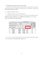
4. Parameters used for indexing
The parameters used in indexing are located in three frames (Fig. 4-1):
1.
Indexing frame
a. Search parameters and diffractometer parameters
b. Sorting criteria and thresholds for lattice parameters displayed in the list (can be
changed after indexing)
2.
Advanced indexing parameters frame
3.
Peak Search Output frame
Immediately after a new project is created, the values recommended for the respective parameters
are set. Basically, it is not necessary to change the values, except for the diffractometer parameters.
The parameter in item 3 above is introduced in Section 3.3. The criteria and thresholds in item 1b
are introduced in Section 5.3, because they can be changed even after indexing. In the current section,
the remaining two types of parameters are explained.
2.
1.
3.
These parameters are used for indexing
Fig. 4-1 Input parameters of powder indexing
4-1
4.1. Search parameters and diffractometer parameters
In the Search parameters area, the search method and number of peaks used for powder indexing
can be specified. There are two search method options:
ž
Quick search (when the size of the unit cell is small or for cases with high symmetry),
ž
Exhaustive search (for all cases)
Fig. 4-2 Search parameters
Since the basic algorithms of the two search methods are the same, the two methods can return the
same result, if you adjust the parameters used for the quick search.
Powder indexing with Quick search is successful in many cases. However, Memory-efficient
search should be used in more difficult cases. Powder indexing with Memory-efficient search
occasionally takes more than 10 minutes.
In the Diffractometer parameters area, the time-of-flight or angle dispersion method can be
selected. Except for the zero point shift, the parameter values are unique to the respective
diffractometer (Fig. 4-3, Fig. 4-4, and Table 4-1). Entering 0 deg. for the zero point shift is normally
effective. More precise values can be estimated by executing refinement after indexing.
4-2
①
②
①
③
④
⑤
Fig. 4-3 Diffractometer parameters
(Top: Time-of-flight method; Bottom: Angle dispersion method)
①
②
③
④
⑤
Table 4-1 Diffractometer parameters
Selects “Time-of-flight” or “Angle dispersion”
Conversion parameters represented as polynomial coefficients from zero
fifth order
Wavelength [Å]
Peak shift parameter ∆2q [degrees]
Estimates zero point shift by using the reflection pair method
to
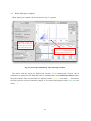
The zero point shift can be estimated by conducting the reflection pair method [1] (Fig. 4-3). In the
reflection point method, the zero point shift is estimated by using two peak positions that have a ratio
of d-values equal to two-fold. As shown in Fig. 4-3, the one that appears to be correct can be selected
from various candidates.
When button is clicked,
the zero point shift is
estimated and a list of
candidates appears.
4-3
If one of the estimated values
is selected, two peaks used for
estimation are highlighted.
When one of the estimated values
is selected and OK is clicked, the
selected value is entered.
Fig. 4-4 Estimation of zero point shift
4-4
4.2. Advanced indexing parameters
The recommended values for the parameters in this frame are set automatically when a project is
created. Although in general the values need not be changed, it should be noted that when they were
determined the most difficult cases of powder indexing were considered. Hence, improvement,
particularly in computation time, may be obtained by changing these parameters, as described in
Section 10.2.
①
②
③
④
⑤
⑨
⑥
⑦
⑧
Fig. 4-5 Advanced indexing parameters
A description of the parameters and their recommended values are listed in Table 4-2.
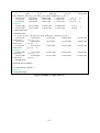
Table 4-2 Advanced indexing parameters
Contents
①
②
③
④
⑤
⑥
⑦
⑧
⑨
Recommended
value
Lower and upper limit of primitive cell volume
AUTO
2
Maximum value from four q values (= 1/d ) (q1, q2, q3, q4) acquired from AUTO
selected topography that satisfies Ito equation
Maximum number of powder indexing solutions to be enumerated (before AUTO
Bravais lattice determination)
Reference value to determine whether linear sum of q (= 1/d2) value is equal 1.0
to zero, including Ito formula
Lower thresholds for the Wu FOM (MWu), the reversed FOM (MRev), and the 1.9
distance between two closest points in the crystal lattice. If a solution has
1.0
values below these thresholds, it is deleted, and cannot be retrieved after
2.0
indexing is executed.
If a solution has a rank below this number when all the solutions with the 1000
same Bravais types are sorted in the order of the de Wolff FOM (M), it is
deleted, and cannot be retrieved after indexing is executed.
Untick the checkbox, if lattice parameter candidates of the Bravais type are ☑(Yes)
NOT necessary.
4-5
5. Indexing
After executing a peak search and setting diffractometer parameters, indexing can be started.
5.1. Indexing execution
To start indexing and obtain a list of lattice parameter candidates, click the “Run indexing” button
, or select Menu > Run > Run auto-indexing (the values of the input parameter are stored in the
*_pks.histogramIgor and *.inp.xml files from the auto_generated_files folder):
While the indexing is being executed, the progress is outputted in the Log Note frame (Fig. 5-1).
The Skip button
can be used only when searching a solution, and when it is clicked, the solution
search is aborted and the program shifts to subsequent processing. On the other hand, the Cancel
button
can be used at any time, and when it is clicked, the indexing is discontinued.
Button to cut short
indexing search
Button to abort
indexing search
Progress of indexing search is
displayed in the Log Note frame
Fig. 5-1 Screenshot during indexing execution
5-1
5.2. When indexing is complete
When indexing is complete, the screen shown in Fig. 5-2 appears.
Information about the
lattice with the largest de
Wolff FOM and lattices
of the same Bravais types
Peak positions of selected lattice
(light green｜) and peak positions
used for refinement (dark green｜)
Fig. 5-2 Screenshot immediately after indexing execution
The lattice with the largest de Wolff FOM (Section 5.3) is automatically selected, and its
information is displayed in the “Selected Lattice Constants” frame. In the Diffraction Pattern frame,
the peak positions of the selected lattice are displayed with a light green tick mark (｜). From these,
the peak positions used for refinement (Chapter 6) are selected and displayed with a dark green tick
mark (｜).
5-2
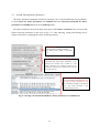
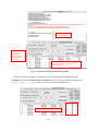
5.3. Sorting /filtering lattice parameters
The lattice parameter candidates obtained by indexing can be sorted and filtered using parameters
in the Criteria for lattice parameters in candidate list and Advanced thresholds for lattice
parameters in candidate list areas of the Indexing frame.
The lattice parameters listed in the drop-down menu of the Lattice Constants frame are sorted and
filtered using the parameters in the areas of Fig. 5-3. After indexing, sorting and filtering can be
redone at any time, by changing the values of these parameters.
①
②
③
④
⑤
Sorting criteria
Sorting criteria for lattice parameters.
For details, refer to Table 5-1 and Table
5-2.
Criteria for lattice constants displayed in list
Thresholds that limit lattice parameters to be
displayed. For details, refer to Table 5-1. The
lattice parameters are re-filtered whenever the
Enter key is pressed or the mouse cursor is moved
to another text box.
List of powder indexing solutions
Lattice parameters that satisfy “Criteria
for lattice constants displayed in list”
are classified according to the Bravais
type, and sorted according to the
specified sorting criteria.
Fig. 5-3 Sorting criteria and thresholds for lattice parameters in candidate list
5-3
An explanation of the parameters and their recommended values are listed in Table 5-1. The
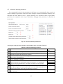
recommended values are set up automatically in the text box when a project is created.
Table 5-1 Thresholds for lattice parameters displayed in candidate list
Contents
①
②
③
④
⑤
Recommended
value
Number of n peaks used for calculation of figures of merit (FOM). (The first n 20
smallest q-values are used. This parameter can be larger than the number of
peaks contained in the diffraction pattern, because it is automatically reduced.)
If the lattice parameters are specified, it is possible to calculate the number of AUTO
peaks that exist in the range from the first to the nth observed peaks. Lower and
upper thresholds of the number.
Only lattice candidates with a de Wolff FOM (Mn) greater than this value are 3
displayed.
Lower and upper thresholds of lattice parameters a, b, c (Å).
Relative resolution of d* (= 1/d) value. (Used for deciding whether two lattices 0.03
are identical.)
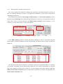
Immediately after indexing is executed, lattice parameters in the list are sorted according to the de
Wolff FOM (Mn). By using the Sorting criteria drop-down menu (Fig. 5-4), it is possible to change
the sorting criteria for the lattice parameters (refer to Table 5-2).
⑥
⑦
⑨
⑧
⑩
Fig. 5-4 Sorting criteria for lattice parameters
Among the aforementioned five FOM, the de Wolff FOM gives preference to the lattice
parameters with high symmetry, and has the best efficiency. However, another FOM occasionally
might be more effective than the de Wolff FOM, particularly if the powder diffraction pattern contains
impurity peaks [5].
The first four FOM (⑥--⑨ in Table 5-2) are defined in such a way that the values become close
to 1 if there is no correlation between the observed and computed lines. A lattice satisfying Mn > 10,
MWu > 10, MnRev > 3, or MnSym > 30 is in general likely to be the correct solution. However, sometimes
several distinct lattices may obtain large FOM values simultaneously. To select the most appropriate
lattice parameters, all the plausible solutions should be checked using the methods described in
Sections 5.4 and 5.5.
5-4
⑥
⑦
⑧
⑨
⑩
Table 5-2 Sorting criteria for lattice constants displayed in list
Sort in descending order by the de Wolff FOM (M) [6] (computed by using the method
described in [5] to increase the numerical stability). The de Wolff FOM possesses these
properties:
a) Insensitive to existence of unobserved computed lines (according to extinction rule)
b) Sensitive to existence of un-indexed observed lines (such as impurity peaks)
c) When almost identical lattices belong to different Bravais types, the lattice with higher
symmetry normally obtains a higher value.
Sort in descending order by Wu FOM (MWu) [7]. In terms of a) and b), it is similar to the de
Wolff FOM; in terms of c), it is opposite, that is, a lattice with a lower symmetry is more
likely to obtain a high value.
Sort in descending order by Reversed FOM (MRev) [5].
MRev is computed by exchanging the roles of observed peak positions and calculated peak
positions in the definition of the de Wolff FOM. Because of this, it has properties that are
opposite to those of the de Wolff FOM:
a’) Sensitive to existence of unobserved computed lines
b’) Insensitive to existence of un-indexed observed lines
c’) Tends to select a lattice with lower symmetry
As in the case of the de Wolff FOM, if there is no correlation between observed lines and
computed lines, the value becomes close to one.
Sort in descending order by Symmetric FOM (MSym = M MRev) [5]. According to its
definition, it has properties between ⑥M and ⑧ MRev. As in a number of statistical
quantities, such as chi-squares or R factors, the value remains the same after observed lines
and computed lines are exchanged
Sort in descending order by NN (=number of lattices judged to be almost identical among all
the solutions, by using the relative resolution in ⑤).
5-5
5.4. Find plausible indexing solutions
Several of the FOM introduced in Section 5.3 can extract a small number of candidates with high
compatibility with inputted peak positions from multiple powder indexing solutions. However, none
of the FOM is sufficiently effective when two lattices that belong to different Bravais types are
compared. In order not to miss plausible solutions, in addition to their values of FOM, their Bravais
types should be checked.
By using Best M Frame（Fig. 5-5）, it is possible to compare the best FOM values of the solutions
in each Bravais type. By clicking the name of a Bravais types, the solutions with the largest FOM are
displayed.
Fig. 5-5
Best M frame
Among all the lattices with
the selected Bravais type,
the candidate with the best
FOM value is displayed.
The lattice can be selected
by clicking on it.
In order not to spend much time searching for plausible solutions, you should check the
information displayed in Best M frame in terms of the following two points:
(i) Which Bravais types include a solution with a fairly large de Wolff FOM (Mn) lattice (for
5-6
example, Mn > 10)?
(ii) Among all the lattices of such a Bravais type, does the same lattice obtain the maximum value
in almost all FOM, including the de Wolff FOM? This is because different FOM have
complementary properties (refer to Table 5-2), and therefore, a lattice that has obtained the
maximum values for Mn, MnRev, and MnSym has a high possibility of being the true solution.
By clicking on a set of lattice parameters in Best M Frame (Fig. 5-5), the tick marks in the
Diffraction Pattern frame are automatically updated, and information about the parameters is
displayed in the Selected Lattice Constants frame (Fig. 5-6, Table 5-3).
①
②
③
④
⑤
⑥
Refer to Fig. 8-1
Refer to Fig. 5-12
Refer to Section 6.1.1
Fig. 5-6 Selected Lattice Constants frame
Table 5-3 Information displayed in Selected Lattice Constants frame
① Value of the de Wolff FOM (M) of the selected lattice
Wu
② Value of Wu FOM (M ) of the selected lattice
Rev
③ Value of Reversed FOM (M ) of the selected lattice
Sym
④ Value of Symmetric FOM (M ) of the selected lattice
⑤ Value of NN of the selected lattice, i.e., the number of lattices that are
found during indexing execution and judged to be identical with the
selected lattice.
3
⑥ Unit-cell volume (Å ) of the selected lattice
All the lattice parameters saved during the execution of powder indexing are displayed in Lattice
Constant Frame (Fig. 5-7）. It is possible to check peak positions of all the solutions in Lattice
Constant Frame by scrolling them, using the up and down arrow keys or the mouse wheel. By
clicking the name of a Bravais type in Lattice Constant Frame, the solution with the largest FOM
(specified in Indexing Frame) is selected:
5-7
By clicking here, the solution with the largest FOM
among solutions with the same Bravais type is selected
Scrolling using arrow keys or
mouse wheel
Fig. 5-7 List of lattice parameter candidates obtained by indexing
It should be noted that the values of the FOM are occasionally improved greatly by refinement
(Fig. 5-8). The operations necessary for refinement are explained in Section 6.1.1.
Initial value of
lattice parameters
Initial de Wolff FOM
The de Wolff FOM was improved.
Refinement is stopped if there is no further improvement
Refined lattice parameters
and zero point shift
Niggli-reduced parameters
Fig. 5-8 Message outputted in Log Note frame during refinement execution
While the refinement is being executed, a warning concerning dominant zones may appear in the
Log Note frame (Fig. 5-9). When this warning appears, it may be considered that the FOM did not
work efficiently. Therefore, it is advisable to increase the <Number of peaks used for computation of
5-8
FOM> in the Criteria for lattice constants in the list area (Fig. 5-3), according to the warning. Next
verify that there is no warning when refinement is executed again.
Warning appears that <number of peaks used for
computation of FOM> should be increased to more
than 23
Fig. 5-9 Log message reporting that a dominant zone is found
5-9
5.5. Decide the correct lattice parameters
Before drawing a conclusion as to which solution for the lattice constants is correct, the computed
lines (｜) and the observed lines (▲) should be compared. In addition, the lattice parameters may not
be determined uniquely from the peak positions (Fig. 5-10). This phenomenon occurs infrequently in
low-symmetry cases and consistently in high-symmetry cases, and is known as geometrical ambiguity
[2]. Therefore, it should be checked in respective cases whether or not the uniqueness of solutions
holds by using Conograph’s Check Uniqueness button (Fig. 5-12).
Fig. 5-10 Example of distinct lattice parameters with identical peak positions
The peak positions of all the lattices that have been refined can be displayed as tick marks on the
Diffraction Pattern frame. This allows the peak positions (｜) of several lattice parameters to be
compared simultaneously. In order to hide tick marks of some of the lattices, untick the corresponding
check boxes labeled Plot (or the corresponding lattice can be deleted) in the Stored Lattice
Parameters frame.
The methods for changing the display of tick marks are shown in Fig. 5-11 and Table 5-4.
5-10
①
②
③
④
Fig. 5-11 Diffraction Pattern frame
Table 5-4 Diffraction Pattern frame
① Displays/hides switch
② Height (y-coordinate) of the position of tick marks displayed at the top. Press
Enter key to reflect the change. This height can be increased or decreased by
locating the cursor in the text box and rotating the mouse wheel.
③ Space between tick marks and tick marks immediately below
④ Enlarges the Diffraction Pattern frame to full screen.
If the peak positions of a solution accord well with the observed lines in the diffraction patterns,
select the solution and click the Check Uniqueness button. Then, all the lattices with almost the same
peak positions as the currently selected lattice are generated [3].
If such lattices exist, a window appears as shown in Fig. 5-12. The available operations in the
window are the same as in the Diffraction Pattern frame. By clicking the “Output histogram data”
button, a histogram file that contains the peak positions of all the lattice parameters displayed is
outputted.
5-11
Fig. 5-12 Check uniqueness of solutions
5-12
6. Refining lattice parameters and zero point shift
The method for refining lattice parameter candidates obtained by indexing (and zero point shift for
angle dispersion methods) is explained in the following sections. The refinement is conducted using
linear/non-linear least squares methods.
6.1. Method for refinement execution
6.1.1. Refinement of lattice parameters selected from the list
To refine the lattice parameters and zero point shift, select the lattice parameters and then click the
Refine & store lattice constants button in the Refine Lattice Constants frame (or by selecting
Menu > Run > Refine & store lattice constants):
Fig. 6-1 shows a screenshot when the refinement is being executed. The refined lattice parameters
are saved and displayed in the Stored Lattice Constants frame.
6-1
Log reporting the
results of refinement
After refinement,
these values are
automatically
updated using the
obtained lattice
parameters.
Information here can be copied by
specifying a range by dragging and then
pressing Ctrl + C
Fig. 6-1 Screenshot during refinement execution
The peak positions to be used for refinement can be selected manually from the Use for
refinement column in the Refine lattice constants frame. The color of a tick mark changes from
dark green (|) to light green (|), according to a change in the corresponding flag.
Peaks to be used for refinement are checked
6-2
6.1.2. Refining lattice constants entered by user
This section explains the method for refining lattice parameters specified manually by the user. In
this case, although indexing execution is not required for refinement, a peak search is required for
obtaining peak positions.
The diffractometer parameter Wavelength of diffractometer (or Conversion Parameters) can be
inputted from the Indexing frame. When the angle dispersion is selected, it is also possible to enter an
initial value of the zero point shift from the Refine lattice constants frame (normally, it is not
necessary to set the initial value to a value other than 0):
If the Miller indexing button is clicked, the Miller indexing of peaks is performed using the
Bravais lattice and lattice parameters entered. Subsequently, the Miller indices assigned to peaks are
displayed:
The refinement of the lattice parameters is performed using the assigned Miller indices. If required,
it is possible to manually specify which peak positions are to be used for refinement, by using the
flags in the rightmost column (refer to Table 6-1 for the meaning of the other columns). When the
Refine & store lattice constants button is clicked, lattice parameters are refined, and appended in the
Stored Lattice Constants frame.
6-3
Table 6-1 Information about peaks in Refine lattice constants frame
Column Contents
1
Peak positions of the considered diffraction pattern
2
These values (calculated from the full widths at half maximum
of peaks) are used as weights for least squares method
3
Peak positions of the selected lattice constants computed by
using the Miller indices in column 4 and diffractometer
parameters
4
Miller indices used for refining lattice parameters
5
Checked, if the peak position is used for refining lattice
parameters
6-4
6.2. Undo button
By clicking the Undo button, it is possible to restore the lattice parameters and the zero point shift
to the values that existed before you keyed in the numbers in the text boxes or executed refinement
(Fig. 6-2). This Undo cannot be applied successively, and therefore, only the last values of the
parameters can be retrieved.
‘Undo’
Editing or
Miller indexing
‘Undo’
Refine
Fig. 6-2 Undo button
6-5
7. Result output
There are three types of output files, *.index.xml (*.index2.xml), *.histogramIgor, and a backup file
(all are text files, except for the backup file). The respective output files are explained in the following
sections.
7.1. *.index.xml
The auto_generated_files/*.index.xml file is outputted in the project folder, if either of the
following events occurs:
ž
Indexing execution is completed
ž
The application is closed or another project is started
ž
File > Output all lattices (Fig.7-1) is selected.
Fig.7-1 Output all lattices
From the lattice parameter candidates obtained by indexing, the lattice constant information
displayed on the GUI is indicated in the *.index.xml file (for the format, refer to Fig. 11-5 and 10-7).
If the name of the diffraction data file is *.histogramIgor, the name of the output file becomes
*.index.xml. The same file is always overwritten at the time of the above events.
7.2. Igor text file and *.index2.xml file
When the Output histogram data button (Fig.7-2) is clicked, the *.histogramIgor file is
outputted in the project folder. In this file, in addition to the contents of the input diffraction data file,
the Miller indices and the peak positions of the lattice parameters that show tick marks in the
Diffraction Pattern frame are saved.
Output *.histogramIgor file
containing Miller indices and
their corresponding peak
positions (tick marks)
Fig.7-2 Output of Igor file
7-1
At the same time, information about the lattice parameters outputted in the *.histogramIgor file is
outputted as the *.index2.xml file.
7.3. Backup file
When File > Save project (Fig. 7-3) is selected, a backup file is created in the folder as the
auto_generated_files/backup.dat file, which stores all the lattice parameter candidates that were
obtained by indexing or exist in the Stored Lattice Constants frame.
Fig. 7-3 Saving a project
This file is also outputted when a project containing a data set of lattice parameters is closed (this
occurs when the application is closed or another project is opened).
By using the backup file, the condition at the time of saving backup.dat can be reproduced when
Conograph is started in the next session. When the project is opened in the next session, the user is
asked whether s/he wishes to open the backup file, if it exists in the project folder. The existing
backup file is overwritten whenever either of the above events occurs in the opened project.
7-2
8. Space group determination
In the stages described thus far, only the systematic absences caused by the Bravais lattice type
were considered during computation of the figures of merit. However, additional extinction derived
from the space group may have happened. If the Determine Space Group button in the Refine
Lattice Constants frame is clicked, the value of the de Wolff figure of merit M is recomputed by
using the reflection conditions of each space group with the Bravais lattice type selected in the frame,
and a window as in Fig. 8-1 appears. The M values of all the space groups are listed up in the window,
and it is possible to check which space group fits well to the observed peaks.
Peak positions of space group
candidates are displayed.
By clicking here, information
about the space groups displayed
in the plot area is output in a
*.spgroup.xml file (Fig. 11-7) and
a *.histogramIgor file (Fig. 11-4).
Fig. 8-1 Determination of space group candidates
8-1
9. Other GUI operations
9.1. Configuration parameters
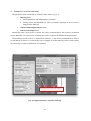
Select the Menu > File > Preferences as follows:
Then, the following Environment variables settings dialog box is displayed.
The <Number of threads> is used when running parallel computing. The number to which this
parameter can be set depends on the computer. The initial value is set to (the number of threads the
computer has) - 1. The higher the value, the greater is the speed; however, the computational cost also
becomes high. It is advisable to set a small value if you want to run another application
simultaneously.
The used configuration parameters are stored in the auto_generated_files/*.inp.xml file. The
values of the configuration parameters when the application is closed are stored in the software setup
file and are reset when the next session starts.
9.2. Help menu
From the Help menu, you can select Manuals:
9-1
When Manual is selected, the user manual (i.e., this manual) appears.
9-2
10. Parameters that can be changed to obtain better results
10.1. Peak search
In peak search, it is recommended that diffraction peaks are collected as uniformly as possible on
the basis of peak height. Filtering diffraction peaks manually (including removal of overlapped peaks)
is unnecessary and not desirable, unless there is valid prior information.
In order to obtain such a peak search result, only the following parameters need to be adjusted:
(1) <Threshold for peak height>
(2) <Number of data points used for smoothing histogram>.
In addition, in cases of characteristic X-ray data that contain a2 peaks, the a2 peaks must be
removed prior to powder indexing (Fig. 3-1).
The following are notes related to the adjustment of the parameters (1) and (2).
(1) <Threshold for peak height>
This parameter is used as a lower threshold for magnitudes of intensities to be detected in a
peak search. If c×(error value of intensity) is used, as in the default setting, a peak at
peak-position x is detected, if and only if it has a peak height greater than (the threshold) × Err[y],
where Err[y] is the value of the error in intensity at x. The peak height used here is obtained by
subtracting the estimated background value from y. Our recommended threshold value is within
the range of 3—10.
Fig. 10-1 Example of peak search results in radiation beam data
(2)
<Number of data points used for differential calculation>
This parameter can be used to avoid background noise being picked up as peaks. If it has a small
value, the smoothing curve is fit more finely to local irregularity, because the number of data points
for computing each y-value of the smoothing curve is set to this value. Fig. 10-2 shows an example.
10-1
Fig. 10-2
Fig. 10-3
<Number of data points> = 5
10-2
<Number of data points> = 25
10.2. Powder indexing
It has been confirmed that a search using the recommended parameter values provides correct
solutions in an extremely wide range of cases, in particular, in memory-efficient search [4].
Nevertheless, if good results are not obtained, they may be improved by changing some of the
parameters. In the following, the parameters to be changed in order to conduct a more exhaustive
search (Section 10.2.1), enhance computing speed (Section 10.2.2), and improve the efficacy of the
figures of merit (Section 10.2.3) are explained.
10.2.1. Conduct a more exhaustive search
(1) <Searching method> in Indexing frame: Quick search Þ Exhaustive search.
(2) <Number of peaks used in the search> (Indexing frame): AUTO Þ a number greater than 48
When AUTO is entered, 48 peaks are used for powder indexing, unless the diffraction pattern
contains only a smaller number of peaks. However, even this number of peaks may be
insufficient if a dominant zone exists. In such cases, increasing the number is effective.
(3) <Tolerance level for errors of sums of q values> (Advanced Indexing parameter frame): 1
Þ 1.5
In cases of characteristic X-rays or reactor sources, better results may be yielded if a large
value is used.
10.2.2. Enhance computing speed
(1) Increase <Number of threads> (File > Preferences)
The simplest method is to increase the number of threads used.
(2) <Search parameters> (Indexing parameters frame): Exhaustive search Þ Quick search.
(3) <Bravais lattice> (Advanced Indexing Parameters frame): untick
If you have prior information about the Bravais type, the information can be used to reduce
the time required in the stage after Bravais lattice determination.
(4) Increase values of <Volume of primitive cell> or <Thresholds of minimum distance between
lattice points> (Advanced Indexing Parameter frame)
If you have prior information about these parameters, the information can be used to reduce
the time required for powder auto-indexing.
10-3
10.2.3. Improve the efficacy of figures of merit
(1) <Zero point shift> (Indexing frame): 0 deg. ⇒ more accurately estimated value
For diffraction patterns with a large zero point shift (∆2q > approximately 0.1o), the FOM
values sometimes become small. The results may be improved by conducting powder indexing
using the estimated value of the zero point shift. The zero point shift can be estimated by using
one of the following methods.
(a) The reflection pair method [1],
(b) After conducting powder indexing once, refine the zero point shift and lattice
parameters with relatively larger MnRev and MnSym (for instance, MnRev > 3 or MnSym >
10 approximately), and re-execute indexing, using the obtained zero point shift.
In both methods, it is necessary to test several candidate values.
(2) <Number of peaks used for computation of FOM> (Indexing frame): 20 Þ a number
greater than 20
The value 20 frequently used for this parameter might be insufficient if a problem called
dominant zone occurs. If a dominant zone is found when refining the lattice constants and zero
point shift, a warning message and the number of peaks required appear in the Log Note frame.
In that case, set this parameter to a value greater than the number displayed.
(3) Improve results of peak search (or change the <Use for Indexing> flags in Peak search
output frame)
Impurity peaks greatly affect the sorting results. Because of this, it is desirable to reduce the
number of impurity peaks as far as possible, at least in the range of the first to n-th peaks, when
the parameter <Number of peaks used for computation of FOM> is set to n.
10-4
11. Input/output text file formats
The formats for the input/output text files, cntl.inp.xml, *.inp, *.histogramIgor, and *.index files,
are shown in this section.
<ZCodeParameters>
<ConographInputFile>

<ControlParamFile> HRP000675.BS.bin04f.inp.xml </ControlParamFile>

<PeakDataFile> HRP000675.BS.bin04f_pks.histogramIgor </PeakDataFile>

<OutputFile> hrp000675.bs.bin04f.index </OutputFile>
</ConographInputFile>
<PeakSearchInputFile>
<ControlParamFile> HRP000675.BS.bin04f.inp.xml </ControlParamFile>
<HistogramDataFile>
<FileName> HRP000675.BS.bin04f.histogramIgor </FileName>

<Format> IGOR </Format>

<IsErrorContained> 1 </IsErrorContained>
</HistogramDataFile>
<Outfile> HRP000675.BS.bin04f_pks.histogramIgor </Outfile>
</PeakSearchInputFile>
</ZCodeParameters>
Fig. 11-1 Example of cntl.inp.xml
11-1
<?xml version="1.0" encoding="UTF-8" ?>
<ZCodeParameters>
<ConographParameters>


<IsAngleDispersion> 0 </IsAngleDispersion>

<ConversionParameters> 0 1 0
</ConversionParameters>

<PeakShiftParameters> 0 </PeakShiftParameters>

<WaveLength> 1.54056 </WaveLength>

<SearchLevel>

</SearchLevel>
0

<MaxNumberOfPeaks> AUTO </MaxNumberOfPeaks>

<CriticalValueForLinearSum>
1 </CriticalValueForLinearSum>

<MinPrimitiveUnitCellVolume>
AUTO </MinPrimitiveUnitCellVolume>

<MaxPrimitiveUnitCellVolume>
AUTO </MaxPrimitiveUnitCellVolume>

<MaxNumberOfTwoDimTopographs> AUTO </MaxNumberOfTwoDimTopographs>

<MaxNumberOfLatticeCandidates> AUTO </MaxNumberOfLatticeCandidates>

<OutputTriclinic> 1 </OutputTriclinic>
<OutputMonoclinicP> 1 </OutputMonoclinicP>
<OutputMonoclinicB> 1 </OutputMonoclinicB>
<OutputOrthorhombicP> 1 </OutputOrthorhombicP>
<OutputOrthorhombicB> 1 </OutputOrthorhombicB>
<OutputOrthorhombicI> 1 </OutputOrthorhombicI>
<OutputOrthorhombicF> 1 </OutputOrthorhombicF>
<OutputTetragonalP> 1 </OutputTetragonalP>
<OutputTetragonalI> 1 </OutputTetragonalI>
<OutputRhombohedral> 1 </OutputRhombohedral>
<OutputHexagonal> 1 </OutputHexagonal>
<OutputCubicP> 1 </OutputCubicP>
<OutputCubicI> 1 </OutputCubicI>
<OutputCubicF> 1 </OutputCubicF>
Fig.11-2 Example of *.inp.xml (1/2)
11-2


<Resolution> 0.05 </Resolution>

<MaxNumberOfUnindexedPeaks> 20 </MaxNumberOfUnindexedPeaks>

<MaxNumberOfPeaksForFOM> 20 </MaxNumberOfPeaksForFOM>

<MinFOM> 3 </MinFOM>

<MaxNumberOfMillerIndicesInRange> AUTO </MaxNumberOfMillerIndicesInRange>
<MinNumberOfMillerIndicesInRange> AUTO </MinNumberOfMillerIndicesInRange>

<MaxUnitCellEdgeABC> 1000 </MaxUnitCellEdgeABC>
<MinUnitCellEdgeABC> 0 </MinUnitCellEdgeABC>
</ConographParameters>
<PeakSearchPSParameters>
<ParametersForSmoothingDevision>

<NumberOfPointsForSGMethod> 9 </NumberOfPointsForSGMethod>
<EndOfRegion>

MAX
</EndOfRegion>
</ParametersForSmoothingDevision>
<PeakSearchRange>
<Begin> 0.0 </Begin>
<End> MAX </End>
</PeakSearchRange>

<UseErrorData> 1 </UseErrorData>

<Threshold> 5.0 </Threshold>

<UseBGRemoved> 0 </UseBGRemoved>

<Alpha2Correction> 0 </Alpha2Correction>
<Waves>
<Kalpha1WaveLength> 1.54056 </Kalpha1WaveLength>
<Kalpha2WaveLength> 1.54439 </Kalpha2WaveLength>
</Waves>
</PeakSearchPSParameters>
</ZCodeParameters>
Fig. 11-3 Example of *.inp.xml (2/2)
11-3
IGOR
WAVES/O tof, yint, yerr
BEGIN
1850.00 2.871904E-001 3.359009E-003
1854.00 2.834581E-001 3.337111E-003
1858.00 2.848073E-001 3.351369E-003
～Omitted～
49564.0 9.989611E-002 1.378697E-002
49588.0 1.010892E-001 1.386346E-002
END
WAVES/O peak, peakpos, height, FWHM, Flag
BEGIN
1 3.148311E+003 1.535192E-001 3.749774E+001
2 3.340909E+003 1.676432E-001 2.429063E+001
3 3.697289E+003 1.661457E-001 2.063853E+001
～Omitted～
49 3.133224E+004 2.968128E+000 1.480559E+002
50 4.906641E+004 1.092195E-001 1.791403E+002
END
WAVES/O dphase_1, xphase_1, yphase_1, h_1, k_1, l_1
BEGIN
3.138130E+000 3.133851E+004 0.000000E+000
1
2.717700E+000 2.713443E+004 0.000000E+000
0
1.921704E+000 1.918059E+004 0.000000E+000
0
～omitted～
6.405680E-001 6.394727E+003 0.000000E+000
2
6.405680E-001 6.394727E+003 0.000000E+000
0
END
1
1
1
1
1
-1
1
0
2
Only output
2
-2
2
6
-8
-6
X Display yint vs tof
X AppendToGraph yphase_1 vs xphase_1
X ModifyGraph mirror(left)=2
X ModifyGraph mirror(bottom)=2
X ModifyGraph rgb(yint)=(0,65535,65535)
X ModifyGraph
offset(yphase_1)={0,0},mode(yphase_1)=3,marker(yphase_1)=10,msize(yphase_1)=3,mrkThick(ypha
se_1)=0.6,rgb(yphase_1)=(3,52428,1)
Fig. 11-4 Example of *.histogramIgor
11-4
<ConographOutput>


<SelectedLatticeCandidate number="140153">
<CrystalSystem>
Cubic(F) </CrystalSystem>

<LatticeParameters> 5.4354e+000
5.4354e+000
</LatticeParamters>
5.4354e+000
9.0000e+001
9.0000e+001

<ReciprocalLatticeParamters>
3.3848e-002
3.3848e-002
3.3848e-002
0.0000e+000
0.0000e+000 </ReciprocalLatticeParamters>

<InitialReciprocalLatticeParamters>
3.4129e-002
3.4129e-002
3.4129e-002
0.0000e+000
0.0000e+000 </InitialReciprocalLatticeParamters>
<VolumeOfUnitCell> 1.5861e+002 </VolumeOfUnitCell>
<FigureOfMeritWolff name="Fw20"> 7.6120e+000 </FigureOfMeritWolff>
<NumberOfLatticesInNeighborhood>
213 </NumberOfLatticesInNeighborhood>
9.0000e+001
0.0000e+000
0.0000e+000

<NumberOfMillerIndicesInRange> 2.7750e+001 </NumberOfMillerIndicesInRange>
<EquivalentLatticeCandidates>
<LatticeCandidate number="13034">
<CrystalSystem>
Cubic(I) </CrystalSystem>
<LatticeParamters>
4.1917e+000
4.1917e+000
4.1917e+000
9.0000e+001
9.0000e+001 </LatticeParamters>
<ReciprocalLatticeParamters>
2.8457e-002
2.8457e-002
5.6913e-002
0.0000e+000
0.0000e+000 </ReciprocalLatticeParamters>
<FigureOfMeritWolff name="Fw20"> 1.3537e+000 </FigureOfMeritWolff>
<NumberOfLatticesInNeighborhood>
213 </NumberOfLatticesInNeighborhood>
</LatticeCandidate>
～Omitted～
</EquivalentLatticeCandidates>
Fig. 11-5 Example of *.index.xml (1/2)
11-5
9.0000e+001
0.0000e+000
<IndexingResults>
<!-q_obs,
q_cal,
peak_pos,
pos_cal,
closest_hkl,
is_the_difference_between_q_obs_and_q_cal_small_compared_to_q_err?.-->
4.1501e-002
1.0154e-001
4.9066e+004
3.1339e+004
[-1,1,1]
0
1.0159e-001
1.0154e-001
3.1332e+004
3.1339e+004
[-1,-1,-1]
1
2.1784e-001
2.7079e-001
2.1387e+004
1.9181e+004
[0,-2,-2]
0
～Omitted～
2.2680e+000
2.2678e+000
6.6286e+003
6.6288e+003
[7,3,-3]
1
2.4367e+000
2.4371e+000
6.3952e+003
6.3947e+003
[-6,6,0]
1
</IndexingResults>
<FittingResults>

4.1501e-002
1.2834e-004
1.0154e-001
4.9066e+004
3.1339e+004
[-1,1,1]
0
1.0159e-001
4.0706e-004
1.0154e-001
3.1332e+004
3.1339e+004
[-1,-1,-1]
1
2.1784e-001
8.7727e-004
2.7079e-001
2.1387e+004
1.9181e+004
[0,-2,-2]
0
～omitted～
2.2680e+000
7.2533e-003
2.2678e+000
6.6286e+003
6.6288e+003
[7,3,-3]
1
2.4367e+000
8.1458e-003
2.4371e+000
6.3952e+003
6.3947e+003
[-6,6,0]
1
</FittingResults>
</SelectedLatticeCandidate>

～omitted～
</ConographOutput>
Fig.11-6 Example of *.index.xml (2/2)
11-6
1.7914e+002
1.4806e+002
1.0149e+002
2.4936e+001
2.5146e+001
<ZCodeParameters>
<ConographOutput>
<TypeOfReflectionConditions>
<Candidates>
<SpaceGroups> 45(bca),72(bca) </SpaceGroups>
<ReflectionConditions> hk0:h,k=2n,0kl:k,l=2n </ReflectionConditions>
<FigureOfMeritWolff name="M20"> 3.126279e+002 </FigureOfMeritWolff>
<IndexingResults>

1.016473e-001 9.594352e-004 1.015807e-001 3.132270e+004 1.480559e+002
3.133298e+004
[1,0,-1]
1
2.708116e-001 2.274422e-003 2.707887e-001 1.917970e+004 8.059404e+001
1.918051e+004
[0,2,0]
1
3.724714e-001 2.575261e-003 3.724523e-001 1.635279e+004 5.655483e+001
1.635321e+004
[2,1,1]
1
～Omitted～
2.539049e+000 2.019023e-002 2.539077e+000 6.265138e+003 2.488311e+001
6.265104e+003
[3,4,-5]
1
2.707958e+000 2.205347e-002 2.707998e+000 6.066813e+003 2.467594e+001
6.066769e+003
[2,6,0]
1
</IndexingResults>
</Candidates>
～Omitted～
</TypeOfReflectionConditions>
</ConographOutput>
Fig. 11-7 Example of *.out.xml
11-7
12. Addendum
12.1. Request for citation
Please cite the following when research findings obtained using Conograph are mentioned in
academic manuscripts:
R. Oishi-Tomiyasu, “Robust powder auto-indexing using many peaks”, J. Appl. Cryst., 47 (2014), pp.
593–598.
The methods and figures of merit of Conograph are also introduced in the following papers:
ž
R. Oishi-Tomiyasu, “A method to enumerate all geometrical ambiguities in powder indexing and
its application”, submitted.
ž R. Oishi-Tomiyasu, “Distribution rules of systematic absences on the Conway topograph and
their application to powder auto-indexing”, Acta Cryst. A69 (2013), pp. 603–610.
ž R. Oishi-Tomiyasu, “Reversed de Wolff figure of merit and its application to powder indexing
solutions”, J. Appl. Cryst., 46 (2013), pp.1277–1282.
ž R. Oishi-Tomiyasu, “Rapid Bravais-lattice determination algorithm for lattice parameters
containing large observation errors”, Acta Cryst. A68 (2012), pp. 525–535.
ž R. Oishi, M. Yonemura, T. Ishigaki, A. Hoshikawa, K. Mori, T. Morishima, S. Torii, T.
Kamiyama, “New approach to indexing method of powder diffraction patterns using topographs”,
Zeitschrift für Kristallographie Supplements 30 (2009), pp. 15–20.
12.2. Bug report
Please send the following information to the e-mail address [email protected]. All
comments will be considered and reflected at the time of Conograph version upgrading.
(i) OS used (including 32-bit and 64-bit)
(ii) Conograph version used (indicated in the GUI Help menu)
(iii) Particulars of problem
(iv) Details of conditions when problem occurred
(v) Possibility of recurrence (does it occur always or sometimes?)
(vi) Name, affiliation, e-mail address (to allow us to contact you)
Depending on the contents of the problem, we may request the input/output files and other
information. We seek your cooperation in this regard.
12-1
References
[1] C. Dong, F. Wu, H. Chen, Correction of zero shift in powder diffraction patterns using the
reflection-pair method, J. Appl. Cryst., 32, pp. 850–853 (1999).
[2] A. D. Mighell, A. Santoro, Geometrical Ambiguities in the Indexing of Powder Patterns, J. Appl.
Cryst., 8, pp. 372–374 (1975).
[3] R. Oishi-Tomiyasu, A method to enumerate all geometrical ambiguities in powder indexing and
its application, submitted.
[4] R. Oishi-Tomiyasu, Robust powder auto-indexing using many peaks, J. Appl. Cryst., 47 (2014),
pp. 593–598.
[5] R. Oishi-Tomiyasu, Reversed de Wolff figure of merit and its application to powder indexing
solutions, J. Appl. Cryst., 46 (2013), pp. 1277–1282.
[6] P. M. de Wolff, A simplified criterion for the reliability of a powder pattern indexing, J. Appl.
Cryst., 1, pp. 108–113 (1968).
[7] E. Wu, A modification of the de Wolff figure of merit for reliability of powder pattern indexing, J.
Appl. Cryst., 21, pp. 530–535 (1988).
12-2

Top types

Top brands

Top types

Top brands

Top types

Top brands

Top types

Top brands

Top types

Top brands

Top types

Top brands

Top types

Top brands

Top types

Top brands

Top types

Top brands

Top types

Top brands

Top types

Top brands

Top types

Top brands

Top types

Top brands

Download Manual for Powder Indexing Software Conograph