Download Interactive Power Systems Calculator

Interactive Power Systems Simulator User’s
Manual
Copyright Carnegie Mellon University
December 16, 2007
Contents
1 Introduction
3
2 Using IPSYS
2.1 Data Types . . . . . . . . . . . .
2.2 Built in Operators and Functions
2.3 Scripts and Functions . . . . . . .
2.4 Power Systems Functions . . . . .
2.5 Input/Output and Miscellaneous
Functions . . . . . . . . . . . . .
.
.
.
.
.
.
.
.
.
.
.
.
.
.
.
.
.
.
.
.
.
.
.
.
.
.
.
.
.
.
.
.
.
.
.
.
.
.
.
.
.
.
.
.
.
.
.
.
.
.
.
.
.
.
.
.
.
.
.
.
.
.
.
.
6
7
12
18
22
. . . . . . . . . . . . . . . . 27
3 Matlab Interface
29
3.1 Introduction . . . . . . . . . . . . . . . . . . . . . . . . . . . . 29
3.2 Matlab Interface Data . . . . . . . . . . . . . . . . . . . . . . 30
3.3 Matlab Interface Functions . . . . . . . . . . . . . . . . . . . . 33
4 GIPSYS Interface
35
4.1 Entering a New Network . . . . . . . . . . . . . . . . . . . . . 36
4.2 Running IPSYS Algorithms . . . . . . . . . . . . . . . . . . . 38
5 IPSYS Examples
5.1 Linear Algebra . . . . . . . . . . . . . . . . .
5.1.1 Checking Rank and Condition Number
5.1.2 Sensitivity Matrix Extraction . . . . .
5.1.3 Matrix Decomposition and Clustering .
5.2 Power Flow Examples . . . . . . . . . . . . .
5.2.1 Example 1 . . . . . . . . . . . . . . . .
5.3 DC Optimal Power Flow - Flexible Generation
5.4 DC Optimal Power Flow - Flexible Load . . .
1
.
.
.
.
.
.
.
.
.
.
.
.
.
.
.
.
.
.
.
.
.
.
.
.
.
.
.
.
.
.
.
.
.
.
.
.
.
.
.
.
.
.
.
.
.
.
.
.
.
.
.
.
.
.
.
.
.
.
.
.
.
.
.
.
.
.
.
.
.
.
.
.
40
41
41
41
42
44
44
48
53
5.5
DC Optimal Power Flow - Flexible Generation and Load . . . 55
6 Matlab Examples
58
6.1 Matlab Input Output . . . . . . . . . . . . . . . . . . . . . . . 58
6.2 Matlab Functions . . . . . . . . . . . . . . . . . . . . . . . . . 62
7 Notes, Bugs, TODO list
64
A Installation
67
B Description of the PTI Load Flow Data Format
68
C Power Flow Review
73
D Optimal Power Flow Review
77
E DC Optimal Power Flow Review
79
2
Chapter 1
Introduction
Academic research frequently suffers from programming limitations of general purpose programming languages such as Fortran, C/C++, as well as
interpreted languages such as Matlab. General programming languages provide the ultimate flexibility at the price of long development cycles and are
difficult to maintain once the access to the original developers is not available anymore. On the other hand, interpreted languages provide significant
development and maintenance flexibility at the price of programming features and frequently $ price. After surveying both approaches to scientific
programming, it seemed that it could be possible to have the best of the
both worlds, that is an interpreted language expandable with natively coded
modules and ability to call native functions from the interpreter and even
the interpreter functions from the native functions and all that for a small
price in flexibility and short learning curve. The result of this conclusion is a
generic Application Programming Interface (API) framework. Appropriate
power systems functionality is added to this framework producing Interactive
Power Systems Simulator or IPSYS for short. The framework allows adding
new special purpose modules independently of existing modules and using
the built in Command Line Interface (CLI) or develop custom Graphical User
Interface (GUI). The both of these approaches are used for a development
of a power systems simulator and their use is described in this manual along
the generic framework features.
The Interactive Power System Simulator (IPSYS) is a scripting tool used
to define, manipulate, and analyze electrical power systems described using Power Technologies, Inc. input data format as described in [4]. A user
3
can interact with a single or multiple power systems through IPSYS shell,
Matlab interface (MIPSYS), or a single network using a GUI interface (GIPSYS). IPSYS libraries can be used for developing different purpose interactive
programs using the C++ programming language. Power networks are completely modeled as objects and can be operated on through a set of message
passing methods. Separate power network objects can be interfaced by setting the power generation in one of the systems and matching load in the
adjacent system. Determining the level of power exchange can be done either
using the IPSYS shell or C++ programming. This User Manual describes
IPSYS, MIPSYS, and GIPSYS functionality; application Programming Interface (API) is described in a different manual.
IPSYS shell interface features can be grouped in four distinctive parts: data
types, general type operators and functions, program control and scripting,
and specialized power systems routines. IPSYS supports real number, matrix, and character string variables. All of these data types can be entered
interactively, with a script, or in the case of matrices from a file. Power
system networks are modeled as separate objects that can be read in from a
file, manipulated, modified, simulated, optimized, and the resulting system
can be stored in an external file. Multiple power system networks are stored
at the global scope and as such can be accessed from any built in or scripting function. General purpose operators and functions include usual arithmetic and logical operators, transcendental, and linear algebra functions.
Any other functions can be added to this set provided that the function parameters operate on available data types and the result is also an available
data type. Program flow control structures provide enough functionality for
a complete procedural programming language. This includes logical tests,
looping, and input and output functionality. User functions defined as ipsys
scripts or C++ functions are supported with input and output arguments
passed by value. From users’ perspective, there is no difference between ipsys and C++ functions. Due to the object oriented power system modeling,
data and functional encapsulation are provided by the power system objects.
Power systems functions include AC power flow, implementation of different
optimal power flow algorithms, as well as a programmatic way to manipulate
the networks being simulated. The optimization routines us commercial library (IMSL) but they could use any other commercial and non commercial
C/C++/F77 library.
4
GIPSYS adds to IPSYS a GUI interface from which a network can be entered,
modified and a few common algorithms executed. GIPSYS is a semi independent front end library developed for a different purpose and illustrates
the flexibility with which new modules with very little interdependence can
be added to the framework. The only difference between IPSYS run without
GUI and with GUI is that the GUI version does not handle more than one
network at the time.
MIPSYS is the Matlab interface to IPSYS back end routines. Since Matlab
provides much richer general computational language capabilities, the only
IPSYS routines that are exported to Matlab are the power systems specific
which are not part of Matlab. This development branch uses an older IPSYS
version and is abandoned in favor of IPSYS and GIPSYS user interfaces and
ability to export power system networks to Matlab environment.
5
Chapter 2
Using IPSYS
In this chapter, IPSYS data structures, operators, program control, and programming are discussed in detail. These are the core features that are available for power systems functions and GIPSYS use both of which are discussed
in subsequent chapters.
IPSYS CLI is started by simply typing ipsys.exe command at the command
prompt provided that the the IPSYS executable is in the systems PATH.
Exiting from IPSYS is done by typing quit command:
prompt$ ipsys
***************************************************************
Interactive Power Systems Simulator
Carnegie Mellon University
Aug 25 2007 08:49:46
***************************************************************
ipsys> quit;
prompt$
After started, IPSYS is accepting commands as described in the rest of this
manual. The following sections introduce IPSYS data types, operators, commands and includes the reference information.
6
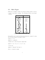
2.1
Data Types
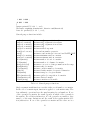
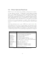
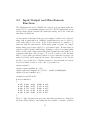
IPSYS uses real number, matrix, and character string variables as well as
a number of predefined constants,. The following is the list of predefined
constants:
Constant Symbol Constant Value
ME
e
M LOG2E
log2 (e)
M LOG10E
log10 (e)
M LN2
ln(2)
M LN10
ln(10)
M PI
π
π
M PI 2
2
π
M PI 4
4
1
M 1 PI
π
2
M 2 PI
π
√2
M 2 SQRTPI
√π
M SQRT2
q2
1
M SQRT1 2
2
RAND MAX
RAND MAX
Table 2.1: Common mathematical constants
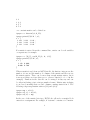
Real variables can be introduced through an interactive command or script
and follows the standard real number format:
ipsys> a = 2.5;
ipsys> b = cos(M_PI);
A matrix can be entered from the command line:
ipsys> a = [1, 2,3; 4, 5, 7; 9, 7, 4];
or from a file:
ipsys> a = Matrix(‘‘3x3.mat’’);
where 3 × 3.mat file contains:
7
3
1
4
9
3
2 3
5 7
7 4
or a constant matrix can be defined as:
ipsys> a = Matrix(3,3,M_PI);
ipsys> printf("%6.3f ",a);
a = [
3.142 3.142 3.142 ;
3.142 3.142 3.142 ;
3.142 3.142 3.142
]
If a matrix is entered from the command line, entries can be real variables
or expressions, for example:
ipsys> a = [M_PI, cos(M_PI_2); 0, 1/2];
ipsys> printf("%7.3f",a);
a = [
3.142 0.000;
0.000 0.500
]
When a matrix is read from an ASCI data file, the first two integers are the
number of rows and the number of columns of the matrix and the rest are
the matrix entries. There can be more than enough matrix entries, but it
is an error if there are fewer then rows × columns entries (3 × 3 = 9 in the
example). Numbers in the data file can be arranged in any way and can
be either in floating point or integer number format. Matrix entry indexing
is one based, meaning that row and columns counting starts from 1. The
following script swaps matrix entries a(1,1) and a(2,2):
ipsys> tmp = a(1,1);
ipsys> a(1,1) = a(2,2);
ipsys> a(2,2) = tmp;
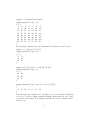
In the case of the matrix data type, IPSYS also allows for a matrix block
extraction or assignment. For example, if “test.mat” contains a 8 × 7 matrix:
8
ipsys> t = Matrix("test.mat");
ipsys> printf("% 3g ",t);
t = [
1
2
3
4
5
6
7 ;
8
9 10 11 12 13 14 ;
15 16 17 18 19 20 21 ;
22 23 24 25 26 27 28 ;
29 30 31 32 33 34 35 ;
36 37 38 39 40 41 42 ;
43 44 45 46 47 48 49 ;
50 51 52 53 54 55 56
]
the following commands show how matrix block extraction can be used:
ipsys> a = t([1,2,3],[2,3]);
ipsys> printf("% 3g ",a);
a = [
2
3 ;
9 10 ;
16 17
]
ipsys> a([1,2],[1,2]) = t([7,8],[6,7]);
ipsys> printf("% 3g ",a);
a = [
48 49 ;
55 56 ;
16 17
]
ipsys> printf("% 3g ",t(2,[1,2,3,4,5,6,7]));
[
8
9 10 11 12 13 14
]
Note that the index matrices are actually row vectors and that indexing is
one based. To index contiguous matrix elements, Range function can be used
to generate index range. For example, the first two rows of a matrix can be
extracted as:
9
ipsys> a = Matrix("shiljak.mat");
ipsys> printf("%6.3f ",a(Range(1,2),Range(1,Cols(a))));
[
0.000 0.000 0.010 0.000 2.150 0.000 0.040 0.000 ;
0.070 1.100 0.030 0.000 -0.060 -0.020 0.000 0.250
]
IPSYS provides function for construction of constant and identity matrices.
Following commands calculate the inverse of matrix a:
ipsys> a = [1,2,3;4,5,4;3,2,1];
ipsys> i = Idn(3);
ipsys> printf("% 3.2f ", i/a);
[
0.38 -0.50 0.88 ;
-1.00 1.00 -1.00 ;
0.87 -0.50 0.37
]
ipsys> printf("% 3.2f ", a*i/a);
[
1.00 -0.00 -0.00 ;
-0.00 1.00 -0.00 ;
0.00 0.00 1.00
]
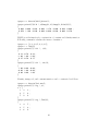
Identity, transposed, and constant matrices can be constructed as follows:
ipsys> a = Matrix("3x3.mat");
ipsys> printf("% 3.2g ",a);
a = [
1
2
3 ;
4
5
6 ;
7
8
9
]
ipsys> printf("% 3.2g ",Trn(a));
[
1
4
7 ;
2
5
8 ;
3
6
9
10
]
ipsys> printf("% 3.2g ",Idn(3));
[
1
0
0 ;
0
1
0 ;
0
0
1
]
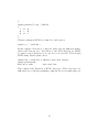
Character strings in IPSYS are defined by double quotes:
ipsys> a = ‘‘1234.234’’;
In this example, 1234.234 is a character string and any numerical manipulation will cause an error. In addition to the ASCI character set, IPSYS
recognizes escaped characters \t as a tab and \n as a new line. The following
IPSYS string variable prints out as:
ipsys> str = "Here are 2 tabs\t\t and a new line\n";
ipsys> printf(str);
Here are 2 tabs
and a new line
This completes the discussion of IPSYS data types. These data types are
sufficient for procedural programming commonly used for scientific purposes.
11
2.2
Built in Operators and Functions
IPSYS interprets the usual arithmetic operators and one argument functions
of different data types in an intuitive way. Addition, subtraction, multiplication, and division can be used with real numbers, matrices and a combination of both. The only requirement is that the matrix/matrix operations
have compatible dimensions. When a two argument operator is applied to a
real number and a matrix, the operator is applied element-wise. That is, the
operation is between the scalar and each of the matrix elements. For example:
ipsys> a = [1,2;3,4];
ipsys> printf("% 2.3f ", 1/a);
[
1.000 0.500 ;
0.333 0.250
]
ipsys> printf("% 3.3g ", 2*a*2);
a = [
4
8 ;
12 16
]
ipsys> printf("% 3.3g ", a/2);
a = [
0.5
1 ;
1.5
2
]
Examples of matrix/matrix operations:
ipsys> a = [1,2;3,4];
ipsys> b = [2,3;5,7];
ipsys> printf("% 3.3g ", a*b);
[
12 17 ;
26 37
]
ipsys> printf("% 3.3f ", (a/b)*(b/a));
[
12
1.000 0.000 ;
-0.000 1.000
]
ipsys> printf("% 3.3f ", a-c);
Incorrect argument dimensions: Matrix::sub(Matrix &)
Line 23: printf("% 3.3f ", a-c);
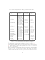
General purpose functions include:
cos(real or matrix)
sin(real or matrix)
tan(real or matrix)
abs(real or matrix)
exp(real or matrix)
srand(real or none)
rand()
min(real or matrix)
max(real or matrix)
Rows(matrix)
Cols(matrix)
Range(real,real)
Rank(matrix)
Cond(matrix)
Idn(real)
Trn(matrix)
EDec(matrix,real)
Clust(matrix,real)
Matrix(string)
Returns cos(); argument is in radians
Returns sin(); argument is in radians
Returns tan(); argument is in radians
Returns abs()
Returns natural exponent
Seeds random number generator
Returns a random integer between 0 and RAND MAX
Returns minimum entry in a matrix
Returns maximum entry in a matrix
Returns number of rows of a matrix
Returns number of columns of a matrix
Returns a row vector of integer numbers in the range
Returns rank of a matrix
Returns condition number of a matrix
Returns identity matrix of requested dimension
Returns transpose of a given matrix
Returns epsilon decomposition of a matrix
Returns clustered matrix
Returns a matrix read from file
Table 2.2: General purpose functions
Single argument math functions can take either a real number or a matrix.
In the case of a matrix input, function is applied to each matrix entry. The
four arithmetic operations have the usual meaning for real numbers. If one
of the operands is a matrix, the result depends on which of the operands is
the matrix. For addition/subtraction, if both operands are matrices, they
must be of the same dimensions and the result is the regular matrix addition/subtraction. If one of the operands is a matrix and the other one is a
13
real number, the addition/subtraction is done element wise. That is, it is
equivalent to addition/subtraction of two matrices where one of the matrices
has all the elements equal to the real number operand. Two real number
multiplication also has the usual meaning. If one of the operands is a real
number and the other one is a matrix, the result is the matrix multiplied by
a constant. Division has the usual interpretation for real numbers. If one of
the operands is a matrix and the other one is a real number, the operation is
done element wise. Since division is not commutative, either the real number or matrix elements can be the divisor. In the case of division, there can
also be a combination of two matrices of different dimensions. Depending
on the dimensions of the matrices, the result can be a solution of a single
system of linear equations, a number of linear equations, or a Least Square
Estimation (LSE). Matrices still must satisfy dimension requirements to be
able to perform these operations. The following example finds a solution of
a single system of linear equations AB = X; A is 3x3 and B is 3x1. This is
a determined system of equations.
ipsys> a = Matrix("3x3.mat");
ipsys> a(2,2) = -1;
ipsys> b = [1;1;1];
ipsys> printf("% 3.2f ",b/a);
[
-0.50 ;
0.00 ;
0.50
]
Next is an example of the solution of a system Ax = B where A is 3x3 and
B 3x2. This is still a determined system of equations.
ipsys> b = [1,2;1,3;1,4];
ipsys> printf("% 3.2f ",b/a);
[
-0.50 -0.50 ;
0.00 0.00 ;
0.50 0.83
]
14
Note that one of the solutions is the same as in the previous example. The
following is an example of an over determined system of equations. The solution is an LSE approximation.
a = [1, 2, 3;5, 4, 2; 7, 6, 4; 1, 2, 9];
ipsys> printf("Rank(a) = %g \n",Rank(a));
Rank(a) = 3
b = [1;1;1;1];
ipsys> printf("% 3.2f ",b/a);
[
-0.38 ;
0.65 ;
0.01
]
The result of this operation is the LSE approximation of the solution. Note
that the rank of a must be equal to the number of columns for this operation
to be possible. These results are typical for QR decomposition used to solve
systems of equations.
IPSYS also provides enough of the common programming constructs to be
able to write general purpose scripts. This includes condition tests, IFTHEN-ELSE conditional execution, WHILE, and FOR loops. With these
basic constructs, one should be able to perform other program flow controls.
Condition tests and logical operators implemented by IPSYS:
==
<
>
<=
>=
!=
&&
||
Equality test
Less than test
Greater than test
Less than or equal test
Greater than or equal test
Not equal test
Logical AND operator
Logical OR operator
Table 2.3: General purpose logical operators
Typical script with conditional tests:
15
ipsys> a = 0;
ipsys> if(a == 0){
b = 1.0;
} else {
b = 1/a;
}
ipsys> printf("%g\n",a);
0
IPSYS understands usual program flow control constructs. Loops are implemented using ”while” and ”‘for”’ constructs and the tests with ”if-then-else”
logical test. All the logical operators are discussed in section 2.2. The following is an example of typical use of test and looping in IPSYS:
ipsys> a = 0;
ipsys> b = 10;
ipsys> while(a < 5 && b > 0){
printf("a = %g\tb = %g\n",a,b);
a = a + 1;
b = b - 1;
}
a = 0
b = 10
a = 1
b = 9
a = 2
b = 8
a = 3
b = 7
a = 4
b = 6
Another way of looping through a series of calculations is by using for loops:
ipsys> for(i = 0; i < 5; i = i + 1){
printf("% 3.2g \n", i/5);
}
0
0.2
0.4
0.6
0.8
16
Flow control using continue, break, and goto statement are not implemented
since they are not necessary. Switch/case statement can be emulated with
with a more flexible if/else if construct:
ipsys> a = M_PI;
ipsys> if(a == M_PI_2)
printf("a is %g\n", M_PI_2);
else if(a == M_PI)
printf("a is %g\n", M_PI);
else
printf("a is not known\n");
a is 3.14159
Previous examples use printf function which is part of the I\O and is described in more detail in section 2.5.
17
2.3
Scripts and Functions
There are two mechanisms to automate and expand IPSYS capabilities. One
is by using include statement and the other one is by writing new scripting
and/or hard coded functions. New scripting functions can be either typed
from the command prompt or more commonly using the include statement.
Include statement simply includes a file that is automatically interpreted
as an IPSYS script. An include function can contain any statements that
might be used during an interactive IPSYS session. Such script files can be
used for function definition, repetitive data entry, and/or execution. As an
example, the following is the execution of an include statement:
ipsys>
c = [
0.93
-1.81
0.75
]
#include "Solve.ipsi";
1.32 ;
0.43 ;
0.44
where Solve.ipsi file contents is:
a = rand(3,3);
b = rand(3,2);
c = b/a;
printf("%5.2f ",c);
In this case, include is executed at the top level and the created variables are
global:
ipsys> lsVars();
stack level: 0
[a,
00A095F8]
[b,
00A096C8]
[c,
00A09888]
[a,
[b,
[c,
3x3 matrix]
3x2 matrix]
3x2 matrix]
IPSYS can use scripting and built in (hard coded) functions. From users’
perspective they are the same. Users can program both scripting and built in
(C++) functions. However, built in functions must be defined in IPSYS and
added to a lookup table in addition to compiling and linking the function.
18
These process is straight forward and explained in more details in the API
Manual. Scripting functions must be defined before used. Once defined without any errors, scripting functions are compiled into execution trees. Scripting functions can call built in functions and built in functions could easily
call scripting functions. Scripting function can be defined anywhere within
IPSYS session but the recommended method is by using include statement.
A function is defined similar to Matlab functions. The following example illustrates all of the function definition and calling features. LinSolve function
is defined in LinSolve.ipsi file as:
function [x,y] = LinSolve(a,b){
if(Rows(b) != Rows(a)){
printf("Incompatible dimensions\n");
return 0;
}
if(Rank(a) != Cols(a)){
printf("Rank deficient matrix a.\n");
return 0;
}
x = b/a;
}
and included in IPSYS workspace with:
#include "LinSolve.ipsi";
Now, LinSolve() function can be called in three different ways:
ipsys> #include "LinSolve.ipsi";
ipsys> a = rand(3,3);
ipsys> b = rand(3,2);
ipsys> [sol] = LinSolve(a,b);
ipsys> printf("% 5.2f ",sol);
sol = [
0.73 0.83 ;
1.94 0.48 ;
-1.80 -0.51
]
ipsys> printf("% 5.2f ",LinSolve(a,b));
[
19
0.73 0.83 ;
1.94 0.48 ;
-1.80 -0.51
]
ipsys> [sol,non] = LinSolve(a,b);
ipsys> printf("% 5.2f \n",non);
0.00
LinSolve() is defined to return two variables. Calling function can use both
variables, just one of them, or none. Return variables are assigned to variables in calling function’s memory space from left to right. In addition, if
only one variable is transfered, it must be the left most one and in that case
it does not need brackets as shown above. Also, if the function does not
return any variable, the default return value is zero. The following function
is perfectly acceptable and useless but it does produce a zero as the return
value:
ipsys> function [] = zero(){
};
ipsys> printf("%g\n",zero());
0
Each IPSYS function uses its own memory space and recursive calls can
be used as expected. The following example defines a recursive Fibonacci
function and shows its use:
ipsys> #include "fib.ipsi";
ipsys> f = fib(14);
ipsys> printf("%g\n", f);
233
ipsys>
where fib.ipsi file contains:
function [f] = fib(n){
if(n <= 1){
return 0;
} else if (n == 2){
return 1;
} else {
20
return (fib(n-2) + fib(n-1));
}
}
Application Programming Interface (API) and development of natively compiled functions is described in the API ”User’s Manual”. As far as function
user is concerned, there is no difference between calling a scripting function
or compiled function.
21
2.4
Power Systems Functions
IPSYS is based on the framework potentially providing interactive interface
for many different problems. To differentiate between different algorithm
types, power systems functions are prefixed with SSNet meaning steady
state network. Power systems functions can be grouped into two groups:
network input/output functions and network computational functions. Each
input/output function can be used for both input and/or output by allowing
for optional inputs. That is, if the function is to be used just to get an output
from the net, the optional arguments are omitted. If the same function is
to be used as an input to the net, the optional arguments contain the input
values.
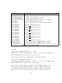
IPSYS network functions use a part of PTI23 data described in [4]. Currently, IPSYS uses bus, generator, switched shunts, and transformer adjustment data. However, both switched shunts and transformers are used as fixed
elements, that is their settings are not adjusted to control either bus voltage
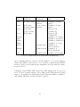
or branch real power flow. Power system input/output function description:
Function Name
SSNet
SSNetGen
SSNetGenST
SSNetLoad
SSNetVolt
SSNetShunt
SSNetPrint
SSNetPrintFlows
SSNetJac
SSNetG
SSNetB
SSNetCost
Function Description
Defines a network from a PTI file
and optional supply and demand files
Sets real power generation level
Sets generator status
Sets real and reactive load level
Sets voltage magnitude and angle of a bus
Sets shunt value on a given bus in a given system
Prints out PTI23 network data
Prints out power flows
Returns power flow jacobian
Returns G part of admittance matrix
Returns B part of admittance matrix
Returns productions cost
Table 2.4: Power system input/output functions
22
Power system output functions calling options and return values:
Function
Name
SSNet
SSNetGen
SSNetGenST
SSNetLoad
SSNetVolt
SSNetShunt
SSNetPrint
SSNetPrintFlows
SSNetJac
SSNetG
SSNetB
SSNetCost
Required
Arguments
1) net name
2) input file
3) supply file
4) demand file
1) net name
2) bus number
3) generator ID
1) net name
2) bus number
3) generator ID
1) net name
2) bus number
3) load ID
1) net name
2) bus number
1) net name
2) bus number
1) net name
1) net name
1) net name
1) net name
1) net name
1) net name
Optional
Arguments
Return
Values
(0??)
4) new P
5) new Q
1) old P
2) old Q
4) new ST
1) old ST
4) new P
5) new Q
1) old P
2) old Q
3)
4)
3)
4)
1)
2)
1)
2)
0
0
1)
1)
1)
1)
new
new
new
new
mag
ang
Gl
Bl
1) output file
old
old
old
old
Vmag
Vang
Gl
Bl
Jacobian
matrix G
matrix B
cost
Table 2.5: Power system input/output functions arguments
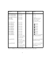
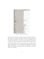
The implemented power system algorithms are described in Table 2.4.
Power system algorithm calling options and return values are shown in Table
2.6. SSNet function requires four arguments where some or all of the last
two can be empty strings.
Functions SSNetGen, SSNetGenST, SSNetLoad, SSNetVolt, and SSNetShunt
are used to get, set, or get old and set new values. For example, the following
command at the same time reads the old generator status value and sets the
23
Function Name
Function Description
SSNetNRPF
Newton-Raphson power flow
SSNetDCOPFFlexG
DC OPF with dispatchable generation
SSNetDCOPFFlexD
DC OPF with dispatchable demand
SSNetDCOPFFlexGD DC OPF with dispatchable generation and demand
SSNetDF
returns distribution factors matrix
SSNetDCFL
returns calculated DC flows using distribution matrix
SSNetMakeSens
calculates sensitivity matrices
g
SSNetDPgDT
Returns ∂P
and index vectors
∂θ
∂Pg
SSNetDPgDVg
Returns ∂Vg and index vectors
g
SSNetDPgDVl
Returns ∂P
and index vectors
∂Vl
∂Pl
SSNetDPlDT
Returns ∂θ and index vectors
∂Pl
SSNetDPlDVg
Returns ∂V
and index vectors
g
∂Pl
SSNetDPlDVl
Returns ∂Vl and index vectors
l
SSNetDQlDT
Returns ∂Q
and index vectors
∂θ
∂Ql
SSNetDQlDVg
Returns ∂Vg and index vectors
l
and index vectors
SSNetDQlDVl
Returns ∂Q
∂Vl
MatrixLMPSG
Returns LMPS while optimizing flexible generation
MatrixLMPSD
Returns LMPS while optimizing flexible demand
MatrixLMPSGD
Returns LMPS while optimizing flexible generation and demand
IPSYS Power system algorithms
new value:
ipsys> st4 = SSNetGenST("b6",4,"’1 ’",0);
ipsys> printf("previous generator on bus 4, id 1 status was %g\n",st4);
previous generator on bus 4, id 1 status was 1
while the next example just reads the status of the same generator:
ipsys> st4 = SSNetGenST("b6",4,"’1 ’");
ipsys> printf("current generator on bus 4, id 1 status is %g\n",st4);
current generator on bus 4, id 1 status is 0
The following group of functions calculate various sensitivity matrices. For
efficiency reasons, SSNetMakeSens() must be called to actually calculate all of
the sensitivities for the current operating conditions. Afterward, a sensitivity
matrix can be obtained using an appropriate function. All of these functions
24
return a sensitivity matrix and two index vectors defining the sensitivities.
For example:
ipsys> [dpgdvl, i, j] = SSNetDPgDVl("b6");
ipsys> printf("%g\t%g\n",i(1,1),j(1,1));
1
2
∂P
means that dpgdvl1,1 = ∂Vgl 1 . The only purpose of displaying the indexes is
2
for the users benefit. Indexes are used for original bus and should not be
used for indexing internal data structures. All of the sensitivity functions
take a Net variable as single argument and can be reliably used only after
calling SSNetMakeSens first.
The next group of calculates Locational Marginal Prices (LMP) while optimizing either the flexible supply,demand, or both. For example, SSNetLMPG(”all”,
[3, 1, 0.1]) finds nodal LMPs of network named ”all” when line 1 → 3 is congested using 0.1 increment and flexible supply. The first vector entry is
the node to which the price reference node is connected. The second argument is the price reference node, and the third argument is the transmission
constraint increment used to calculate Lagrangian multipliers. It is very important that the line is either congested or not for the both values of the
transmission limit. That is, a line should be either congested for both values of the transmission limit or for none. In the later case, all the LMP
values should be equal. Similarly, SSNetLMPSD(”all”,[3,1,0.1]); calculates
the LMPs assuming that the generation is fixed and the demand is flexible.
SSNetLMPSGD(”all”,) calculates the LMPs assuming that both generation
and demand are flexible. The same transmission congestion considerations
should be observed as in the previous two functions.
25
Function
Name
SSNetNRPF
SSNetDCOPFFlexG
SSNetDCOPFFlexD
SSNetDCOPFFlexGD
SSNetDF
SSNetDCFL
Required
Arguments
1) net name
1) net name
1) net name
1) net name
1) net name
1) net name
SSNetMakeSens
SSNetDPgDT
SSNetDPgDVg
SSNetDPgDVl
SSNetDPlDT
SSNetDPlDVg
SSNetDPlDVl
SSNetDQlDT
SSNetDQlDVg
SSNetDQlDVl
MatrixLMPSG
1) net name
1) net name
1) net name
1) net name
1) net name
1) net name
1) net name
1) net name
1) net name
1) net name
1) net name
2) row vector with
two adjacent nodes
and increment
1) net name
2) row vector with
two adjacent nodes
and increment
1) net name
2) row vector with
two adjacent nodes
and increment
MatrixLMPSD
MatrixLMPSGD
Optional
Arguments
2) [Pm,Qm,Iter]
Return
Values
1) [rank,Pm,Qm,Iter]
1) cost?
1) cost?
1) cost?
1) distribution factors
1) DC power flows
2) source buses
3) destination buses
1) 0?
g
1) ∂P
matrix
∂θ
∂Pg
1) ∂Vg matrix
g
1) ∂P
matrix
∂Vl
∂Pl
1) ∂θ matrix
∂Pl
1) ∂V
matrix
g
∂Pl
1) ∂Vl matrix
l
1) ∂Q
matrix
∂θ
∂Ql
1) ∂Vg matrix
l
1) ∂Q
matrix
∂Vl
1) bus indexes and LMPS
optimizing generation
1) bus indexes and LMPS
optimizing demand
1) bus indexes and LMPS
optimizing generation
and demand
Table 2.6: IPSYS power system algorithms calling options and return values
26
2.5
Input/Output and Miscellaneous
Functions
The API framework used for IPSYS can easily provide any functionality the
native C/C++ programming language provides. IPSYS implements screen
and file input/output, internal data structures listing, and some additional
miscellaneous functions.
As demonstrated throughout the previous examples, results can be displayed
using built in printf function. Similarly, fprintf function is used to write to
a file rather than to the screen. Both of these functions are similar to C
functions with the same names. Additionally, printf can print out a single
matrix using given format applied to each matrix entry. Format string is
just the regular C printf format string. Printing to a file is done using fprintf
which can also print a single matrix like printf. fprintf takes a file name as an
argument rather then a file descriptor. To be able to write to a file, file must
first be opened with fopen function which does not return file descriptor but
makes it globally visible using the file name. After writing to a file, the file
should be closed with fclose. Writing a matrix of random numbers between
0 and 1 in Matlab format to a file could be performed as:
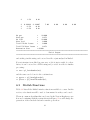
ipsys>
ipsys>
ipsys>
ipsys>
srand();
fopen("rand5x5.m","w");
fprintf("rand5x5.m","%7.3f", rand(5,5)/RAND_MAX);
fclose("rand5x5.m");
resulting in rand5x5.m file:
$ more rand5x5.m
[
0.847 0.033 0.614
0.344 0.085 0.877
0.203 0.757 0.817
0.707 0.197 0.395
0.240 0.449 0.085
]
0.009
0.334
0.044
0.833
0.933
0.236;
0.322;
0.927;
0.822;
0.971
Table 2.7 lists I/O functions and some miscellaneous functions. Functions
lsConsts, lsVars, lsFuncs, and lsMem list the available constants, variables
27
Function Required
Optional
Name
Arguments
Arguments
printf
1) format string 2) one or more
variables
fprintf
1) file name
3) one or more
2) format string variables
fopen
1) file name
2) mode string
fclose
1) file name
lsConsts
lsVars
lsFuncs
lsMem
clsVars
1) variable list
clsFuncs
1) functions list
sleep
1) miliseconds
Return
Value
1) number of chars
printed
1) number of chars
printed
1) success (1)
or failure (0)
1) success (1)
or failure (0)
1) number of constsnt
1) number of variables
1) number of functions
1) number of objects
1) number of
deleted variables
1) number of
deleted functions
1) miliseconds sleeping
Table 2.7: Input/Output and Miscellaneous Functions
used, scripting functions defined, and the number of objects in memory.
clsVars and clsFuncs can be used to clear variables or functions from IPSYS
memory; if they are used without any arguments, all of the variables or functions are cleared.
Sometimes, when IPSYS CLI controls the GUI display from a loop, it is
needed to slow down the display of the results on the GUI network. For this
purpose, sleep function is implemented which takes the number of milliseconds during which the execution should be paused.
28
Chapter 3
Matlab Interface
3.1
Introduction
Matlab Interactive Power Systems Simulator (MIPSYS) consists of algorithms described in 2.4. MIPSYS uses an older version of IPSYS algorithms
and its further development has been abandoned in favor of GUI interface
and its ability to export GIPSYS networks to Matlab environment. All of
the functionality provided by ipsys is also available through Matlab. Although there are other packages which have similar functionality, all of them
are rather difficult to use and integrate with the rest of Matlab. Matlab
interface to ipsys algorithms is designed with user friendliness in mind more
than efficiency. Both ipsys and Matlab interface are designed using object
oriented approach. While ipsys defines system as an object and and operates
on it, Matlab passes an object around from a function to a function. Due
to Matlab design, all the data is passed by value. This could result in lots
of data copying between function calls. Rather than using lots of static data
and be able to analyze a single system at the time, the performance penalty
is accepted for the sake of flexibility and user friendliness. The main interface
design decisions were to use array of structures to define a network in Matlab
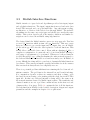
and to use pairs of Matlab/C++ mex functions to interface Matlab functions
with regular C++ functions. Since Matlab does not use namespaces, a convention is introduced where Matlab files in this package start with pl , C++
mex interface files with cpp and regular C++ functions not used in Matlab
are the same as before. Results using Matlab and ipsys should be exactly
the same since they are using the same code.
29
3.2
Matlab Interface Data
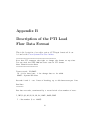
Matlab maps data read from a PTI23 file into a structure consisting of arrays
of network objects. That is, a net object has an array of buses, generators.
branches, etc. and each element of an array contains all of the data defined
in the PTI23 file for that particular element. For example, a six bus network
is defined in b6.p23 input file and its main structure in Matlab is given
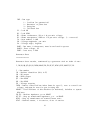
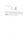
as: while, for example, array of buses is given as: The convention used for
Figure 3.1: Six Bus Data Structure
naming structure elements is that all the elements read in from the input file
are capitalized and any additional data is named with small letters. User
is free to change already existing elements or add new data. Description of
the capitalized elements can be found in Appendix B. Small letter variable
naming should be obvious and is listed in the following tables for network
elements actually used in this software: The mandatory data that the cpp
functions expect to be present in the network structure is the data read
from the PTI input file. There can also be additional information needed
for a particular algorithm. This additional data can include various cost
30
Figure 3.2: Bus 6 Data Structure
functions but user can freely keep any appropriate information within the
data structures. Currently, in addition to the bus record discussed above,
this software uses generator and branch records from the input PTI input
file and cost function files. Since this is work in development, there are
possibilities to define data not used by any algorithms yet. This will be
discussed in the function calling section. Table 3.1 lists elements not read
from the PTI input file but used in currently implemented algorithms. While
ipsys scripting language used special functions to manipulate network data,
Matlab allows direct access to all of the network structures. As with all
Matlab programming, vectorizing should be used as much as possible to
improve the performance.
31
swing
pvIndx
pqIndx
i
qmax
qmin
pg
qg
vaub
valb
vmub
vmlb
plt
plb
i
ireg
pgcost
i
j
Additional network data
Internal index of the swing bus
Internal indexes of the PV buses
Internal indexes of the PQ buses
Additional bus data
Internal numbering index
Maximum available VAR at the bus
Minimum available VAR at the bus
Real generation at the bus
Reactive generation at the bus
Upper voltage phase limit in degrees
Lower voltage phase limit in degrees
Upper voltage pu magnitude limit
Lower voltage pu magnitude limit
Upper load limit at the bus
Lower load limit at the bus
Additional generator data
Internal generator index
Internal index of a controlled bus
Coefficients of a real power cost polynomial
Additional branch data
Internal ”‘from bus”’ index
Internal ”‘to bus”’ index
Table 3.1: Additional Data
32
3.3
Matlab Interface Functions
Matlab interface to ipsys back end algorithms provides data input/output
and calculation functions. The input/output functions read and write data
from PTI23 network and cost polynomial files. Any subsequent reading,
modification, or deletion of the data is done through Matlab. The included
algorithms are the same ones as in ipsys and should give exactly the same
results. This section describes all of the interface function and similar descriptions can be viewed from Matlab using help function.
The design behind the Matlab interface uses a two step approach. User has
access to pl functions which in turn call cpp functions. This way, a user
has a two chances to process the input and/or output data, once in Matlab
pl file and in cpp file before the data is passed to back-end functions. This
should allow considerable data control. Even without changing pl files, a
complete reconfiguration of a network can be done from Matlab allowing a
wide range of experiments to be performed. Whenever a back-end function
is called through pl /cpp calling mechanism, the entire network is passed to
the back-end functions and treated as a brand new study case. In Matlab, it
is very difficult if not impossible to pass data to dynamically linked functions
by reference. This causes performance penalty but in this case it also ensures
that a network is always treated as completely new one.
There is a potential problem with functions returning the Jacobian and admittance matrix. The problems is the internal bus and branch indexing.
If a computation depends on these two matrices and their ordering, order
the buses in an increasing order starting with the slack bus in the PTI23
input file. In that case back-end internal ordering will be the same as in
the network structure formed by Matlab input routine. The sensitivity and
clustered matrices are not a problem contain indexes in the first row and
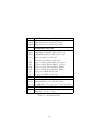
column as they do in ipsys. Table 3.2 contains the list of all the functions.
Use help function in Matlab for the detailed description of input and output
parameters and the examples in chapter 6 for a quick start.
33
Function Name
Data I/O Functions
pl pti23Net
pl printPGCostStr
pl printPLCostStr
pl printRawStr
pl NetFlows
Power Flow Algorithms
pl Admitt
pl DFFlows
pl DFactors
pl DPgDT
pl DPgDVg
pl DPgDVl
pl DPlDT
pl DPlDVg
pl DPlDVl
pl DQlDT
pl DQlDVg
pl DQlDVl
pl GSPF
pl Jacobian
pl NRPF
OPF Algorithms
pl DCOPFFlexD
pl DCOPFFlexG
pl DCOPFFlexGD
pl LMPSD
pl LMPSG
pl LMPSGD
Miscellaneous Functins
pl MClust
pl netUpdate
Input
Output
PTI 23 file name
Net structure
Net structure
Net structure
Net structure
Network structure
Pg cost functions string
Pl cost functions string
PTI 23 string
Net flows string
Net
Net
Net
Net
Net
Net
Net
Net
Net
Net
Net
Net
Net
Net
Net
Net admittance matrix
distribution factors flow
distribution factors
∂Pg
matrix
∂θ
∂Pg
matrix
∂Vg
∂Pg
matrix
∂Vl
∂Pl
matrix
∂θ
∂Pl
matrix
∂Vg
∂Pl
matrix
∂Vl
∂Ql
matrix
∂θ
∂Ql
matrix
∂Vg
∂Ql
matrix
∂Vl
Gauss-Seidel power flow
Net Jacobian
Newton-Raphson power flow
structure
structure
structure
Structure
structure
structure
structure
structure
structure
structure
structure
structure
structure
structure
structure
Net structure
Net structure
Net structure
Net structure,
node connected to ref.
node, ref. node, increment
same as pl LMPSD
same as pl LMPSD
DCOPF with flexible Pd
DCOPF with flexible Pg
DCOPF with flexible Pg and Pd
LMPS with flexible Pd
Real matrix
Net structure
Clustered matrix
Updates network variables
Table 3.2: Matlab Interface Functions
34
LMPS with flexible Pg
LMPS with flexible Pg and Pd
Chapter 4
GIPSYS Interface
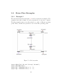
GIPSYS provides a GUI interface to all of the IPSYS functionality. However, GIPSYS GUI editor can be used to edit only a single network at the
time. GIPSYS consists of IPSYS CLI interface, script editor, and GUI power
systems network editor. IPSYS CLI interface is the same CLI interpreter described in chapter 2 with one difference. When entering multi line data or
commands, user must use SHIFT+RETURN or ENTER key to end each
line except the last one which is ended with the usual RETURN key. This
requirement is due to unexpected parser design restrictions but it will also
allow for much better error handling and reporting. The script (plain text)
and GUI editors are almost independent modules or libraries developed independently. The framework’s modular design makes addition of new modules
and interfaces quite easy. GIPSYS functionality is achieved through a number of menu entries and the CLI interface with the rest of IPSYS. GIPSYS
GUI design follows standard GUI interface as much as possible including file
opening, saving, closing, and exporting to other formats and/or graphics.
Edit menu includes adding new system elements such as buses, branches,
etc. but copying, cutting, and pasting is not implemented yet. Run menu
allows running the most common IPSYS algorithms. View menu provides
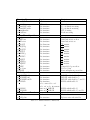
zooming in/out, snap-on, and choosing element label. Figure 4.1 shows all
three parts of the graphical user interface.
35
Figure 4.1: GIPSYS windows
4.1
Entering a New Network
At the start up, GIPSYS presents user with the CLI command window from
which text script and GUI editors can be opened. Text editor can be used
to open multiple text scripts at the same time while the GUI editor can be
used to edit a single network at the time. This network can also be accessed
from the CLI window using net name ”gnet”. The network editor is started
and closed from the main window with Tools→Start GUI and Tools→Close
GUI. To edit or start a new scrip use File→Open Script or File→New Script.
A new network can be entered with File→New, CTRL+N, or clicking on
New icon on the network editor tool bar. Once the user is presented with
the blank GIPSYS screen, network elements and connections can be entered
by first clicking on the element type on the tool bar or Edit menu and then
clicking at the desired location on the screen. Elements can be arranged
36
on the screen by dragging them around with the mouse. Two buses can be
connected with a branch by clicking on the branch edit menu entry and then
clicking on from and to bus in the network. A branch can be broken into
segments by first clicking on the branch to select it and then SHIFT+RIGHT
CLICK at the location of the desired joint. After the branch has one or more
joints, they can be dragged around with the mouse to arrange branch path
in a visually pleasing way. Elements can be attached to buses by choosing an
element and then clicking on the bus with which the element is associated.
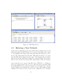
Typical start of a new network is shown in Figure 4.2. All system elements
Figure 4.2: New GIPSYS defined network
can have its typical measurements as a label and buses can have custom labels as well. This is done by using right mouse click on an element. Element
parameters dialog can be accessed by pressing right mouse button on an element and choosing Properties from the pop up menu or by using left double
click. Edit→Preferences defines the initial label option for each element.
GIPSYS GUI follows standard GUI design and users can expect similar features as in other applications with GUI interface. Network can be saved by
using File→Save As or clicking on the standard save icon on the tool bar. It
is users responsibility to provide one and only one slack bus for each network.
37
A network entered in the GUI editor window does not have to be saved
to be able to use it. Of course, the changes will not be available for the
next session unless they are saved on the hard drive. GUI editor can export
the edited network to PTI23 format files and two additional files containing
demand and generator cost functions. These files can be used with non-GUI
IPSYS interface described in chapter 2 or to use it with another package that
understands the PTI23 format. GUI editor can also export the network as
a picture for inclusion in publications and to Matpower format. The export
functions can be accessed with File→Export menu entry.
4.2
Running IPSYS Algorithms
Once a network is opened, it can be used either to run common algorithms
from the GUI editor interface or from the GUI CLI interface. The text interface provides much finer control over the execution of the algorithms then
the GUI interface can. Whatever is done through the GUI or command window is reflected in both environments. For example if the Newton-Raphson
power flow is run from the command window by issuing NRPF() command,
the results are reflected in the GUI window after the power flow is executed.
Similarly, if the Newton-Raphson power flow is executed from the GUI menu,
the IPSYS network object is modified accordingly. This setup allows for interesting and flexible visual demonstrations of how network might evolve.
For example, if loads are modified and power flow is run from within a loop,
voltage level changes can be observed visually on the GUI display using labels. Pause function can be used to slow down the execution to be able
to observe the output. To preserve data consistency during execution, GUI
window is disabled while CLI is executing a command and similarly, CLI
window is disabled while GUI command is executing.
Since the entire internal representation of the network (GUI and CLI) is
updated with every change, network can be continuously and programmatically changed and manipulated through functions and scripts. The disadvantage of this design approach is that the network can be, and is frequently
during editing, in an invalid state, for example slack bus is missing, existence of isolated buses, etc. This is not a problem as long as an operation
is not performed that requires a well defined network. Various commercial
packages address this by separating editing and running with Edit and Run
38
mode. This is a good solution but limits what can be done using scripts.
Accidentally, these packages also have limited scripting capabilities.
39
Chapter 5
IPSYS Examples
This chapter shows some examples how some of the major IPSYS features
introduced in the previous chapter can be used. The first section illustrates
linear algebra capabilities such as matrix input, matrix manipulation, general purpose functions, and linear algebra algorithms available. The second
section demonstrates input/output facilities. The rest of the examples deal
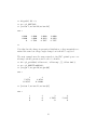
with power systems manipulation and analysis. Implementation details and
the theory behind this algorithms can be found in the appendices. All of the
examples will use the following data files:
1. b3.raw is three bus PTI raw data file
2. b3.sup generator cost curves
3. b3.dmd demand cost curves data
4. b6.raw six bus PTI raw data file
5. b6.sup generator cost curves
6. b6.dmd demand cost curves
and should be included with this manual. The examples emhasize power
systems features more than how to use IPSYS interface, which should be
intuitive enough.
All of the algorithms are implemented using dense matrix methods from
IMSL library [3] version 6.0 academic edition, and Template Numerical Toolkit
(TNT) [5].
40
5.1
Linear Algebra
This section demonstrates general numerical and linear algebra ipsys features.
5.1.1
Checking Rank and Condition Number
This example shows how a matrix can be constructed element by element
and checked for the condition number and rank:
ipsys> h = Matrix(5,5,0);
ipsys> for(i = 1; i <= Rows(h); i = i+1){
for(j = 1; j <= Cols(h); j = j+1){
h(i,j) = 1/(i+j-1);
}
}
ipsys> printf("\n%g\n", Cond(h));
476607
ipsys> printf("\n%g\n", Rank(h));
5
5.1.2
Sensitivity Matrix Extraction
In the power systems operations it is important to be able to extract parts of
a matrix. For example, some of the sensitivity matrices that ipsys calculates
l
can be extracted from the Jacobian matrix. Here is an example of how ∂Q
∂θ
can be extracted from the Jacobian matrix:
ipsys> SSNet("b6","b6.raw","","");
ipsys> SSNetNRPF("b6", [0.000001,0.000001,50]);
ipsys> jac = SSNetJac("b6");
ipsys> dqldt = jac(Range(6,Rows(jac)),Range(1,5));
ipsys> SSNetMakeSens("b6");
ipsys> printf("%g ", SSNetDQlDT("b6"));
[
-6.0712 0.0268085 0 0 0.877069 ;
-0.0268085 -1.2 0 0.190515 0 ;
0 -0.190515 0.725736 -1.2 0.664779
41
]
ipsys> printf("%g ", dqldt);
dqldt = [
-6.0712 0.0268057 0 0 0.877071 ;
-0.0268057 -1.20001 0 0.190516 0 ;
0 -0.190516 0.725739 -1.20001 0.664782
]
According to the above example, SSNetDQlDT function is not really necessary but is provided for user’s convenience.
5.1.3
Matrix Decomposition and Clustering
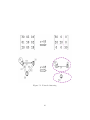
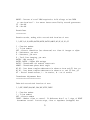
Epsilon decomposition and clustering can be used replacing one large network
with a few smaller, loosely coupled networks [8]. IPSYS provides two, almost
equivalent function for this task. The first one, Clust(mat,eps) implements a
general network clustering algorithm described in [6] which takes a weighted
undirectional graph and a weight threshold below which connections are ignored. This function returns a clustered matrix resulting from ignoring small,
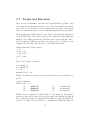
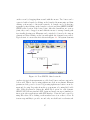
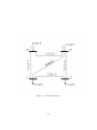
below eps threshold, connections and two vectors of the original matrix coordinates. Figure 5.1 illustrates this approach to system reduction. The second
function, EDec(mat,eps), calculates the same decomposition but it returns a
matrix with number of rows equal to the number of clusters where each row
contains row indexes of the original matrix. These two functions give equivalent results except possibly different permutations within a cluster. EDec()
combined with SSNetJac(), and SSNetNRPF() was used in [8] to decompose
and analyze the standard IEEE test network RTS-1996.
42
Figure 5.1: Network clustering
43
5.2
5.2.1
Power Flow Examples
Example 1
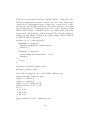
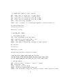
The six bus network shown in figure 5.2 is used for the next 4 examples. The
examples start with a simple one and progressively become more complex.
The first example is just a power flow runs for a couple of different operating
points. First, calculate the generation cost for the first operating point:
Figure 5.2: Six bus system
ipsys>
ipsys>
ipsys>
ipsys>
SSNet("b6","b6.raw","b6.sup","b6.dmd");
SSNetNRPF("b6");
Pg4 = SSNetGen("b6",4,"’1 ’");
Pg6 = SSNetGen("b6",6,"’1 ’");
44
ipsys> Pg1 = SSNetGen("b6",1,"’1 ’");
ipsys> GenCost = SSNetCost("b6");
ipsys> printf("Pg1 = %7.2f\tPg4 = %7.2f\tPg6 = %7.2f\tGenCost = %7.2f\n",Pg1,Pg4
,Pg6,GenCost);
Pg1 = 272.20
Pg4 = 186.36
Pg6 = 148.03
GenCost = 580.91
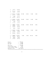
Now, change the generator output of the generator on bus four and calculate
the generation cost again:
ipsys> SSNetGen("b6",4,"’1 ’",150);
ipsys> SSNetNRPF("b6");
ipsys> Pg1 = SSNetGen("b6",1,"’1 ’");
ipsys> Pg4 = SSNetGen("b6",4,"’1 ’");
ipsys> Pg6 = SSNetGen("b6",6,"’1 ’");
ipsys> GenCost = SSNetCost("b6");
ipsys> printf("Pg1 = %7.2f\tPg4 = %7.2f\tPg6 = %7.2f\tGenCost = %7.2f\n",Pg1,Pg4
,Pg6,GenCost);
Pg1 = 308.91
Pg4 = 150.00
Pg6 = 148.03
GenCost = 585.23
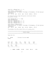
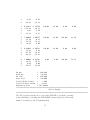
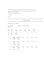
Newton-Raphson Power Flow solution for the second operating point is:
===============================================================================
Solution Output
===============================================================================
Input data file:
0
100.00
GIPSYS
From
Bus
-----To
Bus
------
Volt.
Mag.
--------Mw
Flow
---------
1
1.00000
/ Tue Mar 27 16:21:28 2007
Volt.
Mw
Mvar
Mw
Mvar
Angle
Load
Load
Gen.
Gen.
--------- --------- --------- --------- --------Mvar
Flow
--------0.00000
120.00
45
24.00
308.91
0.00
2
3
4
39.73
113.13
36.05
-19.09
31.09
0.33
2
1
3
6
0.98112
-37.78
-5.00
-82.22
-3.43660
21.03
-9.71
-35.32
125.00
24.00
0.00
0.00
3
1
2
5
0.98608
-113.13
5.00
-11.87
-3.28854
-24.21
9.78
-9.57
120.00
24.00
0.00
0.00
4
1
5
6
1.00000
-36.05
65.97
0.08
-1.03295
0.33
19.20
0.00
120.00
24.00
150.00
0.00
5
3
4
6
0.99095
11.87
-65.97
-65.89
-2.94059
9.69
-16.84
-16.84
120.00
24.00
0.00
0.00
6
2
4
5
1.00000
82.22
-0.08
65.89
-1.03526
39.47
0.00
19.20
0.00
0.00
148.03
0.00
Mw gen
=
606.942
Mvar gen
=
0.000
Mw load
=
605.000
Mvar load
=
120.000
Total I2R Mw losses
=
1.942
Total I2X Mvar losses =
18.532
Generation Cost
= 585.227777
===============================================================================
46
End of Output
===============================================================================
47
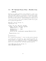
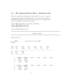
5.3
DC Optimal Power Flow - Flexible Generation
In the previous example, generation cost was calculated for a couple of operating points. In this example, a cost dependency on the generators on buses
four and six will be shown. The same network 5.2 is used for this example.
Bus number one is the slack bus and its generation cost is accounted for but
it is not shown in the graph due to dimensional limitations. Both generators
on buses four and six are varied between 50MW and 300MV. The script file
used to generate the graph data is:
SSNet("b6","b6.raw","b6.sup","");
fopen("b6.dat","w");
for(pg4 = 50; pg4 <= 300; pg4 = pg4+10){
for(pg6 = 50; pg6 <= 300; pg6 = pg6+10){
SSNetGen("b6",4,"’1 ’",pg4);
SSNetGen("b6",6,"’1 ’",pg6);
SSNetNRPF("b6");
fprintf("b6.dat","%g\t%g\t%g\n",pg4,pg6,SSNetCost("b6"));
}
fprintf("b6.dat","\n");
}
fclose("b6.dat");
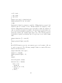
The cost graph is shown in figure 5.3. A user can easily generate such graphs
to get a feel for how cost depends on a couple of generators and maybe estimate the minimal cost operating point. If there is a large number of generators that can be used to minimize the generation cost, IPSYS DCOPFFlexG
function can be used instead and for the same network it is given by:
ipsys> SSNet("b6","b6.raw","b6.sup","");
ipsys> SSNetDCOPFFlexG("b6");
48
Figure 5.3: Production cost profile
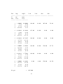
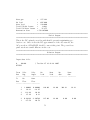
The minimal cost point found using DCOPFFlexG() function:
===============================================================================
Solution Output
===============================================================================
Input data file:
0
100.00
GIPSYS
From
Volt.
/ Tue Mar 27 16:21:28 2007
Volt.
Mw
Mvar
49
Mw
Mvar
Bus
-----To
Bus
------
Mag.
--------Mw
Flow
---------
1
2
3
4
1.00000
2.14
17.74
-134.80
0.00000
8.74
21.73
4.55
120.00
24.00
305.00
59.02
2
1
3
6
0.98914
-2.06
30.62
-153.56
0.38268
-8.66
0.18
-15.51
125.00
24.00
0.00
0.00
3
1
2
5
0.98918
-17.74
-30.62
-71.64
-0.51387
-21.34
0.30
-2.96
120.00
24.00
0.00
0.00
4
1
5
6
1.00000
134.80
79.06
-33.86
3.86468
4.55
18.91
0.29
120.00
24.00
150.00
47.74
5
3
4
6
0.99133
71.64
-79.06
-112.58
1.57948
5.59
-15.60
-13.98
120.00
24.00
0.00
0.00
6
2
4
5
1.00000
153.56
33.86
112.58
4.83466
27.68
0.29
20.53
0.00
0.00
150.00
48.50
Mw gen
Angle
Load
Load
Gen.
Gen.
--------- --------- --------- --------- --------Mvar
Flow
---------
=
605.000
50
Mvar gen
=
155.262
Mw load
=
605.000
Mvar load
=
120.000
Total I2R Mw losses
=
0.081
Total I2X Mvar losses =
35.275
Generation Cost
= 583.025000
===============================================================================
End of Output
===============================================================================
This is the DC optimal power flow with flexible generation minimizing production cost. Since it uses the DC approximation of the AC network, the
AC power flow, SSNetNRPF, should be run at this point. The power flows
print out shows a small difference in the cost:
===============================================================================
Solution Output
===============================================================================
Input data file:
0
100.00
GIPSYS
/ Tue Mar 27 16:21:28 2007
From
Bus
-----To
Bus
------
Volt.
Mag.
--------Mw
Flow
---------
Volt.
Mw
Mvar
Mw
Mvar
Angle
Load
Load
Gen.
Gen.
--------- --------- --------- --------- --------Mvar
Flow
---------
1
2
3
4
1.00000
39.41
112.40
35.10
0.00000
-18.87
30.98
0.31
120.00
24.00
306.91
36.41
2
1
0.98120
-37.50
-3.40520
20.78
125.00
24.00
0.00
0.00
51
3
6
-4.66
-82.84
-9.64
-35.14
3
1
2
5
0.98611
-112.40
4.66
-12.26
-3.26720
-24.18
9.70
-9.51
120.00
24.00
0.00
0.00
4
1
5
6
1.00000
-35.10
65.79
-0.69
-1.00557
0.31
19.18
0.00
120.00
24.00
150.00
43.49
5
3
4
6
0.99096
12.26
-65.79
-66.47
-2.90781
9.64
-16.83
-16.81
120.00
24.00
0.00
0.00
6
2
4
5
1.00000
82.84
0.69
66.47
-0.98583
39.35
0.00
19.20
0.00
0.00
150.00
58.55
Mw gen
=
606.908
Mvar gen
=
138.444
Mw load
=
605.000
Mvar load
=
120.000
Total I2R Mw losses
=
1.909
Total I2X Mvar losses =
18.452
Generation Cost
= 585.146048
===============================================================================
End of Output
===============================================================================
The AC power flow should also be used after DCOPF to check the operating
point feasibility by checking the SSNetNRPF return values (Jacobian rank,
number of iterations, and P/Q mismatches).
52
5.4
DC Optimal Power Flow - Flexible Load
If there is demand control implemented, there should be a way to account for
the demand flexibility. This Example shows such a hypothetical situation.
DCOPFFlexD() example uses the same b6.raw as the above example. Ipsys
script is very similar to the previous example:
ipsys> SSNet("b6","b6.raw","b6.sup","b6.dmd");
ipsys> SSNetDCOPFFlexD("b6");
ipsys> SSNetPrintFlows("b6");
and the DCOPFFlexD() result is:
===============================================================================
Solution Output
===============================================================================
Input data file:
0
100.00
GIPSYS
/ Tue Mar 27 16:21:28 2007
From
Bus
-----To
Bus
------
Volt.
Mag.
--------Mw
Flow
---------
Volt.
Mw
Mvar
Mw
Mvar
Angle
Load
Load
Gen.
Gen.
--------- --------- --------- --------- --------Mvar
Flow
---------
1
2
3
4
1.00000
10.25
0.00
0.00
0.00000
10.25
33.40
0.00
64.39
24.00
0.00
0.00
2
1
3
6
0.97950
-10.04
0.00
0.00
0.00000
-10.04
-7.44
-40.16
10.00
24.00
0.00
0.00
53
3
1
2
5
0.98330
0.00
0.00
0.00
0.00000
-32.84
7.47
-2.95
50.00
24.00
0.00
0.00
4
1
5
6
1.00000
0.00
0.00
0.00
0.00000
0.00
30.40
0.00
200.00
24.00
186.36
24.69
5
3
4
6
0.98480
0.00
0.00
0.00
0.00000
2.95
-29.94
-29.94
10.00
24.00
0.00
0.00
6
2
4
5
1.00000
0.00
0.00
0.00
0.00000
41.00
0.00
30.40
0.00
0.00
148.03
76.96
Mw gen
=
334.394
Mvar gen
=
101.646
Mw load
=
334.394
Mvar load
=
120.000
Total I2R Mw losses
=
0.210
Total I2X Mvar losses =
2.566
Generation Cost
= 370.716924
===============================================================================
End of Output
===============================================================================
54
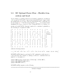
5.5
DC Optimal Power Flow - Flexible Generation and Load
As an example of optimal generation and demand calculations, calculations
of [1] on pages 157-158 will be done by hand, using IPSYS and compared with
the results in the above paper. The four bus network under consideration is
shown in figure 6.1. Power flow shows that flow PG1→L1 exceeds the branch
max
maximum flow PG1→L1
given as 3.7pu. Using this fact as a binding constraint and setting up the Lagrange equation for constrained optimization,
the following set of equations results:



2
0
0
0
0
0
0
−1 0
0
0
0
−1
 0

 −0.5
4
0
0
0
0
0
0
−1
0
0
0



 0

 94.1667
0
20
0
0
0
0
0
0
−1
0
0



 0

 158.1667
0
0
24
0
0
0
0
0
0
−1
0



 0

 0
0
0
0
0
0
0
−1 3
1
1
0 


 0


0
0
0
0
0
0
−1
−1
−3
1
−1

z =  0
 0
 0
0
0
0
0
0
0
0
−1 1
−2 0 



 −1 0

 0
0
0
−1
−1
0
0
0
0
0
0




 0
 0
−1
0
0
3
−1
−1
0
0
0
0
0



 0

 0
0
−1 0
1
−3 1
0
0
0
0
0 


 0
 0
0
0
−1 1
1
−2 0
0
0
0
0 
0
0
0
0
0
−1 0
0
0
0
0
0
3.7




















with the following solution:
0
z = 5.45 4.07 3.70 5.82 −1.75 −3.70 −5.63 11.91 16.79 −20.04 −18.42 13.02
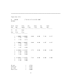
DCOPFFlexGD() function performs the DC optimization with respect to
both generation and demand accounting for the flow constraint from bus
number 1 to bus number 3:
ipsys> SSNet("all","allen.raw","allen.sup","allen.dmd");
ipsys> SSNetDCOPFFlexGD("all");
ipsys> SSNetNRPF("all");
DCOPFFlexGD() output is as the following:
===============================================================================
Solution Output
55
===============================================================================
Input data file:
0
100.00
GIPSYS
/ Tue Oct 25 16:18:59 2005
From
Bus
-----To
Bus
------
Volt.
Mag.
--------Mw
Flow
---------
1
2
3
1.00000
1.76
3.70
0.00000
0.02
0.13
0.00
0.00
5.46
0.15
2
1
4
3
1.00000
-1.76
3.88
1.95
-1.00607
0.02
0.15
0.08
0.00
0.00
4.07
0.25
3
1
2
4
0.99939
-3.70
-1.95
1.94
-2.12135
0.01
-0.04
0.04
3.71
0.00
0.00
0.00
4
2
3
0.99922
-3.88
-1.94
-3.23376
-0.00
0.00
5.82
0.00
0.00
0.00
Mw gen
Mvar gen
Mw load
Mvar load
Volt.
Mw
Mvar
Mw
Mvar
Angle
Load
Load
Gen.
Gen.
--------- --------- --------- --------- --------Mvar
Flow
---------
=
=
=
=
9.529
0.394
9.529
0.000
56
Total I2R Mw losses
=
0.000
Total I2X Mvar losses =
0.394
Generation Cost
= 71.936386
===============================================================================
End of Output
===============================================================================
IPSYS calculations agree closely with the hand calculations above and the
results reported in [1]:
G1 (M W )
G2 (M W )
L1 (M W )
L2 (M W )
G1 ($)
G2 ($)
L1 ($)
L2 ($)
F12 (M W )
F12 ($)
hand calculation
5.4552
4.0734
3.7059
5.8227
11.9104
16.7937
20.0492
18.4214
3.70000
13.0222
paper reported
5.4553
4.0734
3.7059
5.8227
11.9106
16.7936
20.0487
18.4219
3.70000
IPSYS
5.45517
4.07342
3.70587
5.82273
11.91
16.79
20.05
18.42
3.70
13.02
Table 5.1: Optimal welfare calculations
Although the numbers are almost exactly the same, [1] discusses the market
setup as a multilateral transaction while the above is the poolco formulation.
Nevertheless, the both formulations find the same optimal point.
57
Chapter 6
Matlab Examples
In this chapter, a few examples are used to demonstrate the main Matlab
interface features. For the demonstration purposes, a four bus network 6.1,
with associated real power cost functions, and real power demand functions
is used.
6.1
Matlab Input Output
Matlab and ipsys use the same input file formats. There are currently three
different input files that can be used by Matlab to define a power systems network. The only mandatory input file is the network definition file in PTI23
format. The other two files provide the real power generation cost and the
load demand. The internal functions do limited checking of compatibility
of these three files and user should pay attention that the real power limits
in PTI23 file match the real power limits in defined by the cost functions.
Also, PTI23 allows only a single load per bus. To allow for a possibility of
multiple loads per bus, the demand file should use the default ’1 ’ as the load
ID until a multi load options is implemented. Even in the currently used
format, there can be multiple generators on a single bus and they should be
named as described by PTI23 format in Appendix B.
pl pti23Net is the Matlab function used to read both network description
and cost functions. It takes up to five arguments of which only the first one
is required and returns the net structure. The first argument is the name of
the PTI23 input file, the second argument is the Pg cost functions file, the
58
third argument is the Qg costs file, the fourth is Pl costs and the fifth is the
Ql demand curves file. Of this five parameters, only the first one is required
and Qg and Ql are to be used in the future. If an argument must be entered
but unused, use and empty matrix []. For example, the following will read in
the data for the system in the Figure 6.1:
>> b4 = pl_pti23Net(’allen.raw’,’allen.sup’,[],’allen.dmd’)
b4 =
Title1:
Title2:
Title3:
IC:
SBASE:
bus:
gen:
branch:
swing:
pvIndx:
pqIndx:
’0
100.00
’GIPSYS’
’’
0
100
[1x4 struct]
[1x2 struct]
[1x5 struct]
1
2
[2x1 double]
/ Tue Oct 25 16:18:59 2005’
Once the system data is read in, any of the algorithms listed in table 3.2 can
be applied to the system. As explained before, Matlab passes data by value,
so the arguments remain unaffected and the results can be captured through
the return value only. For example the following runs Newton-Raphson power
flow on the above network and prints out the voltages:
>> nt = pl_NRPF(b4);
>> [nt.bus.I;nt.bus.VM;nt.bus.VA]
ans =
1.0000
1.0000
0
2.0000
1.0000
-1.4332
3.0000
0.9993
-2.5803
4.0000
0.9993
-3.4406
Network structure data can be at any point used to extract and or change
data using usual Matlab methods. Matlab provides a large number of functions to extract whatever information is needed and present it in whatever
59
Figure 6.1: Four Bus System
60
format is desired with great flexibility. If it is desired to get the same line
flows output as with ipsys interface, the following function would return a
Matlab string with the flows:
>> flows = pl_NetFlows(nt);
>> flows
flows =
===============================================================================
Solution Output
===============================================================================
Input data file: unknown
0
100.00
GIPSYS
/ Tue Oct 25 16:18:59 2005
From
Bus
-----To
Bus
------
Volt.
Mag.
--------Mw
Flow
---------
Volt.
Mw
Mvar
Mw
Mvar
Angle
Load
Load
Gen.
Gen.
--------- --------- --------- --------- --------Mvar
Flow
---------
1
2
3
1.00000
2.50
4.50
0.00000
0.03
0.17
0.00
0.00
7.00
0.20
2
1
4
3
1.00000
-2.50
3.50
2.00
-1.43318
0.03
0.13
0.09
0.00
0.00
3.00
0.25
3
1
2
0.99932
-4.50
-2.00
-2.58029
0.03
-0.05
5.00
0.00
0.00
0.00
61
4
1.50
0.01
4
2
3
0.99930
-3.50
-1.50
-3.44065
-0.01
0.01
5.00
0.00
0.00
0.00
Mw gen
=
10.000
Mvar gen
=
0.451
Mw load
=
10.000
Mvar load
=
0.000
Total I2R Mw losses
=
0.000
Total I2X Mvar losses =
0.451
Generation Cost
= 0.000
===============================================================================
End of Output
===============================================================================
and at this point the string can be stored in a file or just analyzed in Matlab.
If a net structure is modified in some way or if it is just a result of a calculation, it can be stored in a PTI23 string and/or saved in a file for further
processing:
>> raw = pl_PrintRawStr(nt);
and the same can be done for the cost functions:
>> pgcost = pl_PrintPgCost(nt);
>> plcost = pl_PrintPLCostStr(nt);
6.2
Matlab Functions
Table 3.2 lists all the Matlab interface functions available to a user. In this
section, a few functions will be used to demonstrate how they can be used.
The most common algorithm that can be used is the Newton-Raphson power
flow and continuing with the system shown in Figure 6.1 we will change the
generation of the non-slack bus and rerun the power flow:
62
>> b4.gen(2).PG = 2;
>> nt = pl_NRPF(b4);
>> [nt.bus.I;nt.bus.VM;nt.bus.VA]
ans =
1.0000
1.0000
0
2.0000
1.0000
-1.7916
3.0000
0.9993
-2.7955
4.0000
0.9993
-3.7275
>>
Note that due the change in generation distribution, voltage magnitudes remained the same but voltage angles changed as it should be expected.
The next example uses the same network to find DC optimal power considering both the generators and loads to be flexible:
>> b4 = pl_pti23Net(’allen.raw’,’allen.sup’,[],’allen.dmd’);
>> nt = pl_DCOPFFlexGD(b4);
>> [nt.gen.I;nt.gen.PG;nt.gen.QG]
ans =
1
5.4552
0.14527
2
4.0734
0.24908
>> [nt.bus.I;nt.bus.PL;nt.bus.QL]
ans =
1
0
0
2
0
0
3
3.7059
0
63
4
5.8227
0
Chapter 7
Notes, Bugs, TODO list
IPSYS and implementation of all the underlying algorithms are results of
recent development, not rigorously tested and work in progress. Further
development can be done in the area of fixing bugs and providing new functionality. User feedback is crucial for both of these areas. This program is
being actively developed.
Detecting, reporting, and dealing with errors is one of the most difficult
aspects of interpreter and compiler design. Detecting errors can cause the
interpreter to just abort the entire program, try to process as much of the
input as possible and continue working and/or report the error back to the
user. Helpful error reporting includes a fair amount of guessing of what is
wrong with the input. IPSYS is a simple interface to a number of complex
algorithms and is more focused on algorithm implementation and less on error handling. As the result, error reporting and sometimes recovery is quite
limited. Following is the list of known bugs that are being worked on:
1. Running loops from the command line will slow GUI display update
if the network window is moved or overlapped during loop execution.
This seems to be operating system (Windows) related.
2. If a name is not associated with a function or data, the interpreter
reports that there is no matrix with such a name. This is a consequence
of using the same parenthesis type for indexing matrices and calling
functions.
3. A function must be defined before called. This will be changed by
64
introducing function declaration since two functions cannot call each
other unless they are the same function, that is unless if it is a recursive
call.
4. A defined function cannot be redefined within the same session.
5. Multi line commands in GUI must be ended with ENTER or SHIFT+RETURN
except the last one which is ended with the usual RETURN key.
The error reporting needs to be improved. This is just a time consuming
task. There are surely many more bugs. Any bug reports will be greatly
appreciated and addressed. There are also a few unfinished things:
1. SSNetPrint function not completed.
2. Transformer editing and use is incomplete in GUI.
3. Introduce function declaration; the lack of it affects both GUI and CLI
interface.
4. History saving menu is not functional yet.
65
Bibliography
[1] Eric Allen, Marija Ilic, and Ziad Younes. Providing for transmission in
times of scarcity: an iso cannot do it all. Electrical Power and Energy
Systems, 21:147–163, 1999. 55, 57
[2] IEEE Tutorial Course. Optimal Power Flow: Solution Techniques, Requirements and Challenges. 1996. 77
[3] Visual Numerics. IMSL C/Math/Library User’s Manual. Visual Numerics,Inc., 2000. 40
[4] University of Washington Department of Electrical Engineering.
http://www.ee.washington.edu/research/pstca/formats/pti.txt. 3, 22
[5] Roldan Pozo. Template numerical toolkit, an interface for scientific computing in c++. http://math.nist.gov/tnt/index.html. 40
[6] D. D. Shiljak. Decentralized Control of Complex Systems. Academic
Press, 1991. 42
[7] Allen J. Wood and Bruce F. Wollenberg. Power Generation Operation
and Control. John Wiley & Sons, Inc., 1996. 73, 79
[8] Le Xie, Jovan Ilić, and Marija Ilić. Towards grid modernization through
enhanced communications and computing: Novel performance index and
information structure for monitoring voltage problems. Carbondale, Il,
2006. North American Power Symposium. 42
66
Appendix A
Installation
GIPSYS and MIPSYS probably require Windows 2000 or Windows XP while
IPSYS could run on a less powerful computer and operating system. Installation of IPSYS and accompanying interfaces is almost automatic in Windows
environment. An auto-installation executable is provided which copies all
necessary files to a user chosen directory. All the necessary environment
variables needed to run IPSYS and GIPSYS are entered into Windows registry. However, if MIPSYS is to be used, user must add in Matlab path to
package’s pl *.m and cpp *.dll files. This is done using addpath() Matlab
command. To remember the new path between different Matlab sessions,
run savepath() command after the last addpath(). At this point, all three
interfaces should be functional.
67
Appendix B
Description of the PTI Load
Flow Data Format
This is the description of an earlier version of PTI input format and it can
be found at the Power Systems Test Case Archive.
============================================
Note that PTI reserves the right to change the format at any time.
For use with the IEEE 300 bus test case in PTI format.
Case Identification Data
========================
First record: IC,SBASE
IC - 0 for base case, 1 for change data to be added
SBASE - System MVA base
Records 2 and 3 - two lines of heading, up to 60 characters per line
Bus Data
========
Bus data records, terminated by a record with a bus number of zero.
I,IDE,PL,QL,GL,BL,IA,VM,VA,’NAME’,BASKL,ZONE
I - Bus number (1 to 29997)
68
IDE - Bus type
1 - Load bus (no generation)
2 - Generator or plant bus
3 - Swing bus
4 - Islolated bus
PL - Load MW
QL - Load MVAR
GL - Shunt conductance, MW at 1.0 per unit voltage
BL - Shunt susceptance, MVAR at 1.0 per unit voltage. (- = reactor)
IA - Area number, 1-100
VM - Voltage magnitude, per unit
VA - Voltage angle, degrees
NAME - Bus name, 8 characters, must be enclosed in quotes
BASKV - Base voltage, KV
ZONE - Loss zone, 1-999
Generator Data
==============
Generator data records, terminated by a generator with an index of zero.
I,ID,PG,QG,QT,QB,VS,IREG,MBASE,ZR,ZX,RT,XT,GTAP,STAT,RMPCT,PT,PB
I - Bus number
ID - Machine identifier (0-9, A-Z)
PG - MW output
QG - MVAR output
QT - Max MVAR
QB - Min MVAR
VS - Voltage setpoint
IREG - Remote controlled bus index (must be type 1), zero to control own
voltage, and must be zero for gen at swing bus
MBASE - Total MVA base of this machine (or machines), defaults to system
MVA base.
ZR,ZX - Machine impedance, pu on MBASE
RT,XT - Step up transformer impedance, p.u. on MBASE
GTAP - Step up transformer off nominal turns ratio
STAT - Machine status, 1 in service, 0 out of service
69
RMPCT - Percent of total VARS required to hold voltage at bus IREG
to come from bus I - for remote buses controlled by several generators
PT - Max MW
PB - Min MW
Branch Data
===========
Branch records, ending with a record with from bus of zero
I,J,CKT,R,X,B,RATEA,RATEB,RATEC,RATIO,ANGLE,GI,BI,GJ,BJ,ST
I - From bus number
J - To bus number
CKT - Circuit identifier (two character) not clear if integer or alpha
R - Resistance, per unit
X - Reactance, per unit
B - Total line charging, per unit
RATEA - MVA rating A
RATEB, RATEC - Higher MVA ratings
RATIO - Transformer off nominal turns ratio
ANGLE - Transformer phase shift angle
GI,BI - Line shunt complex admittance for shunt at from end (I) bus, pu.
GJ,BJ - Line shunt complex admittance for shunt at to end (J) bus, pu.
ST - Initial branch status, 1 - in service, 0 - out of service
Transformer Adjustment Data
===========================
Ends with record with from bus of zero
I,J,CKT,ICONT,RMA,RMI,VMA,VMI,STEP,TABLE
I - From bus number
J - To bus number
CKT - Circuit number
ICONT - Number of bus to control. If different from I or J, sign of ICONT
determines control. Positive sign, close to impedance (untapped) bus
70
of transformer. Negative sign, opposite.
RMA - Upper limit of turns ratio or phase shift
RMI - Lower limit of turns ratio or phase shift
VMA - Upper limit of controlled volts, MW or MVAR
VMI - Lower limit of controlled volts, MW or MVAR
STEP - Turns ratio step increment
TABLE - Zero, or number of a transformer impedance correction table 1-5
Area Interchange Data
=====================
Ends with I of zero
I,ISW,PDES,PTOL,’ARNAM’
I - Area number (1-100)
ISW - Area interchange slack bus number
PDES - Desired net interchange, MW + = out.
PTOL - Area interchange tolerance, MW
ARNAM - Area name, 8 characters, enclosed in single quotes.
DC Line Data
============
Ends with I of zero
Each DC line has three consecutive records
I,MDC,RDC,SETVL,VSCHD,VCMOD,RCOMP,DELTI,METER
IPR,NBR,ALFMAX,ALFMN,RCR,XCR,EBASR,TRR,TAPR,TPMXR,TPMNR,TSTPR
IPI,NBI,GAMMX,GAMMN,RCI,XCI,EBASI,TRI,TAPI,TPMXI,TPMNI,TSTPI
I - DC Line number
MDC - Control mode 0 - blocked 1 - power 2 - current
RDC - Resistance, ohms
SETVL - Current or power demand
VSCHD - Scheduled compunded DC voltage, KV
VCMOD - Mode switch DC voltage, KV, switch to current control mode below this
71
RCOMP - Compounding resistance, ohms
DELTI - Current margin, per unit of desired current
METER - Metered end code, R - rectifier I - Inverter
IPR - Rectifier converter bus number
NBR - Number of birdges is series rectifier
ALFMAX - Maximum rectifier firing angle, degrees
ALFMN - Minimum rectifier firing angle, degrees
RCR - Rectifier commutating transformer resistance, per bridge, ohms
XCR - Rectifier commutating transformer reactance, per bridge, ohms
EBASR - Rectifier primary base AC volts, KV
TRR - Rectifier transformer ratio
TAPR - Rectifier tap setting
TPMXR - Maximum rectifier tap setting
TPMNR - Minimum rectifier tap setting
TSTPR - Rectifier tap step
Third record contains inverter quantities corresponding to rectifier
quantities above.
Switch Shunt Data
=================
Ends with I = 0.
I,MODSW,VSWHI,VSWLO,SWREM,BINIT,N1,B1,N2,B2...N8,B8
I - Bus number
MODSW - Mode 0 - fixed 1 - discrete 2 - continuous
VSWHI - Desired voltage upper limit, per unit
VSWLO - Desired voltage lower limit, per unit
SWREM - Number of remote bus to control. 0 to control own bus.
VDES - Desired voltage setpoint, per unit
BINIT - Initial switched shunt admittance, MVAR at 1.0 per unit volts
N1 - Number of steps for block 1, first 0 is end of blocks
B1 - Admittance increment of block 1 in MVAR at 1.0 per unit volts.
N2, B2, etc, as N1, B1
72
Appendix C
Power Flow Review
Power flow is a steady–state analytical tool of a power system. The power
flow within a system is completely known if real or active power (Pi ), reactive
power (Qi ), voltage magnitude (Vi ), and voltage phase angle (θi ) are known
at each bus i. Only two variables are known at each bus and the goal is to
solve for the other two variables. The three most common bus types are load
bus (P , Q known), voltage controlled bus (P , |E| known), and generator bus
(P , |E| known, or P , Q if Q exceeds generator limits). A power system is
connected with lines of known complex impedance between the buses and
the ground. The system can be described with a set of equations similar to
any electrical circuit. However, since the known variables are complex power
quantities, the power system equations are nonlinear.
The following equations are the derivation of Newton–Raphson solution
[7] used in this work. The Newton–Raphson solution is based on the first
order, multivariable Taylor series expansion which requires one time calculation of the system’s impedance matrix and an iterative calculation of the
Jacobian. If the power system’s nonlinear equations are represented by:
F (V ) = const
(C.1)
we choose a starting value for the independent variable V 0 . The starting
value will cause an error, ε in function F :
F V 0 + ε = const
(C.2)
The error can be decreased using Taylor series expansion,
dF (V 0 )
F V0 +
∆V + ε = const
dV
73
(C.3)
solving for independent variable correction ∆V by setting error ε to zero and
reiterating with the new value of the independent variable until the error is
acceptable:
−1
dF (V 0 )
(C.4)
const − F V 0
∆V =
dV
In power systems case, the independent variable is the set of complex value
bus voltages, the derivative in the Taylor series expansion is the Jacobian of
the power injection equations at each bus, and the error is the set of Pi and
Qi mismatches. A power system’s currents depend on the bus voltages in a
linear manner:

 


I1
Y11 Y12 Y13 Y14 Y15
E1
 I2   Y21 Y22 Y23 Y24 Y25   E2 

 


 . = .


.
.
.
. 
(C.5)

 
 . 
 .   .



.
.
.
.
.
In
Yn1 Yn2 Yn3 Yn4 Yn5
En
where:
Yij = −yij
and
Yii =
P
yij + yig
j
over all i, j connected buses and i, g ground connections.
At each bus, the injected complex power is given by:
Pi + jQi = Ei Ii∗
(C.6)
where:
Ii =
N
P
Yik Ei∗
k=1
then
Pi + jQi = Ei
∗
N
P
Yik Ek
k=1
and
Pi + jQi = |Ei |2 Yii∗ +
N
P
k=1
k6=i
74
Yik∗ Ei Ek∗
The last equation can be expanded into:
Pi + jQi =
=
N
P
k=1
N
P
|Ei ||Ek | (Gik − jBik ) ej(θi −θk )
|Ei ||Ek | [Gik cos (θi − θk ) + Bik sin (θi − θk )]
(C.7)
k=1
+j
N
P
|Ei ||Ek | [Gik sin (θi − θk ) − Bik cos (θi − θk )]
k=1
where
θi , θ k
= the phase angles at buses i and k
|Ei |, |Ek | = the bus voltage magnitudes
Gij + jBik = Yik is the ik term in the Y matrix
The system of equations C.7 is a nonlinear system which is solved using standard first order Taylor series approximation. The Jacobian of the Equations
in C.7 is given by the following matrix equation:


  ∂P1 ∂P1 ∂P1 ∂P1

·
·
·
∂θ1
∂|E1 |
∂θ2
∂|E2 |
∆P1
∆θ1
∂Q1
∂Q1
∂Q1
∂Q1
 ∆Q1  

··· 

∂θ1
∂|E1 |
∂θ2
∂|E2 |

 
 ∆|E1 | 


 ∆P2   ∂P2 ∂P2 ∂P2 ∂P2 · · ·   ∆θ2 
(C.8)

=

∂θ1
∂|E1 |
∂θ2
∂|E2 |

 ∆Q2  
 ∆|E2 | 
∂Q2
∂Q2
∂Q2
∂Q2


·
·
·

  ∂θ1 ∂|E1 | ∂θ2 ∂|E2 |


..
..
..
..
..
..
...
.
.
.
.
.
.
To further simplify the derivatives, instead of ∆|Ei |, we use
results in:
∂Pi
∂θk
∂Pi = |Ei ||Ek | [Gik sin (θi − θk ) − Bik (θi − θk )]
= |Ei ||Ek | [Gik cos (θi − θk ) + Bik sin (θi − θk )]
∂θk
∂Qi = −|Ei ||Ek | [Gik cos (θi − θk ) + Bik sin (θi − θk )]
= |Ei ||Ek | [Gik sin (θi − θk ) − Bik cos (θi − θk )]
∂|Ek |
|Ek |
∂Qi
∂|Ek |
|Ek |
For i = k:
∂Pi
∂θi
∂Pi = −Qi − Bii Ei2
= Pi + Gii Ei2
∂θi
∂Qi = Pi − Gii Ei2
= Qi − Bii Ei2
∂|Ei |
|Ei |
∂Qi
∂|Ei |
|Ei |
75
∆|Ei |
|Ei |
which
(C.9)
And in the matrix form:



∆θ1
∆P1
 ∆|E1 |
 ∆Q1 
 |E1 |



 ∆P2 
∆θ

 = [J] 
 ∆|E22|
 ∆Q2 



 |E2 |
..
..
.
.








(C.10)
Equation C.10 is in the format used by the Newton–Raphson iterative solver.
The whole process starts by assigning an initial solution for complex voltages
which is usually of a magnitude of 1.0 per unit and 0 phase. The next step
is to calculate ∆Pi and ∆Qi as well as the Jacobian. Using these values, ∆θi
2|
are calculated and a new solution for voltages is found. This is
and ∆|E
|E2 |
repeated until change in P and Q is sufficiently small.
76
Appendix D
Optimal Power Flow Review
The Optimal Power Flow (OPF) problem has been a topic of intense research
for the last forty years. OPF is a static power flow problem which tries to
determine the optimal control variables in a power network under constraint
conditions. The OPF can be mathematically formulated in general terms as
in [2]:
M in f (Z),
Z ∈ <m+n ,
f : <m+n → <1
(D.1)
z
subject to:
G (Z) = 0,
G : <m+n → <a
(D.2)
H (Z) ≤ 0,
H : <m+n → <b
(D.3)
where f (Z) is the objective function to be minimized, G(Z) are the nonlinear power flow equations and H(Z) are the nonlinear inequality constraints.
Vector Z = [U X]T is the vector of both state and control variables. State
variables vector X includes bus voltages, reference bus angle, non–controlled
generator MVA and MVAR outputs and loads, fixed bus voltages, etc. Similarly, U is the vector of control variables such as real and reactive power
generation, phase–shifter angles, net interchange, load shedding, DC transmission line flows, control voltage settings, LTC settings, etc. Equality and
inequality constraints include limits on all control variables, power flow equations, generation/load balance, power flow limits, bus voltage limits, reserve
limits, MVAR limits, etc. The optimization objective could include power
cost optimization, loss minimization, minimum control–shift, minimum number of controls rescheduled, etc. With the introduction of the free market,
77
a different set of constraints and different objectives are being introduced
depending on the deregulation model.
OPF solutions are based on both linear and nonlinear numerical methods.
Linear programming methods are based on different variants of Linear Programming (LP) while the nonlinear methods include Sequential Quadratic
Programming, Augmented Lagrangian Methods, Generalized Reduced Gradient, Projected Augmented Lagrangian, Successive Linear Programming,
Interior Point Methods, among others. The number of the different solutions
and variants is a clear indication of the complexity of the problem. All of
the OPF algorithms in use in some way simplify the original problem.
78
Appendix E
DC Optimal Power Flow
Review
DC Optimal Power Flow is based on the decoupled power flow without the
Q − V equations [7]. The decoupled power flow neglects the Pi and any Ek
interactions as well as Qi and any Θk interactions. Also neglecting Q − V
equations results in a DC power flow that is a linear system of power flow
equations with all voltages set to 1.0. This system of equations can be solved
for voltage angles. The following discussion of DC OPF takes advantage of
this linearity to formulate the OPF with respect to generation and load levels. Optimization with respect to either only the generation or only the load
can be easily derived from the following equations.
The objective function is give in equation E.1:
M inPgi ,Plj
Ng
X
Ci (Pgi ) −
i
Nl
X
(E.1)
i = 0 . . . Ng
(E.2)
Uj Plj
j
such that simple constraints are:
Pimin ≤ Pi ≤ Pimax
π
π
≤ θi ≤
2
2
i = 1 . . . Nb
θ0 = const
79
(E.3)
(E.4)
and linear combination constraints are:
B × Θ = ∆P
(E.5)
|DF × ∆P | ≤ F max
(E.6)
Where Pi is the generation of the ith bus, θi is the voltage angle of the ith bus,
θ0 is the voltage angle of the slack bus. Matrix B is the imaginary part of the
admittance matrix, and DF is the distribution matrix. Equations E.2,E.3,
and E.4 are simple variable constraints. Real power generation is limited by
minimum and maximum values, all voltage angles except the slack bus angle
are limited by ± π2 . Slack bus angle is fixed to the original value read from the
input data. Linear constraint equation E.5 is the power balance equation.
Equation E.6 is the real power transmission constraint. ∆P is the vector of
net generations of all the buses, that is ∆Pi = Pgi − Pli .
DCOPF functions take into account the power generation limits for all of
the buses including the slack bus. The cost function is minimized with with
respect to all of the generators and/or loads including the slack bus. This
is different from the power flow calculations where the slack bus is used to
cover for the losses regardless of its limits and cost.
80