1
POLITECNICO DI MILANO
FACOLTA' INGEGNERIA - DIPARTIMENTO DI MECCANICA
LAUREALE MAGISTRALE IN INGEGNERIA MECCANICA
CHARACTERIZED SYNCHRONIZATION MOTION CONTROL
FOR TRAVERSER AXIS IN SPOOLING MACHINE
WITH THE APPLICATION OF SIMOTION CONTROLLER
Yu Chunlong
Student ID.Num: 767789
Supervisor of university : Prof. Bruno Antonio Pizzigoni
Supervisor of company
:
Co-Supervisor of company :
Ing. Daniele Vaglietti
Ph.d. Andrea Caravita
Academic year 2011/2012
Abstract:
Spooling machine is one important product among the catalog of IMS Deltamatic Spa.
For these spooling machines, they realize the movement control of the traverser and
its synchronization with other motor axis with a combination of PLC (Programmable
logic control unit) and Sinamic control system,
In this solution the traverser axis movement is controlled by Sinamic control unit
running a DCC program, which regulates the velocity setpoints for traverser axis.
However since the computational limitation of control unit, and the instinct defects
of DCC when dealing with complicated motion, high accuracy of motion control for
the traverser would be difficult to reach.
In the thesis another solution is carried out by utilizing a new control system from
Siemens named Simotion. With this new methodology, from the hardware points of
view, firstly it is mounted a powerful CPU which is dedicated for complicated motion
control. Moreover, it is possible to separate the logic control task for automation and
the motion control task for motor axis so as to obtain high efficiency of PLC and drive.
It is possible to separate the communication network so as to increase the
transmission rate for motor control. On the other hand, in software aspect Simotion
controller introduces OPP (Object Oriented Programming) concept into drive control,
render an easy application of motion synchronization between multi axes. With all
these new characteristics, Simotion is capable to improve the machine performance
and spooling quality.
Based on the foundation of development for the application of Simotion system in
the company, multi axis control and their synchronization can be realized by the
company’s standard units. I developed a unit with the functionality of inserting a
spooling procedure oriented cam profile into synchronization between two axes,
with an easy access to the profile parameter modification and high compatibility with
standard unit.
Keywords: Spooling machine; Motion control; Simotion controller; Multi axes
synchronization; Cam profile
I
Contents
Abstract: ......................................................................................................................... I
Contents......................................................................................................................... II
List of Figures ................................................................................................................ V
List of Tables ............................................................................................................... VII
List of drawings .......................................................................................................... VIII
Introduction .................................................................................................................. 1
Chapter 1 Converting machine overview .................................................................... 3
1.1 Introduction of converting machine................................................................................ 3
1.1.1 Objective of converting machine ........................................................................... 3
1.1.2 Products of converting machine ............................................................................ 4
1.1.3 IMS machines Presentation.................................................................................... 4
1.2 Concepts about winding process..................................................................................... 7
1.2.1 Winding definition .................................................................................................. 7
1.2.2 Purpose of winding ................................................................................................. 7
1.2.3 Winding variables ................................................................................................... 7
1.2.4 Winding classes..................................................................................................... 10
1.3 Tension control .............................................................................................................. 13
1.3.1 Optimal tension for processing............................................................................ 13
1.3.2 Division of tension zone ....................................................................................... 14
1.3.3 Closed-loop tension control: Dancer and Load cell............................................ 15
Chapter 2 Spooling machine overview ...................................................................... 18
2.1 Introduction of spooling machine ................................................................................. 18
2.1.1 Description ............................................................................................................. 18
2.1.2 Characteristic of the machine ................................................................................ 19
2.1.3 Layout of spooling machine.................................................................................... 19
2.2 Principle of spooling ...................................................................................................... 21
2.2.1 Definition ................................................................................................................ 21
2.2.2 Different spooling approaches ............................................................................... 23
II
2.2.3 Spooling benefits .................................................................................................... 25
2.3 Traverser motion profile ............................................................................................... 26
2.3.1 Principle of operation ............................................................................................. 26
2.3.2 Traverser motion profile ........................................................................................ 27
2.3.3 Calculation of traverser motion profile .................................................................. 30
Chapter 3 Automation control with PLC & Sinamics Products ................................ 32
3.1 Programmable logic controller ...................................................................................... 32
3.1.1 PLC Structures....................................................................................................... 32
3.1.2 PLC Input & output devices and IO data format ................................................. 33
3.1.3 PLC’s central processing unit and its programming .......................................... 35
3.1.4 Communication between PLC and other devices ............................................... 39
3.1.5 An example of PLC control system: PLC motor control ..................................... 41
3.2 Electric motor controller: Sinamic S120 Drive............................................................... 43
3.2.1 Layout of S120 drive system ................................................................................ 43
3.2.2 Control unit speed control process ..................................................................... 45
3.2.3 Motor control parameter ..................................................................................... 48
3.2.4 Communication tools: Telegram ......................................................................... 50
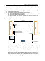
3.3 Spooling machine traverser control with SINAMIC ....................................................... 53
3.3.1 SINAMIC traverser control theory .......................................................................... 53
3.3.2 Traverser control control with PLC&Sinamics strategy based on EPOS function: . 54
3.3.3 Traverser motion profile realized by DCC chart ..................................................... 57
Chapter 4 Simotion controller and its potential in traverser control ..................... 61
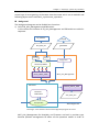
4.1 SiMotion hardware layout ............................................................................................. 61
4.2 SiMotion software layout .............................................................................................. 64
4.2.1 Technological objects ........................................................................................... 64
4.2.2 Program unit ........................................................................................................... 66
4.2.3 Execution system .................................................................................................... 67
4.3 Simotion traverser control concept .............................................................................. 70
Chapter 5 Traverser control by Simotion ................................................................. 72
5.1 Hardware configuration of the Simulation machine ..................................................... 72
III
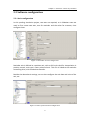
5.2 Software configuration .................................................................................................. 77
5.2.1 Axis configuration ................................................................................................. 77
5.2.2 PLC program block ............................................................................................... 78
5.2.3 Simotion Program Units overview: ..................................................................... 79
5.3 Simotion core program unit .......................................................................................... 84
5.3.1 Axis motion control program unit ....................................................................... 84
5.3.2 Cam profile management program unit.............................................................. 87
Chapter 6 Spooling functionality test ........................................................................ 96
6.1 Spooling performance test ............................................................................................ 96
6.1.1 Setting parameters introduction and classification ............................................... 96
6.1.2 Parameters setting in recipe ................................................................................ 98
6.1.3 Import standard Setting parameters .................................................................. 99
6.1.4 Cam profile calculation ....................................................................................... 100
6.1.5 Cam profile parameters measurement in traverser motion trace.................. 101
6.1.6 Coil profile setting parameter verification ....................................................... 109
6.2 Parameter variation test ............................................................................................. 113
6.2.1 Spooling test with variable calculation mode .................................................. 113
6.2.2 Theoretical analysis for cam profile variable change ...................................... 116
6.2.3 Theoretical analysis for calculation mode change ........................................... 119
6.2.4 Spooling test with fix calculation mode ............................................................ 126
Chapter 7 Concluding remarks ................................................................................ 131
7.1 Conclusion ................................................................................................................... 131
7.2 Project proposal .......................................................................................................... 131
Bibliography.............................................................................................................. 133
IV
List of Figures
Figure 1-1
Figure 1-2
Figure 1-3
Figure 1-4
Figure 1-5
Figure 1-6
Figure 1-7
Figure 1-8
Figure 2-1
Figure 2-2
Figure 2-3
Figure 2-4
Figure 2-5
Figure 2-6
Figure 2-7
Figure 2-8
Figure 2-9
Figure 2-10
Figure 2-11
Figure 2-12
Figure 2-13
Figure 3-1
Figure 3-2
Figure 3-3
Figure 3-4
Figure 3-5
Figure 3-6
Figure 3-7
Figure 3-8
Figure 3-9
Figure 3-10
Figure 3-11
Figure 3-12
Figure 3-13
Figure 3-14
Figure 3-15
Figure 3-16
Figure 3-17
Doctor machine DOC 100.................................................................................... 4
Semiautomatic Slitting and rewinding machine RA2 .......................................... 5
Automatic unwinder AP190 ................................................................................ 6
Range of tightness in different winding approaches ........................................ 12
Two tension zones slitter/rewind ...................................................................... 14
Three tension zones converting machine ......................................................... 15
Layout of Dancer tension control system.......................................................... 16
Layout of Load cell tension control system ....................................................... 17
Layout of spooling machine SP2 ....................................................................... 20
Spooling machine SP2 ....................................................................................... 20
Spooled product................................................................................................ 21
Two types of pineapple winding ....................................................................... 22
Overlap (left) & underlap (right) in spooling..................................................... 22
Positive and negative stagger wind................................................................... 24
Final product of step wind spooling .................................................................. 25
Traversing cycle and its parameters .................................................................. 26
Traverser Motion profile ................................................................................... 27
Spike defined as additional velocity .................................................................. 29
Spike defined as position offset ........................................................................ 29
Stroke in traversing ........................................................................................... 30
Traverser velocity profile with additional speed spike ...................................... 30
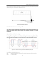
Structure and elements of PLC.......................................................................... 33
Motor starter as actuator controlled by PLC ..................................................... 34
Central process unit of PLC ............................................................................... 35
‘And’ & ‘Or’ logic represented by different programming language ................. 36
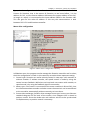
SIMATIC Manager Project Tree structure .......................................................... 38
PLC Scan process ............................................................................................... 39
PLC cycle time ................................................................................................... 39
PLC motor control layout .................................................................................. 41
Motor control with SINAMICS S120 .................................................................. 43
Layout of SINAMIC S120 system ....................................................................... 44
Velocity feed-back control in Control unit ........................................................ 45
Torque compensation for velocity control in Control unit ................................ 46
Current control in Control unit.......................................................................... 47
Pilotage of phase voltages by means of PWM modulation .............................. 48
Description of control parameter quoted from the manual of S120 ................ 48
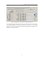
Expert list in Control unit .................................................................................. 49
Traverser Motion profile ................................................................................... 53
V
Figure 3-18 Settings page in the Standard Sinamics traversing control application ............ 58
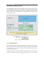
Figure 4-1 SiMotion software control layout ..................................................................... 64
Figure 4-2 SiMotion execution system task level ............................................................... 67
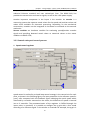
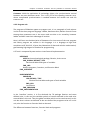
Figure 5-1 Overview of the Simulation machine ................................................................ 72
Figure 5-2 Hardware configuration of the Simulation machine ......................................... 73
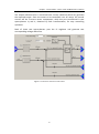
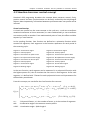
Figure 5-3 PLC rack configuration....................................................................................... 74
Figure 5-4 Configuration of the connection between PLC and Simotion controller .......... 74
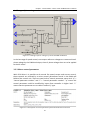
Figure 5-5 Motor drive configuration summary ................................................................. 75
Figure 5-6 Configuration connection between telegram and expert list ........................... 76
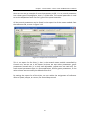
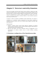
Figure 5-7 Rewinder TO axis configuration ........................................................................ 77
Figure 5-8 Axes synchronization configuration .................................................................. 77
Figure 5-9 Traverser control FB & Cam calculation FB synchronization time diagram....... 95
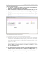
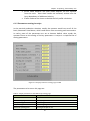
Figure 6-1 Basic setting page on HMI................................................................................. 96
Figure 6-2 Recipe parameters setting page on HMI ........................................................... 98
Figure 6-3 Position and velocity chase of the traverser ................................................... 102
Figure 6-4 Waiting angle measurement, quoted from Sinamics traverser control manual
....................................................................................................................................... 107
Figure 6-5 Acceleration distance measurement, quoted from Sinamics traverser control
manual .......................................................................................................................... 107
Figure 6-6 Winding step measurement, quoted from Sinamics traverser control manual
....................................................................................................................................... 108
Figure 6-7 Three types of coil profile in production......................................................... 109
Figure 6-8 Edge position variation with Reel diameter .................................................... 111
Figure 6-9 Acceleration and waiting angle variation with material layer......................... 115
Figure 6-10 Total angle and total width variation with material layer ............................... 116
Figure 6-11 Total angle & Total width variation with traversing cycle in Setpoint mode ... 129
VI
List of Tables
Table 1-1 Reference of tension by TAPPI for materials ...................................................... 14
Table 2-1 Web material range for spooling machine SL2 and SP2 ..................................... 19
Table 3-1 telegram 105 data structure ............................................................................... 50
Table 5-1 Preset values for cam profile settings................................................................. 87
Table 5-2 Parameters communication between PLC and Simotion ................................... 93
Table 6-1 Input parameters in the HMI basic setting page ................................................ 97
Table 6-2 Input parameters in the HMI recipe setting page .............................................. 98
Table 6-3 Standard recipe setting derived from SP2 spooling machine ............................. 99
Table 6-4 Basic settings converted from recipe for the test............................................... 99
Table 6-5 Polynomial factor in 16 segments of cam profile ............................................. 101
Table 6-6 Measurements of actual setting parameters and comparison with their set
values ............................................................................................................................ 106
Table 6-7 Comparison of settings deviation between Simotion and Sinamics traverser
control ........................................................................................................................... 108
Table 6-8 End position A&B variation when coil angle present ....................................... 110
Table 6-9 Cam profile parameters variation with material layer...................................... 114
Table 6-10 Parameter variation in Setpoint Calculation mode .......................................... 127
VII
List of drawings
Drawing 3-1
Drawing 3-2
Drawing 3-3
Drawing 3-4
Drawing 3-5
Drawing 3-6
Drawing 4-1
Drawing 4-2
Drawing 4-3
Drawing 5-1
Drawing 5-2
Drawing 5-3
Drawing 5-4
Drawing 5-5
Drawing 6-1
PROFIBUS DP communication system ........................................................... 40
Drives communication with telegram............................................................ 51
Complicated synchronization between two motor axes ............................... 54
Speed error due to control interval in Sinamic motor control....................... 55
Speed error due to transmission delay in Sinamic motor control ................. 57
DDC Chart functionality ................................................................................. 57
SiMotion hardware layout ............................................................................. 62
Technological Object link with Expert list by telegram .................................. 65
Traverser axes synchronization through cam................................................. 71
FBLineAxis Block IO overview ........................................................................ 82
Axis motion control unit background program structure .............................. 85
Parameter validation process in motion task 1 of ST_Trav_Traverser ........... 88
Cam calculation functionality in motion task 2 of ST_Trav_Traverser ........... 89
Traverser control unit background program structure .................................. 92
System behavior between two system remedies ........................................ 124
VIII
Introduction
Introduction
Since June 4th, I initiated an internship in IMS Deltamatic Company, an Italian
company has over 50 years history in designing and manufacturing customized
machinery for the converting field.
IMS Deltamatic Company has 5 divisions in products, ‘IMS’ division is for
manufacturing of Converting machine, ‘Deltamatic’ division is for producing
automotive interior, ‘Turra’ is for making plastic injection, and ‘Rotomac’ division
for packaging, ‘Kasper’ for machine tools.
I worked in ‘IMS’ division, this division produces mainly the following types of
machines:
1. Slitter-Rewinders that covers wide range of web sizes and rewind typologies;
2. Inspection-Rewinders and doctor machines either mono or bi-directional;
3. Automatic non-stop rewinders for flying reel-change at high-speed, featuring
either center or surface drive;
4. Automatic non-stop unwanders for flying splice, featuring either overlapped,
or butt or register splice type;
5. Doubling and separating machines for aluminum foil and strip;
6. Embossing machines for aluminum foil;
7. Spooling machines.
In this internship my study mainly focused on the programming for automation
process. Through this internship I have acquired basic concepts of automation
control, both in hardware and software aspects: I got knowledge on the
communications between machines and their control master with Profibus; I
have learned to use different categories programming languages to realize an
logic control for the automation process with PLC; I have learned how the
position and velocity control are realized in electric motors with Sinamic: I have
learned the skill to design a HMI operating panel with WinCC: Most importantly I
have studied Simotion, a new control system dedicated for the motion control of
motors, I got the ability to write program for it and made communication
between it and other devices.
1
Introduction
Based on what I had learned, at the middle time of the internship I undertook a
project aiming to reform the control methodology of the traverser in spooling
machine, changing from the traditional method realized by Sinamic to a new one
adopting Simotion control system. Thanks to my colleague Andrea and
Valentino’s previous work on Simotion I was able to control the multi axis of
electric motor and realized their synchronization using the well-developed
program unit.
Firstly, I developed a program unit dedicated on regulating the cam profile
between two synchronized axes, with which the movement of the traverser can
be characterized by setting user desirable parameters. After that I designed a
testing operation panel from which the assignment of parameters and the
reading of system output could be very convenient, thus to ease the performing
of test process. In the test my efforts are put on the verification of the accuracy
and stability of my program system, more specifically, to see if the actual
measured parameters are equal to the settings, to see whether the variation of
the actual parameters could cause a failure of the system, also I test the
relationship between the system variables, to understand the basic working
principle of the library program offered by Siemens. The test went well, finally I
adopted my program unit with the Company standard, to realized the logic
control from PLC side and motion control dedicated by Simotion.
This thesis proceeds as follow, the introduce of some basic principles about the
converting machine is made firstly, since spooling machine is converting machine
with special functionality, then the spooling machine with its special
functionality would be decribed. Secondly I will demonstrate how the
automation control is made with PlC, Sinamic and Simotion. And at last my
project about the traverser control is to be introduced.
2
Chapter 1 Converting machine overview
Chapter 1 Converting machine overview
1.1 Introduction of converting machine
A converting machine includes all of those devices that execute a process of
unwinding and rewinding on a bobbin. These machines have functionality of
transporting the web firstly and then make it pass from one bobbin to another with
different features such as diameter and width. In this small chapter are introduced
the objective of converting machine, the property of its final products and a brief
grant of IMS Deltamatics Spa’s converting machines.
1.1.1 Objective of converting machine
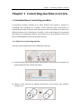
Generally converting machine have 3 objectives, they are:
a) Produce bobbin with reduced width and diameter from a mother reel which has
greater dimension for economical reason.
b) Works on the material for adding characteristics like printing, coat, emboss,
laminate, etc.
3
Chapter 1 Converting machine overview
c) Rewinding a bobbin to eliminate roll defects, like offsets, telescope, soft rolls.
1.1.2 Products of converting machine
The material of final product for converting could be paper, plastic and aluminum,
the thickness of web can vary from several micrometers to millimeters. Due to the
versatility of the converting machine, its final products could be used in many
industrial domains, for example packing, automotive, cigarette production etc.
1.1.3 IMS machines Presentation
In IMS Deltamatic Corporation several types of converting machine are produced,
they could be divided into: Doctor machine, Slitting and rewinding machine, Winders
and Unwinders.
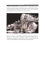
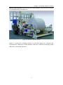
Doctor machine: They are machine for the purpose of controlling the defects, they
can eliminate the material defects or the part non desirable.
Figure 1-1 Doctor machine DOC 100
Above is a picture for doctor machine DOC 100, it can deal with bobbin with a
maximum diameter 1000 mm and maximum width 500 mm, it has a maximum
working speed 300 m/min.
4
Chapter 1 Converting machine overview
Slitting and rewinding machine: This type machine uses circular cutters to slit the
jumbo roll and rewind them into several smaller rolls. It is completed with hydraulic
roll lifting, photoelectric auto-error correction system, tension controller, automatic
meter-counting, PLC-controlled machine operations. It can be used for slitting and
rewinding paper, adhesive paper, plastic film, aluminum foil, etc.
Figure 1-2 Semiautomatic Slitting and rewinding machine RA2
Above is a picture for a semiautomatic slitting and rewinding machine RA2, it is
dedicated in paper process. Characteristics: Maximum unwinding diameter
1200/1800 mm, Maximum rewinding diameter 1200 mm, maximum speed 1200
m/min, web width 1000/2500 mm, minimum web cutting width 100 mm.
5
Chapter 1 Converting machine overview
Winders and Unwinders: Machines wind or unwind bobbin, they are part of a line of,
for example printing, laminate, etc.
Figure 1-3 Automatic unwinder AP190
Above is a picture for Unwinder AP190, it is the final station of a printing line.
Characteristics: Maximum unwind diameter 1950 mm, maximum processing speed
800 m/min, web width 1650 mm.
6
Chapter 1 Converting machine overview
1.2 Concepts about winding process
Winding is an importing process in the converting machine, at the beginning a
unwinding process on the mother reel to feed the machine with material web,
after the main process such as slitting or printing the web is rewound into a new
bobbin with different diameter or web width. Therefore the study of winding is
necessary to obtain perfect final product. In this small chapter are introduced the
definition and the benefit of winding, different types of winding types and the
variables in the winding process.
1.2.1 Winding definition
Winding means material (as wire) wound or coiled about an object or the action
to make it. Therefore ‘To wind’ is to encircle or to cover with something pliable.
Similarly, ‘unwind’ means to remove from tension, to uncoil to wind off material.
1.2.2 Purpose of winding
Winding is a process of turning flat stuff into round stuff, for its 3 advantages, the
most import one is that, looking from engineering aspect, round stuff could store
more material in smaller space. Moreover, it could protect them from folding or
cutting. The last one from aesthetics points of view, round stuff looks pretty.
1.2.3 Winding variables
Roll hardness is developed in different ways on different types of winding classes.
However the basic principles of how to build roll hardness are always the same.
Three key variables can be defined to describe the hardness of final bobbin, they
are: the tension in the material web, the pressure on the surface on the bobbin,
calling nip, and the difference of the moments applied between the axis of
bobbin and the supporting roller, calling torque. These three variables are short
for TNT (Tension, Nip, Torque), they are fundamental factors not only because of
their contributions to the tightness of bobbin individually, but also because they
can be controlled separately.
7
Chapter 1 Converting machine overview
Tension
Tension of the material web is defined as the force applied at unit of width, the
unit of tension is in [N/m], or sometimes simplified as [N], this is the parameter
affects most the compactness of the final bobbin. For some types of material or
some processing zone, keeping a constant tension is also important to guarantee
no defect on the final product.
The tension can be controlled by several methods, such as dancer and load cell,
they are close-loop control methods and can maintain the tension effectively.
Nip
Nip is the load applied on the line of contact, between the outer surface of the
bobbin and the roller, it is measured in [N/m]. This load is able to avoid the air
from slipping into the bobbin causing defects like telescope, especially for the
material porous. Generally the Nip is controlled by a system of oleodynamic
actuator.
Torque
Difference of moment acting on two roller motorized is the third variable, torque.
This parameter is controlled by the electric drives, by modifying the current in
the motor circuit it can introduce a difference of velocity, resulting as difference
in moment due to the characteristic curve of electric motor.
Wound-In-Tension
The effect of the previous 3 parameter is to make the bobbin tight, their effect
can form a combination resulting on a single parameter called Wound-In-Tension,
WIT in short, describes the extend of compactness resulting after a certain
winding process, it could be measured in [MPa].
After the study of the contribution of Nip to WIT conducted by Pfeiffer, a formula
is obtained:
WIT =
1
𝑁+𝛼
𝑇∙𝑁
∙ 𝑙𝑜𝑔 (
) +
𝛽
𝛼
𝛾+𝛿∙𝑁
N = Nip (PLI)
T = Tension (PLI)
𝛼, β, γ, δ = Coefficient
In the winding process it is common to convert the effect of torque into web
8
Chapter 1 Converting machine overview
tension so only consider with tension and nip, so in this case WIT is only a
function of Nip and Tension, the contribution of these two variables depends on
the property of the material, especially the compressibility. Material soft like
cloth is highly influenced by Nip, while material like aluminum and paper are
affected less. Then according to Good’s research, he found a relationship simpler
between WIT and TNT:
WIT = T +
𝜇∙𝑁
10 ∙ 𝐶
WIT = Wound-In-Tension [MPa]
T = Tension
𝜇
= material coefficient
N
C
= Nip [N/cm]
= material thickness [mm]
In industrial production this law provides a useful quantitative indication for the
effect of processing variables on final product.
Effect of Wound-in-Tension
Wound-in-Tension is the most important factor in determining the difference
between good quality and poor quality rolls of film products. Rolls that are
wound too soft will go out of round while winding or will go out of round while
being handled or stored. The roundness of rolls is very important in customer’s
operation. When unwinding out of round rolls, each revolution will produce a
tight and slack tension wave. Theses tension variations can distort the web and
cause register variations in the printing process. The only way to minimize the
effect of these tension variations is to run the operation at a much lower speed,
which greatly affects the production efficiency.
Rolls that are wound in too high WIT will also cause problems. Rolls of some films,
when wound too tightly will introduce roll blocking, this is a defect where the
sheet layers fuse or adhere together. When winding extensible film on thin wall
cores, winding hard rolls can cause the cores to collapse. This can cause problem
in removing the shaft, or with inserting the shaft or chucks on the subsequent
unwinding operation. Tightly wound rolls contain high residual stresses. The film
will stretch and deform as these tresses are relieved as the rolls cure during
storage.
Moreover, rolls that are wound too tightly will exaggerate web defects. No web is
perfectly flat or the same thickness from one side to the other. Typically, webs
will have slight high and low areas in the cross machine profile where the web is
thicker or thinner. When winding hard rolls of film, the high caliper areas build on
9
Chapter 1 Converting machine overview
each other. As thousands of layers are wrapped creating a roll, the high areas
form ridges or high spots in the roll. As the film is stretched over these ridges, it is
deformed. Then when the roll is unwound, these areas produce a defect known
as bagginess in the film. Hard rolls that have high gauge bands next to low gauge
bands will produce a roll defect known as corrugation or rope marks in the rolls.
1.2.4 Winding classes
To coil the material on a core, three classes of winding are available in the
industrial manufacturing.
Center winding: The shaft which supports the core is driven directly by a motor,
the motor provides the coil with torque control or velocity control to realize the
winding process.
In center winder only tension is used to control the roll’s hardness. A center
winder could also incorporate a lay-on or pressure roll. This winder wound use
both tension and nip to control the roll’s hardness. With a center winding process,
the spindle torque through the center of the roll provides the web tension.
An advantage of center winding is that this process can wind softer rolls. This
type of turret winder can provide quick indexing and fast cycle times. The
disadvantage of center winding of film is the limitation of maximum roll diameter
due to the torque applied through the layers of film. Also, center winder has a
higher probability of generating scrap during roll changes.
As conclusion, center winders are best for winding soft rolls (i.e. films with gauge
bands), winding for film with high tack, winding for small diameter rolls, it is
easily designed for dual direction winding and able to provide adhesiveless
transfers.
Surface wind: Similar to center wind with lay-on roller, but the center shaft is
free of load while the Lay-on Roller is driven, the lay-on roller drives the coil to
wind by friction.
When surface winding is applied on elastic films, web tension is the dominant
10
Chapter 1 Converting machine overview
winding principle. When surface winding inelastic materials, nip is the dominant
winding principle. Surface type film winders use a driven winding drum. The
winding rolls are loaded against the drum and are surface wound.
The advantage of surface winding is that the web tension is not supplied from
torque being applied through the payers of film wrapped into the roll. The
disadvantage of surface winding of film is that air cannot be wound into the roll
to minimize gauge bands and roll blocking problems.
Surface winders are best for winding hard rolls (i.e. protective films), best for
utilization of space and horsepower, best for winding very large diameter rolls
and minimizing waster during transfers, also it is less expensive.
Center-Surface winding: A center-surface winder uses both center winding
and surface winding methods, it uses all of the three variables in winding process:
TNT. The web tension is controlled by the surface drive connected to the lay-on
roller to optimize the slitting and web spreading processes. The lay-on roll
loading applied to the winding roll controls the Nip. The Torque from the center
drive is programmed to produce the desired WIT for the roll hardness profile
desired.
The advantage of center-surface winding is that the winding tension can be
independently controlled from the web tension. While its disadvantage is the
winding equipment is more expensive and more complex to operate.
Center-surface winders are best for winding high slip films or slitting and winding
extensible films to larger diameter, it is able to supply WIT without stretching the
web over caliper bands.
Since different winding classes realize the winding process in different
methodology, they provid the coil different range of tightness, which has the
same meaning as WIT. Following is a figure to illustrate the range of tightness
provided by different winding class.
11
Chapter 1 Converting machine overview
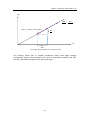
Figure 1-4 Range of tightness in different winding approaches
From the above figure we can see, Center wind provides the tightness range from
minimum to maximum, with the lay-on roller addition tightness is added. Surface
winding can’t get as loose because of required nip. The center-surface winding
provides the widest range.
12
Chapter 1 Converting machine overview
1.3 Tension control
Tension is a parameter should be carefully controlled during the converting process,
since its effect on the quality of the final product is negligible. Different material
webs have different requirement for working tension, moreover, a proper tension
depends also on the working zone undertaking different types of process. For
example the unwinding process requires a tension with medium value, being
sufficient to regulate the supply and alignment of the web. While in the intermediate
machine zone where the web is undertaken the coating, a lower tension is needed.
On the contrary, in the final zone of rewinding process, a higher tension is necessary
to assure the compactness of the final bobbin. Due to this reason tension control
techniques are introduced into the converting machine. In this small chapter, we will
talk about the method to find optimal tension for process and how the division of
tension zone is realized in converting machine, also two important techniques of
tension control.
1.3.1 Optimal tension for processing
There are several methodologies to find out the optimal tension for processing, one
of the most useful is the method based on experiments. For the same material,
experiments are taken by varying the tension subjected by the web, then find out
with which tension the machine could obtain best products. This value becomes the
standard. So this tension could be used also for the material which has similar
property after modification. Since the tension is linear with thickness, the new value
should be recalculated with consideration of the ratio between the thickness of the
present web and that of the standard web.
For the case undertaking experiments is impossible, general rule of thumb is that the
best tension is equal to 10% to 25% of the tensile strength of the material.
Another alternative is that to use the suggest tension value provide by technical
organization such as TAPPI (Technical Association of the Pulp and Paper Industry),
which publishes estimated proper tension levels for many types of materials and
laminates. Following is a table providing reference value for some materials.
13
Chapter 1 Converting machine overview
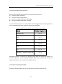
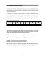
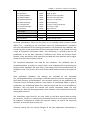
Table 1-1 Reference of tension by TAPPI for materials
Material
Tension
[lbs./inch/mil]
Polyester
0.5 to 1.5
Polypropylene
0.25 to 0.5
Polyethylene
0.1 to 0.25
Polystyrene
0.5 to 1.0
Vinyl
0.05 to 0.2
Aluminum Foils
0.5 to 1.5
Cellophane
0.5 to 1.0
Nylon
0.10 to 0.25
1 lbs./inch/mil = 7.03 kg./cm/mm
1.3.2 Division of tension zone
A tension zone in a web processing machine is defined as that area between which
the web is captured or isolated.
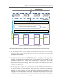
How to realize the division of tension zones? Let’s see the common example in a
simple slitter/rewinder below:
Figure 1-5 Two tension zones slitter/rewind
14
Chapter 1 Converting machine overview
In this case, there are two separate tension zones to deal with and the tension levels
may be different in each zone. Different tension levels are possible due to the fact
that the web is captured at the driven nip rolls (also ‘Pull unit’), thus creating
separate and distinct unwind and rewind zones if the nip exceeds the critical value.
The driven nip rolls will typically be powered by a motor drive that establishes
machines line speed.
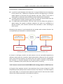
As mentioned before, the right tension for working depends not only on the material
but also on the process, in a converting machine it can be divided into 3 processing
zone: unwinding, intermediate processing, rewinding. Therefore 3 different tension
zones should be created in the converting machine, each one has its own proper
value on tension. So the proper structure for the converting machine would be:
Figure 1-6 Three tension zones converting machine
In this case, one of the intermediate zone drives will typically establish line speed,
and the control of drive rolls for the other zones will relate to this drive. In some
instances, a simple master/slave relationship with a speed differential ratio will
provide the draw tension necessary in that zone. While in common case, the tension
control is accomplished with closed loop trim (dancer or load cell).
1.3.3 Closed-loop tension control: Dancer and Load cell
Closed loop tension control systems provide very precise and accurate tension
control during steady state running conditions as well as acceleration, deceleration
and E-stop(Emergency stop) conditions, because the change of tension are detected
immediately and the controlled device is changed instantaneously to maintain
accurate tension control.
15
Chapter 1 Converting machine overview
The two most common methods of closed loop tension control are dancer and load
cell.
Dancer
There are many different designs of dancer roll tension controls. However, all dancers
operate with a common principle. They all incorporate idler rolls that are ‘loaded’ in
one direction, while the web tends to move them in the opposite direction. These
rolls are supported by pneumatic actuators who provide reference of force which can
convert to web tension by calculation. A sensor detects the position of the dancer
and tells the drive to increase or decrease in speed or torque to add or remove
material from the dancer. As long as the dancer roll remains between its physical
limits (completely empty or completely full) tension is constant on the web.
Following is a figure for the layout of dancer.
Figure 1-7 Layout of Dancer tension control system
Using Dancer to control the tension has many advantages, the most important one is
that the dancer has some amount of web storage. This means it accumulate a certain
length of web in the machine direction, when tension fluctuations due to splices,
defective bearings or other factors occur, dancer can absorb it. In this way, dancer
not only controls torque and line speed to keep tension constant, it also absorbs
tension fluctuations, so web tension downstream of the dancer is kept smooth.
Dancer has also some disadvantages. The control reference is not the web tension
directly but feedback in geometric variables, thus will cause phase delay in the
control, which would probably render the system become unstable. The dancer takes
larger space in the machine.
Load cell
Similar with Dancer, in load cell control system a idler roller also exist to support the
web, while load cell tension controls utilize strain gauges and other weight
16
Chapter 1 Converting machine overview
measuring devices to measure the load applied to the idler roller due to web tension.
The force exerted to the idler roll is proportional to the tension and the wrap angle
around the roll. The measured signal is feedback to the control system to perform
close loop tension control by altering line speed or torque of the drive. Following is a
figure for the layout of load cell:
Figure 1-8 Layout of Load cell tension control system
After the reference tension is set, measurement signals are generated on both sides
of the idler roll and fed into the control unit. The control accepts both signals and
processes them together. Process values and set values are compared and an output
is generated and sent to the drive to keep tension constant.
Load cell is able perform an excellent and accurate tension control at the unwind
rewind and intermediate zone since its directly feedback of tension signal, moreover,
it is relatively inexpensive and easy to install respecting to dancer, so minimal
machine modifications are necessary to utilize this control.
However since there is no storage for material, it has no ability to absorb tension
fluctuations.
17
Chapter 2 Spooling machine overview
Chapter 2 Spooling machine overview
After the introduction of converting machine in chapter 1, we know that in
converting machine we can remake web material from large bobbins to smaller
bobbins, both in diameter and width. When smaller web width is required, it is
necessary to slit the web in intermediate processing zone, thus to create a series of
pancakes.
However, as the web width is narrow, when material web is wound as a pancake the
length of material is restricted due to the instability of the final wound package. The
limited web length is a problem for many products manufacturing activities, such as
cigarette, food package, personal care, aerospace etc. Without sufficient length,
number of times need to change the mother bobbins is higher, the process meets
more interrupts during production, thus lower the efficiency and productivity.
A solution to increase the web length of narrow film is to introduce the spooling
technique, the machine in charge of spooling operation is a spooling machine. In this
chapter, I will give introduction of spooling machine and important principle about
the spooling technique.
2.1 Introduction of spooling machine
Spooling machine is one of the important product of IMS DELATAMATIC SPA, in this
small chapter will be introduced the how is the spooling machine produced by IMS,
how does it work and what’s its characteristic.
2.1.1 Description
The spooling machines of IMS DELTAMATIC SPA are available in two different models
in order to combine the most suitable technology according to the material to be
processed: SL2 model can hold the strips in position and shuttle the rewind shafts
back-and-forth to form the spools, while SP2 model works in the opposite way by
traversing the strips and keeping the rewind shafts stationary.
Both these two models allow up to 24 spools and feature a dedicated software
program designed for an extremely fine interface between the different motors, so
as to enable shaping the spools with the best desired configuration(amount of
overlap between strip, waiting angle, etc.)
18
Chapter 2 Spooling machine overview
2.1.2 Characteristic of the machine
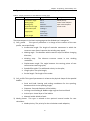
There are four typical final products for these spooling machines:
Yarns for textile industries
Yarns for technical applications
Very narrow web products for packaging
Very narrow web plastic films for tapes
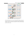
As to the web materials, it is illustrated in the following table the working materials
and corresponding thickness range for these spool machines.
Table 2-1 Web material range for spooling machine SL2 and SP2
Material
Thickness range (μm)
Aluminum Foils
20 - 70
BOPP
18 - 50
CPP
18 - 50
PET
12 - 50
HDPE
20 - 60
PVC
20 - 60
Laminates or Multilayers plastic film
30 - 60
Standard technique characteristics: Working width 600 mm, Maximum mother roll
diameter 1000 mm, max rewinding diameter 400 mm, the maximum mechanical
speed is 300 m/min, the minimum slit width is 5 mm.
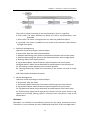
2.1.3 Layout of spooling machine
From the Following figure we can see the layout of spooling machine SP2:
19
Chapter 2 Spooling machine overview
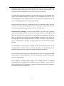
Figure 2-1 Layout of spooling machine SP2
In the machine of IMS DELTAMATIC SPA, the spooling concept is slitting and spooling
on one machine. The machine is in two parts, the unwind/slitter on the left part and
the spooler on the right side. In the first part, the mother roll is loaded into the
unwind with the web passing through a slitting station where it is slit to the final web
width, then these webs pass through the traverser and fanned out to multiple
spooling station.
Slitting and spooling in one process eliminates the extra handling necessary when
slitting first and then spooling as a separate operation and is the preferred method
for higher volume operations.
Following is the figure for the spooling machine SP2
Figure 2-2 Spooling machine SP2
20
Chapter 2 Spooling machine overview
2.2 Principle of spooling
The idea of spooling is to wind narrow film into a bobbin which has a larger width
than the film, by distributing the web homogenously on the shaft. A brief
introduction about the principle of spooling will be given in this small chapter.
2.2.1 Definition
Here are listed some definition of terminology in the spooling technique.
Spool: A spool is a package of material which is
much wider than the material that has been
wound. Typically, it has been wound using a
traversing method, this allows the material to
be overlapped or under lapped during the
winding process.
Spooling: Spooling, Traverse Winding, Level
Winding. All these terms are used to depict the
Figure 2-3 Spooled product
principle of winding a tape having narrow
widths into a spooled package to create a continuous longer length, with which the
pancake could then be easily transported and handled in their final application.
In order to realize the spooling of material web, generally two methods are adopted.
One is synchronize the normal winding process with a traversing process of the
traverser, which is a traversing arm guiding the horizontal position of the web. The
other is to traverse the winding shaft itself in the winding process.
Tape width: The width of the material to be spooled or traverse wound.
Spooled width: The width of the finished spool when wound onto the core.
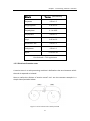
Pineapple winding: Pineapple shape of winding will form as reducing the width of
the spooled package as each layer is wound. This spooling shape is used when
processing certain material, or thick material i.e. greater than 1 mm, additional
support to the material at the ends is necessary.
21
Chapter 2 Spooling machine overview
Figure 2-4 Two types of pineapple winding
Overlap: When winding a narrow width tape, if it is wound with 100% overlap then a
pancake is created. As we reduce the degree of overlap, the principle of spooling
comes into its own. When one layer of material covers the preceding layer of
material, the percentage of covered part is the amount of overlap.
Underlap: When traverse winding a package, if one layer does not overlap the
preceding layer, but leaves a gap between it, then this is said to be winding with an
underlap or negative overlap.
Figure 2-5 Overlap (left) & underlap (right) in spooling
Lobbing: It is the points at the end of the spool where the material reverses direction.
When creating a lobed package, the position of reversal is calculated mathematically
and retained in exactly the same position throughout the production of the spool.
Imagining a four lobed package, this would mean on one side of the spool there
would be four points for reversal, for example, 12 o’clock, 3 o’clock, 6 o’clock and 9
o’clock and at the opposite side of the spool the reversal points would have a phase
shift of 45 degree.
Dwell: Also called waiting angle, it is the waiting time (In ‘degree’ of the winding
shaft’s rotational movement) between before and after changing traversing
22
Chapter 2 Spooling machine overview
direction.
When processing compressive, thin material it is often advantageous to create a
dwell at the end of the traverse. Thus increases the amount of material at the end of
the spool and, therefore, creates a denser package at this point. When processing
thin foam or non-woven materials the introduction of a dwell at the end of the spool
gives greater stability to the finished package. These dwells can vary from a few
degrees to hundreds of degrees, depending on the particular type and width of
material being processed.
2.2.2 Different spooling approaches
Several spooling approaches could be adopted for the spooling processing, each of
them is suitable for specific material or web width, for certain advantage.
Level wound spools
Level winding is to form a spool by traversing the material across the face of the core
and, at the appropriate time, reverse its direction so the material traverses in the
opposite direction, thus building up a number of layers until a finished spool is
created. This is the most common spooling style.
In this spooling approach, the edge of the spool is the most vulnerable point and it is
of paramount importance that anyone handling the spool does not press the side as
it will cause damage to this product. This is a particular problem if the material is
adhesive, as the layers of material that protrude at the end of the spool will then
adhere together and create a problem during the de-spooling process. To optimize
the efficiency of de-spooling, it is important that the equipment used is designed for
the de-spooling the particular product being unwound.
Stagger wind
The principle of stagger winding is to increase the amount of material at the
turnaround point of the reel to reduce the effect of creating a cambered rewound
spool. This principle is particularly useful when processing extremely narrow width
material (in the region of 0.2 mm wide). Typically, one could set up the equipment to
create a stagger distance of x mm, relative to the width of spool being wound and
the number of layers before a stagger layer is introduced.
23
Chapter 2 Spooling machine overview
Figure 2-6 Positive and negative stagger wind
TM
Stepped-Ends
This winding technique is a KT Industries Patented spooling technique when the
dwell at the end of the stepped end package is greater than 720° enable an
overlapped spooled package to be created with solid ends. Essentially, it is a
combination of a pancake and a spool. When spooling product, the end of the
package is vulnerable to damage due to the interleaved edges of the material at the
end of the spool. The basic principle is to create a pancake at the end of the spool
providing protection and then to conventionally spool between the pancakes but
create a longer length. This technique significantly reduces the distortion created
from a level wound spooling product. This principle of spooling is particularly
beneficial when processing a thin product.
Step Wind
A step wound reel is a reel which is a combination of a pancake and a spool. The
principle is to wind the material for a given number of revolutions and then traverse
the material to the next position for winding again. The layers which have been
wound in the fixed position are creating a pancake and then by traversing to the next
position and leaving a gap, the next pancake wound. This principle is repeated the
full width of the core until ending up with a number of pancakes wound next to each
other. The multiple pancakes then give support to each other and, therefore, reduce
the possibility of telescoping.
The step wound spool has a number of advantages over the conventional traverse
wound spool:
The package density of step wound spool is normally much greater than the density
of the standard level wound spool due to the reduction in overlap of the material.
The higher density means more material is provided in the same volume. Moreover,
this way of spooling increases the stability and reduces the vulnerability of the final
product due to the pancake type wind. Also, during high speed payout the tape is not
24
Chapter 2 Spooling machine overview
subjected to inertial problems at the end of the package as it is unwinding as a
pancake. This minimizes the possibility of the tape dropping off the edge of the spool
during the de-spooling process.
Figure 2-7 Final product of step wind spooling
2.2.3 Spooling benefits
The most important benefit of a spool wound product is the ability to increase the
length of material being presented to the final process. It would be virtually
impossible in many narrow width products to achieve a reasonable length material
without using this technique. Large material length can reduce significantly the down
time of the final process.
Besides, Spooling has Advantage such as the reduction in the possibility of removing
the core from the finished reel due to slippage, since the spooled width of material is
far greater than that of a single pancake wound material.
During the spooling process, the tension requirements of a spooled product are
much less than those of a pancake wound material, therefore, the distortion due to
elongation is reduced.
As to the de-spooling process, since the material itself is held together on the spool
by the spooling action, when de-spooling the ability to control the unwind tension is
far easier and also the build-up ratio from outside diameter to inside diameter is
much less and, therefore, more controllable.
25
Chapter 2 Spooling machine overview
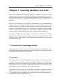
2.3 Traverser motion profile
Traverser is a device guiding the distribution of the material web on the winding core,
it moves between the starting point and the ending points of the traversing process,
surely its moving characteristic would affect the distribution of the material, affect
the shape of the final spool, therefore it would affect the quality and stability of the
final product. Due to this reason, a study of the motion profile is necessary.
2.3.1 Principle of operation
In traversing operation, the traverser (traversing arm) moves between the edges of
the coil being wound. The absolute position of the traverser is synchronized with the
relative position (angular offset or displacement) of the winder during this cycle.
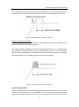
Figure 2-8 Traversing cycle and its parameters
In this diagram are shown one traversing cycles to demonstrate the mode of
operation and the important parameters of the traverser. During the description, all
angular data refer to the angle of the winder shaft:
Acceleration angle [deg] : In the acceleration angle, the traverser is accelerated from
standstill up to the synchronous velocity, or decelerated from the synchronous
velocity down to standstill.
Waiting angle [deg] : Also called dwell, the waiting angle defines the angle which the
traversing axis is at stand still at one end points of the roll being wound before it
moves in the opposite direction. The waiting angle defines the edge that is created at
the end points of the coil being wound.
Displacement angle [deg]: The displacement angle defines the angle between the
starting points of two consecutive traversing cycles.
26
Chapter 2 Spooling machine overview
Winding step [mm/rev]: The feed of the traverser is defined by the winding step,
which defines the feed of the traversing axis during one revolution of the coil being
wound.
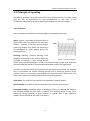
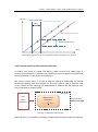
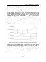
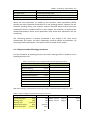
2.3.2 Traverser motion profile
The traverse motion profile include velocity profile and position profile, as shown in
the following figure, black line presents for the actual position of the traverser while
red line presents for its velocity.
Figure 2-9 Traverser Motion profile
Procedure introduction
As seen in the figure, the horizontal axis presents for winder position in degree, the
vertical axis presents for the traverser position [mm] and the traverser velocity
[mm/deg].
From the position profile we can see a complete traversing cycle, the traverser starts
from the left end of the traversing axis with coordinate -10, moves to the right end of
the axis then reaches the end with coordinate 10 before reversing its moving
direction.
Let’s see the velocity profile, at the first half of the traversing cycle, traverser start
with an acceleration angle, in which it increases the traversing velocity until it
reaches the constant velocity decided by winding step.
After its acceleration, traverser experiences a ‘spike’, as its definition, the spike
function is used to control how the material is wound at the edge of the coil as a
result of acceleration or braking, so during the spike, the traverser will traverse in a
27
Chapter 2 Spooling machine overview
velocity slightly higher than the constant traversing velocity, the difference in velocity
is called additional velocity.
After the spike traverser enters a period of traversing movement with a constant
velocity, this period is named FCA (Forward Constant velocity Angle). Before the
traverser reaches its right end, a spike is necessary to modify how the material is
wound at the edge. Then in the next acceleration angle, the traverser’s velocity
decelerates to zero and the traverser reaches in standstill state.
Before the traverser reverses its moving direction, it maintain the state of zero speed
at the edge of the core for a period of time, this period is called waiting angle. As
introduced before in the principle of spooling, a proper waiting angle, or dwell, can
increase the quality of the spool edge.
In the second half of the traversing cycle, the traverser moves from the right hand
end to the left hand end, with the same velocity amplitude while opposite direction.
Therefore the velocity profile in the second half is inversely symmetric with the
velocity profile in the first half.
Spike implementation
The adoption of spike is to control how the material wound at the area near edge of
the coil, since at the period that traverser starts to leave the spooling end, before a
constant traversing web angle is reached, the velocity of the contact points between
the web and the coil is lower than the traverser speed, in order to render the contact
point speed(the actual spooling speed) equal to the winding step, the traverser is
proposed to move at a speed a bit higher than the winding step speed before the
constant traversing web angle is reach. The quantity of this additional speed depends
on the distance between the traverser and the contact points, depends on the
material property of the web, therefore, this additional velocity has a layer
dependency.
Four independent spikes can be parameterized in one traversing cycle, two before
and two after the end of coil points.
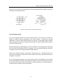
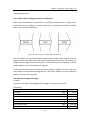
There are 2 modes for defining the spike, one defines with the additional velocity,
the other one defines with the position offset. With different methods we can obtain
different motion profile in the period of spike.
Definition with additional velocity:
In this mode, a spike is defined by the spike length and the additional velocity as in
the figure [fig 2-10]. The spike length is defined in degrees referred to the winding
axis and defines the part of the spike in which the traverser moves with a constant
velocity. The velocity offset is specified in mm/360°.
28
Chapter 2 Spooling machine overview
The acceleration and braking phases of the spike are not considered in this mode.
The acceleration and the deceleration of the spike have the same absolute value as
the acceleration or deceleration of the motion profile at the end points of the coil.
Figure 2-10 Spike defined as additional velocity
Definition with position offset:
In this mode, the spike is defined by the spike length and the position offset of the
traverser displayed in the figure [fig 2-11]
The velocity offset- including the acceleration and deceleration- are calculated from
the specified parameters and cannot be influenced by the user. For the position
offset, a linear interpolation is made between the parameterized points; acceleration
and deceleration can, if necessary, be limited by the axis settings.
Figure 2-11 Spike defined as position offset
Stroke implementation
Stroke is the parameter represents the gap between the end position of the traverser
and the end of the coil, as in the figure [fig 2-12]. The stroke is used to ensure that
the material reaches the end of the coil. This is important since the material cannot
29
Chapter 2 Spooling machine overview
always be traversed vertically to the coil. In order to ensure that the material reaches
the coil end points during traversing, the traverser must move somewhat beyond the
defined end points. The stroke is measured in mm.
Figure 2-12 Stroke in traversing
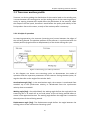
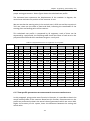
2.3.3 Calculation of traverser motion profile
The traverser motion is defined by the combination of the setting of parameters, this
means the motion profile could be obtain by calculation involving all of those
parameters.
Spike defined as additional velocity
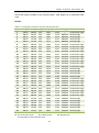
In this typical case, spike is defined as additional velocity in unit [mm/rev], as
knowing the total angle is the sum of all period length in one spooling cycle, and also
the cycle length (Total width) is the total area cover by the speed profile, we have:
Figure 2-13 Traverser velocity profile with additional speed spike
In the figure, the abbreviations are:
AS#
: [mm/rev] additional velocity of the spike, # represents for the number
AS#C
: [°] Spike length
30
Chapter 2 Spooling machine overview
AAS#
AS
ASC
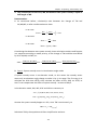
: [°] the acceleration angle of the spike to reach the additional velocity of
the spike, it is calculated from the values of AA, WS and AS#
: [mm/rev] sum of the additional velocities AS#
: [°] sum of the spike length AS#C
The following equations define the motion profile of the traverser:
1. Formula for Total Angle
TA = 4*AA + 2*WA + FCA + BCA + ASC + 2*AA*AS/WS
2. Formula for Total length
For Forward movement:
360*TW = [AA*WS/2] + [(AS1/WS*AA)*WS + [(AS1/WS*AA)*AS1/2] + [AS1C*WS] +
[AS1C*AS1] + [(AS1/WS*AA)*WS] + [(AS1/WS*AA)*AS1/2] + [FCA*WS] +
[(AS2/WS*AA)*WS] + [(AS2/WS*AA)*AS2/2] + [AS2C*WS] + [AS2C*AS2] +
[(AS2/WS*AA)*WS] + [(AS2/WS*AA) * AS2/2] + [AA* WS/2]
For Backward movement:
360*TW = [AA*WS/2] + [(AS3/WS*AA)*WS + [(AS3/WS*AA)*AS3/2] + [AS3C*WS] +
[AS3C*AS3] + [(AS3/WS*AA)*WS] + [(AS3/WS*AA)*AS3/2] + [FCA*WS] +
[(AS4/WS*AA)*WS] + [(AS4/WS*AA)*AS4/2] + [AS4C*WS] + [AS4C*AS4] +
[(AS4/WS*AA)*WS] + [(AS4/WS*AA) * AS4/2] + [AA* WS/2]
31
Chapter 3 Automation control with PLC&Sinamics Products
Chapter 3 Automation control with PLC
& Sinamics Products
In the converting machines, the working processes are done by the machine with a
automation control, from moving the mother reel to the correct position after
loaded, accelerating the roller to preset velocity, approaching the cutting knife to the
web, to stopping the roller when bobbin diameter reach its maximum. But how these
motions are realized? This chapter would focus on the automation control realization
in the converting machine.
3.1 Programmable logic controller
A programmable logic controller is a digital computer used for automation of
electromechanical processes, such as control of machinery on factory assembly lines,
amusement rides, or light fixtures.
Unlike general purpose computers, the PLC is designed for multiple inputs and
output arrangements, extended temperature ranges, immunity to electrical noise,
and resistance to vibration and impact. Therefore, it is very suitable for many
industries and machines.
In IMS Deltamatic Spa machines, PLCs made by Siemens are the main products
adopted for the automation control. They vary from type S7-200, S7-300, to S7-400.
3.1.1 PLC Structures
Basically speaking, PLC is a device which monitors inputs and other variable values,
makes decisions based on a stored program then controls outputs to automate a
process or machine. The input signal generally could be provided by devices like
sensors, pushbutton, and knob. The output signal could be given to different
categories of executors, such as electrical motor, indicator light, and Pump.
The basic elements of a PLC are introduced as following:
Input modules and Output modules: Since PLC has the need to grab input and give
out output, input modules and output modules are necessary to become the basic
32
Chapter 3 Automation control with PLC&Sinamics Products
elements of PLC. The type of input modules used by a PLC depends upon the types of
input device used. Some input modules respond to digital inputs while other
modules respond to analog signals. These analog signals represent machine or
process conditions as a range of voltage or current values. The primary function of a
PLC’s input circuitry is to convert the signals provided by these various switches and
sensors into logic signals that can be used by the CPU. On the other hand, output
modules convert control signals from the CPU into digital or analog values that can
be used to control various output devices.
CPU: Besides, a center processing unit (CPU) is composed in PLC to deal with the
logic calculation according to programs. The CPU evaluates the status of inputs,
outputs and other variables as it executes a stored program. The CPU then sends
signals to update the status of outputs.
Programming device: The programming device is used to enter or modify the PLC’s
program or to monitor or change stored values. Once entered, the program and
associated variables are stored in the CPU.
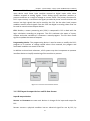
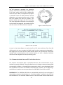
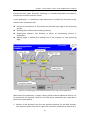
In addition to these basic elements, a PLC system may also incorporate an operator
interface device to simplify monitoring of the machine or process.
Figure 3-1 Structure and elements of PLC
3.1.2 PLC Input & output devices and IO data format
Input & output devices
Sensors and Actuators are two main devices in charge of the input and output for
PLC.
Sensors convert a physical condition into an electrical signal for use by PLC, by
33
Chapter 3 Automation control with PLC&Sinamics Products
connecting to the input modules of a PLC. For example, when a pushbutton connects
to the input of PLC, an electrical signal indicating the condition (open or closed) of
the pushbutton contacts is sent from the pushbutton to the PLC.
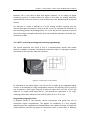
Actuators convert the electrical signal from PLC into a physical condition. Usually
they are connected to the PLC output module. An example is given below to illustrate
that how PLC control a motor starter to provide or prevents power from flowing to
the motor.
Figure 3-2 Motor starter as actuator controlled by PLC
As shown in the figure, the PLC receives signal from a pushbutton, according to the
programs stored inside the memory of PLC, it will update the state of the output
which is to give to the actuator. If the output state is ‘1’, also represents ‘on’, then the
starter will start the motor. Otherwise the motor would be in stop condition.
IO Data format
As for the input and output data format for the PLC, there are two categories:
Discrete and Analog.
Discrete input and output also refer to digital Input and output, from computer
science points of view, digital input and output could be represented by a binary
code: 0 and 1, which stands for 2 states. Therefore, they are usually linked to the
device such as pushbutton, toggle switch and relay contacts, since these devices have
only two possible states: on and off.
So as an example, a lighting system controlled by PLC and the PLC has only digital
input and output. Its input is given by a toggle switch which controls the on and off
of the lamp, the output of PLC is 24 volts voltage given to the lamp. The PLC defines
the controlling logic: when input logic is 1 then output logic would be 1. As
consequence, if we turn the toggle switch on, the lamp will be on.
Analog input and output are able to represent a number of states, or rather, saying
that analog data are continuous, variable signals. Analog inputs are given to the PLC
by analog measuring devices such as thermometer, voltmeter, etc, they give out
34
Chapter 3 Automation control with PLC&Sinamics Products
electric signal whose amplitude could vary continuously.
However PLC is only able to deal with digital numbers, so an analog to digital
converting process is made before the input of the data. An analog would be
represented by a 16 bit or 32 bit or even 64 bit binary code, depending on its defined
format.
For example if a value is defined as a 16 bit analog variable, knowing that the
measuring range of the device is from 0 to 100, so we can calculate the resolution of
this converting process by dividing 100 by 216, in this way we can represent any value
which has integer multiple relationship with the resolution between 0 and 100, by a
16 bit binary code.
3.1.3 PLC’s central processing unit and its programming
The central processor unit (CPU) in PLC is a microprocessor system that makes
decision to update its output, according to instructions held in its program memory,
also based on the memory state and its inputs.
Figure 3-3 Central process unit of PLC
As illustrated in the above figure, the CPU of PLC is made up by integrated logical
circuits. As an example of a logic computation stored in the memory of CPU, the first
row represents a ‘And’ logic, meaning if both the input ‘I0.0’ and ‘I0.1’ are on (be
equal to 1), output Q0.0 would be on. The second row represents a ‘Or’ logic,
meaning output Q0.1 will be on once one of inputs ‘I0.4’ or ‘I0.5’ is on.
Programming language of CPU
A program stored in the memory consist instructions that guide the PLC to
accomplish logical computations. The degree of complexity of a PLC program
depends upon the complexity of the application, the number and type of input and
output devices, and also the types of instructions used. In most cases, 3 different
35
Chapter 3 Automation control with PLC&Sinamics Products
types of programming language are used for PLC, they are ladder logic, function
block diagrams and statement list.
Ladder logic (LAD) is the most popular programming language used with PLC, Ladder
logic incorporates programming functions that are graphically displayed to resemble
symbols used in hard-wired control diagrams.
An example of LAD language has already been displayed in above figure 3-3, LAD
diagrams are read from left to right: The left vertical line of a ladder logic diagram
represents the power or energized conductor. The output coil instruction represents
the neutral or return path of the circuit. The right vertical line, which represents the
return path on a hare-wired control line diagram, is omitted.
Statement list (STL) is a text-based programming language, with this kind of language
people can not only represent basic logic relationship between inputs and outputs,
but also make up some functionality which could not be possible in the LAD language,
one typical example is the recycle of execution programming. In a word, statement
list is the most powerful programming language for PLC, however, in many
applications where only exist simple logics LAD is more preferable due to its intuition.
Function block diagrams (FBD) include rectangular functions with inputs shown on
the left side of the rectangle and outputs shown on the right side. The advantage of
this language is that it has a number of predefined logic structures, it can reduce the
building up time for the functionality in the LAD. However, it is not as intuitive as
LAD.
Following is a figure showing how different programming languages represent the
same logic combination:
Figure 3-4 ‘And’ & ‘Or’ logic represented by different programming language
Programming tools
As mentioned in the basic elements of the PLC, a programming device is necessary
for a PLC. For example, Siemens S7-200 PLC, the programming is done with a
36
Chapter 3 Automation control with PLC&Sinamics Products
computer with the software named STEP 7-Micro/WIN, which is used with the
S7-200 PLC to create a user program.
STEP 7-MicroWIN programming software can be run either off line or online. Off-line
programming allows the user to edit the program and perform a number of
maintenance tasks. When in Offline mode, the PLC does not need to be connected to
the programming device. Online programing requires the PLC to be connected to the
programming device, in this mode, program changes are downloaded to the PLC. In
addition, status of the inputs&output elements can be monitored in the PC.
Excepts STEP 7-MicroWin, there are also STEP 7 Lite special for S7-300 PLC, STEP 7
Professional which consists of the standard tool STEP 7 and the optional packages
S7-GRAPH, S7-SCL, and S7 –PLCSIM.
SIMATIC Manager is the central tool in STEP 7. With SIMATIC Manager, all the “logical”
objects in it represent the “real” objects in the plant system. In SIMATIC Manager, A
Project contains the entire plant system, a Station corresponds to a PLC. A project
can contain several stations that are connected with one another by means of an MPI
subnet, also some IO device interface connected by the sensors and actuators, some
DP slaves such as HMI and PG/PC programming device. In a word, the real structure
of the controlling system could be shown in the SIMATIC Manager correspondingly.
The following figure [fig 3-5] shows the hierarchically tree structure of a SIMATIC
Manager project. The STEP 7 objects are linked with one another through this tree
structure. A project is in the highest level under which followed by the SIMATIC
Station, they could be PLCs connected through MPI, Profibus or Ethernet network.
A SIMATIC station acts as the control Master in its network, in the network other
devices like sensors/actuators, human-machine interface are linked to the station as
slaves. In the Hardware configuration, it is possible to add, take away and arrange
these slave modules, edit their address, etc.
Below SIMATIC station is the CPU folder, under this folder it is possible to modify and
edit the programs stored in the memory of the CPU. All the programs exist under the
Block folder. A block is one assemble of instructions aiming to fulfill a specific task.
For example, the organization block (OB) defines the sequences of calling for other
function blocks or functions. Function blocks and functions are used to fulfill certain
logic computation. Data Blocks (DB) contain the address where variable values are
stored and quoted. UDT block defines a template of data type which eases the
application.
37
Chapter 3 Automation control with PLC&Sinamics Products
Figure 3-5 SIMATIC Manager Project Tree structure
38
Chapter 3 Automation control with PLC&Sinamics Products
Program execution
The PLC program is executed in a repetitive
process, each time of execution is called a scan.
A PLC scan starts with the CPU reading the
status of inputs. Next, the application program
is executed. Then the CPU performs internal
diagnostics and communication tasks. Finally
the CPU updates the status of outputs. This
process repeats as long as the CPU is running.
The time required to complete a scan depends
on the size of the program, the number of I/Os,
and the amount of communication required.
Figure 3-6 PLC Scan process
Figure 3-7 PLC cycle time
As seen in the above figure, the cycle time for a PLC scan could vary from 3 to 100
milliseconds, the more complex the ladder logic (or other programming language) is,
the longer the scan time will be. Other factors which can increase PLC scan times
include serial communications with remote devices, as well as display interfaces
which must be integrated into the processing cycle.
3.1.4 Communication between PLC and other devices
PLC receives and outputs data to peripheral devices, this communication can be
realized by several methods. The most popular one is through a communicating field
connected by Profibus, or through Ethernet protocols which is more developed. Here
the introduction will focus on Profibus communication network, at the beginning I
would like to introduce two concepts about the PROFIBUS DP and AS interface:
PROFIBUS DP: The PROFIBUS DP offers a standardized interface for the exchange of
mainly binary process data between an “interface module” installed in the PLC and
the filed devices. The interface module serves as the DP master and the filed devices
39
Chapter 3 Automation control with PLC&Sinamics Products
serve as the DP slaves. Distributed peripherals are modules which are connected to a
DP master module through the PROFIBUS DP communication network. PROFIBUS DP
is a non-proprietary standardized communication network based on the European
Standard EN 50170 for the connection of standard DP slaves.
Actuator/sensor interface: The actuator/sensor interface (AS interface) is a
networking system for actuators and sensors at the lowest field level. An AS Interface
Master can control up to 31 AS interface slaves through a two-wire AS interface cable.
The cable transmits the control signals and the supply voltage.
PROFIBUS DP master system
The communication between PLC and other devices can be realized by DP master
system. In this network, PLC acts as the DP master, and other devices such as AS
interface act as DP slaves. The DP master communicates with its DP slaves by means
of cyclic data transmission.
This kind of network can comprise maximum of 32 stations, the entire network can
interconnect a maximum of 127 stations. The maximum number of DP slaves in a DP
master system is determined by the type of DP master used. A SIMATIC station can
have several master systems.
Following is an illustration showing the structure of a PROFIBUS DP master system.
DP Master
DP Master:
CPU 318 2DP
Repeater
PROFIBUS DP
DP/AS interface link
PG/PC
SIMATIC HMI
Actuator2
Actuator1
Sensor2
Sensor1
DP Slave
Drawing 3-1 PROFIBUS DP communication system
As shown in the illustration, a PLC’s CPU acts as the DP Master in this network, it
communicates data with sensors and actuators thought a DP/AS interface link
attached to the PROFIBUS DP, besides there is a SIMATIC Humam-Machine Interface
40
Chapter 3 Automation control with PLC&Sinamics Products
for easy monitoring and modification the parameters in the CPU. In the network,
there is also a PG/PC device acts as the programing device for the PLC. Also, by using
a repeater the PROFIBUS cable can be extended to a larger length.
With electrical transmission pursuant to EIA-485, twisted pair cables with
impedances of 150 ohms are used in a PROFIBUS DP. Bit rates from 9.6 kbps to 12
Mbps can be used. The cable length between two repeaters is limited from 100 to
1200 m, depending on the bit rate used.
3.1.5 An example of PLC control system: PLC motor control
After knowing the basic structure and programming language of PLC, now it’s enough
to understand how the PLC works in control system, here is given an example of a
realization of PLC motor control.
In the below figure [fig 3.5] is shown the layout of a simple motor control system,
there are 3 digital inputs and digital 3 output for it, more specifically, a normally open
Start pushbutton is wired to the first input (I0.0), a normally closed Stop pushbutton
is wired to the second input(I0.1), and normally closed overload relay contacts are
connected to the third input(I0.2), these inputs are used to control normally open
contacts in a line of ladder logic programmed into the PLC. As for the output, the first
output point (Q0.0) is wired to the motor starter that initiates the motor when
energized, the other two output points (Q0.1 & Q0.2) are wired to two indicator
lamps indicating the run or stop state of the motor.
Figure 3-8 PLC motor control layout
Initially, I0.1 and I0.2 status bit are on because both the stop button and the overload
stop button are closed, they are similar with the cradle system: when cradle stops
the baby would cry, so keeping the contact on is the sign of safety. I0.0 has remained
41
Chapter 3 Automation control with PLC&Sinamics Products
in logic 0 until the start button is pressed. The logic of Q0.0 depends on the status of
I0.0, I0.1, I0.2 and even itself. Since I0.0 and Q0.0 are 0, so at the scans before I0.0
becomes 1, Q0.0 can only remain at 0. So also Q0.1 and Q0.2 are 0. In network 3,
since Q0.0 logic is 0, then the status of normally closed contacts is on, so Q0.2 is on,
stop indicator is on.
When the Start pushbutton is pressed, the CPU receives a logic 1 from input I0.0.
This causes the I0.0 contact to close. All three inputs are now in logic 1. The CPU
sends a logic 1 to output Q0.0. The motor starter is energized and the motor starts.
Next scan, since Q0.0 is on, the second access to the right now is possible, so even
the pushbutton (I0.0) is released, Q0.0 will remain in logic 1. Meanwhile, Q0.1
becomes logic 1 and in network 2 run indicator is on. Now the motor is running in
the light of run indicator.
When the Stop pushbutton is pressed, input I0.1 turns off, the I0.1 contact opens,
output coil Q0.0 de-energizes, and the motor turns off. When Q0.0 becomes logic 0,
then since in network 3 the status of the normally closed contact is on, so Q0.2 will
become on then the stop indicator on.
Another situation occurs in running condition is that, when overload happens, the OL
contact open and I0.2 logic becomes 0, in network 1 the third contacts’ status
becomes off, then Q0.0 becomes off and the motor stops.
42
Chapter 3 Automation control with PLC&Sinamics Products
3.2 Electric motor controller: Sinamic S120 Drive
In most case of automation of spooling machine, mechanical energy is provided by
two mechanisms: hydraulic system and electric drive. Hydraulic drive has advantage
for providing huge force to move heavy components in the machine such as the
counter knife, while when deal with control of relative smaller component such as
the traverser of spooling machine, an electric motor is preferable.
The control of electric motor base on the elaboration system which regulate the
electrical variables in the motor, with an objective of generating proper supplying
voltage for the actuator according to the reference input variables which could be,
position, velocity, and torque.
For most of converting machine produced by IMS Deltamatic, electric motors control
is realized by the Sinamic products. More specifically, SINAMICS S120 Drive.
Figure 3-9 Motor control with SINAMICS S120
This figure shows that with SINAMICS S120 servo control, we can realize the
close-loop current control and speed control with feedback from the motor, while
position control are complete by higher level controller such SIMOTION and SIMATIC
S7, or just use the Simplified positioning of SINAMICS S120.
3.2.1 Layout of S120 drive system
A S120 drive control system could be divided into 3 levels, the highest level is a
controller such as PLC, giving logic control and setpoint reference. In the second layer
43
Chapter 3 Automation control with PLC&Sinamics Products
there are Control unit and line module, while in the lowest level are the motor
modules and the motor controlled by them, sensors modules.
Figure 3-10 Layout of SINAMIC S120 system
Control unit are the Central control module, the feedforward and feedback control
functions for several Line modules and motor modules are implemented in this
module. For a control unit the following functions are available:
Closed-loop control of the Active Line Module
Closed-loop control for the drive(comprising the motor, Motor module, speed
sensor/position encoder, and Sensor Module)
Communication with a higher-level controller
Communication with the commissioning system(STARTER)
Evaluation of the inputs/outputs on the Control Unit
Evaluation of the optional Terminal Modules
Evaluation of an Option Board plugged into the Control Unit
A line module is a power component that generates the DC link voltage for one or
more motor modules from a 3-phase mains voltage.
In the lowest level there are Motor modules,a motor module is a power unit(DC –
AC inverter) that provides the power supply for the connect motors. A motor module
must be connected to a Control unit via a DRIVE-CLIQ. The open-loop and
closed-loop control functions of the motor module are stored in the control unit.
For the electric motors that can be driven by SINAMICS system, by connecting to the
motor modules via Drive-CLIQ and a power wire. A basic distinction is made between
rotary and linear motors with regard to their direction of motion, and between
synchronous and induction motors with regard to their electromagnetic operating
principle.
As to DRIVE-CLIQ, it is a communication system for connecting the different
44
Chapter 3 Automation control with PLC&Sinamics Products
components of a SINAMICS drive system. The DRIVE-CLIQ hardware is based on the
Industrial Ethernet standard and uses twisted-pair lines. The DRIVE-CLIQ line
provides the transmission and receive signals, as well as the +24V power supply.
Another important component in the layout is the encoder. An encoder is a
measuring system that captures actual values for the speed and position values and
makes them available for electronic processing. Depending on the mechanical
construction, encoders can be integrated in the Motor or mounted on the external
mechanics.
Sensors modules are hardware modules for evaluating speed/position encoder
signals and providing detected actual values as numerical values to the motor
modules via DRIVE-CLIQ.
3.2.2 Control unit speed control process
1. Speed control regulator
Figure 3-11 Velocity feed-back control in Control unit
speed control is realized by a closed-loop control strategy in the control unit for each
drive, as shown in the following figure, the input parameter is the reference speed in
[rpm], after compared with the feedback signal indicating the actual speed which
measured by a encoder mounted on the motor, the difference of speed is inserted
into a PI controller. The parameterization of the regulator is fulfilled through the
inputs value, in particular, it is possible to configure the p gain with a liner mode
according to a reference signal. In the winder or unwinder for example, the p gain is
45
Chapter 3 Automation control with PLC&Sinamics Products
linearized with the diameter of the bobbins since it is required to change with the
mass of the bobbin.
2. Torque compensation and limit
Torque Compensation: The output from the PI regulator is a torque in unit [Nm],
except the torque output from the PI, a torque compensation functionality is made in
order to reduce the effect of friction and inertial in the motor, thus to increase the
precision of the velocity control, and render the system more reactive with the
change of load applied on the motor. Here the control is a feed-forward strategy, the
factor indicating the characteristic of the friction and inertial is input from upper
controller obtained by calculation.
Figure 3-12 Torque compensation for velocity control in Control unit
Torque limit: Torque limit function set limits for the torque reference, this limit can
be calculated as the minimum value between the maximum torque reference input
and the physically limited torque derived from the motor characteristic curve, such
as limit of current or limit of power.
Torque limit is applied to guarantee the motor drive operates in a safety condition
and work continuously without overload or overheating.
46
Chapter 3 Automation control with PLC&Sinamics Products
3. Current control
The torque reference then is converted into current reference which can generate
the required torque. Since the motor to be controlled is an AC motor, the control
current will be 3 current vector components, while they are transformed in two
space-phasors iq and is, obtained by Park transformation, for easy controlling
operation.
Both of these two space-phasors pass the PI regulator and generate two
corresponding voltage references.
Figure 3-13 Current control in Control unit
47
Chapter 3 Automation control with PLC&Sinamics Products
4. Pilotage of phase voltage
Figure 3-14 Pilotage of phase voltages by means of PWM modulation
In the last stage of speed control, two output reference voltages are converted into 3
phase voltage by the PWM technique, these 3 phase voltage then are to be applied
to the AC motor.
3.2.3 Motor control parameter
With S120 drive it is possible to do control like speed, torque and current control,
these controls are realized by a series control parameters stored in the RAM and
ROM of the control unit. There are two kinds of control parameter starts with “p” +
“control parameter number” and “r” + “control parameter number”. “p” means this
control parameter could be modified by inputs from controller in higher level. “r”
means that the parameter are so called “read only” type.
Figure 3-15 Description of control parameter quoted from the manual of S120
48
Chapter 3 Automation control with PLC&Sinamics Products
Here we can see an example of control parameter p1459, it is an control parameter
has a data type of FloatingPoint, that is, a 32 bit data. This control parameter is used
to set the adaptation factor for the P gain of the speed controller.
All the control parameters can be found in the expert list of the motor module from
the software side, as seen in figure 3.13.
Figure 3-16 Expert list in Control unit
This is an expert list for Drive_2, that is the second motor module controlled by
Control unit, we can see in the expert list there are two colors parameters, green
parameters started with ‘p’ so they and adjustable, yellow ones are read only. For
each control parameter there is a text explanation, and for green parameters, in the
value column we can modify the default value for it.
By setting the expert list of the drive, we can realize the assignment of reference
value of speed, torque, or current, for closed-loop control.
49
Chapter 3 Automation control with PLC&Sinamics Products
3.2.4 Communication tools: Telegram
Communication between motor module and control unit is via Drive-CLIQ, while
communication is necessary between control unit and PLC via PROFIBUS DP, this
communications are realized by telegram, a standard or user-define parameter frame
used for communication.
A telegram is a sequence of control words which linked to predefined control
parameters in the expert list. There different standard telegrams aiming at different
functionalities of the drive, such as telegram 1, 2, 102,105 for servo control, telegram
20, 220,352 for vector control. Different telegrams have specific data structure
designed for certain drive functionalities. For example, below is telegram 105:
Table 3-1 Telegram 105 data structure
PZD
1
2
3
4
5
6
7
8
9
10
105 Planned
STW1
NSOLL_B
STW2
M_Red
G1_STW
XERR
KPC
105 Actual
ZSW1
NIST_B
ZSW2
Msg.W
G1_ZSW
e.g.G1_XIST1
e.g.G1_XIST2
Telegram 105 is a very popular one when motor position control is required, it
contains the data in 10 double words, the first word in one double word represents
for the data transfer from the controller to the drive, while the second word
represents for the value transfer from the drive to the controller. That is, in this table,
the first row is the setpoint value for input, the second row is the actual value for
output. The individual data items have the following meaning:
STW
NSOLL
M_Red
XERR
G1_XIST1
G1_XIST2
Control word
Set speed
Torque derating
System deviation(for DSC)
KPC
ZSW
NIST
MeldW
Position controller gain
Status word
Actual speed
Message word
Cyclical actual value (incremental encoder)
Absolute actual value(absolute encoder)
With telegrams, Control unit communicates specific data with upper controller, in
this way upper controller realizes the configuration for control profile, inputing
setpoints or monitoring actual value, and completing some other operations.
50
Chapter 3 Automation control with PLC&Sinamics Products
PROFIBUS DP
Telegr1
Telegr3
Telegr2
Telegr4
Control Unit
Profibus Interface
Exp.list for motor module 1,2,3,4 & CU
RAM&ROM
Drive-CLIQ Interface
Motor
Module 1
Motor
Module 2
Motor
Module 3
Motor
Module 4
Drawing 3-2 Drives communication with telegram
The drawing above shows a complete communication system for Sinamic drive:
1) At the bottom level, motor module communicates with control unit through
Drive-CLIQ, they receive commands from control unit and reports the actual state
parameter of the motor.
2) Inside the Control unit, in the RAM&ROM, there is an expert list for each motor
module connected to the control unit, in the expert list are stored all the
parameter related to a motor drive, adjustable or ready only. Data from
downstream device pass through Drive-CLIQ interface and updates their values
stored in the expert list.
3) At the high level, Control unit is connected into the PROFIBUS-DP network as a
DP slave. Control unit communicates with upper level controller used telegram
defined for each motors, only the particular parameters assembled in the
telegram are communicated. In this way, commands and setpoints from upper
controller pass through Profibus interface and updates their values in the expert
51
Chapter 3 Automation control with PLC&Sinamics Products
list, also upper controller receives the motor actual value by reading the expert
list.
With the realization of this communication, motors can be control by PLC in the way
that gives out speed reference value at the output module address which is linked to
the Control unit input address for the speed setpoint in telegram.
52
Chapter 3 Automation control with PLC&Sinamics Products
3.3 Spooling machine traverser control with SINAMIC
Up to now we have an overview about the control components and architecture for
electric motors. That is, PLC controls the logic and sends setpoints such as reference
speed to SINAMIC drives, SINAMIC drives receive commands and realize the
close-loop control of the motors. In this chapter we will discuss the possibility of
controlling traverser by Sinamics.
3.3.1 SINAMIC traverser control theory
In the case of controlling the traverser in spooling machine, the concept is the same.
There are two key motors realizing the spooling function for the webs: Winder axis
and traverser axis. The former one drives the rotation movement of the winder and
makes the winding function. The second one drives the horizontal movement of the
traverser, guiding the web’s position wound in the winder shaft. Therefore, a
spooling function control is actually a combination of the control for these two axes.
Now I recall the traverser motion profile [fig 2.9] introduced in Chapter 2:
Figure 3-17 Traverser Motion profile
Let’s focus on the displacement profile of the traverser, as the winder axis position
increases, the position of the traverser varies, in the first half period it increases and
decreases in a symmetrical profile in the second half period. So we can say, the
traverser axis is moving synchronously with the winder axis.
So now the key becomes: How to realize the synchronization of movement between
two motor axes.
53
Chapter 3 Automation control with PLC&Sinamics Products
Synchronization can be divided into several types: Position synchronization, speed
synchronization, complicated synchronization.
In position synchronization the slave axis is trying to follow the same trajectory
of the master axis, if difference of position exists at the beginning a correction
would happen to eliminate this gap between two axes. Finally it will reach a
steady state in which two axes would have same displacement and speed.
In speed synchronization the case is simpler, the slave axis would finally have the
same speed as its master, position gap is not considered.
In complicated synchronization, slave axis does not just follow the position or
speed simply, the speed or position setpoints for salves are modified by a
defined function, this function could be time-invariable or varies according to
other inputs.
Obviously, the traverser is synchronized with the winder with a relation function. So,
a complicated synchronization is realized as below:
Speed&Position
setpoints for winder
Relation
function
Speed&Position
setpoints for traverser
Winder Drive
Actual
speed&position
Traverser Drive
Drawing 3-3 Complicated synchronization between two motor axes
As shown in the figure, winder axis and traverser axis are controlled separately by
reference value given by controller, Speed and position reference for the traverser
drive come from the setpoints for winder after the relation function’s modification,
this function is a function depends on the actual speed or position of the winder
drive so a feedback of the actual from the winder drive is necessary.
3.3.2 Traverser control control with PLC&Sinamics strategy based on EPOS function:
In Sinamics drive, position control is not convenient, but as seen in figure 3-9, S120
Simplified position (EPOS) control could be used in the Sinamics. The EPOS setpoint
input mode: MDI, it is a function with reference input from PLC then the drive would
move to the reference position in the reference velocity.
54
Chapter 3 Automation control with PLC&Sinamics Products
Then, an ideal occurs about the spooling traverser control, that is: Updating the
setpoints of position and velocity for the traverser with the calculation of PLC and
then send them to the EPOS function in the Control unit, thus to create a virtual
relation function between the two axes. Since in this control structure only PLC and
Sinamics are involved, so we call it PLC&Sinamics control strategy.
Truly speaking, PLC&Sinamics control strategy is simply and intuitive. In hardware
aspect, the control unit connects to the PROFIBUS network as a DP slave the same as
others slaves, no more modification on hardware configuration is necessary. In
software aspect, since the motor are controlled by sending setpoints from PLC, so
the motor controlling program has no big difference as other program in the PLC for
controlling valves, except the output is an analog data. This structure is very suitable
for control motor axis simple, i.e.:
1) The roller axis in the converting machine, because it works at a constant velocity
during the converting procedure.
2) The winder axis in the converting machine, based on the functionality of a roller,
torque limit control is also required for it, which can be realized by Sinamics.
However, when deal with complicated movement as in the spooling traverser,
Control by only PLC&Sinamics is not able to provide perfect performance due to its
computational limitation and structure drawbacks:
1. Low control frequency
Velocity
Time interval
Ideal velocity profile
50ms
Velocity Setpoint
Actual velocity profile
Max speed error
Ramp-up defined by Sinamic
Time
Drawing 3-4 Speed error due to control interval in Sinamic motor control
In this structure, the PLC updates the reference of the controlled axis at a constant
frequency, that is, with a constant time interval. Since the calculation of the setpoints
55
Chapter 3 Automation control with PLC&Sinamics Products
is combined with other control functions for all the devices controlled by PLC.
Therefore in order not to overload the CPU and not to elongate the other function in
higher control level, the updates of setpoints has relative low priority and is
performed in every 50ms.
As seen in drawing 3-4, the ideal velocity is defined by the velocity cam profile of the
traverser, within the acceleration angle the velocity keeps increasing in a constant
rate. Since PLC gives the traverser axis velocity setpoint in a constant time interval,
after the actual velocity ramped up to the setpoint, it will maintain at that setpoints
and before next setpoint arrives, thus introduce a speed error between the actual
velocity and the ideal reference velocity, it is calculated by:
Speed errorMax ≈
𝜕𝑣_𝑖𝑑𝑒𝑎𝑙
∗ 𝑇𝑖𝑚𝑒_𝐼𝑛𝑡𝑒𝑟𝑣𝑎𝑙
𝜕𝑡
From the formula it is obvious that two factors affect the speed error:
1. Bigger variation of the speed reference, larger speed error. So this is why in the
control of roller axis or winder axis control shows no obvious defects, because
these axes operates with a velocity quite constant. While in the spooling traverser
case, the velocity profile is more complicated, velocity changes in different
segment in one cycle. If PLC&Sinamics control is adopted, big speed error would
happen.
2. Time interval is a determinate factor, since the calculation of setpoints and
update of output for the drive are integrated in the PLC with all the other
program for the whole plant, the control time interval would be elongated due to
the calculation ability of the PLC, and not enough priority of the process, 50ms is
not a short time in motor control, it would introduce speed error can’t be ignored,
thus influence on the spool products quality.
2. Low transmission rate
In this structure Control unit is a DP slave of the PLC, the same as other devices, so
they share the same PROFIBUS network with a 1.5 mbps transmission rate, this
transmission rate is limited by the total transmission length of the network and the
number of DP slaves. Remember that for one motor axes the telegram takes up
about 20 bytes(for telegram 105), so only 75 telegrams can be transferred in one
second without considering other devices. Due to this low transmission rate, a
transmission delay would occur, it takes about 10ms.
In the drawing 3-5 it can be illustrated the effect of the transmission delay, it
introduces a speed reference error, it is the difference between the actual speed
reference and the ideal velocity reference. It appear as the lag of motion in the
motor axis, however this lag phenomenon would be more series in the spooling
traverser since the cam function needs a feedback from the motor to make decision
56
Chapter 3 Automation control with PLC&Sinamics Products
about the speed reference.
Velocity
Transmission delay
Ideal velocity reference
10ms
Actual velocity reference
Speed reference error
Time
Drawing 3-5 Speed error due to transmission delay in Sinamic motor control
3.3.3 Traverser motion profile realized by DCC chart
In Control unit there is a small CPU which is able to deal with simple logic or
numerical computations, it provides the possibility to insert programs to regulate the
control parameters of the drives controlled by it.
DCC (Drive Control Chart) is a type of program aiming at elaborating the control
parameters deriving from drive expert list. As in the traverser case, it could be used
in the Control unit for realizing the modification of setpoints for the traverser axis,
thus to regulate its motion profile.
DCC Chart
Drive
Exp.list
Parameters
Mathematical
Calculation:
Output Direction
∂
+,-,*,/,∂t , 𝑑𝑡
Drawing 3-6 DDC Chart functionality
With DCC chart, it is possible to build up a modification function to edit the setpoints
57
Chapter 3 Automation control with PLC&Sinamics Products
of the traverser according to the feedback parameters from rewinder and settings
transferred from upper controller, following is a standard application provided by
Siemens for Sinamics traverser control.
In this application, it is possible to input parameters to modify the characters of the
traverser axis. Parameters like:
Position A and Position B: They define the left and right edge of the traversing
process.
Winding step: It defines the traversing velocity.
Acceleration distance: The distance in which an accelerating process is
undertaken.
Waiting angle: It defines the waiting time of the traverser at each traversing
edge.
Figure 3-18 Settings page in the Standard Sinamics traversing control application
With these five parameters, a simply velocity profile without additional velocity can
be created for the traverser. Now let’s see how these parameters are converted to
the actual motion profile:
1. Position A and Position B are the two position setpoints for the MDI function.
First traverse moves from left to right with a position reference of position B, it
58
Chapter 3 Automation control with PLC&Sinamics Products
stops for a while after on its arrival at Position B. A changeover switch is activated
when the it received a ‘waiting angle reached’ signal, then the setpoint of
position change from B to A, the traverser starts to move from right to left.
2. The waiting angle is the rotational angle winder makes in the time interval the
traverser stops. It is realized by integrating the winder velocity over time,
meaning that with the input of waiting angle value from the PLC, in DCC chart it
will check if the integration of winder velocity over time reaches this setting value,
to send out the ‘waiting angle reached’ signal.
3. Winding step is realized by using the velocity override according to the input of
rewinder velocity. Override means the percentage of the reference value.
Velocity overrides is quantity referred to the setpoint in expert list parameter
p2691. Here winding step is the traversing length in one rewinder cycle, so:
v=
winding_step ∙ winder_velocity
2𝜋
We can obtain the required velocity to realize the winding step.
4. The acceleration distance is implemented using the acceleration and deceleration
override, they are quantities referred to parameters p2572 and p2573. Here, as
the acceleration distance is known, according to formula:
a=
a: Acceleration
𝑣2
2𝑠
v: Constant Velocity
s: Acceleration distance
We can obtain the required acceleration for acceleration distance.
Drawbacks and Disadvantages:
1. Error caused by reaching override limits
The application calculates the acceleration and velocity of the traversing arm as
override, it can be a maximum of 100% for acceleration and 200% of the
reference parameter. It would occur that the required acceleration or velocity is
over than 200% of the reference, in this situation the acceleration or velocity
control introduces errors.
2. Hot parameterization causes problems
It doesn’t support hot parameterization. If user wants to change the settings, it is
required to first power-down the traversing axis. Because the application must
59
Chapter 3 Automation control with PLC&Sinamics Products
first accept the new values and must adapt the override. Otherwise, it can occur
that the traversing arm will accelerate at an unexpectedly high level or will move
at a high velocity. With the change parameterization, it would also happen that
the mechanical load capability of the traversing arm will be exceeded.
3. Position Error caused by velocity profile digital control
The traverser motion is controlled by regulate its velocity profile, in digital control
the velocity function is discontinuous so the position would result in unavoidable
error if it is obtained by integration. For example, as introduce before, the waiting
angle is obtained by integrating the actual velocity of the rewinder. Since the
actual velocity fluctuates all the time, the sampling frequency affects a lot the
precision. Due to this reason, integration of speed could always deviate from the
real value, a better way is to control the position profile directly, not through the
speed profile.
4. Limited computational ability of CPU in CU
In Control unit the CPU doesn’t have a strong computational ability, as introduced
before, each CU can control only 4 to 6 motor modules according to theirs types.
So if the DCC chart programs are too complicated, it could occupy the
computational space of the CU and therefore reduce the number of motor
module it can control. Based on this information, with DCC chart it is hard to
create a complicated velocity profile. For example in the standard application, the
traverser velocity profile is simplified, taking away the additional velocity
segment.
5. Language Limited
Compared to high level test based programing, DCC chart language is not so
efficiency in creating complex mathematical equations, this is also a limit for
generating complicated complex velocity profile.
6. Diagnostic difficulty
In this application the control parameters are subject to an internal elaboration,
so the user is hardly able to check the state of those parameters when an error
happens, this render the diagnostic difficult.
60
Chapter 4 Simotion controller and tis potential in traverser control
Chapter 4 Simotion controller and its
potential in traverser control
Simotion is Siemens’ flagship motion control platform, a scalable high performance
hardware and software system designed to control the automated movements of a
wide variety of machines.
In software aspect, Simotion controllers are all programmed using Siemens SCOUT, a
software package which is IEC 61131-3 compliant and supports a variety of
programming languages including Ladder, Structured Text, and Motion Control Charts.
It allows central or distributed machine concepts to be realized as well as PC,
controller and drive-based solutions, and also includes tolls for testing,
commissioning and diagnostics.
In hardware aspect, Simotion controller comes in three different hardware packages:
Simotion C, P and D. The modular Simotion C is the most general and flexible
platform, while Simotion P is a PC-based controller suited for the most demanding
motion control applications, and Simotion D is a compact, bookcase style platform.
Communications between the controller and drives is done through PROFINET,
PROFIBUS or Ethernet.
Since Simotion is a control tool dedicated for motion control, it could be adopted for
the spooling traverser for the following advantages:
1. High control frequency due to high execution speed benefits from its powerful
integrated CPU.
2. High transmission rate between controller and drives, due to a Profibus network
dedicated for the motor drives.
3. Easy programming for drive due to the introduction of Technological Object
concept, and further application of OOP (Object Oriented Programming), this
brings the possibility of cooperation between multi axes. Besides, Siemens has
developed different kinds of standard program which has a specific functionality
for variety motion task for its client, which simplifies a lot the development of
Motion program and reduces remarkably the development cycle.
4.1 SiMotion hardware layout
Simotion controller is mainly composed by a CPU and an integrated Sinamics drive
which is actually a Control unit. The integrated Control unit is connected to
61
Chapter 4 Simotion controller and tis potential in traverser control
Simotion’s CPU via a Profibus integrated, beside the CPU has several more interfaces
for the connection of PROFIBUS or PROFINET even for Ethernet. As shown in the
following figure, another SINAMICS Drive is connected to CPU through a
Sub-PROFIBUS 2, while Simotion controller connects to the PLC as a DP slave through
the Profibus 1.
The CPU of the Simotion executes specially the programs dedicated for the motion of
motor axes, it works without the burdens come from logic control as the PLC suffers,
therefore it is able to finish a calculation cycle in a very short time.
In the Sub-Profibus network, Simotion is the master and all the salves are Sinamics
drives, so in this Profibus only the data about drive motion are transferred,
furthermore, due to the number of salves decreases and the total transmission
length decreases, the higher transmission rate can be obtained in the Sub-Profibus
network, for example, 12 mbps. As to the communication between PLC and SiMotion,
it contains no more information than the key commands and important setpoints for
the motor axes.
PROFIBUS DP 1
1.5 mbps
SiMotion
DP1
SINAMICS Drive
INTEGRATED
CPU
DP2
SINAMICS Drive
DP3
Profibus integrated
12 mbps
PROFIBUS DP 2
Drawing 4-1 SiMotion hardware layout
Therefore, from the hardware configuration, SiMotion is able to:
1. Separate the calculation of motion control from PLC, releases the PLC workload,
while SiMotion CPU dedicates in motion control with high control frequency.
2. Separate the communication system for motor control from the Profibus for the
whole machine, releases the main Profibus, while for Drives the transmission rate
is improved.
62
Chapter 4 Simotion controller and tis potential in traverser control
3. With its powerful and motion dedicated CPU it is possible to realize variety and
stronger functionalities for more motor axes.
63
Chapter 4 Simotion controller and tis potential in traverser control
4.2 SiMotion software layout
The following figure shows the layout of SiMotion control in software points of view,
it is composed by three parts: User program, TO instance, Execution system.
Generally speaking, user program governs the rule of modification of the technology
object parameters, which is an assembly of controlling parameters. Programs are run
in the execution system.
Figure 4-1 SiMotion software control layout
4.2.1 Technological objects
In SiMotion software system, program is implemented in an object-oriented manner,
this is to treat the motor to be controlled as an object, this object, is an assembly of
all the characteristics of this motor. In this way, each term included in the object can
be modified by the program.
Technological objects are created in SiMotion, they represent for each motor drive
controller in the SiMotion. Remember the control parameters exist in the expert list
64
Chapter 4 Simotion controller and tis potential in traverser control
of the Control unit, Technological object for a motor is an assembly of most
important control parameters in the expert list. This connection between the TO and
control parameters is realized by telegram.
CU
SiMotion
Programs
Telegr
Expert List
Parameters
Technological Object
Drawing 4-2 Technological Object link with Expert list by telegram
In SiMotion, according to different application, 4 types of technological objects axis
are predefined, they are:
1. Velocity axis
This axis is used when the position of the axis is not in the control purpose, the
only value to be regulated is the velocity of the axis. With this type of TO axis it is
possible to realize: Speed control with reference input; Motor control with torque
limit.
2. Position axis
This axis is used when position control is required for the axis. The input for
position can be in two types: relative position or absolute position. With the
position axis it is also able to realize the velocity axis, resulting at the functionality
that: the motor moves to the reference position with a reference speed.
3. Synchronous axis
This axis is used to receive reference value from a master axis, then it becomes
synchronized with the master. Cam function can be applied between two
synchronized axis.
4. Vector axis
A vector axis is able to realize all the functionality of other three types.
Each motor axis controlled by SiMotion is defined as an instance of the 4 types of
technological object, an instance of a technological has all the structure and
characteristic of this object, just like the copy of it. For example, motor_axis_1 and
motor_axis_2 are both the instance of velocity axis, they have both the accessory
parameter
‘actual_velocity’,
then
motor_axis_1.actual_velocity
and
motor_axis_2.actual_velocity stand for the actual velocity for each axis.
After the motor axis instances are defined, the linkages between instances and
corresponding expert list are built. Modification about the instances accessory
parameters means directly modification to the expert list. Therefore, SiMotion
programs is able to control the parameters of the drives.
65
Chapter 4 Simotion controller and tis potential in traverser control
Commons: With the application of technology object, the synchronization control
between two axes becomes easier. This is very fit for the spooling traverser case,
where complicated synchronization is needed between the winder axis and the
traverser axis.
4.2.2 Program unit
The programs of SiMotion appear as program unit, it is a paragraph of code written
in one of the three program language: Ladder, Statement text, Motion Control Charts.
Among them statement text is the most used one due to its versatility, however
ladder and MCC have their advantage of intuitive.
Here I will focus on the description of Statement list since most of the user program
and library program are written in this language. It is a language at high level
compliant to IEC 61131-3, it favor the elaboration of data and calculus mathematical,
guaranteeing high degree of freedom for programming.
A ST unit is composed by two sections: Interface and Implementation:
INTERFACE
USES Declare technological package, libraries, Units to use
VAR_GLOBAL (RETAIN) / TYPE
Declare variables and types of variables
END_VAR
Declare programs, Functions, and Function Block
END_INTERFACE
IMPLEMENTATION
PROGRAM
VAR (RETAIN) / TYPE
Declare local variables and types of local variables
END_VAR
Instructions
END_PROGRAM
END_IMPLEMENTATION
In the ‘Interface’ section, it is first declared the TO package libraries and some
defined units, in this way the variable symbol or function defined in the used units
are available in this unit. Then the global variables which can be used not only in this
unit but also in others are defined. At last are defined the programs to be run in this
unit, also the function or function block to be used.
The difference between functions, function block and programs:
66
Chapter 4 Simotion controller and tis potential in traverser control
Function has input variables and it returns a value, the local variables during
process dismiss after the function ends.
Function block has input variables and output variables, all the local variables are
stored in the memory and recall after the function block ends.
Program has no input nor output variable, it elaborate instructions and stored
the local variables.
In the implementation section, first local variables are defined, this include the
declaration of instance for function or function block. Then the instructions describe
a specific way to elaborate with the variables, these way including mathematical
calculations, logic judgment etc.
Commons: The program unit brings the concept of function block, which is very
suitable to be applied for the cam function of the spooling traverser. With the
function block, a cam functional could have some inputs, these inputs can be
parameters to modify the cam profile, such as acceleration angle, total angle,
additional velocity in the traverser motion profile. With the inputs the function block
generates a series output, they are the polynomial factors for each segment of the
traverser motion profile, thus to define the cam profile.
4.2.3 Execution system
All programs are executed in the SIMOTION device execution system, which provides
a series of execution levels with various execution properties. Programs must
therefore be assigned to the execution levels in order to be executed.
Figure 4-2 SiMotion execution system task level
67
Chapter 4 Simotion controller and tis potential in traverser control
In this figure we can see several task levels, each of them occupies a certain length of
time. Tasks are called in sequence according to their priority. For example,
communication DP task has the highest priority so it is executed first, then is
executed the task servo and task IPO, interrupt task and Round-robin.
An important thing is that each task level has their cycle clock:
Clock DP: The bus cycle clock is based on the cycle of the isochronous bus and
determines the time intervals for data exchange with the DP/PN I/O. The bus
cycle clock is used as the basis for setting further cycle clocks.
Servo cycle clock: The servo cycle clock can be set as a multiple of the bus cycle
clock but a cycle clock ratio of 1:1 is recommended. Among other things,
position control and monitoring of axes, drive communication, and I/O
processing take place during the time slice of the servo cycle clock. The cycle for
the servo cycle clock determines the interval between two position control cycle
clocks.
IPO cycle clock: A cycle clock ratio of 1:1 is recommended. This is a time slice of
the interpolator cycle clock is used, amongst other things, to calculate the
setpoints. The cycle for the interpolator cycle clock determines the interval
between two interpolator cycle clocks. Time slice requirements may increase
briefly at the start of one or more commands.
IPO2 cycle clock 2: Interpolator cycle clock 2handles the same tasks as the
interpolator cycle clock and can be used for technology objects of lower priority
classes. The IPO2 cycle clock can be set as a multiple of the IPO cycle clock.
As shown in the figure, here IPO cycle clock is twice of the Clock DP, if the
communication task is executed every 3 ms, then in task IPO level the task is
executed in every 6 ms.
System tasks are executed in the high execution level, just like task in charge of
communication or interpolation. Besides them, there are the user tasks. They are
programs made by user to realize certain motion or control purpose, usually in lower
execution level than the system task.
There are 5 user program tasks: Startup task, synchronous tasks, timer interrupt tasks,
motion tasks and background tasks.
Startup task is provided for the one-time initialization and the resetting of the
technology objects. It is activated when the operating mode switches from STOP or
STOPU to RUN.
Motion tasks and Background tasks are executed in Round-Robin task level. In this
level, computing time that is not consumed by higher priority tasks is distributed
over the remaining tasks in the round robin principle, meaning that these tasks run
68
Chapter 4 Simotion controller and tis potential in traverser control
one after the other. The next task is always started when the previous task gives up
the computing time (task completed or in the ‘waiting’ state). The computing time of
a round robin task is limited to the maximum number of servo task, however the
system ensures that a round robin task always gets at least the computing time of a
servo cycle clock.
In this segment of time, user programs are divided into two types:
1) Motion tasks: They are intended for the programming of sequences, for
programmed motion control or other sequential executions. For example, an axis
traverses to a target position, waits for an enable signal, and then traverses to the
next target position.
2) Background tasks: They are the programs of cyclic sequences without a fixed time
frame. They are executed cyclically in the round robin execution level, which
means it will be automatically restarted on completion. Usually background tasks
are used to implement cyclical logic functions, interlocks, calculations and
monitoring functions.
Commons: From the description of the SiMotion execution system we can discover
its largest advantage for the application of spooling machine, since the interpolator
function is executed in IPO task level, meaning that the update of setpoints could be
realized in every IPO cycle clock, it is a very short time respecting to the cyclic time of
PLC. Therefore, a high control frequency could be obtained.
69
Chapter 4 Simotion controller and tis potential in traverser control
4.3 Simotion traverser control concept
Simotion’s OPP programing broadens the concepts about traverser control, firstly,
position control and axes synchronization can be easily realized by the technological
objects. More importantly, in Simotion between synchronous axes cam profile can be
inserted.
Virtual cam function
A virtual cam profile has the same concept as the real cam, a real cam transforms
rotational movement to linear movement, or more fundamentally, a cam transforms
one motion profile to another. From mathematical point of view, this effect could be
express by a cam function.
In the spooling function, Cam function are defined as a piecewise function which
contains 16 segments, each segments in the function represents for each period in
the traversing cycle:
Segment 1: Acceleration angle 1
Segment 2: Velocity Spike 1
Segment 3: Transient from spike to FCA
Segment 4: FCA (Forward constant angle)
Segment 5: Transient from FCA to spike
Segment 6: Velocity Spike 2
Segment 7: Acceleration angle 2
Segment 8: Waiting angle 1
Segment 9: Acceleration angle 3
Segment 10: Velocity Spike 3
Segment 11: Transient from spike to BCA
Segment 12: BCA (Backward constant angle)
Segment 13: Transient from BCA to spike
Segment 14: Velocity Spike 4
Segment 15: Acceleration angle 4
Segment 16: Waiting angle 2
In the cam function, each segment can be expressed in a polynomial function with
the highest power of 6, thus to simulate the cam curve in each segment. So for each
segment, it is defined with 7 factors for each polynomial terms and 4 parameters for
the boundary coordinates.
From this concepts, we can define the Cam function for traverser:
𝑎0,1 + 𝑎1,1 ∗ 𝑦 + 𝑎2,1 ∗ 𝑦 2 + 𝑎3,1 ∗ 𝑦 3 + ⋯ + 𝑎6,1 ∗ 𝑦 6 (0 ≤ 𝑦 < 𝐴𝐴1)
𝑎0,2 + 𝑎1,2 ∗ 𝑦 + 𝑎2,2 ∗ 𝑦 2 + 𝑎3,2 ∗ 𝑦 3 + ⋯ + 𝑎6,2 ∗ 𝑦 6 (𝐴𝐴1 ≤ 𝑦 < +𝐴𝑆1𝐶)
…
f(y) =
…
…
2
𝑎
+
𝑎
∗
𝑦
+
𝑎
∗
𝑦
+
⋯
+
𝑎6,16 ∗ 𝑦 6
(𝑇𝐴 − 𝑊𝐴 ≤ 𝑦 ≤ 𝑇𝐴)
{ 0,16
1,16
2,16
an,m
: Polynomial factors, n is the number of terms, m is the number of segments
AA1
: Acceleration angle in the traverser motion profile
+AS1C : Acceleration angle + Spike length 1
70
Chapter 4 Simotion controller and tis potential in traverser control
TA : Total angle in one traversing cycle
WA : Waiting angle in the traverser motion profile
In this function f(y) stands for the displacement of the traverser, it is a function of the
y, which stands for the displacement of the winder in degree. Since the movement of
the traverser is cyclical, this function stands only for one cycle movement. When next
traversing cycle starts, y value starts from 0 again.
Synchronization between rewinder and traverser
As shown in the following figure, rewinder drive is defined as a position axis in
Simotion, as the master of traverser axis, it should provide the position reference to
its synchronous axis.
A cam profile is also an object in Simotion, this object contains all of the parameters
that could describe the cam function. Parameterization could be realized by using the
function block, which receives parameters from user and generates the function: A
set of polynomial factors and boundary coordinates.
TO
TO
Position
axis:
Rewinder
Vref,Sref
Cam
profile
function
Synchronization
Synchrono
us axis:
Traverser
Vref,Sref
Drawing 4-3 Traverser axes synchronization through cam
In To it is possible to configure the velocity or position setpoint for axes, also their
actual velocity and position are present. So in traverser axis, the position setpoint is
given by the value derived from the rewinder after cam function calculation. In this
way, traverser will follow the rewinder movement according to a virtual cam profile.
71
Chapter 5 Traverser control by Simotion
Chapter 5 Traverser control by Simotion
From the last chapter we know that Simotion has the ability to separate the logic
control and motion control in the PLC, separate the communication network for all
the motor axes, as a result the control frequency and transmission rate are improved.
These two improvements are able to reduce remarkably the motion error of the
traverser according to the analysis, therefore SiMotion is more suitable to apply for
the traverser motion control.
A project is made to simulate the SiMotion control performance, this project is
completed on a simulation machine composed by all the devices required to
complete a traverser control, such as PLC, Sinamics drives, SiMotion controller, HMI
touch panel, etc.
Project purpose:
1. Buildup a traverser motion control system based on SiMotion for spooling
machine, both the hardware structure and the software programs. With which an
improved performance could be foreseen.
2. With the new system, users have convenient access to configuration of the
characteristics of traverser motion curve, to realize different spooling
approaches.
5.1 Hardware configuration of the Simulation machine
Figure 5-1 Overview of the Simulation machine
72
Chapter 5 Traverser control by Simotion
The figure above shows the overview of the simulation machine, this simulation
machine is made up by 4 parts:
1. PLC Controller: A Siemens PLC SIMATIC S7-300 controller combined with the
Digital Input and output module. (Fig.5.1 Right-Down)
2. Motor controller group: A SiMotion D435 controller, A Sinamics S120 drive with
one Control unit, one Line module and two motor modules. (Fig.5.1 Left-Up)
3. Two Siemens electric motors, on which is mounted a rotating disk. (Fig.5.1
Left-Down)
4. One HMI touch panel in charge of the input and monitor of parameters. (Fig.5.1
Right-Up)
Figure 5-2 Hardware configuration of the Simulation machine
In the figure we can see there are two main Profibus DP networks:
The lower one in the figure connects the CPU of PLC, the CPU of SiMotion
Controller, the HMI and the PG/PC device together. In this network, PLC is the DP
master, all the other devices act as DP master. Transmission velocity for this
network is 1.5 mbps.
DP Master recognizes DP slaves interface by their own defined physical address,
here the address for Simotion controller is 2, for HMI is 20, for PG/PC is 21. The
PLC itself has an address of 3.
The upper one connect Simotion controller and a S120 Control unit, this sub
network has a high transmission rate of 12mbps, as introduced before, it is
special for the electric motor drives. Inside the Simotion controller, there is also
a Profibus integrated connects the Control unit integrated to Simotion’s CPU.
73
Chapter 5 Traverser control by Simotion
PLC’ rack configuration
Figure 5-3 PLC rack configuration
Physically, PLC controller is fixed on a rack with other modules. As shown in this
figure, the CPU of PLC is type 317-2 DP, it is the DP master of Profibus(1), which is
connected the Simotion controller D435. On the rack there are mounted two IO
modules, for input it is a digital input module with direct current at 24 volt, while for
output it is a digital output module with direct current at 24 volt and 0.5 A.
Configuration of Connection between PLC and Simotion
Figure 5-4 Configuration of the connection between PLC and Simotion controller
Communication between PLC and Simotion are through Profibus, it is necessary to
define the docking relation between their peripheral IO address. As shown in the
74
Chapter 5 Traverser control by Simotion
figure, in the configuration window 3rd column indicates the DP address of the
Partner for Simotion, that is the master of Simotion, as we know before, 3 is the
address for PLC, so here Partner address A90 means the output address of the PLC,
its length is a word, it is connected to the input address E9016 in the Simotion side.
This rule goes for the other IO address. In this way the communication is built
between PLC’s CPU and Simotion controller.
Motor drive configuration
Figure 5-5 Motor drive configuration summary
In SiMotion scout, the program used to manage the Simotion controller and its salves,
the drive configuration is made. In this summary we notice three important setting:
1. Control type: Sinamics can realize velocity control in two ways: with encoder or
without encoder. If without encoder, the speed control is made by using the
natural current feedback. While here we have both two motors with encoder, so
speed control is by using the feedback signal from encoder.
2. Motor type: If the motor is connected to the motor module via Drive-CLIQ, then
the information about encoder and other motor characteristic can be transferred
to the controller automatically without necessity to insert them.
3. Process data exchange, Profibus drive message frame type: here we use Siemens
standard telegram 105 for both of the motors, since telegram 105 is aimed at
position control. Since the winder axis and traverser axis are to be synchronized
via displacement, so position control is necessary.
75
Chapter 5 Traverser control by Simotion
Configuration of connection between Telegram and expert list
Figure 5-6 Configuration connection between telegram and expert list
The connection between Telegram and expert list can be edited here, since here we
use standard telegram so the majority of parameters are fixed. If a user defined
telegram is used, it is possible to link the parameter required by the telegram to the
parameter in the expert list here.
76
Chapter 5 Traverser control by Simotion
5.2 Software configuration
5.2.1 Axis configuration
In this spooling simulation project, two axes are required, so in SiMotion scout we
need to first create two axes, one for rewinder and the other for traverser, then
configure them.
Figure 5-7 Rewinder TO axis configuration
Rewinder axis is defined as a position axis, with an IPO cycle clock for interpolation in
position control, axis type is rotary electrical axis. This axis is linked to the rewinder
controlling drive, with an absolute encoder.
Besides the above basic settings, we can also configure the axis data and units of the
axis, etc.
Figure 5-8 Axes synchronization configuration
77
Chapter 5 Traverser control by Simotion
Since traverser axis is defined as a following axis, beside the axis configuration the
synchronous operation should also be configured. Here we can chose which axis the
following axis is linked to, and the cam function between the two synchronized axes.
In the figure we can see from the configuration that traverser axis is synchronized
with rewinder axis, interconnecting through cams ‘Trav01CamA’ and ‘Trav01CamB’,
which are defined in the cam folder.
5.2.2 PLC program block
In the project, since the aim is to test the functionality of the traverser controlled by
Simotion, so the PLC controls only the motion of two motor axes and their
communication between PLC and Simotion, other control functionalities such as web
tension control, bobbin diameter control and safety control are not taken into
consideration in the building of system programs.
Programs in PLC appear in the format of blocks, the program system is made up by
the following blocks:
OB1: Organization Block 1 to arrange the execution of all program blocks in this
project. Here in this block FC1 and FC60 are called.
FC1: Function Block 1, takes control for the power switch of the line module and
emergency input. The logic is that:
With the emergency switch is on, line module power is on when the
corresponding button is pressed for over 2 seconds. When line module power is
on, if the emergency switch is off, then the line module is power off immediately.
FC60: Function Block 60, takes over the communication between Simotion and
PLC, here two sub-function FC630 and FC631 are called.
FC630: Function Block 630 is in charge of the parameter communication for
motor axes, corresponding to the parameters in data structure of velocity axis
and position axis.
FC631: Function Block 631 is in charge of the parameter communication for
control unit, corresponding to the parameters in data structure of ST_Main.
DB2: Data block derived from UDT630, it contains all the parameters to be
communicated for rewinder axis.
DB3: Data block derived from UDT630, it contains all the parameters to be
communicated for traverser axis.
DB600: Data block contains all the parameters to be communicated for Control
unit.
UDT630: User defined type block, it is the standard type for the data block used
for position axis communication, all the other data block derives from here will
have the same data structure, but with different memory address.
78
Chapter 5 Traverser control by Simotion
5.2.3 Simotion Program Units overview:
In the program folder there are 9 ST units and 2 MCC units for completing this
project.
1. ST Units:
ST_Main:
In this unit two programs are present, Background_Main and Ipo_Main, their
execution level can be known from their names. In Background_Main are made the
commands and calculation for the global control purpose, that is, not related to a
specific axis, but particularly for the control unit. In Ipo_Main, following task are
executed:
a. Calculate the web thickness which is used in the function block dedicated for velocity
ramp-up profile generation.
b. Choose the drive from which the parameters to generate the ramp-up are obtained.
c. Call the instance of FB_Ramp_Management
d. Assign the reference speed to virtual matster
ST_Profibus:
This unit is in charge of the communication between Simotion and other device
through Profibus. Six data structures are defined here, they are:
Velocity_Command_Data_struct
Velocity_Status_data_struct
Position_Command_Data_struct
Position_Status_data_struct
Main_Command_Data_struct
Main_Status_data_struct.
Command structure and status structure indicate two data transmission directions:
In the command structure, all the variables have the direction from outwards to
inwards, i.e. they are the input parameters for Simotion programs from other device
connected via Profibus; On the contrary the status structure combines all the actual
values to be output to other devices.
Velocity, Position and Main indicate different data structures for the 3 technological
79
Chapter 5 Traverser control by Simotion
objects: They refer to the technology object axis to which the structure parameters
are linked in Simotion. For example, in velocity structure, the variables contained
inside are those parameters with which can be used to control a velocity axis.
Position structure is for position axis, main structure contains parameters for control
unit.
ST_Global_Types:
In this unit, all the data structure types which could be quoted by other program
units are defined. In fact this unit is an extraction of all the other units’ type
declaration part. In this way the units are clearer and simplified.
ST_Global_Var:
In this unit, all the variables which could be used by other program units are defined.
In fact this unit is an extraction of all the other units’ global variable declaration part.
In this way the units are clearer and simplified.
ST_Rewinder:
The Rewinder axis control unit, this unit is in charge of all the motion control of the
rewinder.
ST_Traversaxis:
The traverser axis control unit, this unit is in charge of all the motion control of the
rewinder.
ST_Trav_Traversaxis:
This unit controls the traverser synchronization characteristic, that is, the cam profile
function. More clearly, it defines the cam profile according to user settings, it take
over the validation of the corrective of the settings and it controls the timing to load
the calculated cam profile to the cam linked between two axes.
ST_Fault:
This unit takes over the fault detective task.
2. MCC units:
MCC_Axis_Management:
It is the pre-control unit for FBlineaxis, the library unit for axis control.
MCC_Axis_Management elaborates the data structure received from PLC and
converts it into the standard input form for FBlineAxis unit. More specifically,
according to the ‘command-byte’ from PLC, it creates an internal module for the
FBline to configure the basic control parameters and make realization of the defined
mode. In this unit 3 function blocks are defined according to their different control
aims in converting machine, they are:
1. Roller Management
For the control of roller, it required only velocity control, in MCC only 3 internal
80
Chapter 5 Traverser control by Simotion
modes are defined: Run, Jog, Stop.
The mode is chosen according to the command byte, when it is equal to:
0: Stop mode: The motor decrease its speed to 0 with a set deceleration, then
disenable.
1: Run mode: The motor is energized and run with the predefined speed.
8: Jog mode: The motor is enabled and can move at the reference speed written
through touch panel.
2. Positioner Management
Operation mode according to command byte:
0: Stop mode: Stop the motor then disenable
1: Absolute positioning slow: Move to the absolute position with set low speed
2: Absolute positioning fast: Move to the absolute position with set high speed
4: Homing: Move to the home position
8: Jog forward: Motor moves forward at speed setpoint from touch panel.
16:Jog backward : Motor moves backward at speed setpoint from touch panel
32: Positioning relative: Move to the set relative position
64: Gearing positioning: Follow the movement of the master axis with a virtual
cam
128: Stop without disenable the motor
3. Winder Management
Operation mode according to command byte:
0: Stop mode: Stop the motor
1: Run mode: Motor follows the line master performing the tension control
8: Jog forward: Motor moves forward at speed setpoint from touch panel
16: Jog Backward: Motor moves backward at speed setpoint from touch panel
32: Shaft homing: Sequence of jog and stop control, first the motor moves in jog
speed until the shaft_homing_signal is received, then it performs a stop at set
deceleration.
FBlineAxis:
FBlineAxis is a standard unit provided by Siemens for the motor movement control.
Therefore it is a unit without any user modification and fit for all the axis application.
81
Chapter 5 Traverser control by Simotion
It is the unit on the lowest level of the TO axis control, it is able to modify the TO
parameters directly according to inputs. It can perform the following task:
Enable/disenable axis
Control the brake integrated in motor
Command the manual operation mode: jog positive or negative, also positioning.
Activation of homing function
Command the automatic operation mode, axis moves with:
Gearing, with relationship fix or variable
Gearing with predetermined Cam profile
External control, for the axis controlled by external functions, like
FB_Winder
Manage the technical alarms of axis.
FbLineAxis
DriveStatus Bool
Bool DriveOn
InSync Bool
Bool StartStop
PhaseDetected Bool
Bool StopMode
InPhase Bool
Bool JogPos
Run Bool
Bool FixedEndStop
ClampingState Bool
Bool OpenBrake
Status
Commands
Operation Bool
Bool JogNeg
Homed Bool
Done Bool
Bool EnablePhaseSynchronisation
Error Bool
Bool ChangeShiftPositionPositive
Bool ChangeShiftPositionNegative
FirstErrorNumber DInt
ErrorObjId Int
Bool AckError
EnumOpMode OpMode
1) No Mode
2) Manual
3) Pos
4) Homing
5) Auto
StructAxisData
StructTechFaultData
sAxisData
sTechFaultData
StructAxisData
StructTechFaultData
Drawing 5-1 FBLineAxis Block IO overview
The inputs for this FB are composed by commands and setpoints. Commands like
Driveon, startstop and JogPos, they are the output of MCC_axis_Management,
Setpoints are contained inside the structure sAxisData, in this structure, there
are also sub-structrue for coordination, for axis configuration, for setpoints, for
actual value and for diagnostic.
Output of this FB are the status parameters and also structure for axis data. The
status parameters are indicators refer to the state of motor axis, in the output
82
Chapter 5 Traverser control by Simotion
sAxisData, there are the actual value of parameters like the velocity and position.
sAxisData is the input also the output, because it is the In&out variable for
FBlineaxis. It passes through the FB, inside the FB part of its parameters are the
input for FB, such as its sub-structure for setpoints which contains the setpoints
like reference velocity and position; parts of its parameters are the output of the
FB, such as its sub-structure for actual value which contains the variable to be
written the actual value by FB; parts of its parameters are the process variable,
such as the TO axis for motor, as introduce before TO axis contains the
parameters linked to the expert list of the drive, these TO parameters are
modified in the FB during the process, by this way, FBlineaxis realizes the control
of motor axis.
83
Chapter 5 Traverser control by Simotion
5.3 Simotion core program unit
5.3.1 Axis motion control program unit
ST_Rewinder and ST_Traverser are the two units for the motor control in my project.
Although rewinder and traverser have different axis type, their control units have
almost the same structure.
Program unit Structure:
As it is a ST unit, it can be basically divided into two parts: Interface and
Implementation.
Interface
In interface except declare the package or units to quote, the definition of global
variable and global retain variable is made.
For global variable, there are 5 variable structures:
Gsctrl_Fbline_XXXX and GsStatus_Fbline_XXXX are two structures for the control
parameters and status parameters.
FB_Line_XXXX is the instance of FBLineAxis, the concept of instant is introduced
before.
FB_XXXX_management is the instance of fb_position_management, this setting goes
for both the rewinder and traverser axis.
Also XXXX_getfaults_sinamics, it is an instance of the get fault function block.
For global retain variable, the parameters defined here have the ability to retain their
value after power-off, they are stored in the ROM of Simotion for easy recall. These
parameters are usually the default settings for the process. Here it is defined a data
structure named gsAxisData_XXXX, this data structure contains the configuration
data, setpoints data for the TO axis to be control.
Ps: Here XXXX represents for the name of the axis.
Implementation
Implementation part is composed by the Startup program and background program.
Startup
In Startup program, initializations are made for settings of the axis data structure, in
its sub-structure ‘sconfiguration’: the axis to be controlled; the axis control type; the
master and following axis of the synchronization if activated; the cam profile if there
is any; and the homing mode are initialized here.
Also the axis data structure is input to the instance of FBlineAxis.
84
Chapter 5 Traverser control by Simotion
For rewinder, the axis control type is set as external control. While for traverser, axis
control type is set as gearing, at the same time the master axis is set as rewinder and
following object set as traversaxis_synchronous_operation.
Background
The background program can be divided into 3 sections:
1) Call of FB_Axis_Management and FBLineAxis
In this section the instance of FB_Axis_Management and FBLineAxis are called in
sequence.
ST_Profibus
Startup
Axis_Data_IN
gsAxisdata
Setpoints
Command
Assignmen
t
Choose Op.Mode
1
2
4
8
Gsctrl_FBline_XXXX
MCC_Pos_Management
FBlineAxis
Gsstatus_FBline_XXXX
Paramete
Elaboration
Axis_Data_out
TO expertlist
Technological axis
Drawing 5-2 Axis motion control unit background program structure
MCC_Axis_Management for Rewinder and Traverser are both in position type,
because position management FB offers all the operation modes in order to
85
Chapter 5 Traverser control by Simotion
realize synchronization. The only difference is that for rewinder the operation
mode can be set in velocity control or position control, for the traverser axis
gearing positioning should be set.
The mode choice is made according to the command byte integrated in the
structure Axis_Data_In, in this structure, there is also setpoints for assign to the
axis data structure. In MCC axis management, two main tasks are performed:
1. Choose the operation mode according to the command byte, then generates
a command structure for inputting the FBlineaxis.
2. Assign the setpoints in Axis_Data_In to the gsaxisdata structure, which will
input to the FBlineAxis after this assignment.
Gsctrl_FB_Line and gsAxisdata are input into FBLineAxis, inside this function
block, the elaboration of the TO expertlist parameters is made according to its
inputs. The output of FBLineAxis are the package of parameters to indicate the
state of the motor axis, for example: DriveStatus(bool), Run(bool), Error(bool),
Homed(bool).
2) Transfer and output of local parameters
Parts of the parameters in Gsstatus_FB_Line are considered important to be
known by the operator, so they are given to Data structure Axis_Data_Out, this
structure is defined in ST_Profibus for the communication between PLC and
Simotion, this means that these parameters are transferred to PLC and read out
in HMI.
3) Call getfault function block
At last the getfault function block is called to check if the errors occur for this
axis.
86
Chapter 5 Traverser control by Simotion
5.3.2 Cam profile management program unit
The management of cam profile and its implementation to the synchronization are
realized by the ST_Trav_Traverser program unit. This unit is the main Unit for
traverser control, it takes over the parameter communication, calculation, plausibility
checking, and calling traverser control functional block.
Interface
In interface, new data structures are defined. StructControl_FB is used to bund
command input variables to FBtravctrl. Trav_Structstutas_FB_Trav is used to bund
the state variables of FBtravctrl and FBCamcalc.
Instances of predefined type and function block are created, ‘gsTravSetParam’ is the
structure of setting parameters for settings input to FBtravctrl, ‘gsTravactParam’ is
the structure for actual values output of the function blocks.
‘FB_Traverser_travCntrl’ is the instance of FBTravCntrl, it controls the movement of
traverser. ‘FB_CalcPrior_Traverser’ is the instance of FBCalcPrior, it is in charge of the
Cam profile calculation.
When ‘gsTravSetParam_Traverser’ is defined with part of default parameters, these
default values would retain their value during the whole spooling procedures. They
are list below:
Table 5-1 Preset values for cam profile settings
Parameter
Value
Description
eCoilMode
eSpikeMode
boAdaptSpike
r32SpikeACoeff
DEFINE_WITH_OFFSET
DEFINE_AS_SPEED_OFFSET
TRUE
0
eCalcMode
r32Stroke
boAdaptStroke
r32CoreDiameter
boExternDiameter
r32TolStartPos
Setpoint
0
FALSE
77
FALSE
10
[mm] Correction value of the spike adaptation in
the spike mode, position off set
Cam profile Calculation mode
[mm] Stroke
Activating state of the stroke
Coil core diameter
The external diameter value is used
Tolerance bandwidth to adapt the end position
of the cam for encoder-dependent position
actual value fluctuations
*The tolerance bandwidth r32TolStartPos means that in the case that Actual Starting position is
out of the range of traversing, if the actual starting position is within the tolerance distance away
from Pos A or Pos B, the system will move the motor automatically to the nearest range end
87
Chapter 5 Traverser control by Simotion
swiftly.
Implementation
The implementation part can be divided into 4 sections:
Section 1: Startup
After the definition, process Start up is executed. In this stage, important procedure
takes place: variable initialization, here it is possible to assign the chosen axis of
winder and traverser, to decide Cam A and Cam B objects, to select parameter
change mode.
Section 2: Motion task
Two motion tasks are defined, which are to be run in round-robin execution level:
1. Motion task 1: Parameters validation
It is called when Parameters validation is needed. Here the setting parameters
transferred from PLC are given to a data structure dedicated in parameters check:
‘gsTravSetChkParam’, then this structure is input to FBChkPri, which is a FB in charge
of parameters checking. After that, the results of checking are given to interface
parameters then output to PLC.
Following figure describes this process.
Setting
Error_i
Validation FB
Validation_done
Validation_error
Warning
Invalid
If not Invalid and
validation done
Check OK
Drawing 5-3 Parameter validation process in motion task 1 of ST_Trav_Traverser
As for the errors of checking, two cases could happen:
1. When the error index is equal to 0,4,23,24,25,26,32,33,34, in these cases only
warning for the setting, this could happen for example in the consequence
that setting values could not maintain the setting calculation mode, while in
the next calculation mode a solution could be found.
2. When error index is equal to others, for example the input external diameter
is lower than core diameter, in these cases setting parameters are invalid.
Here the output of Validation given to PLC is an ‘and’ logic of:
88
Chapter 5 Traverser control by Simotion
1) The validation is done.
2) The setting values are not ‘invalid’.
In the condition that both the two requirements are met, the validation condition is
‘OK’.
2. Motion task 2: Cam calculation functionality
It runs a function block provided by Siemens library, this motion task offers the
functionality of calculate cam profile.
The setting of parameters ‘gsTravSetParam’ and the active value structure are input
into Cam calculation FB, then a cam profile is calculated and insert to the Cam object
defined in ‘gsTravactParam’.
Traverser
Cycle end?
Traverser Control FB
No Cam
profile
Cam Calculation FB
Start Calculate
Cam Profile
Cam A
Traverser axis
Rewinder axis
Switch Cam
Cam B
Synchronization
Drawing 5-4 Cam calculation functionality in motion task 2 of ST_Trav_Traverser
89
Chapter 5 Traverser control by Simotion
Above is a diagram to illustrate the process of Motion task 2. As seen in the diagram,
Rewinder and Traverser are two axis synchronized through cam A or cam B.
Traverser control FB calls motion task 2 in the conditions that:
1. No cam profile in cam object
2. One traversing cycle is going to be finished.
Cam Calculation FB are triggered when motion task 2 is called, with the task to create
a cam profile with input parameters, then assign this cam profile to Cam A or Cam B
in sequence.
The reason to use two cams is that: In majority cases, cam profile varies layer by layer,
especially when a pineapple spooling shape is applied. With the calculated cam
profile in Cam B, at the moment a traverser cycle finishes, the system is able to start
the next traversing cycle immediately with the adaptation of the buffer cam profile.
In a word, when Cam A is occupied, Cam B acts as a buffer to make sure the
continuity of movement when cam profile changes.
Section 3:
Background program
The background program is composed by three parts:
Part1: Communication
1. Communication between PLC and Interface
A part of Data from the PLC are assigned to Interface variables which have the name
as ‘gsPLC_xxxx’, at the same time part of data of interface variable are output to PLC.
2. Communication between Interface and local variables.
Some interface variable are assigned to local variable, which are the variables control
the FB, and some output from the FB are assigned to interface variable for further
communication with PLC.
Part2: Validation and setting assignment
Data conversion when trigger Validation
Settings data conversion procedure is integrated into validation functionality, it
converts the recipe data to basic setting data which function block is able to receive,
then stores them in the interface variables. This conversion is triggered by the same
signal with validation procedure.
Every time before activating new parameters, for the sake of update setting value
and plausibility check, a validation procedure must be performed, otherwise the
basics setting parameters are not obtained calculation, what the FB receives are the
previous values.
90
Chapter 5 Traverser control by Simotion
Setting converting equations:
Winding step [mm/rev] = Spool Width [mm] – Web Overlap [mm]
Min Winding step = 0.8 * Winding step
Max Winding step =1.2 * Winding step
Waiting angle [°] = ReqDegInv [°]
Min waiting angle = 0.8 * Waiting angle
Max waiting angle = 1.2* Waiting angle
Pos B [mm]= Pos A[mm] + Min spool width[mm]
Additional speed [mm/rev] = PitchOverSpeed [%] /100*Winding step [mm/rev]
Spike length [mm] = SpoolPitch [mm]*360 / (Additional speed[mm/rev] +
Winding step[mm/rev])
Coil Angle = 180/Pi * Atan((Maximum Spool width – Minimum Spool
width)/(Maximum spool Diameter – Core diameter))
Safety length = 360/(2 – 4*(Pitchoverspeed/100)^2)
Max acceleration angle = Acceleration angle + Safetylength/2
Min acceleration angle = Acceleration angle – Safetylength/2
Max layer count = (Maximum spool Diameter – Core Diameter)/2/Effective
thickness
Activate setting
After Validation, new basic setting values are calculated and stored in Interface
variables. The activation of setting gives access to transfer them to the local setting
structure, which is the actually inputs to function block. After setting activation, the
mark of validation_done would be clear, reminding that before next activation the
validation should be done first.
Part3: Enable Traverser control FB
A layer limitation check is performed before activate traverser control, when the
actual layer number reaches the maximum layer number set, system commits a shut
down procedure for the master axis, meanwhile disenables the traverse control FB.
Traverser control FB is activated when enable command arrives, input parameters
comes from local variables. Its main task is to control Cam calculation FB, which is to
create a cam profile for the synchronized axis.
The structure of the background program is showed as below:
91
Chapter 5 Traverser control by Simotion
PLC
HMI
St_Pro
fibus
Presetting
Global interface Variables: PLC_xxxx
Recipe
Setting
Comm
ands
Validation?
Calculation Block
Default
Values
Basic
Setting
Validation FB
Validat
ion
SetParam?
Actual
Values
Setting data structure: gsTravSetParam
Control data structure: FB_Traverser_TravCntrl
Traverser Control FB
Actual data structure: gsTravactParam
Status data structure: gsStatus_FBTrav
Cam Calculation FB
Drawing 5-5 Traverser control unit background program structure
92
Chapter 5 Traverser control by Simotion
Description
The figure above shows the structure of the background program, this background
program runs in the round-robin level in the execution system, means that the
instructions are performed in cyclically when the machine is on. This is the core
program unit that controls the traverser oriented cam profile application between
axis.
As we know PLC acts as the master of the Profibus DP network, it is the brain of the
whole spooling machine, while HMI and motor drive are the DP slaves of PLC, using
the same metaphor, HMI (Human Machine Interface) is just like the eyes, it catches
information coming from outside of the body, while motor drives like the arms, they
perform actions according to our will, that is the commands coming from the
brain—PLC. In the spooling machine, operators control the machine by pressing
buttons or writing values on the HMI (usually touch panel), these signals or values
are sent to the PLC, then PLC sends them to the Simotion controller. This process is
actually like, see something, thing about it, then do something.
The communication between PLC and Simotion controller are realized by programs in
both of two sides. In PLC side, a FC unit is responsible to read cyclically the
parameters contained in the UDT block which represents for each motor axis, then
update them to the output address predefined to the communication between PLC
and Simotion, at the same time, it reads the data in input address predefined and
update them to the PLC memory. In Simotion side, a program unit ST_Profibus is in
charge of the communication, it distributes the parameters received from the
network to the defined data structure, at the same time it output data in data
structure to the network.
For Simotion controller, the parameters received from PLC, or originally from HMI,
can be sorted into Commands and setpoints. Commands are Boolean signal, saying
do or not do something. While setpoints occupy 64 bit to represent a long real data
type, they can be reference of speed, reference of position, or some characteristics
of the cam profile. The following table shows the parameters communicated
between PLC and Simotion.
Table 5-2 Parameters communication between PLC and Simotion
Command input
PLC_InEnableTrav
PLC_InResetLayerCount
PLC_InChangeParameters
PLC_ChkInEnableChk
Data type
Bool
Bool
Bool
Bool
Descriptions
Enable traverser control
Reset layer counter
Activate setting parameters
Check plausibility of parameters
Setpoints input
PLC_SpoolWidth
PLC_PitchOverSpeed
LREAL
LREAL
Web width
Additional speed for spike
93
Chapter 5 Traverser control by Simotion
PLC_ReqDegInv
PLC_SpoolPitch
PLC_MaxSpoolWidth
PLC_MinSpoolWidth
PLC_MaxSpoolDiameter
PLC_Weboverlapping
PLC_TrolleyStartPos
PLC_AccelerationAngle
PLC_StartPosA
LREAL
LREAL
LREAL
LREAL
LREAL
LREAL
LREAL
LREAL
LREAL
Waiting angle at the edge
Length of spike
Maximum traversing width
Minimum traversing width
Maximum reel diameter
Web overlapping
Traverser starting coordinator
Acceleration angle
Edge position A
Status output
PLC_CheckResult
Bool
Parameter check result
LREAL
Number of layer count
Actual value output
PLC_LayerCount
All these parameters’ value are first given to an interface data structure named
before ‘PLC_’, according to the commands input ‘PLC_ChkInEnableChk’, procedure
will start the validation of the settings parameters. Just on before the validation, the
converting from recipe parameters to basic setting parameters is performed, by using
a box of equations—Calculation Block. This converting is necessary due to the
parameters to be set from operators is different from those the function block
absorbs, more specifically, what input from the HMI are more abstract and in higher
control level than those input to the FB.
The converted parameters are used for the validation. This validation task as
introduced before, is perform in motion task 1, and fundamentally by activating the
function block ‘Validation FB’ from library. The output of this function block tells the
validation result. This result is then sent to the interface data structure, for output to
PLC.
After parameter validation, the settings are activated by the command
PLC_InChangeParameters, the settings in interface data structure are assigned to the
local data structure ‘gsTravSetParam’, this structure contains all the parameters the
Traverser control FB needs to define a cam profile. As introduced before, a part of
parameters are predefined before the machine setup and not to be modified by
operators. They are about the internal cam profile calculation mode, the core
diameter etc. With the setting parameters from interface, they combined to form the
setting data structure.
The commands input from PLC are sent finally to the local control data structure
FB_Traverser_TravCntrl, it contains the commands input for the Traverser control FB,
for example, commands to enable the traverser control, to reverse the traversing
direction, to reset the layer counter, etc.
Traverser control FB is an overall manager of the Cam application functionality, it
94
Chapter 5 Traverser control by Simotion
makes decisions according to two input data structures: gsTravSetParam for settings
and FB_Traverser_TravCntrl for commands, and one In&Out data structrure:
gsTravactParam for the actual state of the axis. The most impotent output of
Traverser control FB is a signal to trigger the Cam Calculation FB: StartCamCalc, this
signal is integrated into data structure ‘gsStatus_FBTrav’.
For Cam calculation FB, it calculates the cam profile according to the settings in its
input data structure ‘gsTravSetParam’, and the calculation commands for from the
structure ‘gsStatus_FBTrav’. The most important output of this FB is the cam object
integrated in the data structure ‘gsTravActParam’, it is also an input for Traverser
control FB, through Traverser control FB the cam profile is inserted into the
synchronization between rewinder axis and traverser axis.
Partial output of Cam calculation FB and Traverser control FB refer to the actual
values of axes are given to data structure ‘gsTravactParam’, this data structure is
assignment to the variables in Interface data structure, further takes part in the
communication with PLC.
Figure 5-9 Traverser control FB & Cam calculation FB synchronization time diagram
As seen in this this figure, Traverser FB is activated with an input ‘enable’, at right
moment it generates an output ‘startCamCalc’ which triggers the input ‘enable’ for
Cam Calculation FB, after Cam Calculation FB is activated it starts to make cam profile
calculation, when it finishes its work it gives feedback with a ‘done’ signal to
Traverser control FB, the ‘startCamCalc’ signal stops. During the calculation, if error
happens Cam calculation FB gives feedback with an ‘error’ signal, the ‘startCamCalc’
signal will not stop unless Traverser control FB is disenabled.
95
Chapter 6 Spooling functionality test
Chapter 6 Spooling functionality test
After the hardware and software configuration are made, programs in both PLC and
Simotion side are prepared, we can start to run the machine for test. The test has
two purposes:
1. Check the motion performance of traverser in a spooling process simulation, by
analyzing the velocity and position profile of the traverser, to verify the difference
between actual motion parameters and set motion profile.
2. Study the relationship between parameters change during the spooling process if
different cam calculation modes are adopted, better understanding the operation
mechanism of library function block ‘Traverser control FB’.
6.1 Spooling performance test
6.1.1 Setting parameters introduction and classification
In the test all the settings are input from HMI, touch panel is used in this project. The
following figure shows the Parameter setting page on the touch panel:
Figure 6-1 Basic setting page on HMI
In this page, by modifying the input parameters, it is possible to make a deep
96
Chapter 6 Spooling functionality test
configuration to the cam profile of the traverser. Those input parameters are:
Table 6-1 Input parameters in the HMI basic setting page
Parameters Cam_profile
Acceleration angle
Waiting angle
Winding step
Displacement angle
Speed offset spike
Length spike
Stroke length
Coil_profile
Mode_choose
Pos A
Pos B
Diameter
Material thickness
CoilAng A
CoilAng B
Active layer
Web width
Mode priority
Stroke mode adaption
Spike mode adaption
Profile mode
These parameters in the basic setting page can be divided into 3 categories:
1) Cam_profile
This type of parameter is in charge of the creation of the cam
profile, more specifically:
Acceleration angle: The length of rewinder movement in which the
traverser starts from 0 speed to the winding step speed;
Waiting angle : The duration which traverser stops for before changing
direction;
Winding step:
revolution;
Displacement angle: The angle between the starting points of two
consecutive traversing cycles;
Speed offset spike: The additional velocity in the spike;
Length spike: The spike length;
Stroke length: The length of the stroke
The distance traverser moves in one winding
2) Coil_profile This type of parameters is relate to the physical shape of the spooled
bobbin:
PosA and PosB: Starting and ending coordinates for the spooling,
between which is the spooling length;
Diameter: External diameter of the bobbin;
CoilAng A and CoilAng B: Bobbin edge angle at PosA and PosB
Active layer: Actual layer of the bobbin
Materail width: Width of web
3) Mode_choose This type is related to the optional internal modes for cam
calculation
Mode priority: The priority for the calculation mode adaption;
97
Chapter 6 Spooling functionality test
Stroke mode adaption and spike mode adaption are also optional
from the users. Once these modes are activated, activate also the
layer dependency of Additional velocity.
Profile mode can be chosen to decide the Coil profile calculation.
6.1.2 Parameters setting in recipe
In the practical production situation, usually the operator would not set all of the
basic parameters listed above, which could rather time consuming and inconvenient.
In reality, most of the parameters are set to become default value render the
operators focus on the setting of the key parameters. A recipe is a simplified list of
setting parameters.
Figure 6-2 Recipe parameters setting page on HMI
The parameters to be set on this page are:
Table 6-2 Input parameters in the HMI recipe setting page
Parameters
Description
Spool width
Width of the material
Web overlapping
Overlapping of the Web
Trolley starting position
The starting position of the traverser
Required degrees on inversion
The waiting angle
Advanced spooling pitch
The length of spike in mm
98
Chapter 6 Spooling functionality test
Spool pitch overspeed
The speed offset of spike in percentage
Min spool width
The starting spooling length
Max spool width
The final spooling length
Max spool diameter
The maximum diameter of the reel
Above are the parameters to modify by the operator, these parameters define
directly the most interested characteristics in the spooling process, however for the
Simotion spooling library, the traverser control functional block receives the basic
parameters which I introduced earlier in this chapter, the solution is to build up the
relationship between these recipe parameters with those basic parameters for the
converting.
The converting process is already introduced in the chapter 5.3.2. Once these
relationships are known, the basic parameters could be obtain be calculation. By
knowing the basic parameters, the system is able to create a cam profile.
6.1.3 Import standard Setting parameters
For the simulation of spooling process, we used a settings which is made on the a
spooling machine SP2:
Table 6-3 Standard recipe setting derived from SP2 spooling machine
Parameters
Value
Spool width
[mm] 7.5
Web overlapping
[mm] 5
Trolley starting position
[mm] 47,5
Required degrees on inversion
[deg] 280
Advanced spooling pitch
[mm] 7
Spool pitch overspeed
[%] 3
Min spool width
[mm] 56
Max spool width
[mm] 86
Max spool diameter
[mm] 231
With these settings, the parameter converting is made to obtain the basic settings for input:
Table 6-4 Basic settings converted from recipe for the test
Cam_profile
Accelerationangle
Waiting angle
Winding step
Displacement angle
Speed offset spike
Value
[deg]
[deg]
[mm/rev]
[deg]
[mm/rev]
Process parameters
180 Winder velocity
280 Winder velocity
2,5
Variation
0.075
99
[m/min]
[deg/s]
Value
20.18
500
Chapter 6 Spooling functionality test
Length spike
Stroke length
[deg]
[deg]
978,64
0
[mm]
[mm]
[mm]
[mm]
[deg]
[deg]
20
76
77
0.08
0
0
[mm]
1
7,5
Coil_profile
Pos A
Pos B
Diameter
Material thickness
CoilAngA
CoilAngB
Active layer
Material width
Mode_choose
Mode priority
Stroke mode adaption
Spike mode adaption
Profile mode
[3,2,1,4]
Off
On
Define_As_Angle
Ps:
1. Mode priority array is organized in sequence as [Acceleration Angle Mode, Waiting Angle
Mode, Winding Step Mode, Setpoint Mode]. [3,2,1,4] indicates that Setpoint Mode has the
highest priority of value 4, while Winding step mode has the lowest priority of value 1.
2. In this process, since the stroke is not activated, the stroke mode adaption should be off and
stroke length is 0.
3. Active layer is an IO data, the value written in HMI is just an initial value, it will increase during
the process.
4. CoilangA and Coilang B are set to be 0 for the sake of simplification of the test.
6.1.4 Cam profile calculation
Figure 6-3 Cam profile calculated by FBCamCalc using given spooling setting
100
Chapter 6 Spooling functionality test
Cam profile calculation is done in the Camcalc Functional Block, with the input of
proper setting parameters. Above figure shows the calculated cam profile.
The horizontal axes represents the displacement of the rewinder in degrees, the
vertical axes indicates the position of the traverser in mm.
We can see that the starting point in the vertical axes is 20.0 mm and the top point is
76.0 mm, these are the value of PosA and PosB, indicating the coordinates of the
starting point and ending point of the traverser.
This calculated cam profile is composed by 16 segments, each of them can be
expressed by a polynomial, the following table shows the factor of each term in the
polynomial formula and their coordinate range on x and y axis.
Table 6-5 Polynomial factor in 16 segments of cam profile
Segment
Normalized polynomial
Min-Max coordinates section
a0
a1(x)
a2(x^2)
a3(x^3)
a4(x^4)
a5(x^5)
a6(x^6)
x-Min
1
0,00
0,00
1,00
0,00
0,00
0,00
0,00
0,00
2
0,00
1,00
0,00
0,00
0,00
0,00
0,00
3
0,00
1,01
-0,01
0,00
0,00
0,00
4
0,00
1,00
0,00
0,00
0,00
5
0,00
0,99
0,01
0,00
6
0,00
1,00
0,00
7
0,00
2,00
8
1,00
9
x-Max
Y-Min
Y-Max
186,48
20,00
20,67
186,48
1165,12
20,67
27,67
0,00
1165,12
1170,55
27,67
27,71
0,00
0,00
1170,55
7159,45
27,71
69,29
0,00
0,00
0,00
7159,45
7164,88
69,29
69,33
0,00
0,00
0,00
0,00
7164,88
8143,52
69,33
76,33
-1,00
0,00
0,00
0,00
0,00
8143,52
8330,00
76,33
77,00
0,00
0,00
0,00
0,00
0,00
0,00
8330,00
8610,00
77,00
77,00
1,00
0,00
-1,00
0,00
0,00
0,00
0,00
8610,00
8796,48
76,33
77,00
10
1,00
-1,00
0,00
0,00
0,00
0,00
0,00
8796,48
9775,12
69,33
76,33
11
1,00
-1,01
0,01
0,00
0,00
0,00
0,00
9775,12
9780,55
69,29
69,33
12
1,00
-1,00
0,00
0,00
0,00
0,00
0,00
9780,55
15769,45
27,71
69,29
13
1,00
-0,99
-0,01
0,00
0,00
0,00
0,00
15769,45
15774,88
27,67
27,71
14
1,00
-1,00
0,00
0,00
0,00
0,00
0,00
15774,88
16753,52
20,67
27,67
15
1,00
-2,00
1,00
0,00
0,00
0,00
0,00
16753,52
16940,00
20,00
20,67
16
1,00
0,00
0,00
0,00
0,00
0,00
0,00
16940,00
17220,00
20,00
20,00
6.1.5 Cam profile parameters measurement in traverser motion trace
In this paragraph, using motion trace function in Simotion, it is possible to obtain the
actual motion profile of the traverser. Based on this function, measurements on the
profile are performed to obtain the actual value of parameters which are set on HMI.
Higher the accuracy of this system, lower the difference between the setting and
actual value.
101
Chapter 6 Spooling functionality test
Following figures come from the trace of the traverser position (yellow line) and
reference velocity (blue line), with a sampling time resolution 3 [ms].
Figure 6-3 Position and velocity chase of the traverser
The horizontal axis represents for time. While in vertical axis, yellow line represents
the traverser position [mm], blue line is the reference traverser speed [mm/s]. The
reason to choose reference speed rather than actual speed is that: with reference
speed, we can see the motion profile without fluctuation, so it is easier to distinguish
the boundary between two consecutive segments, therefore the measurement is
more accurate and convenient.
Following are figures show each segment in one traversing cyclthe, and
measurements of actual parameters are performed.
Measured object: Acceleration angle 1 (Duration : 366 ms)
Measured object: Spike length 1 (Duration :1959 ms)
102
Chapter 6 Spooling functionality test
Measured object: FCA (Duration : 13020 ms)
Measured object: Spike length 2 (Duration :1959 ms)
Measured object: Acceleration angle 2 (Duration: 366 ms )
103
Chapter 6 Spooling functionality test
Measured object: Waiting angle 1 (Duration :561 ms)
Measured object: Acceleration angle 3 (Duration: 369 ms)
Measured object: Spike length 3 ( Duration 1956 ms )
Measured object: BCA (Duration 13020 ms)
104
Chapter 6 Spooling functionality test
Measured object: Spike length 4 (Duration 1956 ms)
Measured object: Acceleration angle 4 (Duration : 369 ms )
Measured object: Waiting angle 2 (Duration 561 ms)
Measured object: Winding step (3.473 mm/s)
105
Chapter 6 Spooling functionality test
According to these measurements, we can obtain the actual value of the setting
parameters, when compared to the settings:
Table 6-6 Measurements of actual setting parameters and comparison with their set values
Actual Parameters
Duration [ms]
Duration [°]
Setting value
Deviation
Acceleration angle 1
Acceleration angle 2
Acceleration angle 3
Acceleration angle 4
Spike length 1
Spike length 2
Spike length 3
Spike length 4
Waiting angle 1
Waiting angle 2
FCA
BCA
366
366
369
369
1959
1959
1956
1056
561
561
13020
13020
Speed[mm/s]
3.473
183
183
184,5
184,5
979,5
979,5
978.0
978.0
280.5
280.5
180
180
180
180
978,64
978,64
978,64
978,64
280
280
1.67%
1,67%
2.5%
2.5%
0.088%
0.088%
0,065%
0,065%
0,18%
0,18%
step[mm/rev]
2,50006
2,5
0,0024%
Winding step
PS: 1:
1. The converting of the duration from unit [ms] to [deg] for rewinder movement is :
Rewinder movement [deg] = Duration Time [ms]/1000 * Rewinder velocity [deg/s]
2. The converting from [mm/rev] to mm/s for additional velocity is:
Winding step [mm/rev] = Winding speed [mm/s] * 360 [deg/rev]/500[deg/s]
Analysis:
In the table above we obtain the deviation of the actual setting parameters,
according to the previous classification, the parameters measured are almost all
belong to ‘cam profile’ types, thus it means that, the deviation of these parameters
indicates directly the accuracy of the cam profile.
According to the table, Acceleration angle has the largest deviation away from the
set value, around 2%, while spike length, waiting angle and winding step have
negligible deviation. Therefore we can say, when the motor speed is stable, Simotion
controller has higher accuracy on controlling in motion time.
Now it is necessary to compare this accuracy of control obtained by Simotion
traverser control to that obtained by Sinamics traverser control, since during the
project we focused on the Simotion part so we had no resource and time to build up
a spooling system controlled by Sinamics, here I quoted the experimental data from
the manual of “Manual_Sinamics_DCC_Traversing-Drive_V1”:
106
Chapter 6 Spooling functionality test
Figure 6-4 Waiting angle measurement, quoted from Sinamics traverser control manual
In this particular case, the red line represents for the speed reference while the
purple line represents for the actual position of the traverser. The waiting angle
measured is 39590LU, LU here is a basic unit which used by them to represent
1/1000 [deg] in this case. So the measured waiting angle is 39.6 [deg], with a set
value of 40 [deg].
Figure 6-5 Acceleration distance measurement, quoted from Sinamics traverser control manual
In this case, Siemens technicians measured the acceleration distance rather than the
acceleration angle, it refer to the distance of the traverser passed in which it
accelerates, while the acceleration angle refer to the time of the traverser
accelerates. Although they are different parameters but intend to the same aspect of
the traversing acceleration motion. The measured value is 10300, so convert it to
distance is 10.3 [mm], the set value is 10 [mm].
107
Chapter 6 Spooling functionality test
Figure 6-6 Winding step measurement, quoted from Sinamics traverser control manual
In this measurement the winding step is obtained with 100380 LU, after converting
it’s 100.38 mm, while the set value is 100 mm.
Table 6-7 Comparison of settings deviation between Simotion and Sinamics traverser control
Trav.parameter in Sinamics
Acceleration distance
Waiting angle
Winding step
Actual value
Set value
10.30
39.60
100.38
10.00
40.00
100.00
Deviation
Dev. in Simotion
3.00%
1.00%
0.38%
2.50%
0.18%
0.0024%
As shown by this table, in the case of traverse control with Sinamics application, the
overall accuracy of settings is lower than that with Simotion:
1. As the case in Simotion application, the acceleration distance has the highest
deviation, reaching 3.00%. This value is still 20% higher than that value in
Simotion application.
2. As for waiting angle, the deviation reaches 1%, it is lower than the deviation in
acceleration distance, while in Simotion application, this value is only 0.18%.
3. For winding step, it is undeniable that Simotion performs a better control on it
than Sinamics.
Conclusion:
Both applications have the most difficulty to control the acceleration angle where
velocity is not constant, less control difficulty when at standstill or at constant speed.
While Simotion has greater performance on the accuracy of parameters control.
Moreover, in the Sinamics application from Siemens there is no functionality for the
108
Chapter 6 Spooling functionality test
spike adaptation, at this point, Simotion provides more possibility to realize different
spooling approaches.
6.1.6 Coil profile setting parameter verification
Refer to the classification of parameters, coil profile parameters are in charge of the
final shape of the production. Usually three types of spooling coil profile could be
seen in the practical production:
Figure 6-7 Three types of coil profile in production
The coil profiles are mainly decided by the parameters Angle A and Angle B, they are
angles between the edge of the reel and the perpendicular direction. For instance, in
Diabolo profile Angle A and B are positive, in Cops profile they are negative, in Bottle
profile Angle A is zero while Angle B is negative.
In the previous tests the coil profile parameter Angle A, Angle B are set to be 0 for
the purpose of simplification during the test. Here test is taken to verify the effect of
Angle A and B on the coil profile.
Test with the setting of coil angle
Purpose:
To find out the effect of CoilAngA and CoilAngB on the shape of the coil.
Presetting:
Rewinder velocity
[deg/s]
1240,17
Coil AngA
[deg]
11,02
Coil AngB
[deg]
11,02
Acceleration angle
[deg]
180
Acceleration angle range
[deg]
[120,240]
Waiting angle
[deg]
280
Waiting angle range
[deg]
[120,300]
[mm/rev]
2,5
Winding step
109
Chapter 6 Spooling functionality test
Winding step range
[mm/rev]
[2,3]
Pos A
[mm]
20
Pos B
[mm]
76
[mm/rev]
0,075
Spike length
[deg]
978,64
Material thickness
[mm]
0,08
Starting position
[mm]
47,5
Displacement angle
[deg]
300
Coil Diameter
[mm]
77
Additional velocity
Spike adaption
True
PS:
* Effective material thickness = material thickness*Material width/winding step = 0.24 [mm]
Effective material thickness is the actual thickness of one layer in spooling when overlap is taken
into consideration. This parameter would be used in the calculation of coil angle.
Result formation:
With the material layer increase from 1 to 30, Pos A, Pos B are output of cam
calculation FB, in the data structure ‘TravActParam’. In Simotion scout it is possible to
check this output variable of the function block.
Table 6-8 End position A&B variation when coil angle present
layer
POS A[mm]
POS B
layer
POS A[mm]
POS B
1
2
3
4
5
6
7
8
9
10
11
12
13
14
15
19,91
19,81
19,81
19,72
19,72
19,63
19,63
19,53
19,53
19,44
19,44
19,35
19,35
19,25
19,25
76,05
76,14
76,14
76,23
76,23
76,33
76,33
76,42
76,42
76,51
76,51
76,61
76,61
76,70
76,70
16
17
18
19
20
21
22
23
24
25
26
27
28
29
30
19,16
19,16
19,06
19,06
18,97
18,97
18,88
18,88
18,78
18,78
18,69
18,69
18,60
18,60
18,50
76,79
76,79
76,89
76,89
76,98
76,98
77,08
77,08
77,17
77,17
77,26
77,26
77,36
77,36
77,45
Analysis
From the results we can see as the layer of material increases, PosA continue to
decrease while PosB increases to form the edge angle of the coil.
110
Chapter 6 Spooling functionality test
This figure below shows that Pos A and Pos B vary linearly with the material layer. As
material layer is positive related to material radius, then we can say that as the
diameter of the reel increases, the total spooling width increases synchronously, due
to the setting of CoilAng A and CoilAngB, which therefore guarantees a ‘Diabolo’ Coil
profile.
90.00
Edge Position A and B [mm]
80.00
76.05
77.45
70.00
60.00
POS A
50.00
POS B
线性 (POS A )
40.00
线性 (POS B)
30.00
20.00
18.50
19.91
10.00
92.84
91.88
90.92
89.96
89.00
88.04
87.08
86.12
85.16
84.20
83.24
82.28
81.32
80.36
79.40
78.44
77.48
0.00
Reel Diameter[mm]
Figure 6-8 Edge position variation with Reel diameter
As material layer increases from 1 to 30, Position A drop down from 19,91 to 18,50.
While Position B rises from 76.05 to 77.45. Linear factor can be obtained:
∆𝑃𝑜𝑠𝐴
𝑃𝑜𝑠𝐴′ −𝑃𝑜𝑠𝐴
∆𝑃𝑜𝑠𝐵
𝑃𝑜𝑠𝐵′ −𝑃𝑜𝑠𝐵
𝛾𝐴 = ∆𝑅𝑎𝑑𝑖𝑢𝑠 = (𝐿𝑎𝑦𝑒𝑟 ′ −𝐿𝑎𝑦𝑒𝑟)∗𝐸𝑓𝑓.𝑇ℎ𝑖𝑐𝑘𝑛𝑒𝑠𝑠 = 0.1958
𝛾𝐵 = ∆𝑅𝑎𝑑𝑖𝑢𝑠 = (𝐿𝑎𝑦𝑒𝑟 ′ −𝐿𝑎𝑦𝑒𝑟)∗𝐸𝑓𝑓.𝑇ℎ𝑖𝑐𝑘𝑛𝑒𝑠𝑠 = 0.1944
Then the active coil angle could be obtained:
𝜗𝐴 = tan−1 𝛾𝐴 = 11.07 [𝑑𝑒𝑔]
𝜗𝐵 = tan−1 𝛾𝐵 = 11.00 [𝑑𝑒𝑔]
Remember the setting Coil angle A and Coil angle B are both 11.02 [deg], deviations
111
Chapter 6 Spooling functionality test
are no more than 0.5 %.
Conclusion:
This project is able to guarantee a correct coil profile with high accuracy, by setting
proper coil angle, user can obtain all of the three types of coil profiles.
112
Chapter 6 Spooling functionality test
6.2 Parameter variation test
During the test with coil angle I noticed that certain set parameter varied with the
increase of layer, starting from its initial set value. In order to figure out this
phenomenon I made test with coil angle again.
6.2.1 Spooling test with variable calculation mode
Purpose:
To find out the parameters’ variation in condition that calculation modes would
change according to their priorities.
Presetting:
Rewinder velocity
[deg/s]
1240,17
Coil AngA
[deg]
11,02
Coil AngB
[deg]
11,02
Acceleration angle
[deg]
180
Acceleration angle range
[deg]
[120,240]
Waiting angle
[deg]
280
Waiting angle range
[deg]
[120,300]
Winding step
[mm/rev]
2,5
Winding step range
[mm/rev]
[2,3]
Pos A
[mm]
20
Pos B
[mm]
76
[mm/rev]
0,075
Spike length
[deg]
978,64
Material thickness
[mm]
0,08
Starting position
[mm]
47,5
Displacement angle
[deg]
300
Coil Diameter
[mm]
77
Additional velocity
Spike adaption
True
Mode priority
[4,3,2,1]
PS: *In this case we use the mode priority of [4,3,2,1], this means that the acceleration mode has
the highest priority, followed by waiting angle mode, winding step mode and setpoint mode. Here
setpoint mode would not be activated, thus the data analysis is able to focus on the other three
modes.
Result formation:
With the material layer increase from 1 to 33, Acceleration angle, Waiting angle,
Winding step, Displacement angle, PosA, PosB, Calculation mode are output of cam
113
Chapter 6 Spooling functionality test
calculation FB, in the data structure ‘TravActParam’. In Simotion scout it is possible to
check this output variable of the function block. Total angle (TA) is measured from
trace.
Results:
Table 6-9 Cam profile parameters variation with material layer
layer
AA[°]
WA[°]
WS[°]
POS A[mm]
POS B
TA[°]
Calculation mode
1
2
3
4
5
6
7
8
9
10
11
12
13
14
15
16
17
18
19
20
21
22
23
24
25
26
27
28
29
30
31
32
33
130,00
180,00
180,00
180,00
180,00
230,87
230,87
203,90
203,90
176,92
176,92
149,94
149,94
122,96
122,96
180,00
180,00
180,00
180,00
222,35
222,35
195,37
195,37
168,39
168,39
141,41
141,41
180,00
180,00
180,00
180,00
180,00
180,00
280,00
197,91
197,91
170,98
170,98
280,00
280,00
280,00
280,00
280,00
280,00
280,00
280,00
280,00
280,00
189,40
189,40
162,47
162,47
280,00
280,00
280,00
280,00
280,00
280,00
280,00
280,00
207,00
207,00
180,88
180,88
153,95
153,95
2,50
2,50
2,50
2,50
2,50
2,50
2,50
2,50
2,50
2,50
2,50
2,50
2,50
2,50
2,50
2,50
2,50
2,50
2,50
2,50
2,50
2,50
2,50
2,50
2,50
2,50
2,50
2,50
2,50
2,50
2,50
2,50
2,50
19,91
19,81
19,81
19,72
19,72
19,63
19,63
19,53
19,53
19,44
19,44
19,35
19,35
19,25
19,25
19,16
19,16
19,06
19,06
18,97
18,97
18,88
18,88
18,78
18,78
18,69
18,69
18,60
18,60
18,50
18,50
18,41
18,41
76,05
76,14
76,14
76,23
76,23
76,33
76,33
76,42
76,42
76,51
76,51
76,61
76,61
76,70
76,70
76,79
76,79
76,89
76,89
76,98
76,98
77,08
77,08
77,17
77,17
77,26
77,26
77,36
77,36
77,45
77,45
77,54
77,54
/
16860,00
16860,00
16860,00
16860,00
17220,00
17220,00
17220,00
17220,00
17220,00
17220,00
17220,00
17220,00
17220,00
17220,00
17220,00
17220,00
17220,00
17220,00
17580,00
17580,00
17580,00
17580,00
17580,00
17580,00
17580,00
17580,00
17580,00
17580,00
17580,00
17580,00
17580,00
17580,00
Acceleration Angle
Waiting Angle
Waiting Angle
Waiting Angle
Waiting Angle
Acceleration Angle
Acceleration Angle
Acceleration Angle
Acceleration Angle
Acceleration Angle
Acceleration Angle
Acceleration Angle
Acceleration Angle
Acceleration Angle
Acceleration Angle
Waiting Angle
Waiting Angle
Waiting Angle
Waiting Angle
Acceleration Angle
Acceleration Angle
Acceleration Angle
Acceleration Angle
Acceleration Angle
Acceleration Angle
Acceleration Angle
Acceleration Angle
Waiting Angle
Waiting Angle
Waiting Angle
Waiting Angle
Waiting Angle
Waiting Angle
PS: AA: Acceleration angle
WA: Waiting angle
TA: Total angle (In one traversing cycle)
114
WS: Winding step
Chapter 6 Spooling functionality test
Analysis:
According to the obtained data, we can see that as the layer number increases, the
traversing length (distance between Position A and B) grows. Meanwhile, WA and AA
change every two layers, WS remain constant. TA keeps constant for a period of time
and changes, as the calculation mode.
Acceleration angle & Wating angle [deg]
Let’s focus on the variation of Acceleration angle and waiting angle:
300.00
280.00
250.00
230.87
200.00
Acceleration angle
Waiting angle
180.00
162.47
150.00
122.96
100.00
WA
AA mode
WA
AA mode
WA
50.00
1 3 5 7 9 11 13 15 17 19 21 23 25 27 29 31 33
Material layer
Figure 6-9 Acceleration and waiting angle variation with material layer
According to the figure, we can discover several phenomena:
1. waiting angle changes when the calculation mode is in waiting angle mode, at the
same time acceleration angle is equal to the set value 180 [deg]; on the contrary
when in Acceleration mode, AA changes and WA keeps at the set value. since
here calculation mode never change to Winding step mode, the winding step
keep constant.
2. When AA and WA change, they remain in their range defined by the settings
about the maximum and minimum AA and WA.
3. Each state of the system lasts for 2 layers
115
Chapter 6 Spooling functionality test
Total angle [°] & Total width[mm]
Let’s focus on the variation of total angle and total length:
17700.00
59.50
17580.00
17600.00
59.00
17500.00
58.50
17400.00
58.00
58.01
17300.00
17220.00
17200.00
57.50
17220.00
Total angle
57.00
17100.00
17000.00
16900.00
56.00
16860.00
16800.00
Total width
56.50
56.51
55.50
2 4 6 8 10 12 14 16 18 20 22 24 26 28 30 32
Material layer
Figure 6-10 Total angle and total width variation with material layer
PS: The total width here is the distance between point A and point B, so it is calculated by
PosB-PosA
According to the above fig we can see:
4. Total width continues to increase as the layer number
5. Total angle changes by 360 [deg] suddenly at certain time when calculation mode
changes.
6.2.2 Theoretical analysis for cam profile variable change
Theory
According to previous results, the acceleration angle and waiting angle change during
the process, but why? In order to answer why the observed phenomena happen, we
need to develop a mathematical model for the spooling settings parameter system.
Recall two formulas related to cam profile calculation in chapter 2:
1. TA = 4*AA + 2*WA + FCA + BCA + ASC + 2*AA*AS/WS
2. 360*TW = [AA*WS/2] + [(AS1/WS*AA)*WS + [(AS1/WS*AA)*AS1/2] + [AS1C*WS] +
[AS1C*AS1]
+
[(AS1/WS*AA)*WS]
[(AS2/WS*AA)*WS]
+
+
[(AS1/WS*AA)*AS1/2]
[(AS2/WS*AA)*AS2/2]
+
[AS2C*WS]
+
+
[FCA*WS]
+
[AS2C*AS2]
+
[(AS2/WS*AA)*WS] + [(AS2/WS*AA) * AS2/2] + [AA* WS/2]
3. 360*TW = [AA*WS/2] + [(AS3/WS*AA)*WS + [(AS3/WS*AA)*AS3/2] + [AS3C*WS] +
116
Chapter 6 Spooling functionality test
[AS3C*AS3] + [(AS3/WS*AA)*WS] + [(AS3/WS*AA)*AS3/2] + [FCA*WS]
[(AS4/WS*AA)*WS] + [(AS4/WS*AA)*AS4/2] + [AS4C*WS] + [AS4C*AS4]
[(AS4/WS*AA)*WS] + [(AS4/WS*AA) * AS4/2] + [AA* WS/2]
+
+
As in the practical spooling cycle, the forward motion is set to equal the backward
motion, and all the additional speed should be equal, so we have:
FCA = BCA
AS1 = AS2 = AS3 = AS4
AS1C = AS2C = AS3C = AS4C
After simplification it is possible to combine them into one formula for AA, WA, and
WS:
(1) AA = [360*TW/WS – [2*AS1C*(1
*4*AS1C)]]/(2*AS1^2/WS^2 – 1)
(2) WA
= TA/2 + 2*AS1C*AS1/WS –
+
AS1/WS)
+
(0,5*TA
–
WA
–
2
AA*(1 – 2*ASI^2/WS^2) – 360*TW/WS
(3) WS = [2*AS1C*AS1 – 360*TW – ((2*AS1C*AS1 – 360*TW)^2+8*AA*AS1^2*(WA –
TA/2 + AA))^0,5] / [2*(WA – TA/2 + AA)]
From formula (1) we know that, in the spooling process with coil angle, the total
width TW will increase or decrease with the layer. As TW changes in the equation,
other parameters in the equation tend to change to balance this effect.
Therefore, in Traverser control FB, the technicians of Siemens design different
calculation modes to be chosen by user. In each calculation mode, only one
parameter could change to adapt the total width change.
In acceleration mode, since TW change every two layers, so:
∆𝐴𝐴 =
𝜕𝐴𝐴
360
∆𝑇𝑊
∙ ∆𝑇𝑊 =
∙
𝜕𝑇𝑊
𝑊𝑆 𝐴𝑆12
2
−1
𝑊𝑆 2
∆𝑇𝑊 = 2 ∙ 𝑀𝑎𝑡𝑒𝑟𝑖𝑎𝑙𝑇𝑖𝑐𝑘𝑛𝑒𝑠𝑠 ∙ (tan 𝐶𝑜𝑖𝑙𝐴𝑛𝑔𝐴 + tan 𝐶𝑜𝑖𝑙𝐴𝑛𝑔𝐵)
For waiting angle mode:
∆𝑊𝐴 =
𝜕𝑊𝐴
360
∙ ∆𝑇𝑊 = −
∙ ∆𝑇𝑊
𝜕𝑇𝑊
𝑊𝑆
117
Chapter 6 Spooling functionality test
Also for winding step mode:
∆𝑊𝑆 =
𝜕𝑊𝑆
∙ ∆𝑇𝑊
𝜕𝑇𝑊
Verification:
To check the corrective of the theory, we have to use to theory to predict the result
of test:
1. The variation of acceleration in every 2 layer
Using the equation to obtain AA variation:
𝜕𝐴𝐴 =
=
360
𝜕𝑇𝑊
∙
𝑊𝑆 𝐴𝑆12
2
−1
𝑊𝑆 2
360
2
.
∙ 𝐸𝑓𝑓. 𝑇𝑖𝑐𝑘𝑛𝑒𝑠𝑠 ∙ (tan 𝐶𝑜𝑖𝑙𝐴𝑛𝑔𝐴 + tan 𝐶𝑜𝑖𝑙𝐴𝑛𝑔𝐵)
𝑊𝑆 𝐴𝑆12
2
−1
2
𝑊𝑆
= 360/ 2,5 ∗ 2 /(2 ∗ 0,075^2/2,5^2 – 1) ∗ 0,24 ∗ (tan 11,02 + tan 11,02)
= − 26,9698 [deg/Per cycle]
Using test data:
From layer 6 to 15 AA changes from 230,87 to 122,96, the system experiences 4
acceleration changes, so:
𝜕𝐴𝐴 =
122.96 − 230.87
= −26,9775 [deg/cycle]
4
The difference between the two results is negligible.
2. The variation of acceleration in every 2 layer
Using the equation to obtain AA variation:
360
360
∙ 𝜕𝑇𝑊 = −
. 2 ∙ 𝐸𝑓𝑓. 𝑇𝑖𝑐𝑘𝑛𝑒𝑠𝑠 ∙ (tan 𝐶𝑜𝑖𝑙𝐴𝑛𝑔𝐴 + tan 𝐶𝑜𝑖𝑙𝐴𝑛𝑔𝐵)
𝑊𝑆
𝑊𝑆
= −360/2,5 ∗ 2 ∗ 0,24 ∗ ( tan 11,02 + tan 11,02) = −26,92[deg/𝑐𝑦𝑐𝑙𝑒]
𝜕𝑊𝐴 = −
Using the test data:
From layer 2 to 5 WA changes from 197,91 to 170,98, the system experiences 1
acceleration changes, so:
𝜕𝑊𝐴 =
170,98 − 197,91
= −26,93 [deg/cycle]
4
118
Chapter 6 Spooling functionality test
The difference between the two results is negligible.
Conclusion
Through these two verifications, the mathematical formula for WA and AA
calculation match the test result well. Therefore, the variation of WA and AA are
explained fundamentally by the mathematical model: they make compensation for
the total width change, in one calculation mode only the mode parameter is able to
change.
6.2.3 Theoretical analysis for calculation mode change
From the observation we discovered that the calculation mode changes between AA
mode and WA mode, also when we focus on the total traversing angle (TA), it
experience a discontinuous jump accompanied by the mode switch.
As to the increase of total width, it is defined by the new calculated position A and
position B to guarantee a coil profile. As to the mode change, it is possible that the
mode changes from one to another based on their priorities. The condition for mode
change is that when the mode parameter exceeds the preset range, the mode would
change and turn that mode parameter to its set value.
Remember one thing, during the process with coil angle, total angle change in step
by 360° when calculation mode changes. The sudden increase of TA is made
automatically by the system, so I named it ‘system remedy’, when it occurs, the total
width increases with material layer continuously and linearly.
However, as the happen of system remedy, the total angle of traverser increase by
360°, recall the definition of winding step: the traverser’s displacement in one
rewinding revolution. Since the system remedy action increases the Total angle by
360°, the total length of one traversing cycle should also be improved by length of
one Winding step, but here strange thing is that the TW keeps continuous. Another
doubt is that how the system increase its TW without the increase of TA?
Based on these two doubt, I can make the following 3 assumptions:
1. Between two system remedy, the increase of TW is realized by variation of AA,
WA, or even WS.
2. Once the system remedy occur, the actual AA, WA, WS will change immediately
to a new calculated value, the change of TW due to this will just compensates
the effect of system remedy.
119
Chapter 6 Spooling functionality test
3. The contribution to TW of AA, WA, WS between two system remedy is equal to
half length of WS.
Demonstration:
1. As mentioned before, relationship exist between the change of TW and
AA,WA,WS, so after transformation we have:
In AA mode:
𝜕𝑇𝑊 =
𝑊𝑆
𝐴𝑆12
∗ (2
− 1) ∗ 𝜕𝐴𝐴
360
𝑊𝑆 2
In WA mode:
𝜕𝑇𝑊 = −
𝑊𝑆
∗ 𝜕𝑊𝐴
360
In WS mode:
𝜕𝑇𝑊 = 𝑓(𝑇𝑊) ∗ 𝜕𝑊𝑆
Considering that between two system remedy, there calculation modes could happen
in a sequence according to mode priority, so the change of TW could be contributed
by all of AA,WA, and WS, so:
∆𝑇𝑊 =
𝜕𝑇𝑊(𝐴𝐴, 𝑊𝐴, 𝑊𝑆)
𝜕𝑇𝑊(𝐴𝐴, 𝑊𝐴, 𝑊𝑆)
𝜕𝑇𝑊(𝐴𝐴, 𝑊𝐴, 𝑊𝑆)
∆𝐴𝐴 +
∆𝑊𝐴 +
∆𝑊𝑆
𝜕𝐴𝐴
𝜕𝑊𝐴
𝜕𝑊𝑆
2. Case 1: System remedy occurs in Acceleration angle mode
If system remedy occurs in acceleration mode, so this means the remedy action
cause only acceleration angle change to make it lay in its range. The first step is to
calculate the ∆AA due to∆TA, then calculate the effect of this ∆AA on ∆TW, to
see if it can compensate the effect of system remedy : increase of WS/2.
In Acceleration mode, WA, WS, AS1C and AS1 are constant, so
𝑇𝐴 = 𝑓(𝐴𝐴, 𝑊𝐴0 , 𝑊𝑆0 , 𝐹𝐶𝐴, 𝐴𝑆1𝐶0 , 𝐴𝑆10)
𝑇𝑊 = 𝑔(𝐴𝐴, 𝑊𝐴0 , 𝑊𝑆0 , 𝐹𝐶𝐴, 𝐴𝑆1𝐶0 , 𝐴𝑆10 )
Assume the system remedy happen at AA0 , since TW is continuously, so
𝑇𝑊𝐴𝐴=𝐴𝐴−0 = 𝑇𝑊𝐴𝐴=𝐴𝐴+0
Substitute TW by the equation and after simplification we have:
120
Chapter 6 Spooling functionality test
2
𝐴𝑆1
−
−(𝐹𝐶𝐴𝐴𝐴+0 − 𝐹𝐶𝐴𝐴𝐴−0 ) = (𝐴𝐴+
+ 1) − 1)
0 − 𝐴𝐴0 ) ∗ (2 (
𝑊𝑆
So ,
2
𝐴𝑆1
−∆𝐹𝐶𝐴 = 2 (
+ 1) − 1) ∗ ∆𝐴𝐴
𝑊𝑆
Substitute this formula into the equation of TW, after simplification we have:
∆𝐴𝐴 =
1
𝐴𝑆1 2
(2 − 4 (
)
𝑊𝑆 )
∗ ∆𝑇𝐴
Recall the equation between the changes of TW and AA, we have:
∆𝑇𝑊 =
𝑊𝑆
𝐴𝑆12
𝑊𝑆
𝐴𝑆12
∗ (2
− 1) ∗ ∆𝐴𝐴 =
∗ (2
− 1) ∗
2
360
𝑊𝑆
360
𝑊𝑆 2
∆𝑇𝐴
(2 − 4 (
𝐴𝑆1 2
) )
𝑊𝑆
= −𝑊𝑆/2
From the equation we could see if the system remedy occurs in AA mode, the
sudden change of AA would compensate completely the increase of TW.
Case 2: System remedy occurs in Waiting angle mode
In waiting angle mode, AA, WS, AS1C, FCA and AS1 are constant, so
𝑇𝐴 = 𝑓(𝐴𝐴0 , 𝑊𝐴, 𝑊𝑆0 , 𝐹𝐶𝐴0 , 𝐴𝑆1𝐶0, 𝐴𝑆10 )
𝑇𝑊 = 𝑔(𝐴𝐴0 , 𝑊𝐴, 𝑊𝑆0 , 𝐹𝐶𝐴0 , 𝐴𝑆1𝐶0 , 𝐴𝑆10 )
So, relationship of ∆𝑊𝐴 and ∆𝑇𝐴 can be easily obtained:
∆𝑊𝐴 = ∆𝑇𝐴/2
Recall the expression of ∆𝑇𝑊 and substitute ∆𝑊𝐴 we have:
∆𝑇𝑊 = −
𝑊𝑆
𝑊𝑆 ∆𝑇𝐴
𝑊𝑆
∗ ∆𝑊𝐴 = −
∗
=−
360
360
2
2
From the equation we could see if the system remedy occurs in WA mode, the
sudden change of WA would compensate completely the increase of TW.
Case 3: System remedy in Winding step mode:
Normally winding step mode is not activated in the practical production, since the
121
Chapter 6 Spooling functionality test
winding step should be kept constant during the whole procedure, it is the
parameter which decided by the overlapping of web.
Due to this fact here we don’t discuss the situation in winding step mode.
Furthermore, we should carries strategy to avoid the system work in Winding step
mode, which will be discussed later.
3. Assuming the procedure starts in Acceleration mode, when 𝐴𝐴 = 𝐴𝐴0
Case 1-1: System remedy occurs to AA while in calculation mode AA
As the layer continues to increase, AA keeps decreasing. When AA reaches its
minimum limit 𝐴𝐴𝑚𝑖𝑛 , Remedy would occur if a new AA’ calculated by TA
increase 360°, lays in the AA range.
Here ∆𝐴𝐴 should be the difference between 𝐴𝐴0 and 𝐴𝐴𝑚𝑖𝑛 , and if we think
about that 𝐴𝐴0 is the value just after a system remedy, so it would be:
𝜕𝐴𝐴
∗ ∆𝑇𝐴
𝜕𝑇𝐴
𝜕𝐴𝐴
∆𝐴𝐴 = 𝐴𝐴0 − 𝐴𝐴𝑚𝑖𝑛 =
∗ ∆𝑇𝐴
𝜕𝑇𝐴
𝐴𝐴0 = 𝐴𝐴𝑚𝑖𝑛 +
So,
𝜕𝑇𝑊
𝜕𝑇𝑊 𝜕𝐴𝐴
∗ ∆𝐴𝐴 =
∗
∗ ∆𝑇𝐴
𝜕𝐴𝐴
𝜕𝐴𝐴 𝜕𝑇𝐴
𝜕𝑇𝑊
𝜕𝐶𝑦𝑐𝑙𝑒𝐿𝑒𝑛𝑔𝑡[𝑚𝑚] 𝜕𝐶𝑦𝑐𝑙𝑒𝐿𝑒𝑛𝑔𝑡[𝑚𝑚] 𝑊𝑆
=
∗ 360 = 360 ∗
=
=
𝜕𝑇𝐴
2𝜕𝑇𝐴[𝑑𝑒𝑔]
2𝜕𝑇𝐴[𝑟𝑒𝑣]
2
∆𝑇𝑊 =
Case 1-2: System remedy occurs to AA while in calculation mode WA
When AA reaches its limit, system remedy doesn’t occur immediately but change to
Mode WA, because the Maximum AA is lower than the new calculated AA’, in WA
mode, as TW continues to increase, the new calculated AA’ would reduce gradually,
once it becomes lower than AA max, system remedy would occur.
The change of AA is from 𝐴𝐴0 to 𝐴𝐴𝑚𝑖𝑛 , however after a system remedy,
𝐴𝐴0 would be just below 𝐴𝐴𝑚𝑎𝑥 , So
∆𝐴𝐴 = 𝐴𝐴0 − 𝐴𝐴𝑚𝑖𝑛 ≈ 𝐴𝐴𝑀𝑎𝑥 − 𝐴𝐴𝑚𝑖𝑛
The change of WA before remedy is:
122
Chapter 6 Spooling functionality test
∆𝑊𝐴 = (𝐴𝐴𝑚𝑖𝑛 + 360 ∗
𝜕𝐴𝐴
𝜕𝑇𝑊 𝜕𝑊𝐴
− 𝐴𝐴𝑀𝑎𝑥 ) ∗
∗
𝜕𝑇𝐴
𝜕𝐴𝐴 𝜕𝑇𝑊
= (𝐴𝐴𝑚𝑖𝑛 − 𝐴𝐴𝑀𝑎𝑥 ) ∗
𝜕𝑇𝑊 𝜕𝑊𝐴
𝜕𝑊𝐴
∗
+ 360 ∗
𝜕𝐴𝐴 𝜕𝑇𝑊
𝜕𝑇𝐴
The TW change would be:
∆𝑇𝑊 = ∆𝐴𝐴 ∗
= (𝐴𝐴𝑀𝑎𝑥 − 𝐴𝐴min )
= 360 ∗
𝜕𝑇𝑊
𝜕𝑇𝑊
+ ∆𝑊𝐴 ∗
𝜕𝐴𝐴
𝜕𝑊𝐴
𝜕𝑇𝑊
𝜕𝑇𝑊 𝜕𝑊𝐴 𝜕𝑇𝑊
𝜕𝑊𝐴 𝜕𝑇𝑊
+ (𝐴𝐴𝑚𝑖𝑛 − 𝐴𝐴𝑀𝑎𝑥 )
∗
∗
+ 360 ∗
∗
𝜕𝐴𝐴
𝜕𝐴𝐴 𝜕𝑇𝑊 𝜕𝑊𝐴
𝜕𝑇𝐴 𝜕𝑊𝐴
𝜕𝑇𝑊
𝜕𝐶𝑦𝑐𝑙𝑒𝐿𝑒𝑛𝑔𝑡[𝑚𝑚] 𝜕𝐶𝑦𝑐𝑙𝑒𝐿𝑒𝑛𝑔𝑡[𝑚𝑚] 𝑊𝑆
= 360 ∗
=
=
𝜕𝑇𝐴
2𝜕𝑇𝐴[𝑑𝑒𝑔]
2𝜕𝑇𝐴[𝑟𝑒𝑣]
2
Case 2-1 System remedy occurs to WA while in calculation mode WA
When in WA mode, assuming the WA reach its limits and system remedy occur, the
change of WA between two system remedy would be:
∆𝑊𝐴 = 360 ∗
𝜕𝑊𝐴
𝜕𝑇𝐴
So,
∆𝑇𝑊 =
𝜕𝑇𝑊
𝜕𝑇𝑊 𝑊𝑆
∗ ∆𝑊𝐴 = 360 ∗
=
𝜕𝑊𝐴
𝜕𝑇𝐴
2
Summary
As the existence of Coil angle A and B, Total width of the cycle increases layer by layer,
the mathematical formulas show the relationship between Total width, Total angle
and other cam profile parameters such as AA,WA,WS. Thus during the procedure
they will also vary, moreover, AA, WA vary by a constant value per layer, while WS
varies with a value related to the actual value TW.
The increase of Total width is contributed from two aspects, one from the variation
of AA, WA and WS, the other from the system remedy. Proofs have been made to
assert that when the remedy occurs, the other parameters change to compensate
the sudden increase of Total width cause by system remedy. And between any
system remedies, the contribution of AA, WA, WS to Total width is equal to system
remedy.
Conclusion
According to the above analysis and description, it is possible to draw the figure to
123
Chapter 6 Spooling functionality test
demonstrate the variation of parameters and mode change mechanism:
(1) Variation of parameters and system behavior
𝜕𝑇𝑊 𝑊𝑆
=
𝜕𝑇𝐴
2
TW
TW’’
TW’
𝑊𝑆
2
∆= 𝑓(𝐴𝐴, 𝑊𝐴, 𝑊𝑆)
TW
TA
360°
Drawing 6-1 System behavior between two system remedies
The variation of parameters can be considered as a method of the system to change
its state. For any spooling system, this state is defined by two state factors: TW and
TA, both of them are the function of cam profile parameter, therefore change of the
cam profile would cause change of the state factor, so the state of the system will
change. On the contrary, the state change will cause variation of parameters.
However, the change of state is not in a random way but it follows certain routines.
The figure above shows how the TA and TW vary between two system remedy from a
systematical point of view.
In this figure system state changes from one remedy point to the next, the
contribution of AA,WA would introduce a vertical movement of the state point: ∆ ,
from TW to TW’. When the difference between TW’ and TW reaches WS/2, the
contribution becomes 0,AA,WA,WS return to their initial value at point TW, while at
the same time TA experiences a increment of 360°, due to the linear relationship
between ∆𝑇𝑊 and ∆𝑇𝐴, TW’s increment compensate exactly the contribution
disappeared before, render the continuity of TW.
(2) Calculation mode change mechanism
The mode change mechanism of the system can be studied from the following facts:
Mode change due to variation of parameters
Mode changes would happen at the edge of the mode parameter range
Mode changes would happen at the system remedy
124
Chapter 6 Spooling functionality test
Mode change according to their priorities
After analysis, the following process diagram is made to demonstrate the mode
change mechanism.
Mode
priority
Total width change
Mode 1:
XX mode
Formula to calculate XX’
YES
NO
Formula to calculate XX’’
XX’ in
Range?
Virtual Remedy
Action:
If XX’> XX_Max,
TA’ = TA ⊕ 360°;
If XX’<XX_Min,
TA’ = TA ◎ 360°;
XX’’ in
Range?
YES
Perform remedy
XX = XX’
XX = XX’’
Return
Mode 2
Drawing 6-2 Calculation mode change mechanism
PS: 1. For AA&WA: ⊕=+, ◎=For WS: ⊕=-, ◎=+
2. In this mode change diagram setpoint mode is not considered, since it is a stable calculation
mode without any mode change.
During the spooling process, the system will make the plausibility check for
calculation mode for each update of cam profile. For example in the spooling with
coil angle, total width changes every traversing cycle, so the system will check make
the check in as following:
1. Choose the calculation mode according to the mode priority.
2. Calculate the mode parameter of the chosen mode
3. Check if the calculated mode parameter is in the predefined range, if yes, accept
this value and set it as the new mode parameter.
4. If the calculated mode parameter is out of its range, system will perform a virtual
system remedy, increase or decrease the TA by 360 according to the actual mode.
125
NO
Chapter 6 Spooling functionality test
Then recalculate the mode parameter, if the recalculated parameter lies in the
range, then makes the remedy and accepts the recalculated value. If not, the
system will change to the next calculation mode and repeat the same process. If
no solution is found for the 3 variable calculation mode, the system will enter
setpoint mode.
15
122,96
280,00
2,50
19,25
76,70
17220,00 Acceleration Angle
16
180,00
189,40
2,50
19,16
76,79
17220,00 Waiting Angle
Let’s look back to the experimental data, from layer 15 to layer 16, the system
changes from AA mode to waiting angle mode, before change the acceleration angle
is 122,96 [deg], the decreasing step of AA is obtained by calculation before:
∆𝐴𝐴 =
360
𝜕𝑇𝑊
∙
− 26,97 [deg/cycle]
𝑊𝑆 𝐴𝑆12
2
−1
2
𝑊𝑆
Therefore in the next change the acceleration angle will exceed its preset range [120,
240]. The system made a virtual remedy by increasing TA by 360 [deg] and
recalculated the AA:
∆𝐴𝐴 =
1
𝐴𝑆1 2
(2 − 4 ( 𝑊𝑆 ) )
∗ ∆𝑇𝐴 ≈ 180[𝑑𝑒𝑔]
The recalculated AA is about 122,96 – 26,97 + 180 = 275,99. However the
recalculated AA exceeds the range again, so the system changes the mode.
19
180,00
162,47
2,50
19,06
76,89
17220,00 Waiting Angle
20
222,35
280,00
2,50
18,97
76,98
17580,00 Acceleration Angle
From layer 19 to 20, system changes from waiting angle mode to acceleration mode
with a system remedy. The waiting angle before change is 162,47 [deg], remember
that the change step of WA is about 27 [deg], the WA would not exceed the its range,
so this remedy occurs for Acceleration mode, we can see that the acceleration after
remedy is 222,35 [deg], so with this system remedy, the acceleration angle will just
be back into its range, and the calculation mode turns back to AA mode. So we know
that system will always check the possibility of calculation mode which has higher
priority.
6.2.4 Spooling test with fix calculation mode
As we already know, in a certain calculation mode a system has only one degree of
freedom, when in Setpoint calculation mode the d.o.f is Displacement angle: The
126
Chapter 6 Spooling functionality test
difference of angle between the starting point of two consecutive cycles.
In Setpoint calculation mode, Acceleration angle, Waiting angle and Winding step
remain as the setting value. The only degree of freedom is Displacement angle. Since
Displacement angle doesn’t have a predefined range, this means that the variation
would not introduce a mode change due to system remedy or virtual system remedy.
Test of spooling process with fix calculation mode
Purpose:
1. Verification of the possibility of spooling process with fix calculation mode
2. Discover relationship between Displacement angle and increasing layer
Presetting:
Use the presetting as the previous test, change the mode priority to [3,2,1,4], which
render the setpoint mode have highest priority.
Result formation:
Layer is the independent variable read from the output of the system, Displacement
angle and Calculation mode are read from the output, Total angle is measured in the
trace for the velocity profile. Total TW is calculated using the output PosA and PosB.
Results:
Table 6-10 Parameter variation in Setpoint Calculation mode
Layer
Displacement
angle[°]
Total
angle[°]
Total
Width[mm]
Calculation
mode
1
2
3
4
5
6
7
8
9
10
11
12
13
14
15
16
17
18
37,21
92,52
92,52
147,8
147,8
203,05
203,05
258,26
258,26
313,43
313,43
8,58
8,58
63,7
63,7
118,79
118,79
173,85
16957,09
17012,40
17012,40
17067,68
17067,68
17122,93
17122,93
17178,14
17178,14
17233,31
17233,31
17288,46
17288,46
17343,58
17343,58
17398,67
17398,67
17453,73
56,15
56,33
56,33
56,52
56,52
56,70
56,70
56,89
56,89
57,07
57,07
57,26
57,26
57,45
57,45
57,63
57,63
57,83
Setpoint
Setpoint
Setpoint
Setpoint
Setpoint
Setpoint
Setpoint
Setpoint
Setpoint
Setpoint
Setpoint
Setpoint
Setpoint
Setpoint
Setpoint
Setpoint
Setpoint
Setpoint
127
Chapter 6 Spooling functionality test
19
173,85
17453,73
57,83
Setpoint
According to this results, we can see the calculation mode remain in ‘Setpoint’,
therefore as the variation of the total width, displacement angle changes to adapt it.
Data analysis:
1) Displacement angle changing step
From layer 1 to layer 11, the system has made 5 update of parameters, during which
displacement angle remains continuous and raising from 37,21° to 313,43°.
So the change step for Displacement angle is :
∆𝐷𝐴𝐴𝑐𝑡 =
𝐷𝐴𝑙𝑎𝑦𝑒𝑟_11 − 𝐷𝐴𝑙𝑎𝑦𝑒𝑟_1
= 55,244[𝑑𝑒𝑔]
𝑐𝑦𝑐𝑙𝑒𝑁𝑢𝑚𝑏𝑒𝑟
As we know before, if AS1 is constant as the layer increases, we have the following
relation between total width and total angle:
𝜕𝑇𝑊
1 𝑊𝑆
=
∗
𝜕𝑇𝐴 360 2
So,
∆𝑇𝐴 =
𝜕𝑇𝐴
∗ ∆𝑇𝑊
𝜕𝑇𝑊
Knowing that:
∆𝑇𝑊 = 2 ∙ 𝐸𝑓𝑓. 𝑇𝑖𝑐𝑘𝑛𝑒𝑠𝑠 ∙ (tan 𝐶𝑜𝑖𝑙𝐴𝑛𝑔𝐴 + tan 𝐶𝑜𝑖𝑙𝐴𝑛𝑔𝐵)
Therefore:
∆𝑇𝐴 =
720
∗ 2 ∙ 𝐸𝑓𝑓. 𝑇𝑖𝑐𝑘𝑛𝑒𝑠𝑠 ∙ (tan 𝐶𝑜𝑖𝑙𝐴𝑛𝑔𝐴 + tan 𝐶𝑜𝑖𝑙𝐴𝑛𝑔𝐵)
𝑊𝑆
Since Displacement angle is the remainder of Total angle divided by 360, in its
continuous zone we have:
∆𝐷𝐴 = ∆𝑇𝐴 =
720
∗ 2 ∙ 𝐸𝑓𝑓. 𝑇𝑖𝑐𝑘𝑛𝑒𝑠𝑠 ∙ (tan 𝐶𝑜𝑖𝑙𝐴𝑛𝑔𝐴 + tan 𝐶𝑜𝑖𝑙𝐴𝑛𝑔𝐵)
𝑊𝑆
Using the demonstrated equation we can obtain:
∆𝐷𝐴𝑖𝑑𝑒𝑎𝑙 =
=
720
∗ 2 ∙ 𝐸𝑓𝑓. 𝑇𝑖𝑐𝑘𝑛𝑒𝑠𝑠 ∙ (tan 𝐶𝑜𝑖𝑙𝐴𝑛𝑔𝐴 + tan 𝐶𝑜𝑖𝑙𝐴𝑛𝑔𝐵)
𝑊𝑆
720
∗ 2 ∙ 0.24 ∙ (tan 11,02 + tan 11,02) = 53,84[𝑑𝑒𝑔]
2,5
Error between ideal and active value:
128
Chapter 6 Spooling functionality test
𝜀=
∆𝐷𝐴𝐴𝑐𝑡 − ∆𝐷𝐴𝑖𝑑𝑒𝑎𝑙
= 2,6%
∆𝐷𝐴𝑖𝑑𝑒𝑎𝑙
This error mainly comes from the variation of Additional velocity, since in this test,
spike adaption introduce the layer dependency for additional velocity, its increase
with layer is small but no wonder will affect the accuracy of the result more or less.
2) Continuous variation of Total angle
As a consequence of being degree of freedom the displacement angle, its variation is
no long with a 360 step as when it was retained as constant. Its continuity results in
the continuous changing in total angle.
Total angle[°] & Total width[mm]
58.00
17430.00
57.80
57.60
17330.00
57.40
57.20
17230.00
17130.00
57.00
Total angle
56.80
Total width
56.60
17030.00
56.40
16930.00
56.20
0
2
4
6
8
10
Traversing cycle
Figure 6-11 Total angle & Total width variation with traversing cycle in Setpoint mode
Since Cam profile is updated every traversing cycle, so in the figure above I use
traversing cycle to present every two material layers. As shown, total angle and total
width increases linearly with the traversing cycle. The continuous increase of total
angle results in discontinuous increase of displacement angle, this is because
displacement has a range of [0, 360], which makes it become the remainder of total
angle divided by 360.
129
Chapter 6 Spooling functionality test
System behavior:
TW
𝜕𝑇𝑊
𝑊𝑆
=
𝜕𝑇𝐴 2 ∗ 360
∆𝐷𝐴 = 𝑓(𝑡𝑖𝑐𝑘, 𝐶𝑜𝑖𝑙𝑎𝑛𝑔, 𝑊𝑆)
𝑊𝑆
2
TA
360°
Drawing 6-3 System behavior in Setpoint mode
This drawing shows that in setpoint calculation mode, total angle changes
continuously. System remedy doesn’t occur and no contribution made by AA, WA,
and WS. Total width changes linearly with total angle.
130
Chapter 7 Concluding remarks
Chapter 7 Concluding remarks
7.1 Conclusion
This thesis focuses on the motion control realization in the converting machine, more
specifically, the traverser motion control in spooling machine.
For the purpose of better understanding, introductions of converting machine and
spooling machine is made in Chapter 1 and Chapter 2, about their manufacturing
objectives of winding and spooling, classifications of winding and spooling, layout of
the machine, tension control methodologies and spooling principle etc.
The overall control of spooling machine is based on PLC controller, which is the DP
master in the Profibus communication network, while the motion control of electric
motors are realized by Sinamics drive. In Chapter 3 the working principle of PLC and
Sinamics drive have been outlined. Based on above knowledge, the spooling
traverser control methodology utilizing the combination of PLC and Sinamics – a
previous developed application is described, analysis is made to point out its limit
and disadvantage.
As the introduction of new motion controller Simotion and its powerful potential
brought by its software and hardware characteristics, possibility to control the
traverser with Simotion controller is assumed in Chapter 4. Analysis about the
control concept is made.
In Chapter 5 it is presented the project I conducted in the company, about how to
build up the hardware and software configuration of the application, how to build
PLC program blocks, how to construct and create the core Simotion programs. This
application is run on a simulation machine which has two electric motors to
represent the rewinder axis and traverser axis. The running performance is tested
and analyzed in Chapter 6, after compared to the performance obtained by the
methodology without Simotion controller, the conclusion of Simotion provide better
control quality is made.
7.2 Project proposal
In the project I developed the traverser control program, further development could
be done to improve the degree of automation for the practical machine application.
131
Chapter 7 Concluding remarks
In my project the validation process and data converting and assignment process are
trigger manually, they could be optimized to become automatically trigger by certain
conditions, for example: The validation process could be trigger automatically after
the settings for HMI is made. Data assignment process is trigger automatically when
the return of validation is positive. After the traverser axis experiences the homing
procedure and ‘homed’ signal is outcome, the synchronization between rewinder
axis and traverser axis is built up automatically and traverser control function block
would be enabled, etc.
About the calculation mode, procedure without mode change has not only one
possibility of using the ‘setpoint’ mode, as in other calculation mode, mode change is
caused by mode parameter going out preset range and the system remedy is not
able to balance the effect of parameter change step, therefore, solution to avoid
mode change is to build up mathematical model to study the mechanism of system
remedy, parameter step change so as to define a safety range within which the mode
remains stable.
132
Bibliography
Bibliography
[1] R. Duane Smith, Challenges in Winding Flexible Packaging Film, Fulton, New York: Black
Clawson Converting Machinery Davis Standard LLC
[2] William B. Gilbert, Motion Control for converting and the benefits of fully integrated Drive
Control, Converting Solutions Siemens Industry. Inc
[3] Jeff Damour, The Mechanics of Tension Control, Converter Accessory Corporation Wind Gap,
PA
[4] David R. Roisum, Ph.D., What is the Best Tension for My Product?, Finishing Technologies,
Inc
[5] Neal Rothwell, Technical Information on the Principles of spooling, England: Double R
Controls LTD, 2001 Jul.
[6] Bruce L. Butler VP, Computerized Traverse Winding for Converted Materials, Independent
Machine Co.
[7] Hans Berger, Automating with SIMATIC- Integrated Automation with SIMATIC S7-300/400,
2nd revised edition, 2003
[8] C. T. Jones, STEP 7 IN 7 Steps – A Practical Guide to Implementing S7-300/S7-400
Programmable Controllers, US, 2006.
[9] Andrea Caravita, Macchine Per Il Converting: Funzionalita’ e Implementazione di Tecniche di
Controllo, 2011
[10] Siemens, SINAMICS S120/S150-Manual , 2008
[11] Siemens, SIMOTION Motion Control TO Axis Electric/Hydraulic, External Encoder-Function
Manual
[12] Siemens, SIMOTION SCOUT Basic Functions-Function Manual
[13] Siemens, SINAMICS S120 Control Units and Supplementary System Components-Manual
[14] Siemens, SIMOTION SCOUT ST Structured Text-Programming and Operating Manual
[15] Siemens, User Manual Traversing Drive with DCC-Application Manual
[16] Siemens, SIMOTION Traverser V3.1.0 –Application Manual
133