Download SageMD User Manual

SageMD
User Manual
Version 0.9 ALPHA
2000-2003
PREFACE ............................................................................................................... 7
1 INSTALLATION AND HARDWARE REQUIREMENTS ...................................... 8
1.1 Minimum requirements .................................................................................................8
1.2 Installation.......................................................................................................................8
1.3 Uninstalling .....................................................................................................................8
2 MAINFRAME PROBLEMS AND METHODS, IMPLEMENTED IN SAGEMD ..... 9
2.1 About program ...............................................................................................................9
2.2 Molecular Dynamics. Some of the theory...................................................................10
2.2.1 Principles of MD simulation ...................................................................................10
2.2.2 Approaches to numerical solution of the equations of motion................................11
2.2.3 Optimal choice of the method to integrate equations of motion .............................12
2.2.4 MD simulation at constant temperature and constant pressure ...............................13
2.3 Interatomic Potentials ..................................................................................................13
2.3.1 Pair Potentials..........................................................................................................13
2.3.2 Many body potentials ..............................................................................................16
2.3.3 EAM potential file format .......................................................................................19
3 THE BASIC OPERATIONS OF SAGEMD MAIN WINDOW .............................. 22
3.1 Starting SageMD. Main Window ................................................................................22
3.2 SageMD main window menus .....................................................................................23
3.2.1 File menu .................................................................................................................23
3.2.2 Edit menu.................................................................................................................23
3.2.3 View menu...............................................................................................................24
3.2.3.1 Toolbar menu item ...........................................................................................24
3.2.3.2 Status Bar menu item........................................................................................24
3.2.4 Display menu...........................................................................................................25
3.2.4.1 Parameters menu item ......................................................................................25
3.2.4.2 Zoom menu item...............................................................................................25
3.2.5 Lattice menu ............................................................................................................25
3.2.5.1 Create menu item..............................................................................................25
3.2.5.2 Delete menu item..............................................................................................25
3.2.5.3 Add from file menu item ..................................................................................25
3.2.6 Operations menu......................................................................................................26
3.2.6.1 Select geom... menu item..................................................................................26
3.2.6.2 Select all menu item .........................................................................................26
3.2.6.3 Select none menu item......................................................................................26
3.2.6.4 Select type menu item.......................................................................................26
3.2.6.5 Select invert menu item ....................................................................................27
3.2.6.6 Select volumes menu item................................................................................27
3.2.6.7 Select fixed atoms menu items .........................................................................27
3.2.6.8 Select by plane menu items ..............................................................................27
3.2.6.9 Show selected only menu item .........................................................................27
3.2.6.10 Show all menu item ........................................................................................27
3.2.6.11 Scale menu item .............................................................................................27
3.2.6.12 Move menu item.............................................................................................27
3.2.6.13 Copy menu item .............................................................................................27
3.2.6.14 Set type menu item .........................................................................................28
3.2.6.15 Delete menu item............................................................................................28
3.2.6.16 Check lattice menu item .................................................................................28
3.2.6.17 Add atom menu item ......................................................................................28
3.2.6.18 Edit atoms menu item.....................................................................................28
3.2.6.19 Add bonds menu item.....................................................................................28
3.2.6.20 Remove bonds menu item ..............................................................................28
3.2.7 Tasks menu ..............................................................................................................29
3.2.7.1 Wall potential menu item .................................................................................29
3.2.7.2 Set potential menu item ....................................................................................29
3.2.7.3 Ewald sum menu item ......................................................................................29
3.2.7.4 qEq menu item..................................................................................................29
3.2.7.5 Set volumes menu item ....................................................................................29
3.2.7.6 Boundary cond… menu item............................................................................29
3.2.7.7 Shock waves menu item ...................................................................................30
3.2.7.8 Run… menu item .............................................................................................30
3.2.7.9 Reset menu item ...............................................................................................30
3.2.7.10 Add fixed atoms menu item ...........................................................................30
3.2.7.11 Unfix atoms menu item ..................................................................................30
3.2.8 Results menu ...........................................................................................................31
3.2.9 Graph menu .............................................................................................................32
3.3 SageMD main window Toolbar...................................................................................33
4 DIALOG BOXES................................................................................................ 34
4.1 Display parameters dialog box ....................................................................................34
4.1.1 Atom tab ..................................................................................................................35
4.1.2 Bond tab...................................................................................................................36
4.1.3 Misc tab ...................................................................................................................37
4.2 Lattice Builder dialog box............................................................................................38
4.2.1 Space Group tab ......................................................................................................39
4.2.2 Cell Tab ...................................................................................................................40
4.2.3 Asymmetric Cell Tab ..............................................................................................41
4.2.4 Cell vectors tab ........................................................................................................42
4.2.5 Unit cell tab .............................................................................................................42
4.2.6 SuperCell tab ...........................................................................................................43
4.3 Select geom... dialog box ..............................................................................................44
4.3.1 Box tab.....................................................................................................................45
4.3.2 Sphere tab ................................................................................................................46
4.3.3 Cylinder tab .............................................................................................................47
4.4 Select type dialog box ...................................................................................................48
4.5 Select by plane dialog box ............................................................................................48
4.6 Scale coordinates of the atoms dialog box..................................................................48
4.7 Move atoms dialog box.................................................................................................50
4.8 Copy atoms dialog box .................................................................................................51
4.9 Set type dialog box........................................................................................................51
4.10 Check lattice dialog box .............................................................................................52
4.10.1 Check distance tab .................................................................................................53
4.10.2 Check angles tab....................................................................................................54
4.11 Add atoms dialog box .................................................................................................55
4.12 List and edit atoms position dialog box ....................................................................56
4.13 Set potential for wall dialog box................................................................................57
4.14 Set potential dialog box ..............................................................................................58
4.14.1 Set potential parameters dialog box ......................................................................59
4.15 Set Ewald sum parameters dialog box......................................................................59
4.16 Set QEq parameters dialog box.................................................................................61
4.17 Set Volumes dialog box ..............................................................................................62
4.18 Set boundary conditions dialog box ..........................................................................63
4.18.1 Moving wall dialog box.........................................................................................64
4.19 Shock waves dialog box..............................................................................................65
4.20 Set parameters for run dialog box ............................................................................66
4.21 Set graph title dialog box ...........................................................................................68
4.22 Axis dialog box ............................................................................................................69
4.22.1 Axis Scale tab ........................................................................................................70
4.22.2 Axis Format tab .....................................................................................................71
4.22.3 Grid tab ..................................................................................................................71
4.23 Line Dialog box ...........................................................................................................72
4.24 Pick element dialog box..............................................................................................73
4.25 Color dialog box..........................................................................................................73
5 SIMULATION EXECUTING ............................................................................... 74
5.1 Lattice Building ............................................................................................................74
5.1.1 Using the SageMD structure database.....................................................................74
5.1.2 Importing crystals into SageMD from others applications......................................74
5.1.3 Building crystal from scratch ..................................................................................74
5.2 Selecting atoms..............................................................................................................75
5.2.1 Selecting the individual atom ..................................................................................75
5.2.2 Selecting the group of atoms ...................................................................................75
5.2.3 Selecting the spherical, cylindrical or parallelepipedic areas..................................75
5.2.4 Selecting the atoms in concordance with its type....................................................75
5.2.5 Selecting the whole structure and inverting selection. ............................................75
5.5.6 Selecting according a plane. ....................................................................................76
5.5.7 Selecting fixed atoms...............................................................................................76
5.3 Setting the parameters for the MD simulation and run simulation ........................76
5.4 Monitoring the simulation ...........................................................................................76
5.5 Viewing the results .......................................................................................................77
6 SOURCES OF INFORMATION – LIBRARIES AND DATABASES .................. 77
6.1 Database on structures.................................................................................................77
6.2 Database on potential parameters ..............................................................................77
7 TUTORIAL. MELTING OF THE AL CRYSTAL ................................................. 77
7.1 Building of the Al crystal .............................................................................................77
7.2 Setting the parameters for the MD simulation ..........................................................78
7.2.1 Setting the potential parameters ..............................................................................78
7.2.2 Setting parameters for RDF and MSD calculation..................................................78
7.2.3 Setting the general parameters.................................................................................78
7.3 Monitoring the simulation ...........................................................................................79
7.4 Viewing the results .......................................................................................................79
8 FINAL RESULTS – DOCUMENTS AND FILES ................................................ 80
9 HOW TO WORK WITH 3D GRAPHICS............................................................. 80
9.1 The rendering style, size and color of the atomistic structure..................................80
9.2 Various parameters of the bonds building. ................................................................80
9.3 The color of the background and selected atoms. .....................................................80
9.4 The style and form of the contour around the lattice. The style of viewing atomic
structure (orthogonal or perspective). .......................................................................................81
10 QUESTIONS AND ANSWERS…..................................................................... 82
A1. How can I select atoms? ............................................................................................82
A2. How can I fit the lattice image to the display screen? ...............................................82
A3. How can I see the coordinates of the atoms?.............................................................82
A4. How can I change the atom position and/or atom type?............................................82
A5. How can I measure the distance between the atoms?................................................82
A6. How can I measure the angles between the atoms?...................................................82
A7. How can I measure the torsion angles? .....................................................................82
A8. How can I paste the lattice image into MS Word document? ...................................83
A9. Can I save the lattice image in the file?.....................................................................83
A10. Can I print the lattice image?...................................................................................83
A11. How can I change the atoms colors? .......................................................................83
A12. How can I change the atoms sizes? .........................................................................83
A13. How can I build the bonds? .....................................................................................83
A14. How can I add/remove the bonds manually?...........................................................84
A15. How can I change the background color?................................................................84
A16. How can I hide/show the contour around the lattice?..............................................84
A17. Can I paste the atoms positions into the Notepad or Word documents? .................84
A18. How can I delete atoms?..........................................................................................85
A19. How can I rotate the lattice image? .........................................................................85
A20. How can I move the lattice image?..........................................................................85
A21. How can I export the lattice to Siesta code?............................................................85
REFERENCES...................................................................................................... 87
Preface
Thank you for your choice of SageMD, the molecular dynamics simulation software allowing you to perform molecular dynamics (MD) calculations on your computer. We hope that you
will find SageMD useful for your research, and this User Manual will help you to become familiar with this software.
This User Manual consists of 10 Chapters. Chapter 1 explains requirements for using
SageMD and describes the procedures for it’s installing and uninstalling. Chapter 2 describes
mainframe problems and methods, implemented in SageMD. Chapter 3 acquaints with software’s Main Window Menus and ToolBar. The base dialog boxes itemize in Chapter 4. Chapter
5 explains how to prepare and execute molecular dynamic simulations with SageMD. Chapter 6
tells about libraries and databases used for prepare input data for MD simulation. The MD simulation of Al crystal melting is shown for example in Chapter 7. Chapter 8 describes the result
files and documents. Chapter 9 explains how to work with 3D graphics. Chapter 10 answers the
most possible user questions. The list of used literature is shown in References.
Notations, used in this Manual:
All names of menu items, dialog boxes, controls etc., denotes as underlined.
Example: Click the OK button.
All hyperlinks are accompanied by text references (in parentheses) to corresponding section. It makes this document convenient for work in both electronic and printed version.
Example: Use Set potential (4.14) dialog to set interatomic potential for atoms.
Warning: SageMD development is going on now, so some discrepancies between User
Manual text and today software’s state may take place. These discrepancies will have been
eliminated in the next visions of the Manual.
1 Installation and hardware requirements
1.1 Minimum requirements
Computer
Intel Pentium II or compatible
Memory
128 MB RAM
Screen resolution
800x600
Color performance
16 bit (65536) colors
Operating system
Windows 98, Windows Me,
Windows NT 4.0, Windows 2000 Professional, Windows XP
1.2 Installation
Locate the sagemd.exe file and run it. Follow the instructions on your screen.
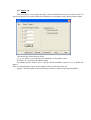
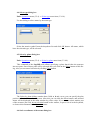
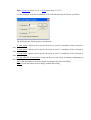
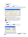
1.3 Uninstalling
Click the "Start" button; select "Settings", then "Control Panel".
The Control panel will be displayed. Click the "Add/Remove Programs" icon.
Locate "SageMD" in the application list and click it. SageMD will be removed
from your system.
2 Mainframe problems and methods, implemented in SageMD
2.1 About program
Molecular dynamics (MD) is widely used to study materials structure and properties based
on the microscopic (atomic scale) models. The range of possible applications for MD simulation
is very broad and is constantly growing with the advances in computer power and accessibility.
Beside classical monographs (see, for example, refs. 1, 2, 3, 4) that describe in detail the theoretical
and algorithmic foundations of MD, there exist numerous applications and computer codes (see
for example refs. 5, 6, 7). The advent of massively parallel computers immensely expanded the
range of possible applications of MD. It is currently feasible to study ensembles of 10 7 ÷ 10 8 atoms/simple molecules with the MD approaches.
SageMD is specifically targeted at modeling materials with the wide range of chemical
bonding situations, including metallic, covalent and ionic bonds. The goal was to make SageMD
a multipurpose, flexible and user-friendly package easy to use in a typical computing environment. The major part of the code is written in FORTRAN 90, while some modules are written in
MS VC++. Graphical User Interface (GUI) simplifies user interaction with the code and provides
for setup of initial data via intuitive and easy to operate dialogues and menus. Initial data, results,
parameters, MD cell, and crystal lattice can be inspected on the computer screen. User-friendly
GUI also allows for analysis of results with a variety of graphs and tools. GUI gives the next
main features:
• 3-D visualization of the periodic atomic structures.
• Copying, moving, deletion, and changing types of the highlighted atoms.
• Highlighting the crystal lattice fragments as boxes, spheres, and cylinders.
• Visualization of rotations and displacements.
• Calculations of bonds lengths and angles between atoms.
• Visualization of orthogonal and perspective projections.
• Exporting atom coordinates to .car, .fdf, .xtl, and .xyz file formats.
• Support for dynamic visualization of modeling results while calculations are running.
SageMD code can be used to model properties of materials at constant temperature and/or
constant pressure, to study behavior of the crystal lattice under expansion or compression, to calculate Radial Distribution Function (RDF), and to derive atomic diffusion coefficients. The user
can choose different boundary conditions, namely: periodical boundary conditions, free surfaces,
and movable walls. In addition, the QEq approach for interatomic energy calculation, which
takes into account atomic charge distribution, has been incorporated into SageMD code for modeling the properties of materials with covalent chemical bonds. For derivation of atomic charges
and other parameters of force fields used in SageMD, quantum chemical programs (e.g.
GAUSSIAN8, ABINIT9, and SIESTA10 ) have been used.
2.2 Molecular Dynamics. Some of the theory
2.2.1 Principles of MD simulation
In classical dynamics the motion is fully determined if a Hamiltonian is known for the system. Hamilton equations (1) determine the ensemble evolution11, 12.
dqi ∂ H (q, p )
=
,
dt
∂ pi
(1)
dpi
∂ H ( q, p )
=−
, i = 1,2....N .
dt
∂ qi
For the ensemble of structureless particles interacting with each other via an effective potential that depends only on their mutual position, the generalized coordinates, and momenta, the
Hamiltonian is determined by the following relations:
q i ≡ ri , p i ≡ m vi , H (r , p ) =
N
∑
p i2
+ U (r ),
2m
(2)
where U (r ) is the total potential energy of the ensemble of particles under consideration.
Note, U (r ) depends only on the spatial coordinates of the particles r ≡ ( r1 , r2 , K rN ) . Hence, the
system of equations (1) is given by
i =1
dri
= vi ,
dt
dv
∂U (r )
.
m i =−
dt
∂ ri
By introducing the force that affects the particle with a number i , Fi = −
(3)
∂U ( r )
, the system
∂ ri
of equations (2) can be rewritten as:
dri
= vi ,
dt
dv
m i = Fi
dt
(4)
i = 1,2....N .
For the additive pairwise interactions, the equations of motion are given by
dri
= vi ,
dt
dv
m i = ∑ Fi j , i = 1,2....N ,
dt
j ≠i
(5)
where Fi j is an interaction force between particles i and j .
Adiabatic approximation (the Born-Oppenheimer approximation13) further allows us to describe interatomic interactions via effective potentials.
The classic equation of motion (3) can be used to describe the state of microparticles (atoms and molecules) if λ << a , where λ is the de Broglie wavelength for a particle and a is the
typical distance between particles. De Broglie’s wavelength for the particle with the mass m
( m = µ ⋅ M u ) is determined by the relation:
2π h 2
.
(6)
µ ⋅ M u ⋅k T
Taking into account the values of the fundamental constants14 Planck constant, Boltzmann
λ=
constant, and unit of atomic mass:
h = 1.0546 ⋅ 10 −34 J ⋅ s, k = 1.3807 ⋅ 10 − 23 J / K ,
T ~ 300K, the equation (6) can be written as:
1
λ ≅
,
M u = 1.6605 ⋅ 10 − 27 kg , for temperature
µ
(7)
where is µ is the atomic or molecular mass of the particle.
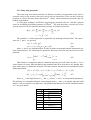
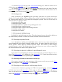
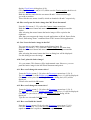
Table 1 contains calculated values of the relation λ / a for some metals and gases. For
metals the value of a represents the interatomic interaction between the nearest neighbors in a
crystal lattice under normal conditions. For gases the value of a is related to the σ parameter in
the Lennard-Jones interparticle potential. The numerical values of parameters a and σ were
taken from refs. 14 and15.
Substance
C (diamond)
Al
Cu
W
Ar
N2
H2
a, Å
1.544
2.863
2.556
2.741
3.418
3.749
2.968
Molecular or atomic
mass, µ , g/mole
12.011
26.981
63.546
183.85
39.948
28.013
2.016
λ /a
0.187
6.72. 10-2
4.91. 10-2
2.69. 10-2
4.63. 10-2
5.034 10-2
0.237
Table 1. Numerical values of relation of the de Broglie wave length to the typical interatomic distance.
As can be seen from the results given in Table 1, the expression λ / a << 1 is satisfied for
metals. At the room and higher temperatures this condition is also satisfied for many gases.
The trajectories and velocities of particles calculated by solving equations (3) provide information about the thermodynamic and kinetic properties of a substance. The thermodynamic
parameters of a substance (macroscopic parameters) in the classical statistical physics are determined from mean ensemble values of the respective dynamic functions, Aobser. = 〈 A〉 . Symbol
〈.....〉 denotes the ensemble averaging for the dynamic function A(q, p ) with respect to coordinates and momenta. The ergodic hypothesis16 is used to calculate Aobser . from the velocities and
trajectories:
t
1
〈 A〉 = lim ∫ A[v(τ ), r (τ )] dτ
t →∞ t
0
(8)
2.2.2 Approaches to numerical solution of the equations of motion
There are several established methods for numerical solution of equations of motion in molecular dynamics. We will describe the ones implemented in the SAGE MD code. One of the
early methods for numerical solution of the equations of motion in MD simulations was the Ver-
let method17,
given by:
18
for which the difference equations for the particle coordinates and velocities are
r (t + ∆t ) = 2r (t ) − r (t − ∆t ) + a (t ) ⋅ (∆t ) 2 ,
v(t ) = [r (t + ∆t ) − r (t − ∆t )] / 2∆t.
(9)
In terms of computer time and memory, the most effective method is the ‘leap-frog’ approach1. The difference equations are given here by:
v(t + 0.5∆t ) = v(t − 0.5∆t ) + a (t ) ⋅ ∆t ,
r (t + ∆t ) = r (t ) + v(t + 0.5∆t ) ⋅ ∆t.
(10)
The particle velocities at time t can be calculated from the equation
v(t ) = [v(t + 0.5∆t ) + v(t − 0.5∆t )] / 2 .
(11)
Velocity Verlet method19 was also derived. It allows the calculation of coordinates and particle velocities in one time step. The difference equations for this case are given by:
r (t + ∆t ) = r (t ) + v(t ) ⋅ ∆t + 0.5 ⋅ a (t ) ⋅ (∆t ) 2 ,
v(t + ∆t ) = v(t ) + 0.5 ⋅ [a (t ) + a (t + ∆t )] ⋅ ∆t.
(12)
This approach, however, requires that acceleration vectors for two time steps are stored in
the computer memory. SageMD code uses this approach1 to calculate the velocity vector. The
velocity vector is calculated in two steps. At first the intermediate value of velocity is calculated
v(t + 0.5∆t ) = v(t ) + 0.5 ⋅ a(t ) ⋅ ∆t ,
(13)
and, at the second step, the new acceleration vector a(t + ∆t ) is calculated and stored in the
computer memory utilizing the already unneeded array, which was freed after previously storing
the acceleration vector a(t ) . Subsequently, velocity values at the time moment t + ∆t are calculated from equation:
v(t + ∆t ) = v(t + 0.5∆t ) + 0.5 ⋅ a(t + ∆t ) ⋅ ∆t.
(14)
The total size of the arrays necessary to implement this algorithm is 9⋅N, where N is the
number of particles. To calculate the amount of required computer memory it is necessary to
multiply this number by the number by the size of the computer word. In SageMD these arrays
are of type double precision type, i.e. each array element takes 8 bytes. The main advantage of
this algorithm is that particle coordinates and velocities are calculated at the same time step. This
method, like all methods considered here, is the second-order method. The Gear and Beeman
algorithms1 are also implemented in the SageMD code for numerical solution of the equations of
motion.
2.2.3 Optimal choice of the method to integrate equations of motion
The most accurate of the above integration methods is the Gear method. However, it requires a large amount of computer memory. The testing done for integration methods showed
that the Gear method gives the lowest fluctuations of the total energy as compared to the other
two methods. However, to hold the total energy at constant value, the size of the integration step
needs to be smaller than for Verlet or Beeman approach. This leads to the increase of computer
time needed to conduct the MD simulation. The fluctuations of the total energy in the Beeman
method are much smaller than in the Verlet method, while the requirements to the integration
step are almost the same. However, Beeman method requires more computer memory. Since the
major part of computer time is spent in step where forces are calculated, these methods can be
considered equivalent with respect to computation rate. While Verlet method requires the least
amount of computer memory compared to the other two methods, it causes appreciably larger
fluctuations of the total energy. In SageMD code the velocity Verlet method is used as a default.
Irrespectively of the integration method, however, it is necessary to make sure that the total energy of the system is preserved, or otherwise reduce the integration step. The 'integrator' command is implemented in the code to select the integration method.
2.2.4 MD simulation at constant temperature and constant pressure
The method suggested by Berendsen20 is implemented in SageMD code for simulation at
constant temperature and constant pressure. Temperature control in this approach is achieved by
multiplying atom velocities by a coefficient λ, defined by the following equation:
⎡
⎣
λ= ⎢1 +
∆t
⎤
⋅ (T0 / T − 1)⎥
τ
⎦
1/ 2
,
(15)
where ∆t is the integration time step, τ is the typical relaxation time, T is the current temperature and T0 is the defined fixed temperature.
The pressure is controlled by changing atom coordinates and the size of the MD box. At
every time step atom coordinates and the size of MD box are rescaled by the coefficient µ calculated from the expression:
µ= ⎡⎢1 −
⎣
∆t
⎤
⋅ ( P0 − P )⎥
B ⋅τ
⎦
1/ 3
,
(16)
where ∆t is the integration time step, τ is the relaxation time, P0 is the pressure to be maintained constant, P is the current pressure value in the ensemble of particles and B is the compression bulk modulus. The value of the bulk modulus B need not be precisely equal to the real
value. In SageMD this method is extended to account for the anisotropic case. The size of MD
box can be therefore changed independently in three directions, and in general case the three
components of the pressure tensor Pxx, Pyy, Pzz are specified instead of pressure of the scalar P0.
In this case P0 = (Pxx, + Pyy, + Pzz)/3.
2.3 Interatomic Potentials
2.3.1 Pair Potentials
The choice and derivation of interatomic potential parameters is a central problem in molecular dynamic simulation. The non-empirical intermolecular and interatomic interaction potentials can be developed from the quantum-mechanical theory. The interatomic interaction is determined by the solution of the Schrödinger equation for a system of interacting nuclei and electrons. For the multi-particle system the Schrödinger equation can only be solved approximately.
Important simplification is achieved by separating electronic and nuclear motions via adiabatic
approximation13. The approximate solution of the Schrödinger equation provides the adiabatic
potential for nuclei. This potential is often sufficiently accurate and yields quality values for
properties expressing interaction between atoms and molecules. De novo calculation of the potential for the many-electron system is, however, a complex problem. Therefore semi-empirical
approaches, which contain parameters fitted to the experimental data, are often used in practice.
Due to proximity of atoms in the condensed matter under normal conditions, it is almost
impossible to derive potentials for two-particle interactions from experimental data. Potentials, in
fact, are not the pair potentials but represent effective potentials, which include effects of manyparticle interactions21. These effective potentials are widely used to study properties of liquids
and solids. Such potentials, fitted over a number of experimentally measured characteristics, allow us to calculate (quantitatively or semi-quantitatively) many important crystal properties. The
equation of state, crystal elasticity modulus, adhesion energy, and the crystal structure are the
examples of data used for fitting the parameters that enter effective potentials.
The types of interatomic pair potentials that are incorporated in the SAGE MD code are described below.
Lennard-Jones potential:
n
m
U 0 ⎡ ⎛ r0 ⎞
⎛ r0 ⎞ ⎤
U (r ) =
⋅ ⎢m ⋅ ⎜ ⎟ − n ⋅ ⎜ ⎟ ⎥ ,
n − m ⎢⎣ ⎝ r ⎠
⎝ r ⎠ ⎥⎦
(17)
Morse and Morse modified potential:
U ( r ) = U 0 ⋅ [exp( − 2α ⋅ ( r − r0 )) − 2 exp( −α ⋅ ( r − r0 ))] , (18)
U0
U (r ) =
⋅ [exp( − m α ⋅ ( r − r0 )) − m ⋅ exp( −α ⋅ ( r − r0 ))] , (19)
m −1
Buckingham and Buckingham modified potential:
6
⎡6
⎛
⎞ ⎞ ⎛ r0 ⎞ ⎤
⎛r
⎟
⎜
⋅ ⎢ ⋅ exp − α ⋅ ⎜⎜ − 1⎟⎟ − ⎜ ⎟ ⎥ ,
⎟
⎜
⎢⎣α
⎠ ⎠ ⎝ r ⎠ ⎥⎦
⎝ r0
⎝
n
⎡n
⎛
⎛ r
⎞ ⎞ ⎛ r0 ⎞ ⎤
U0
⋅ ⎢ ⋅ exp⎜ − α ⋅ ⎜⎜ − 1⎟⎟ ⎟ − ⎜ ⎟ ⎥ ,
U (r ) =
⎜
⎟
1 − n / α ⎢⎣α
⎝ r0
⎠ ⎠ ⎝ r ⎠ ⎥⎦
⎝
U0
U (r ) =
1− 6 /α
(20)
(21)
where U 0 is the minimum value of the potential, r0 represents the interatomic distance
when U = U 0 , and n, m, α are additional potential parameters derived from theory or experiment.
Parameters for pair potentials are often derived by fitting the calculated lattice energy at
zero temperature to the crystal sublimation energy, and by optimizing unit cell parameters and
compressibility so they follow experimental data.
The constant temperature metal compression curves are also used for parameter fitting in
the pairwise potentials. Currently the interatomic potential parameters for 26 metals representing
different types of crystal lattices (body-centered, face-centered, hexagonal closed – packed) are
incorporated in the code. Several different properties of metals are quite well reproduced by using these pair potentials, as shown in the recent contributions coming from our group22, 23, 24.
To better represent Coulomb interatomic interactions, the use of variable atomic charges
(reflecting changing atom configurations) has been suggested25. The values of charges are computed with the charge equilibration (QEq) method26 and the short-term interactions are approximated by the two-particle Morse potential. This approach was successfully applied to the simulation of the structure and properties of silicon oxide with four (quartz) and six (stishovite) coordinated silicon, amorphous silicon oxide, and transition of quartz to stishovite. The (QEq) method
has been incorporated in SageMD with potential parameters available for the number of ionic
species. The Ewald summation is used to calculate the Coulomb interaction energy to avoid
problems with necessary cutoff distances for these long-range interactions.
2.3.2 Many body potentials
The many body interaction potentials are different from the pair potentials as the total interaction energy of the system is not just a sum of all pair interactions. There are three main approaches to express the many body interactions27: cluster, cluster functional potentials, and embedded atom method.
In 1985 paper Stillinger and Weber suggested the potential with two- and three-particle
terms for modeling the diamond structure of silicon28. The work describes a special case of the
general expression for the potential interaction energy of N identical particles:
Φ(1,..., N ) = ∑ v1 (i ) + ∑ v2 (i, j ) +
i
∑ v (i, j, k )
i, j
i , j ,k
i< j
i< j <k
3
(22)
+ ⋅ ⋅ ⋅ + vN (1,..., N )
The potential v1 in this expression is responsible for modeling external forces. The expressions for v2 and v3 are given by
(23)
v2 (ri j ) = ε f 2 (ri j σ ) ,
v3 (ri , rj , rk ) = ε f 3 (ri σ , rj σ , rk σ ) ,
(24)
where ε and σ are introduced here in order to make the potential and the interatomic distance dimensionless. The following five-parameter function is used for the pairwise term of the
potential:
⎧
⎛ 1 ⎞
−p
−q
⎟, r < a
⎪ A (B r − r )exp⎜
f 2 (r ) = ⎨
(25)
⎝r−a⎠
⎪0,
r≥a
⎩
This function is continuous and has continuous derivatives for all orders at point a . It is a
useful feature for many MD-calculations that potential and all its derivatives are smooth functions with respect to coordinates of atoms. The three particle interactions are calculated from the
following formula:
f 3 (ri , r j , rk ) = h(ri j , ri k ,θ j i k ) + h(rj i , rj k ,θ i j k ) + h(rk i , rk j ,θ i k j ) , (26)
where θ j i k
2
⎛ γ
1⎞
γ ⎞⎟ ⎛
(27)
h(ri j , ri k ,θ j i k ) = λ exp⎜
cos(θ j i k ) + ⎟ ,
+
⎜
⎜ ri j − a ri k − a ⎟ ⎝
3
⎠
⎠
⎝
is the angle between ri j and ri k vectors; λ and γ are the potential parameters.
The function h is calculated when the vector lengths (both ri j and ri k ) are smaller than the cutoff
radius a , and it is equal to zero otherwise. The potential parameters for silicon obtained from the
ref.28 are given below:
A
B
p
q
a
λ
γ
σ
ε
7.049556277
0.6022245584
4
0
1.8
21.0
1.2
o
2.0951 A
2.167374937 eV
Stillinger and Weber28 conducted molecular dynamic calculations to model the silicon
properties, in particular, silicon melting temperature. The potential, which they suggested, provides good description of the crystal silicon but it cannot be applied to the non-tetrahedral crystals formed at high pressures. Moreover, this approach was unable to provide an accurate estimate of the phase transfer temperature and the crystal cohesive energy when used with the single
common set of parameters.
In the cluster functional method, the interaction energy is represented as:
Φ = ∑ Φ n (i, j; k ∈ a n ).
(28)
i> j
Each pair of interacting particles i, j is considered a part of the cluster a n composed of n
particles. The cluster configuration depends on the molecular structure. Interaction energy between two particles i and j depends not only upon their own coordinates but also on the coordinates of all n − 2 particles in the a n cluster. Tersoff potential is a typical example of a potential
based on the cluster functional method.
The many-particle potentials suggested by Tersoff29, 30 are widely used for modeling silicon
and other covalent materials. Here, the energy is calculated as a sum of pseudo-pair interactions
with the attraction term being dependent on the local environment of the atom via the bond order
factor:
1
(29)
E = ∑ Ei = ∑ Vij
2 i≠ j
i
(30)
Vij = f C (rij ){aij f R (rij ) + bij f A (rij )}.
where E is the total energy consisting of individual pair contributions, Vij . The repulsive
f R (r ) and the attractive f A (r ) forces are approximated by exponential functions, similar to the
Morse potential:
f R (r ) = A exp(− λ1r ) ,
f A (r ) = − B exp(− λ2 r ) ,
(31)
(32)
⎧1,
⎪
⎪ 1 1 ⎡π
⎤
f C (r ) = ⎨ − sin ⎢ (r − R ) / D ⎥,
⎦
⎪2 2 ⎣ 2
⎪⎩0,
r < R − D,
R − D < r < R + D,
(33)
r > R + D.
Function f C (r ) confines the interactions to be within the “atomic radius”, which greatly
reduces computational effort.
Bond order parameters, aij and bij , are the monotonic functions of the coordination number
of atoms and depend on the valence angle ( θ ijk ) with the neighboring atoms29:
aij = 1 + α nηijn
(
)
η ij =
ik
C
bij = 1 + β nζ ijn
ζ ij =
,
∑ f (r ) exp{λ (r
k ( ≠i , j )
(
−1 / 2 n
)
−1 / 2 n
3
3
ij
3
,
f (r )g (θ )exp{λ (r
∑
( )
k ≠i , j
C
ik
ijk
}
− rik ) ,
3
3
ij
}
− rik ) ,
3
(34)
{
}
g (θ ) = 1 + c 2 / d 2 − c 2 / d 2 + (h − cos θ ) .
2
Tersoff potential works for a wider range of modeling needs than the potential introduced
earlier by Stillinger and Weber28. This does not, however, come without a price. Tersoff potential
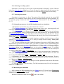
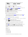
is difficult to parameterize in the complex angular part and generally suffers from the large number of empirical parameters needed. The table below lists two sets of potential parameters for Si
as suggested by Tersoff: version A provides a better description of surface properties, while version B models better elastic properties.
Table 2. Numerical values of the Tersoff potential parameters
A(eV )
B (eV )
⎛
0
⎞
λ1 ⎜⎜ A−1 ⎟⎟
⎝
⎠
0
⎛
⎞
λ1 ⎜⎜ A −1 ⎟⎟
⎝
⎠
α
β
1
Si(A)
3.2647x103
9.5373x101
Si(B)
1.8308x103
4.7118x102
3.2394
2.4799
1.3258
1.7322
0.0
3.3675x10-
0.0
1.0999x10-
n
2.2956x101
c
d
4.8381
2.0417
n
0.0000
⎛
0
⎞
λ3 ⎜⎜ A −1 ⎟⎟
⎝
⎠
o
⎛ ⎞
R⎜A⎟
⎝ ⎠
⎛o⎞
D⎜ A ⎟
⎝ ⎠
6
1
7.8734x10-
1.0039x105
1.6218x101
5.9826x10-1
1.3258
1.7322
3.0
2.85
0.2
0.15
SageMD also incorporates the modifications of the Stillinger-Weber potential as suggested
by Watanabe et al31. These are used to model properties of silicon, silicon oxide, and the interface between these materials. These potential parameters were obtained from quantum-chemical
calculations.
In the embedded atom method (EAM) total energy is represented as follows32:
Φ = ∑ Φ 2 (ri , r j ) + ∑ F (ρ i ),
i> j
(35)
i
where Φ 2 is the pair interatomic interaction energy,
F ( ρ i ) is the energy of atom i embedded in the environment with the electron density ρ i
created by the electrons of all other atoms of the system and considered to be additive:
ρ i = ∑ ρ (rij ) .
j ≠i
(36)
Here, ρ ( r ) is the density of electrons in the atom at the distance r from the nucleus. The
function ρ ( r ) for the given element is derived either from quantum-chemical calculations or
from empirical information. Functions Φ ( ri , r j ) and F ( ρ ) are selected such as to obtain agreement of calculated values with experimental data for a crystal (lattice constant, elastic constants,
sublimation energy, and the vacancy formation energy). The following functional form of F ( ρ )
is universally used for all metals:
F ( ρ ) = −cρ 1 / 2 .
(37)
It allows one to interpret the ρ ( r ) as an overlap integral of wave functions of atoms i and
j . The embedded atom method is successfully used to study structures of metals and alloys, as
well as investigation of crystal lattice defects, surface structures, etc. The (ЕАМ) method in
SAGE MD was extended for 23 elements33.
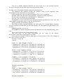
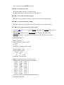
2.3.3 EAM potential file format
The example of the EAM potential file is shown below. This format is similar to one used
XMD code (http://www.ims.uconn.edu/centers/simul/#xmd).
# Johnson's potential for Au *
# cutoff = 5.700 A
*
#Time step determined for fcc Au, 200K (P. Chantrenne)
#DTIME=1.28e-14 s
#Lattice constant 4.08 A.
eunit eV
PAIR 1 1 3000 1 5.7000
1.529143e+02 1.520779e+02 1.512460e+02
1.504188e+02 1.495960e+02 1.487778e+02
1.479640e+02 1.471547e+02 1.463498e+02
...
DENS 1 3000 1 5.7000
5.041442e+01 5.025043e+01 5.008697e+01
4.992404e+01 4.976164e+01 4.959977e+01
4.943842e+01 4.927760e+01 4.911731e+01
...
EMBED 1 400 0 40
0.000000
-0.090532
-0.179980
...
Lines beginning with the sign (#) are comments and must be placed at the beginning of the
file.
The "eunit" command sets energy units for the potential. It can be eV, K and erg. If this
command do not present in the file, the energy units are eV.
PAIR type1 type2 table_size distance1 distance2
The pair or PAIR command identifies the table below as a pair potential function.
The type1 and type2 are the atom types involved in the interaction.
The table_size is the number of points in the pair potential tables.
The distance1 and distance2 define the distance range in the angstrom units.
The distance2 is the cutoff radius for the potential.
In the example above the pair table has distances from 1 to 5.7 angstroms.
The first value in the pair table corresponds the 1 angstrom of atoms separation.
The last value corresponds the cutoff distance (5.7 angstroms).
After the "pair" line is the pair potential table.
The number of values in the table must match the number specified in the "pair" line. The
values must be separated by spaces or the new line characters.
DENS type table_size distance1 distance2
The DENS or dens command identifies the table below as a electron density function.
The type specifies to which atom type the table belongs. The other parameters the same as in the
pair line.
EMBED type table_size ro1 ro2
The EMBED or embed command identifies the table below as the embedded energy functions.
The ro1 and ro2 define the electron density range.
The first value of the table corresponds the ro1 value of the density,
the last value of the table corresponds the r02 value.
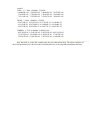
If the structure contains 2 different atom types you must prepare 3 files. The example of
these files is below. (NiAl alloy)
The nial_ni_ni.pot file.
eunit K
PAIR 1 1 3000 1.000000 4.789502
0.000000E+00 9.146377E+05 9.097009E+05 9.047881E+05
8.998996E+05 8.950352E+05 8.901946E+05 8.853778E+05
8.805849E+05 8.758153E+05 8.710694E+05 8.663468E+05
...
DENS 1 3000 1.000000 4.789501
0.000000E+00 3.775296E-25 3.770337E-25 3.765355E-25
3.760348E-25 3.755318E-25 3.750264E-25 3.745187E-25
3.740086E-25 3.734963E-25 3.729817E-25 3.724649E-25
...
EMBED 1 2362 0.0000000 1.705184e-24
-1.137440E-13 -7.041029E+02 -9.087178E+02 -1.037061E+03
-1.127587E+03 -1.194739E+03 -1.245699E+03 -1.284611E+03
-1.314099E+03 -1.335936E+03 -1.351383E+03 -1.361368E+03
...
The nial_ni_al.pot file.
eunit K
PAIR 1 2 3000 1.100000 5.463932
6.850880E+05 5.270333E+05 5.237156E+05 5.204156E+05
5.171331E+05 5.138681E+05 5.106205E+05 5.073902E+05
5.041770E+05 5.009810E+05 4.978020E+05 4.946400E+05
...
The nial_al_al.pot file.
eunit K
PAIR 2 2 3000 1.000000 5.554982
0.000000E+00 7.524923E+05 7.480864E+05 7.437026E+05
7.393409E+05 7.350010E+05 7.306829E+05 7.263866E+05
7.221119E+05 7.178585E+05 7.136267E+05 7.094161E+05
...
DENS 2 3000 1.000000 5.554981
4.567510E-11 4.321021E-25 4.317819E-25 4.314566E-25
4.311262E-25 4.307906E-25 4.304500E-25 4.301044E-25
4.297538E-25 4.293982E-25 4.290377E-25 4.286722E-25
...
EMBED 2 2213 0.000000 2.054483e-24
-8.057838E-14 -5.634532E+02 -5.423222E+02 -4.451216E+02
-3.138738E+02 -1.632606E+02 -1.056015E-01 1.718979E+02
3.505433E+02 5.344154E+02 7.225567E+02 9.142900E+02
...
Note that nial_ni_al.pot file contains only the pair interaction table. The other examples of
the EAM potentials you can find in the EAM subdirectory of the SageMD installation directory.
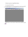
3 The Basic Operations of SageMD Main Window
3.1 Starting SageMD. Main Window
Click the Start button, move the mouse pointer sequentially to Programs then to SageMD,
and click SageMD. SageMD will start and the SageMD main window will be displayed.
Alternative method – from My Computer or Windows Explorer, double-click SageMD
icon
.
3.2 SageMD main window menus
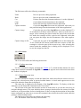
3.2.1 File menu
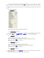
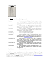
The File menu offers the following commands:
New
Open
Close
Save
Save As
Export
Import
ConvToUnix
Print
Print Preview
Print Setup
Exit
3.2.2 Edit menu
Creates a new document.
Opens an existing document.
Closes an opened document.
Saves an opened document using the same file name.
Saves an opened document to a specified file name.
Saves an opened document to a specified file format.
Opens a document using a specified file format.
Converts a WIN/DOS text file to a Unix text file format.
Prints a document.
Displays the document on the screen, as it would appear printed.
Selects a printer and printer connection.
Exits SageMD
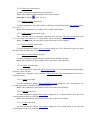
The Edit menu offers the following commands:
Undo
Redo
Cut
Copy
Paste
Capture window
Reverse previous editing operation.
Reverse previous undo command action.
Deletes data from the document and moves it to the clipboard.
Copies data from the document to the clipboard.
Pastes data from the clipboard into the document.
Copies the SageMD screen onto the clipboard. After that you
can paste the image into the documents of the other applications.
Capture image
Copies the any part of the SageMD screen to the clipboard. To
do it hold the left mouse button and move mouse to draw the rectangle. After releasing the mouse button the part of the screen that
lies inside the rectangle will be copied to the clipboard. After that
you can paste the image into the documents of the other applications.
Capture image to file
Copies the any part of the SageMD screen to the bitmap file.
To do it hold the left mouse button and move mouse to draw the
rectangle to select the part of the screen to save. After releasing the
mouse button the standard Save as dialog will be displayed. Use it
to save the image into the file.
3.2.3 View menu
The View menu offers the following menu items:
3.2.3.1 Toolbar menu item
Use this command to display and hide the Toolbar (3.3), which includes buttons for some
of the most common commands in SageMD. A check mark appears next to the menu item when
the Toolbar is displayed.
3.2.3.2 Status Bar menu item
Use this command to display or hide the Status Bar, which describes the action to be executed by the selected menu item or pressed toolbar button. A check mark appears next to the
menu item when the Status Bar is displayed.
The status bar is displayed at the bottom of the SageMD window. To display or hide the
status bar, use the Status Bar command in the View menu.
The left area of the status bar describes actions of menu items as you use the arrow keys to
navigate through menus. This area similarly shows messages that describe the actions of toolbar
buttons as you depress them, before releasing them. If after viewing the description of the toolbar
button command you wish not to execute the command, then release the mouse button while the
pointer is off the toolbar button.
The right areas of the status bar indicate the following:
Sel= The number of the currently selected atoms.
N= The number of atoms in the lattice
3.2.4 Display menu
The Display menu offers the menu items:
3.2.4.1 Parameters menu item
Parameters menu item opens Display parameters dialog box (4.1), which allows you to
build the atoms bonds and control the appearance of the OpenGL objects.
Note: This command is not available if there are no atoms.
3.2.4.2 Zoom menu item
Use this command to magnify or miniaturize the structure image on your screen. Hold the
left mouse button and move mouse in the direction indicated by the mouse pointer to increase or
decrease the structure image. Hold the right mouse button to rotate the image. To cancel this
command uncheck the Zoom menu item or use the toolbar shortcut. To fit the structure image to
the screen press the spacebar.
Note: This command is not available if there are no atoms.
Shortcuts: toolbar:
3.2.5 Lattice menu
The Lattice menu offers the following menu items:
3.2.5.1 Create menu item
Use this command to display the Lattice Builder dialog box (4.2), which allows you to
build or rebuild the crystal.
Note: This command is not available if the Lattice Builder dialog is opened.
Shortcuts: Toolbar:
3.2.5.2 Delete menu item
Use this command to delete the current structure.
Note: The command is not available if there is not a structure.
Shortcuts: Keys:Ctrl+Del
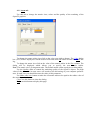
3.2.5.3 Add from file menu item
Use this command to display the standard Open dialog box. Use it to locate the *.vnd file
on your computer or network from which you wish extract the structure and add to the existing
one.
Note: Only the atoms will be added. The unit cell parameters and other data will be not
changed.
3.2.6 Operations menu
The Operations menu offers the following menu items:
3.2.6.1 Select geom... menu item
Use this command to open Select geom… dialog box (4.3), which allows you to select the
atoms using the Box (4.3.1), Sphere (4.3.2) and Cylinder (4.3.3) tabs of this dialog box.
3.2.6.2 Select all menu item
Use this command to select all atoms of the structure.
Note: This command is not available if all atoms have already been selected.
Shortcuts: Toolbar:
; keys: CTRL+A
3.2.6.3 Select none menu item
Use this command to deselect all atoms of the structure.
Note: This command is not available if there are no the selected atoms.
Shortcuts: Toolbar:
; keys: SHIFT+A
3.2.6.4 Select type menu item
Use this command to display Select type dialog box (4.4), which allows you to select the
atoms by the atom type.
Note: This command is not available if there are no atoms.
3.2.6.5 Select invert menu item
Use this command to toggle the current selection.
Note: This command is not available if there are no atoms.
Shortcuts: Toolbar:
; keys: ALT+A
3.2.6.6 Select volumes menu item
Use this command to select all volumes, which have been defined using Set volumes dialog
box (4.17).
Note: This command is not available if no volumes are defined.
3.2.6.7 Select fixed atoms menu items
This command allows to select the atoms that were fixed by Add fixed atoms menu item
(3.2.7.10) in the Task menu (3.2.7). These atoms will be selected by yellow color.
Note: This command is not available if the fixed atoms were not added.
3.2.6.8 Select by plane menu items
Use this command to display Select by plane dialog box (4.5), allowing to specify a plane
that divide the structure into two parts.
3.2.6.9 Show selected only menu item
Use this command to display only the selected atoms and hide all other.
Note: This command is not available if there are not the selected atoms.
3.2.6.10 Show all menu item
Use this command to cancel the Show selected only (3.2.6.9) command action and display
all atoms of the structure.
Note: This command is not available if Show selected only command has not been executed previously.
3.2.6.11 Scale menu item
Use this command to display Scale coordinate of atom dialog box (4.6), which allows you
to scale the atomic coordinates of the selected atoms.
Note: This command is not available if there are no the selected atoms.
3.2.6.12 Move menu item
Use this command to display Move atoms dialog box (4.7), which allows you to move the
selected atoms to the new positions.
Note: This command is not available if there are no the selected atoms
3.2.6.13 Copy menu item
Use this command to display Copy atoms dialog box (4.8), which allows you to copy the
selected atoms to the new positions.
Note: This command is not available if there are no the selected atoms.
3.2.6.14 Set type menu item
Use this command to display Set type dialog box (4.9), which allows you to set the new
type to the selected atoms.
Note: This command is not available if there are no the selected atoms.
3.2.6.15 Delete menu item
Use this command to delete the currently selected atoms.
This command is not available if there are no the selected atoms.
Shortcuts: keys:Del
3.2.6.16 Check lattice menu item
Use this command to display Check lattice dialog box (4.10), which allows you to measure
the atoms separation, the angles between atoms and the torsion angles.
Note: This command is not available if Check lattice dialog box is open.
3.2.6.17 Add atom menu item
Use this command to display Add atom dialog box (4.11), which allows you to add new
atom to the structure. Also, you can use List and edit atoms position dialog box (4.12) to add atoms to the current structure.
Note: This command is not available if Add atom dialog box or List and edit atoms position dialog box is open.
3.2.6.18 Edit atoms menu item
Use this command to display List and edit atoms position dialog box (4.12), which allows
you to view and edit the atomic position and types. Also, it allows you to add and remove the
atoms.
Note: This command is not available if List and edit atoms position dialog or Add atom
dialog are open.
3.2.6.19 Add bonds menu item
To add the bond hold the shift key and click the two atoms whose bond you wish to build.
Note: This command is not available if the Auto rebuild check box of the Bond tab (4.1.2)
of the Display Parameters dialog box (4.1) is checked.
Shortcuts: toolbar:
3.2.6.20 Remove bonds menu item
To remove the bond hold the shift key and click the bond, which you wish to remove.
Note: This command is not available if the Auto rebuild check box of the Bond tab (4.1.2)
in the Display Parameters dialog box (4.1) is checked.
Shortcuts: toolbar:
3.2.7 Tasks menu
The Tasks menu offers the following menu items:
3.2.7.1 Wall potential menu item
Use this command to display Set potential for wall dialog box (4.13), which allows you to
specify the potential parameters for the walls used in the MD simulation.
Note: This command is not available while the MD simulation is running.
3.2.7.2 Set potential menu item
Use this command to display Set potential dialog box (4.14), which allows you to specify
the potential and the potential parameters for the interatomic interaction for the MD simulation.
Note: This command is not available while the MD simulation is running or there are no
atoms.
3.2.7.3 Ewald sum menu item
Use this command to display Set Ewald sum parameters dialog box (4.15), which allows
you to specify the Ewald sum parameters.
Note: This command is not available while the MD simulation is running or there are no
atoms.
3.2.7.4 qEq menu item
Use this command to display Set qEq parameters dialog box (4.16), which allows you to
use the qEq model in the current MD simulation.
Note: This command is not available while the MD simulation is running or there are no
atoms.
3.2.7.5 Set volumes menu item
Use this command to display Set volumes dialog box (4.17), which allows you to select the
volumes, where you can calculate the thermodynamic parameters.
Note: This command is not available while the MD simulation is running or there are no
atoms.
3.2.7.6 Boundary cond… menu item
Use this command to display Set boundary condition dialog box (4.18), which allows you
to set the boundary condition for the MD simulation.
Note: This command is not available while the MD simulation is running or there are no
atoms.
Shortcuts: Toolbar:
3.2.7.7 Shock waves menu item
Use this command to open the Shock waves dialog box (4.19), which allows you to set the
direction and value of the velocity of the selected atoms. You will be able also to define the step
at which apply this velocity.
Note: This command is not available if the simulation is running or number of atoms is 0.
3.2.7.8 Run… menu item
Use this command to display Set parameters for run dialog box (4.20), which allows you to
specify the MD simulation parameters such as the time step, the number of the time steps, the
output options and start the simulation.
Note: This command is not available while the MD simulation is running or there are no
atoms.
Shortcuts: Toolbar:
3.2.7.9 Reset menu item
Use this command to delete the current document and open the last saved version of the
document. When the MD simulation is running you can use this command to abort simulation or
detach the simulation process from the GUI shell. After finishing the MD simulations you must
to do this command otherwise some commands will be unavailable.
Note: This command is not available if the new document has not been saved yet.
Shortcuts: Toolbar:
3.2.7.10 Add fixed atoms menu item
This command allows “to freeze” the group of the selected atoms in the current MD simulation. The coordinates of these atoms will not be changed during the whole simulation. To fix
atoms you must select wanted group of atoms and click once on this menu item.
Note: This command is not available if no atoms were selected.
3.2.7.11 Unfix atoms menu item
This command allows "to unfreeze" all atoms which were fixed by Add fixed atoms
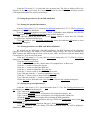
(3.2.7.10) command.
Note: This command is not available if no atoms were fixed.
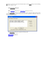
3.2.8 Results menu
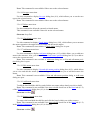
The Results menu offers the following commands:
Lentview
Graph Rdf
Graph Msd
Graph Temp
Graph Energy
Graph Stress
Graph Stress vol
Graph Temp vol
Graph Velocity
Graph Lattice
Use this command to display the Lentview program's dialog,
which allows you to view the changes of the structure during
simulation process. This command is available only after simulation is done.
Allows viewing the radial distribution function (RDF)
graph, of the selected volume. This graph is not available if before
simulation any volume was not selected.
Allows viewing the mean-square deviation (MSD) function
graph, of the selected volume. This graph is not available if before
simulation any volume was not selected.
Allows viewing the Temperature graph.
Allows viewing the total Energy graph.
Allows viewing the graphs of the external Pressure and its
components Px, Py, Pz. This graph is available if the stress calculation during the MD simulation was turned on [to turn on stress
calculation use the Set parameters for run dialog box (4.20)].
Allows viewing the external Pressure and its components
graphs of the selected volumes. This graph is available if the
stress calculation during the MD simulation was turned on and
before MD simulation volume was selected.
Allows to view the temperature graph of the selected volumes, This graph is not available if before simulation any volume
was not selected.
Allows viewing the Velocity components graphs Vx, Vy,
Vz. This graph is not available if before simulation any volume
was not selected.
This command allows viewing 3D Lattice structure.
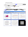
The Graphs … menu items allow you to view all necessary graphs (Temperature, Energy,
Pressure, Velocity, MSD and RDF) after the current MD simulation is done. The time step of all
graphs depends on value Save step parameter, which may specified in the Set parameters for run
dialog box (4.20). You can easily manipulate with this data, copy to the MS Excel or MS Word,
change the axis, line, titles properties and so on.
Set Graph Title dialog box (4.21)
Axis dialog box (4.22)
Line dialog box (4.23)
Allows to change graph and axis titles and
fonts. To open this dialog double click on the desired
title.
Allows to change axis properties. To open this
dialog double click on the desired axis.
Allows to change graph line style. To open this
dialog double click on the desired line
To copy the graphs data to the MS Excel activate the graph window and use Ctrl + C keyboard shortcut. Start MS Excel and use Ctrl + V shortcut to paste the graph data on MS Excel
sheet. To paste the graph to MS Word use “Paste special” command from the “Edit” menu of
this application.
3.2.9 Graph menu
The Graph menu offers the following commands:
Temperature
Volumes Temp
Allows viewing the Temperature graph.
Allows viewing the temperature graph of the selected
volume.
The all aforesaid in the preview section about manipulating with graphical data and setting
graph’s properties is correctly for this graphs.
3.3 SageMD main window Toolbar
The toolbar is displayed across the top of the application window, below the menu bar. The
toolbar provides quick mouse access to many tools used in SageMD,
To hide or display the Toolbar, choose Toolbar from the View menu (ALT, V, T).
ClickTo
Open a new document.
Open an existing document. SageMD displays the Open dialog box, in which you
can locate and open the desired file.
Save the active document or template with its current name. If you have not
named the document, SageMD displays the Save As dialog box.
Print the active document.
Remove selected data from the document and stores it on the clipboard.
Copy the selection to the clipboard.
Insert the contents of the clipboard into the SageMD document.
Reverse the last editing.
Reverse the last undo command action.
Create or rebuild the crystal.
Delete the current document and open the last saved version of the document.
Set the boundary condition for the MD simulation.
Run the MD simulation.
Zoom the lattice image.
Select all atoms.
Deselect all atoms.
Toggle the selection.
Add the bond manually.
Remove the bond manually.
4 Dialog Boxes
The most of menu items opens the various dialog boxes that allow entering input data and
setting essential parameters. The base dialog boxes itemize below in this chapter. All dialog
boxes were extracted into the individual chapter for both hyperlinks and text references usability.
So, this chapter may be omitted in User Manual reading.
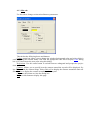
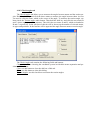
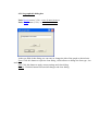
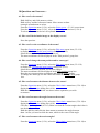
4.1 Display parameters dialog box
Path: Display menu (3.2.4) → Parameters menu item (3.2.4.1).
Use this dialog box to build the atomic bonds and to control the atoms size and colors.
Also, the dialog allows you to change the appearance the bonds and their radiuses. Using this
dialog you can show or hide the bonds and choose the background color. The Display parameters
dialog has the following tabs and buttons:
Atom tab (4.1.1)
Bond tab (4.1.2)
Misc tab (4.1.3)
Close: use this button to close the dialog.
Help: use this button to get the help about the currently active tab.
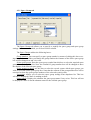
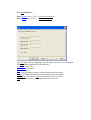
4.1.1 Atom tab
Use this tab to change the atomic sizes, colors and the quality of the rendering of the
OpenGL graphics.
To change the atoms colors just click on the color you wish to change. The Color dialog
box (4.25) will be displayed. Pick the desired color and click OK button to close the Color dialog.
To change the atoms size click on the value of the atomic radius in the Size column. The
dialog will be displayed which allows you to specify the new atomic radius.
Note: The atomic size is in Angstrom units. The default atomic radius equals its covalent radius.
Use the Quality slider to control the rendering quality of the OpenGL objects. The high
value of this parameter in some cases will results to the decreasing of your computer performance. In such case you should decrease the value of this parameter.
Use Make same size button to make the all atomic radiuses be equal to the radius value of
the currently selected atom.
Close: use this button to close the dialog.
Help: use this button to display this page.
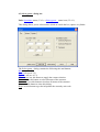
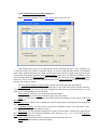
4.1.2 Bond tab
Use this tab to build the atoms bonds, change bonds radius, show or hide the bonds image.
This tab has the following boxes and buttons:
Build bonds: group box allows you to create bonds between two atoms if the following criteria is met:
min factor * covalent radiuses sum < distance < max factor * covalent radiuses sum
where distance= distance between the two atoms forming the bond. To build the bonds click the
Build button. If no bonds are shown try another values of the min and max factors.
Display bonds as cylinder: Check this box to display the bonds as a cylinder. Uncheck this
box to display the bonds as a cone.
Note: If the atoms forming the bond have the same size the bonds will be displayed as a
cylinder in both cases.
Bond radius: Allows you to specify the bond radius as a fraction of the radius of the atoms
forming the bond. If these atoms have different radiuses the minimal radius will be used to display the bond thickness. The bond radiuses are in 0-1 range.
Show bonds: Check this box to display the bond images or uncheck to hide it.
Auto rebuild Uncheck this box to build or remove bonds manually. How to add or remove
bonds manually see Add bonds (3.2.6.19) and Remove bonds (3.2.6.20) menu items.
Close: use this button to close the dialog.
Help: use this button to display this page.
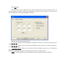
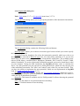
4.1.3 Misc tab
Use this tab to change various miscellaneous parameters.
This tab has the following boxes and buttons:
Colors: group box allows you to change the window background color and color which is
used to display the selected atoms. Just click the appropriate color box to display Color dialog
box (4.25) and choose the new color using this dialog.
Projections: Use this radio button to switch between orthogonal and perspective projections.
Contour: Allows you to specify how the contour around the crystal will be displayed. Select Hide to hide the contour image. Select Unit cell to display the contour around the unit cell.
Select lattice to display the contour around the whole crystal.
Close: use this button to close the dialog box.
Help: use this button to display this page.
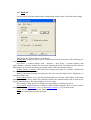
4.2 Lattice Builder dialog box
Path: Lattice menu (3.2.5) → Create menu item (3.2.5.1).
You can use the Lattice Builder dialog to create new crystal, to modify the space group
number, the unit cell parameters, the primitive cell vectors and the box size. Also, using Lattice
Builder dialog box you can add, remove atoms from the unit cell or change their types.
The Lattice Builder dialog contains the following tabs and buttons:
Space Groups tab (4.2.1)
Cell tab (4.2.2)
Asymmetric Cell tab (4.2.3)
Cell vectors tab (4.2.4)
Unit Cell tab (4.2.5)
SuperCell tab (4.2.6)
OK: use this button to build or rebuild the crystal using the data from the dialog tabs and to
close the dialog.
Cancel: use this button to close the dialog without the building or rebuilding the crystal.
Apply Now: the same as OK but the dialog will not be closed.
Help: use this button to get the help about the active tab.
New: if this radio button is checked the current crystal will be deleted before the new crystal will be built.
Add to existing: if this radio button is checked the atoms of the existing structure will not
be deleted. New atoms will be added to the existing atoms. However, the existing unit cell settings will be replaced new one.
4.2.1 Space Group tab
The Space Groups tab allows you to specify or modify the space group and space group
settings for the structure which you wish to build or rebuild.
The Space Groups tab has the following boxes:
Group number: You can specify a space group number by means of editing this box or using the spin buttons. When you change the group number the contents of the Select space group
box will be changed too and vice versa.
Select space group: Enter the space group symbol into this box or select the required space
group from the dropdown list. Note: the contents of group number box will be changed to show
the number of the selected space group.
Select groups to show: use this box to select the crystal system which space groups you
wish to see in the Select space group box. Note that the contents of the group number box will be
restricted to show the space groups numbers of the selected crystal system.
Extensions: Allows you to select the space group settings from dropdown list. This box
will not be displayed if there is nothing to show.
Other names: Displays the alternate the space group name if any exists. This box will not
be displayed if there is not the alternate name for the selected space group.
4.2.2 Cell Tab
The Cell tab allows you to specify the length and relative orientation of the unit cell vectors
in space. The whole crystal can be built by means of the translation of the unit cell along the directions of the unit cell vectors (see SuperCell tab). The space group symmetry can constrain the
lattice parameters to predefined values. In such cases some parameters will not be available to
edit.
a, b, c: The length of the unit cell vectors a, b, c.
alpha: The angle between b and c vectors.
beta: The angle between a and c vectors.
gamma: The angle between a and b vectors.
Crystal system: Can be one of the seven crystal systems (triclinic, monoclinic, orthorhombic, tetragonal, trigonal, hexagonal or cubic. Some of the space groups of the trigonal crystal system can have extensions such as hexagonal or rhombohedral axes.
4.2.3 Asymmetric Cell Tab
Asymmetric Cell tab allows you to build the full unit cell by means of applying the space
group symmetry operations for the each atom in the asymmetric cell. It results to the decreasing
the amount of the work you need to do for the building of the crystal. Some unit cells contain
more then 100 atoms, but asymmetric cell needed to create such unit cell may contain a few atoms only. To build the crystal the SageMD uses the data from Cell (4.2.2), Unit Cell (4.2.5) and
SuperCell (4.2.6) tabs. The Space Groups (4.2.1) and this tabs need to build the unit cell only. In
fact you can define the position of atoms in the unit cell manually. Then you need to define the
cell vectors using the Cell (4.2.2) tab and specify how many times to repeat the unit cell along
cell vectors using the SuperCell (4.2.6) tab, then press OK button to build the crystal.
Asymmetric Cell tab has the following data fields:
Atom positions(fractional): Displays the position and type for the each atom in the asymmetric cell. To edit the atom position or type you can click on the corresponding row in this
field.
Edit positions: Allows you to modify the atom positions. x, y and z are the fractional coordinates of the atom. Their values must be a numbers between 0 and 1. If you specify the other
value the error message will be displayed.
Change Atom: Allows you to modify the current atom type by selecting the new atom from
the dropdown list.
Add Atom: Displays the Pick element (4.25) dialog which allows you to add the new atom
to the asymmetric cell. The default coordinate of the atom are x=0, y=0, z=0. Use the Edit positions boxes to modify these values.
Delete Atom: Click this button to remove an atom from the asymmetric cell
Clear: Click this button to remove all the atoms from the asymmetric cell.
Build unit cell: Click this button to build the full unit cell. The number of atoms and their
positions in the unit cell depend on the space group settings [see Space Group tab (4.2.1)].
4.2.4 Cell vectors tab
Use this tab to see the unit cell vectors. The edit boxes of this dialog have the read only
permission. To edit the unit cell vectors you can use the Cell (4.2.2) tab.
ax, ay, az, bx, by, bz, cx, cy, cz: are the Cartesian components of the a, b, c unit cell vectors.
4.2.5 Unit cell tab
Unit Cell tab allows you to view and edit atoms positions in the unit cell. Also, you can
change the atom type and add atoms to or remove from the unit cell. Generally, you build the
unit cell using the Asymmetric Cell (4.2.3) tab. Alternatively you can define the atom positions
and their types using this tab. In this case you do not require knowing the space group information and asymmetric cell settings.
The Unit Cell tab has the following data fields:
Atom positions (fractional): Displays the position and type for the each atom in the unit
cell. To edit the atom position or type you can click on the corresponding row in this field.
Edit positions: Allows you to modify the atom positions. x, y and z are the fractional coordinates of the atom. Their values must be a numbers between 0 and 1. If you specify the other
value the error message will be displayed.
Change Atom: Allows you to modify the current atom type by selecting the new atom from
the dropdown list.
Add Atom: Displays the Pick element (4.25) dialog which allows you to add the new atom
to the unit cell. The default coordinate of the atom are x=0, y=0, z=0. Use the Edit positions
boxes to modify these values.
Delete Atom: Click this button to remove an atom from the unit cell.
Clear: Click this button to remove all the atoms from the unit cell.
4.2.6 SuperCell tab
The SuperCell tab allows you to create a supercell (crystal) from the current unit cell. Also,
you can use this tab to rebuild the supercell. You define the size of the supercell in terms of the
numbers of the unit cell in each direction. The fractional coordinates of the supercell are in terms
of the unit cell vectors. For example, the fractional coordinates of atoms in 2x2x2 supercell are
in 0-1.9999... range. The atoms in the original unit cell have their coordinates in 0-0.9999...
range.
The SuperCell tab has the following fields:
Number of unit cell in a direction: Allows you to specify the range of the supercell along
the vector of the unit cell.
Number of unit cell in b direction: Allows you to specify the range of the supercell along
the b vector of the unit cell.
Number of unit cell in c direction: Allows you to specify the range of the supercell along
the c vector of the unit cell.
Box size: Defines the periodic box size for MD simulation.
Allow me to change box size manually: By default the box size coincide with the corresponding values in the left box. Check this box to define the box size manually.
4.3 Select geom... dialog box
Path: Operations menu (3.2.6) → Select geom… menu item (3.2.6.1).
This dialog allows you to select atoms, which are inside the box, sphere or cylinder.
The Select geom... dialog contains the following tabs and buttons:
Box tab (see 4.3.1)
Sphere tab (see 4.3.2)
Cylinder tab (see 4.3.3)
Select invert: use this button to toggle the current selection.
Select all: use this button to select all atoms of the structure.
Select none: use this button to deselect all atoms of the structure.
Close: use this button to close this dialog.
Help: use this button to get the help about the currently active tab.
4.3.1 Box tab
This tab allows you to specify the box, which contains the atoms you wish to select. To
specify the box you need to define the coordinates of the two vertex of this box. These vertexes
are the end points of the largest diagonal of the box.
This tab has the following data fields:
X1, Y1, Z1: Allows you to specify the coordinates of the first vertex in the currently active
coordinate system.
X2, Y2, Z2: Allows you to specify the coordinates of the second vertex in the currently active coordinate system.
Coordinate system: Allows you to specify which coordinate system to use to define the
box.
Note: the reduced factor equals to the length of the a vector of the unit cell.
Apply: Click this button to select the atoms, which are inside of the specified box.
4.3.2 Sphere tab
This tab allows you to specify the sphere, which contains the atoms you wish to select. To
specify the sphere you need to define the coordinates of the sphere center and the sphere radius.
This tab has the following data fields:
xc, yc, zc: Allows you to specify the coordinates of the sphere center.
R: Allows you to specify the sphere radius.
Coordinate system: Allows you to specify which coordinate system to use to define the
sphere.
Note: the reduced factor equals to the length of the a vector of the unit cell.
Apply: Click this button to select the atoms, which are inside of the specified sphere.
4.3.3 Cylinder tab
This tab allows you to specify the cylinder, which contains the atoms you wish to select. To
specify the cylinder you need to define the cylinder axis, the coordinates of the cylinder base
center, the cylinder radius and height.
This tab has the following data fields:
Axis along z: Allows you to select from dropdown list the axis along which the cylinder
will be orientated.
xc, yc, zc: Allows you to specify the coordinates of the cylinder base center.
R: Allows you to specify the cylinder radius.
H: Allows you to specify the cylinder height.
Coordinate system: Allows you to specify which coordinate system to use to define the
sphere.
Note: the reduced factor equals to the length of the a vector of the unit cell.
Apply: Click this button to select the atoms, which are inside of the specified cylinder.
4.4 Select type dialog box
Path: Operations menu (3.2.6) → Select type menu item (3.2.6.4).
Use this dialog to select atoms by the atom type.
Select the atomic symbol from the dropdown list and click OK button. All atoms, which
have the selected type, will be selected.
4.5 Select by plane dialog box
Path: Operations menu (3.2.6) → Select by plane menu item (3.2.6.8).
This command of the SageMD code allows specifying a plane that divides the structure
into tow parts. One of these parts will be selected after you click on the Select button of this dialog. Also you can cancel selection by clicking Close button.
The Select by plane dialog contains three fields a, b and c were you can specify the plan
position in fractional coordinate system. After this you can click the Select button, and selected
atoms will be displayed in the main window by yellow color. If you want to select another part
of the structure just click Invert selection button on the toolbar, or press Alt+A in the keyboard,
or choose this command in the Operation menu.
4.6 Scale coordinates of the atoms dialog box
Path: Operations menu (3.2.6) → Scale menu item (3.2.6.11).
Use this dialog to scale the coordinates of the selected atoms by the factors you define.
The dialog has the following boxes and buttons:
X scale factor: Allows you to specify the factor to scale X coordinates of the selected atoms.
Y scale factor: Allows you to specify the factor to scale Y coordinates of the selected atoms.
Z scale factor: Allows you to specify the factor to scale Z coordinates of the selected atoms.
use the same for all directions: Check this box to scale all the coordinate components by
the same factor.
OK: Click this button to scale the atomic coordinates and close the dialog.
Cancel Click this button to close dialog without the scaling.
4.7 Move atoms dialog box
Path: Operations menu (3.2.6) → Move menu item (3.2.6.12).
Use this dialog to move selected atoms by the shift vector you define. All the vector components are in the fractional coordinate system. x is directed along the a, y along the b, z along c
vectors of the unit cell.
The dialog has the following boxes and buttons:
X shift: Allows you to specify the shift along a vector of the unit cell.
Y shift: Allows you to specify the shift along b vector of the unit cell.
Z shift: Allows you to specify the shift along c vector of the unit cell.
use the same for all directions: Check this box to move the selected atoms by the same shift
in all directions.
OK: Click this button to move the selected atoms and close the dialog.
Cancel: Click this button to close dialog without the moving.
4.8 Copy atoms dialog box
Path: Operations menu (3.2.6) → Copy menu item (3.2.6.13).
This dialog allows you to translate the selected group of atoms in any direction and repeat
the displacement one or more times. All the displacement vector components are in the fractional
coordinate system. X is directed along a, y along b, z along c vectors of the unit cell.
The dialog has the following boxes and buttons:
a: Allows you to specify the shift along the a vector of the unit cell.
b: Allows you to specify the shift along the b vector of the unit cell.
c: Allows you to specify the shift along the c vector of the unit cell.
rep: Allows you to specify how many times to repeat this operations.
OK: Click this button to copy the selected atoms and close the dialog.
Cancel: Click this button to close dialog without the copying.
4.9 Set type dialog box
Path: Operations menu (3.2.6) → Set type menu item (3.2.6.14).
Use this dialog to set the type, which you define to the selected atoms.
Select the atomic symbol from the dropdown list or click New Type button to display Pick
element (4.24) dialog, which allows you to pick the new atom type from the table. Then click
OK button to set the new type to the all selected atoms or click Cancel button to close the dialog
without the setting new type.
4.10 Check lattice dialog box
Path: Operations menu (3.2.6) → Check lattice menu item (3.2.6.16).
The Check lattice dialog box allows to measure atoms separation, angels between atoms
and the torsion angels. You can see the positions and atoms separation in fractional, reduced or
Cartesian coordinate systems.
The Check lattice dialog box contains the following tabs:
Check Distance tab (4.11.1)
Check Angels tab (4.11.2)
4.10.1 Check distance tab
The Check distance tab allows you to measure the atoms separation. Hold the shift key and
click the two atoms whose separation you wish to measure. In the edit box of this tab will be
shown up the number of selected atoms, its types and positions. In the third line will be appeared
the atoms separation.
The Check distance tab contains the following fields and buttons:
Chose units: allow you to choose the coordinate system in which the atoms separation and
positions will be shown.
Clear: use this button to clear the edit box of this tab.
Close: use this button to close this dialog.
4.10.2 Check angles tab
The Check Angles tab allows you to measure the angles between atoms and the torsion angles. Hold the shift key and click the three atoms to measure the angle between them. At first
you need to click the atom, which is the vertex of the angle. To measure the torsion angle you
must check the Torsion angles radio button. Then hold the shift key and click the two atoms B
and C whose angle you wish to measure. Then click the two atoms A and D, which are bonded to
B and C respectively. In the edit box of this tab will be shown up the number of selected atoms,
its types and positions. In the last line will be appeared the angle between atoms or torsion angle.
The Check Angles tab contains the following fields and buttons:
Chose units: allows choosing the coordinate system in which the atoms separation and positions will be shown.
Clear: use this button to clear the edit box of this tab.
Close: use this button to close this dialog.
Torsion angels: use this check box to measure the torsion angles.
4.11 Add atoms dialog box
Path: Operations menu (3.2.6) → Add atoms menu item (3.2.6.17).
The Add atom dialog allows you to add new atom to the structure. You can specify the
atomic positions and type.
The Add atoms dialog contains the following fields and buttons:
Edit positions: Allows you to modify the atom positions.
Coordinate system: Use this field to choose the coordinate system. You can choose Cartesian,
reduced
or
fractional
coordinate
system.
Note: the reduced factor equals to the length of a vector of the unit cell.
Change Atom: Allows you to modify the current atom type by selecting the new atom from
the dropdown list.
Add: Use this button to add the new atom to the structure.
Close: Click this button to close this dialog.
4.12 List and edit atoms position dialog box
Path: Operations menu (3.2.6) → Edit atoms menu item(3.2.6.16).
This dialog allows you to view and edit the atomic position and types. Also, it allows you
to add and remove the atoms. Using this dialog you can see and edit the position of individual
atom in the opened document. Just click on the atom in the structure image and you can see the
selected line with atomic position in the Atom positions field. You can edit the coordinates of the
selected atom using the Edit positions boxes and change the atom type using Change atom dropdown list. Also you can select the individual atom in the Atom positions field and it will be selected in the structure image.
The List and edit atoms position dialog contains the following fields and buttons:
Atom positions: Displays the position and type for the each atom of the current structure.
To see the location of the atom in structure image or to edit the atom position and type you can
click on the corresponding row in this field.
Edit positions: Allows you to modify the atom positions.
Note: you need to click Apply button to apply your edit action.
Apply: Use this button to change the atom position accordingly to the values in the Edit
positions boxes.
Change atom: Allows you to modify the current atom type by selecting the new atom from
the dropdown list.
Coordinate system: Use this field to choose the coordinate system. You can choose Cartesian, reduced or fractional coordinate system.
Add Atom: Use this button to add the new atom to the structure. Atom type is specified in
the Change atom box. The default coordinate of the atom are x=0, y=0, z=0. Use the Edit positions boxes to modify these values.
Delete Atom: Click this button to remove an atom from the unit cell.
Close: Click this button to close this dialog.
4.13 Set potential for wall dialog box
Path: Tasks menu (3.2.7) → Wall potential menu item (3.2.7.1).
The Set potential for wall dialog allow you to specify the parameters of the Morse potential
U(r)=u*[exp(-2*Alfa*(r-R0))-2*exp(-Alfa*(r-R0))] on the box walls.
The Set potential for wall dialog contains the following fields and buttons:
U: Allows you to specify the deep of the potential pit.
Alfa: Allows you to specify the hardness parameter of the Morse potential.
R0: The distance r to the point where the potential has the minimum value (U(r)=-u).
Cutoff: Allows you to specify the cutoff radius as the fraction of the R0. The real cutoff radius (Angstrom) is cutoff*R0.
OK: Click this button to set potential parameters for wall and close the dialog.
Cancel: Click this button to close the dialog without saving the wall potential parameters.
4.14 Set potential dialog box
Path: Tasks menu (3.2.7) → Set potential menu item (3.2.7.2).
The Set potential dialog allows you to specify the potentials of the interatomic interactions.
The Set potential dialog contains the following fields and buttons:
Between types: Allows you to choose two atoms types between which you want to specify
the interatomic potential.
Potential: From the dropdown list select the interatomic potential, which you wish to set
for the pair, you selected in Between types box. For many body potentials or if you use the
Ewald sum you must set the same potential for all interatomic interactions. The available potentials are EAM, Morse , modified Morse, Bukingem, Watanabe, SW ,Tersoff B, Tersoff C, BKS,
Abinit, Gaussian98. To use the Abinit and Gaussian98 potentials you need to install these codes
on your computer. During the MD simulations the SageMD call those codes to calculate the
forces. Any pair potential you can represent as EAM potential file, which has only the pair part
of the interatomic interaction. The "dens" and "embed" parts of the file you must exclude. Thus,
you have the ability to implement the pair potentials, which are not implemented in SageMD
code. See EAM potential file format (2.3.3).
Properties: Click this button to display the Set potential parameters dialog box (4.14.1),
which allows specifying the potential parameters of the interatomic interactions. This button is
visible not for all interatomic potentials.
Poten file: This button is available only for EAM potential. It allows choosing the potential
data file.
OK: Click this button to set potential and close the dialog.
Cancel: Click this button to close the dialog.
4.14.1 Set potential parameters dialog box
Path: Tasks menu (3.2.7) → Set potential menu item (3.2.7.2) → Set potential dialog box
(4.14)
The Set potential parameters dialog box allows you to specify selected potential parameters. The next figure represents Set potential parameters dialog box for Morse potential.
4.15 Set Ewald sum parameters dialog box
Path: Tasks menu (3.2.7) → Ewald sum menu item (3.2.7.3).
The Set Ewald sum parameters dialog box allows you to specify long-range electrostatic
potentials methods and to set some parameters.
The Set Ewald sum parameters dialog contains the following fields:
Use Ewald sum: Check this box to use Ewald summation in the current simulation. The
Ewald summation is the technique for calculating electrostatic interactions in a periodic (or
pseudo-periodic) system.
Use direct coulomb summation: Check this box to use direct Coulomb sum in the current
simulation. Use of the direct Coulomb sum is sometimes necessary for accurate simulation of
isolated (nonperiodic) systems. It is not for periodic systems.
Calculate: Click this button to use automatic calculation of Alfa, KMAX, KMAY, KMAZ
parameters. You can enter only Cutoff parameter to use automatic calculation or you can manually specify Alfa, KMAX, KMAY, KMAZ. This button is visible only if use Ewald sum box was
checked.
Edit Charges field: Allows you to choose the atom type and specify its charges.
Cutoff: Allows you to specify the real space cutoff forces Radius of long-range correction.
Alfa: Allows you to specify the Ewald convergence parameter Alfa.
KMAX, KMAY, KMAZ: Allows you to specify the Ewald sum parameters that effectively
define the range of the reciprocal space sum (one for each of the three axis directions).
There are three variables that control the accuracy the Ewald summation, they are - Alfa
the Ewald convergence parameter, Cutoff the real space forces cutoff and the KMAX,Y,Z integers that effectively define the range of the reciprocal space sum (one integer for each of the
three axis directions). These variables are not independent and it is usual to regard one of them
as pre-determined and adjust the other two accordingly. The Ewald sum splits the (electrostatic)
sum for the infinite, periodic system into a damped real space sum and a reciprocal space sum.
The rate of convergence of both sums is governed by Alfa. Evaluation of the real space sum is
truncated at r=Cutoff so it is important that Alfa be chosen so that contributions to the real space
sum are negligible for terms with r>Cutoff. The recommended value for Alfa is 3.2/Cutoff or
greater (too large a value will make the reciprocal space sum very slowly convergent). The optimum values for KMAX are the smallest values that reproduce the correct Coulombic energy and
virial at the value of Alfa to be used in the simulation. Note that one needs to specify the three
integers (KMAX, KMAY, KMAZ) referring to the three spatial directions, to ensure the reciprocal space sum is equally accurate in all directions. The values of (KMAX, KMAY, KMAZ) must
be commensurate with the cell geometry to ensure the same minimum wavelength is used in all
directions. For a cubic cell set KMAX=KMAY=KMAZ. However, for example, in a cell with
dimensions 2A=2B=C (i.e. a tetragonal cell, longer in the c direction than the a and b directions)
use 2KMAX=2KMAY=KMAZ. If the values for the KMAX used are too small, the Ewald sum
will produce spurious results. If values that are too large are used, the results will be correct but
the calculation will consume unnecessary amounts of cpu time. The amount of cpu time increases with KMAX*KMAY*KMAZ.
4.16 Set QEq parameters dialog box
Path: Tasks menu (3.2.7) → qEq menu item (3.2.7.4).
Use this dialog box to turn on the QEq method for the MD simulation. Rappe and Goddard
III suggested the charge equilibration (QEq) model to predict the atoms charge distribution in
dependence of the molecular geometry.
The dialog has the following fields and buttons:
Use qEq: check this box to use the qEq method during the MD simulation.
Call qeq every N step: means that every N step the atomic charges will be recalculated.
OK: click this button to apply current settings and close dialog.
Cancel: Click this button to discard all changes and close dialog.
The parameters of the QEq model are in the QEq_params.dat file. The example of such file
is following below.
#*********************************************************
#El QuanNo MinQ MaxQ ElectNeg Hardness GenRadii
H
1 -1 1 4.52800 6.49205 0.37100
Li
2 -1 1 3.00600 2.38600 1.55700
C
2 -4 4 5.34300 5.06300 0.75900
N
2 -3 5 6.89900 5.88000 0.71500
O
2 -2 6 8.74100 6.68200 0.66900
F
2 -1 7 10.87400 7.47400 0.70600
Na
3 -1 1 2.84300 2.29600 2.08500
Mg
3 -1 2 3.95100 3.69300 1.50000
Al
3 -5 3 4.06000 3.59000 1.20100
Si
3 -4 4 4.16800 3.48700 1.17600
P
3 -3 5 5.46300 4.00000 1.10200
S
3 -2 6 6.92800 4.48600 1.04700
Cl
3 -1 7 8.56400 4.94600 0.99400
K
4 -1 1 2.42100 1.92000 2.58600
Br
4 -1 7 7.79000 4.42500 1.14100
Ti
4 -1 4 3.47000 3.38000 1.60700
Zr
5 -1 4 3.40000 3.55000 1.75800
To learn more see original paper 26
4.17 Set Volumes dialog box
Path: Tasks menu (3.2.7) → Set volumes menu item (3.2.7.5).
Set Volumes dialog box allows to select any atoms in the current structure into independent
group, which called volume. These volumes are useful if you want to get some parameters not of
the whole structure, but only of the some part of it. You can add up to 20 volumes. To add new
volume you must select atoms (see the FAQs Q1) and click Add volume button.
The Set volumes dialog contains the following buttons:
Add volume: Allows to add selected group to the new volume.
Delete volume: Allows to delete selected volumes from the volumes list.
Close: Click this button to close Set volumes dialog.
Set volumes dialog realized in tree-type structure. In the root we can see the selected volumes. The second branches (rdf, msd and stress) contain the parameters to the calculation of the
radial distribution function, mean square deviation and stress. To open the second branches click
once on the cross.
RDF - Radial Distribution Function. Radial distribution function is a statistical function
about the atomic distribution around an atom in a structure. This function describes fluctuations
in density around given atom. You can think of it as the average number of atoms found at given
distance in all directions.
The RDF branch contains following parameters:
first_step: Allows to specify the initial time step of RDF calculation.
last_step: Allows to specify the final time step of RDF calculation.
dr: Allows to specify the radial step width of RDF.
Rmax: Allows to specify the maximum value of the RDF radius.
MSD - Mean Square Deviation. The mean square displacement contains information on the
atomic diffusivity
The MSD branch contains following parameters:
first_step: Allows to specify the initial time step of MSD calculation.
last_step: Allows to specify the final time step of MSD calculation.
print_step: Allows to specify the frequency for saving MSD in the trajectory file.
Stress: Not realized yet.
To change or specify any parameter in the RDF, MSD or Stress branches just click once on
the required field end enter your value.
Select and click once on the volume name to rename it (the default name is "NoName"). To
exclude the volume from the current simulation process just double click on the volume's cross
or name (near the name will be appeared red cross instead of green tick).
4.18 Set boundary conditions dialog box
Path: Tasks menu (3.2.7) → Boundary cond… menu item (3.2.7.6).
The Set boundary conditions dialog box allows you to set the boundary conditions for the
MD simulation. By default periodic boundary conditions are in effect - this can be altered with
this dialog. The periodic boundary conditions can be turned off in any direction independently of
the others. When the periodic boundary conditions are turned off in some direction you need to
adjust the position and velocity of the potential wall using the Wall button for this direction.
Thus, you can simulate free surfaces by setting the wall position beyond the wall potential cutoff
distance from the crystal free surface. Also, you can simulate the processes of compression or
tension of the crystal by setting none zero wall velocities.
The dialog has the following fields and buttons:
Box size: Allows you to change the size of the simulation box. This option is not available
if periodic boundary condition is not set.
Periodic boundary: Allows you to set or unset periodic boundary conditions in a, b and c
directions of the unit cell. If in some direction the periodic boundary is turned off you can use the
button below to display Moving wall dialog box (4.18.1), which allows you to set the potential
wall position and velocity.
OK: Use this button to apply your changes and close the dialog.
Cancel: Use this button to discard your changes and close the dialog.
4.18.1 Moving wall dialog box
Path: Tasks menu (3.2.7) → Boundary cond… menu item (3.2.7.6) → Set boundary conditions (4.18) dialog box.
The Moving wall dialog box allows you to set the potential wall at specified distance from
crystal surface.
The dialog has the following fields and buttons:
Walls offset from boundaries: Allows you to specify distance between the crystal edge and
the potential wall in reduced units. Use the left box to specify the distance from the edge, which
is the near coordinate system origin. Use the right box to specify parameters for the opposite
edge of the crystal. The negative values mean that the potential wall was moved in the negative
direction of the coordinate axe from the crystal edge. You specify offset in the reduced units.
Walls velocity: Allows you to specify the value and direction of the wall velocity. Use this
feature to model the crystal tension or compression.
Free surface: Check the box or boxes to model the free surface or surfaces of the crystal.
Use for restart only: Check this box to set wall positions and velocities between restarts of
the MD simulation. By default, the wall positions and velocities between restarts keep values
from previous MD simulation.
OK: Use this button to apply your changes and close the dialog.
Cancel: Use this button to discard your changes and close the dialog
4.19 Shock waves dialog box
Path: Tasks menu (3.2.7) → Shock waves menu item (3.2.7.7).
Use this dialog box to simulate the propagation of the shock waves in the structure or when
you need abruptly to set the new value and direction of the selected atoms velocity (the bombarding processes). The initial velocity value is applied at the beginning the step you specify using this dialog. To add shock wave you must select atoms before clicking on the Add button.
The dialog has the following fields and buttons:
N: The number of the shock wave. You have not the possibility to edit this field.
Name: The name of the shock wave. You can leave the default name or type the new one.
This field must not be empty.
Step: The step number at which apply the specified initial velocity to the atoms, which
were selected for the shock wave. Which atoms were selected you can see by clicking on the desired line. The atoms of the selected wave will be highlighted.
Velocity: the value of the atoms velocity of the shockwave. This value applied as the initial
velocity of the shock wave atoms at the beginning of the specified step. You set velocity using
the reduced units. The real value (km/s) =Velocity*velocity reduced factor.
A, B, C: define the vector in fractional units along which the velocity vector of the shock
wave atoms will be directed. At the example the one shock wave is directed in positive direction
of the A vector of the simulation box and another in the negative direction of this vector. The
value of the vector is no matter. The direction means only. The (1,1,1) and (5,5,5) vectors have
the same direction. So you can specify any of them.
Add: use this button to specify new shock wave from the currently selected atoms.
Del: use this button to delete the currently selected shock wave.
Edit: use this button to change the shock wave parameters. Also, you can double click on
the line you wish to edit.
Close: use this button to close the dialog.
4.20 Set parameters for run dialog box
Path: Tasks menu (3.2.7) → Run… menu item (3.2.7.8).
The Set parameters for run dialog box allow you to specify the MD simulation parameters.
The Set parameters for run dialog contains the following fields and buttons:
General options field:
Time step: Allows you to set the time step interval for performing numerical integration of
the motion equations. The time step interval will be equal to this factor multiplied on Reduced
time unit.
Number steps: Allows you to specify the number of simulation steps.
Initial temperature: Allows you to set the initial temperature of the MD simulation.
Output options field:
Save step: Allows you to specify the frequency for saving of the trajectory files.
Print step: Allows you to specify the frequency for printing and saving other simulation results such as temperature, energy, stresses.
Constant temperature options field:
Const temperature: Check this box to turn on the constant temperature simulation.
Temperature: Allows you to specify the temperature, which will be maintained during the
MD simulation.
Relaxation time: Allows specifying the relaxation time constant. The greater value of this
constant will require to run more steps to reach the desired temperature. However, the small
value of the constant will result in too abrupt changes of the MD quantities. The 100*time_step
value will be the good value to start.
Constant pressure options field:
Constant pressure: Check this box to turn on the constant pressure simulation.
Px, Py, Pz: The Cartesian components of external pressure. The positive value of the pressure will results in compressing the structure. To stretch the structure use the negative value of
the pressure.
Isotropy: Check this box to choose isotropic external pressure simulation. For the nonorthogonal lattices you must check this box.
Relaxation time: Allows setting the relaxation time constant. The more value you set to this
constant the more steps you need to run to reach the desired value of the pressure. However, the
small value of the constant will result in too abrupt changes of the MD quantities. The
100*time_step value will be the good value to start.
Bulk module: Allows you to specify the bulk elastic modulus. The value of the bulk elastic
modulus should not be necessarily equal to exact real value. In most cases you do not need to
change the default value.
Neighbors list options field:
Use Neighbors list: Check this box to use the neighbors list in MD simulation.
Max neighbors: This value is used to build the neighbors list. Increase this value if you receive the error message "the neighbors list too small."
Cutoff factor: All atoms whose separation less then factor*cutoff will be included in the
neighbors list. The cutoff is the potential cutoff radius. The factor must be more 1.
Restart: Check this box to continue the previous MD simulation. You can change some parameters of the MD simulation.
Stress: Check this box to turn on the stress calculation during the MD simulation.
Include thermal stress: Check this box to include the velocity dependent part of the stress
tensor in the stress calculation.
UX: The reduced factor for energy.
RX: The reduced factor for a distance.
AMX: The reduced factor for a mass.
Reduced time unit: The reduced factor for a time. The real time = reduced time*reduced
time unit.
OK: Click this button to start simulation with the current parameters.
Cancel: Click this button to exit the dialog and discard all changes.
4.21 Set graph title dialog box
Path: Results menu (3.2.8) → one of menu items or
Path: Graph menu (3.2.9) → one of menu items.
In the text field of this dialog you can enter or change the title of the graph or desired axis.
Font: Click this button to open the font dialog, which allows to change the font type, size
and color.
OK: Click this button to apply current settings and close dialog.
Cancel: Click this button to discard all changes and close dialog.
4.22 Axis dialog box
Path: Results menu (3.2.8) → one of menu items or
Path: Graph menu (3.2.9) → one of menu items
The Axis dialog allows changing or specifying the axis format, scale and grid.
The Axis dialog contains the following tabs:
Axis Scale tab (4.22.1)
Axis Format tab (4.22.2)
Grid tab (4.22.3)
OK: Click this button to apply current settings and close dialog.
Cancel: Click this button to discard all changes and close dialog.
Apply Now: The same as OK but the dialog will not be closed.
Help: Use this button to get the help about the active tab.
4.22.1 Axis Scale tab
The Axis Scale tab allows changing the axis initial and finite value, the major and minor
division scale factor.
The Axis Scale tab contains the following fields:
Maximum value: Allows changing the axis finite value.
Minimum value: Allows changing the axis initial value.
Major division: Allows changing the major division scale factor.
Minor division: Allows changing the minor division scale factor.
4.22.2 Axis Format tab
The Axis Format tab allows changing the axis style, color and weight.
The Axis Format tab contains the following fields:
Style: Use this box to select the axis line style from dropdown list.
Color: Use this box to select the axis line color from dropdown list.
Weight: Use this box to select the axis line weight from dropdown list.
4.22.3 Grid tab
The Grid tab allows changing the major or minor grid style, color and weight.
The Grid tab contains the following fields:
Style: Use this box to select the major or minor line style from dropdown list.
Color: Use this box to select the major or minor line color from dropdown list.
Weight: Use this box to select the major or minor line weight from dropdown list.
4.23 Line Dialog box
Path: Results menu (3.2.8) → one of menu items or
Path: Graph menu (3.2.9) → one of menu items.
The Line dialog allows changing the graph line style, color and weight.
Style: Use this box to select the graph line style from dropdown list.
Color: Use this box to select the graph line color from dropdown list.
Weight: Use this box to select the graph line weight from dropdown list.
OK: Click this button to apply current settings and close dialog.
Cancel: Click this button to discard all changes and close dialog.
Apply Now: The same as OK but the dialog will not be closed.
Help: Use this button to get the help.
4.24 Pick element dialog box
Use this dialog to pick the element from the periodic table of elements or to see element's
properties. Click on the element symbol button and then click OK button to pick element or click
Properties button to see the elements properties.
4.25 Color dialog box
5 Simulation Executing
5.1 Lattice Building
SageMD is a powerful tool for crystal building. Using the different visualization techniques available in SageMD, you can create high quality graphics that can be easily pasted into
other windows-based software programs or saved as bitmaps.
The next sections describe several ways of the crystal building in SageMD code.
5.1.1 Using the SageMD structure database
SageMD has the structure database that contains many different types of structures. You
can open the desired structure using the File menu (3.2.1) or by pressing the
button on the
toolbar. A standard Open dialog box is displayed on the screen. Locate the SageMD templates
directory (usually .../Program Files /SageMD/Template). Open needed subdirectory, select the
*.vnd file and click the Open button. The structure will be displayed on your screen. Select
Create (3.2.5.1) from Lattice menu (3.2.5) and use Super Cell Tab (4.2.6) in Lattice builder dialog box (4.2.) to rebuild crystal.
5.1.2 Importing crystals into SageMD from others applications.
You can import the files with format different from SageMD. Just open the File menu
(3.2.1) and click on Import item to display on the screen a standard Open dialog box. Choose the
required file format from the dropdown list in the bottom of dialog; select the file and press Open
button. The crystal will be displayed in the SageMD main window.
5.1.3 Building crystal from scratch
There is the consecution of action for building alpha quartz crystal (SiO2) from scratch:
1. Start SageMD.
2. Select New from the File (3.2.1) menu.
3. Select the and then Create (3.2.5.1) menu item of Lattice (3.2.5) menu. The Lattice
Builder dialog (4.2) will be displayed.
4. Under group number enter 154. Make sure that "P3221" is displayed in the Select space
group combo box.
5. Click Cell tab (4.2.2). Enter a=4.914 and c=5.405.
6. Click the Asymmetric Cell tab (4.2.3). Click the Clear button and then the Add Atom
button. The Pick element (4.24) dialog box will be displayed.
7. Click the Si button and then OK.
8. In the Edit positions group box on Asymmetric Cell tab (4.2.3) enter the values:
x=0.4699 y=0 z=0.6666667.
9. Click the Add atom button, choose O and click OK.
10. Enter the position of O atom x=0.4141 y=0.2681 and z=0.7854.
11. Click the Build unit cell button on Asymmetric Cell tab (4.2.3) and then the Unit Cell
tab (4.2.5) on Lattice Builder dialog (4.2). Make sure that the full unit cell contains 9 atoms.
12. Click the Apply Now button and move the dialog to a screen corner. Use the left mouse
button to rotate the lattice and right mouse button to move it.
13. Click the SuperCell tab (4.2.6) on Lattice Builder dialog (4.2). Make the number cell in
all directions equal to 2. Click the OK button.
14. From the File (3.2.1) menu, select the Save as menu item to save your work. The standard Save as dialog box will be displayed. Enter "SiO2" as the file name and then choose the directory to save the file and click the Save button.
5.2 Selecting atoms
Many operations in the SageMD operate upon those atoms that are selected in the main
window (for example adding volumes, adding a layer of the fixed atoms, deleting atoms and so
on). Selected atoms in the 3D view window are displayed in yellow. There are several ways to
select one atom or a group of atoms:
Selecting the individual atom
Selecting the group of atoms.
Selecting the spherical, cylindrical or parallelepipedic areas.
Selecting the atoms according its type.
Selecting the whole structure and inverting selection.
Selecting according a plane.
Selecting the fixed atoms.
5.2.1 Selecting the individual atom
Hold shift key and click atoms to select. The picked atoms become selected, in addition to
any atoms already selected. If an atom was already selected it becomes unselected.
5.2.2 Selecting the group of atoms
As an alternative to picking on an individual atom to select it, one or more atoms may be
selected graphically by drawing a rectangle with the mouse. All atoms within this region are considered "picked". Hold CTRL key and the left mouse button. Move mouse to draw rectangle
around the atoms to select. The starting point of the mouse forms one vertex of the rectangle and
the current location of the mouse is the opposite vertex.
5.2.3 Selecting the spherical, cylindrical or parallelepipedic areas
Some tasks for crystal building or interface constructing needs geometrical figures to be selected. The Select geom... (4.3 ) dialog box of the Operations (3.2.6 ) menu item allows to select
areas with spherical, cylindrical or parallelepipedic form.
5.2.4 Selecting the atoms in concordance with its type.
If you want to select all the same type atoms of the current crystal structure use the Select
type (4.4) dialog box of the Operations (3.2.6) menu item.
5.2.5 Selecting the whole structure and inverting selection.
You can select all atoms by pressing the CTRL+A keyboard buttons, or choose Select all
button on the toolbar.
(3.2.6.2) menu item of the Operations (3.2.6) menu, or click once
Also you can invert your selection by pressing ALT+A, or choosing Select invert (3.2.6.5) menu
item of the Operations (3.2.6) menu or clicking once
button on the toolbar.
5.5.6 Selecting according a plane.
Sometimes it is necessary to select some region that should be limited by a plane. With the
help of the Select by plane dialog box (4.5) you can specify a plane that divides the structure into
two parts. One of the parts will be selected after you click on the Select button of this dialog.
5.5.7 Selecting fixed atoms.
Sometimes it is necessary “to freeze” the group of the selected atoms in the current MD
simulation. The coordinates of these atoms will not be changed during the whole simulation. Select requisite group of atoms and click Add fixed atoms menu item (3.2.7.10) in the Task menu
(3.2.7).
5.3 Setting the parameters for the MD simulation and run simulation
1. Build lattice by one of the ways, described in the section 5.1.
2. Use Display parameters (4.1) dialog to change atoms colors, sizes, rendering quality and
build atom bonds if it is necessary. Menu path: Display → Parameters.
3. Use Set potential (4.14) dialog to set interatomic potential for atoms. You can implement
your own pair potential. To do it you need prepare your own potential file. The format of the file
is EAM potential file format (2.2.4). Only the pair section must be presented in this case. Choose
EAM potential in the Set potential (4.14) dialog box and specify your file as EAM potential file.
Menu path: Tasks → Set potential.
3. Set boundary conditions. The periodic boundary conditions in all direction are default
settings. Use Set boundary conditions (4.17) dialog to change default settings. Menu path:
Tasks->Boundary condition.
4. If you wish calculate the RDF (Radial Distribution Function) or MSD (Mean Square
Displacement) you need to set volumes. Also, you must set volumes if you wish monitoring the
temperature and stresses in some part of the simulation cell. Select atoms, which you wish to insert into a volume and click Set volumes menu item (3.2.7.5) from Tasks (3.2.7) menu to display
Set volumes dialog box (4.17), which allows you to set the volume parameters. To calculate
RDF and MSD for the whole simulation cell select all atoms as the volume. You can create up to
20 volumes. Menu path: Tasks → Set volumes.
5. Use Ewald sum parameters (4.15) dialog box if your pair potential has Coulumb item.
Also, you can use qEq model in this case. However, the number of atoms must be less then 600
to use qEq model. Menu path: Tasks → Ewald sum and Tasks → qEq.
6. Optionally, you can fix the selected atoms positions during MD simulation. The positions of the fixed atoms are not updated during the MD simulation and their velocities will be set
to 0. Menu path: Tasks → Add fixed atoms.
7. Use Set parameters for run (4.20) dialog to set other parameters and start the MD simulation. Menu path: Tasks → Run.
8. Click OK button to close the dialog. The MD simulation script file will be displayed.
Close it to start simulation.
5.4 Monitoring the simulation
After starting the MD simulation click the Graph menu (3.2.9) and select Temperature
menu item, or Volumes Temp menu item if any volumes were selected. You may observe representation of selected quantity on graph.
When the simulation is done click the
icon on the toolbar.
5.5 Viewing the results
Use some of menu items of the Results menu (3.2.8) in concordance with your task to see
graphs. Use Tile vertically menu item of the Windows menu to see all graphs simultaneously. To
scale graphs double click on the desired axis. Double click on the line to change line properties.
Double click on titles to change the title text and font.
You can copy the graphs data to the MS Excel. Activate the graph window and use Ctrl +
C keyboard shortcut to copy the graph to the clipboard. Start MS Excel and use Ctrl + V shortcut
to paste the graph data on MS Excel sheet. To paste the graph to MS Word use “Paste special”
command from the “Edit” menu of this application. The print command will be realized soon.
6 Sources of information – Libraries and Databases
6.1 Database on structures
SageMD database on structures represent the library of ready for use files (with extension
.vnd) that contains unit cell structures for many different elements and crystalline materials. This
library is located in SageMD templates directory (usually .../Program Files /SageMD/Template).
See in section 5.1.1 how to build lattice, using the SageMD structure database.
You may to supplement database by your own unit cell structures. See in section 5.1.3 how
to build unit cell structure, using the SageMD.
6.2 Database on potential parameters
Excuse, it’s not ready now.
7 Tutorial. Melting of the Al crystal
The eam_al.vnd file is the ready for use the project file for this tutorial. You can find it in
the "Template" subdirectory of the SageMD installation directory. However, you need to correct
the path to al.pot file. In this tutorial the path is E:\Program Files\SageMD\EAM\al.pot. If during
installation you choose the default path then you need only to change the drive letter. Save the
project file in the new directory before you start the simulation. All output files will be created in
the directory where you saved the project file.
7.1 Building of the Al crystal
Double-click the SageMd icon on your desktop.
Select Open... from the File menu (3.2.1). The Open file dialog will be displayed.
Locate the SageMD templates directory. (Usually .../Program Files /SageMD/Template).
Open the "elements" subdirectory, select the Al.vnd file and click the Open button. The unit cell
of the Al structure will be displayed.
Click the
icon on the toolbar. The Lattice builder dialog box (4.2) will be displayed.
Click the SuperCell tab (4.2.6). Make the number of unit cell in all directions equals 5 and
click the OK button.
From the File menu (3.2.1), select the Save as menu item. The Save as dialog will be displayed. Use it to save your work. It is recommended you save the file in new directory because
of all input and output files will be located here.
7.2 Setting the parameters for the MD simulation
7.2.1 Setting the potential parameters
From the Tasks menu (3.2.7), select the Set potential menu item (3.2.7.2). The Set potential
dialog box (4.14 ) will be displayed.
From the Potential dropdown list select "EAM" (Embedded Atom Method) and click the
Poten file button. The Set EAM potential file dialog will be displayed.
Type the full path to the al.pot file or use Browse button to locate this file. (Usually
.../Program Files/ SageMD/EAM/al.pot).
Click OK button to close Set EAM potential file dialog box and then OK button to close
Set potential dialog box.
7.2.2 Setting parameters for RDF and MSD calculation.
We wish to run the 3000 steps of the MD simulation. The RDF function will be calculated
using the 500 last steps. The MSD we will calculate using all steps. We wish to calculate the
RDF function and MSD using all atoms of the crystal. Thus, we need to select all atoms. Hold
Ctrl and press C keys to select all atoms.
From the Tasks menu (3.2.7), select the Set volumes menu item (3.2.7.5). The Set volumes
dialog box (4.17) will be displayed.
Click the Add volume button.
Click "NoName" and type the volume name (for example Box1 or Box1.txt).
Click the "+" mark to expand the list tree.
Click the "+" mark to expand the RDF tree.
Click the "+" mark to expand the first_step tree.
Click the "1" box to select it, then click it again to edit.
Type 2500 and click the "+" mark to expand last_step tree.
Click the "1" box to select it, then click it again to edit.
Type 3000 and click the "+" mark to expand Msd tree.
Set the last_step to 3000 and click Close button to close the Set volumes dialog box.
7.2.3 Setting the general parameters.
From the Tasks menu (3.2.7), select Run menu item (3.2.7.8). The Setting parameters for
run dialog box (4.20) will be displayed.
Type 3000 in the number steps box.
Type 10 in the Save step box to set frequency for saving the trajectory file.
Type 10 in the Print step box to set frequency for saving the other output files.
Check the Stress checkbox to output stresses during the MD simulation.
Check the Const temperature checkbox and type 1500 in the Temperature and 1 in the Relaxation time boxes.
Check the Const pressure checkbox and type 1 in the Relaxation time box.
Click OK button to close the dialog. The MD simulation script file will be displayed.
Close it to start simulation.
7.3 Monitoring the simulation
After starting the MD simulation click the Graph menu (3.2.9) and select Temperature
menu item.
From the Window menu select Tile vertically menu item. You can see the temperature
graph and the aluminum structure simultaneously.
When the simulation is done click the
icon on the toolbar.
7.4 Viewing the results
Use Graph RDF, Graph MSD, Graph temp, Graph energy and Graph stress menu items of
the Results menu (3.2.8) to see graphs. Use Tile vertically menu item of the Windows menu to
see all graphs simultaneously.
8 Final Results – Documents and Files
Excuse, it’s not ready now.
9 How to work with 3D graphics
You can always change the display style of a current structure. Using the options of the
Display parameters dialog, you can control several stylistic features of the structures displayed in
the main window of the SageMD code. Some of the characteristics you control in the Display
parameters dialog are:
The rendering style, size and color of the atomistic structure.
Various parameters of the bonds building.
The color of the background and selected atoms.
The style and form of the contour around the lattice.
The style of viewing atomic structure (orthogonal or perspective).
9.1 The rendering style, size and color of the atomistic structure
The Atom tab (4.1.1) of the Display parameters dialog box (4.1) controls the graphical representation of atoms. Here you can change the atomic sizes, colors and the quality of the rendering of the OpenGL graphics. Fore example, to change the atoms colors just click on the color
you want to change. The Color dialog box (4.25) will be displayed. Pick the desired color and
click OK button to close the Color dialog box. All the structure elements in SageMD are given a
default color, usually defined by the type of atomic element. But sometimes it is useful to give a
custom color to the chosen element.
9.2 Various parameters of the bonds building.
Use Bond tab (4.1.2) on the Display parameters dialog box (4.1) to build the atoms bonds,
change bonds radius, show or hide the bonds image. This tab allows to change parameters for the
whole structure. But if you wish to build several bonds between some atoms you must carry out
the following actions: First, make sure that in the Bond tab (4.1.2) of the Display parameters dialog (4.1) the Auto rebuild check box is unchecked and the Show bonds check box is checked.
Then click the
button on the toolbar. Hold the shift key and click the two atoms whose bond
button in the toolbar and select
you wish to build. If you want to remove bound just click the
this atoms. Also you can use Add bonds (3.2.6.19) and Remove bonds (3.2.6.20) menu items in
the Operations menu (3.2.6).
9.3 The color of the background and selected atoms.
The default color of the background is black. As for selected atoms it is yellow. But you
can change the color manually (for example before capturing and importing atomic structure 3D
view image). You can change these parameters from the Misk tab (4.1.3) of the Display parameters dialog box (4.1).
9.4 The style and form of the contour around the lattice. The style of viewing atomic
structure (orthogonal or perspective).
These two characteristics can be also controlled from the Misk tab (4.1.3) of the Display
parameters dialog box (4.1).
Just choose wanted projection in the projection field. Depending on you choice the projection will be orthogonal or perspective. Also you can specify how the contour around the crystal
will be displayed. Select Hide to hide the contour image. Select Unit cell to display the contour
around the unit cell. Select lattice to display the contour around the whole crystal
10 Questions and Answers…
A1. How can I select atoms?
Hold shift key and click atoms to select.
Hold ctrl key and the left mouse button. Move mouse to draw
rectangle around atoms to select.
From the Operation menu (3.2.6), select the Select geom... (3.2.6.1) menu item.
From the Operation menu (3.2.6), select the Select type menu item (3.2.6.4).
To select all atoms use the ctrl+A keyboard shortcut.
A2. How can I fit the lattice image to the display screen?
Press the spacebar.
A3. How can I see the coordinates of the atoms?
From the Operation menu (3.2.6), select the Edit atoms menu item (3.2.6.18)
to display the List and edit atom position dialog box (4.12).
Select the atom whose position you wish to see.
The atom coordinates will be displayed in the "Edit position" group box.
A4. How can I change the atom position and/or atom type?
From the Operation menu (3.2.6), select the Edit atoms menu item (3.2.6.18)
to display the List and edit atom position dialog box (4.12).
Select the atom whose position you wish to change.
The atom coordinates will be displayed in the Edit position group box.
Enter the new atom position coordinates and click the Apply button.
To change the atom type use the combo box under the Change atom group
box.
A5. How can I measure the distance between the atoms?
From the Operation menu (3.2.6), select the Check lattice menu item (3.2.6.16) to
display the Check lattice dialog box (4.10).
Hold the shift key and click the two atoms whose separation you wish
to measure.
A6. How can I measure the angles between the atoms?
From the Operation menu (3.2.6), select the Check lattice menu item (3.2.6.16) to
display the Check lattice dialog box (4.10).
Click the Check angles tab (4.10.2). Make sure that the Torsion angles check box is
not checked.
Hold the shift key and click the three atoms to measure the angle between
them. At first you need to click the atom, which is the vertex of the angle.
A7. How can I measure the torsion angles?
From the Operation menu (3.2.6), select the Check lattice menu item (3.2.6.16) to
display Check lattice dialog box (4.10).
Click the Check angles tab (4.10.2). Make sure the Torsion angles check box is
checked.
Hold the shift key and click the two atoms B and C whose torsion angle
you wish to measure.
Then click the two atoms A and D, which are bonded to B and C respectively.
A8. How can I paste the lattice image into MS Word document?
From the Edit menu (3.2.2), select the Capture image menu item.
Hold the left mouse button and move mouse to draw rectangle around the
lattice.
After releasing the mouse button the lattice image will be copied to the
clipboard.
After that you can paste the image in such applications as Word, Power Point,
Excel, Paint using “Paste” command from “Edit” menu of this applications.
A9. Can I save the lattice image in the file?
Yes, you can save the lattice image as the bitmap (bmp) file.
From the Edit menu (3.2.2), select the Capture image to file menu item.
Hold the left mouse button and move mouse to draw rectangle around the
lattice.
After releasing the mouse button the Save as dialog box will be displayed.
Use this dialog to save the image.
A10. Can I print the lattice image?
No, you cannot. This feature will be implemented soon. However, you can
paste the lattice image in the MS Word document and print it.
A11. How can I change the atoms colors?
From the Display menu (3.2.4) select the Parameters menu item (3.2.4.1).
The Atom tab (4.1.1) of the Display parameters dialog box (4.1) will be displayed.
Click on the color you wish to change. The Color dialog box (4.25) will be
displayed.
Choose color and click OK button.
A12. How can I change the atoms sizes?
From the Display menu (3.2.4) select the Parameters menu item (3.2.4.1).
The Atom tab (4.1.1) of the Display parameters dialog box (4.1) will be displayed.
Click the size you wish to change. The Change ball size dialog will be
displayed.
Type the new size and click OK button.
A13. How can I build the bonds?
From the Display menu (3.2.4) select the Parameters menu item (3.2.4.1).
Click the Bond tab (4.1.2). If the min factor and max factor have values
equals to zero make it equals to 0.6 and 1.1 respectively.
Click Build button. If no bonds are displayed you need to increase the value
of the max factor. Make sure the Show bonds and Auto rebuild check
boxes are checked.
A14. How can I add/remove the bonds manually?
(add bond) and
(remove bond) toolbar icons are
Make sure that
available.
If it is not then from the Display menu (3.2.4) select the Parameters menu item (3.2.4.1).
Click the Bond tab (4.1.2) and uncheck the Auto rebuild check box.
Make sure that the Show bonds check box is checked.
Click the
icon on the toolbar to build the bonds.
Hold the shift key and click the two atoms whose bond you wish to build.
icon on the toolbar to remove the bonds.
Click the
Hold the shift key and click the bond you wish to remove.
A15. How can I change the background color?
From the "Display" menu select the Parameters menu item (3.2.4.1). Click Misc tab.
Click the background color. The "Choose color" dialog will be displayed.
Choose color and click "OK" button.
A16. How can I hide/show the contour around the lattice?
From the Display menu (3.2.4) menu select the "Parameters..." menu item. Click "Misc"
tab (4.1.3).
Check the Hide radio button to hide the contour.
Check the Unit cell radio button to draw contour around the unit cell.
Check the lattice radio button to draw contour around the crystal.
A17. Can I paste the atoms positions into the Notepad or Word documents?
Yes, you can. Select the atoms whose positions you wish to paste. You can
select all atoms.
From the Edit menu (3.2.2) select Copy or use the ctrl+C keyboard shortcut to copy
the atoms positions to the clipboard. After that you can paste the positions
into the applications using their the "Paste" command from the "Edit" menu.
The following example is the pasting of the SiC cubic unit cell into MS Word
document.
NumberAtoms=8
Si 0 0 0
Si 0 2.174 2.174
Si 2.174 0 2.174
Si 2.174 2.174 0
C 1.087 1.087 1.087
C 1.087 3.261 3.261
C 3.261 3.261 1.087
C 3.261 1.087 3.261
If you place the text in such format to the clipboard then you can paste
these atoms into the SageMD document.
A18. How can I delete atoms?
Select the atoms to delete. Press the Del key.
To delete all atoms use the ctrl+Del keyboard shortcut.
A19. How can I rotate the lattice image?
Hold the left mouse button and move the mouse to rotate the lattice image.
A20. How can I move the lattice image?
Hold the right mouse button and move the mouse to move the lattice image.
A21. How can I export the lattice to Siesta code?
From the File menu (3.2.1) select the Export menu item. The Save as dialog will be
displayed.
Select the fdf extension in the Save as type box. Type the file name in the
File name.
box and save the file. The following example shows the .fdf file generated by
SageMD.
NumberOfAtoms 9
NumberOfSpecies 2
%block Chemical_Species_label
1 14 Si
2 8 O
%endblock Chemical_Species_label
LatticeConstant 1 Ang
%block LatticeVectors
4.2522 -2.455
0
0
4.91
0
0
0 5.402
%endblock LatticeVectors
AtomicCoordinatesFormat ScaledCartesian
%block AtomicCoordinatesAndAtomicSpecies
2.0444 1.1803 0.0000 1
0.6386 1.6669 0.6293 2
3.1279 1.0685 1.1713 2
0.0000 2.5494 1.8007 1
1.1243 3.5235 2.4300 2
3.6136 -0.7881 2.9720 2
2.2078 -1.2747 3.6013 1
2.4893 2.1746 4.2307 2
1.7629 -0.2804 4.7727 2
%endblock AtomicCoordinatesAndAtomicSpecies
#%include default.fdf
Use "include" directives to include the other Siesta data.
References
1
Allen, M.P.; Tildesley, D.J. Computer Simulation of Liquids; Clarendon Press: Oxford,1987.
2
Rapaport, D.C. The Art of Molecular Dynamics Simulation; Cambridge University Press:
Cambridge, 1995.
3
Frenkel, D.; Smit, B. Understanding Molecular Simulation; Academic Press: New York,
1996.
4
Leach, A.R. Molecular Modelling Principe and Applications; Longman: New York, 1996.
5
Molecular Dynamics Software DISCOVER;
http://www.accelrys.com/insight/discover.html.
6
Molecular Dynamics Software MOLDY; http://www.earth.ox.ac.uk/~keith/moldy.
7
Molecular Dynamics Software Materials Explorer;
http://www.cachesoftware.com/pdfs/MEUserGuide_2.0.pdf.
8
Frisch M.J.; Trucks I.W.; Schlegel H.B.; Secures I.E.; Robb M.A.; Cheeseman J.R.;
Zakrzewski, V.I.; Montgomery, J.A.; Stratmann, R.E.; Burant, J.C.; Dapprich, S.; Millam, J.M.;
Daniels, A.D.; Kudin, K.N.; Strain, M.C.; Farkas, O.; Tomasi, J.; Barone, V.; Cossi, M.; Cammi,
R.; Mennucci, B.; Pomelli, C.; Adamo, C.; Clifford, S.; Ochterski, J.; Petersson, I. A.; Ayala,
P.Y.; Cui, Q.; Morokuma, K.; Malick, D. K.; Rabuck,A.D.; Raghavachari, K.; Foresman, J.B.;
Cioslowski, J.; Ortiz, J.V.; Stefanov, B.B.; Liu, I.; Liashenko, A.; Piskorz, P.; Komaromi, I.;
Gomperts, R.; Martin, R.L.; Fox, D.J.; Keith, T.; Al-Laham, M.A.; Peng, C.Y.; Nanayakkara, A.;
Gonzalez, C.; Challacombe, M.; Gill, P.M.W.; Johnson, B.; Chen, W.; Wong, M.W.; Andres,
J.L.; Gonzalez, C.; Head-Gordon, M.; Replogle, E.S.; Pople, J.A.; Gaussian 98, Revision A.3;
Gaussian, Inc.: Pittsburgh, PA, 1998.
9
Abinit new user guide; http://www.abinit.org/ABINIT/Infos_v3.4/new_user_guide.htm.
10
Software of the SIESTA Project;
http://www.uam.es/departamentos/ciencias/fismateriac
/siesta/.
11
Landau, L.D.; Lifshits, Е.М. Theoretical Physics; V.5, Statistical Physics; Nauka: Moscow, 1987.
12
Balesku, R. Equilibrium and non-equilibrium statistical mechanics; V.1, Mir: Moscow,
1978.
13
Landau, L.D.; Lifshits, Е.М. Theoretical Physics.; V.3, Quantum Mechanics. Nonrelativistic Theory; Nauka: Moscow, 1987.
14
Physical values. Reference book, edited by Grigoryev, I.S., Meylikhov,Е.Z. Moscow.:
Energoisdat, 1991.
15
Girshfelder, J.; Kertiss, Ch., Berd, R., Molecular theory of gases and liquids; Inostrannaya Literatura: Moscow, 1961.
16
Cubo, R. Statistical mechanics; Mir: Moscow, 1967.
17
Verlet, L. Phys Rev 1967, 159, 98.
18
Verlet, L. Phys Rev 1968, 165, 201.
19
Swope, W.C.; Andersen, H.C.; Berens, P.H.; Wilson, K.R. J Chem Phys 1982, 76, 637.
(cited from work1 )
20
Berendsen, H.J.C.; Postma, J.P.M.; VanGunstern,W.F.; Di Nola, A.; Haak, J.R. J Chem
Phys 1984, 81, 3684. (cited from work1).
21
Kaplan, I.G. Introduction in the intermolecular interactions theory; Nauka: Moscow,
1982.
22
Selezenev, A.A.; Golubev, V.K.;Ganchuk N.S. Chem Phys Reports 1998, 17, 295.
23
Selezenev, A.A.; Golubev, V.K.; Aleinikov, A.Yu.; Butnev, O.I.; Barabanov, R.A.; Voronin, B.L. In Proceedings of the conference on Shock Compression of Condensed Matter (Part
1); Atlanta, 2001, 374.
24
Golubev, V.K.; Selezenev, A.A. Khimicheskay Fizika, 2002, 21, 61.
25
Demiralp, E.; Cagin, T.; Goddard III, W.A. Phys Rev Lett 1999, 82, 1708.
26
Rappe, A.K.; Goddard III, W.A. J Phys Chem 1991, 95, 3358.
27
Valuyev, А.А.; Kaklugin, А.S.; Norman, G.E. Successes of Chemistry; 1995, 64 (7),
28
Stillinger, F.H.; Weber, T.A. Phys Rev B 1985, 31, 5262.
29
Tersoff, J. Phys Rev B 1988, 37, 6991.
30
Tersoff, J. Phys Rev B 1988, 38, 9902.
643.
31
Watanabe, T.; Fujiwara, H.; Noguchi, H.; Hoshino, T.; Ohdomari, I., Jpn J Appl Phys
1999, 38, L366.
32
Daw, M.S.; Baskes, M.I. Phys Rev B 1984, 29, 6443.
33
Baskes, M.I. Phys Rev B 1992, 46, 2727.