Download Users Manual

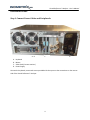
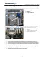
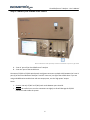
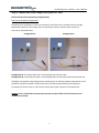
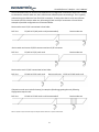
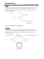
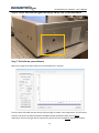
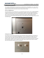
Virtual Reference™ Analyser
User's Manual
December 2014
Inometrix Inc.
35 Hemlock Way,
Grimsby, Ontario, Canada
L3M 0A8
Phone: 647-226-3715
Email: [email protected]
Web: www.inometrix.com
Virtual Reference™ Analyser – User's Manual
Contents
Introducing the Virtual Reference™ Analyser ............................................................................................... 3
Installation Guide .......................................................................................................................................... 4
Step 1: Connect Power Cables and Peripherals ........................................................................................ 4
Step 2: Connect Trigger & GPIB Cables .................................................................................................... 5
Step 3: Connect your tunable laser source ............................................................................................... 6
Step 4: Connect the device under test to the DUT Port ........................................................................... 7
Reflection based measurement configurations .................................................................................... 7
Transmission based measurement configurations ............................................................................... 9
Step 5: Turn on the instrument and start the software ......................................................................... 10
Step 6: Locate the detection gain switch(es) on the side of the instrument.......................................... 11
Step 7: Get to know your software ......................................................................................................... 11
Step 8: Scan the sample DUT provided ................................................................................................... 25
2
Virtual Reference™ Analyser – User's Manual
Introducing the Virtual Reference™ Analyser
Congratulations on your purchase of the Inometrix Virtual Reference™ Analyser. This manual
outlines the installation procedure as well as the use of the instrumentation software. After reading
this manual you should find that integrating the system with your tunable laser and using then
software is a relatively simple and straightforward process. As always if you do encounter any
difficulties we are always here to help, so please don’t hesitate to contact us.
Inometrix Inc.
35 Hemlock Way, Grimsby,
Ontario, Canada
L3M 0A8
Phone: 647-226-3715
Email: [email protected]
Web Site: www.inometrix.com
We hope you enjoy your new Virtual Reference™ Analyser!
3
Virtual Reference™ Analyser – User's Manual
Installation Guide
Step 1: Connect Power Cables and Peripherals
A B
A.
B.
C.
D.
C
D
Keyboard
Mouse
Video Card (Connect monitor)
Power Supply
Connect the keyboard, mouse and screen provided with the system to the connections on the reverse
side of the Virtual Reference™ Analyser.
4
Virtual Reference™ Analyser – User's Manual
Step 2: Connect Trigger & GPIB Cables
Connections on Virtual Reference™ Analyser
A. GPIB Port
B. Trigger in (SMB side)
Connections on tunable laser mainframe
(Agilent/Keysight 816XX A/B series)
C. GPIB port
D. Trigger out (BNC side of cable)
E. Remote interlock resistor
1. Connect a GPIB cable (provided) to the GPIB port of the Virtual Reference™ Analyser (A).
2. Connect the other side of the GPIB cable to the GPIB port on the tunable laser mainframe (C).
3. Connect the SMB side of the SMB-to-BNC cable (provided) to the SMB port labelled ‘Trigger in’
(B) on the Virtual Reference™ Analyser.
4. Connect the BNC side of the SMB-to-BNC cable (provided) to the port labelled ‘Trigger out’ (E)
on the tunable laser mainframe.
5. Ensure that the remote interlock resistor (D) is connected.
5
Virtual Reference™ Analyser – User's Manual
Step 3: Connect your tunable laser source
Note: tunable laser sold separately. Position and number of ports vary by model
A. ‘Laser in’ port of the Virtual Reference™ Analyser
B. ‘Laser out’ port of the tunable laser
Connect an FC/APC to FC/APC optical patch cord (green connectors on both sides) between the ‘Laser in’
port (A) of the Virtual Reference Analyser™ and the ‘Laser out’ port (B) of the tunable laser. If you are
using an 81600B series tunable laser with two output ports, use the ‘High power’ output.
Notes:
1. Caution: Use only FC/APC to FC/APC patch cords between ports A and B.
2. Caution: Be careful not to turn the connectors too tightly as this will damage the FC/APC
connector heads inside the system.
6
Virtual Reference™ Analyser – User's Manual
Step 4: Connect the device under test to the DUT Port
Reflection based measurement configurations
Fabry Perot (standard configuration)
The Fabry-Perot configuration is the most commonly used setup since it enables convenient single
ended measurements. In this setup, there are two ways to connect a device under test to the
instrument, illustrated below.
Configuration A
Configuration B
Configuration A: The device under test is connected directly to the DUT port
Configuration B: A sacrificial patchcord is connected between the DUT port and the device under test.
We highly reccommend using Configuration B exclusively for all reflection based measurements since it
protects the FC/APC connector inside the DUT port and reduces the possiblility that dirt/dust is
introduced into the DUT port. It is also easier to clean the FC/APC connector of the patch cord.
Caution: Be very careful not to overturn the connectors at the FC/APC to FC/PC interface as the
connectors may break.
7
Virtual Reference™ Analyser – User's Manual
The measurement setup in reflection will depend on the configuration of the device under test. In order
to characterize a device under test, there must be two reflection points surrounding it. This is typically
achieved using the reflections from flat FC/PC connectors. To ensure that there is only one reflection
from each side of the device under test, alternating FC/APC and FC/PC connectors are used. Some
examples of possible configurations are illustrated below.
Device under test is FC/PC connctorized on both sides:
DUT Port
FC/APC to FC/APC patch cord (recommended)
Device under test
Device under test has one FC/APC connector and one FC/PC connector:
DUT Port
FC/APC to FC/PC patch cord
Device under test
Device under test is FC/APC connctorized on both sides:
DUT Port
FC/APC to FC/PC patch cord
Device under test
FC/PC to FC/APC patch cord
If the device under test is a bulk element, for example a fiber Bragg grating then the following
configuration may be used:
DUT Port
FC/APC to FC/APC patch cord (recommended)
Note: An FC/APC to FC/PC connector may be used if the device under test is FC/APC connectorized.
8
Device under test
Virtual Reference™ Analyser – User's Manual
Michelson
The interference pattern produced by the Fabry perot setup is mathematically equivalent to the setup
below when the length of the coupler arms are balanced (equal). The following setup may be
advantageous over the Fabry perot setup if it is desireable to use mirrors (as illustrated bleow) to
increase the reflected power.
DUT Port
Coupler
Device under test
Transmission based measurement configurations
Mach-Zehnder
A transmission based measurement may be performed using a Mach-Zehnder configuration. In this
configuration two couplers with balanced (equal) arm lengths are used and the device under test is
placed in one of the paths. This configuration is useful when the device under test can only be
characterized in transmission.
Laser out (Tunable laser)
Balanced couplers
Device under test
9
DUT port (Virtual Reference™ Analyser)
Virtual Reference™ Analyser – User's Manual
Step 5: Turn on the instrument and start the software
Push the ‘Power’ button on the instrument
Click on the Virtual Reference™ Analyser shortcut
10
Virtual Reference™ Analyser – User's Manual
Step 6: Locate the detection gain switch(es) on the side of the instrument
Step 7: Get to know your software
Below is an image of the front panel of the Virtual Reference™ Analyser.
The front panel is divided into two sections (left and right) as shown in the image above. The left section
contains controls for the Scan Parameters and Measurement Parameters which are set before
experiment runtime. The right section contains the controls that are used during experiment runtime.
11
Virtual Reference™ Analyser – User's Manual
The Scan Parameters section sets the parameters
for controlling the tunable laser source. The
controls include the Start wavelength, Stop
wavelength and Output power. As there are
various tunable laser sources that may be used
with the system, the program does not prevent
out of bounds parameters from being input. The
user must ensure that the maximum/minimum
wavelengths and output power are within the
bounds of the particular tunable laser used.
The TLS port is the GPIB address of the tunable
laser mainframe used with the unit. By clicking on
the dropdown menu, the software automatically
searches for attached GPIB communication ports.
There is also a Refresh option in the dropdown
menu to search for new connections. Select the
GPIB address of the tunable laser.
The TLS mainframe is the mainframe of the
tunable laser source used with the unit. The unit is
compatible with legacy 816XA and new 816XB
tunable laser source mainframes from Keysight
(formerly Agilent Technologies).
The Channel selector is visible on systems with
more than one DUT port, depending on the model.
This image shows a model that is capable of
characterizing devices in the C/L band as well as
the O band.
12
Virtual Reference™ Analyser – User's Manual
The Measurement Parameters section sets the
pre-runtime experiment parameters.
The # of points is the desired number of measured
points in the dispersion curve. Note that this
number may be reduced for scans with noise.
In the Configuration dropdown menu select the
configuration used in Step 4.
Pressing the Scan button starts the tunable laser
scan and begins the measurement.
Pressing the Load button imports the raw scan
data (interference pattern) from a saved scan.
Pressing Quit exits the software.
The blue progress bar indicates the progress
through the measurement.
The Scan tab
13
Virtual Reference™ Analyser – User's Manual
After a scan has been completed, the Save Raw Scan button on the Scan tab saves a generic data file
(tab delimited text) of the raw interference pattern (intensity vs. wavelength). This file may be loaded
for analysis and dispersion characterization at a later time using the Load button.
If desired the raw interference pattern can be normalized and filtered by placing a check mark in the
Normalize scan and Apply FFT Filtering check boxes. By default, however, these boxes are left
unchecked as this step is usually not necessary.
The slider bar along the wavelength axis can be used to reduce the bandwidth of the scan range if
desired. To reduce the bandwidth simply click and drag the sliders. The slider on the left sets the
minimum wavelength and the slider on the right sets the maximum wavelength of the bandwidth
subset.
When finished click on the OK button to proceed to the next tab.
If the Normalize scan and Apply FFT Filtering check boxes are checked then the program automatically
advances to the Filter tab. If they are unchecked the program skips to the Balance/Fit tab.
The Filter tab (optional)
The Filter tab may be used to filter out frequency components in the raw scan. The top two plots show
the original scan and the result of FFT filtering. The bottom plot is an FFT of the original raw scan which
can be filtered using the slider tabs. Only half of this plot is unique (i.e. 0 to 0.5 contains the same
information as 1 to 0.5) so one side may be filtered out without any loss of information. This step is
typically employed to remove any low frequency components of the interference pattern.
14
Virtual Reference™ Analyser – User's Manual
When this step is complete, click on the OK button to advance to the next tab.
If the Normalize scan check box was checked on the Scan tab the software will automatically advance to
the Normalize tab. Otherwise it will advance to the Balance/Fit tab.
The Normalize tab
In the Normalize tab, use the Window size slider bar to vary the number of data points used in the
moving window that is used to scale the amplitude of the raw interference scan. This processing scales
the interference pattern so that the amplitude is normalized between -1 and 1 (arbitrary units) and
removes any noise in the amplitude of the interference pattern.
When this step is complete, click on the OK button to advance to the next tab.
15
Virtual Reference™ Analyser – User's Manual
The Balance/Fit tab
In this tab there are three sub tabs: Coarse Balance, Fine Balance and Fit.
With the Coarse Balance tab selected gradually increase the slider labelled Coarse Balance - Points in
FFT until there is a peak visible in the power spectrum. If there is more than one peak (measurement of
a DUT that is a cascade of elements (i.e. more than two reflection points) then change the number in the
Peak to reference box to select the appropriate cavity. For most measurements, however, there is
usually only one peak and this number is left at its default value of 1.
16
Virtual Reference™ Analyser – User's Manual
Once a peak is visible click on the Fine Balance sub tab.
By increasing the slider labelled Fine Balance - Sensitivity and using the arrows
, adjust the
length of the virtual reference so that the interference pattern may be 'Virtually Balanced' at a point
within the bandwidth of the scan range. The balance point is the location of the large peak/valley in the
amplitude modulation. Once the balancing has been achieved click on the Fit tab.
17
Virtual Reference™ Analyser – User's Manual
Vary the slider labelled Fit - Spline Parameter to filter out the high frequency component in the
interference pattern. The value should be high enough that the peaks and valleys have a good contrast
but low enough that there is only one point located for every peak (marked by X's). There is a wide
range of acceptable values for the Fit - Spline Parameter since we are only concerned with measuring
the phase of the interference and this does not depend on the amplitude of the interference pattern.
The length of the virtual reference path, Lv, may also be varied directly by placing a check mark in the
check box labelled Manually input Lv which allows the value of Lv to be input directly to the text box
beside Lv.
If a higher resolution is needed on the spline fit (plot on the Fit tab), place a check mark in the box
labelled Interpolate spline and in the text box labelled factor enter the number of times to interpolate
between spline points. This functionality is not typically required for most measurements though and
the default is not to use it.
When this step is complete, click on the OK button to advance to the next tab.
The Range tab
In this tab, the sweep range of the dispersion measurement can be set manually or automatically.
To set the sweep range automatically, place a check mark in the Automate Range Measurement check
box.
18
Virtual Reference™ Analyser – User's Manual
To set the sweep range manually, leave the Automate Range Measurement check box unchecked.
You may now use the sliders labelled Sensitivity to control the amount the virtual reference path length,
Lv, changes when the
arrows are pressed.
We may now set the spectral range of the dispersion measurement by choosing the maximum and
minimum value of the simulated virtual reference path, Lv.
In the top plot labelled Minimum Lv, press the
button to decrease the length of the virtual
reference path, Lv, and move the large peak to one side of the bandwidth (direction of movement in
the spectral domain depends on the sign of the dispersion of the device under test). To measure second
order dispersion, two peaks or two valleys are required on both sides of the largest peak/valley (point of
symmetry in the interference pattern) and the indicator
is bright blue when this is true.
In the top plot labelled Maximum Lv, press the
button to increase the length of the virtual
reference path, Lv, and move the large peak to one side of the bandwidth (direction of movement in the
spectral domain depends on the sign of the dispersion of the device under test). To measure second
order dispersion, two peaks or two valleys are required on both sides of the largest peak/valley (point of
symmetry in the interference pattern) and the indicator
is bright blue when this is true.
An alternative method for setting the Maximum Lv and Minimum Lv value is to input their values
directly to the text boxes
and
.
Below the two plots in the Range tab are a few additional controls.
For most measurements, these values can be left at their defaults. However, for users who wish to
optimize (further reduce the scatter) in the dispersion measurement results, these values may be
adjusted.
To use these controls, however, one must first understand how they affect the measurement of
dispersion from the interference pattern. Since second order dispersion is measured using the phase of
the interference pattern the locations of ALL the peaks and valleys of the interference pattern are
critical. The interference pattern, however, may include noise that can affect this measurement. These
controls set the parameters for filtering out this noise from the measurement process.
19
Virtual Reference™ Analyser – User's Manual
The first set of controls
sets the maximum allowable variation in the period of the interference pattern. For example, in the plot
below the deviation in the fringe period is the difference between Tp(n) and Tp(n+1). This deviation must
be less than the Maximum deviation in fringe period, Tmax (i.e. Tp(n) - Tp(n+1) < Tmax). Note: the
flexibility to vary the maximum deviation for the centre of the scan range and the edges of the scan
range will be discussed later.
When this condition is violated only the points up to the peak where the violation occurred are used in
the dispersion calculation. For example, if the interference plot has noise in it such that peaks are
erroneously located, as illustrated below
20
Virtual Reference™ Analyser – User's Manual
Since TL(4) - TL(3) < Tmax, the peaks/valleys to the left of 1520 nm are not included in the calculation of
second order dispersion. Also since TR(1) - TR(2) < Tmax the peaks/valleys to the right of 1615 nm are not
included in the calculation of second order dispersion. Therefore in this example only the peaks/valleys
between 1520 nm and 1615 nm are included in the dispersion calculation (9 peak/valley points).
The flexibility to vary the Maximum deviation in fringe period - centre of the scan range and Maximum
deviation in fringe period - edges of the scan range allows for variation in the maximum deviation
depending on where the large peak is during the sweep. For example, if the peak is near the centre of
the scan range then the period between visible points is large, as shown above. However, when the
large centre peak is located near the edges of the scan range, the period between visible points is
smaller, as shown below.
One may therefore reduce the tolerance for the Maximum deviation near the edges of the scan range in
comparison to that near the centre. The program then varies the tolerance linearly during the sweep.
In the previous example, the error in the peak locations limited the number of useable points in the
dispersion calculation to 9. The control
sets the
minimum number of peak or valley points required in order for a particular interference pattern to be
acceptable for use in the calculation of second order dispersion. The minimum number of peak/valley
points required for a measurement of second order dispersion to be possible is 5 since the large peak
and at least one peak and one valley on each side of the large peak are required. If the number of
useable points in a particular interference pattern is below the number specified in Minimum # of
peak/valley points in calculation, then that interference pattern is not used to calculate second order
dispersion and the value of Lv is incremented to see if the measurement can be made at a slightly
different wavelength. As a result, increasing this number results in higher accuracy but it leads to a
greater number of discarded points. It is important to note that the Minimum # of peak/valley points in
calculation must be less than the total number of peak/valley points in the scan range. Also note that
there are less peak/valley points when the large peak is at the centre of the scan range than when it is at
the edges of the scan range (where shorter period peaks/valleys are visible).
21
Virtual Reference™ Analyser – User's Manual
To accept interference patterns in which the large central peak has noise (multiple peaks/valleys located
on central peak) place a check mark in the check box
.
The control
determines if the algorithm that includes the
effect of third order dispersion in the calculation of second order dispersion is to be used. By default this
box is checked to include third order dispersion. When measuring a device with low third order
dispersion, however, this box may be unchecked to ignore the effect of third order dispersion. The
reason for using an algorithm that ignores third order dispersion is that it can help to reduce the scatter
in the dispersion plot (no noise from measuring third order dispersion).
When this step is complete, click on the OK button to advance to the next tab.
The Sweep tab
This tab is fully automated and shows the sweep from Lv minimum to Lv maximum set in the previous
tab.
22
Virtual Reference™ Analyser – User's Manual
The Results tab
This tab has three sub tabs to display the results of measurements of first and second order dispersion.
This includes Group Delay, Group Velocity Dispersion and Dispersion × Length. Sample plots are
illustrated in the following images.
23
Virtual Reference™ Analyser – User's Manual
The dispersion measurement results may be exported to a generic tab delimited text file that may be
opened in Matlab, Labview, Excel, Notepad or any text processing software. To export the results click
on
and save the file to the hard drive or a USB.
24
Virtual Reference™ Analyser – User's Manual
Step 8: Scan the sample DUT provided
In this step we use the system to measure a known sample to ensure everything is working as expected.
The sample provided with the Virtual Reference™ Analyser is a short length FC/PC to FC/PC
connectorized SMF28 patch cord.
Press the Scan button on the left side of the front panel.
You should immediately hear a click from the tunable laser and start to see the laser sweep between the
Start wavelength and the Stop wavelength at the set Output Power. Please consult the user's manual
of the particular tunable laser source used to determine the minimum and maximum
wavelength/output power. In order to allow for the use of multiple tunable lasers, we do not restrict
these values.
25
Virtual Reference™ Analyser – User's Manual
Bandwidth Range Adjustments:
The circulator provided with the standard system configuration has a bandwidth in the C and L band. If
you would like to characterize components outside this region please contact us for a circulator in your
region of interest and for instructions on how to install a new circulator.
Power Level Adjustments:
The optical power from the tunable laser may be adjusted programmatically from the Scan Parameters.
The gain of the detector built into the Virtual Reference™ Analyser may also be adjusted using the
controls at the side of the system. If the intensity measurements are 'clipped' (produce values greater
than 1 in the raw scan pattern) and power cannot be further reduced, reduce the detector gain.
Conversely if the power output of the tunable laser is maximized and the detected signal is low, increase
the detector gain.
Cleaning the connectors:
The connectors at the Laser IN and DUT ports may occasionally require cleaning. Use a screwdriver to
remove the screws not coloured green (highlighted in red in the image below). Carefully pull out the
connector and a short length of the fiber cable attached. Remove the connector to clean the fiber.
When cleaning is complete, reconnect the fiber and connector and reinstall the connectors to the front
panel. When the system is not in use please use the white caps provided with the system to prevent
dust from entering the optical ports of the front panel.
26