Download EAAT User Manual

EAAT User Manual
A guide how to use the Class Modeler
Dept of Industrial Information and Control Systems, KTH
November 2012
Content
EAAT User manual
4 1 Background
5 1.1 P2AMF: Predictive, Probabilistic Architecture Modeling Framework ............ 6 1.2 Probabilistic relational models (PRMs) ................................................. 10 1.3 The theory behind the tool ................................................................ 11 2 Specifying Theory in EAAT using the Class Modeler
2.1 2.2 14 Starting EAAT .................................................................................. 14 2.1.1 Getting familiar with the user interface .................................. 14 2.1.2 Menu bar ........................................................................... 15 2.1.3 Tool bar ............................................................................. 17 2.1.4 Info palette ........................................................................ 17 2.1.5 Model library ...................................................................... 19 2.1.6 View explorer ..................................................................... 19 Adding Classes ................................................................................ 19 2.2.1 Definition of the shape ......................................................... 20 2.2.2 Setting of icon/image .......................................................... 21 2.3 Adding Slots .................................................................................... 22 2.4 Adding Attributes ............................................................................. 25 2.4.1 Adding Discrete Attributes .................................................... 26 2.4.2 Adding Continuous Attributes ............................................... 26 2.4.3 Adding POCL Attributes ........................................................ 27 2.4.3.1 Adding POCL Operations and Invariants ................................. 28 2.5 2.4.4 Adding Self Reference.......................................................... 31 2.4.5 Edit Reference .................................................................... 31 Adding Attribute Relationships ........................................................... 32 2.5.1 Adding of internal Attribute Relationships ............................... 33 2.5.2 Setting of aggregation functions ........................................... 34 1.1.1.1 Setting of discrete aggregation functions ................................ 34 1.1.1.2 Setting of continuous aggregation functions............................ 35 3 Quick reference
36 4 Appendix
38 4.1 The structure of the CSV exports........................................................ 38 EAAT User manual
This document is a user manual for the Enterprise architecture Analysis
tool (EAAT). For more information about the tool project, please consider
http://www.ics.kth.se/eaat.
1
Background
The discipline of enterprise architecture advocates the use of models to
support decision-making on enterprise-wide information system issues. In
order to provide such support, enterprise architecture models should be
amenable to analyses of various properties, as e.g. the availability,
performance, interoperability, modifiability, and information security of
the modeled enterprise information systems. This manual describes a
software tool for such analyses. EAAT is an acronym for Enterprise
Architecture Analysis Tool and is a software system for modeling and
analysis of enterprises and their information systems.
The EAAT tool supports analysis of enterprise architecture models. The
tool guides the creaation of enterprise information system scenarios in the
form of enterprise architecture models and generates quantitative
assessments of the scenarios as they evolve. Assessments can be of
various quality attributes, such as information security, interoperability,
maintainability, performance, availability, usability, functional suitability,
and accuracy.
The EAAT tool consists of two parts, the Class modeler for defining the
underlying theory for the assessment and the Object modeler for modeling
enterprises and performing assessments. Theory definition is the activity
of identifying which phenomena are relevant for achieving the system
properties. For instance, security analysis requires modeling of
components such as firewalls, intrusion detection systems, anti malware
functions, access right definition and implementation, training of
personnel, the existence of business continuity plans and much more. In
the Class modeler, the structure and importance of these phenomena is
modeled. The Class modeler is thus mainly aimed to be used by
researchers. The second part of the tool is the Object modeler, which is
used to model concrete instances of system scenarios. The Object modeler
uses the theoretical framework developed in the Class modeler. The
Object modeler is mainly intended to be used by the industry. While this
manual focuses on the Class modeler, information about the Object
modeler
can
be
obtained
from
the
project
webpage
at
http://www.ics.kth.se
1.1 P2AMF:
Predictive,
Modeling Framework
Probabilistic
Architecture
The Object Constraint Language (OCL) is a formal language typically used to describe
constraints on UML models. These expressions typically specify invariant conditions
that must hold for the system being modeled, pre- and post conditions on operations
and methods, or queries over objects described in a model.
P2AMF, the Predictive, Probabilistic Architecture Modeling Framework is an
extension of OCL for probabilistic assessment and prediction of system qualities. The
main feature of P2AMF is its ability to express uncertainties of objects, relations and
attributes in the UML-models and perform probabilistic assessments incorporating
these uncertainties.
A typical usage of P2AMF would thus be to create a model for predicting, e.g., the
availability of a certain type of application. Assume the simple case where the
availability of the application is solely dependent on the availability of the redundant
servers executing the application; a P2AMF expression might look like this,
context Application :
attribute available : Boolean = s e l f . s e r v e r −> e x i s t s ( s : S e r v e r | s .
available)
This example demonstrates the similarity between P2AMF and OCL, since the
expression is not only a valid P2AMF expression, but also a valid OCL expression.
The fist line defines the context of the expression, namely the application. In the
second line, the attribute available is defined as a function of the availability of the
servers that execute it. In the example, it is sufficient that there exists one available
server for the application to be available.
In P2AMF, two kinds of uncertainty are introduced. Firstly, attributes may be
stochastic. When attributes are instantiated, their values are thus expressed as
probability distributions. For instance, the probability distribution of the instance
myServer.available might be
P(myServer . available )=0.99
The probability that a myServer instance is avail- able is thus 99%. For a normally
distributed attribute operatingCost of the type Real with a mean value of $ 3 500 and a
standard deviation of $ 200, the declaration would look like this,
P ( m y S e r v e r . o p e r a t i n g C o s t ) =N o r m a l ( 3 5 0 0 , 2 0 0 )
i.e. the operating costs of server is normally distributed with mean 3500 and standard
deviation 200.
Secondly, the existence of objects and relationships may be uncertain. It may, for
instance, be the case that we no longer know whether a specific server is still in service
or whether it has been retired. This is a case of object existence uncertainty.
Such uncertainty is specified using an existence at- tribute E that is mandatory for all
classes (here using the concept class in the regular object-oriented aspect of the word),
where the probability distribution of the instance myServer.E might be
P( myServer .E) =0.8
i.e. there is a 80% chance that the server still exists.
We may also be uncertain of whether myServer is still in the cluster servicing a
specific application, i.e. whether there is a connection between the server and the
application. Similarly, this relationship uncertainty is specified with an existence
attribute E on the relationships.
In this manual the reader will be confronted with P2AMF in three ways: (i) in the form
of metamodel attribute specifications, (ii) as metamodel invariants which constrain the
way in which the model may be constructed and (iii) as operations which are methods
that aid the specification of invariants and attributes.
An example metamodel attribute expression is shown below:
context UsageRelation
attribute self . ApplicationWeight : Real = getFunctionality
()/isAffected_1_inv .use_5_inv . Functionality
This is referring to the class UsageRelation in Figure 2 and specfies that
getFunctionality() operation should be utilized. The operation getFunctionality() is
specified as follows:
context UsageRelation
operation getFunctionality () : Real = self . isAffected_2 .
assigned_inv−>select (
oclIsKindOf ( ApplicationFunction ) ) . oclAsType ( ApplicationFunction ) .
Functionality−>sum()
where it says that getFunctionality() requires no input, and generates a Real as output
according to a statement.
An example invariant, noWriteAndRead, can be found below:
context InternalBehaviorElement invariant noWriteAndRead = not (
read_Function_inv−>e x i s t s ( do :
PassiveComponentSet | write_Function−> i n c l u d e s ( do ) ) )
This specifies that objects of the class InternalBehaviorElement from Figure 2 are not
allowed to both write and read the same data object.
A full exposition of the P2AMF language is beyond the scope Sufficient to say here
that the EAAT tool now implements P2AMF using the EMF-OCL plug-in to the
Eclipse Modeling Framework and has been employed to implement the metamodels of
this paper. The probabilistic aspects are implemented in a Monte Carlo fashion: In
every iteration, the stochastic P2AMF variables are instantiated with instance values
according to their respective distribution. This includes the existence of classes and
relationships, which are sometimes instantiated, sometimes not, depending on the
distribution. Then, each P2AMF statement is transformed into a proper OCL statement
and evaluated using the EMF-OCL interpreter. The final value returned by the model
when queried is a weighted mean of all the iterations.
BusinessService
InfrastructureService
ApplicationService
Functionality
Service
Availability
Response Time
EvidentialResponseTime
Workload
Arrival Frequency
Correction
Deterioration
EvidentialAvailability
0..*
0..1
Use_3
1
0..*
0..*
0..*
Use
Weight
Realize_1
WeightedWorkload
WeightedResponseTime
0..*
0..1
0..1
1
0..*
GateToGate_us
e (n)
Weight
rvice
Gate_use
Type
Execution Pattern
Availability
ResponseTime
0..*
1
rite_Service
Use_1
y
racy
Read_Function
Write_Function
0..*
0...1
UsageRelation
0..*
0..*
1
Regr.Coeff.TTF
GateToGate_realize
Weight
0..*
GateToGate_realize_bottom
Realize
Weight
WeightedWorkload
WeightedResponseTime
0..*
0..*
0..*
0..*
0..*
0...1
0..*
1
IsAffected_2
1
ApplicationComponent
Usage
Realize_3
1
InternalBehavioralElement (Function)
Availability
Evidential availability
Service Time
Arrival Frequency
Correction
Deterioration
Use_6
1
0..*
ActiveStructureElement
Assigned
0..*
0...1
Capacity
Availability
RoleComponentAssociation
PerceivedUsefulness
PerceivedEaseofUse
Use_7
epresentationSet
0..*
1
Role
Infrastructure Function
BusinessProcess
TaskFulfillment
1
Figure 1 P2AMF Example
ProcessServiceAssociation
Realize_2
0..*
nentSet
1
IsAffected_1
1
0..*
GateToGate_use_Bottom
GateToGate_realize_top
Gate_realize
Type
Execution Pattern
ResponseTime
Availability
Use_2
GateToGate_use_Top
Use_5
1
ApplicationFunction
Functionality
Node
Use_4
In this manual the historic name POCL will be used as a synonym to
P2AMF. The wording will be unified with the next major release of the tool
and its describing documentation.
1.2 Probabilistic relational models (PRMs)
A PRM Π specifies a probability distribution over all instantiations I of the
metamodel M. As a Bayesian network (Jensen 2001) it consists of a
qualitative dependency structure, and associated quantitative parameters.
The qualitative dependency structure is defined by associating attributes
X.A with a set of parents Pa(X.A). Each parent of X.A has the form X.τ.B
where B ∈ At(X.τ) and τ is either empty, a single reference slot φ or a
sequence
of
reference
slots
φ1,…,φk
such
that
for
all
i,
Range[φi]=Dom[φ(i+1)]. We call τ a slot chain. For example, the attribute
isDropped
of
class
Conversation
may
have
as
parent
Conversation.carrier.dropsMessage, meaning that the probability that a
certain conversation is dropped depends on the probability that message
passing systems that transmit the conversation drop messages. Note that
X.τ.B may reference a set of attributes rather than a single one. In these
cases, we let X.A depend probabilistically on an aggregated property over
those attributes. In this paper, we use the logical operations AND and OR
as aggregate functions. Considering the quantitative part of the PRM,
these aggregated properties are associated with a probability distribution
for the case when X.τ.B is an empty set in the architecture instantiation.
For example, if V(X.B)={True, False}, the aggregation function AND could
return X.B={True=0,False=1} if no parents are present in the
architecture instantiation.
Given a set of parents for an attribute, we can define a local probability
model by associating a conditional probability distribution with the
attribute,
P(X.A
|Pa(X.A)).
For
instance,
P(Conversation.isDropped=True|MessagePassingSystem.dropsMessage=F
alse)=10% specifies the probability that a conversation is dropped, given
the quality of the message passing system.
We can now define a PRM Π for a metamodel M as follows. For each class
X and each descriptive attribute A ∈ At(X), we have a set of parents
Pa(X.A), and a conditional probability distribution that represents PΠ
(X.A|Pa(X.A) ).
Given a relational skeleton σr (i.e. a metamodel instantiated without
attribute values), a PRM Π specifies a probability distribution over a set of
instantiations I consistent with σr (cf. Equation 1).
P(I σ r , Π ) = Π x∈σ r ( x )Π A∈At ( x ) P(x. A Pa(x. A))
P I σ! , Π = Π!∈!!
!
(Equation 1)
Π!∈!" ! P(x. A|Pa x. A )
Here σr(X) are the objects of each class as specified by the relational
skeleton σr. Hence, the attribute values can be inferred.
1.3 The theory behind the tool
Enterprise architecture models serve several purposes. Kurpjuweit and
Winter identify three distinct modeling purposes with regard to
information systems, viz. (i) documentation and communication, (ii)
analysis and explanation and (iii) design. The present article focuses on
the analysis and explanation (which is not to denigrate the usefulness of
the others). The reason is that analysis and explanation are closely related
to the notion of proper goals for enterprise architecture efforts. For
example, a business goal of decreasing downtime costs immediately leads
to an analysis interest in availability. This, in turn, defines the modeling
needs, e.g. the need to collect data on mean times to failure and repair.
In this sense, analysis is at the core of making rational decisions about
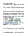
information systems. An analysis-centric process of enterprise architecture
is illustrated in Figure 2. In the first step, assessment scoping, the
problem is described in terms of one or a set of potential future scenarios
of the enterprise and in terms of the assessment criteria with its theory
(the PRM in the figure) to be used for scenario evaluation. In the second
step, the scenarios are detailed by a process of evidence collection,
resulting in a model (instantiated PRM, in the figure) for each scenario. In
the final step, analysis, quantitative values of the models' quality
attributes are calculated and the results are then visualized in the form of
e.g. enterprise architecture diagrams.
Figure 2 The process of enterprise architecture analysis with three main activities: (i)
setting the goal, (ii) collecting evidence and (iii) performing the analysis.
More concretely, assume that a decision maker in an electric utility is
contemplating changes related to the configuration of a substation. The
modification of a new access control policy would reduce the probability
that someone installs malware on a system and thereby reduce the risk
that this type of unwanted software is executed. The question for the
decision maker is whether this change is feasible or not. As mentioned in
the first step assessment scoping the decision maker identifies the
available decision alternatives, i.e. the enterprise information system
scenarios. In this step, the decision maker also needs to determine how
the scenario should be evaluated, i.e. the goal of the assessment. One
such goal could be to assess the security of an information system. Other
goals could be to assess the availability, interoperability or data quality of
the proposed to-be architecture. Often several quality attributes are
desirable goals. In this paper, without loss of generality, we simplify the
problem to the assessment of security of an electric power-station.
Information about the involved systems and their organizational context is
required for a good understanding of their data quality. For instance, it is
reasonable to believe that a firewall would increase the probability that
the system is secure. The availability of the firewall is thus one factor that
can affect the security and should therefore be recorded in the scenario
model. The decision maker needs to understand what information to
gather and also ensure that this information is indeed collected and
modeled. Overall, the effort aims to understand which attributes causally
influence the selected goal, viz. data quality. It might happen that the
attributes identified do not directly influence the goal. If so, an iterative
approach can be employed to identify further attributes causally affecting
the attributes found in the previous iteration. This iterative process
continues until all paths of attributes and causal relations between them,
have been broken down into attributes that are directly controllable for
the decision maker (cf. Figure 3).
Figure 3 Goal decomposition method.
In the second step collecting evidence the scenarios need to be detailed
with actual information to facilitate their analysis of them. Thus, once the
appropriate attributes have been set, the corresponding data is collected
throughout the organization. In particular, it should be noted here that the
collected data will not be perfect. Rather, it risks being incomplete and
uncertain. The tool handles this by allowing the user to enter the
credibility of the evidence depending on how large the deviations from the
true value are judged to be. In the third and final step, performing the
analysis, the decision alternatives are analyzed with respect to the goal
set e.g. security. The mathematical formalism plays a vital role in this
analysis. Using conditional probabilities and Bayes' rule, it is possible to
infer the values of the variables in the goal decomposition under different
architecture scenarios. By using the PRM formalism, the architecture
analysis accounts for two kinds of potential uncertainties: that of the
attribute values as well as that of the causal relations as such. Using this
analysis framework, the pros and cons of the scenarios can be weighted
against each other in order to determine which alternative ought to be
preferred.
2
Specifying Theory in EAAT using the
Class Modeler
The theory that should be used to perform analysis on is specified with the
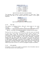
Class Modeler of the EAAT. This is generally performed by a researcher
whereas practitioners generally employ a predefined theory.
2.1 Starting EAAT
The EAAT is written in Java to enable platform independence and thus
requires Java JRE® to run (if missing, it can be downloaded at
http://www.java.com). For windows users the program is started by
executing the runClassModeler.bat
on MAC please use the ClassModeler application
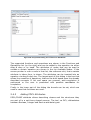
2.1.1
Getting familiar with the user interface
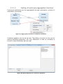
When starting the Class modeler the following window is displayed
Figure 4: The main window of the EAAT Class modeler with modeling pane, menu bar,
tool bar and status bar.
This view is dominated by the large modeling area, the white part of the
window. Apart from this there is the menu bar and the tool bar at the top
of the screen and the info palette at the right side. Following is a short
description of the menu choices and buttons in the tool bar, as well as the
info palette.
2.1.2
Menu bar
The menu offers several options. The file menu offers to create new class
models, open existing ones, save a model to file (including Save As …) to
adjust the used colors, to modify the type of an attribute, to connect a
class, to validate the modeled attribute relatiosn, to export to XML and
import to XML as well as to configure viewpoints. on the one hand and to
“Import From XML” on the other hand. Finally the tool can be closed from
the file menu too.
Figure 5: The File menu of the Class Modeler.
The views menu shows the views that are part of the currently opened
model.
The filter options allows specifying the visualization of the opened model.
Here it can be decided whether Attribute Relations, Class Relations,
Reference Labes, Role Labels, Attributes, Guide Lines, and OCL Operations
should be shown in the current view. Furthermore it can be selected if the
modeled classes should automatically adjust themselves to an underlying
visual grid.
Figure 6 The Filter options menu of the Class Modeler
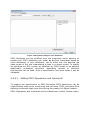
The POCL menu offers various POCL related tasks. The OCL-Code that has
been added to the model can be validated. For the Model the
corresponding Java code can be stored and finally the model can be
exported as an Ecore file.
Figure 7 The POCL options menu
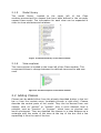
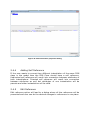
From the Mapping menu a mapping between an XSD (XML Schema) file
and the currently opened class model can be specified. This mapping can
be used to auto generate models.
Figure 8 The Mapping menu of the Class Modeler
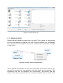
From the tool bars menu the different menus that the Class Modeler can
be shown.
Figure 9 The Tool bars menu of the Class Modeler
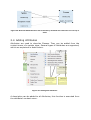
The template menu allows to define templates on Class level. These
templates can later on be reused during the creation of the object
diagrams.
Figure 10 The Template menu of the Class Modeler
2.1.3
Tool bar
The toolbar, as displayed below, allows for easy access to the most
common
functions
of
the
tool
Figure 11 : The toolbar of the EAAT Class modeller, containing the most common
commands.
Starting from the left there is a possibility to clear the scene and thereby
to start with a new model. The second function allows opening of an
existing model. These are followed by both save and save as …
functionality. Thereafter an option to take screenshots is offered. Followed
by zooming and the possibility to add views. Thereafter viewpoints,
defined upon the class model can be created. The next item allows to
configure the default behavior of the relations. Followed by a functionality
to add classes. Thereafter connections can be added. This is followed by
layout options offering alignment of the modeled classes and switching the
appearance from PRM to POCL adopted layout and back. Finally auto
refactoring can be turned on in order to propagate changes immediately.
2.1.4
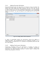
Info palette
Information on the current model is presented in the information area on
the left-hand side of the modeling pane.
Figure 12 : The Info Palette. It shows the information about selected object.
At the top of the info palette a satellite-view can be found. This presents
an overview of the model and is meant to help orienting and navigating
within large models. Below information panel can be found. Here a short
summary of the selected model-element is presented. In the lowest part
of the info palette several filters can be switched on or off. They are:
•
To show the connections on top of the classes
•
To show the relations between attributes
•
To show the relations between classes
•
To show the labels of the relationships
•
To show attributes
•
To show reference lines
•
To show PRM Classes as Shape Images
Figure 13: The Filter Panel.
2.1.5
Model library
The model library, located to the upper left of the Class
modeler,summarizes the classes that have been defined in the currently
opened class model. The information for each class can be expanded in
order to show attributes and relations.
Figure 14 The Model library of the Class modeler
2.1.6
View explorer
The view explorer is located to the lower left of the Class modeler. This
component allows to change between the defined views and to add new
ones.
Figure 15 The View explorer of the Class modeler
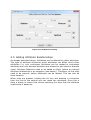
2.2 Adding Classes
Classes can be added either from the already described button in the tool
bar or from the context menu (available through a right-click). Classes
describe the central parts of the model. They can be derived from real
objects, such as “person” or “system”. Also a more abstract level is
possible, such as “function” or “process”, which have no physical real
world counterpart. They are depicted like classes in a class diagram as a
rectangle with the name of the class at the top of the box and a line
separating it from the rest of the box.
Classes can inherit properties from already existing classes, which can be
selected from their context menu, therefore the option “Set Superclass”
needs to be used.
Classes can be attributed (see description below). It is also possible to use
the “bring to front” function, so that they get visible even in complex
models. A description might be add from the context menu too.
Figure 16: Context menu for a Class. Set Super Class option will lead to following dialog.
Figure 17: Set Super Class Dialog.
2.2.1
Definition of the shape
Visual Configurations presents a dialog to the user to select Icon for PRM
Class as well as user will have the option to select Image shape
illustrating the functionality. So when user will select the “Show icon view”
in the filter panel then PRM class will be shown as selected shape image.
2.2.2
Setting of icon/image
After selecting the Visual Configurations option, a dialog will appear with
two tabs. The first tab (“Define Icon”) presents two options to user. First
user can select the icon from currently available icons library and second
option is to upload a new icon image.
The second tab (“Define Shape”) presents similar options for shape image.
The user can select shape images from the existing library and also has
the option to upload new shape images.
Figure 18: Define Shape Tab.
Figure 19: Define Icons Tab.
2.3 Adding Slots
Classes can be related to each other via slots. This is done by holding the
ctrl-key and drawing a relation from one Class to another one. Afterwards
those slots can be configured from their context menu (available through
a right-click).
Figure 20: Context menu for Slot Reference.
Three options are possible at first the properties of the slots can be set,
second the routing can be adjusted and third they can be deleted. The
properties that can be adjusted are multiplicities, role-names and the
name of the slots in general. If the routing is activated than a double-click
on a slot allows to either set or remove a control point (which is a fixed
point that is part of a slot and guides its visual appearance).
Figure 21: Slot Reference Properties.
It is also possible to add a slot from a certain Class to the same again.
This is done via the “Self-References” menu of the Class’ context menu.
Figure 22: Self Reference menu.
Either undirected or directed self-references can be used.
Figure 23: Undirected Self Reference.
The difference is that undirected self-references can be used to relate
attributes of an object of Class A to a second one and the other way
around, whereas directed one only allow relations from one object to
another one.
Slots determine which and how many relations are possible in the
instantiations (see below).
Figure 24: Directed Self Reference and Properties of Self Reference.
Figure 25: Directed Self Reference will be shown by directed self reference icon on top of
class.
2.4 Adding Attributes
Attributes are used to describe Classes. They can be added from the
context menu of a certain class. Several types of Attributes are supported,
which are explained in detail below.
Figure 26: Adding New Attribute.
A description can be added to all Attributes, this function is executed from
the attribute’s context menu.
2.4.1
Adding Discrete Attributes
Discrete Attributes allow the description of classes in terms of states. On
default the used states are high, medium, and low. But this can be
changed through the “Attribute Configurations” function. It is also possible
to use 1,2,3,4, and 5 or true and false. Additionally even customized
states are possible. This can be figured in the upper part of the Set CPM
dialog.
Figure 27: Setting CPM for Discrete Attribute.
In case of customized states the plus-button allows the adding of
additional states. The probabilities that the considered variable is in a
certain state (on a scale from 0 to 1) based on its potential parents can be
set in this dialog.
2.4.2
Adding Continuous Attributes
Continuous Attributes allow the description of classes in terms of
mathematical equations (which even can be probability distribution
functions). The “Set Attribute Properties” function opens a dialog that
allows these equations to be set.
Figure 28: Properties Dialog for Continuous Attributes.
The supported functions and operations are shown in the Functions and
Operations list (on the right) and can be added to the equation via either
drag & drop or by hand. The attributes of nodes that can be used to
creaate a certain equation are shown in the list Available Nodes. If the
mouse-pointer is over a node in that list, the reference slot, that a certain
attribute is taken from, is shown. The attributes can be inserted into an
equation via drag & drop too. The largest part of this dialog is the box that
allows the creaation of equations, that can be built based upon the already
described concepts. If ctrl and space are pressed, auto-completion is
performed or the user is presented with possible candidates for
completion.
Finally in the lower part of the dialog the bounds can be set, which are
used in case that functions are used.
2.4.3
Adding POCL Attributes
POCL/P2AMF attribute allows describing classes and the structures they
are part of in a set theory-based manner. The tool, as OCL, defrentiates
between Boolean, Integer and Real as attribute types.
Figure 29 Properties dialog for OCL Attributes
POCL-Attributes can be modified from the properties menu opening on
double-click. POCL-Attributes can either be derived (calculated based on
other attributes) or prior attributes, set by either the one defining the
class model or the one instantiating a class in a object model. To specify
an attribute the OCL syntax as specified by OMG needs to be applied.
Additionally probability functions, describing Normal or Bernoulli
distributions can be used. Once a specification has been made it can be
validated.
2.4.3.1
Adding POCL Operations and Invariants
To support the specification of POCL-Attributes POCL-Operations can be
used allowing code-reuse, structuring and recursion. POCL invariants allow
defining constraints that must hold during the creation of Object models.
POCL-Operations and Invariants can be added from a class’ context menu.
Figure 30 Adding POCL Operations and Invariants
Double-clicking an operation opens its properties dialog.
Figure 31 POCL Operations properties dialog
For each operation the input parameter and result can be defined through
a combination of:
Variable
LowerBound
UpperBuond
Single Value
1
1
Collection
0
-1
Array
0
Finite value e.g.
5, 10
Collection
Ordered
Unique
Set
False
true
OrderedSet
True
true
Sequence
True
false
Bag
false
false
Parameters can be added by right-clicking the name of the considered
operation
Double-clicking on an invariant shows a dialog allowing its specification.
Figure 32 POCL Invariants properties dialog
2.4.4
Adding Self Reference
If the user wants to connect two different instantiation of the same PRM
class in the model then the PRM Class should have a self reference.
Undirected self reference will result into connection between attributes of
both instantiations. Directed self reference will result into connection
between attributes as well but attributes of one instantiation will be
parents and other instantiation will be child.
2.4.5
Edit Reference
Edit reference option will lead to a dialog where all the references will be
presented and user can do the desired changes to references in one place.
Figure 33: Edit Reference Dialog.
2.5 Adding Attribute Relationships
As already described above, Attributes can be affected by other attributes.
The type of attribute influences which attributes can affect which other
attributes (i.e. only continuous Attributes can be related to continuous
attributes and only discrete attributes are allowed to get linked to discrete
ones). Attribute Relations need to be based on Slots (where an internal
Attribute relationship is an exception (see below)). Therefore, at first slots
need to be present, before Attributes can be related. This can also be
done iterative.
When slots are present, holding the ctrl key and drawing a connection
from the first to the second one can relate two attributes. Once this is
done a dialog is shown that allows selecting the slots that the attribute
relationship is based on.
Figure 34: Path Determination Dialog for Attributes Relation.
In this dialogue the user selects which slots the attribute relationship is
associated with. When the target is reached green icons symbolize that
the relation is valid. Yellow arrows allow reverts the last action.
Attributes need to be related in order to serve as input to each other. This
means that in case that discrete Attributes are used, the states of the
Attributes only appear, when the Attributes have been related previously.
For continuous variables it means that before Attributes can be used in
equations they need to be related.
2.5.1
Adding of internal Attribute Relationships
Attributes of the same class might also be related without the usage of
slots, so that they are related on each instantiation of that Class
automatically. The relation is creaated as all others are. In the dialog that
is presented the box “Internal Reference” needs to be checked afterwards.
2.5.2
Setting of aggregation functions
Aggregation functions describe how several instances of the same
Attribute are combined during the calculation. The usage of aggregation
functions is needed as during the theory-modeling the amount of linked
instances is unclear (i.e. aggregation functions make the theory prepared
to handle dynamic aspects of the instantiations).
As aggregation functions are used to handle dynamic aspects they are
only used when several nodes need to be aggregated. This means that in
case only one parent is allowed (through multiplicities), no aggregation is
necessary. If the number of parents is unclear (* multiplicity) they are
utilized. To overcome the fact that there also might be zero parents
modeled a “Default CPT” can be set (the option is available in an Attribute
Relationship’s context menu), which serves as alternative input in case of
nothing else being available.
Figure 35: Default CPT Dialog for Attributes Relation.
1.1.1.1
Setting of discrete aggregation functions
Discrete attributes can be aggregated through Max, Min or Average CPTs.
The states of the default CPT match the states of the attribute they are
supposed to replace.
Figure 36: Aggregation Functions for Attributes Relation.
1.1.1.2
Setting of continuous aggregation functions
Continuous attributes can be aggregated through summation, product or
calculation of average.
Figure 37: Aggregation function for continuous attributes.
A default equation can be set as well. The dialog is similar to the one for
setting Attribute properties; the only difference is that no variables in
terms of other Attributes can be used.
Figure 38: Default Equation for continuous Attribute.
3
Quick reference
Class modeler. The Class modeler is the part of the EAAT where the
underlying theory for enterprise architecture assessments is specified.
Here, the concepts and relationships relevant for different kinds of
analysis is defined, thus enabling the users of the Object modeler to
perform advanced assessments in an automatic, easy fashion.
Bayesian network. A Bayesian network is a probabilistic graphical model
that represents a set of variables and their probabilistic dependencies.
Bayesian networks combine a rigorous mathematical handling of
uncertainty with a graphical and intuitive depiction of causal relationships
between different phenomena. Bayesian calculations are at the heart of
enterprise architecture analysis using the EAAT.
Class. A class is a category that modeled elements can belong to. When a
modeled element in a object model belongs to a class, it means that it has
assigned the attributes associated with that class as defined in the class
model. For instance, the class “system” might contain attributes such as
“information security” or “performance” whereas for the class “process”
might have attributes such as “efficiency” or “cycle time”.
Credibility. Different data have different credibility, depending on
whether the source is reliable, whether it is recently collected etc. When
conducting enterprise architecture analyses, it is of greaat importance that
models and decisions are not based on flawed or biased data. By requiring
the user to specify the credibility of the data used, the EAAT tool manages
this aspect of data collection.
Enterprise architecture. The discipline of advocates the use of models
to support decision-making on enterprise-wide information system issues.
By analyzing the relevant data in a structured, and preferably
quantitative, way, better management decisions can be made.
Evidence. Evidence is the data about real world circumstances, collected
for the purpose of enterprise architecture analysis. Such evidence is never
certain, but rather has a level of credibility that can be taken into account
when performing the analysis. The EAAT Objecy modeler allows the user
to provide evidence(s) regarding the states of every attribute, including
the more complex ones, should such knowledge be available.
Model. A model is a simplified representation of the real world,
specifically designed to capture the aspects relevant for a certain purpose,
and leave other aspects out. Enterprise architecture models try to
incorporate those feaatures relevant to decision making on enterprisewide information system issues. The EAAT tool distinguishes two types of
models: the class model that speaks of general relationships such as
availability and maintenance organizations, and object models that speak
of particular companies and situations, such as the availability of system X
on company Y. The idea is that the class models are provided by
researchers as support for the industry that deals primarily with object
models.
Model Library Tree. Represents the model as a whole and describes the
hierarchy of different objects in the model.
Object. An object is a modeling concept, usually referring to something
that is part of the real world. Enterprise, CRM system, computer, and
project team are all examples of possible objects. Objects have attributes
and belong to classes
Object modeler. The Object modeler is used to model instances of
system scenarios. The Object modeler uses the theoretical framework
developed in the Class modeler to direct and enable complicated
enterprise architecture analyses, without a need for the user to be a
theoretical expert. The Object modeler is mainly intended to be used by
enterprise architects in the industry.
Relationship. Relationships describe how different classes relate to each
other. Observable regularities in the real world are modeled as
relationships, such as when the “reliability of components decreases, the
maintenance costs increase”. Relationships based on research are created
in the Class modeler, where they serve as templates for analyses in the
Object modeler.
View. Represents sub set of model designed to have specialized
visualizations. There can be two types of views. First type is normal views
which are creaated by user to have some specific visualization and second
type views are called analysis view which comes into being to show
analysis for a specific attribute.
4
Appendix
4.1 The structure of the CSV exports
The following schema describes how the resulting excel files are
structured:
Name
Meaning
Object-name
The name of the object
Attribute-name
The name of the attribute
Class
The class that the object is an instance of
Attribute-type
The type of the attribute (which right now is either
discrete or continuous)
Continuousvalue
If the attribute is continuous than the continuous value
(after calculation)
State1-name
If the attribute is discrete than the name of the fist state
State1-value
If the attribute is discrete than the probability for that
state (after calculation)
...
If the attribute is discrete than the name of the next
state
...
If the attribute is discrete than the probability for that
state (after calculation)
Staten-name
If the attribute is discrete than the name of the nth state
Staten-value
If the attribute is discrete than the probability for tha
state (after calculation)