1
TECHNICAL REPORTS
25
CO2
CH4
CO
Greenhouse
The WRF Greenhouse Gas Model
(WRF-GHG)
by
Veronika Beck
ISSN 1615-7400
Gas Model
W
F
R
Technical Reports - Max-Planck-Institut für Biogeochemie 25, 2011
Max-Planck-Institut für Biogeochemie
P.O.Box 10 01 64
07701 Jena/Germany
phone: +49 3641 576-0
fax: + 49 3641 577300
http://www.bgc-jena.mpg.de
The WRF Greenhouse Gas Model
(WRF-GHG)
written by
1
Veronika Beck , Thomas Koch , Roberto Kretschmer1 , Julia Marshall1 ,
Ravan Ahmadov2,3 , Christoph Gerbig1 , Dhanyalekshmi Pillai1 , and
Martin Heimann1
1
1
Max Planck Institute for Biogeochemistry, Jena, Germany
NOAA Earth System Research Laboratory, Boulder, Colorado, USA
3 also at: Cooperative Institute for Research in Environmental Sciences, University of
Colorado, Boulder, USA
2
Contents
1 Overview
1
2 The WRF Greenhouse Gas Model (WRF-GHG)
2.1 Description of WRF-GHG . . . . . . . . . . . . . . . . .
2.1.1 Development history of WRF-GHG . . . . . . .
2.1.2 Tracer transport within WRF-GHG . . . . . . .
2.1.3 Description of the code structure of WRF-GHG .
2.2 Initial and boundary conditions . . . . . . . . . . . . . .
2.3 CO2 , CH4 , and CO fluxes in WRF-GHG . . . . . . . . .
2.3.1 Online calculated fluxes . . . . . . . . . . . . . .
2.3.2 External flux data sets . . . . . . . . . . . . . . .
.
.
.
.
.
.
.
.
.
.
.
.
.
.
.
.
.
.
.
.
.
.
.
.
.
.
.
.
.
.
.
.
.
.
.
.
.
.
.
.
.
.
.
.
.
.
.
.
.
.
.
.
.
.
.
.
.
.
.
.
.
.
.
.
.
.
.
.
.
.
.
.
3 WRF-GHG Preprocessors
3.1 VPRM-Preprocessor . . . . . . . . . . . . . . . . . . . . . . . . . . . . .
3.1.1 Description of the VPRM-Preprocessor . . . . . . . . . . . . . .
3.1.2 Installation, Configuration and usage of the VPRM-Preprocessor
3.2 Biomass burning preprocessor:
Prep− chem− sources . . . . . . . . . . . . . . . . . . . . . . . . . . . . .
3.2.1 Description of the preprocessor . . . . . . . . . . . . . . . . . . .
3.2.2 Running the preprocessor . . . . . . . . . . . . . . . . . . . . . .
3.3 Walter wetland model . . . . . . . . . . . . . . . . . . . . . . . . . . . .
.
.
.
.
.
.
.
.
.
.
.
.
.
.
.
.
3
3
3
4
5
10
12
12
19
25
. . 25
. . 25
. . 26
.
.
.
.
.
.
.
.
29
29
29
32
4 How to run WRF-GHG
35
4.1 Steps to run WRF-GHG . . . . . . . . . . . . . . . . . . . . . . . . . . . . . 35
4.2 Namelist settings . . . . . . . . . . . . . . . . . . . . . . . . . . . . . . . . . 36
4.3 Matlab script . . . . . . . . . . . . . . . . . . . . . . . . . . . . . . . . . . . 38
A Coupling the GHG model to a new WRF release
41
B Figures
47
C Model Organizing Software System (MOSS)
53
C.1 Steps to start a WRF-GHG simulation with MOSS . . . . . . . . . . . . . . 53
D Running WRF-GHG without Matlab
59
List of figures . . . . . . . . . . . . . . . . . . . . . . . . . . . . . . . . . . . . . . 69
Bibliography . . . . . . . . . . . . . . . . . . . . . . . . . . . . . . . . . . . . . . 71
i
Technical Report No. 25: The WRF Greenhouse Gas Model
IMPORTANT NOTE: CODE ACCESS AND COPYING
The WRF-GHG code is copyrighted. This User’s Guide is the only documentation
provided with this release of WRF-GHG. You may NOT make copies of any part of the
code for distribution to any other person or group.
The WRF-GHG source code is distributed for free on request. Please email to Veronika
Beck ([email protected]), Thomas Koch ([email protected]), or Christoph
Gerbig ([email protected]) to obtain registration and access information. Afterwards, the source code can be downloaded from the following webpage http://www.
bgc-jena.mpg.de/bgc-systems/index.shtml/ under the button “Download”.
If you use WRF-GHG in your research:
• We request that you include the following acknowledgement in the relevant manuscripts:
“WRF-GHG is provided by the Max Planck Institute for Biogeochemistry, Germany.
MPI assumes no responsibility for the proper use of WRF-GHG by others.”
• Please reference WRF-GHG:
Beck, V., T. Koch, R. Kretschmer, J. Marshall, R. Ahmadov, C. Gerbig, D. Pillai,
and M. Heimann, (2011): The WRF Greenhouse Gas Model (WRF-GHG). Technical
Report No. 25, Max Planck Institute for Biogeochemistry, Jena, Germany.
If you have made any significant modifications to the code, please mention them in
your manuscript.
We are interested to get reports from users about new applications of WRF-GHG, including any problems that come up. If you have questions about the code, appropriate
model applications, possible programming errors, etc., please read this entire guide first,
and then feel free to contact:
Veronika Beck ([email protected]) or Christoph Gerbig ([email protected])
iii
Chapter 1
Overview
In the context of global warming and climate change, carbon dioxide (CO2 ) and methane
(CH4 ), the two most important greenhouse gases, gain more and more attention. In addition to atmospheric observations of greenhouse gases (and additionally, carbon monoxide
(CO) used as a tracer for CO2 and CH4 ) and a required thorough understanding of the
processes emitting and consuming CO2 and CH4 , powerful models are indispensable to
predict possible impacts of climate change. To achieve this goal, transport simulations
of greenhouse gases in the atmosphere at high resolution are essential. Addressing this
need, the WRF Greenhouse Gas model was developed to allow for passive tracer transport
simulations of CO2 , CH4 , and CO. Several flux models and emission inventories are used
for an estimation of the emission and consumption fluxes of CO2 , CH4 , and CO. These
flux models are either coupled online, i.e. their code is implemented into the WRF-GHG
code or are operated as preprocessors for WRF-GHG to calculate fluxes for the different source and sink processes for CO2 (autotrophic respiration, photosynthesis, biomass
burning, other anthropogenic emissions, termites, ocean sources), CH4 (wetlands, biomass
burning, other anthropogenic emissions, termites, soil uptake) and CO (biomass burning,
other anthropogenic emissions).
The main intention of this technical report is to serve as a user guide for WRF-GHG
users and developers. The technical report is organized as followed:
The development history of the WRF-GHG code and a detailed description of the
WRF-GHG structure is given in Chapter 2. The usage of initial and boundary conditions
for the greenhouse gas tracer and the depiction of the different flux models used within
WRF-GHG is also found in this chapter.
Chapter 3 focuses on the preprocessors of WRF-GHG. The VPRM-Preprocessor, a
biomass burning preprocessor and the Walter wetland model are described in this chapter with the main focus on the installation, configuration and running of the preprocessors.
Namelist settings, compilation, a list of steps how to run WRF-GHG, and a description
of the matlab script used to read in CO2 , CH4 , and CO flux fields as well as initial and
boundary conditions into the WRF model can be found in Chapter 4.
1
Technical Report No. 25: The WRF Greenhouse Gas Model
Everything required to update WRF-GHG to a more recent WRF version (currently
WRFV3.2 is used) is described in Appendix A. Appendix B illustrates some results of
WRF simulations using WRF-GHG in the Amazon region. In Appendix C, the use of the
Model Organizing Software System (MOSS) for automatized simulations of WRF-GHG
is explained. The use of open source NCO commands in place of matlab scripts for the
manipulation of flux fields and lateral boundary conditions is described in Appendix D.
2
Chapter 2
The WRF Greenhouse Gas Model
(WRF-GHG)
The WRF Greehouse Gas model (WRF-GHG) is an augmentation of the coupled Weather
Reasearch and Forecasting model (WRF) to the Vegetation Photosynthesis and Respiration model (VPRM), WRF-VPRM, which is described in detail in Ahmadov et al. [2007]
(WRF-VPRM). The main objective of WRF-VPRM is to simulate high resolution passive tracer transport of carbon dioxide (CO2 ). WRF-GHG is an extension of WRF-VPRM
allowing for passive tracer transport not only for CO2 , but also for methane (CH4 ) and carbon monoxide (CO). A further advantage of both WRF-GHG and WRF-VPRM is that
initial and boundary conditions can be derived from three-dimensional fields of global
simulations of CO2 , CH4 and CO, e.g. resulting from fluxes optimized by atmospheric
inversions on a global scale. CO2 , CH4 and CO fluxes from different source and sink
processes are either calculated “online” (the flux model is implemented in the WRF-GHG
code) or “offline” (an external e.g. process-based bottom-up model is used to calculate
the fluxes which are then transported inside WRF-GHG).
Chapter 1 first gives a description of WRF-GHG with its newly introduced modules
and routines, followed by the set-up for the initial and boundary conditions. Finally, a
short illustration of all flux models and datasets used for the calculation of CO2 , CH4 ,
and CO fluxes concludes this chapter.
2.1
2.1.1
Description of WRF-GHG
Development history of WRF-GHG
The main motivation for developing WRF-GHG was its application to perform regional
simulations of CO2 , CH4 , and CO transport in the atmosphere over the Amazon basin
during the BARCA (Balanço Atmosférico Regional de Carbona na Amazônia) project.
The coupling of the GHG model to the WRF model started with WRF version WRFV3.1.1
and was then upgraded to WRF version V3.2. Meanwhile, WRF-GHG has been tested
for Siberia and the Amazon region (both using WRF-GHG based on WRFV3.2 version)
and Europe (still as the WRF-VPRM based on WRFV3.0.1 version performing only CO2
simulations) with different the physics options of the WRF model shown in Table 2.1.
3
Technical Report No. 25: The WRF Greenhouse Gas Model
Physics schemes
Radiation
Microphysics
Cumulus parametrization
PBL parametrization
Surface layer
Land surface model
Physics schemes
Radiation
Microphysics
Cumulus parametrization
PBL parametrization
Surface layer
Land surface model
Options Europe/Siberia
rrtm scheme (longwave) Dudhia scheme (shortwave)
WSM 5-class scheme
Kain-Fritsch (new Eta) scheme
YSU or MYJ scheme
Monin-Obukhov scheme
NOAH-LSM
Options Amazon
RRTMG long and short wave
WSM 5-class scheme
Grell-Devenyi and Grell3
MYJ (Eta) TKE scheme
Monin-Obukhov (Janjic Eta) scheme
NOAH-LSM
Table 2.1: Physics options of WRF-GHG used for Europe and Siberia and the Amazon
region.
2.1.2
Tracer transport within WRF-GHG
The WRF model (ARW core) uses fully compressible, non-hydrostatic Eulerian equations on an Arakawa C-staggered grid with conservation of mass, momentum, entropy,
and scalars [Skamarock et al., 2008]. Tracers are transported online in a passive way,
i.e. without any chemical reactions within the framework of the GHG− TRACER package
with chemistry option 98 (chem− opt == 98) in the namelist.input file (see Sec. 4.2 for
details). Therefore all chemical mechanisms besides vertical mixing are turned off if the
tracer transport option is used [Ahmadov et al., 2007]. Online tracer transport implies
that transport is performed simultaneously with the meteorological variables at each time
step [Ahmadov et al., 2007]. Emissions are added at each time step to the tracer concentration in the lowest model layer. The tracers undergo the advection, boundary layer, and
convective mixing as the chemical species. Additionally, from WRFV3.1.1 onwards an option for subgrid convective transport of chemical species has been implemented [Peckham
et al., 2009].
In WRF-Chem Version 3.2 a tracer option has already been implemented [Peckham et
al., 2009], but here the separate GHG− TRACER package is used to allow for online calculation
of CO2 and CH4 fluxes inside the WRF-Chem model [Grell et al., 2005]. Additionally,
other features such as the coupled plumerise mechanism for biomass burning emissions
[Grell et al., 2010] are available in the GHG− TRACER package which are not available with
the standard WRF-Chem tracer option and emissions are handled differently, e.g. no dry
deposition.
4
Technical Report No. 25: The WRF Greenhouse Gas Model
2.1.3
Description of the code structure of WRF-GHG
Basically, the necessary modifications to the “usual” WRF code for WRF-GHG consist of four additional modules which are added to the WRF-Chem source code and
some additional required minor modifications to the WRF-Chem source code itself. The
new modules consist of a separate registry file (registry.ghg), where all the additional
tracer and flux variables used inside WRF-GHG are defined, which is included in the
usual WRF-Chem registry (Registry.EM− CHEM) and the greenhouse gas module itself
(module− greenhouse− gases.F) which contains two main parts, the connection of the
emissions (fluxes) to the atmospheric concentrations (tracer) and the online calculation
of several CO2 and CH4 flux fields. Further on, the subroutines for converting fluxes
into atmospheric concentrations and adding them to the corresponding tracer variable are
located in module− add− emissions.F. For biomass burning fluxes and the corresponding
tracer, the plumerise model, also part of the standard WRF-Chem [Grell et al., 2010], was
modified and adapted to the needs of WRF-GHG and can now be used as an additional
option (module− plumerise− ghg.F). The subroutine for the greenhouse gas module contains all calls to subroutines for the calculation of online fluxes and the addition of tracer
concentrations. It, in turn, is called by the chem− driver.F routine in the <WRFV3/chem>
directory if chem− opt == 98 is set in the namelist.input file.
In the following subsections the four additional modules (registry.ghg, module− add
emissions.F,module
−
− greenhouse− gases.F, and module− plumerise− ghg.F) are explained in more detail.
registry.ghg
The registry.ghg file is located in the WRF-GHG code in the directory <WRFV3/
Registry> and included in the main registry of the WRF-Chem model (Registry.EM
− CHEM). All additional variables for tracers and fluxes used by WRF-GHG, variables
needed for the online calculation of fluxes, and all the WRF-GHG-specific namelist options are defined here. For more detailed information on the system of defining variables
in the WRF registry see the WRF registry description of Michalakes and Schaffer [2004].
All variables defined in registry.ghg are global variables and the empty arrays are created in the wrfinput (and additionally also in the wrfbdy file) if it is specified in the
namelist.input file that lateral boundary conditions are requested (for all tracers, see
namelist option have− bcs− chem = .true. in Sec. 4.2). If it was defined in registry.ghg,
the variables are also written to the wrfoutput file.
All tracers are defined as four-dimensional chem arrays in the registry.ghg file. The
notation is CO2− 1, ...,CO2− 6 and CO2− B for CO2 , CH4− 1, ...,CH4− 7 and CH4− B for
CH4 , and COT− 1, ...,COT− 3 and COT− B for CO. The unit of the tracer is [kg/kg].
An overview on the assignment of the single tracer variables to different source and sink
processes of CO2 , CH4 , and CO is illustrated in Table 2.2.
Additionally, all flux variables representing fluxes of different processes emitting or
consuming CO2 , CH4 and CO are defined in registry.ghg. Table 2.3 illustrates a full
overview of all fluxes (units in [kg/m2 s]) defined in registry.ghg. The flux variable
5
Technical Report No. 25: The WRF Greenhouse Gas Model
Variable (chem)
CO2− 1
CO2− 2
CO2− 3
CO2− 4
CO2− 5
CO2− 6
CO2− B
CH4− 1
CH4− 2
CH4− 3
CH4− 4
CH4− 5
CH4− 6
CH4− 7
CH4− B
COT− 1
COT− 2
COT− 3
COT− B
Tracer
total atmospheric CO2 concentration
changes in CO2 concentration from biogenic activity
changes in CO2 concentration from anthropogenic emissions
changes in CO2 concentration from biomass burning
changes in CO2 concentration from termites
changes in CO2 concentration from ocean fluxes
atmospheric CO2 background concentration
total atmospheric CH4 concentration
changes in CH4 concentration from wetland emissions
changes in CH4 concentration from anthropogenic emissions
changes in CH4 concentration from biomass burning
changes in CH4 concentration from termite emissions
changes in CH4 concentration from soil uptake
changes in CH4 concentration from vegetation
atmospheric CH4 background concentration
total atmospheric CO concentration
changes in CO concentration from biomass burning
changes in CO concentration from anthropogenic emissions
atmospheric CO background concentration
Table 2.2: Overview of all tracer variables defined in the registry.ghg file
also defines the time dimension of the external flux which can be either hourly (30 time
steps per simulation day) or daily (one time step per day). In case the external fluxes are
on different time resolutions, the time dimension of the flux variable can be adjusted in
registry.ghg. The time resolution of internal calculated fluxes depends on the time step
of the model and the output history time step that can be specified in the namelist.input
file. A detailed description of the online flux calculation and the models coupled online to
WRF-GHG follows in Sec. 2.1.3.
Furthermore, all the namelist options that had been established for the WRF-GHG
and that are new in the namelist.input file are defined here. The last line of the
registry.ghg file shows how the WRF-GHG is defined: It is defined as chemistry option
98 (chem− opt=98) and the package is called GHG− TRACER.
module− add− emissions.F
module− add− emissions.F contains all subroutines for adding the emissions of CO2 , CH4 ,
and CO calculated per time step to the corresponding atmospheric concentrations (see
Table 2.2). Emissions are usually added to the atmospheric concentrations at the first
model layer. All subroutines in this module are called from module− greenhouse− gases.F,
described in more detail in this section below.
module− add− emissions.F consists of the four subroutines co2− surface− source− add,
co2− surface− source− ad2, add− emis− anthro− ghg, and add− emis− burn− ghg. All these
6
Technical Report No. 25: The WRF Greenhouse Gas Model
Variable (chem− source)
CO2
fl− bio1
fl− oce
fl− ant1
fl− antco2
fl− bbco2
bb− co2
GEE
RESP
co2− term
CH4
fl− wet
fl− ant4
fl− antch4
fl− bbch4
bb− ch4
fl− term
fl− soilu
fl− veg
ch4− emiss
ch4− term
ch4− soil
ch4− veg
CO
fl− ant5
fl− antco
fl− bbco
bb− co
Flux component
Time Dimension
ext. biospheric
ext. ocean
ext. anthropogenic
ext. anthropogenic
ext. biomass burning
3d int. biomass burning
int. Gros-Ecosystem-Exchange
int. biospheric respiration
int. termite emission
hourly [30]
hourly [30]
daily [1]
hourly [30]
daily [1]
WRF timestep
WRF timestep
WRF timestep
WRF timestep
ext. wetland
ext. anthropogenic
ext. anthropogenic
ext. biomass burning
3d int. biomass burning
ext. termite emission
ext. soil uptake
ext. vegetation
int. wetland
int. termite emission
int. soil uptake
int. vegetation
hourly [30]
daily [1]
hourly [30]
daily [1]
WRF timestep
daily [1]
hourly [30]
hourly [30]
WRF timestep
WRF timestep
WRF timestep
WRF timestep
ext. anthropogenic
ext. anthropogenic
ext. biomass burning
3d int. biomass burning
daily [1]
hourly [30]
daily [1]
WRF timestep
Table 2.3: Overview over all flux variables used in the WRF-GHG model that are defined
in the registry.ghg file. “Ext.” implies offline/external calculation of fluxes or use of
emission inventories and “int.” online calculation of fluxes and internal variables. The
time step of the external fluxes can be either daily or hourly. For the internal fluxes the
time step of calculation depends on the time step of the WRF model.
subroutines follow the same principle in adding fluxes to atmospheric concentrations. The
two-dimensional flux variable chem− source(i,j) (for values see Table 2.3) is multiplied
by a conversion factor (conv− rho(i,k,j)) and added to the first layer of the threedimensional tracer variable chem(i,k,j) (for values see Table 2.2). If the plumerise
mechanism is used, biomass burning emissions are added at all vertical layers. The addition of fluxes to the concentrations is illustrated in the following formulas using the
variable names of the WRF-GHG source code:
chem(i, 1, j) = chem− source(i, j)
2
kg
sm
×
conv
rho(i,
1,
j)
−
m2 s
kg
(2.1)
7
Technical Report No. 25: The WRF Greenhouse Gas Model
with
conv− rho(i, 1, j) =
1
kg
rho(i, 1, j)[ m
3]
×
dt[s]
.
dz8(i, 1, j)[m]
(2.2)
Here rho(i, 1, j) denotes the air density in the first model layer, dt the time step of the
model and dz8(i, 1, j) the thickness of the first model layer in [m].
Subroutine co2− surfac− source− add is used to add emissions without any specific
features using eq. (2.1) to the first model layer. If biomass burning emissions are added
into the first model layer, and additionally a diurnal cycle peaking at 18 UTC (14:00 local
time) for biomass burning emissions [Prins et al., 1998] is applied (multiplication factor to
emissions) subroutine co2− surfac− source− ad2 needs to be used. If the EDGAR emission
inventory is used with an hourly time step containing a diurnal cycle (details in Sec. 2.3.2),
but constant for each weekday, the subroutine add− emis− anthro− ghg is applied. This
multiplies the emissions with a weekly cycle accounting for less traffic on the weekends
compared to weekdays [Alonso et al., 2010] before adding them to the first model layer.
The multiplication factors are denoted in the following way:
Sun
0.67
Mon
1.1
Tue
1.1
Wed
1.1
Thu
1.1
Fri
1.1
Sat
0.83
For three-dimensional addition of biomass burning emissions in connection with the
plumerise mechanism, the subroutine add− emis− burn− ghg is deployed. In this case, a
loop over all model levels k with their corresponding air density rho(i, k, j) and layer
thickness dz8(i, k, j) is conducted in eqs. (2.1, 2.2) in this routine. The addition of the
three-dimensional flux fields to the concentration fields also considers the diurnal cycle for
biomass burning emissions.
module− greenhouse− gases.F
module− greenhouse− gases.F is the main module of WRF-GHG. It contains the main
subroutine greenhouse− gases which is called from chem− driver.F. This subroutine links
the emissions to atmospheric concentrations by calling the subroutines in module− add− emissions.F. Furthermore the code for all online calculation of fluxes, described in detail in
Sec. 2.3, is located here. The different possibilities of offline or online calculation of fluxes
(set in namelist.input) and the subroutine for adding emissions to atmospheric concentrations are contained in module− greenhouse− gases.F. Here, the different possibilities
are described briefly.
1. Anthropogenic emissions except for biomass burning (CO2 , CH4 , CO)
In general anthropogenic emissions are taken from an existing external data set and
are not calculated online. One can select between inventories at two different time
resolutions:
• Hourly flux inventories
• Daily flux inventories
8
Technical Report No. 25: The WRF Greenhouse Gas Model
For hourly fluxes, the subroutine add− emis− anthro− ghg is used to add the emissions
to atmospheric concentrations while for the daily fluxes the subroutine co2− surface−
source− add is used.
2. Biogenic CO2 emissions
• Online calculated fluxes using the VPRM model [Mahadevan et al., 2008]
• Externally calculated hourly biogenic CO2 emissions
For both, subroutine co2− surface− source− add is used to add fluxes to atmospheric
concentrations.
3. CH4 wetland emissions
• Online calculation of CH4 wetland emissions using the wetland inventory of
Kaplan [2002]
• Offline calculation of CH4 wetland emissions using the model of Walter et al.
[2001a] driven by WRF meteorology
For both, subroutine co2− surface− source− add is used to add fluxes to atmospheric
concentrations.
4. Termite emissions (CO2 , CH4 )
Termite emissions are normally calculated online using the model of Sanderson
[1996], but an option to use an external dataset exists. Different options for the
calculation of termite emissions are possible:
• Online calculation of CH4 and CO2 termite emissions
• Online calculation of only CH4 termite emissions
• Online calculation of only CO2 termite emissions
• External dataset for termite emissions for CH4 and CO2
For all cases, subroutine co2− surface− source− add is used to add fluxes to atmospheric concentrations.
5. Biomass burning emissions (CO2 , CH4 , CO)
In general the biomass burning emissions are calculated offline by the biomass burning preprocessor [Freitas et al., 2010] (Sec. 2.3.2). The option of using the plumerise
mechanism in WRF-GHG exists (see this section below).
• Plumerise mechanism and a diurnal cycle for the biomass burning emissions are
used. Emissions are added in all model layers to atmospheric concentrations
(subroutine add− emis− burn− ghg)
• Only biomass burning emissions without plumerise mechanism and diurnal cycle are added to atmospheric concentrations using subroutine co2− surface− sou
rce− add
9
Technical Report No. 25: The WRF Greenhouse Gas Model
• Biomass burning emissions using the diurnal cycle, but no plumerise mechanism
(subroutine co2− surface− source− ad2 used when emissions are added)
6. Soil uptake (CH4 )
• Online calculation of soil uptake fluxes using the model of Ridgwell et al. [1999]
• External dataset for soil uptake fluxes
For both, subroutine co2− surface− source− add is used to add fluxes to atmospheric
concentrations.
7. CH4 emissions from vegetation
• Online calculation of CH4 emissions from vegetation as suggested by Keppler
et al. [2006]
• External data set for CH4 emissions from vegetation
For both, subroutine co2− surface− source− add is used to add fluxes to atmospheric
concentrations.
module− plumerise− ghg.F
If the plumerise option is chosen, a one dimensional model calculates the injection height
of the biomass burning plume depending on heat fluxes, temperature and wind speed
[Freitas et al., 2006, Grell et al., 2010], and determines which fraction of the biomass
burning emissions is released at the injection height and at the ground. The plumerise
mechanism is part of the official WRF-Chem release, but in WRF-GHG a new module
called module− plumerise− ghg.F has been established omitting all species usually used
with the WRF-Chem model except for CO2 , CH4 , and CO. Basically this plumerise module
calls exactly the same subroutines as the plumerise module in the original WRF-Chem
code (module− plumerise1.F) does.
2.2
Initial and boundary conditions
Simulations are usually performed for a 30 hour run time period with 6 hour spin up for
the meteorology from 18 UTC to 24 UTC of the previous day and a 24 hour simulation
period of the “actual” simulation day for the tracer transport.
For the meteorology (including Sea Surface Temperature (SST) and soil initialization
fields), initial and boundary conditions are taken from the ECMWF operational archive.
These data are 6 hourly analysis data of atmospheric model version 1 on 91 hybrid levels
with a horizontal resolution of 0.125◦ . For the Amazon region, the ECMWF soil moisture
is replaced by a TRMM-based soil moisture product (GPNR) as the GPNR soil moisture is
10
Technical Report No. 25: The WRF Greenhouse Gas Model
considered to be less wet than the ECMWF soil moisture and therefore, more appropriate
for this region (S. R. Freitas, M. M. Bela, personal communication).
As initial and boundary conditions for CO2 , CH4 , and CO, three-dimensional fields
from global transport models using optimized fluxes from inversions are preferred, as
they should describe the distribution of the corresponding greenhouse gas tracer in the
atmosphere more realistic than e.g. the standard WRF-Chem profiles. Table 2.4 summarizes the characteristics of the global models used for tracer initialization. In particular,
these are the TM3 model used for CO2 [Rödenbeck et al., 2003], the TM5 model for
CH4 [Bergamaschi et al., 2007, 2009] and the MACC/GEMS re-analysis or near-realtime
data for CO (see http://data-portal.ecmwf.int/data/d/gems− reanalysis/levtype=pl/ for
re-analysis data and http://data-portal.ecmwf.int/data/d/gems− nrealtime/levtype=pl/
for the near-realtime product). These global fields are then gridded to the WRF grid
using the matlab 3d interpolation routine (see Sec. 4.3 for details) and applied as the
initial state of the total CO2 , CH4 , and CO concentrations (namely the tracer variables
CO2− 1, CH4− 1 and COT− 1 ). For the lateral boundary conditions, the values of the
lateral boundary are gradually applied over 5 grid cells in a relaxation zone [Ahmadov et
al., 2007], while in WRF-Chem only one layer without relaxation is used.
The initial and boundary conditions for tracers are deployed in the following manner:
On the first day of the simulation period of e.g.one month the tracer fields (CO2− 1,
CH4− 1 and COT− 1 ) are initialized once with the global fields of that day and time,
when the tracer transport starts (can be determined by the variable co2− st− time in
the namelist.input file - see Sec. 4.2). For the other time steps of this simulation day
only lateral boundary conditions are applied to force the model in the same way as the
meteorological boundary conditions do. Hence, for the second day of the simulation period
the application of meteorological and tracer initial and boundary conditions differs for
the initial conditions, but not for the lateral boundary conditions. The meteorology is
initialized with ECMWF fields every day, while the initialization of the tracer variables
is taken from the final output of the WRF-GHG simulation at 24 UTC the previous day
to ensure continuity. The motivation for re-initializing the meteorology each day is to
have a better data constraint of the WRF meteorological fields. Appendix C depicts an
example for a Model Organization Software System to perform automatized WRF-GHG
simulations with daily re-initialization.
Which tracers are initialized depends on the region for which the simulations are performed. Since the WRF-Chem code does not allow any tracer with negative concentrations, the advected tracer fields “disappear” in case the concentrations become negative.
This can happen even though the positive definite advection scheme is used. It is avoided
by initializing all tracer with the global fields or an offset (and also force them with lateral
boundary conditions) and later subtract the offset or the global background which can be
transported inside the WRF-GHG model as a separate tracer for this purpose. This problem was first discovered for simulations in the Amazon region, and therefore all tracers
should be initialized with background or offset for this region. It might also occur in other
regions where local sources are very strong and therefore, producing strong gradients.
11
Technical Report No. 25: The WRF Greenhouse Gas Model
Model
TM3
TM5
MACC
Horizontal resolution
∼ 4◦ ×5◦
6◦ ×4◦
1.125◦ ×1.125◦
No. of vertical levels
19
25
60
Time interval
6 hourly
daily
6 hourly
Table 2.4: Main characteristics of the global models used as initial and lateral boundary
conditions in WRF-GHG.
Thus, for Europe or other mid-latitude regions only the tracer for the total CO2 , CH4
and CO concentration (CO2− 1,CH4− 1 and COT− 1 ) and the tracer for the background
concentration of CO2 , CH4 and CO (CO2− B,CH4− B and COT− B ) are initialized with
global fields and are forced on the lateral boundaries. Special care has to be taken for the
tracers CO2− 2 and CH4− 6 –concentrations from VPRM and soil uptake fluxes. Because
their corresponding fluxes can become negative, if they are not initialized with the global
fields they have to be set to a constant offset (0.0002 for CO2− 2 and 10−7 for CH4− 6,
respectively) to avoid problems in WRF-GHG with negative concentration values. For the
analysis of the output fields, this offset is subtracted.
2.3
CO2 , CH4 , and CO fluxes in WRF-GHG
In this section a short description of the different models and emission inventories used
for the calculation of CO2 , CH4 and CO fluxes, that are then transported inside WRFGHG, is given. For the flux models that are implemented inside the WRF-GHG code, the
description provides more in detail on the implementation of these models and how they
had been adapted to match the WRF requirements. An overview of the external data sets
that are used within WRF-GHG is found in the second part of this section.
2.3.1
Online calculated fluxes
Fluxes calculated online in WRF-GHG are mainly biogenic emissions of the trace gases
such as the biogenic CO2 fluxes using the VPRM model, CH4 fluxes from wetlands using
the wetland inventory from Kaplan [2002], termite emissions of CO2 and CH4 , soil uptake
of CH4 and CH4 emissions from vegetation. All subroutines for the online calculation of
fluxes are located in module− greenhouse− gases.F inside the WRF-GHG code.
12
Technical Report No. 25: The WRF Greenhouse Gas Model
Biospheric CO2 fluxes - the VPRM model
The Vegetation Photosythesis and Respiration Model (VPRM) is a diagnostic model that
calculates hourly Net Ecosystem Exchange (NEE) based on Moderate Resolution Imaging
Spectroradiometer (MODIS) satellite estimates of the Land Surface Water Index (LSWI)
and Enhanced Vegetation Index (EVI), short wave radiation and surface temperature. A
detailed description of the VPRM model is found in Mahadevan et al. [2008].
Figure 2.1: Schematic structure of the VPRM model calculating GEE and Respiration
based on satellite data and input variables from WRF. The VPRM parameters themselves
(λ, P AR0 , α, β) are validated against Eddy-flux tower data (adapted from Mahadevan et
al. [2008]).
Fig. 2.1 illustrates the basic structure of the VPRM model. LSWI and EVI from MODIS
satellite data are included in the variables Pscale to account for the effects of leaf age on
photosynthesis and Wscale to account for the effects of water stress. The equation to
calculate the Gross Ecosystem Exchange (GEE) in the VPRM model is written as:
GEE = λ × Tscale × Pscale × Wscale × EV I ×
1
1+
P AR
P AR0
× P AR
(2.3)
where λ is a factor for the maximum quantum yield and P AR0 is the half-saturation
value of the photosynthetically active radiation (PAR). Both values are adjustable and
determined by analysis of data from eddy covariance towers. The parameter Tscale represents the temperature dependence of the photosynthesis, depending on minimum, maximum and optimal temperature (Tmin , Tmax and Topt ) for the photosynthesis process
[Raich et al., 1991]. The VPRM model uses 8 different vegetation classes. For each vegetation class, the values of Tmin , Tmax and Topt are defined in the VPRM subroutine in
module greenhouse gases.F as given in Table 2.5.
13
Technical Report No. 25: The WRF Greenhouse Gas Model
Vegetation class
Evergreen forest
Deciduous forest
Mixed forest
Shrubland
Savanna
Cropland
Grassland
Others
Tmin [◦ C]
0
0
0
2
2
5
2
0
Tmax [◦ C]
40
40
40
40
40
40
40
40
Topt [◦ C]
20
20
20
20
20
22
18
0
Table 2.5: Tmin , Tmax and Topt values for the photosynthesis process as defined in WRFGHG.
The short wave incoming radiation (SWDOWN) of the WRF model is used as a proxy
for the photosynthetically active radiation (PAR).
The respiration process is parameterized as a function of temperature:
Resp = α × Ta + β
(2.4)
with adjustable parameters α and β that are determined by comparison to the data
from eddy covariance measurements. For the temperature Ta [◦ C], the 2m temperature
from WRF is used. The Net Ecosystem Exchange (NEE) is calculated as the sum of GEE
and respiration:
N EE = λ × Tscale × Pscale × Wscale × EV I ×
1
1+
P AR
P AR0
× P AR + α × Ta + β
(2.5)
In WRF-GHG the VPRM parameters are read in from an external *.txt file (e.g.
VPRM− param− CERES2005− local.txt for Europe) stored in the <WRFV3/run/CO2− input>
directory. The name of this file can be specified in the namelist.input file. GEE and
respiration (RESP) are defined as global variables and are found as hourly fluxes in the
wrfoutput file.
CH4 fluxes from wetlands (I) - the Kaplan inventory
The wetland inventory developed by Kaplan [Kaplan, 2002, Drevet, 2008] is based on a
diagnostic approach to determine CH4 emissions from wetlands as a percentage of the
heterotrophic respiration [Christensen et al., 1996]. The main drivers for calculating the
14
Technical Report No. 25: The WRF Greenhouse Gas Model
carbon decomposition rate kr , which is a measure of the amount of carbon decomposed
in a certain time frame that further determines the amount of heterotrophic respiration,
are soil moisture availability and soil temperature, which are both taken from the WRF
model. In addition, an external carbon pool (CPOOL - from the LPJ model [Sitch et al.,
2003]) representing the substrate availability and a wetland map (WETMAP - Kaplan
potential wetland map [Kaplan, 2002, Bergamaschi et al., 2007]) are necessary external
input fields for the determination of the wetland fraction per grid cell. The calculation of
the carbon decomposition rate kr follows Sitch et al. [2003] depending on a soil moisture
factor fSM and a temperature dependence g(T ):
kr =
1
τ0
· g(T ) · fSM
12 · 24 · 30
.
(2.6)
with τ0 = 2.86a as a factor accounting for the turnover time of the fast carbon pool. The
soil moisture factor fSM is expressed as:
fSM = 0.25 + 0.75
sm
smsat
(2.7)
with sm indicating the mean value of the first two soil moisture (SMOIS) layers of
the WRF model and smsat the saturation value of the soil moisture depending on the
soil type. This value was obtained from the SOILPARM.TBL in the <WRFV3/run> directory
and then linked to the soil types of the WRF model in the subroutine of the Kaplan
wetland inventory. Additionally, kr depends on the soil temperature (first layer of the soil
temperature (TSLB) is taken) in the following way:
g(T ) = exp 308.56 ·
1
1
−
56.02 T + 46.01
.
(2.8)
In the WRF model, the soil temperature is only defined for land grid points. But as
wetland emissions also occur close to rivers and lakes, a wetland fraction might exist for
a grid point which is defined as water (and not as land in the WRF land-sea mask). For
those grid points, the soil temperature in WRF is not defined and the value of the skin
temperature (TSK) is used instead.
The amount of decomposed carbon per second is determined based on exponential
decay. Heterotrophic respiration is assumed to be 70% of the decomposed carbon in the
fast carbon pool calculated with the help of kr . Using different scaling factors depending on
the type of the wetland (Ef = 0.05 for peatland and Ms = 0.19 floodplain [Drevet, 2008]),
the amount of CH4 emissions is calculated from the derived heterotrophic respiration. If
peatland and floodplain coexist (e.g. for global applications), a weighting factor Pl is
introduced that depends on the mean annual temperature Ta (obtained from an external
dataset) [Drevet, 2008]:
15
Technical Report No. 25: The WRF Greenhouse Gas Model
Pl = exp
Ta − 303.0
8
.
(2.9)
The global carbon pool from the LPJ model and the Kaplan potential wetland map are
read into the wrfinput file via a matlab script (Sec. 4.3). The calculation itself is performed
online and the calculated CH4 wetland fluxes are stored in the variable CH4− EMISS in
the wrfoutput file.
Termite CO2 and CH4 fluxes
The calculation of CO2 and CH4 emissions from termites follows the description of a global
data base for termite emissions as described in Sanderson [1996]. The trace gas flux emitted
by termites per m2 is calculated as the product of biomass of termites [g/m2 ] and the flux of
trace gas emitted from those termites [g gas/g termite and hour]. The amount of termites
per gram of biomass depends on the vegetation type and was determined by measurements
in the same way as the trace gas emissions per amount of termites [Sanderson, 1996]. In
the database daily constant values of termite emissions are assumed even though there
was evidence for a diurnal variation of termite emissions [Sanderson, 1996]. Furthermore,
Sanderson [1996] distinguishes between termite emissions in the old world (Europe, Asia,
Africa) and the new world (America, Australia). Table 2.6 illustrates the mapping of the
vegetation types used by Sanderson [1996] to the WRF vegetation types, which are the
basis for calculating the biomass per grid cell and determining the termite flux values.
Soil uptake CH4 fluxes
The soil uptake model developed by Ridgwell et al. [1999] is a process-based model to
calculate the consumption of atmospheric CH4 by soils. The CH4 flux into the soil is
calculated by the following formula:
JCH4
C0CH4 DCH4
=
zd
DCH4
1−
DCH4 + kd zd
×F
(2.10)
with JCH4 indicating the flux of CH4 into the soil, DCH4 the diffusivity of the topsoil,
C0CH4 the atmospheric CH4 concentration (here the total CH4 concentration of the WRFGHG variable CH4− 1 is taken), zd the soil depth in cm, kd the first-order oxidation rate,
and F a factor 616.9 mg ppmv−1 cm−1 CH4 to account for unit conversions. This equation
(based on Fick’s law with some modifications to account for changes in microbial oxidation
activity) implies that the main part of the oxidation takes place at a soil depth of zd =6
cm. The soil diffusivity DCH4 is described by:
16
Technical Report No. 25: The WRF Greenhouse Gas Model
No.
1
2
3
4
5
6
7
8
9
10
11
12
13
14
15
16
17
18
19
20
21
22
23
24
WRF vegetation type (IVGTYP)
Urban and built up land
Dry cropland and pasture
Irrigated cropland, pasture
Mixed dryland, irrigated cropland, pasture
Cropland/grassland mosaic
Cropland/woodland mosaic
Grassland
Shrubland
Mixed grassland/shrubland
Savanna
Deciduous broadleaf forest
Deciduous needleleaf forest
Evergreen broadleaf forest
Evergreen needleleaf forest
Mixed forest
Water bodies
Herbaceous wetland
Wooden wetland
Barren/sparsely vegetated
Herbaceous tundra
Wooded tundra
Mixed tundra
Bare ground tundra
Snow or ice
Vegetation type after Sanderson [1996]
Farmland, settlement
Farmland, settlement
Patchy wood, crop/grass
Patchy wood, crop/grass
Patchy wood, crop/grass
Temperate grassland
Tree, shrub
Tree, shrub
Savannyh/grassland - arid
Temperate forest
Temperate forest
Tropical rainforest, raingreen forest, tropical montane forest
Raingreen forest
Temperate forest
dry highland/shrub
-
Table 2.6: Illustration on how vegetation types defined by Sanderson [1996] are assigned
to WRF vegetation types for the quantification of termite fluxes.
DCH4 = Gsoil × GT × D0CH4
(2.11)
where D0CH4 is the diffusivity of CH4 in free air and Gsoil and GT are factors that
account for the effects of the soil structure and soil temperature, respectively. The variable
Gsoil is expressed as:
Gsoil = Φ
4
3
1.5+ 3
b
Φ
.
(2.12)
Φ indicates the total pore volume and the air-filled porosity which are both taken
according to the soil type (ISLTYP) from the WRF parameter soil table SOILPARM.TBL.
In addition, the sand content (Isand ) of each soil type is taken from this table. The clay
content (Iclay ) of each soil type is determined after Cosby et al. [1984]. From these values,
the parameter b can be calculated:
2
2
− 3.484 · 10−5 · Isand
· Iclay .
b = −3.140 − 0.00222 · Iclay
(2.13)
The dependence on the soil temperature is expressed with the following equation:
G(T ) = 1.0 + 0.0055 · T
(2.14)
17
Technical Report No. 25: The WRF Greenhouse Gas Model
with the soil temperature in ◦ C being the WRF soil temperature of the second soil
layer. The CH4 oxidation rate kd consists of factors for three different influences: the
cultivation influence (rN ), the temperature influence (rT ) and the soil moisture influence
(rSM ) and is defined as following:
kd = rN × rT × rSM × k0
(2.15)
with k0 being the base oxidation rate, constant for uncultivated soil at 0◦ C. As soil
uptake is reduced due to agricultural activity and use of fertilizers, the cultivation factor
rN takes into account the cultivation activity of the vegetation type:
rN = 1.0 − (0.75 × Icult )
(2.16)
where Icult is a measure of the cultivation activity of the vegetation type. Using the
WRF vegetation types (cf. Table 2.6), Icult is set to 1 for vegetation types ≤ 5, to 0.5
for vegetation type = 6 and to 0 for all other vegetation types. The dependence of the
oxidation rate on temperature is based on a Q10 approach:
rT = exp 0.0693 · T − 8.56 · 10−7 · T 4
(2.17)
for temperature >0◦ C and a value of 0 for temperatures <0◦ C. The soil moisture effect
on the oxidation activity is set to 1.0 if the sum of precipitation and soil moisture divided
by potential evaporation is greater than 1.0 or the sum of precipitation and soil moisture
divided by potential evaporation itself in case the calculated factor is smaller than 1.0.
The following variables from the WRF model are used to drive the soil uptake model:
Soil moisture (SMOIS), soil type (ISLTYP) and soil parameters (SOILPARM.TBL), total
CH4 atmospheric concentration (CH4− 1), precipitation (RAINC + RAINNC), potential
evaporation (POTEVP), landuse (LANDUSE), soil temperature (TSLB) and the wetland
map (WETMAP) to exclude soil uptake for grid cells that are mainly covered by wetland
area.
CH4 flux from vegetation
In 2006 Keppler et al. [2006] published their findings on CH4 emissions from plants. The
discussion about CH4 emission from vegetation is still controversial [Ferretti et al., 2007,
Dueck et al., 2007, Beerling et al., 2008, Houweling et al., 2006]. Thus in WRF-GHG a
CH4 vegetation source has been implemented for hypothesis testing. The emissions for day
kgCH4
kgCH4
, emiss− night = 119 · 10−9 kgbiomass/hr
)
and night (emiss− day = 374 · 10−9 kgbiomass/hr
18
Technical Report No. 25: The WRF Greenhouse Gas Model
are scaled with the values of GEE and RESP from the online calculation of the VPRM
model:
V egetationCH4 = −2.0 · emiss− day · GEE
(2.18)
for daytime emissions (i.e. when the incoming shortwave radiation (SWDOWN) exceeds
a threshold value of 50.0) and nighttime emissions of
V egetationCH4 = 2.0 · emiss− night · RESP
(2.19)
The factor of two accounts for the conversion of GEE and RESP to plant biomass. For
agricultural WRF vegetation types (1-6 see Table 2.6), the emissions are assumed to be
88.5% of the emissions for vegetation types with no agricultural activity [Keppler et al.,
2006].
2.3.2
External flux data sets
External data sets are read into the wrfinput file and are transported within WRF-GHG.
All external data have to be gridded to the WRF grid, e.g. by using NCL tools (function
rgrid2rcm) or an R script, before they are read into the wrfinput file via a matlab script
(see Sec. 4.3). For anthropogenic emissions, the inventories of EDGAR and IER have
been used so far. Biomass burning emissions are calculated with the biomass burning
preprocessor Prep− chem− sources (more details in Sec. 3.2) and external wetland fluxes
are calculated by the Walter wetland model driven by WRF meteorology. Ocean fluxes of
CO2 can also be transported inside WRF-GHG.
Biomass burning emissions for CO2 , CH4 and CO
Biomass burning emissions are calculated as daily emissions based on satellite fire spots
by a WRF-Chem preprocessor (Prep− chem− sources) developed by Karla Longo and Saulo
Freitas. A complete description of this preprocessor can be found in Freitas et al. [2006],
Longo et al. [2007], Freitas et al. [2010]. Here, a brief description of the theory how the
biomass burning fluxes are calculated is given, while Sec. 3.2 deals more with the technical
issues of running the Prep− chem− sources preprocessor.
The satellite fire database uses three different satellites:
• GOES WF− ABBA (Geostationary Operational Environmental Satellite - Wildfire
Automated Biomass Burning Algorithm)
19
Technical Report No. 25: The WRF Greenhouse Gas Model
Figure 2.2: Schematic structure of all input parameters for the biomass burning preprocessor (from Longo et al. [2007]).
• Brazilian National Institute for Space Research fire product based on AVHRR (Advanced Very High Resolution Radiometer) onboard the NOAA polar orbiting satellite
series
• MODIS (Moderate Resolution Imaging Spectroradiameter) fire product
A filter is applied to avoid double counting of fire pixels. For each fire pixel that is detected,
the mass of emitted tracers is calculated using the following equation:
[η]
· af ire
M [η] = αveg · βveg · EFveg
(2.20)
with M [η] being the emitted mass of the tracer η. αveg describes the above ground
[η]
biomass available for burning, βveg the combustion factor after Ward et al. [1992], EFveg
the emission factor for each species η after Andreae and Merlet [2001] and af ire the area
of the fire. The GOES WF− ABBA satellite retrievals also give an estimate of the burnt
area of each fire. In case there are no estimates of the firesize available from the satellite
observations, a mean fire size of 0.14 km2 for the GOES WF− ABBA detected fires and
0.22 km2 for the MODIS and AVHRR detected fires is assumed [Longo et al., 2007].
The fire detection maps are then merged with 1 km landuse maps and the carbon live
vegetation dataset (Fig. 2.2) and multiplied by the emission factors of Andreae and Merlet
[2001] and the combustion factor for the different vegetation types. The output emissions
20
Technical Report No. 25: The WRF Greenhouse Gas Model
are in units of [kg/m2 day]. These emissions can be combined with a diurnal cycle for
biomass burning [Prins et al., 1998] in WRF-GHG as described in Sec. 2.1.3. Additional
variables for using the plumerise mechanism in WRF-GHG (Sec. 2.1.3), such as the mean
firesize, etc. are also available as output from this preprocessor.
Anthropogenic emissions for CO2 , CH4 and CO
For anthropogenic emissions (except for biomass burning emissions), WRF-GHG has been
tested with EDGAR (Amazon) and IER (Europe) emission inventories.
The EDGAR V4.1 emission inventory (available online via http://edgar.jrc.ec.europa
.eu) is on a 0.1◦ × 0.1◦ resolution and globally available for greenhouse gases such as
CO2 and CH4 and other trace gases, e.g.CO, on a yearly basis up to 2005. All IPCC
categories can be downloaded from the webpage and have to be summed up to get the
final emissions. The emissions are gridded on the WRF grid using the biomass burning
preprocessor Prep− chem− sources (see previous Section and Sec. 3.2). Additionally, an
update for major cities in South America has been added to the preprocessor including a
scaling of the emissions with the number of vehicles in larger cities and a diurnal cycle for
the EDGAR emissions depending on the traffic flow. This work was done by Alonso et
al. [2010]. A weekly cycle for the EDGAR dataset can be applied by using the subroutine
add− emis− anthro− ghg for adding the emissions to the concentrations as described in
Sec. 2.1.3.
For CO2 fossil fuel emissions over Europe, the IER (Institute of Economics and the
Rational Use of Energy, University of Stuttgart) dataset on 10 km horizontal resolution can
be used (available on request via http://carboeurope.ier.uni-stuttgart.de). This dataset
contains hourly emissions of greenhouse gases for the year 2000. To apply the dataset to
other years, a shift in the weekdays was taken into account [Ahmadov et al., 2007, Pillai
et al., 2010]. The code for preprocessing the IER data can be requested via email from
Roberto Kretschmer ([email protected]).
CH4 fluxes from wetlands (II) - the Walter model
The Walter wetland model [Walter et al., 1996, Walter and Heimann, 2000, Walter et al.,
2001a,b] is a process-based model to calculate CH4 emissions from wetlands. The most
important factors influencing CH4 wetland emissions are taken into account:
• Position of the water table to separate between anaerobic production of CH4 and
aerobic conditions for oxidation of CH4
• Soil temperature to control the rate of methanogenesis
• Transport of CH4 to the atmosphere through the different mechanisms of plant
mediated transport, ebullition and diffusion
21
Technical Report No. 25: The WRF Greenhouse Gas Model
The one-dimensional model itself consists of 170 layers with a thickness of 1 cm and the
change of CH4 concentration (CCH4 ) with time at each soil layer (z) is expressed through
the following equation:
∂
∂
CCH4 (t, z) = − Fdif f (t, z) + Qebull (t, z) + Qplant (t, z) + Rprod (t, z) + Roxid (t, z)
∂t
∂z
(2.21)
where the main terms are defined as follows:
• CH4 diffusion flux Fdif f described through the equation below is based on Fick’s
law and depends the diffusion coefficient of CH4 (DCH4 ) and the CH4 concentration
gradient at depth z.
Fdif f (t, z) = −DCH4 (z)
∂
CCH4 (t, z)
∂z
(2.22)
• CH4 ebullition flux rate Qebull is > 0 if the CH4 concentration in a soil layer exceeds
a certain threshold value Cthresh . Then 70% of the CH4 released in bubbles is
transported to the layer at the height of the water table and the other 30% is
trapped in the upper part of the water saturated layers.
• The plant-mediated transport rate (Qplant ) tells how much CH4 is transported to the
atmosphere through plants and depends on the efficiency of plant-mediated transport
(IT-VEG), the growing state of the plants, the vertical distribution of the roots in
the soil, and the CH4 concentration in the corresponding soil layer.
• The CH4 production rate (Rprod ) depends on the substrate availability with depth,
the amount of substrate itself (NPP), and the soil temperature.
• The CH4 oxidation rate (Roxid ) follows the Michaelis-Menten kinetics with a Q10
soil temperature dependence.
The position of the water table as separator between the soil layers below the water
table where anaerobic microbial production of CH4 takes place and the soil layers above
the water table is calculated from an adjoint hydrological model where the soil of each grid
point is considered as a bucket of 1.7 m depth (a complete description of the hydrological
model is found in Walter et al. [2001a]). The aim of the hydrological model is to calculate
fluctuations of the water table as a functions of climatological parameters (precipitation,
2 m air temperature, surface solar radiation). Evapotranspiration, lateral inflow and runoff
are calculated within the hydrological model to determine the position of the water table
which serves as an input for the Walter wetland model.
The Walter wetland model is described in detail in Walter et al. [1996], Walter and
Heimann [2000], but Fig. 2.3 gives a quick overview over the structure of the model. The
22
Technical Report No. 25: The WRF Greenhouse Gas Model
Figure 2.3: Schematic representation illustrating the structure of the Walter wetland model
with the position of the water table, soil temperature, and NPP as input of the model. The
CH4 production and oxidation rates that are calculated at each soil layer and the three
different processes (diffusion, ebullition and plant-mediated transport) are responsible for
the transport of the CH4 to the atmosphere (from Walter and Heimann [2000]).
emissions are calculated at each wetland grid point separately and then multiplied with
the fractional coverage of wetland area in that grid cell. This information is obtained from
a wetland map. In this case we used the Kaplan potential wetland map that was already
described in Sec. 2.3.1.
Up to now an online calculation of CH4 wetland fluxes using the Walter model is not
implemented, but the offline version of the model is driven by WRF meteorological output
fields (Precipitation (RAINC+RAINNC), soil temperature (TSLB), radiation and heat
fluxes (SWDOWN,GLW) and surface temperature (T2)). Additionally, soil and vegetation
properties such as root and soil depth used in the Walter wetland model [Walter et al.,
2001a] have been derived from the WRF vegetation and soil types as shown in Table 2.7.
Other necessary input fields besides the wetland map are daily net primary productivity
(NPP) values, mean annual soil temperature, and an elevation map. These maps (except
for the wetland map) are gridded from the Walter et al. [2001a] version to the WRF model
grid and missing values are filled in as described in Sec. 3.3.
23
Technical Report No. 25: The WRF Greenhouse Gas Model
WRF veg. type
1
2
3
4
5
6
7
8
9
10
11
12
13
14
15
16
17
18
19
20
21
22
23
24
Walter veg. type
0
0
0
0
1/3 (50%)
1/3 (50%)
4
2
2/4 (50%)
3
1
1
1
1
1
6
6
1/6 (50%)
2
5
1/5 (50%)
1/5 (50%)
5
0
IT-VEG
0.0
0.0
0.0
0.0
5.0
0.5
15.0
0.0
7.5
10.0
1.0
1.0
1.0
1.0
1.0
15.0
15.0
7.0
0.0
10.0
5.0
5.0
10.0
0.0
nroot [cm]
0
0
0
0
39.23
64.41
81.07
62.86
71.96
39.23
66.56
98.95
57.88
59.43
64.41
39.23
39.23
51.82
62.86
25.60
45.00
45.00
25.60
0
nsoil [cm]
0
0
0
0
79
129
162
126
144
79
129
129
129
129
126
79
79
104
126
51
89
89
51
0
ibare [%]
0
0
0
0
20
5
5
20
9
5
5
5
5
5
5
5
5
9
20
5
20
20
5
0
inppm [ mgC
2 yr ]
0
0
0
0
120
110
100
120
124
100
110
110
110
110
110
100
100
124
120
100
120
120
100
0
inppt [ mgC
2 yr ]
0
0
0
0
701
1141
829
701
931
829
1141
1141
1141
1141
1141
829
829
931
701
829
701
701
829
0
rpv
0
0
0
0
0.34
0.29
0.19
0.34
0.22
0.19
0.29
0.29
0.29
0.29
0.29
0.19
0.19
0.22
0.34
0.19
0.34
0.34
0.19
0
Table 2.7: Parameter table to match the vegetation types defined by Walter et al. [2001a]
and the WRF vegetation types and assigned parameters for efficiency of plant-mediated
transport (IT-VEG = 0 no plant mediated transport =15 maximum efficiency for plant
mediated transport), rooting depth (nroot), soil depth (nsoil), fraction of bare soil (ibare),
maximum monthly NPP (inppm), total annual NPP (inppt) and relative pore space of
coarse pores (rpv, between 0 and 1). Most of the parameter values are derived from the
parameter table in Walter et al. [2001a]. The Walter vegetation types with a 50% indication are the average of two different vegetation types. The rooting depth was calculated
after the corresponding formula in Walter et al. [2001a].
Ocean CO2 fluxes
Ocean CO2 can be obtained on a 4◦ × 5◦ grid from Takahashi et al. [2009].
24
Chapter 3
WRF-GHG Preprocessors
For preprocessing the flux fields or other parameter fields that are necessary for the online
calculation of fluxes in WRF-GHG, two main preprocessors are used for WRF-GHG, the
VPRM-Preprocessor, to obtain EVI, LSWI and vegetation fraction from MODIS satellite
data, and the biomass burning preprocessor Prep− chem− sources, to calculate biomass
burning emissions and grid anthropogenic emissions. Both a brief theoretical description
of the preprocessors and technical instructions on how to install and run the preprocessor
are given in the next two sections. The last section of this chapter explains how to
run the Walter wetland model to generate CH4 emissions from wetlands using the WRF
meteorology to drive the model.
3.1
3.1.1
VPRM-Preprocessor
Description of the VPRM-Preprocessor
Two versions of the VPRM-Preprocessor are available, one producing output that can
be used with WRF-GHG and one for the STILT-VPRM modeling system. Both versions are organized in two branches within the same SVN repository. The source code
can be downloaded from http://www.bgc-jena.mpg.de/∼rkretsch/vprmpreproc or contact
[email protected] to obtain the code.
The VPRM-Preprocessor was written in the R scripting language and runs under the
Linux/Unix operation system. Some additional libraries and tools need to be installed
before the VPRM preprocessor can be used.
• Subversion client (SVN) version control system
• R scripting language (obtained from http://cran.r-project.org)
25
Technical Report No. 25: The WRF Greenhouse Gas Model
• HDF5 tools (obtained from http://www.hdfgroup.org/HDF5)
• H4toH5 conversation tool (obtained from http://www.hdfgroup.org/h4toh5/)
• MODIS Land Data Operational Product Evaluation (LDOPE) tool (obtained from
http://gcmd.nasa.gov/records/LDOPE.html)
• MODIS Reprojection Tool (MRT) (obtained from https://lpdaac.usgs.gov/
lpdaac/tools/modis− reprojection− tool)
• NETCDF libraries and tools (obtained from http://www.unidata.ucar.edu/
software/netcdf)
The VPRM-Preprocessor uses the Terra MODIS satellite level-3 land product (MOD
09A1 Surface Reflectance 8-Day L3, Global 500 m SIN Grid). The MODIS Surface Reflectance products provide an estimate of the surface spectral reflectance as it would be
measured at ground level in the absence of atmospheric scattering or absorption. This
MODIS-derived 8-day surface reflectance data product at 500 m resolution can be obtained as tile granules by using the web-service client WIST (Warehouse Inventory Search
Tool) from the website http://wist.echo.nasa.gov after a free registration. The input data
for the VPRM-Preprocessor are stored in the HDF-EOS (Hierachical Data Format Earth
Observing System) file format. The MOD09A1 tiles for a given domain and yearly period
are loaded into the VPRM-Preprocessor while running the program. Additionally, a pixel
wise quality assessment and the EVI and LSWI calculation are performed with a data
aggregation from 500 m resolution to 1 km resolution by a nearest–neighbor resampling
process.
3.1.2
Installation, Configuration and usage of the VPRM-Preprocessor
After copying the VPRM-Preprocessor source code from the subversion repository, the
following steps are needed to install and run the preprocessor:
1. Extracting the source code from the archive
2. Patching of the LDOPE tools
Some modifications to math− sds.c and cp− proj− param.c are necessary. Patch files
are included in the distribution of this preprocessor and can be found in the root directory of the preprocessor (<PATH− TO− PREPROCESSOR>) as the files cp− proj− param.
patch and math− sds.patch. The patches have to be applied and afterwards the
LDOPE tools have to be recompiled. Patches and recompiled LDOPE binaries can
also be downloaded from http://www.bgc-jena.mpg.de/∼rkretsch/vprmpreproc.
3. Configuration of the preprocessor by editing the config.r file
26
Technical Report No. 25: The WRF Greenhouse Gas Model
4. Preparation of the SYNMAP vegetation map
Vegetation information is obtained from the SYNMAP by Jung et al. [2006] provided
for the whole globe at 1 km horizontal resolution. Smaller domain areas (Europe,
North America) are available from http://www.bgc-jena.mpg.de/∼rkretsch/vprmpre
proc. A SYNMAP file of one’s own can be created by executing the shell script
get− synmap.sh from <PATH− TO− PREPROCESSOR>. This shell script uses the gridEur
ope.r file from <PATH− TO− PREPROCESSOR>/RSources and can be configured for each
domain.
After installation of the VPRM-Preprocessor, the main directory structure
(<PATH− TO− PREPROCESSOR>) consists of the following subdirectories and files:
<RSources>
EVI.sh
LSWI.sh
get− synmap.sh
preprocess.sh
submit− loess.sh
clean.sh
clean− all.sh
manual.odt
apply− mapping.c
check− output.sh
apply− mapping− synmap.c
submit− regrid.sh
lsf− getmapping.r
lsf− regrid.r
check− output.r
compile.sh
tiles.txt
cp− proj− param.patch
math− sds.patch
submit− preproc.sh
VPRMpreproc.r
config.r
process− loess.r
lsf− run.log
manual.pdf
short description in open office format
will be created in VPRM preprocessor runs
patched LDOPE tool
patched LDOPE tool
shell script for starting the VPRM-Preprocessor
main program of the VPRM-Preprocessor
configuration file of the VPRM-Preprocessor
log file of the VPRM-Preprocessor run
short description of the VPRM-Preprocessor
The R-script VPRMpreproc.r is the main program of the VPRM-Preprocessor and is
executed by using the submit− preproc.sh shell script. The final output of the VPRMPreprocessor is written as NetCDF files in the output directory, which can be set in the
config.r file. All the configuration that is needed to run the VPRM-Preprocessor can
27
Technical Report No. 25: The WRF Greenhouse Gas Model
be done by editing the configuration file config.r file in the VPRM-Preprocessor path
(<PATH− TO− PREPROCESSOR>). The following options can be set in the config.r file:
mpath
rdatain
rdataout
outdir
modisrep
modis− ver
mrt
ldope
domainname
year
synmaptouse
do− parallel
indices
nests
wrfinp
Working directory, must have write permission
Path where input R data files are stored (SYNMAP vegetation
map is located here)
Path where intermediate R data files will be saved
Path where the final preprocessor output files are stored in
NetCDF format
Path where the MOD09A1 HDF-EOS tiles are stored
Version of the MOD09A1 land product - currently 005
Path where the MODIS Reprojection Tool (MRT) is stored
Path where MODIS Land Data Operational Product Evaluation
(LDOPE) tool is saved
Name of your domain, which also affects the naming of the output
subdirectory
Year to process
Name of the SYNMAP vegetation map file. (You may create
a SYNMAP file which covers your domain using
<PATH− TO− PREPROCESSOR>/Rsources/gridEurope.r)
Logical flag which supports parallel preprocessing
R vector of data types to be preprocessed (normally “evi” and
“lswi”)
Number of nests in your WRF-GHG run
Path to the WRF input files for obtaining the definition
of domain and grid
The variables in the config.r configuration file specifying the domain settings (ll.lon,
ll.lat,nx,ny,dxx,dxy) are obtained from the wrfinput file.
After the preprocessing has finished, the final output files will be stored in the defined
output directory in the following seven NetCDF-files, which contain yearly data:
1. VPRM− input− VEF− FRA− yyyy.nc
2. VPRM− input− EVI− yyyy.nc
3. VPRM− input− EVI− MIN− yyyy.nc
4. VPRM− input− EVI− MAX− yyyy.nc
5. VPRM− input− LSWI− yyyy.nc
6. VPRM− input− LSWI− MIN− yyyy.nc
7. VPRM− input− LSWI− MAX− yyyy.nc
28
Technical Report No. 25: The WRF Greenhouse Gas Model
3.2
Biomass burning preprocessor:
Prep− chem− sources
An explanation of the basic theoretical principles of the biomass burning preprocessor
to calculate the biomass burning emissions is given in Sec. 2.3.2. Here, the description
focuses more on the structure behind this preprocessor. A more technical description of
this preprocessor can be found in Appendix B of the WRF-Chem user guide [Peckham et
al., 2009].
3.2.1
Description of the preprocessor
This preprocessor was originally built for the Coupled Chemistry, Aerosol and Tracer
Transport model to the Brazilian developments on the Regional Atmospheric Modeling
System (CCATT-BRAMS) [Longo et al., 2007, Freitas et al., 2009] run at the Instituto
Nacional de Pesquisas Espaciais (INPE) in Brazil and is now part of the WRF-Chem
model when using the chemistry options 301 and 5 [Peckham et al., 2009]. In general,
this preprocessor calculates biomass burning emissions derived from satellite fire spots for
various species in [kg/m2 day] on almost any user-defined grid. Additionally, necessary
output for running the plumerise module (firesize, etc.) inside the WRF-GHG or the WRFChem model is provided. Furthermore, the preprocessor can be used for regridding of
anthropogenic (EDGAR, RETRO, GOCART), biogenic and biomass burning (GFEDV2)
emissions. The original code was obtained from National Institute for Space Research
(INPE) in São José dos Campos, Brazil and augmented for NetCDF output. The routines
dealing with the EDGAR emission database were also upgraded to be able to handle the
EDGARV4.1 emission inventory. In general, the units of the output fields are [kg/m2 day].
In case of using diurnal cycle routines, the units are [kg/m2 s].
3.2.2
Running the preprocessor
A manual explaining how to run the Prep− chem− sources preprocessor is found in the
WRF-Chem user guide Appendix B [Peckham et al., 2009]. Here, the main purpose is to
describe how to run the preprocessor in order to obtain biomass burning emissions for CO2 ,
CH4 and CO and EDGAR gridded output fields containing a diurnal cycle for the fossil
fuel emissions. The code can be obtained on request via email to [email protected]
and [email protected].
Compilation of the preprocessor
Before compiling in the preprocessor by typing the make command in the directory, one
must ensure that all *.mod and *.o files as well as prep− chem− sources.a are deleted
and that the correct compiler option is set in include− prep− chem− src.mk. If you
have problems you can contact Thomas Koch ([email protected]). For very spe29
Technical Report No. 25: The WRF Greenhouse Gas Model
cific and detailed questions regarding the code of the biomass burning preprocessor contact the developers of the code, Karla Longo ([email protected]) and Saulo Freitas
([email protected]).
Edit the prep− chem− sources.inp file
The “namelist” file of the preprocessor is called prep− chem− sources.inp and it is found
in the /bin directory. The items described below are the main settings for producing
WRF-GHG compatible output. The WRF grid projection has to be selected and the details regarding the projection that were set, e.g. in the WPS namelist, also have to be set
here. It is recommended to not calculate the emissions for several nests in one single run,
but rather run the preprocessor separately for each grid. Emission datasets that should
not be used by the preprocessor will be noted with a 0 in the namelist.
Variable
gridtype of grid output
grid− type
date of emission
ihour
iday
imon
iyear
selection of source dataset
use− edgar
use− bbm
use− bbem− plumerise
directories to be set
bbem− wfabba− data− dir
bbem− modis− data− dir
bbem− inpe− data− dir
veg− type− data− dir
carbon− density− data− dir
regional grids
NGRIDS
NNXP
NNYP
DELTAX
DELTAY
POLELAT
POLELON
STDLAT1
30
Value
Description
polar
lambert
gg
polar
polar projection used in WRF
lcc projection used in WRF
gaussian grid projection
lat/lon projection
0
14
7
2008
will
will
will
will
1
1
1
EDGAR emissions used
produce biomass burning emissions
output for plumerise module in WRF
/...
/...
/...
/...
/...
directory
directory
directory
directory
directory
1
200,
220,
30000.
30000.
45.
-115.
45.
number of grids (keep it to 1)
number of x grid points
number of y grid points
X grid spacing in [m]
Y grid spacing in [m]
For polar projection
For polar projection
For lcc projection
be
be
be
be
set
set
set
set
in
in
in
in
of
of
of
of
of
work.sh
work.sh
work.sh
work.sh
file
file
file
file
WF− ABBA satellite data
modis satellite data
INPE satellite data
vegetation type data
carbon density data
Technical Report No. 25: The WRF Greenhouse Gas Model
STDLAT2
CENTLAT
CENTLON
35.
45.
-115.
For lcc projection
For lcc projection
For lcc projection
Run the preprocessor
To run the preprocessor, a shell script has been written (work.sh) that allows the preprocessor to be run either for many days (e.g. two months) or for one single day with hourly
timestep to obtain a diurnal cycle for anthropogenic emissions. The runtime variables
(ihour, iday, imon, iyear) are specified in the work.sh file. For a single day run (e.g.
for calculating the diurnal cycle of the EDGAR emissions) ihour is set from 0 to 25. If
biomass burning emissions are produced, ihour is kept constant and iday varies from 1
to 31 for a specific month. The following input variables for WRF-GHG are stored in
NetCDF format: biomass burning emissions of CO2 , CH4 and CO, plumerise module output for these species and EDGAR emissions for CO2 , CH4 and CO. Furthermore, GRADs
and binary output is produced for all species needed for the WRF-Chem chemistry options
5 and 301 (for more detail see Peckham et al. [2009]).
Main routines relevant for WRF-GHG
Here is a short description of the routines most relevant to the production of WRF-GHG
input:
• prep− chem− sources.f90
Main routine of the preprocessor. The subroutine calls for all emission datasets
to be read in and gridded and the calls for the calculation of the biomass burning
emissions are located here. Netcdf output was included in this routine for the biomass
burning and EDGAR emissions and the plumerise module (marked with “(TK)” ).
In this routine the diurnal cycle for the EDGAR emissions can be turned off by
uncommenting the subroutine call diurnal− cycle− edgar.
• 3bem− emissions.f90
Routine where the biomass burning emissions are calculated.
• 3bem− plumerise.f90
Routine to calculate the output for the plumerise module.
• edgar− emissions.f90
Here changes have been made for an upgrade to version 4.1 of the EDGAR emission
inventory (marked with either “(TK)” or “(VB)” ). In particular, the prefix of the
name of the EDGAR data files has to be specified in that routine. The extrapolation
of the fossil fuel emissions with vehicle data for South America (extrapoly− update)
can be turned off here.
31
Technical Report No. 25: The WRF Greenhouse Gas Model
3.3
Walter wetland model
A relatively short description of the different steps that are needed to calculate CH4
wetland fluxes using the Walter wetland model driven by WRF meteorological output
fields is given here. The code of the Walter wetland model was adapted to fortran90
and partially restructured (there is room for improvement in the future). The theoretical
background the Walter wetland model has already been described in Sec. 2.3.2. The order
in which the single programs need to be run is described in the following (all fortran
programs are easily compiled using e.g. the command pgf90 -o a.out program.f90 if
not specified otherwise) for the pgi fortran compiler:
1. Meteorological output from WRF
Meteorological variables of the WRF netcdf output file have to be extracted at
each wetland grid point as hourly values. The following variables are extracted
from the WRF output field and written in *.txt format that is can be read by
the Walter model: TSLB (pTDs.dat, pTD3s.dat, PTD4s.dat, PTD5s.dat), T2
(temperature2.dat), XLONG (trans.matrix), XLAT (trans.matrix), SWDOWN
(swdown2.dat), WET
MAP (tot− frin− new.dat), GLW (glw2.dat), RAINC (tot− precip.dat), RAINNC
(tot− precip.dat), IVGTYP (DATAin− tot.dat), ISLTYP (DATAin− tot.dat) and
TSK (pTDs.dat, pTD3s.dat, PTD4s.dat, PTD5s.dat). The program wrfout− d02
− May− 09.f90 is used for this extraction and calculation.
2. Static fields
All the static fields which were originally available on a 1.0◦ × 1.0◦ grid for all
wetland points of the global wetland map of Matthews and Fung [1987] have to
be gridded to the WRF projection and missing values need to be filled in. This
has to be done only once as these are static non-changing fields. In case of using
a new wetland map, everything described under this point has to be re-preprocessed.
• From the WRF model grid the latitudes and longitude values of each wetland
grid point and the percentage of wetland coverage for each grid cell need to
be extracted (the programm wrfout− data− matrix− d02.f90 is used for that).
This information will be stored in the trans.matrix file - which later will
be used to retransform the wetland emissions calculated for each wetland grid
point to a two-dimensional field - and in the tot− frin− new.dat file. The
DATAin− tot.dat file contains the information about the values of the parameters described in Table 2.7 for each grid point that depends on the WRF
vegetation and soil type.
• Three external fields (mean annual soil temperature, annual NPP and the
Laplace operator of the elevation) have to be gridded from the 1.0◦ × 1.0◦
wetland points to the WRF wetland points. This is done by several small R
programs (regrid− dtmean.r, regrid− elevation.r, regrid− npp.r). For the
elevation a constant value of 750 is filled in for the missing values, the mean
32
Technical Report No. 25: The WRF Greenhouse Gas Model
annual soil temperature is set to a constant value of 27◦ e.g. for the Amazon region, while it has a latitudinal gradient for other regions of the globe for missing
values. For the NPP, missing values were replaced by a mean NPP e.g. for the
Amazon region while for other regions latitudinal gradients were applied. In
case the R output is not fortran compatible, the programm r− to− fortran.f90
can be run to get the right output format. Another option would be to not use
the external fields provided by the Walter wetland model, but use your own
mean annual soil temperature, NPP and elevation fields.
• For the hydrological model two static output fields are required, specifying
the total bucket volume at each grid point (Sy− tot.in− wrf) and the bucket
volume up to each soil layer (Sy− vol.in− wrf) at each single grid point. These
are produced by running the program Sy− make.f90.
3. Hydrological model
The hydrological model calculating the position of the water table is divided into
two fortran programs, one for the calculation of the demand of evapotranspiration
(demand− d02.f90) and one for the calculation of the water table (bucket− d02.f90).
• For the calculation of the demand of evapotranspiration (demand− d02.f90) the
files temperature2.dat, swdown2.dat, glw2.dat and trans.matrix are necessary input files from which the demand is calculated using equations described
in Walter et al. [2001a]. The output file is called Demand.in− wrf which serves
as input for the second program of the hydrological model.
• Input files for the calculation of the water table in the hydrological bucket model
(bucket− d02.f90) are: DATAin− tot.dat, trans.matrix, Demand.in− wrf, tot
− precip.dat, Sy− tot.in− wrf, Sy− vol.in− wrf and Elevation− in.dat. From
these drivers, the position of the water table is calculated for each day of the
runtime (Water.data) as described in Walter et al. [2001a].
4. CH4 flux model
The main routine for the calculation of the CH4 wetland emissions is called Gmain− d0
2.f90. It consists of the main program Gmain− d02.f90 and three additional modules: module− scalc.f90 for the calculation of parameters that are constant in time
but spatially varying, module− smodel.f90 for the calculation of the CH4 emissions
and module− soutput.f90 for writing the output files. The command for the compilation is the following:
pgf90 -o a.out Gmain− d02.f90 module− scalc.f90 module− smodel.f90
module− soutput.f90
Input data are the soil temperature at four different layers (pTDs.dat, pTD3s.dat,
PTD4s.dat, PTD5s.dat), mean annual soil temperature (Dtmean− xx.dat), daily
NPP (Dfnpp− Nov.dat), the position of the water table from the hydrological model
(Water.data) and soil and vegetation parameters (DATAin− tot.dat). The model
has two time steps. The outer time step (ntime) is set to the number of days for
33
Technical Report No. 25: The WRF Greenhouse Gas Model
which the model is run, while the inner time step (nday) is set to 24, meaning that
fluxes are calculated on an hourly time scale, but the final output time step of the
fluxes is daily. The output file is called e.g. flux− test− d02.out.
5. Retransformation to WRF grid
Finally, the CH4 fluxes that were calculated separately for each grid point have to be
retransformed to the WRF grid and multiplied with the fraction of wetland coverage
per grid cell. Therefore, tot− frin− new.dat and flux− test− d02.out serve as input
files for the program back− to− grid− d02.f90 which gives the NetCDF output of
the calculated CH4 fluxes.
34
Chapter 4
How to run WRF-GHG
This chapter is written to guide experienced WRF users through the new technical features
of WRF-GHG. First, the different steps necessary to successfully run WRF-GHG are
pointed out. The second section deals with namelist options, both the newly introduced
ones for WRF-GHG and specific settings required for the WRF-GHG in the conventional
WRF namelist options. In the last section the matlab script to fill of the arrays in the
wrfinput file is described.
4.1
Steps to run WRF-GHG
As already mentioned above, this guide is written for WRF/WRF-Chem users with experience. Therefore, not each single step that is required to run the WRF model without
the GHG model is explained in detail. To get started with WRF, it is recommend to work
through the WRF online tutorial and have already done some WRF meteorology runs,
before starting with WRF-GHG.
1. WRF-GHG is compiled in the same way as the usual WRF-Chem code. Set the
path of your NetCDF library (and hdf library if it is required to build the NetCDF
library), type export WRF− CHEM=1 (using bash) to include the chemistry part in the
compilation and then type ./configure to choose your machine option (for mpi-bgc
cluster users: type “4” for the machine and “1” for the nest option - for the WRF
preprocessing system (not explained here) use “5” for the machine option). After
that, compile the real data cases (./compile em− real >& compile.log) and make
sure that all executables have been created.
2. All necessary preprocessed files (meteorology, trace gas fluxes, additional input fields)
should be available in the right format, i.e. on the WRF grid.
3. Edit the namelist.input file. Specific settings regarding WRF-GHG are explained
35
Technical Report No. 25: The WRF Greenhouse Gas Model
in the next section.
4. Run ./real.exe and check if all necessary tracer arrays that had been defined in
the registry.ghg file are created as empty arrays in the wrfinput and wrfbdy files.
5. Run the compiled matlab script co2− input− d01 (for mpi-bgc cluster users: to compile a matlab script type e.g. mcc -m co2− input− d01), e.g. with the command
sh run− co2− input− d01.sh /usr/local/apps/matlab/2010a depending on your
matlab version and the compiler settings, and check afterwards if the empty arrays in the wrfinput and the wrfbdy files are filled with reasonable values of the
corresponding fields.
6. Run ./wrf.exe
(For submitting the ./wrf.exe job on the MPI-BGC cluster, the shell script start−
wrf− pg8.sh can be used with the command sh start− wrf− pg8.sh 32 where 32
denotes the number of CPUs used.)
If the wrfoutput file is too big, the output can be reduced by excluding variables from
the output in the registry.ghg file by deleting the “h” in the 8th column. In case of
severe runtime problems that seem to have their origin in the GHG part, please contact
the authors of this report.
To perform WRF-GHG simulations with daily re-initialization in an automatic way, the
Model Organizing Software System (MOSS) is used at MPI-BGC. A description of how
to use MOSS is given in Appendix C.
4.2
Namelist settings
In the namelist.input file settings are modified and the different possibilities for emissions
and fluxes can be chosen for a WRF-GHG simulation. The namelist.input file has an
augmentation in the &physics part of the original namelist.input file of the WRF-Chem
model.
But the following chemistry options in the namelist.input file should be set as followed
to allow for reasonable GHG tracer transport:
Variable
chem− opt
Value
98
vertmix− onoff
have− bcs− chem
1
.true.
chem− in− opt
emiss− inpt− opt
chem− conv− tr
0
0
1
36
Description
defines GHG− TRACER package and allows
for GHG tracer transport
to allow for vertical mixing of the tracer
uses the right scheme to fill in
the boundary conditions
no external emissions for WRF-Chem allowed
no external emissions for WRF-Chem allowed
to allow for subgrid convective tracer transport
Technical Report No. 25: The WRF Greenhouse Gas Model
The &physics section of the namelist.input file is augmented by the following options
for tracer transport in WRF-GHG:
Variable
vprm− class
Value
8
vprm− par− file
co2− st− time
360
co2− anthro
0
1
2
wetland− type
0
1
2
3
4
file− term
term− id
bb− opt− ghg
0
1
2
3
4
0
2
3
4
plume− frq− ghg
180
soil− id
0
Description
How many VPRM classes/vegetation
types are used
‘‘VPRM− param− CERES2005.txt"
Name of VPRM parameter file
located in <run/CO2− input>
Starting time for tracer transport in min
if very high values (>10000) are assigned
no tracer transport will take place
no anthropogenic emissions
daily anthropogenic emissions for CO2 , CH4 and CO
(external dataset)
hourly anthropogenic emissions for CO2 , CH4 and CO
(external dataset)
no CH4 wetland emissions
floodplain and peatland CH4 wetland emissions
(Kaplan)
only floodplain CH4 wetland emissions (Kaplan)
only peatland CH4 wetland emissions (Kaplan)
external CH4 wetland emissions (Walter)
‘‘CH4− termite− NW.txt"
*.txt file containing table of
biomass and corresponding termite emissions
for America and Australia (NW)
‘‘CH4− termite− OW.txt"
for Europe, Africa and Asia (OW)
located in <run/CH4− input>
no termite emissions
only CH4 termite emissions
CH4 and CO2 termite emissions
only CO2 termite emissions
external CH4 termite emissions
no biomass burning emissions
biomass burning emissions (CO2 , CH4 and CO)
with plumerise module and diurnal cycle
biomass burning emissions without plumerise
module and diurnal cycle
biomass burning emissions without plumerise
module but with diurnal cycle
plumerise fire frequency in minutes
(180 min recommended)
no calculation of soil uptake fluxes
37
Technical Report No. 25: The WRF Greenhouse Gas Model
veg− id
oce− id
4.3
1
2
0
1
2
0
1
calculation of soil uptake fluxes
external soil uptake dataset
no calculation of CH4 emissions from vegetation
calculation of CH4 emissions from vegetation
external CH4 emissions from vegetation
no CO2 ocean fluxes
external CO2 ocean fluxes (hourly time step)
Matlab script
The matlab script f− initialize− Amazon− d01.m reads the wrfinput and wrfbdy file
and fills in values for the initial and boundary conditions of the tracers as described
in Sec. 2.2 and additionally reads in external data for the empty arrays defined in the
registry.ghg file and created during compilation. For initial and boundary conditions
a three-dimensional interpolation to the WRF grid is performed online. The different
functions inside the Matlab script are briefly described in the following:
1. Functions to fill in initial conditions for CO2 , CH4 and CO are called f− CO2− TM3
− IC, f− CH4− TM5− IC and f− CO− MACC− IC. The initial conditions are usually filled
in for the tracers that transport total CO2 , CH4 and CO concentrations (CO2− 1,
CH4− 1 and COT− 1 ) and for the background concentrations (CO2− B, CH4− B and
COT− B ). As already mentioned in Sec. 2.2 due to strong gradients in the concentrations for some regions on the globe (e.g. the Amazon) it is advisable to initialize
all tracers (at least for tropical regions) either with the initial conditions or with
a constant offset to avoid oscillation with negative values in the advection scheme
which is the reason for “disappearing” fluxes.
2. Functions to fill in the lateral boundary conditions for CO2 , CH4 and CO are
f− CO2− TM3− LBCs, f− CH4− TM5− LBCs and f− CO− MACC− LBCs. All tracers that are initialized (as mentioned above) must have their boundary conditions set. If a coarse
domain and a nested domain are used, the nested domain is only initialized, but gets
its lateral boundary conditions from the coarse domain.
3. Function to read in the VPRM preprocessed fields (f− vprm− in) such as VEG−
FRA, EVI− MAX, EVI− MIN, LSWI− MAX and LSWI− MIN.
4. As an example for anthropogenic emissions, hourly emissions from the EDGAR emission inventory are read with the function f− edgar− in into the WRF flux variables
FL− ANTCO2, FL− ANTCH4 and FL− ANTCO.
5. For the wetland emission either the function f− wet− in can be used to read in external wetland emissions as e.g. from the Walter model into the WRF flux variable
FL− WET or the function f− wet− kaplan− in is used to read in the LPJ carbon pool
38
Technical Report No. 25: The WRF Greenhouse Gas Model
and the Kaplan potential wetland map (CPOOL and WETMAP ) necessary for the
online calculation of the CH4 wetland fluxes using the Kaplan model.
6. The biomass burning emissions and plumerise variables are read in with the function
f− bbm− in. Here the units of the biomass burning emissions have to be converted
from [kg/m2 day] to the flux units inside the WRF-GHG [kg/m2 s]. The biomass
burning emissions are linked to the following flux variables FL− BBCO2, FL− BBCH4
and FL− BBCO. The fields of the plumerise module are linked to the following variables: MEAN− FCT− AGTF− 1, MEAN− FCT− AGEF− 1, MEAN− FCT− AGSV− 1,
MEAN− FCT− AGGR− 1, FIRESIZE− AGTF− 1, FIRESIZE− AGEF− 1, FIRESIZE−
AGSV− 1, and FIRESIZE− AGGR− 1.
7. To replace the ECMWF soil moisture with the GPNR soil moisture, the function
f− sm− in is used. As this function is very short and easily comprehensible, it could
serve as an example to write your own function for filling in your own dataset.
39
Technical Report No. 25: The WRF Greenhouse Gas Model
40
Appendix A
Coupling the GHG model to a
new WRF release
The GHG model is coupled to the WRF-Chem model besides some minor modifications
of the WRF-Chem code to allow for tracer transport and turning off several chemistry
options by adding three modules in the <chem> directory and a new file to the <Registry>
directory. In this chapter a detailed description of the routines that have been changed is
given, such that the steps for an upgrade the WRF-GHG to a newer WRF-Chem version
are traceable. All changes that have been made to the code are noted either with “RAR”,
“VB” or “VB-RAR” in the code. In this chapter the locations where the code has been
changed are noted, but not all changes of the code are illustrated explicitly in this chapter.
<chem> directory
1. Copy the following files from the <chem> folder of the current WRF-GHG version
into the <chem> folder of the new WRF-GHG version:
• module− greenhouse− gases.F
• module− add− emissions.F
• module− plumerise− ghg.F
2. /chem/Makefile
The three new modules have to be included in the Makefile of the chemistry part,
so that the *.f90 and *.o files can be created during the compilation of the code. In
the current Makefile they are inserted in line 12 (module− greenhouse− gases.o),
line 14 (module− plumerise− ghg.o) and line 18 ( module− add− emissions.o).
Also the dependencies of the modules from each other and from other modules have
to be written into the Makefile:
41
Technical Report No. 25: The WRF Greenhouse Gas Model
module− greenhouse− gases.o:
ghg.o (line 163)
module− add− emissions.o module− plumerise−
module− plumerise− ghg.o: module− zero− plumegen− coms.o
module− chem− plumerise:scalar.o (line 157)
module− add− emissions.o: (line 161)
chem− driver.o: ... module− greenhouse− gases.o ... (line 271)
to include the dependency of the module− greenhouse− gases.o from the chem−
driver.o on other modules.
3. /chem/chem− driver.F
• Insert the following line at the beginning of the chem− driver.F routine (line
44):
USE module− greenhouse− gases
to allow for the subroutine call greenhouse− gases in the module− greenhouse−
gases.F from the chem− driver.F.
• Implement call of the subroutine greenhouse− gases in the chem− driver.F
(line 683-725) for chem− opt == 98.
• A WRF debug call was implemented (line 425) for the GHG− TRACER package
• The calculation of aerosol properties (line 826), photolysis rate (line 848) and
other chemical mechanisms (line 1028) are turned off for the mode of tracer
transport, as only vertical mixing and dry deposition (optional) are used as
chemistry mechanisms for tracer transport, by inserting the line
config− flags%chem− opt / = GHG− TRACER
4. /chem/module− input− chem− data.F
To set the determintation of the last gas species of the GHG− TRACER package to
zero by adding the lines (line 2835):
case (GHG− TRACER)
get− last− gas = 0
There might be some other comments (without any effect) in that routine.
5. /chem/chemics− init.F
Exclusion of chemistry initialization (no initialization of standard profiles) (line 283):
IF(config− flags%chem− opt == 98) RETURN
Additionally, a short text notice about the WRF-GHG model is written in here.
42
Technical Report No. 25: The WRF Greenhouse Gas Model
6. /chem/module− vertmx− wrf.F
Since WRF version V3.2 all changes that had been made in previous versions in that
routine have already been included into the official WRF-Chem release.
7. /chem/dry− dep− driver.F
The Wesely dry deposition mechanism is excluded by adding the line
config− flags%chem− opt / = GHG− TRACER (line 176)
There are some additional notes without changes in the code in that routine.
<Registry> directory
1. /Registry/registry.ghg
Copy that file from the current WRF-GHG version to the <Registry> folder of the
new WRF-GHG version.
2. /Registry/Registry.EM− CHEM
Add the following line into the Registry.EM− CHEM file to include the registry
.ghg in the actual registry that is used for building the code (line 444):
include registry.ghg
3. Registry/registry.dimspec
In this file, all the dimensions used in the WRF model are defined. For the VPRM
parameters, the number of simulation hours and namelist parameters of additional
variables have to be defined in the following way (lines 75-77):
dimspec
dimspec
dimspec
0 2 namelist=vprm− class
1 2 namelist=run− hours
1 2 namelist=wetland− type
z VPRM− vegetation− classes
z Simulations− hours
z wetland− type
<run> directory
Create the folders <CO2− input> and <CH4− input> in the <run> directory and copy the
*.txt files from both folders of the current WRF-GHG model version to the newly established folders. These files contain the information about the parameters of the VPRM
model and the emission fluxes per unit biomass for the termite emissions.
<dyn− em> directory
1. /dyn− em/module− initialize− real.F
Here the calls of the subroutines used to read in the *.txt files containing the VPRM
43
Technical Report No. 25: The WRF Greenhouse Gas Model
parameter and termite emission parameters are located:
CALL VPRM− par− initialize (line 2020)
CALL termite− initialize (line 2026)
2. /dyn− em/solve− em.F
In that routine it is determined that the tracer transport starts after a certain time
that is specified with the value of the variable co2− st− time in the namelist.input
file (line 2142).
BENCH− START(chem− adv− tim)
chem− scalar− advance: IF (num− 3d− c >= PARAM− FIRST− SCALAR .AND.
config− flags%co2− st− time < grid%xtime) THEN
3. /dyn− em/start− em.F
Here the call of the subroutine chem− init is prohibited if the greenhouse gas tracer
package is used (line 1031):
IF ( config− flags%chem− opt / =98 )THEN
<share> directory
1. /share/mediation− integrate.F
If the GHG− TRACER package is used WRF-Chem will be prevented from reading in
auxiliary chemical input variables by adding the following line to the code:
IF( config− flags%chem− opt > 0 .AND. config− flags%chem− opt / = 98 ) THEN
(line 86)
2. /share/solve− interface.F
Here again the time control for tracer transport and emissions is implemented:
IF(config− flags%chem− opt == 98 .AND. config− flags%co2− st− time<grid
%xtime ) THEN
3. /share/module− model− constants.F
Two subroutines to read in the *.txt files for the VPRM parameters and the termite
emission parameters are located in that routine (line 161, 197):
SUBROUTINE VPRM− par− initialize
SUBROUTINE termite− initialize
<main> directory
The chemistry initialization for the nest will be prohibited by inserting the following
code to these /main/ndown− em.F (line 692, 729), /main/real− em.F (line 445, 511) and
44
Technical Report No. 25: The WRF Greenhouse Gas Model
/main/nup− em.F (line 636,655) routines:
IF(parent− grid%chem− opt .NE. 0 .AND. parent− grid%chem− opt / = 98)
then
And also a message is written out in these routines:
ELSE
message = ’RAVAN: NO INITIALIZATION for CO2− * in this step’
CALL wrf− message (message) (line 729)
45
Technical Report No. 25: The WRF Greenhouse Gas Model
46
Appendix B
Figures
Figure B.1: Sketch of an example for a model domain (here the Amazon region) for WRFGHG simulations illustrating a coarse (30 km, “d01”) and a nested model domain (10 km,
“d02”).
47
Technical Report No. 25: The WRF Greenhouse Gas Model
Figure B.2: Comparison of observed CH4 mixing ratios (a1,b1) to the WRF simulated CH4
concentrations (a2,b2) in vertical cross-sections along the flight path (a3,b3) of the airplane
for two flights in the Amazon region during the BARCA project. The grey lines denotes
the vertical “path” of the airplane flown, where the mixing ratios have been measured.
The observations are interpolated in the same way as the WRF-GHG results which had
been extracted along the flight path of the airplane. CH4 concentration is indicated by
the color scale.
Figure B.3: Extracted tagged tracer for different CH4 emission processes along the flight
path for two flights in the Amazon during the BARCA project. The sum of all components is the difference of the total CH4 concentration (CH4 1 ) and the CH4 background
concentration (CH4 B ). (a) illustrates one flight at the end of the dry season in November
2008 with significant biomass burning contribution, while for (b) at the end of the wet
season the CH4 emissions from wetlands are dominating.
48
Technical Report No. 25: The WRF Greenhouse Gas Model
Figure B.4: Vertical cross section (using a distance weighted interpolation) of the observed
and simulated CO2 fields (given in ppm) as a function of distance flown by the aircraft
(cumulative distance) around the Ochsenkopf Tower in Fichtelgebirge, Germany, for 20th
October 2008: a) measurements b) WRF-VPRM simulations within the European domain
c) Flight track with color gradient showing altitude range (legend at the top left-hand side
of the panel) above ground. The symbol “*” denotes cumulative distance in km (legend at
the bottom right-hand side of the panel). In (a-b), the time of measurements/simulations
is given in the top X-axis.
49
Technical Report No. 25: The WRF Greenhouse Gas Model
Figure B.5: Vertical cross section of observed CO concentrations along a flight track (a)
on 19th November 2008 in the Amazon region from Santarém to Manaus compared to
WRF-GHG simulations using the plumerise mechanism (b) and WRF-GHG simulations
without using the plumerise mechanism (c).
50
Technical Report No. 25: The WRF Greenhouse Gas Model
Figure B.6: Example for CO2 and CO fluxes over the Amazon basin simulated by WRFGHG. For that simulation, the VPRM model - calculating biospheric CO2 fluxes GEE
(a) and respiration (b), the biomass burning preprocessor for the calculation of CO2 (c)
and CO (e) biomass burning fluxes for 20th November 2008 and the EDGAR emission
inventory for anthropogenic emissions of CO2 (d) and CO (f) were utilized. All units are
in [kg/m2 s].
51
Technical Report No. 25: The WRF Greenhouse Gas Model
Figure B.7: Example for CH4 fluxes over the Amazon basin, using the online calculated
wetland fluxes of the Kaplan inventory (a) or the offline calculated wetland fluxes using
the Walter model (b), anthropogenic emissions from the EDGAR emission inventory (c),
biomass burning emissions from the biomass burning preprocessor for 20th November 2008
(d), online calculated termite emissions (e) and soil uptake of CH4 from the atmosphere
(f). All units are in [kg/m2 s].
52
Appendix C
Model Organizing Software
System (MOSS)
The Model Organizing Software System (MOSS) has been developed by Roberto Kretschmer
([email protected]) to automatize and organize WRF-VPRM (now WRF-GHG)
model simulations that allow for daily re-initialization of meteorology. It is written in
Python language and automates the daily start of the 30 hr WRF simulation for each day,
taking the tracer fields from the previous day as initialization (see Sec. 2.2). MOSS submits WRF runs to the Institute’s computing cluster using the load sharing facility (LSF).
Output generated by WRF is automatically saved in a central archive that is managed by
the software. In addition, MOSS uses a data base management system (MySQL database
of the Institute) to persistently store meta-information for all the runs performed and the
files that were created. This makes it easy to find runs and the associated model output
by querying the database using any of user interfaces (UI). Currently there are three UIs
available to access MOSS: 1) web browser interface (described in Kretschmer [2008]) 2)
Python graphical user interface (GUI, shown here) 3) the standard MySQL command line
interface. A backup of the meta-information and the actual data is performed regularly
on the Institutes tape archives maintained by the IT department to prevent data loss. A
detailed description of the MOSS is found in Kretschmer [2008]. Here the focus is on a
short introduction to use the MOSS to perform WRF-GHG simulations.
C.1
Steps to start a WRF-GHG simulation with MOSS
Basically, the MOSS executes the steps 4-6 described in Sec. 4.1 automatically for each
short-term forecast of the simulation period. A separate module can be defined for each
new user specifying the name of the matlab script (Sec. 4.3), the number of domains
for which the matlab script has to be executed, and which files should be stored (e.g.
53
Technical Report No. 25: The WRF Greenhouse Gas Model
wrfinput,wrfbdy, wrfoutput, namelist.input, etc.). To start a WRF-GHG simulation
with MOSS, the following steps are required:
Figure C.1: Part of the namlist.input.template file showing the changes necessary to
be done in the time control section to allow for the handing over of the MOSS date
variables End date and Start date.
1. Before starting MOSS, the matlab scripts (cf. Sec. 4.3) have to be compiled by using
e.g. the command mcc -m co2 input d01.m and the run co2 input d01.sh file
should be created in the Matlab directory.
2. The namelist.input file has to be modified as illustrated in Fig. C.1 to allow the
handing over of the different dates and the tracer restart defined in the run setting of
MOSS. The modified file is saved as namelist.input.template (might be located
in the <WRFV3> directory) and the path to the file is set up in the run settings (6.).
3. Create a <wrf-result> directory (e.g. in the <WRFV3/run> directory). In this
directory MOSS creates links to the WRF history files (wrfoutput) of each previous
short-term forecast in order to perform the restart of tracer fields for a consistent
transport simulation.
4. Start MOSS by executing moss.sh in the directory </Net/Groups/BSY/tools/MOSS>.
The MOSS GUI is loaded and presents the user a dialogue window as illustrated in
Fig. C.2. To configure simulations and access data two menu entries can be found in
the main menu: Run and Module.
5. Under the button Module and Select, a specific module can be selected to start the
54
Technical Report No. 25: The WRF Greenhouse Gas Model
WRF-GHG simulations (e.g. as example mod− barca (see Fig. C.4) for a simulation
with one nest or mod− rkretsch for a simulation with only one domain)
6. A new MOSS run (needed to be setup for each new WRF-GHG simulation) is defined
by selecting the option Run → New in the MOSS GUI (Fig. C.2). A new dialogue (see
Fig. C.3) asks the user to setup the run specification. The run specifications should
be set in the following way:
Name
Description
Start date
End date
WRF path
Namelist path
WRF result path
Matlab path
Number of CPU’s
Queue
Defining name of the WRF-GHG simulation
(optional) to specify changes/specific settings
First day of the WRF-GHG simulation
Last day of the WRF-GHG simulation
Path to the wrf.exe executable
Path to the namelist.input.template file
Path to the <wrf-result> directory
Path to the compiled matlab files
(optional) Set number of CPU used for the
simulation (standard 24)
(optional) To change the queue on the Cluster
7. The WRF-GHG simulation is started by selecting the menu entry Run → Start
8. For each job submitted from MOSS to the queue, the user receives an Email that
contains status information of the cluster job (e.g. processors used, wall clock time,
error messages).
9. Output files specified to be saved can be accessed by selecting Run → Browse files. In
a dialogue window the user can query the data base to search for certain files and create links to these files in the archive in any directory the user desires. The archive location of the output files is in the directory </Net/Groups/BSY/data/MOSS/run− ID>.
This directory contains subdirectories for each MOSS module that were used by the
run.
Under certain circumstances (server failure, script abortion) MOSS might not quit
correctly which hinders the normal operation. In such cases it is in general sufficient to
delete the file MOSS− update.lock that is located in the user’s home directory. After doing
so the run has to be started again using the MOSS GUI.
55
Technical Report No. 25: The WRF Greenhouse Gas Model
Figure C.2: MOSS GUI showing the ID of the run, the name of the run, the date when
the run was started and the status of the run is shown and two buttons to select options
for run and module settings.
Figure C.3: Illustration of the window where the settings for a specific WRF-GHG simulation have to be specified.
56
Technical Report No. 25: The WRF Greenhouse Gas Model
Figure C.4: Example of a MOSS module file where compiler and library settings, name of
the matlab scripts, submission commands for jobs to the cluster and the number of files
to store are set.
57
Technical Report No. 25: The WRF Greenhouse Gas Model
58
Appendix D
Running WRF-GHG without
Matlab
In case one should want to run WRF-GHG on a computer on which Matlab is not available,
such as on blizzard, the supercomputer of the DKRZ (Deutsches Klimarechenzentrum),
the task of filling in the flux fields and the initial and boundary conditions in the wrfinput
and wrfbdy files (all of the tasks outlined in Sec. 4.3) can be done by using the command
line netCDF operators of NCO. Information, source code, and documentation regarding
NCO are available at http://nco.sourceforge.net/.
NCO comprises twelve different stand-alone commands that use netCDF files as input,
perform a range of operations, and write netCDF files as output. By carefully combining these commands and preparing the pre-processed flux fields and boundary condition
concentration fields as netCDF files (with any required interpolation already completed),
the entire Matlab program can be replaced by a shell script. All examples given in this
appendix are written using bash syntax.
More complete documentation can be found in the NCO User’s Guide, but a brief
introduction to the operators, describing only their functionality as they are used in the
script, is given here.
ncks (netCDF Kitchen Sink): Extracts subsets of data (specified variables and attributes plus all global data) from an input file and writes it in netCDF format to
an output file. This is the most-used of all the operators in the script.
ncecat (netCDF Ensemble Concatenator): Combines an arbitrary number of netCDF
input files into a single netCDF output file, storing each of the input files as a single record in the output file. This is useful when WRF expects hourly fluxes, but
the input data are constant in time, as it allows for the same variable to be easily
repeated for each record.
59
Technical Report No. 25: The WRF Greenhouse Gas Model
ncbo (netCDF Binary Operator): Performs binary operations on variables stored in
two input files, and saves the results in an output file. This was used in the script
for the calculation of the tracer lateral boundary conditions, in order to calculate
the tendencies (BTYS, BTXE, etc.) by subtracting the boundary values at adjacent
time steps. Furthermore, these tendencies need to be divided by the number of
seconds in 6 hours (21600 s, the time step in the boundary condition files). To do
this a netCDF file was created with a variable containing a constant value (1/21600)
on the model’s grid, and ncbo was used to multiply the two variables together.
ncpdq (netCDF Permute Dimensions Quickly): Rearranges the order of dimensions
for given variables, getting them into the order required by WRF.
ncrcat (netCDF Record Concatenator): Concatenates record variables across an
arbitrary number of files.
ncrename (netCDF Renamer): Renames dimensions, variables, and attributes in a
netCDF file.
ncflint (netCDF File Interpolater): Makes a linear combination of different input
files either as a weighted average (as is used in an example below), a normalized
weighted average, or an interpolation.
As an example of how a simple, time-invariant field is put into the wrfinput file, consider the case of the Kaplan potential wetland map and the LPJ carbon pool (WETMAP
and CPOOL), both of which are required for online calculation of methane wetland fluxes
based on the Kaplan model. In Sec. 4.3 this is described in item 5, and carried out with
the Matlab function f_wet_kaplan_in. Using NCO this can be done as follows (shown
only for WETMAP, CPOOL is equivalent):
wrfin=${workdir}’/wrfinput_d0’${d}
Here the wrfinput file is being defined, where d specifies the number of the domain,
and acts as the index in a for-loop for simulations with multiple domains. The working
directory has been previously defined in the script.
wetfile=${inputdir}’/new_wetlands_d0’${d}’.nc’
The original potential wetland map has already been interpolated to the grid resolution
of the domain offline.
ncks -v Wetlands $wetfile dummy.nc
60
Technical Report No. 25: The WRF Greenhouse Gas Model
Here ncks is used to extract just the variable of interest, “Wetlands”, and saves it in
a temporary file called dummy.nc.
ncecat dummy.nc dummy2.nc
The concatenation operator ncecat is used here not to concatenate files but rather to
add a record dimension (which will be renamed to “Time”) to the variable such that it
matches the dimensionality of the wrfinput file.
ncrename -v Wetlands,WETMAP -d ncl0,south_north -d ncl1,west_east \
-d record,Time dummy2.nc
ncrename is used to replace both the variable and all the dimension names in order to
match the wrfinput file.
ncks -A -v WETMAP dummy2.nc $wrfin
rm dummy*
Finally, the WETMAP variable is written into the wrfinput file and all the intermediary working files are removed.
For the VPRM pre-processed fields roughly the same procedure can be followed for
the following variables: VEG FRA, EVI MAX, EVI MIN, LSWI MAX, and LSWI MIN.
However for variables EVI and LSWI it’s a bit more complicated as the day of the year
needs to be taken into account, and a weighted average taken between adjacent values 8
days apart. When using Matlab, this would be carried out by f_vprm_in as described by
item 3 in Sec. 4.3. Here is how it was done using NCO and shell scripting:
fld=( evi lswi )
fld_upper=( EVI LSWI )
This just saves the original variable names (fld) and the target variable names (fld_upper)
as arrays that can be looped over.
for (( m=0; m<= 1; m++ ))
do
file_vprm=${vprmdir}/VPRM_input_${fld_upper[m]}_d0${d}_${year}.nc
doy_string=$(ncks -d start_day_of_year $file_vprm)
start_doy=${doy_string: -30:3}
let "diff=$doy-$start_doy-2"
61
Technical Report No. 25: The WRF Greenhouse Gas Model
Here the day of the year, (doy), has already been calculated earlier in the script based on
the month and day, while the initial day of the year in the VPRM input file (file_vprm)
is extracted from the file using ncks and then subsampling the string. The difference
between the two is calculated, and two is subtracted to account for zero indexing.
let "n1=$diff/8"
let "n0=$n1-1"
let "n2=$diff%8"
w1=$(echo "scale=3; 1-$n2/8.0" | bc)
w2=$(echo "scale=3; 1-$w1" | bc)
Here the record numbers of the two adjacent 8-day time steps are calculated (n0 and
n1), and the weighting assigned to each of them. In order to average the two time steps
using this weighting, each is first stored its own dummy file using ncks, and then ncflint
is used to linearly average with the given weights:
ncks -A -d time,$n0 -v ${fld[m]} $file_vprm dummy1.nc
ncks -A -d time,$n1 -v ${fld[m]} $file_vprm dummy2.nc
ncflint -v ${fld[m]} -w $w1,$w2 dummy1.nc dummy2.nc dummy3.nc
Now the file dummy3.nc has the required information, but the dimensions are in the
wrong order, and have to be shuffled with ncpdq, renamed using ncrename, and inserted
into wrfinput using ncks:
ncpdq -v ${fld[m]} -a time,vprm_classes,south_north,west_east dummy3.nc dummy4.nc
ncrename -v ${fld[m]},${fld_upper[m]} -d time,Time dummy4.nc
ncks -A -v ${fld_upper[m]} dummy4.nc $wrfin
rm dummy*
done
Between these two examples and the comments on the operators themselves, the reader
should have sufficient information to construct a script of his or her own to initialize the
wrfinput and wrfbdy files based on specific model set-up and input data. One general
recommendation would be to choose a grid with a different number of grid boxes along the
lateral grid axes, which ensures that the correct data cannot be inserted into the target
file transposed.
The script which initialized the wrfinput and wrfbdy files (initialize_bdy.bash) is
run from another shell script (runner.bash) which, in order, copies the just-completed
results to the output directory, updates the namelist automatically for the next day’s
simulation (using sed and dates extracted from the previous run’s wrfout files), submits
62
Technical Report No. 25: The WRF Greenhouse Gas Model
real.exe to the queue, runs initialize_bdy.bash, and then submits wrf.exe to the
queue. While lacking most of the functions of the MOSS, it allows for the automated
production of the job string and re-initialization of the input files without any interactive
input. Both of these scripts were developed by Julia Marshall ([email protected])
in order to run WRF-GHG on blizzard, and she should be contacted in case of any questions.
63
Technical Report No. 25: The WRF Greenhouse Gas Model
64
List of Figures
2.1
Schematic structure of the VPRM model calculating GEE and Respiration
based on satellite data and input variables from WRF. The VPRM parameters themselves (λ, P AR0 , α, β) are validated against Eddy-flux tower data
(adapted from Mahadevan et al. [2008]). . . . . . . . . . . . . . . . . . . . . 13
2.2
Schematic structure of all input parameters for the biomass burning preprocessor (from Longo et al. [2007]). . . . . . . . . . . . . . . . . . . . . . . 20
2.3
Schematic representation illustrating the structure of the Walter wetland
model with the position of the water table, soil temperature, and NPP
as input of the model. The CH4 production and oxidation rates that are
calculated at each soil layer and the three different processes (diffusion,
ebullition and plant-mediated transport) are responsible for the transport
of the CH4 to the atmosphere (from Walter and Heimann [2000]). . . . . . . 23
B.1 Sketch of an example for a model domain (here the Amazon region) for
WRF-GHG simulations illustrating a coarse (30 km, “d01”) and a nested
model domain (10 km, “d02”). . . . . . . . . . . . . . . . . . . . . . . . . . . 47
B.2 Comparison of observed CH4 mixing ratios (a1,b1) to the WRF simulated
CH4 concentrations (a2,b2) in vertical cross-sections along the flight path
(a3,b3) of the airplane for two flights in the Amazon region during the
BARCA project. The grey lines denotes the vertical “path” of the airplane
flown, where the mixing ratios have been measured. The observations are
interpolated in the same way as the WRF-GHG results which had been extracted along the flight path of the airplane. CH4 concentration is indicated
by the color scale. . . . . . . . . . . . . . . . . . . . . . . . . . . . . . . . . 48
65
Technical Report No. 25: The WRF Greenhouse Gas Model
B.3 Extracted tagged tracer for different CH4 emission processes along the flight
path for two flights in the Amazon during the BARCA project. The sum
of all components is the difference of the total CH4 concentration (CH4− 1 )
and the CH4 background concentration (CH4− B ). (a) illustrates one flight
at the end of the dry season in November 2008 with significant biomass
burning contribution, while for (b) at the end of the wet season the CH4
emissions from wetlands are dominating. . . . . . . . . . . . . . . . . . . . . 48
B.4 Vertical cross section (using a distance weighted interpolation) of the observed and simulated CO2 fields (given in ppm) as a function of distance
flown by the aircraft (cumulative distance) around the Ochsenkopf Tower
in Fichtelgebirge, Germany, for 20th October 2008: a) measurements b)
WRF-VPRM simulations within the European domain c) Flight track with
color gradient showing altitude range (legend at the top left-hand side of
the panel) above ground. The symbol “*” denotes cumulative distance in
km (legend at the bottom right-hand side of the panel). In (a-b), the time
of measurements/simulations is given in the top X-axis. . . . . . . . . . . . 49
B.5 Vertical cross section of observed CO concentrations along a flight track (a)
on 19th November 2008 in the Amazon region from Santarém to Manaus
compared to WRF-GHG simulations using the plumerise mechanism (b)
and WRF-GHG simulations without using the plumerise mechanism (c). . . 50
B.6 Example for CO2 and CO fluxes over the Amazon basin simulated by WRFGHG. For that simulation, the VPRM model - calculating biospheric CO2
fluxes GEE (a) and respiration (b), the biomass burning preprocessor for the
calculation of CO2 (c) and CO (e) biomass burning fluxes for 20th November
2008 and the EDGAR emission inventory for anthropogenic emissions of
CO2 (d) and CO (f) were utilized. All units are in [kg/m2 s]. . . . . . . . . . 51
B.7 Example for CH4 fluxes over the Amazon basin, using the online calculated wetland fluxes of the Kaplan inventory (a) or the offline calculated
wetland fluxes using the Walter model (b), anthropogenic emissions from
the EDGAR emission inventory (c), biomass burning emissions from the
biomass burning preprocessor for 20th November 2008 (d), online calculated termite emissions (e) and soil uptake of CH4 from the atmosphere (f).
All units are in [kg/m2 s]. . . . . . . . . . . . . . . . . . . . . . . . . . . . . 52
C.1 Part of the namlist.input.template file showing the changes necessary to
be done in the time− control section to allow for the handing over of the
MOSS date variables End date and Start date. . . . . . . . . . . . . . . . 54
C.2 MOSS GUI showing the ID of the run, the name of the run, the date when
the run was started and the status of the run is shown and two buttons to
select options for run and module settings. . . . . . . . . . . . . . . . . . . . 56
66
Technical Report No. 25: The WRF Greenhouse Gas Model
C.3 Illustration of the window where the settings for a specific WRF-GHG simulation have to be specified. . . . . . . . . . . . . . . . . . . . . . . . . . . . 56
C.4 Example of a MOSS module file where compiler and library settings, name
of the matlab scripts, submission commands for jobs to the cluster and the
number of files to store are set. . . . . . . . . . . . . . . . . . . . . . . . . . 57
67
Technical Report No. 25: The WRF Greenhouse Gas Model
68
List of Tables
2.1
Physics options of WRF-GHG used for Europe and Siberia and the Amazon
region. . . . . . . . . . . . . . . . . . . . . . . . . . . . . . . . . . . . . . . .
4
2.2
Overview of all tracer variables defined in the registry.ghg file . . . . . .
6
2.3
Overview over all flux variables used in the WRF-GHG model that are
defined in the registry.ghg file. “Ext.” implies offline/external calculation
of fluxes or use of emission inventories and “int.” online calculation of fluxes
and internal variables. The time step of the external fluxes can be either
daily or hourly. For the internal fluxes the time step of calculation depends
on the time step of the WRF model. . . . . . . . . . . . . . . . . . . . . . .
7
2.4
Main characteristics of the global models used as initial and lateral boundary conditions in WRF-GHG. . . . . . . . . . . . . . . . . . . . . . . . . . . 12
2.5
Tmin , Tmax and Topt values for the photosynthesis process as defined in
WRF-GHG. . . . . . . . . . . . . . . . . . . . . . . . . . . . . . . . . . . . . 14
2.6
Illustration on how vegetation types defined by Sanderson [1996] are assigned to WRF vegetation types for the quantification of termite fluxes. . . 17
2.7
Parameter table to match the vegetation types defined by Walter et al.
[2001a] and the WRF vegetation types and assigned parameters for efficiency of plant-mediated transport (IT-VEG = 0 no plant mediated transport =15 maximum efficiency for plant mediated transport), rooting depth
(nroot), soil depth (nsoil), fraction of bare soil (ibare), maximum monthly
NPP (inppm), total annual NPP (inppt) and relative pore space of coarse
pores (rpv, between 0 and 1). Most of the parameter values are derived
from the parameter table in Walter et al. [2001a]. The Walter vegetation
types with a 50% indication are the average of two different vegetation
types. The rooting depth was calculated after the corresponding formula
in Walter et al. [2001a]. . . . . . . . . . . . . . . . . . . . . . . . . . . . . . 24
69
Technical Report No. 25: The WRF Greenhouse Gas Model
70
Bibliography
Ahmadov, R., C. Gerbig, R. Kretschmer, S. Körner, C. Rödenbeck, P. Bousquet, and M.
Ramonet, 2009: Comparing high resolution WRF-VPRM simulations and two global
CO2 transport models with coastel tower measurements of CO2 Biogeosciences, 6, 807–
817.
Ahmadov, R., C. Gerbig, R. Kretschmer, S. Koerner, B. Neininger, A. J. Dolmann, and
C. Sarat, 2007: Mesoscale covariance of transport and CO2 fluxes: Evidence from observations and simulations using the WRF-VPRM coupled atmosphere-biosphere model
J. Geophys. Res., 112, D22107, doi:10.1029/2007JD008552.
Alonso, M. F., K. M. Longo, S. R. Freitas, R. M. da Fonseca, V. Marécal, M. Pirre, and
L. C. Klenner, 2010: An urban emission inventory for South America and its application
in numerical modeling of atmospheric chemical composition at local and regional scales
Atmos. Environm., 44(39), 5072–5083.
Andreae M. O. and P. Merlet, 2001: Emission of trace gases and aerosols from biomass
burning Global Biochem. Cycles, 15(4), 955–966.
Beerling, D. J., T. Gardiner, G. Leggett, A. McLeod, and W. P. Quick, 2008: Missing
methane emissions from leaves of terrestrial plants Global Change Biology, 14, 1821–
1826.
Bergamaschi, P., C. Frankenberg, J. F. Meirink, M. Krol, F. Dentener, T. Wagner, U.
Platt, J. O. Kaplan, S. Körner, M. Heimann, E. J. Dlugokencky, and A. Goede, 2007:
Satellite chartography of atmospheric methane from SCIAMACHY on board ENVISAT:
2. Evaluation based on inverse model simulations J. Geophys. Res., 112, D02304,
doi:10.1029/2006JD007268.
Bergamaschi, P., C. Frankenberg, J. F. Meirink, M. Krol, M. G. Villani, S. Houweling, F.
Dentener, E. J. Dlugokencky, J. B. Miller, L. V. Gatti, A. Engel, and I. Levin, 2009:
Inverse modeling of global and regional CH4 emissions using SCIAMACHY satellite
retrievals J. Geophys. Res., 114, D22301, doi:10.1029/2009JD012287.
Christensen, T., I. C. Prentice, J. Kaplan, A. Haxeltine, and S. Sitch, 1996: Methane flux
from northern wetlands and tundra Tellus, 48B, 652–661.
71
Technical Report No. 25: The WRF Greenhouse Gas Model
Cosby, B. J., G. M. Hornberger, R. B. Clapp, and T. R. Ginn, 1984: A Statistical Exploration of the Relatioships of Soil Moisture Characteristics to the Physical Properties of
Soil Water Resources Res., 20(6), 682–690.
Drevet, J., 2008: Modeling Study of thr Interannual Variability in Global Tropospheric
Hydroxyl Radical and Methane Concentrations Over the Last Two Decades, Dissertation, Ecole Polytechnique Fédérale de Lausanne
Dueck, T. A., R. de Visser, H. Poorter, S. Persijn, A. Gorissen, W. de Visser, A.
Schapendonk, J. Verhagen, J. Snel, F. J. M. Harren, A. K. Y. Ngai, F. Verstappen,
H. Bouwmeester, L. A. C. J. Voesenek, and A. van der Werf, 2007: No evidence for
substantial aerobic methane emissions by terrestrial plants: a 13 C-labelling approach
New Phytologist, 175, 29–35.
Ferretti, D. F., J. B. Miller, J. W. C. White, K. R Lassey, D. C. Lowe, and D. M. Etheridge,
2007: Stable isotopes provide revised global limits of aerobic methane emissions from
plants Atmos. Chem. Phys., 7, 237–241.
Freitas, S. R., K. M. Longo, M. A. F. Silva Dias, P. L. Silva Dias, R. Chatfield, E. Prins, P.
Artaxo, G. A. Grell, F. S. Recuero, 2005: Monitoring the Transport of Biomass Burning
Emissions in South America Environ. Fluid Mech., 5, 135–167.
Freitas, S. R., K. M. Longo, and M. O. Andreae, 2006: Impact of including the plume
rise of vegetation fires in numerical simulations of associated atmospheric pollutants
Geophys. Res. Lett., 33, L17808, doi:10.1029/2006GL026608.
Freitas, S. R., K. M. Longo, M. A. F. Silva Dias, R. Chatfield, P. Silva Dias, P. Artaxo,
M. O. Andreae, G. Grell, L. F. Rodrigues, A. Fazenda, and J. Panetta, 2009: The
Coupled Aerosol and Tracer Transport model to the Brazilian developments on the
Regional Atmospheric Modeling System (CATT-BRAMS) Part 1: Model description
and evaluation Atmos. Chem. Phys., 9, 2843-2861, doi:10.5194/acp-9-2843-2009.
Freitas, S. R., K. M. Longo, M. F. Alonso, M. Pirre, V. Marecal, G. Grell, R. Stockler,
R. F. Mello, and M. Sánchez Gácita, 2010: PREP-CHEM-SRC - 1.0: A pre-processor
of trace gases and aerosols emission fields for regional and global atmospheric chemistry
models Geosci. Model Dev., 4, 419-433.
Grell, G., S. E. Peckham, R. Schmitz, S. A. McKeen, G. Frost, W. C. Skamarock, and B.
Eder, 2005: Fully coupled “online” chemistry within the WRF model Atmos. Environ.,
39(37), doi:6910.1016/j.atmosenv.2005.6904.6027.
Grell, G., S. R. Freitas, M. Stuefer, and J. Fast, 2010: Inclusion of biomass burning in
WRF-Chem: impact of wildfires on weather forecasts Atmos. Chem. Phys. Discuss.,
10, 30613-30650.
Heimann, M., and S. Koerner, 2003: The Global Atmospheric Tracer Model TM3: Model
description and user manual release 3.8a, no.5, Max Planck Inst. for Biogeochem. (MPIBGC), Jena, Germany
72
Technical Report No. 25: The WRF Greenhouse Gas Model
Houweling, S., T. Röckmann, I. Aben, F. Keppler, M. Krol, J. F. Meirink, E. J. Dlugokencky, and C. Frankenberg, 2006: Atmospheric constraints on global emissions of
methane from plants Geophys. Res. Lett., 33, L15821, doi:10.1029/2006GL026162.
Jung, M. K. Henkel, M. Herold, and G. Churkina, 2006: Exploiting synergies of global
land cover products for carbon cycle modeling Remote Sensing of Environement, 101,
534-553.
Kaplan, J. O., 2002: Wetlands at the Last Glacial Maximum: Distribution and methane
emissions Geophys. Res. Lett., 29, No.6, 1079, doi:10.1029/2001GL013366.
Keppler, F., J. T. G. Hamilton, M. Braß, T. Röckmann, 2006: Methane emissions from
terrestrial plants under aerobic conditions Nature, 439(7073), 187–191.
Kretschmer, R., 2008: Development of a Software System for Integration, Automation,
Management & Presentation of WRF-VPRM Computer Model Runs Diploma Thesis,
Friedrich Schiller Universität Jena, 92pp.
Longo, K. M., S. R. Freitas, A. Setzer, E. Prins, P. Artaxo, and M. O. Andreae, 2007:
The coupled Aerosol and Tracer Transport Model to the Brazilian developments on the
Regional Atmospheric Modeling System (CATT-BRAMS) - Part 2: Model sensitivity to
the biomass burning inventories Atmos. Chem. Phys., 10, 5785-5795, doi:10.5194/acp10-5785-2010, 20108571–8595.
Mahadevan, P., S. C. Wofsy, D. M. Matross, X. Xiao, A. L. Dunn, J. C. Lin, C.
Gerbig, J. W. Munger, V. Y. Chow, and E. W. Gottlieb, 2008: A satellite-based
biosphere parametrization for net ecosystem CO2 exchange: Vegetation Photosynthesis and Respiration Model (VPRM) Global Biogeochem. Cycles., 22, GB2005,
doi:10.1029/2006GB002735.
Matthews, E., and I. Fung, 1987: Methane emissions from natural wetlands: Global distribution, area and environmental characteristics of sources Global Biogeochem. Cycles.,
1, 61–86.
Michalakes,
J.,
and D. Schaffer,
2004:
WRF Tiger Team
umentation:
The
Registry
NCAR/NOAA/FSL
available
http://www.mmm.ucar.edu/wrf/WG2/software− 2.0/registry− schaffer.pdf
Docat:
Peckham, S. E., G. A. Grell, S. A. McKeen, J. D. Fast, W. I. Gustafson, S. J. Ghan,
R. Zaveri, R. C. Easter, J. Barnard, E. Chapman, C. Wiedinmyer, R. Schmitz, M.
Salzmann, and S. R. Freitas, 2009: WRF/Chem Version 3.1 User’s Guide
Pillai, D., C. Gerbig, J. Marshall, R. Ahmadov, R. Kretschmer, T. Koch, and U. Karstens,
2010: High resolution modeling of CO2 over Europe: implications of representation
errors of satellite retrievals Atmos. Chem. Phys., 10, 83-94.
Prins, E. M., J. M. Feltz, W. P. Menzel, D. E. Ward, 1998: An overview of GOES-8
diurnal fire and smoke results for SCAR-B and 1995 fire season in South America J.
Geophys. Res., 103(D24), 31,821–31,835.
73
Technical Report No. 25: The WRF Greenhouse Gas Model
Raich, J. W., E. B. Rastetter, J. M. Melillo, D. W. Kicklighter, P. A. Steudler, B. J.
Peterson, A. L. Grace, B. Moore III, C. J. Vorosmarty, 1999: Potential Net Primary
Productivity in South America: Application of a Global Model Ecol. Applic., 1(4),
399–429.
Ridgwell, A. J., S. J. Marshall, and K. Gregson, 1999: Consumption of atmospheric
methane by soils: A process-based model Global Biochem. Cycles, 13(1), 59–70.
Rödenbeck, C., S. Houweling, M. Gloor, and M. Heimann, 2003: CO2 flux history 19822001 inferred from atmospheric data using a global inversion of atmospheric transport
Atmos. Chem. Phys., 3, 1919–1964.
Sanderson, M. G., 1996: Biomass of termites and their emissions of methane and carbon
dioxode: A global database Global Biochem. Cycles, 10(4), 543–557.
Skamarock, W. C., J. B. Klemp, J. Dudhia, D. O. Gill, D. M. Barker, M. G. Duda, X.-Y.
Huang, W. Wang and J. G. Powers, 2008: A Description of the Advanced Research WRF
Version 3, Tech. Note, NCAR/TN-475+STR, National Center for Atmos. Research,
Boulder, Colorado, USA
Sitch, S., B. Smith, I. C. Prentice, A. Arneth, A. Bondeau, W. Cramer, J. O. Kaplan,
S. Levis, W. Lucht, M. T. Sykes, K. T. Honicke, and S. Venevsky, 2003: Evaluation of
ecosystem dynamics, plant geography and terrestrial carbon cycling in the LPJ dynamic
global vegetation model Global Change Biology, 9, 161–185.
Takahashi, T., S. C. Sutherland, R. Wanninkhof, C. Sweeney, R. A. Feely, D. W. Chipman,
B. Hales, G. Friederich, F. Chavez, A. Watson, D. C. E. Bakker, U. Schuster, N. Metzl,
H. Yoshikawa-Inoue, M. Ishii, T. Midorikawa, Y. Nojiri, C. Sabine, J. Olafsson, T. S.
Arnarson, B. Tilbrook, T. Johannessen, A. Olsen, Richard Bellerby, A. Körtzinger, T.
Steinhoff, M. Hoppema, H. J. W. de Baar, C. S. Wong, B. Delille, and N. R. Bates,
2009: Climatological mean and decadal changes in surface ocean pCO2, and net sea-air
CO2 flux over the global oceans Deep-Sea Res. II, 56, 554–577.
Walter, B. P., M. Heimann, R. D. Shannon, J. R. White, 1996: A process-based model to
derive methane emissions from natural wetlands Geophys. Res. Lett., 23(25), 3731–3734.
Walter, B. P. and M. Heimann, 2000: A process-based, climate-sensitive model to derive
methane emissions from natural wetlands: Application to five wetland sites, sensitivity
to model parameters, and climate Global Biochem. Cycles, 14(3), 745–765.
Walter, B. P., M. Heimann, and E. Matthews, 2001: Modeling modern methane emissions
from natural wetlands 1. Model description and results J. Geophys. Res., 106(D24),
34,189–34,206.
Walter, B. P., M. Heimann, and E. Matthews, 2001: Modeling modern methane emissions
from natural wetlands 2. Interannual variations 1982-1993 J. Geophys. Res., 106(D24),
34,207–34,219.
74
Technical Report No. 25: The WRF Greenhouse Gas Model
Ward, D. E., R. A. Susott, J. B. Kauffman, R. E. Babbitt, D. L. Cummings, B. Dias, B. N.
Holben, Y. J. Kaufman, R. A. Rasmussen, and A. W. Setzer, 1992: Smoke and Fire
Characteristics for Cerrado and Deforestation Burns in Brazil: BASE-B Experiment J.
Geophys. Res., 97(D13), 14,601–14,619.
75


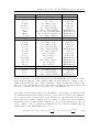
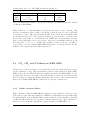
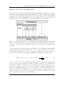
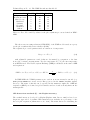
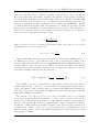
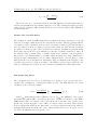

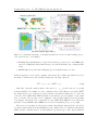
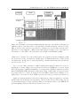
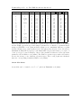
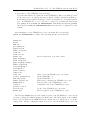
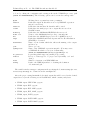


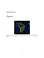
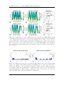
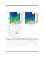
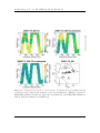

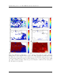

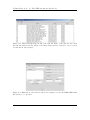
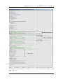


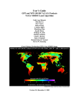


![[DRAFT] User Manual for the LMD Martian Mesoscale Model](http://vs1.manualzilla.com/store/data/005789657_1-11bdf725af45641ff39ff695d9ffff09-150x150.png)