Download Annex I Electron cooling application for luminosity preservation in an

Electron cooling application for luminosity preservation
in an experiment with internal targets at COSY.
Final report
JINR
I.N.Meshkov, A.O.Sidorin, A.V.Smirnov, G.V.Trubnikov
COSY
K.Fan, R. Maier, D. Prasuhn, H.J.Stein
Dubna, 2001
Contents
Abstract
3
Introduction
4
1. Target and beam parameters
5
2. ANKE experiment without cooling
6
7
9
2.1. Interaction with the target
2.2. Calculations in presence of intrabeam scattering
3. Beam parameter evolution with existing stochastic cooling
system
13
4. 4. Electron cooling application
16
16
20
30
4.1. Beam parameter evolution with an electron cooling
4.2. Electron cooling in experiments with the pellet target
4.3. Possible development of the existing electron cooling system
5. Electron cooling system with circulating electron beam
5.1. Magnetic field limitations
5.2. Principles of electron cooling with circulating electron beam
5.3. Storage ring with longitudinal magnetic field
5.3.1. Particle dynamics in the ring with longitudinal magnetic field.
5.3.2. Current limitation due to microwave instability
5.3.3. Transverse-longitudinal relaxation of the electron beam
5.4. Electron cooling with circulating electron beam in experiments with
internal target
5.4. Induction acceleration of the electron beam
32
32
33
35
35
38
40
41
44
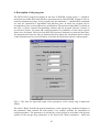
6. Principles of the electron cooling system design
45
7. Program of experiments at LEPTA
47
47
48
48
51
7.1. General parameters of the LEPTA ring
7.2. Preliminary program of experiments
7.2.1. Tuning of injection system and helical quadrupole winding
7.2.2. Study of the circulating beam dynamics
1. Role of the cooling in experiments with internal targets
2. The possibility of the existing stochastic cooling system application
3. The possibility of an electron cooling application
4. Electron cooling system with circulating beam
53
53
54
55
55
Conclusion and recommendations
56
References
58
Summary
2
Abstract
This report is dedicated to investigation of the beam parameter evolution in the experiments
with internal target. In calculations of the proton and deuteron beams we concentrated on
cluster, atomic beam, storage cell and pellet targets at ANKE experiment mainly. In these
calculations electron and stochastic cooling, intrabeam scattering, scattering on the target and
residual gas atoms are taken into account. Beam parameter evolution is investigated in the
long-term time scale, up to one hour, at different beam energies in the range from 1.0 to
2.7 GeV for proton beam and from 1 to 2.11 GeV for deuteron beam. The results of numerical
simulations of the proton and deuteron beam parameters at different energies obtained using
new version of BETACOOL program (elaborated at the first stage of this work [1]) are
presented.
Optimum parameters of the electron cooling system are estimated. The COSY experiment
requirements can be satisfied even when electron cooling time is rather long. That allows to
apply an electron cooling system with circulating electron beam [2]. Such a system has
potentially low cost in comparison with other possibilities. At the energy range from 500 keV
to 1.5 MeV only longitudinal magnetic field can provide an effective focusing of an intensive
electron beam. The electron beam acceleration can be produced both by induction
acceleration of electrons or using an RF electron LINAC. Specific limitations of such a
cooling system are discussed. Preliminary design of the electron cooling system with
circulating electron beam is described in the report.
This report contains also preliminary program of experiments at LEPTA (Low Energy
Particle Toroidal Accumulator), which are aimed to study the problems of electron cooling
system with circulating electron beam. Presently the construction of LEPTA ring is in the
final stage at JINR and experiments with circulating beam will be started the next year.
3
Introduction
The existing stochastic cooling system or an electron cooling system, which cover total
energy range of the proton or deuteron beam at COSY, can be used for the following
applications:
- at injection energy to increase the intensity of the polarized proton beam with a combined
cooling/stacking injection,
- at energy range from about 1 GeV to top energy of 2.7 GeV (2.11 GeV for deuteron beam)
for luminosity preservation in an experiment with internal targets,
- for preparation of the proton beam parameters for fast extraction in an experiment with
external target.
The ultimate possible efficiency of the beam cooling application at ANKE experiments is
investigated in the beginning of this report.
The existing COSY stochastic cooling system is successfully used now for luminosity
preservation in the COSY-11 experiment with cluster beam apparatus at relatively low proton
beam intensity. Expected target density in ANKE experiment is about one order of magnitude
higher and one plans to increase the beam intensity by upgrade the COSY injection system.
The investigation of the efficiency of the stochastic cooling system at these parameters is one
of the goals of this report. Efficiency of an electron cooling system in difference with
stochastic one does not depend on beam intensity but depends very strongly on beam energy.
Comparison between two cooling methods is the next goal of this work.
The optimum choice of the electron cooling system parameters and preliminary design of the
cooling system with circulating electron beam are also the topics of the report.
Further development of this work is experimental investigations of the electron cooling
system with circulating electron beam. We plan to investigate its problems at LEPTA (Low
Energy Particle Toroidal Accumulator) ring, which is under construction in JINR now.
LEPTA parameters are closed to estimated parameters of COSY electron cooling system. This
report contains preliminary program of experiments at LEPTA, which are aimed to study an
electron cooling system with circulating electron beam. Electron beam parameters after
injection and adjustment of the septum and kicker coils will be measured at special test bench
using optic method of the electron beam diagnostics, developed in JINR [3]. Dynamics of
circulating electron beam will be investigated when LEPTA assembling is finished.
Resonance behaviour and beam stability at injection energy will be studied using RF
acceleration of the electron beam. And final test of the cooling system will be performed after
installation of the betatron yoke. It will include the injection of electron beam, its acceleration
to maximum energy and extraction for diagnostic of the electron temperature.
Presently the construction of the general elements of LEPTA magnetic system is in the final
stage and we plan to start assembling of the ring and first experiments with electron beam in
the next year. Expected term of the experimental program completion is two years.
4
1. Target and beam parameters
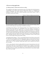
The internal targets used in COSY are listed in the Table 1.1.
Target
1. Strip or filament
2. Cluster
3. Pellet
4. Atomic beam
5. Storage cell
Table 1.1. Experiments with internal targets
COSY 11
ANKE
EDDA
filament
x
x
x
strip
x
x
x
x
The beam life time in the experiments with solid targets is so short that luminosity
preservation using the beam cooling seems to be unrealistic. All the other types of the target
will be used in the ANKE experiment and the results of the calculations for them can be
extended to other experiments with corresponding corrections the lattice functions in the
target position. Therefore in this report general attention was directed to the ANKE
experiment.
The cluster beam apparatus of ANKE experiment is very similar to COSY 11 one and
maximum designed value of target areal density was equal to 5 x 1013 atoms/ cm2. However,
the value really achieved now is substantially higher and can be estimated from of the particle
energy loss due to interaction with target using the experiment parameters (Table 1.2.). The
formula for relation between relative energy loss of the proton beam and proton revolution
frequency, one can calculate the ∆E value:
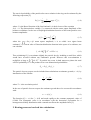
∆E 1 + γ 1 ∆f
,
=
E
γ η f
(1.1)
here η is off-momentum factor, γ is Lorenz factor.
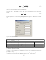
Table 1.2. ANKE experiment with hydrogen cluster beam target at January/February 2001.
Proton beam kinetic energy, GeV
2.65
Revolution frequency, MHz
1.5
-0.13
Off momentum factor, η
Frequency shift during 300 seconds, Hz
192
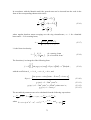
Theoretical value of the mean energy loss during single cross the target is [4]:
E

∆E = 2 ξ ln max − β 2  ,
 I

(1.2)
here Emax is the maximum energy loss in a head-on collision of the projectile with a target
electron:
5
E max =
2me c 2 β 2 γ 2
m m 
1 + 2γ e +  e 
M M 
2
,
(1.3)
me is the electron mass and M - the projectile mass, ξ is a quantity which is proportional to the
areal density ρx of the target ( – target density in g/cm3):
ξ = 0.1535
MeV cm 2 Z12 Z 2
ρx ,
g
β 2 A2
(1.4)
where, ZP and ZT are the charge number of projectile and target atoms, I is ionisation
potential: I = Z T0.9 × 16 eV
Experimental value of the energy losses follows from Formula (1.1):
∆Estr , exp =
1 + γ E ∆f T0
,
γ η f τexp
(1.5)
T0 – revolution period, τexp = 300 sec is the experiment duration.
Experimental value of the energy loss during one revolution in the ring is 7.3 meV, which
gives the target areal density of 1.3⋅1015 Atoms/cm2.
The maximum designed areal density of the storage cell is expected to be of 1014 atoms/cm2.
The frozen pellet target provides a total number of atoms per pellet of 1.8⋅1014 – 1.1⋅1016.
Influence of the target on the beam parameters can be estimated by introducing the "effective
areal density" which is proportional to ratio of the atom number per the pellet to the beam
cross section. We assume that in each moment of time one pellet is inside the beam. At the
beam emittance of 1π⋅mm⋅mrad the effective target density lies between 3⋅1014 and
2⋅1016 Atoms/cm2.
Maximum achieved intensity of the proton beam is 7⋅1010. In the future one can expect
improvement of the intensity to 1011 or even more by upgrade of the injection system. Now
the maximum beam energy is 2.65 GeV, but it is possible in the future to increase this value
to 2.7 GeV. At the same magnetic rigidity the maximum deuteron beam energy is 2.11 GeV.
Thus, in this report the calculations of the beam parameters were fulfilled at target density
from 1015 to 1016 Atoms/cm2 (at lower value the experiment can be performed during long
time duration without cooling), at the beam intensity up to 1011 particles and in the beam
energy range from 1 GeV to 2.7 GeV for protons and to 2.11 GeV for deuterons. The ring
acceptance was taken of 10-5 π⋅m⋅rad in the both planes, which is corresponds to expected
aperture of the gas storage sell. The initial beam parameters were taken approximately
corresponded to these ones after acceleration: emittances of 10-6 π⋅m⋅rad in the both planes
and momentum spread of 10-4.
6
2. ANKE experiment without cooling
Efficiency of the cooling application at experiment with internal target is determined by
relation between different sources of the particle losses. Generals of them are the following:
- single scattering on the target atoms on a large angle,
- the same for residual gas atoms,
- emittance growth and aperture limitation,
- momentum spread growth and limitation of longitudinal acceptance.
The particle losses due to single scattering on the target atoms restricts the experiment
duration and can not be effected by the beam cooling. Emittance and momentum growth can
be compensated by stochastic or electron cooling. In this case luminosity life time is
determined only by single scattering process. The sources of the beam phase volume growth
are the multiple scattering on residual gas and the target atoms, intrabeam scattering.
First of all influence of residual gas on the beam life time was investigated under assumption
that average pressure in COSY vacuum chamber is 5⋅10-9 Torr and gas composition is 95% of
hydrogen and 5% of nitrogen. At these conditions the particle life time is about 106 seconds
and emittance growth rate at minimum beam energy of 1 GeV is about 3⋅10-10 π⋅m⋅rad/sec.
Thus the interaction with the residual gas does not restrict particle life time and slightly
influences on the particle losses due to emittance growth.
2.1. Interaction with the target
Ultimate efficiency of the beam cooling can be estimated in the case of high target density
and low intensity of the ion beam – in this case beam parameters are determined only by
interaction with the target. Multiple scattering on the target atoms leads to the linear in time
growth of the beam emittance and particle losses takes place when the beam emittance
increases up to 0.3 of the ring acceptance [4]. The period of time when the emittance growth
does not lead to the particle losses can be estimated by the following formula:
τ=
Aτ ε
,
3ε
(2.1)
which gives the time of emittance growth from zero value to acceptance limit. Here A is the
ring acceptance, τε is the characteristic time of the emittance growth calculated at certain
value of the beam emittance ε.
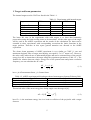
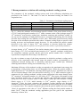
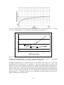
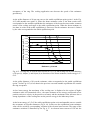
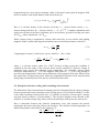
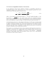
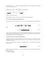
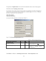
Fig. 2.1, 2.2 show the characteristic times of the single scattering process and emittance
growth up to acceptance limit in both planes for proton and deuteron beam. The ring
acceptance was taken of 10-5 π⋅m⋅rad in the both planes. The beta functions of the ring at the
target position were taken of 2 meters in the horizontal plane and of 3 meters in the vertical
one. The presented values correspond to the hydrogen target at the areal density of
1016 Atoms/cm2 and beam emittances of 10-6 π⋅m⋅rad in the both planes. All the characteristic
times are linearly scaled with the target density and can be simply recalculated to each
required value. The difference in the energy dependence of the single and multiple scattering
life times appears because of in the single scattering life time calculation the particle losses
due to nuclear scattering are taken into account. The difference between horizontal and
7
Characteristic times, sec
vertical degrees of freedom is explained by the difference in the beta functions in the target
position.
500
1
400
300
2
200
3
100
0
0
1
2
3
Beam energy, GeV
Characteristic times, sec
Fig. 2.1. The proton beam life time due to single scattering on the target atoms (1) and the
times of emittance growth up to the acceptance limit in horizontal (2) and in vertical (3)
planes.
350
300
250
200
150
100
50
0
1
2
3
0
0.5
1
1.5
2
2.5
Beam energy, GeV
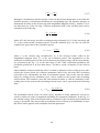
Fig. 2.2. The deuteron beam life time due to single scattering on the target atoms (1) and the
times of emittance growth up to the acceptance limit in horizontal (2) and in vertical (3)
planes.
For both kinds of particles (protons and deuterons) the experiment duration is limited by
about 5 minutes at the target density of the order of a few 1016 Atoms/cm2 and by about 1
hour at the target density of about 1015 Atoms/cm2. Correspondingly in the following
8
calculations we will investigate two cases: short term beam parameter evolution at high target
density and long term evolution at low target density.
For both beams in the total energy range the particle losses due to aperture limitation play a
significant role and suppression of the emittance growth by the beam cooling can increase the
integral luminosity of the experiment by several times. Ultimate possible efficiency of the
cooling decreases with the increase of the beam energy, and for deuteron beam at maximum
energy the maximum gain in the luminosity is less than two times.
More accurate estimations of the possible cooling efficiency at high beam intensity have to
include consideration of the intrabeam scattering process.
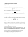
2.2. Calculations in presence of intrabeam scattering
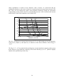
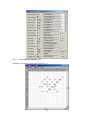
The intrabeam scattering calculations are performed for the lattice parameters given in
Fig. 2.3. Initial beam parameters in the numerical investigations were chosen the following:
beam emittance in the both planes is equal to 10-6 π⋅m⋅rad, momentum spread is equal to 10-4.
Calculations were performed taking into account the beam interaction with residual gas and
target atoms and intrabeam scattering in the ion beam. The initial beam intensity was chosen
to be equal maximum expected value of 1011 particles. An example of the calculations of
short term variation of the beam parameters at the target areal density of 1016 Atoms/cm2 is
presented in the Fig. 2.4 for proton beam at energy of 2.7 GeV.
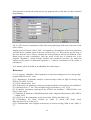
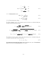
βhor, m
Ecool ANKE
βvert, m
D, m
Fig 2.3. Lattice parameters at ANKE experiment, Q = 3.571, γtr = 2.243.
In the cooling section: Beta-functions = 13/15 m, Dispersion = 0,
in ANKE: Beta-functions = 2/3 m, Dispersion = 0
9
εhor
εvert
Fig. 2.4. The dependencies of the proton beam emittance (a), momentum spread (b) particle
number (c) on time, target density is 1016 Atoms/cm2.
One can see that after five minutes of experiment the beam emittance is limited by the ring
acceptance, and the particle number decreases from 1011 to 3.6⋅1010. The particle number after
five minutes of experiment calculated without taking into account aperture limitation is equal
10
to 4.85⋅1010. The ratio between final particle number calculated without and with the aperture
limitation can be used as a parameter, which characterises the gain in the experiment
luminosity when the cooling completely suppresses the emittance growth. The ultimate
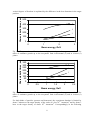
possible cooling effect on the experiment (ratio of the beam intensity with cooling to that one
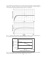
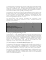
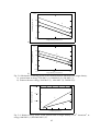
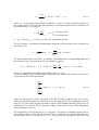
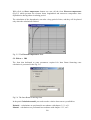
without cooling) at high target density is presented in the Fig. 2.5. The possible gain in the
particle number after one hour of experiment at the target density of 1015 Atoms/cm2 is
presented in the Fig 2.6.
One can see that the beam cooling can provide maximum gain in the beam intensity at
minimum beam energy and for the proton beam, where this value is up to ten times. The gain
for deuteron beam is about two times less due to intrabeam scattering dependence on the
particle mass. At maximum energy the gain decreases to the value of about 50%. It is
explained by the strong dependence of the intrabeam scattering on energy (as β3γ4). As result
at maximum beam energy the emittance growth due to this process does not play a significant
role. The difference between hydrogen and deuterium targets is negligible because of the
main processes are determined by the interaction of the beam with electrons of the target
atoms.
In the presented version of the numerical program the particle losses due to longitudinal
acceptance limitation are not taken into account, correspondingly presented calculations can
underestimate the particle losses due to growth of the momentum spread.
Gain in the intencity
The next chapters of the report are dedicated to calculations of the beam parameter evolution
in the presence of stochastic or electron cooling.
9
8
7
6
5
4
3
2
1
0
1
2
0
1
2
3
Beam energy, GeV
Fig. 2.5. Ultimate gain in the beam intensity which can be obtained using cooling at the
experiment duration of 5 minutes: 1 – proton beam, 2 – deuteron beam. The hydrogen target
density is 1016 Atoms/cm2, initial beam intensity is 1011 particles.
11
Gain in the intensity
14
13
12
11
10
9
8
7
6
5
4
3
2
1
0
1
2
0
1
2
3
Beam energy, GeV
Fig. 2.6. Ultimate gain in the beam intensity which can be obtained using cooling at the
experiment duration of 1 hour: 1 – proton beam, 2 – deuteron beam. The hydrogen target
density is 1015 Atoms/cm2, initial beam intensity is 1011 particles.
12
3. Beam parameter evolution with existing stochastic cooling system
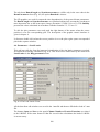
The parameters of the stochastic cooling system used in the following calculations are
presented in the Table 3.1. The band I is used for horizontal cooling, the Band II for
longitudinal one.
Lower frequency, GHz
Upper frequency, GHz
Bandwidth, GHz
Table 3.1. Parameters of stochastic cooling system
Band I
Band II
1
1
1.8
3
0.8
2
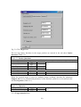
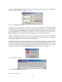
Fig. 3.1. shows the emittance and momentum spread evolution of the proton beam at energy
of 1 GeV and initial particle number of 1011 under common action of the hydrogen target of
1016 Atoms/cm2 areal density, residual gas, intrabeam scattering and stochastic cooling. As
one can see the emittances in both plane increase to acceptance limit during first 30 seconds
and after that cooling does not influence on this value. Momentum spread increases during
first part of the calculation period but after about 3 minutes cooling begins to prevail on the
heating processes and momentum spread decreases. To this moment the particle number
decreases to the value of about 2⋅1010 and continues to decrease during last minutes.
Stochastic cooling does not influence on the particle losses at these experiment parameters.
At target density of 1016 Atoms/cm2 the similar situation takes a place at maximum proton
beam energy of 2.7 GeV and initial beam intensity of 1011 particles: stochastic cooling does
not compensate emittance growth, and the gain in the particle number after 5 minutes of
experiment accompanied with cooling is less than 10%.
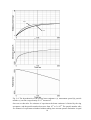
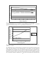
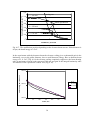
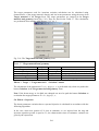
In order to estimate a range of the beam parameters in which the stochastic cooling can be
effective in the experiment with internal target the particle number corresponding to an
equilibrium between heating due to interaction with the target, residual gas, intrabeam
scattering and stochastic cooling was calculated (Fig. 3.2, 3.3).
Maximum efficiency of the stochastic cooling corresponds to the maximum beam energy due
to dependence of the mixing factor on off momentum factor. When the particle number is
higher than about 1010 the intrabeam scattering (IBS) begins to play a significant role, that one
can see from the change of the curve derivatives in the Fig. 3.2, 3.3. More attractive region of
parameters for the existing stochastic cooling system application is the target density below
1015 Atoms/cm2 and particle number of a few units of 1010. This region corresponds to long
term experiment and the Fig. 3.4 presents the emittance and momentum spread evolution
during one hour under common action of IBS, target, residual gas and stochastic cooling.
(Beam energy is 2.7 GeV, initial intensity is 2⋅1010 particles, target density is 1015
Atoms/cm2.) After the beam relaxation the stochastic cooling stabilises the horizontal
emittance and the momentum spread, vertical emittance increases during the first 30 minutes
to acceptance limit. The computer simulation shows that the particle number decreases during
1 hour of experiment to the value of 7.4⋅109. Without cooling the final particle number is
about 5.6⋅109. Thus the stochastic cooling application gives the gain in the experiment
luminosity of about 30%.
13
As a conclusion from this analysis one can expect effective application of existing stochastic
cooling in the experiment with internal target when the beam intensity is about or below of
2⋅1010 particles, and the target density does not exceed 1015 Atoms/cm2.
εhor
εvert
Fig. 3.1. Emittance and momentum spread evolution at stochastic cooling. Target density is
1016 Atoms/cm2, beam energy 1 GeV, the beam intensity is 1011 protons.
Proton number
1.0E+11
1.0E+10
1.0E+09
1.0E+08
1.0E+14
1.0E+15
1.0E+16
Target density, Atoms/cm^2
Fig. 3.2. Proton number corresponding to equilibrium between heating effects and stochastic
cooling in the horizontal degree of freedom. Beam energy is 2.0 GeV.
14
Proton number
1.0E+11
1.0E+10
1.0E+09
1.0E+14
1.0E+15
1.0E+16
Target density, Atoms/cm^2
Fig. 3.3. Proton number corresponding to equilibrium between heating effects and stochastic
cooling in the horizontal degree of freedom. Beam energy is 2.7 GeV.
2
1
Fig. 3.4. Emittance (1 - horizontal, 2 - vertical) and momentum spread evolution. Target
density is 1015 Atoms/cm2, beam energy 2.7 GeV, initial beam intensity is 2⋅1010 protons.
15
4. Electron cooling application
4.1. Beam parameter evolution with an electron cooling
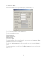
The calculations in this chapter were performed at the electron beam and solenoid parameters
corresponding to the existing COSY electron cooling system (Table 4.1). Longitudinal and
transverse temperature were chosen using the results of the friction force measurements
performed at COSY in May 2001. Only the maximum electron beam energy is varied in
accordance with the proton energy.
Effective length of the cooling section, m
Maximum magnetic field value, kG
Maximum value of electron beam current, A
Electron beam radius, cm
Transverse electron temperature, meV
Longitudinal electron temperature, meV
Neutralisation factor, %
Beta functions in the cooling section, m
Table 4.1. Electron cooling system parameters.
1.4
1.2
3
1.26
300
10
30
13/15
The beam parameter evolution is calculated taking into account all general heating effects:
interaction with residual gas, internal target and intrabeam scattering.
At minimum proton energy of 1 GeV and target density of 1016 Atoms/cm2 the value of the
electron beam current required for compensation of the beam heating in all degrees of
freedom is of the order of a few Amperes. Fig. 4.1 presents the emittance and momentum
spread evolution during 5 minutes of experiment at electron beam current of 1.5 A. After the
relaxation of the beam parameters at initial stage the emittances and momentum spread keep
to be the constant values during long time and the particle losses are determined only by the
single scattering on the target atoms. In this range of parameters electron cooling application
have a maximum efficiency and after five minutes of experiment it allows to have proton
beam of 10 times higher intensity than without cooling.
At maximum proton energy (2.7 GeV) even maximum electron beam current can not provide
the stabilisation of the emittance and momentum growth. However at electron beam current of
3 A (Fig. 4.2) the heating processes are substantially suppressed and gain in the particle
number after five minutes of experiment is about 20% which is close to maximum achievable
value (see Fig. 2.5). The experiment at high target density will be considered more detail in
the next chapter.
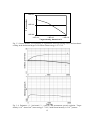
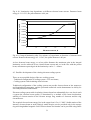
At lower target density the electron cooling stabilises the proton beam parameters in the total
energy range. In the Fig. 4.3 the equilibrium beam parameters as a function of beam energy
are presented. The electron beam current was chosen to obtain equilibrium proton beam
emittance of about 10-6 π⋅m⋅rad. The equilibrium is reached during about 10 minutes and after
that emittance and momentum spread slowly decrease with decrease of the particle number
due to losses in the target.
16
εvert
εhor
Fig. 4.1. Proton beam parameter time dependencies. Proton number is 1011, energy is 1 GeV,
target density is 1016 Atoms/cm2. Electron beam current is 1.5 A.
εvert
εhor
Fig. 4.2, a. Proton beam emittance time dependencies. Proton number is 1011, energy is
2.7 GeV, target density is 1016 Atoms/cm2. Electron beam current is 3 A.
17
Fig. 4.2, b. Proton beam momentum spread time dependencies. Proton number is 1011, energy
is 2.7 GeV, target density is 1016 Atoms/cm2. Electron beam current is 3 A.
3.5
3
3
2.5
2
1
1.5
1
2
0.5
0
0.5
1
1.5
2
2.5
3
Beam energy, GeV
Fig 4.3. Equilibrium proton beam parameters as a function of the beam energy.
1 –horizontal emittance in 10-6 π⋅m⋅rad, 2 – vertical emittance in 10-6 π⋅m⋅rad, 3 – momentum
spread in 10-4. Proton number is 1011, target density 1015 Atoms/cm2.
Analogous dependencies for deuteron beam are presented in the Fig. 4.4. In the first
approximation the cooling time for deuterons is two times longer than for protons, but
charcteristic time of the emittance growth due to multiple scattering with the target atoms is
longer by four times. As result the electron beam current required to obtain the equilibrium is
about two times lower. The values of the electron beam current used in the calculations of the
Fig 4.3 – 4.4 are presented in the Fig. 4.5. The equilibrium is reached in the case of deuteron
beam during 20 – 30 minutes and this time is comparable with the particle life time due to
single scattering on the target atoms.
18
1.8
1.6
3
1.4
2
1.2
1
0.8
1
0.6
0.4
0.2
0
1
1.2
1.4
1.6
1.8
2
2.2
Beam ene rgy, GeV
Fig 4.4. Equilibrium deuteron beam parameters as a function of the beam energy.
1 – horizontal emittance in 10-6 π⋅m⋅rad, 2 – vertical emittance in 10-6 π⋅m⋅rad, 3 – momentum
spread in 10-4. Deuteron number is 1011, target density 1015 Atoms/cm2.
Electron beam current, mA
700
600
500
400
Deuterons
Protons
300
200
100
0
1
1.5
2
2.5
3
Beam energy, GeV
Fig. 4.5. The electron beam current required to reach the equilibrium emittance in both planes
of about 10-6 π⋅m⋅rad.
The stabilization of the ion beam parameters is important in the experiment with cluster beam
target. The target dimension in the horizontal plane is less than the ion beam dimension
corresponding to the acceptance limit. The numerical model used in these calculations does
not permit to solve the problem correctly in the case, when the horizontal emittance is varied
during the experiment. However one can estimate possible gain in the experiment luminosity
due to horizontal emittance stabilization as a ratio between maximum beam dimension and
19
target dimension. This ratio is about 1.5 – 2 and taking into account that the characteristic
time of emittance growth without cooling is about 10 minutes the gain in the luminosity can
be estimated by the value 1.5.
The electron beam radius of 1.26 cm required for electron cooling at injection energy is more
than two times bigger than ion beam one at experiment with internal target. Decrease of the
electron beam radius permits to decrease the beam current. In the experiments with gas jet and
cluster targets this fact does not play a significant role due to small value of the electron beam
current density required for effective cooling. In the experiment with higher target density and
at maximum beam energy the electron beam current density has to be as high as possible and
an accurate choice of the electron beam radius is necessary to minimize the electron beam
current. The optimum electron beam parameters will be discussed below.
4.2. Electron cooling in experiments with the pellet target
In the experiment with the pellet target the effective target density depends on the beam cross
section and as a result its value is changed when the beam emittance is varied.
Correspondingly the efficiency of electron cooling system can be substantially higher in the
case, when the cooling suppresses the heating effects. In the previous chapter the electron
cooling efficiency in the experiment with high target density was considered only from the
side of the suppression the particle losses due to acceptance limitation and effective target
density was assumed to be constant. In this chapter we investigate the experiment with the
pellet target taking into account variation of the effective target density.
In this chapter the parameters of the electron cooling system presented in the Table 5
(chapter 5) are used in the simulations. The proton beam intensity is 1011 particles, which
corresponds to the expected value after installation of new injection system.
The luminosity of the experiment with pellet target is determined by the expression:
L=
Nb Nt
P,
S t Trev
(4.1)
where Nb is the particle number in the beam, Trev – revolution period, Nt is particle number in
the target, St – target cross-section, P – probability of the particle cross the target.
Assuming that the pellets cross the beam one by one with the period equal to the time duration
of the beam crossing by a pellet, one can estimate the probability as the following:
P=
St
St
≈
S b π β xε x β y ε y
(4.2)
where βx,y –horizontal and vertical beta functions in the target position (dispersion in the
target position is closed to zero), εx,y – corresponding two-sigma emittances. As a result we
have:
L=
Nb Nt
πTrev β x ε x β y ε y
20
(4.3)
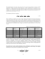
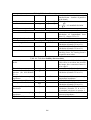
The pellet diameter lies in the range from 20 to 80 µm, the target density is about 1.4⋅1022
Atoms/cm3. Target parameters and luminosity of the experiment are presented in the
Table 4.2. The luminosity is calculated under assumption that one pellet is in the beam, beam
emittance is 1 π⋅mm⋅mrad in the both transverse planes, the proton beam intensity is 1011
particles and beam energy is 2.7 GeV.
The luminosity life time is equal to:
1 dL
1 dN b 1 dε x
1 dε y
=
−
−
.
L dt N b dt
ε x dt ε y dt
(4.4)
Thus, in difference with the case of gas storage cell target the luminosity life time depends not
only on the particle life time, but also on the emittance variation. At optimum experiment
conditions the electron cooling can provide practically constant luminosity during long period
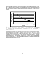
of time by corresponding choice of the electron beam current. In the Fig. 4.6 the luminosity of
the experiment at maximum beam energy is presented for pellet diameter of 40 µm and
50 µm.
Table 4.2. The pellet target parameters
Pellet diameter, Number
particles
µm
20
1.8⋅1014
30
5.94⋅1014
40
1.43⋅1015
50
2.75⋅1015
60
4.84⋅1015
70
7.54⋅1015
80
1.1⋅1016
of Target
cross- Target
section, cm2
cm
-6
0.00157
3.14⋅10
0.00236
7.07⋅10-6
-5
0.00314
1.26⋅10
-5
0.00393
1.96⋅10
-5
0.00471
2.83⋅10
-5
0.0055
3.85⋅10
-5
0.00628
5.03⋅10
length, Luminosyty,
cm-2*sec-1
3.66⋅1032
1.21⋅1033
2.91⋅1033
5.6⋅1033
9.85⋅1033
1.54⋅1034
2.32⋅1034
At pellet diameter of 40 µm electron cooling compensate the particle losses by corresponding
decrease of the beam emittance and the experiment luminosity variation during first five
minutes is negligible. At the same conditions without electron cooling the luminosity
decreases by about 3 times. At bigger pellet diameter the power of electron cooling is not high
enough to suppress the beam heating due to interaction with target and the cooling application
leads only to some increase of the luminosity life time.
The effectiveness of the cooling application can be estimated by comparison of an integral
luminosity after certain period of experiment with and without of the cooling. The integral
luminosity for some period of experiment can be calculated:
Lint =
Texp
Nt
πTrev β x β y
21
∫
0
Nb
ε xε y
dt .
(4.5)
Or in the case of numerical integration of the beam dynamics
Lint =
∆t
π β x β y Trev
Nt
n
∑
i =1
Nb
ε xε y
,
(4.6)
where ∆t is integration step over time, n is the number of the integration steps.
Luminosity, 1/cm^2*sec
3.50E+33
3.00E+33
2.50E+33
2.00E+33
Ie = 0
Ie = 0.5 A
1.50E+33
1.00E+33
5.00E+32
0.00E+00
0
50
100
150
200
250
300
Time, sec
6.00E+33
Luminosity, 1/cm^2*sec
5.00E+33
4.00E+33
Ie = 0
3.00E+33
Ie = 0.5 A
2.00E+33
1.00E+33
0.00E+00
0
50
100
150
200
250
300
Time, sec
Fig. 4.6. Luminosity time dependence at pellet diameter of 40 µm (upper plot) and 50 µm
(bottom plot), proton beam energy is 2.7 GeV.
The gain in the integral luminosity after five minutes of the experiment provided by the
cooling application (Fig. 4.7, 4.8) is several times at pellet diameter less than 50 µm, and
decreases to about 10% at bigger pellet diameter. At the pellet diameter less than 40 µm the
electron beam current of 500 mA is not optimal to obtain maximum luminosity that explains
peculiarity of the curve in the Fig. 4.7. The dependence of the luminosity on the electron
beam current will be discussed more detail below.
22
At big target density, when the cooling only slightly influences on the beam parameters
during experiment, the cooling system can be used also for preliminary preparation the beam
parameters before the target switching on. All the previous estimations were performed at the
following initial beam parameters: emittances in both planes are 1 π⋅mm⋅mrad and
momentum spread is 10-4. The beam parameters corresponding to the equilibrium between
electron cooling and intrabeam scattering are the foolowing: horizontal emittance is about 0.3
π⋅mm⋅mrad, vertical emittance - 0.1 π⋅mm⋅mrad and momentum spread is about 8⋅10-5. The
equilibrium is reached during 30 – 60 sec depending on initial beam parameters. Without the
target the beam life is higher than 105 sec and permits to perform all required manipulations
of the beam parameters.
Integral luminosity, 1/cm^2
1.80E+36
1.60E+36
1.40E+36
1.20E+36
1.00E+36
Ie = 0
8.00E+35
Ie = 0.5 A
6.00E+35
4.00E+35
2.00E+35
0.00E+00
0
20
40
60
80
100
Pellet diameter, um
Fig. 4.7. Integral luminosity after five minutes of experiment as a function of the pellet
diameter, beam energy is 2.7 GeV.
Gain in integral luminosity
4.5
4
3.5
3
2.5
2
1.5
1
0.5
0
0
20
40
60
80
100
Pellet diameter, um
Fig. 4.8. Gain in the integral luminosity after five minutes of the experiment at electron beam
current of 0.5 A, proton beam energy is 2.7 GeV.
23
In the Fig. 4.9 the integral luminosity was calculated under assumption that emittances in the
both planes are the same and momentum spread is 10-4. The integral luminosity
monotonically increases with the decrease of the initial beam emittance and expected gain
after five minutes of experiment due to initial preparation the beam before experiment is
about 10%.
Integral luminosity
1.70E+36
1.65E+36
1.60E+36
1.55E+36
1.50E+36
1.45E+36
0
0.2
0.4
0.6
0.8
1
1.2
1.4
1.6
Initial emittance, pi*mm*mrad
Fig. 4.9. Integral luminosity in 1/cm2 after five minutes of experiment without cooling as
function of initial beam emittance, beam energy is 2.7 GeV, pellet diameter is 80 µm.
In order to obtain maximum integral luminosity one can to optimise the experiment duration
also. The integral luminosity increases approximately as a square root from the experiment
duration (Fig. 4.10). Maximum gain in the luminosity obtained due to beam cooling before
experiment corresponds to short term of the experiment, and it decreases with increase of the
experiment duration (Fig. 4.11).
1.80E+36
Integral luminosity, 1/cm^2
1.60E+36
1.40E+36
1.20E+36
0.3
1
1.5
1.00E+36
8.00E+35
6.00E+35
4.00E+35
2.00E+35
0.00E+00
0
50
100
150
200
250
300
Time, sec
Fig. 4.10. Integral Luminosity as function of the experiment duration depending on initial
beam emittance in π⋅mm⋅mrad, beam energy is 2.7 GeV, pellet diameter is 80 µm, cooling is
off.
24
Thus, even at big target density, when the cooling power is not enough to suppress the heating
due to interaction with the target, the experiment luminosity can be improved by preparation
the beam parameters before the target switching on and by optimization of the experiment
scenario.
4
Gain in integral luminosity
3.5
3
2.5
2
1.5
1
0.5
0
1
10
100
1000
Time, sec
Fig. 4.11. The ratio between the integral luminosity at initial emittance of 0.3 π⋅mm⋅mrad and
1.5 π⋅mm⋅mrad versus experiment duration, beam energy is 2.7 GeV, pellet diameter is
80 µm, cooling is off.
At maximum experiment energy the luminosity increases with the electron beam current and
maximum luminosity corresponds to maximum electron beam current. The electron cooling
efficiency increases with decrease of the experiment energy (Fig. 4.12). And at minimum
experiment energy it is not necessary to have maximum electron beam current to obtain the
maximum luminosity – the luminosity dependence on the current has a saturation in the
region of 400 mA (Fig. 4.13). The reason of the saturation can be explained by analysis of the
luminosity time dependence (Fig. 4.14).
25
Gain in integral luminosity
1.8
1.7
1.6
1.5
1.4
1.3
1.2
1.1
1
1
1.5
2
2.5
Beam energy, GeV
Fig. 4.12. Gain in integral luminosity after five minutes of experiment at electron beam
current of 0.5 A, pellet diameter is 80 µm.
Gain in integral luminosity
1.8
1.7
1.6
1.5
1.4
1.3
1.2
1.1
1
0
0.1
0.2
0.3
0.4
0.5
Electron beam current, A
Fig. 4.13. The gain in integral luminosity after five minutes of experiment as function of
electron beam current, beam energy is 1 GeV, pellet diameter is 80 µm.
26
Luminosity, 1/cm^2*sec^-1
2.5E+34
2.0E+34
Ie=0
1.5E+34
Ie=0.5A
Ie=0.4A
1.0E+34
Ie=0.3A
5.0E+33
0.0E+00
0
50
100
150
200
250
300
Time, sec
Fig. 4.14. Luminosity time dependencies at different electron beam current, beam energy is
1 GeV, pellet diameter is 80 µm.
At the electron beam current of 0.3 A the beam heating due to interaction with the target
prevails on the cooling and beam emittance increases during experiment, but not so fast as
without cooling. This “deceleration” of the emittance growth gives some gain in the
luminosity life time in accordance with formula 4.4. At the electron beam current of 0.4 and
0.5 A the electron cooling completely suppresses the emittance growth and at the first stage of
experiment (about 20 sec) the beam emittance decreases to the equilibrium value. The
equilibrium is determined by the electron beam current and at 0.5 A it corresponds to about
0.62 π⋅mm⋅mrad in the horizontal plane and 0.88 π⋅mm⋅mrad in the vertical one. At the
electron beam current of 0.4 A equilibrium emittances have some higher values: 0.7
π⋅mm⋅mrad - horizontal and 0.98 π⋅mm⋅mrad - vertical. After reaching the equilibrium
luminosity decreases with the life time determined only by single scattering losses in the
target. These losses is proportional to the probability of the particle cross the target, and,
therefore, inversely proportional to the beam emittance. Thus, the initial gain in the
luminosity, when the beam emittance decreases, is compensated by the shorter luminosity life
time after reaching the equilibrium. It means that at the elevated beam energy and (or)
relatively small target density the electron beam current has to be optimised to obtain
maximum integral luminosity at each given experiment duration.
The possibility to vary the beam emittance during experiment can be investigated by
comparison between the electron cooling rate and heating rate due to interaction with the
target. In the Fig. 4.15 the dependencies of cooling and heating rate on the beam emittance at
the beam energy of 2.7 GeV are presented.
At the pellet diameter of 80 µm (curve 4 in the Fig. 4.15) the heating always prevails on the
cooling (curve 1), equilibrium is impossible and emittance of the beam increases to
27
acceptance of the ring. The cooling application can decrease the speed of the emittance
growth only.
At the pellet diameter of 40 µm one can see the stable equilibrium point (point 1 in the Fig.
4.15) and unstable one (point 2). When the beam emittance value is less than certain value
corresponded to the unstable equilibrium the emittance of the beam decreases under common
action of the cooling and target to the stable equilibrium point. When the beam emittance is
less than its value in the stable equilibrium, it increases, but the emittance increase is limited
by the value corresponded to the stable equilibrium point.
Cooling (heating) rate, sec^-1
0.05
4
3
2
0.045
0.04
0.035
1
0.03
3
0.025
1
0.02
0.015
0.01
0.005
0
1.0E-08
2
1.0E-07
1.0E-06
1.0E-05
Emittance, pi*m*rad
Fig. 4.15. Cooling rate at electron beam current of 0.5 A (1) and heating rate at pellet diameter
of 20 µm (2), 40µm (3) and 80µm (4) as functions of the beam emittance, beam energy is 2.7
GeV.
At the pellet diameter of 20 µm the emittance value corresponded to the stable equilibrium
(point 3 in the Fig 4.15) is less than in the previous case and unstable equilibrium lies outside
the ring acceptance.
At low beam energy the maximum of the cooling rate is displaced to the region of higher
emittances (this is a kinematical effect – the same emittance at low energy corresponds to low
particle transverse velocity in the particle rest frame) and the maximum value increases due to
strong dependence of the cooling time on the particle energy in the laboratory frame.
At the beam energy of 1 GeV the stable equilibrium points exist and unstable ones are outside
the acceptance at all pellet diameters (Fig. 4.16). In this case the equilibrium beam emittance
value can be varied by corresponding variation of the electron beam current. The range of the
emittance variation is illustrated by the Fig. 4.17. At electron beam current of 150 mA the
28
stable equilibrium is reached at the emittance value of about 1.5 π⋅mm⋅mrad and the
equilibrium displaces to the value of about 0.8 π⋅mm⋅mrad at the electron beam current of 500
mA. Thus, one can obtains the regime with permanent luminosity during the experiment
compensating of the particle losses by corresponding increase of the electron beam current
(and decrease of the beam emittance) (see formula 4.4).
0.2
2
3
4
0.18
0.16
stable equilibrium
0.14
0.12
0.1
0.08
1
0.06
0.04
0.02
0
1.00E-08
1.00E-07
1.00E-06
1.00E-05
Emittance, pi*m*rad
Fig. 4.16. Cooling rate at electron beam current of 0.5 A (1) and heating rate at pellet diameter
of 20 µm (2), 40µm (3) and 80µm (4) as functions of the beam emittance, beam energy is
1 GeV.
The Fig. 4.15 – 4.17 are plotted without taking into account intrabeam scattering in the proton
beam. However, the intrabeam scattering at the beam intensity up to 1011 particles slightly
displaces the equilibrium position only.
29
Cooling (Heating) rate, sec^-1
0.14
heating rate
Ie = 500 mA
0.12
0.1
stable equilibrium
0.08
Ie = 250 mA
0.06
0.04
Ie = 150 mA
0.02
0
1.00E-07
1.00E-06
1.00E-05
Emittance, pi*m*rad
Fig. 4.17. The equilibrium position depending on the electron beam current. Pellet diameter is
80 µm, the beam energy is 1 GeV.
In the experiments with the deuteron beam the electron cooling gives a substantial gain in the
luminosity even at big pellet diameter, due to small deuteron energy. But at deuteron beam
energy of 2.11 GeV (Fig. 4.18) the electron cooling completely suppresses the beam heating
only at maximum electron beam current of 500 mA and gain in the integral luminosity after
five minutes of the experiment is about 50% (Fig. 4.18).
Luminosity, cm^-2*sec^-1
1.0E+35
Ie = 0
Ie = 0.3A
1.0E+34
Ie = 0.4A
1.0E+33
0
50
100
150
Time, sec
30
200
250
300
Fig. 4.18. Luminosity time dependence at different electron beam current. Deuteron beam
energy is 2.11 GeV, the pellet diameter is 80 µm.
Integral luminosity, cm^-2
1.9E+36
1.8E+36
1.7E+36
1.6E+36
1.5E+36
1.4E+36
1.3E+36
1.2E+36
1.1E+36
1.0E+36
0
0.1
0.2
0.3
0.4
0.5
Ele ctron current, A
Fig. 4.19. Integral luminosity after five minutes of experiment as function of electron beam
current. Deuteron beam energy is 2.11 GeV, the pellet diameter is 80 µm.
At less deuteron beam energy or at less pellet diameter the maximum gain in the integral
luminosity can be achieved at less electron beam current and, as in the case with the proton
beam, maximum expected gain in the luminosity can be 3 – 4 times.
4.3. Possible development of the existing electron cooling system
There are two possible design of the new cooling system:
- Traditional configuration of cooling system + HV accelerator,
- Cooling system with circulating electron beam.
Traditional configuration of the cooling system can provide electron beam at low transverse
and longitudinal temperature, and the presented numerical results demonstrate its ability for
ion beam parameters stabilization.
Electron cooling system with circulating electron beam has substantially low cost, but in such
a system the electron beam quality is determined by a method of the beam acceleration,
stability of electron motion in the electron storage ring, number of electrons and the ring
circumference.
The required electron beam energy lies in the range from 0.5 to 1.5 MeV. Stable motion of the
intensive electron beam at such relatively small energies can be provided only in the storage
ring with longitudinal magnetic field. Electron beam acceleration can be provided using linear
31
RF accelerator which periodically fills up the ring with new portion of electrons, or directly in
the electron storage ring using induction acceleration.
In the first case longitudinal temperature of the electron beam can be even higher than
transverse one, and one of the general problems of this method is to adjust the momentum
spread of the electron beam with the ring dynamic aperture on momentum deviation.
Induction acceleration of the electron beam permits to keep the flattened velocity distribution
of the electrons and in principle provides the same longitudinal temperature as HV
accelerator. However at constant value of the guiding magnetic field the working point
crosses resonance regions of the Larmor oscillations. Due to this fact the transverse
temperature of the electron beam can be higher than one in traditional cooling system by
several orders of magnitude.
The design of the electron cooling system of traditional configuration was performed at
COSY earlier [5]. The following chapters of this report are dedicated to investigation of
cooling efficiency at relatively pure electron beam quality. The brief description of the
cooling method with circulating electron beam and preliminary design of the installation are
given.
32
5. Electron cooling system with circulating electron beam
The choice of the electron cooling system parameters is restricted by number of
limitations. Part of them is common for both systems: with single pass and with
circulating electron beam.
First of all it is requirement of the beam magnetisation, which limits the minimum value
of the longitudinal magnetic field and maximum value of electron beam current.
Other limitations are related only to the system with circulating electron beam and
particle dynamics in the storage ring with longitudinal magnetic field. Generals of them
are the following:
- upper limit of the electron beam circulation period determined by increase of electron
temperature during cooling process,
- upper limit of the electron beam momentum spread determined by dynamic aperture
of the ring,
- upper limit of the electron beam current determined by threshold of microwave
instability,
- limitations of the magnetic field and electron beam current due to longitudinaltransverse relaxation of the electron beam.
5.1. Magnetic field limitations
Electron beam magnetization is an efficient way of electron cooling rate increase using of
longitudinal magnetic field [6] for transportation of the electron beam from the gun cathode to
the collector through drift chambers including cooling section. The criterion of electron beam
33
magnetization has a clear physics meaning: radius of electron Larmor spiral in magnetic field
has to be smaller of the mean distance between electrons [6]:
13
ρ ≤ (ne )
−1 3
when B > Bmin 1 ≡
 Ie 
m

T⊥mc2 
2 
e
 βγπa ec 
.
(5.1)
Here ne is electron density in the electron rest frame, Ie – electron beam current, e, m –
(
)
−1 2
2
electron charge and mass, βc – electron velocity, γ = 1 − β
. Computer simulations with
single pass electron beam show significant, up to several times, growth of cooling rate when
B ⇒ Bmin1 and its saturation at B > Bmin1.
When electron beam is magnetized, electron drift caused by its own electric and guiding
magnetic fields is sufficiently suppressed and does not exceed electron thermo velocity if
B > B min 2 ≡
2I e
m
⋅
.
βγa T⊥
(5.2)
Comparing the criteria (3) and (4) one can see, that Bmin1 > Bmin2, when
I<
βγce
π re3 2
 T 
⋅ a ⊥ 2 
 2mc 
32
≈ 17.7 βγ a[ cm ] ⋅ (T⊥ )[ eV ] ,
32
(5.3)
where re is electron classic radius. For COSY electron cooling system this condition is
satisfied in the total range of the electron beam current required for effective cooling at
minimum beam energy and minimum beam temperature. At reasonable electron beam
transverse temperature (0.5 – 1 eV) the magnetic field value of 1 – 1.5 kG is big enough to
provide beam magnetisation. More strong limitation of the magnetic field value follows from
the requirement of suppression of the transverse-longitudinal relaxation in the electron beam
during long circulation period. This process will be discussed below.
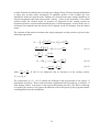
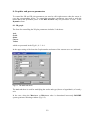
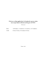
5.2. Principles of electron cooling with circulating electron beam.
The limitations of the electron beam circulating period are determined by the energy exchange
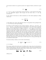
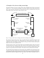
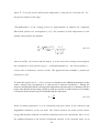
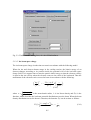
between proton and electron beam due to the cooling process. The principle scheme [7] of the
cooler with circulating electron beam (Fig. 5.1) includes an injector (“electron gun”), storage
ring and electron collector (“electron dump”). The ring has straight section inserted in the
structure of a hadron storage ring, where electron beam merges with proton one and cools it.
Due to interaction between the particles (antiprotons, ions) and electrons the particle
temperature decreases when the electron one increases. The variation of both temperatures in
Maxwellian plasma is described by the equations [7]:
dTp
dt
=
4 2π ηne z 2e 4 LC
γ 2 mM
34
⋅
Tp − Te
 Tp Te 
 + 
M m


3/ 2
;
(5.4)
Np
dT p
dt
= − Ne
dTe
,
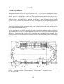
dt
(5.5)
where Tp , Te are the particle and electron temperatures in the particle rest frame, m and M
their masses, Np , Ne – the particle numbers in the rings, η is the ratio of the cooling section
length to the circumference of the particle ring, LC – Coulomb logarithm, ne – the electron
density, t – current time in Laboratory reference frame. The particle temperature in a cooler
with single pass electron beam (and with Maxwellian velocity distribution!) decreases in
accordance with the 1st equation, where Te = const.
Therefore electron temperature in cooling process increase very fast and electron beam is to
be renewed after electrons have got a significant temperature.
For typical parameters of the cooler the number of circulating electrons Ne is comparable with
that one of the particles Np circulating in COSY.
Proton (ion) Ring
p
p
ELECTRON
Dump
e
ELECTRON GUN
(Injector)
Inflector
Infle
ctor
Fig. 5.1. Principle Scheme of Electron Cooler with Circulating Electron Beam
For electron beam with flattened velocity distribution electron beam parameter evolution
during cooling process can be calculated as described in [1]. An example of the electron
temperature variation during circulation is presented for COSY parameters in the Fig. 5.2.
35
1
2
Increase of the cooling time
Fig. 5.2. Evolution of the transverse (1) and longitudinal (2) electron beam temperature during
circulation. Proton beam energy is 1 GeV, proton number is 1011, initial transverse electron
temperature is 300 meV, longitudinal – 50 meV, electron beam radius is 0.5 cm, current –
0.5 A, electron ring circumference is 20 m, magnetic field is 1.2 kG, cooling section length –
1.4 m.
9
8
7
6
5
4
3
2
1
0
2
1
1
10
100
1000
10000
Circulation period, msec
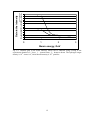
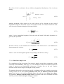
Fig. 5.3. Ratio of the characteristic cooling time of transverse degree of freedom providing by
the cooling system with circulating electron beam to single pass one. Proton beam energy is
2.7 GeV (1) and 1 GeV (2), proton number is 1011, initial transverse electron temperature is
300 meV, longitudinal – 50 meV, electron beam radius is 0.5 cm, current – 0.5 A, electron
ring circumference is 20 m, magnetic field is 1.2 kG, cooling section length – 1.4 m.
The limitation of the circulation period is stronger at low beam energy. In the Fig. 5.3 the
dependence of the cooling time on circulating period is presented at proton beam energy of
1 GeV and 2.7 GeV.
36
At circulation period shorter than 100 msec efficiency of the cooling system with circulating
beam is practically the same as the single pass one (at minimum energy increase of the
cooling time is less than two times). The cooling efficiency decreases during the circulation
and after the period of time longer than approximately a few seconds further circulation of
electrons does not influence practically on the proton beam parameters.
The circumference of the electron ring determines the total number of electrons and as a result
the thermo capacity of the electron beam. In principle the electron beam circumference is to
be as long as possible. The ring circumference of 20 meters is the minimum value, which
permits to install in the ring injection and extraction systems, helical quadrupole lens for
electron focusing and betatron yoke (if it is necessary).
The electron cooling system parameters determined by the requirements of beam
magnetization and cooling efficiency are listed in the Table 5.1 and further calculations are
performed at these parameters.
Table 5.1. General parameters of the electron cooling system with circulating electron beam
Electron ring circumference, m
20
Magnetic field, kG
1 – 1.5
Electron beam radius, cm
0.5
Maximum electron current, A
0.5
Effective length of the cooling section, m
1.4
Circulation period, msec
100 – 1000
Transverse electron temperature, meV
300 – 1000
Longitudinal electron temperature, meV
50 – 100
5.3. Storage ring with longitudinal magnetic field.
At electron energy of 10 MeV and higher usual strong focusing ring can be used for storage of
electrons. In the case of low electron energy the storage ring with longitudinal magnetic field
has some advantage (like electron magnetization) and provides a stable motion of circulating
electrons. Such electron ring can be used simultaneously for preliminary acceleration of
electrons. Then the injector delivers electrons of rather low energy. So called “modified
betatron” is one of possible schemes of the storage ring with cooling electron beam.
Combination of the ring with an injector provides an added bonus.
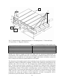
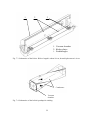
5.3.1 Particle dynamics in the ring with longitudinal magnetic field
Focusing system of the ring consists of straight and toroidal solenoids connected together as a
racetrack. To form a closed orbit for a circulating particle the helical quadrupole winding is
used. In the cooling section the quadrupole field is absent to avoid distortion of the cooling
process. The helical winding can be placed in the straight section opposite to the cooling one.
Due to presence of the longitudinal and helical quadrupole magnetic fields the particle motion
in the horizontal and vertical plane are strongly coupled. When the number of the spiral
winding steps in the focusing section is integer the particle motion in the first approximation
consists of two independent modes [8]:
37
a) fast Larmor rotation of every particle around "own" magnetic field line, which tune is equal
to:
Q fast ≈
C
,
2πρ
(5.6)
ρ = ν / ω B , ω B = eB / γmc is the electron cyclotron frequency, ρ is the electron Larmor radius,
B is the longitudinal magnetic field averaged over the closed orbit, C is the ring
circumference;
b) slow rotation of the beam as a whole around the axis of the helical quadrupole winding
with the tune
2
Qslow
G L
≈ 
,
 B  2k
(5.7)
L is the length of the sections with quadrupole field, G is the gradient of the quadrupole field,
k = 2π/h, h is the step of the spiral winding.
For instance at typical parameters of the focusing system B = 1000 G, G = 20 G/cm, h = 60
cm, L = 120 cm, C = 20 m and at electron energy of 500 keV the working point corresponds
to Qfast = 109.4 (at maximum beam energy of 1.5 MeV Qfast = 49.1), Qslow = 0.24. In this case
dispersion in the cooling section is relatively small: Dx = 10 cm, ellipticity of the electron
beam cross section in the cooling section is less than 1%, i.e. circulating beam in the cooling
section has round shape. Angular spread of the electron beam due to action of the helical
quadrupole field can be reduced to the value less than 1 mrad by adiabatic variation of the
gradient value at the entrance and at the exit of the quadrupole field region. Calculation of the
ring lattice functions and beam parameters in the cooling section are provided numerically
and the algorithm and computer code elaborated in JINR for this aim are described in [9].
Detailed design of the electron ring optics and accurate choice of the working point in the
total range of electron energy can be a topic of further steps of the cooling system design and
are not included in this report.
The motion stability conditions can be written as the following:
Q fast ≠
n
k
, Q slow ≠ , Q fast ± Qslow ≠ l
2
2
(5.8)
n, k, l are integer.
The resonant condition for the fast mode of oscillation (due to large value of its chromaticity)
limits a dynamic aperture of the ring on momentum deviation. The particle momentum spread
can not exceed the distance between nearest integer and half integer resonances. This value
can be estimated by the following expressions:
∆Q fast
 ∆p 
1
∆ρ
 , ∆Q fast ≤ ,
(5.9)
=−
= −
Q fast
ρ
p
4
 max

which gives us
38
 ∆p 
1

~
σ 0 = 
 p  max 4Q fast
.
(5.10)
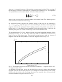
Fig. 5.4 presents the dynamic aperture value at the ring circumference of 20 m. Width and
power of resonances are determined by the errors of the focusing fields. Fast crossing of high
order resonance leads to increase of the beam transverse temperature only. However, during a
long circulation period the stability conditions (5.8) have to be satisfied to keep a good beam
quality even at small instability increment.
At minimum electron beam energy and magnetic field of 1 – 1.5 kG the value of the ring
dynamic aperture (Fig. 5.4.) is approximately equal to 2⋅10-3 and such a value of the electron
beam momentum spread has to be provided by the system of the electron beam acceleration.
At maximum electron beam energy this limitation is not so strong.
σ0
0.015
0.01
2
0)
0.005
1
0
0
500
1000
1500
2000
B
B, G
Fig. 5.4. Dynamic aperture on momentum deviation as function of longitudinal magnetic
field, 1 – beam energy is 500 keV, 2 – beam energy is 1.5 MeV.
In principle, the maximum permitted value of momentum spread limits the circulating beam
current because the momentum shift between particles at the axis and at the beam radius
produced by the beam space charge has not to exceed (∆p / p )max . The shift in electron
momentum due to electron beam space charge is equal to
∆p
eI
= (1 − η n ) 3
p
β γme c 3
,
(5.11)
where ηn is neutralisation factor. Correspondingly, the maximum current of electron beam is
limited by the value
39
I≤
β 3 γm e c 2 σ 0
(1 − η n )e
.
(5.12)
However, even at zero neutralisation factor this condition practically does not limit a possible
value of the beam current up to magnetic field value of several kG (Fig. 5.5).
More serious limitation of the circulating beam current is determined by the threshold of the
microwave instability and it is discussed in the next chapter.
Imax, A
50
40
30
)
20
10
0
1000
2000
3000
4000
5000
B
B, G
Fig. 5.5. Upper limit of the circulating beam current determined by momentum shift due to its
space charge. Beam energy is 500 keV, neutralisation factor is equal to zero.
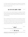
5.3.2 Current limitation due to microwave instability
At given maximum value of the momentum spread the longitudinal microwave instability
limits the intensity of the circulating beam. Dynamics of longitudinal motion in the LEPTA is
the same as in a standard strong focusing ring, and therefore we can use the usual criterion for
longitudinal stability of the electron beam, which can be written as follows [10]:
I ≤ 4 Flong
mc 2 β 2γ η
e Zn / n
σ 2f ,
(5.13)
σf is a spread in momentum deviation (half width on half height). Zn is a longitudinal coupling
impedance of the beam for a mode with number n. Factor Flong takes into account the real
shape of the stability diagram. In standard Keil-Schnel criterium Flong = 1. However, when
beam energy is less than critical one and momentum distribution function has a long "tails"
Flong value can be significantly larger than unit. In this case with a good accuracy we can
write:
Flong ≅ σ 02 / 2σ 2f ,
40
(5.14)
where σ0 is a dynamical aperture of the machine on momentum deviation. If the crossing of
the half-integer resonance is impossible σ0 is limited by the condition (5.10). The impedance
for cylindrical beam and vacuum chamber is described with the formula:
Zn
377 
b
=
 1 + 2 ln  ,
2
n
a
2 βγ 
(5.15)
where b and a are the radii of vacuum chamber and electron beam. This formula gives us
about 250 Ohms at minimum beam energy.
For described focusing structure the transition energy of the ring can be estimated as
γ tr2 ≅ ± Q fast Q slow [8]. The sign of γtr2 is determined by the directions of the longitudinal
magnetic field and the qudrupole helical winding rotation, what permits to us choose the
regime with η > 0 (no negative mass instability) in the total energy range. In this case the
instability takes place due to finite conductivity of the vacuum chamber walls.
The threshold current (5.13) as a function of beam energy and longitudinal magnetic field is
presented in the Fig. 5.6, the tune value of the slow mode of oscillations was chosen to be
equal 0.2 in the total energy range. The threshold current decreases with the increase of
magnetic field value due to dependence of σ0 on the magnetic field (see Fig. 5.4).
I, A
100
1
2
10
1
400
600
800
1000
1200
1400
1600
Beam energy, keV
Fig 5.6. Threshold electron beam current of microwave instability: 1 – magnetic field is 1 kG,
2 – magnetic field is 2 kG.
At minimum electron beam energy the threshold beam current is higher than maximum
designed value only by two times, however, even taking into account decrease of the cooling
efficiency for the system with circulating electron beam, required value of electron beam
current at minimum energy does not exceed 0.3 A.
41
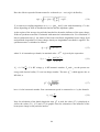
5.3.3. Transverse-longitudinal relaxation of electron beam
In the magnetised electron beam intrabeam scattering is substantially suppressed by
longitudinal magnetic field. Characteristic time of the temperature growth rate can be
estimated by the following empirical expression [11]:
1
τ relax
1 dT|| 2πre2 ne mc 3 LC
=
≈
T|| dt
T||
mc 2 −2.8 / ρn1e / 3
,
e
T⊥
(5.16)
where re is the electron classical electron radius, Lc ~ 10 is the Coulomb logarithm, ne is the
beam density, ρ = 2mc 2T⊥ / eB is the particle Larmor radius in the longitudinal magnetic
field B. Exponential term in (5.16) leads to strong dependence of the relaxation characteristic
time on the temperature of transverse degree of freedom and on the beam current (Fig. 5.7).
At electron beam current of 0.1 A the magnetic field value of 1.5 kG seems to be big enough
to suppress intrabeam scattering of the electron beam during the period required for beam
circulation. At maximum electron beam current the relaxation time is less than circulation
period by about three orders of magnitude. It means that this process has to be taken into
account in estimations of the cooling system efficiency.
The formula (5.16) describing the electron beam relaxation is half-empirical one and due to
importance of this process for cooling system with circulating electron beam has to be
carefully tested with the real installation. The process of the transverse – longitudinal
relaxation in the cooling system with circulating electron beam will be experimentally
investigated at LEPTA ring (see chapter 7).
42
Relaxation time, sec
1
3
a)
0.1
2
0.01
1
0.001
1 10
4
0.2
0.3
0.4
0.5
0.6
0.7
0.8
0.9
1
0.01
b)
3
0.001
)
)
2
)
1 10
4
1
1 10
5
0.2
0.3
0.4
0.5
0.6
0.7
0.8
0.9
1
Transverse temperature, eV
Fig. 5.7. Characteristic time of the transverse-longitudinal relaxation of the electron beam,
magnetic field is 1 kG (1), 1.5 kG (2), 2 kG (3), longitudinal temperature is 50 meV, electron
beam current is 0.1 (a) and 0.5 A (b).
5.4. Electron cooling with circulating electron beam in experiments with internal target
In experiments with internal target additional limit appears for the electron beam circulation
period. It is connected with the coherent energy losses of the ion beam due to interaction with
the target. Due to energy exchange between the ion beam and circulating electron one the
beam velocities in the cooling section are the same. Correspondingly, the coherent energy
variation of the electron and ion beams during the circulation period are connected in
accordance with the relation:
43
 ∆E 
 ∆E 

 =
 .
 E  e  E i
(5.17)
During the circulation period the energies of the ion and electron beams have to be inside the
dynamic apertures on momentum deviation of corresponding ring. The dynamic aperture on
momentum deviation of the electron ring with longitudinal magnetic field (σ0 formula 5.10) is
less than that one of the ion ring. Coherent momentum shift of the electron beam can be
calculated as the following:
δp 1 ∆E Tcirc
=
p 2 E Trev
,
(5.18)
where ∆E is the ion energy loss after crossing the target (formula 1.2), E is the ion energy and
Tcirc is the electron beam circulation period. From the condition δp/p ≤ σ0 one can write the
condition for upper limit of the circulation period:
Tcirc ≤ Tmax,1 =
Trev Eρ L
,
2∆EC
(5.19)
where C is the electron ring circumference, ρL is the electron Larmor radius in the
longitudinal magnetic field, Trev is the ion revolution period. The dependencies of the
maximum circulation period of the electron beam on the particle energy and the target density
are presented in the Fig. 5.8. In the total range of the COSY experiment parameters the
circulation period has to be less than about 1 second to avoid a resonance of the electron
beam.
Other limitation connected with this effect is related to distortion of the cooling process after
refresh the electron beam: the coherent momentum shift of the ion beam after circulation
period has to be substantially less than its momentum spread. Only in this case the model
using for cooling process simulation gives correct results for the system with circulating
electron beam. The condition, when the used numerical model is valid for calculation of the
cooling time for the system with circulating electron beam, can be expressed in the following
form:
Tcirc << Tmax, 2 =
2Trev E (∆p / p )i
∆E
.
(5.20)
The momentum spread of the ion beam (∆p/p)i depends on many parameters and can be
varied by about one order of magnitude depending on experiment conditions. In the Fig. 5.9
the coherent energy shift of the proton beam as a function of the circulation period and beam
energy is presented. One can see that at circulation period of about several hundreds of msec
this effect can be ignored at all reasonable ion beam parameters.
44
Circulating period, sec
1 .10
.
3
100
1
10
2
1
3
0.1
15
1 .10
1 .10
Target density, Atoms/cm^2
1 .10
16
17
a)
Circulating period, sec
1 .10
.
3
100
1
10
2
1
3
0.1
0.01
15
1 .10
16
1 .10
Target density, Atoms/cm^2
1 .10
17
b)
Fig. 5.8. Maximum circulating period of the electron beam as function of the target density:
a) proton beam at energy 2700 MeV (1), 1000 MeV (2), 500 MeV (3);
b) deuteron beam at energy 2100 MeV (1), 1000 MeV (2), 500 MeV(3).
1.5 .10
4
Relative energy losses
.
1 .10
4
1
5 .10
5
2
0
0
0.2
0.4
0.6
Circulation period, sec
0.8
1
Fig. 5.9. Relative energy losses of the proton beam at target density of 1016 Atoms/cm2, at
energy 1000 MeV (1) and 2000 MeV (2).
45
5.5. Induction acceleration of the electron beam.
The electron acceleration can be provided using RF linac with further injection into electron
ring or inside the electron ring using low frequency betatron acceleration. In the second case
the energy spread of the accelerated electron beam caused by variations of the acceleration
voltage during revolution period, is equal to [12]:
∆ε = e(
∂V
∂V
τ rev ) inj − e(
τ rev ) fin ,
∂t
∂t
(5.21)
where V is the accelerating voltage, τrev is the electron revolution period. When V=V0sin(ωt)
and initial and final phases of acceleration are symmetrically disposed around the voltage
maximum, this formula gives us
2
∆ε  Cω  1 − βinj
≈
.

 c  βinj β
ε
(5.22)
In this case the acceleration voltage amplitude can be obtained by integration of the motion
equation:
eV 0 =
ε
Cω
,
c 2 β cos ωt inj
(5.23)
where C is the electron ring circumference, βinj, β - initial and average electron velocity in
the units of the speed of light.
Using the existing COSY high voltage power supply for injection one can accelerate electrons
0.5 msec from ε = 100 keV (injection) up to 1.5 MeV. The estimated momentum spread value
caused by the voltage variation is negligible (Table 5.2).
Table 5.2. Parameters of the induction acceleration system
Injection energy, keV
100
Maximum energy, keV
1500
Electron ring circumference, m
20
Frequency of the acceleration voltage variation, kHz
1
Required amplitude of the acceleration voltage, V
500
Beam momentum spread caused by voltage variation
2⋅10-7
During the electron beam acceleration inside the ring with constant value of the longitudinal
magnetic field the working point crosses series of the resonances of the fast mode of
oscillation. The experiments at Modified Betatron Acceleratator in NRL (USA) [13] have
shown that the crossing of the high order resonances does not lead to the particle losses. An
increase of the beam transverse temperature in these experiments was not investigated and we
plan to perform such investigations at LEPTA ring (see chapter 7).
46
6. Principles of the electron cooling system design
All general elements of electron cooling system with circulating electron beam are presented
in the Fig. 6.1. If the electron acceleration is performed with RF electron linac, the betatron
yoke is not necessary and instead of electron gun one needs to install the RF cavity and
debunching system, if necessary to reduce ∆p/p (see [14]).
Electron cooling section
Injection
kicker
Injection
septum
Helical quadrupole
winding
Electron gun
solenoid
Extraction
kicker
Extraction
septum
Betatron
yoke
Collector
Fig. 6.1. Layout of the electron cooling system with circulating electron beam.
The electron beam injection into the ring is provided along the longitudinal magnetic field
with transverse field of septum coils, which displace the electron beam to the vicinity of the
equilibrium orbit at the distance of about diameter of the gun solenoid. Than the kicker plates
displace the beam to the equilibrium orbit.
Inside the septum coil the electron beam drifts in the longitudinal magnetic field of the septum
solenoid and transverse magnetic field of the septum coil. The field of the septum coil has a
zero value at the orbit of circulating beam due to special coil design. Possible design of the
septum coil is presented in the next chapter. The septum coils are operated in the DC mode.
The field of the kicker displaces the electron beam to the equilibrium orbit and after the beam
occupies the total ring circumference the field of the kicker has to be switched off during the
time substantially shorter than revolution period. Drift of the electrons inside the kicker can be
performed by transverse magnetic field or by electric field. When electrostatic kicker is
47
applied the cooling system can be used also in the single pass mode of operation. In this case
both kickers – injection and extraction are used in the DC mode and electron beam is
displaced by injection kicker to the orbit inside the cooling section and after moving through
the cooling section is displaced to extraction septum and to the collector by extraction kicker.
Such a possibility looks like very attractive for COSY – it permits to use electron cooling
system at injection energy in the single pass regime with existing electron gun and its power
supply system. The example of the electrostatic kicker design is presented in the next chapter.
In the case of induction acceleration of the electron beam the existing COSY electron cooling
system can be upgraded to medium energy electron cooling system by installation of several
new solenoids and betatron yoke for electron acceleration. Two of the new solenoids (septum
solenoids) are to be placed vertically above the existing toroidal solenoids. In each of these
solenoids the coils of magnetic septum and electrostatic kicker are placed. Existing electron
gun and collector with their solenoids are placed above these two new septum solenoids. To
form a closed orbit for electron beam two toroidal and straight solenoids are connected with
the septum solenoids. In the straight solenoid (which is placed opposite to the cooling section)
the betatron yoke and helical quadrupole windings are placed.
In the regime with circulating electron beam the beam from the gun is directed to the closed
orbit by injection septum and kicker plates. When the beam fills total circumference of the
electron ring kicker voltage is switched off. After that beam is accelerated to required energy
with the betatron yoke. Next current pulse applied to the betatron yoke coil decelerates the
circulating electron beam and after deceleration the electron beam is extracted to the collector
by the pulse applied to the extraction kicker.
The cooling system with induction acceleration has a lower cost in comparison with RF
acceleration, but general problem of this system is beam quality degradation after crossing of
number of resonances. This problem as well as optimisation of injection system can be
experimentally investigated at LEPTA ring.
48
7. Program of experiments at LEPTA
7.1. LEPTA parameters
The general aim of the LEPTA ring construction (Fig. 7.1) is to provide storing low energy
positrons, electron cooling of positrons and generation of the directed flux of positronium
atoms. However at design study of the ring all the parameters were chosen such that we have
a possibility to test beam parameters required for electron cooling system with circulating
electron beam. The parameters of the ring in the mode with circulating electron beam
(Table 7.1) are closed to the parameters of COSY cooling system and designed parameters of
the betatron yoke cover the total energy range of the circulating beam required for COSY.
Adjustment of the injection and extraction system, investigations of an influence of the helical
quadrupole winding will be performed during ring commissioning using optic method of the
beam temperature measurement [3].
At the first stage of the LEPTA operation the study of the beam dynamics will be performed
at the beam energy of 10 keV and variation of the beam energy will be provided using small
RF cavity. Final test of the system will be performed after installation of the betatron yoke
and it presumes the electron beam acceleration and test of the beam temperature at maximum
required energy.
Fig 7.1. The assembly drawing of the LEPTA: 1 - extraction kicker, 2 - septum, 3 - injection
kicker, 4 - toroidal sections, 5 - betatron core, 6 - electron gun, 7 - electron collector,
8 - cooling section.
49
Table 7.1. General parameters of the LEPTA.
Ring parameters
Circumference, m
Longitudinal magnetic field, G
Major radius of the toroids, m
Bending magnetic field, G
Gradient of the quadrupole magnetic field, G/cm
Electron beam radius, cm
Residual gas pressure, Torr
Electron beam parameters
At injection
Energy, keV
10
Current, A
0.1
Revolution period, nsec
300
Acceleration cycle
Induction voltage amplitude, V
Repetition frequency, Hz
Cycle duration, msec
18.28
1000
1.45
1.75 – 124
10 – 15
1.0
10-10
After acceleration
4360
0.5
60
50
1
10
7.2. Preliminary program of the experiments.
General problems which have to be experimentally investigated before design of the full scale
electron cooling system with circulating electron beam are the following:
- beam parameter distortion during injection,
- variation of the longitudinal beam temperature due to transverse-longitudinal relaxation,
- beam parameter distortion after crossing the resonances of the fast mode of oscillation.
The aim of the investigations is the final choice of the magnetic field value and the optimal
position of the working point of circulating beam in the total range of the beam energy,
accurate measurements of the maximum beam current which can circulate in the ring without
loss the quality during required period of time. These experiments will be performed at the
special test bench during the LEPTA assembling and with circulating electron beam during
the ring commissioning.
7.2.1. Tuning of injection system and helical quadrupole winding
Injection system of the ring consists of magnetic septum (Fig. 7.2, Table 7.2) and electrostatic
kicker (Fig. 7.3). Variation of the angle of the electron beam trajectory at the entrance and at
the exit of the septum and kicker is about 15 mrad and only a resonance optics of these
elements permits to keep electron beam quality after injection. In this case the integer number
of the electron larmor rotations has to take plase at the length of the kicker and septum.
Calculate of the effective length of the septum and kicker coils accurately is a complicated
numerical problem and these values will be measured experimentally using optic method of
the electron transverse temperature measurements.
50
3
4
5
120
1
2
752
2560
Fig.7.2. Septum design.1 -Beam from the gun, 2 - Circulating beam, 3 - Extracted beam,
4 -Current lines, 5 - Magnetic field lines.
Magnetic field value, G
Current, A
Number of turns
Conductor cross-section, mm
Beam displacement, mm
Table 7.2. General parameters of the septum coils.
120
1600
6
4 x 12
300
Initially the effective lengths of both coil fields will be measured independently by
measurement of the magnetic field value corresponding to minimum distortion of the beam
parameters after crossing the coil. After that the length of the kicker coil will be corrected to
have an integer ratio between septum and kicker coil lengths.
The distortion of the angular spread of the circulating electron beam after crossing the helical
quadrupole winding is minimised by adiabatic variation of the quadrupole field gradient at the
entrance and at the exit of the coil. The designed and constructed helical quadrupole coil
(Fig. 7.4) has in each crossection a geometry of "Panofsky lens" which provides a maximum
linearity of the field. The gradient variation at the enetrance and exit of the coil is provided by
corresponding variation of the number of winding turns. Accurate calculation of the particle
dynamics in the coil is practically impossible due to difficulties in measurements of the fringe
fields, and test of the coil and (if it would be necessary) correction of its design will be
performed also using optic method of beam diagnostics. All these investigations will be
performed at special test bench, which is under construction now.
51
1
3
2
1. Vacuum chamber
2. Kicker plates
3. Feedthroughs
Fig. 7.3. Schematics of the kicker. Kicker length is about 90 cm, beam displacement is 6 cm.
I
I
Conductors
Vacuum
chamber
Fig. 7.4. Schematics of the helical quadrupole winding.
52
7.2.2. Study of the circulating beam dynamics
Stability diagram in the vicinity of the working point at injection energy of 10 keV is
presented schematically in Fig 7.5. The most dangerous resonances are the integer (342 and
343) and half integer (342.5) ones of the fast mode of oscillations, the half integer and 1/3
nonlinear of slow mode of oscillations and the coupling resonance of the modes
Q fast + Qslow = 342 . Nonlinear resonances of the fast mode of oscillations have very high
order and estimations show that they practically do not influence on beam parameters.
An accurate calculations of the position of the resonances and increments in their centre were
performed using especially elaborated computer code BETATRON. Power of nonlinear
resonance of slow mode of oscillations was calculated using averaging method. The nonlinear
resonance appears due to sextupole component of the longitudinal magnetic field in the
toroidal sections and leads to variation in time of the motion invariant corresponding to the
slow mode of oscillation. Due to coupling between horizontal and vertical degrees of freedom
the variation of slow invariant produces variation in time of the beam cross-section. In
experiment the power of the resonance can be estimated by measurements of the frequency of
beam cross-section variation.
Real width of the linear and coupling resonance is determined by the errors of the focusing
fields. In the case of focusing by longitudinal magnetic field the errors can not to be
calculated through the errors in the position of the focusing elements. The errors of the
focusing field appear due to those in the solenoid winding and can be evaluated only by
measurements of the real field distribution in each section of the solenoid. However the field
measurements has to be performed in the position of the closed orbit which is known with
accuracy of about a few millimetres.
Qslow
Coupling resonance
0.5
1/3
Qfast
342.5
343
342
Fig 7.5. Stability diagram in the vicinity of the working point at beam energy of 10 keV and
magnetic field value of 400 G.
53
Thus the dynamic behaviour of the ring can be investigated only experimentally. And such an
investigation is of great importance for proposed cooling system. The width and power of the
fast mode resonances in real structure are the key parameters in the problem of betatron
acceleration of circulating beam. A possibility of the resonance crossing and beam parameters
distortion in the resonance vicinity will determine the choice of acceleration regime. In the
case of electron beam acceleration with RF accelerator the dynamics investigation will
determine the requirements to the momentum spread of injected electron beam.
The tune of the slow mode of oscillation can be measured using pick up electrodes. The
frequency of the slow oscillations at beam energy of 10 keV is about 700 kHz and
corresponds to coherent oscillations of circulating beam. The tune of the fast mode of
oscillations can not to be measured directly (characteristic value of the frequency of the fast
mode of the betatron oscillations is about 1 GHz, and the signals produced by each particle on
pick-up electrodes are incoherent.) Its measurements we plan to perform by displacement of
the beam energy to the region of the coupling resonance which leads to increase of the
amplitude of the slow mode. For this aim small RF cavity will be installed in the ring.
In order to test beam parameters variation after the resonance crossing the beam will be
extracted from the ring and directed to the optic diagnostics for the beam temperature
measurement.
The longitudinal temperature of the circulating electron beam will be measured using
Schottky diagnostics. This permits to measure growth rate of the longitudinal temperature due
to transverse-longitudinal relaxation, which is impossible in the case of single pass electron
beam of a traditional electron cooling system. Experimental study of the relaxation process
allows finding the limit of the maximum value of the electron beam current in the electron
cooling devices with circulating electron beam.
54
Summary
1. Role of the cooling in experiments with internal targets
The beam energy and required target density in experiments with internal targets is
determined by physical problem to be investigated. Investigations of nature of a0-mesons are
to be performed at maximum proton beam energy, required level of the luminosity is
1033 cm-2⋅sec-1 and higher. This experiment can be provide using a pellet target.
Measurements of the deuteron break-up, ω, η, K mesons production are performed in the
wide energy range from 1 GeV to about 2 GeV, and with all the types of the ANKE targets.
The effective density of the hydrogen cluster beam target, achieved in the experiment at
January/February 2001, is about 2⋅1015 Atoms/cm2. Expected areal density of the gas storage
cell is 1014 - 1015 Atoms/cm2. Effective density of the frozen pellet target is expected to be
between 3⋅1014 and 2⋅1016 Atoms/cm2 at beam emittance of 1 π⋅mm⋅mrad.
In the experiments with the internal target the upper limit of the circulating beam life time
(and, as a result, the experiment duration) is determined by single scattering on large angles
with the target atoms. At the target density below 1015 Atoms/cm2 the beam life time and
characteristic times of the emittance growth due to interaction with the target are longer than
one hour and experiment can be performed without cooling. At the effective target density
over than approximately 2⋅1016 Atoms/cm2 the beam life time is shorter than expected cooling
times at realistic parameters of the cooling system. In this case cooling cannot effect on the
beam parameters effectively.
The range of the target density from 1015 to 2⋅1016 Atoms/cm2, in which cooling can be used
for luminosity preservation, covers parameters of all types of the ANKE target practically.
Only in the experiments with solid target the beam life time is so short that luminosity
preservation using cooling seems to be unrealistic. The difference between the hydrogen and
deuterium targets is not substantial because of the general processes which influences on the
beam parameters are determined by interaction with the electrons of the target atoms.
In this report the possibility of the cooling application was investigated in two ranges of the
target density: long term experiment (up to 1 hour) at the target density of 1015 Atoms/cm2
and short term experiment (about 5 minutes) at the target density of 1016 Atoms/cm2.
In the experiment with gas storage cell target, when the target dimensions coincide with the
aperture of the vacuum chamber, the role of the beam cooling is to reduce the particle losses
due to aperture limitation by suppression of the emittance growth. Maximum achievable gain
in the experiment luminosity is determined by the relation between the beam life time and
time of the emittance growth up to acceptance.
For proton beam at the target density of 1015 Atoms/cm2 after one hour of experiment
maximum possible gain in the beam intensity is more than two times at the energy below 2
GeV (up to one order of magnitude at 1 GeV), and about 50% at energy of 2.7 GeV.
For circulating deuteron beam the gain in intensity of about 50% can be obtained at energy of
2.11 GeV (which corresponds to the maximum magnetic rigidity). At intermediate energies
the gain in the beam intensity is determined by suppression of the intrabeam scattering and for
55
deuteron beam is about two times less than the proton one, however at energy of 1 GeV the
possible gain in the luminosity for deuteron beam is about 5 times.
Similar dependence on the particle energy takes place at the target density of 1016 Atoms/cm2,
but maximum expected gain in the beam intensity after five minutes of experiment is about
1.5 times higher.
The energy dependence of the maximum gain in the experiment luminosity is explained by
the input of the intrabeam scattering into emittance growth. The role of this process fast
decreases with the energy increase and at maximum beam energy emittance growth is
determined by the single scattering with the target atoms mainly. Thus, the potential
efficiency of a beam cooling increases with increase of the beam intensity and decreases with
increase of the beam energy.
In the experiment with cluster beam target additional gain in the luminosity can be obtained
due to the target dimension in the horizontal plane is 5 mm, which is less than beam
dimension corresponded to acceptance limitation. Stabilisation of the horizontal beam
dimension during experiment can give additional gain in the luminosity of about 50%.
In the experiment with the pellet target the luminosity is inversely proportional to the
circulating beam cross section because of the beam cross section always larger than pellet
one. In this case the beam cooling can provide increase the luminosity by several times. When
the cooling prevails on the heating effects one can realise the regime with constant luminosity
during the time of experiment via compensation of the particle losses by corresponding
decrease of the beam emittance.
Thus, in the experiments with the gas jet and cluster beam targets the experiment duration can
be about one hour without substantial loss of the luminosity and cooling application can give
gain in the luminosity from 50% to 5 - 10 times at energy from 1 to 2.7 GeV. In the
experiment with the pellet target the experiment duration can be about 5 minutes and cooling
application can give a gain in the luminosity of about 2-3 times in the total range of the beam
energy.
2. The possibility of the existing stochastic cooling system application
The effectiveness of the stochastic cooling strongly depends on the ion beam intensity. In this
report the possibilities of the stochastic cooling were investigated under assumption that one
of the chains is used for cooling of the horizontal degree of freedom, other one - for
longitudinal. In this case the stochastic cooling system can be used for luminosity
preservation at the target areal density of about 1015 Atoms/cm2 up to ion beam intensity of
about 2-3⋅1010 particles. Maximum efficiency of the stochastic cooling corresponds to the
maximum beam energy (due to dependence of the mixing factor on the off-momentum
factor). The gain in the luminosity is close to the theoretical value and in the experiment with
the gas jet target is about 20 – 50%, in the experiment with cluster beam target this value can
be higher by about 1.5 times due to stabilisation of the horizontal beam dimension.
At the beam intensity of 1011 particles, which corresponds to expected value with new COSY
injection system, or at high target density the existing stochastic cooling system is not
powerful enough to expect a substantial effect from its application in the experiment with
internal target.
56
3. The possibility of an electron cooling application
Electron cooling system at realistic parameters of the electron beam stabilises the parameters
of the intensive (up to 1011 particles) ion beam at the target areal density of 1015 Atoms/cm2 in
the total energy range required for experiments. Maximum gain in the luminosity corresponds
to the minimum beam energy. In the experiment with gas jet target for the proton beam
expected gain in the luminosity after one hour of experiment is 2 – 3 times at 1 GeV and
decrease to the value of 20 – 50% at 2.7 GeV. For deuteron beam expected gain in the
luminosity is about 2 times at energy of 1 GeV and decreases to 50% at 2.11 GeV. In the
experiment with cluster beam target additional gain in the luminosity can be obtained due to
stabilisation of the horizontal beam dimension and its value is about 1.5 times.
In the experiment with the pellet target maximum gain in the luminosity is expected at
minimum beam energy. In this case the experiment duration can be about 5 minutes and gain
in the integral luminosity is 2 – 4 times depending on the pellet diameter. The expected
average luminosity value exceeds 1033 cm-2sec-1. At these parameters one can realise the
regime with permanent luminosity during the time of experiment via compensation of the
particle losses by corresponding decrease of the beam emittance.
At maximum proton beam energy of 2.7 GeV the electron cooling compensates the beam
heating due to interaction with target only at pellet diameter of 40 –50 µm, which corresponds
to the luminosity value of 3 - 5⋅1033 cm-2⋅sec-1. At maximum pellet diameter the electron
cooling does not suppress the beam heating, but it can be used for initial preparation of the
beam parameters before the target switching on. In combination with the optimum experiment
strategy it can give a gain in the integral luminosity of about 20%. It should be noted that all
the simulations in this report were performed under assumption that each moment of time one
pellet is in the beam. In the case of low frequency of the pellet production the effective target
density has to be calculated taking into account the duty factor. Final conclusion can be
expressed as follows: in the experiment with the pellet target at maximum proton beam
energy an electron cooling gives substantial gain in the luminosity up to the luminosity level
of about 5⋅1033 cm-2⋅sec-1.
For deuteron beam an electron cooling can be effectively used in the total energy range and at
beam energy of 2.11 GeV and maximum target density the gain in the integral luminosity
after five minutes of experiment is about 50% and it increases to several times at less energy
or target density.
4. Electron cooling system with circulating electron beam
There are two possible design of new COSY cooling system:
- Traditional configuration of cooling system + HV accelerator,
- Cooling system with circulating electron beam.
Traditional configuration of the cooling system can provide electron beam at low transverse
and longitudinal temperature, and the results of numerical simulations demonstrate its ability
for ion beam parameters stabilisation.
57
Electron cooling system with circulating electron beam has substantially low cost, but in such
a system the electron beam quality is expected to be rather less than in the HV system. The
electron beam quality is determined by a method of the beam acceleration, stability of
electron motion in the electron storage ring, number of electrons and the ring circumference.
General attention of this report was attracted to the possibility of the electron cooling system
with circulating electron beam. In the electron energy range from 0.5 to 1.4 MeV only a
longitudinal magnetic field can provide strong focusing of an intensive electron beam.
General parameters of the electron ring with longitudinal magnetic field can be the following:
magnetic field value is 1 – 1.5 kG, the ring circumference is about 20 m, electron beam radius
is 0.5 mm, maximum current value is 0.5 A. The electron beam acceleration can be provided
using RF electron linac or by induction acceleration of the electrons in the ring. The induction
acceleration is more attractive from the side of the momentum spread of accelerated beam and
installation cost, but it did not tested experimentally. The proposed design of the injection
system of the electron ring permits to perform two modes of operation: with the single pass
electron beam at injection energy and with the circulating electron beam at the energy of
experiment. Some elements of the existing COSY electron cooling system can be used in the
new cooling device.
General problems of the proposed cooling system are the following:
- distortion of the electron beam parameters during its injection into the ring,
- motion stability of the electron beam during circulation,
- heating of the electron beam due to its interaction with the cooled ion one,
- coherent energy losses of both beams – ion and electron – due to interaction of the ion beam
with the target and energy exchange between beams,
- heating of the longitudinal degree of freedom of the electron beam due to intrabeam
scattering.
In the case of induction acceleration of the electron beam more serious problem is to avoid
beam heating during crossing of resonances of transverse particle motion.
The period of the electron beam circulation is limited by the heating due to interaction with
the ion beam. When the circulation period is about 0.1 second the efficiency of proposed
system is the same as one of the traditional electron cooling system. More serious limitation
can appear due to transverse-longitudinal relaxation in the electron beam. This problem as
well as the stability of the electron motion and electron beam distortion during injection
requires experimental investigations. They can be performed at LEPTA installation, which
construction is in the final stage in JINR. We plan to begin the experimental program next
year and expected term of its completion is two years.
The cost of the cooling system with circulating electron beam estimated using the experience
of construction of analogous system in JINR can lies between 1 and 1.5 M$.
Conclusion and recommendations
In the experiments with gas storage cell and cluster beam targets an electron cooling system
can be effectively used for the luminosity preservation when the experiment duration is of the
order of 1 hour. In this case expected gain in the luminosity is about 2 – 3 times at minimum
and intermediate beam energy. At maximum beam energy the effect of cooling application
decreases and at the target density below 1015 Atoms/cm2 the experiment can be performed
58
without luminosity loss during long period of time without cooling. Electron cooling
stabilises the beam parameters in the total energy rang and transverse dimensions of the ion
beam during experiment can be 2 – 3 times less than in the case without cooling. This permits
to decrease the aperture of the gas storage cell in order to increase the target density.
In the experiment with the pellet target at maximum proton beam energy an electron cooling
gives substantial gain in the luminosity up to the luminosity level of about 5⋅1033 cm-2⋅sec-1
and at experiment duration up to five minutes. Using of an electron cooling system one can
realise the regime with permanent luminosity during the time of experiment via compensation
of the particle losses by corresponding decrease of the beam emittance. An electron cooling
application gives a possibility to optimise the ion beam parameters and experiment duration in
order to obtain maximum integral luminosity taking into account the time of the beam storage
and acceleration.
The proposed scheme of the electron cooling system with circulating electron beam permits to
provide the effective ion beam cooling in the total energy range and in the single pass mode of
operation the beam cooling during storage process at injection energy. However the technical
design of such a system can not be performed without an experimental test of its general
elements.
59
References
1. Electron cooling application for luminosity preservation in an experiment with internal
targets at COSY. Interim report, Dubna, 2001.
2. I.Meshkov, A. Sidorin, Electron cooling system with circulating electron beam. Workshop
on Medium Energy Electron Cooling, Novosibirsk,1997, p. 183, G. Jackson, Modified
Betatron Approach to Electron Cooling. Workshop on Medium Energy Electron Cooling,
Novosibirsk,1997, p.171.
3. V.Golubev, I.Meshkov, V.Polyakov, I.Seleznev, A.Smirnov, E.Syresin ,The proceeding of
the Workshop on Beam Cooling and Related Topics, CERN 94- 03, 26 April 1994
4. F. Hinterberger, D.Prasuhn, Analysis of internal target effects in light ion storage ring, NIM
A 279(1989), 413-422
5. D.Anderson at al., The development of a prototype multi-MeV electron cooling system,
T.Ellison at al., Multi-MeV electron cooling – a tool for increasing the performance of high
energy colliders?, Fifth Annual International Industrial Symposium on the Super Collider, 6-8
may, 1993, San Francisco, California.
6. I.N.Meshkov, Fiz. Elem. Chastits At. Yadra 25 (1994) 1487 [Engl. transl.
Phys.Part.Nucl.25 (6) (1994) 631], I.Meshkov, preprint RIKEN-AF-AC-2, January 1997.
7. Yu.V.Korotaev, I.N.Meshkov, S.V.Mironov, A.O.Sidorin, E. Syresin “The Modified
Betatron Prototype Dedicated to Electron Cooling”, 6th European Particle Accelerator
Conference, Stockholm, 22-26 June, 1998., M.Chelnokov, V.Kalinichenko, Yu.Korotaev,
I.Meshkov, S.Mironov, A.Petrov, I.Sedykh, A.Sidorin, A.Smirnov, E.Syresin, I.Titkova,
G.Trubnikov, Modified Betatron Prototype Dedicated to Electron Cooling with Circulating
Electron Beam, Proc. HEACC’98, Dubna, 1999, p. 413, I.Meshkov, Electron cooling with
circulating electron beam in GeV energy range, NIM A 441(2000), p.255.
8. I.Meshkov, A.Sidorin, A.Smirnov, E.Syresin The particle dynamics in the low energy
storage rings with longitudinal magnetic field, 6th European Particle Accelerator Conference,
Stockholm, 1998, p. 1067,
9. I.N.Meshkov, A.O.Sidorin, A.V.Smirnov, E.M.Syresin, G.V.Trubnikov , “Betatron
program for simulation of particle dynamics in storage ring with strong coupling of
transverse coordinates”, proceedings of ICAP2000, Darmstadt, to be published in Phys.Rev.
(Accelerators & Beams)
10. I.Meshkov, A.Smirnov, A.Sidorin, E.Syresin, E.Mustafin, P.Zenkevich, The Stability of
the Circulating Electron Beam in the Electron Cooling System Based on the Modified
Betatron, Proc. HEACC’98, Dubna, 1999, p.416.
11. A.V.Aleksandrov, N.S.Dikansky, N.Ch.Kot, V.I.Kudelainen, V.A.Lebedev,
P.V.Logachev, Proc. Workshop on Electron Cooling and New Cooling Techniques, Legnaro,
1990 (World Scientufic, 1991) p. 279
12. JINR electron cooling group, "The report of the Designing of the Modified Betatron
Prototype", JINR, Dubna, 1997.
13. C.Kapetanakos, et.al., The Naval Research Laboratory Modified Betatron
Accelerator and Assessment of its Results, Phys. Fluids B 5(7), 1993, p.2295.
14. K.Balewski, et. al., Preliminary Study of Electron Cooling Possibility of Hadronic Beam
at PETRA, 6th European Particle Accelerator Conference, Stockholm, 22-26 June, 1998,
p.1079
60
Annex I
Electron cooling application for luminosity preservation
in an experiment with internal targets at COSY.
Interim report
JINR
I.N.Meshkov, Yu.V.Korotaev, A.L.Petrov, A.O.Sidorin,
A.V.Smirnov, E.M.Syresin, G.V.Trubnikov, S.V.Yakovenko
COSY
H.J.Stein
Dubna, 2001
61
CONTENTS
Abstract
3
Introduction
4
1. General description of the physical model
4
4
5
1.1. Beam emittances and particle number evolution
1.2. Particle losses and emittance calculation in the presence of beam scrapers
2. Heating processes involved into calculations
2.1. The interaction with the target atoms
2.1.1. Description of the COSY internal targets
2.1.2. Emittance growth and beam lifetime
2.1.3. Target parameters calculation
2.2. Intrabeam scattering of the ion beam
2.2.1. Piwinski model
2.2.2. Martini model
2.3. Ion multi scattering on residual gas atoms
2.4. Tune resonances of the ion betatron motion
2.5. External heating
3. Particle losses calculation
3.1. Nuclear scattering on residual gas atoms
3.2. Single scattering on large angles
3.3. Recombination in the electron cooling section
3.4. Other particle losses
7
7
7
8
9
11
11
12
14
15
15
16
16
16
17
17
4.1. Stochastic cooling
4.1.1 Transverse cooling time
4.1.2 Longitudinal cooling time
4.1.3. Power limited cooling
4.2. Electron cooling
4.2.1 Electron cooling with single pass electron beam
4.2.2 Electron cooling with circulating electron beam
17
17
17
18
18
18
18
22
5. Calculations of the beam stability characteristics
25
6. Description of the program
27
References
31
4. Cooling processes involved into calculations
62
Abstract
The synchrotron and storage ring COSY delivers proton beams with momenta between 300
and 3500 MeV/c for internal and external experiments. It is operating both with electron and
stochastic cooling. The electron cooling is used mainly at injection energy with 22 keV
electrons to increase the intensity of the polarized proton beam with a combined
cooling/stacking injection. In addition, the electron-cooled proton beam is used for diagnostic
purposes of machine parameters. The stochastic cooling for COSY is working in the proton
momentum range between 1.0 and 3.4 GeV/c (energy from 0.4 to 2.5 GeV) and is used for
experiments with thin internal targets and at a long flat top time.
The general aim of this work is to estimate a feasibility to extend the energy of electron
cooling application up to maximum proton beam energy of 2.6 GeV (maximum electron beam
energy is about 1.4 MeV) and to use electron cooling in combination with stochastic one for
luminosity preservation in experiments with internal targets. It presumes:
- numerical calculation of the ion beam parameter variation under common action of different
heating and cooling processes with and without electron cooling, which permits to estimate
the gain in luminosity and its life time value due to electron cooling application,
- comparison of efficiency of two medium energy electron cooling methods: with single pass
electron beam and circulating one,
- preliminary design of the electron cooling system for COSY at energy range required for
experiments with internal target,
- elaboration of the experimental program dedicated to investigation of the electron beam
dynamics in electron cooling system with circulating electron beam using the LEPTA ring,
which is under construction in JINR.
This report includes description of the numerical methods and computer program developed
for beam parameter calculations.
63
Introduction
Luminosity of an experiment with an internal target in an ion storage ring at conventional
experiment setting up is limited in time due to the growth of the circulating beam emittance
and momentum spread related to different heating effects. Other limitation is connected with
particle losses during experiment.
General heating effects are the following:
- interaction of the beam ions with the target atoms,
- intrabeam scattering of the ion beam,
- ion multi scattering on residual gas atoms,
- high order tune resonances of the ion betatron motion due to space charge tune shift.
The sources of the particle losses:
- nuclear scattering on the target and residual gas atoms,
- single scattering by large angles on the target and residual gas atoms,
- electron capture (recombination) in the electron cooling section.
Cooling processes:
- stochastic cooling (both – transverse and longitudinal),
- electron cooling – with single pass and circulating electron beams.
1. General description of the physical model
1.1. Beam emittances and particle number evolution
The influence of all the processes determining the luminosity variation can be investigated in
the frame of the physical model used in BETACOOL program elaborated in JINR [1].
The model is based on the following general assumptions:
1) the ion beam has Gaussian distribution by all degrees of freedom, which does not change
during the process;
2) algorithm of the problem analysis consists in the solution of the equations for root mean
square values of the beam phase space volumes of three degrees of freedom;
3) maxima of all distribution functions coincide with equilibrium orbit.
The evolution of the ion beam parameters during its motion inside the storage ring is
described by the following system of four differential equations:
64
1
 &
,
 N = N∑ τ
j
life , j

1
ε& = ε
,
x∑
 x
j τ x, j


1
ε& z = ε z ∑
,

j τ z, j

1
 H& = H
,
lon
lon ∑

j τ lon , j
(1.1)
where N is the particle (protons) number in the ring, εi is the particle beam emittance in the
corresponding transverse plane, i = x, z. For longitudinal degree of freedom invariant of
motion Hlon is given by the following expression:
H lon
 ∆p 2
coasting beam;
( p ) ,
.
=
1 d ∆p 2
∆p 2
( ) + 2 [ ( )] , bunched beam.
 p
Ω s dt p
(1.2)
In Eq. (1.2) upper line corresponds to coasting beam, lower line to bunched beam with
constant parameters. Thus we limit our consideration with the case of small synchrotron
oscillations, which corresponds to a well cooled beam. A change of the synchrotron frequency
Ωs requires to use adiabatic invariant instead of energy. Thus depression of the synchrotron
tune due to action of the beam space charge is not taken into account during dynamics
simulation in the present consideration. Characteristic times are functions of all three
emittances and particle number and have positive sign for a heating process and negative for
cooling one. The negative sign of the lifetime corresponds to the particle loss and the sign of
the lifetime can be positive in the presence of particle injection, when particle number
increases.
Index j in the system (1.1) is the number of process involved into calculations. The program
structure is designed in such a way that permits to include into calculation any process, which
can be described with cooling or heating rates.
Numerical solution of the system (1.1) is performed using Euler method with automatic step
variation. The use of high order Runge-Kutt methods meets certain problems related to a long
time of the equation right parts calculation.
1.2. Particle losses and emittance calculation in the presence of beam scrapers
The emmitance growth and the particle survival probability are dependent of the presence of
beam scrapers, which limit the amplitudes of particle betatron oscillations. Maximum
admissible betatron amplitude value Y can be calculated from the ring acceptance as follows:
Y x , z = Ax , z β x , z ,
(1.3)
where Ax,z are the ring acceptances in the corresponding planes,
the scraper position.
65
x,z
are the beta functions at
The survival probability of the particle after one revolution in the ring can be estimated by the
following expression [2]:
∞
1
exp( −λ2k ζ ) ,
k =1 λ k J 1 (λ k )
P(ζ ) = 2∑
(1.4)
where J1 is the Bessel function of the first kind and k is the k-th root of the equation
J0( ) = 0. The dimensionless variable is connected with the mean square amplitude of the
betatron oscillations. In the case of Rayleigh distribution function of the beam particles over
betatron amplitudes:
ρ( y ) =
where the
 y2 
2
 − 2 
y
exp
σ2
 σ 
y 2 = 2σ 2y = εβ mean square amplitude,
(1.5)
is so called “two sigma beam
emittance”, y is mean value of Gaussian distribution function in the space of co-ordinate, one
can calculate
ζ = 0.25 y 2 / Y 2 = 0.25ε / A ,
(1.6)
Then calculating P( ) overestimate slightly the particle loss by including a small loss, which
would have occurred without any emmitance growth. However this overestimation is
negligible as long as y 2 ≤ 0.1Y 2 . If particle loss occur in both transverse planes the total
survival probability Ptot is the product of two one-dimensional probabilities:
Ptot = Px (ζ x ) Pz (ζ z ) .
(1.7)
The particle loss on scrapers can be included into calculations at emittance growth ( ε& > 0 ) by
introduction of the lifetime:
1
τ life
=
1 − Ptot
,
Trev
(1.8)
where Trev is the revolution period.
In the case of particle loss on scrapers the emittance growth has to be corrected in accordance
with:
ε scr = Af (ζ ) .
(1.9)
The function f( ) = /A for < 0.05 and tends rapidly to the constant asymptotic value of
0.3084. The asymptotic value is in accordance with the theoretical expectation for a
homogeneous density distribution with a smooth cutoff near the amplitude limit [2].
2. Heating processes involved into calculations
66
2.1. The interaction with the target atoms
2.1.1. Description of the COSY internal targets
COSY experiments are performed in the energy range from 0.5 to 2.6 GeV (polarized or
unpolarized protons). There are various "heating effects" caused by the various targets (solid
strip targets, cluster and pellet targets, and a storage cell used especially for polarized atoms).
There are four experimental areas with internal targets: ANKE, COSY-11, COSY-13 and
EDDA [3]. The types of the targets being used in the experiments are listed in the Table 1.
Target
Table 1. The type of targets used in the different internal experiments at COSY
COSY 13
EDDA
COSY 11
ANKE
strip or filament
cluster
pellet
atomic beam
storage cell
strip
filament
x
x
x
strip
x
x
x
x
At the first stage of numerical calculations we plan to investigate the beam parameters
evolution in the ANKE experiments. The results for the cluster target will be compared with
the COSY-11 experiment.
The cluster beam of the COSY-11 cluster target has always the maximal density of 1014
atoms/cm3. The cluster beam is round with a diameter of 9 mm.
ANKE is the experiment where all types of targets will be applied in time. Up to now solid
strip targets (Table 2) and the cluster target (H, D) were used.
Table 2. The ANKE solid targets
Type
Density, g/cm2
CH2
200
C (in form of polycristalline 500...1000 (maximum density is not clear, 1.7 or 3.5
diamond)
g/cm3 or in between)
Cu
200
Au
400
The solid targets were flat stripes, of 18-mm length, and shaped in form of a triangle. (2-mm
width above with the tip at the lower end in order to minimize the beam target overlap as few
as possible.) The targets were positioned above the beam axis and the p beam was moved into
the target with beam orbit deformation. Typical cycle times were of 1 minute. The
experiments were also run with a constant target rate by applying a feedback loop.
The ANKE cluster beam apparatus is very similiar to COSY 11, however, it has different
dimensions. It is of rectangular shape, 5 x 10 mm2 (10 mm longitudinally). We take in
calculations the maximum value of the areal density equal to 5 x 1013 atoms/ cm2.
The pellet target is planned to have parameters listed in the Table 3.
Table 3. Parameters of frozen pellet target
67
Diameter of pellet [ m]
mass [g]
total number of atoms per pellet
Speed, m/s
Pellet flux, pellet/sec
20 - 80
3*10-10 – 2*10-8
1.8*1014 – 1.1*1016
40 - 100
105
The storage cell at ANKE will be fed by an atomic beam source (1012 atoms/cm3). The
maximum areal density of 1014 atoms/cm2 is expected. The cell cross section is 30 x 10 mm2
(10 mm horizontal), the length along the beam is 400 mm.
2.1.2. Emittance growth and beam lifetime
The parameters of the circulating ion beam vary at single pass through the target in
accordance with the following expression [4]:
2



∆
p
2

 ∆ε hor = β horθ str
+ H hor 
 p


 t arg et 

2
,
(2.1.1)
∆ε vert = β vertθ str

2
2

 ∆p

 E str 
∆ε

 2
 + 2
long = 

 p


β
γ
AE
0 

 t arg et 

where p/ptarget, θstr, Estr are the target parameters, βhor, βvert are horizontal and vertical beta
functions in the target position,
(1 + α hor )2 2
H hor =
D + 2α hor DD ′ + β hor D ′ 2 , αhor, D are the alpha function and the dispersion
β hor
in this point. The target parameters p/ptarget, θstr, Estr are calculated for the given width and
material of the target parameters and particle energy, either can be introduced into the
program as input parameters.
We assume that the circulating beam crosses the target during multiturn injection ntarget times
and the injection pulses follow with the repetition period is Ttarget,. Then one can calculate the
emittance growth times:
1
τ i ,t arg et
=
1 nt arg et ∆ε i r
P ( ε) ,
ε i Tt arg et
(2.1.2)
where P(ε) is the probability of the target crossing by an individual particle (see below,
Formula 2.1.3). The parameters ntarget and Ttarget are introduced to have a possibility to
calculate beam parameters variation at charge exchange injection, when the stored beam
crosses the target only during injection period and is cooled between the cycles of injection.
In the case of an experiment with internal target the particle crosses the target every turn,
therefore ntarget = 1, Ttarget = Trev in this case (Trev is the particle revolution period).
The probability P(ε) is introduced to take into account a situation when the target crosssection is less than that one of the circulating beam. The value P(ε) can be estimated as a ratio
68
between beam cross section and the target one without any assumption about real geometry of
the target point:
 1 if S b ≤ S t
r S
,
P (ε ) =  t
if S b > S t
 S b
(2.1.3)
where St is the target cross-section, Sb = πσhorσvert, is the r.m.s. beam cross-section
2
2 2
σhor and σ hor = σ hor
,bet + D σ p are the horizontal and vertical r.m.s. beam dimensions.
Particle lifetime due to interaction with a target can be estimated as follows:
1
τ life ,t arg et
=−
nt arg et Trev
,
r
τ t P(ε ) Tt arg et
(2.1.4)
where τt is the target parameter, which also can be introduced as input parameter for
calculations.
2.1.3. Target parameters calculation
The parameters
formulae [2]:
p/ptarget, θstr, Estr can be calculated in accordance with the following
θ
2
str
  α 22 

ln  2  − 1 + ∆b ,
 χ 

2

β 
,
= ξ∆E max 1 −
2 

Z Z r 
= 2 Nxπ T P e 
 βc 
2
E str
2
2
(2.1.5)
(2.1.6)
2
2
 γ  E str
 ∆p 

 
= 
.
2
 p  t arg et  γ + 1  E
(2.1.7)
Here, Nx is the number of targets atoms per unit area, ZP and ZT are the charge number of
projectile and target atoms, p and E is the particle momentum and kinetic energy, re is the
electron classic radius. The parametrs α2, χ and ∆b are given by the equations:
α2 =
(A
1/3
T
D
,
+ A1P/ 3 r0
)
(2.1.8)
where D = h / p is De Broglie wavelength, AT and AP are the mass numbers of the target and
the projectile, r0 = 1.3 fm,
2

 ZT Z P  
  ,
χ = 1.13α 1 + 3.33

 137β  
2
2
1
69
(2.1.9)
where
α1 =
(
0.885a0 Z
D
2/3
T
+ Z P2 / 3
)
1/ 2
,
(2.1.10)
a0 = 0.529⋅10-8 cm denotes the Bohr radius,
1
∆b =
ZT
  1130β2 
β 2 
− uin −  ,
ln  4 / 3
2
2 
  ZT (1 − β ) 
(2.1.11)
where uin is a constant determined by the electron configuration of the target atom (from the
Thomas-Fermi model one finds uin = -5.8, for the H-atom exact calculation yields uin = -3.6,
for Li- and O-atoms the values of uin are -4.6 and -5.0, respectively). Emax is the maximum
energy loss in a head-on collision of the projectile with a target electron:
E max =
2me c 2 β 2 γ 2
m m 
1 + 2γ e +  e 
M M 
2
,
(2.1.12)
with me is the electron mass and M - the projectile mass. ξ is a quantity which is proportional
to the areal density ρx of the target ( – target density in g/cm3):
ξ = 0.1535
MeV cm 2 Z12 Z 2
ρx .
g
β 2 A2
(2.1.13)
2.2. Intrabeam scattering of the ion beam
Two modes for the calculations of the IBS growth rate can be used in the present version of
the program.
At smoothed lattice structure (without variation of the beta and dispersion functions) the rates
are calculated by numerical evaluation of corresponding integrals in accordance with Piwinski
model [5]. For real lattice of the ring the algorithm described in [6] is used.
2.2.1. Piwinski model
For the smoothed focusing approximation only the mean values of the lattice functions are
used and they are determined as follows:
β h,v =
R
R
, D = 2 , α h , v = 0, D ′ = 0 .
Q h ,v
Qh
(2.2.1)
In accordance with Piwinski model the growth rates are calculated in accordance with the
following expressions:
70
2
σ h2
1
1 dσ p
nA
f (a, b, c )
=
=
τ p 2σ p2 dt
σ p2
2

  1 b c  D 2σ p2
1
1 dσ x β
(
)
,
,
,
,
=
=
f
a
b
c
A
f
+




2
τ x 2σ x2β dt
  a a a  σ xβ

2
1
1 dσ z
1 a c
=
= Af  , , 
2
τ z 2σ z dt
b b b
(2.2.2)
where n = 1 for a bunched beam and n = 2 for an coasting beam,
ri 2 cN b
A=
- bunched beam
64π 2σ sσ pσ xβ σ z σ x′σ z′ β 3γ 4
(2.2.3)
Nb
2 πN
.
→
σs
C
The standard deviations are determined here as follows:
and for coasting beam one needs to use a substitution
σ xβ , z =
ε x, z β x , z
, σ x′ , z′ =
2
β
(1 + α )ε
2
x, z
2 β x, z
x, z
,
(2.2.4)
and σp is the r.m.s. momentum spread, εx,z are the beam two sigma emittances. The function f
is the following integral:
  c2  1

1  
dx
 

 1 − 3x 2
−
0
.
577
+
ln
.
∫0   2  p q  
pq




 

The following relations determine normalized parameters used in the Formula 2.2.5:
σ
σ
d 1
1
D2
a = h , b = h , c = βσ h 2 , 2 = 2 + 2 ,
ri σ h σ p σ xβ
γσ x′
γσ z ′
(
1
f (a, b, c) = 8π
(
(
2
)
(2.2.5)
)
)
p = a 2 + x2 1 − a 2 ,
q = b2 + x2 1 − b2 ,
and the maximum impact parameter d is about 0.5 beam height. Integral (2.2.5) is calculated
numerically.
2.2.2. Martini model
To calculate the IBS with the Martini model one needs to use the lattice functions of the
COSY for different modes of its operation. The lattice parameters are imported to the program
from the files presented by COSY (see for instance Fig. 2.1).
71
D
x,z
Fig. 2.1. The optical functions for an ideal COSY lattice with dispersion-free telescopic
sections obtained by non-symmetric operation of the 6 unit cells in the arcs, superperiodicity
S = 2.
Fig. 2.2. The lattice parameters imported from the MAD output file.
In order to read the lattice functions from the file in text format a special visual form was
elaborated (Fig. 2.2). Using it user can specify positions of the corresponding parameters in
input file, read the file and check a validity of the data presented in the numerical or graphic
format.
72
In accordance with the Martini model the growth rates can be inserted into the code in the
form of the corresponding characteristic times:
(
)
1
nA
=
1 − d 2 f1
τp
2
[ (
)]
1
A
~
=
f2 + d 2 + d 2 f1
τ x′
2
(2.2.6)
1
A
=
f3
τ z′
2
where angular brackets mean averaging over the ring circumference, n = 1 for a bunched
beam and n = 2 for coasting beam,
A=
1 + α x2 1 + α z2 cri 2 λ
(2.2.7)
16π π σ xβ σ x′β σ zσ z′σ p β 3γ 4
λ is the linear ion density:
 N / L,
λ=
N b / 2 π σ s ,
(
for coasting beam
.
for a bunched beam
)
(2.2.8)
The functions fi are integrals of the following form:
∞ π 2π
(
)
f i = k i ∫ ∫ ∫ sin µ g i ( µ ,ν ) exp [− D ( µ ,ν ) z ]ln 1 + z 2 dνdµdz ,
(2.2.9)
0 0 0
with the coefficients k1 = 1/c2, k2 = a2/c2, k3 = b2/c2, and
(
)
sin 2 µ cos2 ν + sin 2 µ a sinν − d~ cosν 2 + b 2 cos 2 µ 


,
D ( µ ,ν ) = 
2
c
g1 ( µ ,ν ) = 1 − 3 sin 2 µ cos2 ν ,
~
g 2 ( µ ,ν ) = 1 − 3 sin µ sin ν + 6d sin 2 µ sinν cosν / a ,
g3 ( µ ,ν ) = 1 − 3 cos2 µ .
2
2
The normalized parameters are to be calculated from the following expressions:
a=
σy
σ x ′β
1 + α x2 , b =
σy
σ z′
, c = qσ y , d =
σp
σx
~
D, d =
σp ~
D,
σx
σ pσ x β
~
where D
and q = 2βγ σ z .
= α x D + β x D′ , σ x2 = σ x2 + D 2σ p2 , σ y =
γσ x
ri
β
73
(2.2.10)
(2.2.11)
(2.2.12)
(2.2.13)
The integration over z – variable can be approximately performed analytically due to small
value of the function D(µ,ν):
∞
∞
∫ exp[− D(µ ,ν ) z ]ln (1 + z )dz ≈ 2 ∫ exp[− D(µ ,ν ) z ]ln zdz =
2
0
−
1

2
 C + ln D ( µ ,ν ) +
D ( µ ,ν ) 
D ( µ ,ν )
∫
0
e − t − 1 
dt ,

t

where C is the Euler constant.
The integration (2.2.9) over other two variables is performed numerically.
2.3. Ion multi scattering on residual gas atoms
The characteristic time of the emittance grows rate is calculated using the following formula
[7]:
(
)
2
2
1
1 ∂ε i 8πβi
 280  2 me c
=
=
.
nms ln 
 re
τ i ε i ∂t
εi
βcp 2
 α 
(2.3.1)
Here
nms = ∑ ni
i
(
(
Z 2 ln 280 / α( AZ )1 / 3
ln( 280 / α)
))
(2.3.2)
is the multiple scattering density with a given residual gas composition (in the program three
components of the residual gas atoms can be introduced), α is the fine structure constant, βi is
the mean beta function in corresponding plane.
2.4. Tune resonances of the ion betatron motion
The tune resonances are often associated with beam losses, but if the resonance is weak
enough or it is crossed quickly enough it may lead to an amplitude growth only which is
equivalent to heating.
The maximum amplitude growth time (e-folding) due to a nonlinear one-dimensional
resonance is [7]:
τQ =
N C 1 − e 2− N
, N>2
π∆Q N β c N − 2
(2.4.1)
Here N is the order of resonance, C – ring circumference, ∆QN is the resonance width, c is
the particle velocity.
2.5. External heating
74
During proton beam injection in the beginning of the stacking process the beam in COSY is
additionally heated longitudinally with a white noise frequency band around the harmonic by
USE-kicker and transversely by noise applied to the stripline until for the tune measurement.
This parallel heating results in a higher intensity of the cooled beam. The noise heating can be
characterized with the diffusion power P and the corresponding heating rates are calculated as
follows:
1
2P
= 2trans
τx, z
ε x, z
1
2P
= lon
.
2
τlong
H lon
(2.5.1)
The heating effects caused by interaction with residual gas and target atoms lead to linear
increase with time of the beam emittances. The emittance deviation can be calculated in
accordance with corresponding formulae or measured experimentally and introduced into
calculation as an external linear heating:
∂ε / ∂t
ε x, z
τ x, z
1
∂H lon / ∂t
,
=
τlong
H lon
1
=
(2.5.2)
where ∂ε / ∂t and ∂H lon / ∂t are the heating power in the transverse and longitudinal degrees
of freedom correspondingly.
3. Particle losses calculation
3.1. Nuclear scattering on residual gas atoms
The cross-section for nuclear scattering can be approximated by the expression [7]:
 53

σ a,[ mb] = A 2 / 3 
+ 66 
p

 [GeV / c ]

Introducing the nuclear scattering density:
nns = ∑ ni Ai2 / 3
(3.1.1)
(3.1.2)
i
we can express the life time as the following:
τ ns =
1
,
βcnns σ ns
where σns is the hydrogen cross-section (A = 1).
3.2. Single scattering on large angles
75
(3.1.3)
The cross-section for single scattering with an angle larger than the acceptance angle θ is:
 Zr p
σ sc = 4π 2
 γβ
2
 1
 2 ,
 θ
(3.2.1)
where Z is the charge number of the nucleus of the rest gas atoms, rp is the proton classic
radius. The average acceptance angle in eliptical vacuum chamber is given by
2β x , z
1
1
1
1
= 2 + 2 , where 2 =
2
θ x, z ε accept , x , z
2θ x 2θ z
θ
(3.2.2)
The beam life time due to single Coulomb scattering
τ life =
γ 2 β 3ε accept
4πr p2 c ( β x + β z )n sc
(3.2.3)
nsc = ∑ Z i2 ni .
(3.2.4)
where
i
3.3. Recombination in the electron cooling section
The recombination rate in the laboratory frame for the radiative recombination is described by
the following formula:
α nη
1
1 dN i
=
= − r e2 L
τ life N i dt
γ
(3.3.1)
where r is the recombination coefficient (see Formula (3.3.2) below), ne = I e /(eπa 2βc) is
electron beam density in the cooler, a, Ie – electron beam radius and current correspondingly,
ηL is the ring fraction occupied by the electron beam. Assuming a flattened electron velocity
distribution one can express the formula for αr in a simple form [8]:
α r = 3.02 ⋅ 10
−13
1/ 3
cm 3 2 1   11.32Z 
 T⊥  
+ 0.14 2   ,
Z
ln
s
T⊥   T⊥ 
 Z  
(3.3.2)
here T⊥ is measured in eV.
3.4. Other particle losses
All the processes leading to exponential decrease of the particle number can be summarized in
the calculations by introducing an equivalent particle lifetime in the ring. This value can be
included into calculations using a special process called "DECAY".
76
4. Cooling processes involved into calculations.
4.1. Stochastic cooling
4.1.1 Transverse cooling time
At the optimum gain of the of the feed back system the optimum cooling rate is [2]:
1
τ opt
=
1 dε
W
=−
ε dt
N ⋅M
(4.1.1)
where W is the bandwidth of the cooling system, N is the particle number,
M =
f0 is the mean frequency, η =
3 f0
,
4 W ηδ
(4.1.2)
1
1
− 2 , δ denotes the absolute relative momentum spread of
2
γ tr γ
the protons.
4.1.2 Longitudinal cooling time
At the optimum gain of the of the feed back system the optimum cooling rate is the following:
1
τ opt
=
1
dH long
H long
dt
=−
W
N
(4.1.3)
4.1.3. Power limited cooling
In the case when optimum cooling time can not be obtained due to power limitation of the
amplifiers, the cooling time in first approximation is not dependent of particle number and
beam parameters. To take into account this case in the program the cooling times can be input
directly and kept constant during calculations.
4.2 Electron cooling
4.2.1 Electron cooling with single pass electron beam
Electron cooling rates are calculated in the BETACOOL program through averaging of the
action of the friction force inside the electron cooler over phases of betatron and synchrotron
oscillations and over Gaussian distribution function of the particles in the space of the motion
invariants.
The cooling rates calculation was performed under the following general assumption:
1) the ion coordinates are kept constant during ion passing the cooling section;
2) the motion of each particle is described by two Courant-Snyder invariants:
77
1 + α i2 2
Ii =
i β + 2α i i β i β′ + β i i β′ 2 , i = x, z,
βi
(4.2.1)
where x, z are horizontal and vertical co-ordinates, αi and βi are alpha and beta functions in
the cooling section. The invariant corresponding to synchrotron motion can be introduced in
accordance with (1.2) as follows:
2
 ∆p 
1 − coasting beam,
I s = m  , m = 
2 − bunched beam .
 p  max
Is = Hlon, if ( p/p)max =
p,
where σp is the r.m.s. momentum spread.
The ion “betatron” coordinates and momentum inside the cooling section can be calculated in
accordance with
x β = I x β x sin ϕ ,
x ′β =
Ix
(cosϕ + α x sin ϕ )
βx
The same expressions are used for z co-ordinate with substitution of corresponding alpha and
beta function value. The total value of x-co-ordinate is equal to
x = x β + D (∆p / p ) , x ′ = x ′β + D ′(∆p / p ) ,
∆p ∆p
=
cos φ , s − s0 = σ s sin φ ,
p
p max
where s0 is longitudinal coordinate of the bunch center, x' = px/p.
A relative change of the ion momentum components after passing the cooling section can be
expressed with the following formula:
 δp x

 p
 δp z

 p
 δp s
 p




 r
 = Φ( x, z , s − s 0 , x ′, z ′, ∆p / p ) ,




(4.2.2)
r
where the functions Φ can be calculated in the BETACOOL program using one of three
different analytical formulae for friction force of non magnetized [9] or magnetized electron
beam [9, 10]. User of the program can make a choice of the formula which he prefers to use in
calculations. For instance, Fig 4.1 presents a shape of the friction force of the magnetized
electron beam given in [10].
The dependence of the friction force (or “drag rate”) on particle coordinates appears due to
space charge effects of the ion and electron beams. Calculations are performed taking into
account these effects as described in [1, 11]. To speed up the program run time user can
78
exclude from the calculations the ion beam space charge effects. Electron beam neutralization
is taken into account under assumption of parabolic profile of the residual gas ions
distribution inside the electron beam. Influence of electron beam space charge introduces an
electron momentum shift and electron drift velocity – both are the functions of ion radial
position inside the electron beam. In presence of dispersion in the cooling section an
asymmetry between vertical and horizontal degrees of freedom appears. At last, in the case of
an intense ion bunched beam the friction force depends on the ion distance from the bunch
center.
The variation of the motion invariants after single passing the cooling section are given by the
following expressions:
(
)
  1 + α x2

~  δp
δI x = −2 x β 
D + α x D′  + x′β D  +

  βx
 p
2
~
δp
D 2 + D 2  δp 
  + 2(β x x′β + α x xβ ) x + ,
+
βx
p
 p
(
)
(4.2.3)
2
 δp 
~ δp δp x
+ β x  x  − 2 D
p p
 p 
2
 δp 
δp
δI z = 2(β z z ′β + α x z β ) z + β z  z  ,
p
 p 
(4.2.4)
2
 δp 
δp ∆ p
δI s = 2 m
+ m  ,
p p
 p
(4.2.5)
δp
∆p
, D and D′ are dispersion and its derivative in the cooling section,
=δ
p
p
~
D = α x D + β x D′ .
where
The expressions (4.2.3) - (4.2.5) include the diffusion terms proportional to the square of
momentum deviations. These terms determine equilibrium beam parameters in absence of
other heating effects. In presence of more powerful heating processes, like IBS or scattering
on residual gas atoms we can ignore the diffusion effects and speed up the program runtime
excluding them from the calculations.
79
Fig.4.1. An example of the dependencies of the transverse (upper picture) and longitudinal
(lower picture) components of the friction force on the ion momentum and angular
shiftcalculated with friction force formulae from Ref. 10.
Under assumption, that the ion distribution over betatron and synchrotron phases is uniform in
an interval [0, 2 π ] (a stationary beam) we can calculate average invariant deviation for ions
having the same invariants of motion:
80
r
1
δI = 3
8π
∫
2π
r r
δ
I
∫ ∫ (I , ϕ x , ϕ z , ϕ s )dϕ x dϕ z d ϕ s .
(4.2.6)
0
These values calculated with invariants of motion are equal to beam emittances and can be
used for evaluation of so called "single particle" cooling rate:
1
τ cool, sp
=
1 δI
,
I Trev
(4.2.7)
where Trev is the particle revolution period in the storage ring.
The cooling rates for ion beam with Gaussian distribution are calculated in BETACOOL by
averaging (4.2.6) over distribution function in the space of invariants:
1
δε i =
ε xε z ε s
∞
∫ δI
i
e − I x / ε x − I z / ε z − I s / ε s dI x dI z dI s .
(4.2.8)
0
The cooling time value is equal to:
1
τ cool ,i
=
1 dε i 1 δε i
=
.
ε i dt ε i Trev
(4.2.9)
It should be noted, that emittance used in Formula (4.2.8) as a parameter of distribution
function contains 63% of particles and is twice higher than r.m.s. value and this has to be
taken into account in calculations of the standard deviation values.
Both possibilities can be used in the simulations: cooling time can be calculated in accordance
with (4.2.9) or, to speed up the calculations, in accordance with (4.2.7).
4.2.2 Electron cooling with circulating electron beam
Due to interaction between the particles (antiprotons, ions) and electrons the particle
temperature decreases when the electron one increases. In accordance with energy
conservation low the temperatures of the ion and circulating electron beam are connected
together as follows:
Np
dTe
dT
= − Ne e ,
dt
dt
81
(4.2.10)
where Tp , Te are the particle and electron temperatures in the particle rest frame, Np , Ne
the particle numbers in the rings.
"Thermodynamics" of the cooling process in approximation of uniform two component
Maxwellian plasma was investigated in [12]. The variation of both temperatures in this
plasma is described by the equation:
dTp 4 2πηL ne z 2e4 LC
Tp −Te
=
⋅
,
3/ 2
2
dt
γ mM
 Tp Te 
 + 
M m
where m and M
(4.2.11)
the electron and ion masses, ηL is the ratio of the cooling section length to
the circumference of the particle ring, LC
Coulomb logarithm, ne
the electron density, t
current time in Laboratory reference frame. This approach leads to Budker s formula for
friction force [13].
To solve the system (4.2.10 – 4.2.11) we have to introduce two additional parameters of the
cooler: electron ring circumference C, and period of electron circulation c. During the
electron circulation period the electron beam temperature increases due to relaxation with ion
beam, after that the electron ring is filled up with new portion of cold electrons. The number
of electrons in the electron ring is calculated using the expression:
Ne =
CI
.
βc
(4.2.12)
Initial ion beam temperature is to be calculated from given values of the transverse and
longitudinal emittances of the ion beam. The relation between the mean particle kinetic
energy and emittance depends on emittance definition used in the calculations. Here we use
the standard deviation of the particle distribution function in the invariant space as an
82
emittance definition. The corresponding phase space contains 63% of particles and relates
with r.m.s. beam dimensions in accordance with (4.2.8).
The mean kinetic energy for single transverse degree of freedom in the particle rest frame is
connected with the beam emittance by the following relations:
2
ε x , z = 2θ β x , z
2
4E*
p 
= 2 x , z  ⋅ β x , z = 2 2 x , z 2 ⋅ β x , z
β γ Mc
 p 
(4.2.13)
where βx,z is mean beta function in corresponding plane. The number of particles inside Tx,z
has the same value as inside the emittance when the kinetic energy of the particles is
connected with the beam transverse temperature as E x*, z = Tx , z ⋅ .And we have for transverse
temperature the following relation with the beam emittance:
Tx , z = E x*, z = β 2 γ 2 Mc 2
ε x, z
4β x , z
.
(4.2.14)
Summarizing by all degrees of freedom we have:
(
)
 (∆p / p )2
ε
ε
3T p = Ekin = Mc 2β 2 γ 2 
+ x + z
2
4 βx 4 βz
γ





(4.2.15)
Using this definition of the ions and electron temperature (in both beams the temperature is
averaged over degrees of freedom) as an initial values we can solve the system (4.2.10
83
4.2.11) during circulation period. Under assumption that circulating period is substantially
shorter than the cooling time and that all degrees of freedom are cooled uniformly we can
determine the cooling time as follows:
1
τcool , circ
=
1 ∂ε x
1 ∂ε z
1 ∂H long
1 Tp , fin − Tp ,in
=
=
,
=
ε x ∂t
ε z ∂t
H long ∂t
Tp, in
τc
(4.2.16)
where Tp,in and Tp,fin are initial and final beam temperatures correspondingly. In this model
the effects of the flattened velocity distribution and magnetization of electron beam are
neglected and temperatures of all degrees of freedom of the ion beam are supposed to be near
the thermal equilibrium.
In the case of magnetized electron beam with flattened velocity distribution the cooling time
of the system with circulating electron beam can be calculated using the following procedure.
The circulation period is divided into n short intervals of time and we assume that during
each of them electron temperature is constant. The change of emittance during this period of
time can be calculated using cooling time calculated for single pass electron beam:
δε =
ε
τcool , sin glepass
⋅
Tc
n
(4.2.17)
The change of the ion beam temperature is calculated in accordance with (4.2.15):
 δH
δε
δε 
3∆Tp = Mc 2β2 γ 2  2lon + x + z 
4β x 4β z 
 γ
(4.2.18)
Assuming that the energy obtained by electron beam is divided between degrees of freedom
in the equal parts we can calculate new electron temperature:
84
1 Np
∆ Tp ,
3 Ne
2 Np
= ∆Tx + ∆Tz = −
∆Tp
3 Ne
∆Te ,|| = −
∆Te, ⊥
(4.2.19)
At the next period of time the change of emittance is calculated at new electron temperature
and so on. Finally the cooling time is calculated using the following expression:
1
τcool , circ
=
1 ε fin − εin
.
τc
εin
(4.2.20)
Here in and fin are the ion beam emittance value at the begining of the circulation period
and at it’s end.
c
5. Calculations of the beam stability characteristics
During the numerical solving of the system (1.1) the following parameters characterizing the
beam stability are calculated.
Incoherent tune shift is calculated using well known formula:
∆Qsc ≈
ri
Nb
,
2 3
2π β γ ε z (1 + ε x / ε z ) B f
(5.1)
where Nb is the particle number in the case of coasting beam and product of the particle
number per bunch and harmonic number in the case of bunching beam, B f - the bunching
factor (relation of average current to peak current).
As a characteristics of a longitudinal stability of the beam the following parameter is
calculated:
−1

Up
Ai
∆p 
γβ 2 η ( ) 2  ≤ 1 .
KS =  4 FL

p 
( Z L / n) Z i I

(5.2)
Here FL is the factor depending on the form of distribution function and the impedance phase
(in “Keil-Schnell” criterion it is assumed that FL =1), Up = 938 MV, η = 1 / γ 2 − 1 / γ tr , Z n is
the longitudinal coupling impedance at ω = nω 0 .
2
Criterion for transverse beam stability is calculated as follows
U p Ai


SZ =  8 Ft
βγQ∆Qn 
Zt R Zi I


85
−1
≤ 1.
(5.3)
Here the effective spread of betatron tune for n-th mode (
n
= n 0) ∆Qn is defined by
2
 ∆p 
2
,
 + ∆Qnon
∆Qn ≈ [(n − Q )η + ξ] 
p


2
(5.4)
Z t is transverse coupling impedance at ω = (n − Q )ω 0 , and ξ is the rind chromaticity, Ft is the
factor depending on form of distribution function and the impedance phase.
At the regime of the storage ring with the bunched ion beam the influence of the space charge
fields on synchrotron motion is estimated with numerical calculations also. For calculation of
linear synchrotron tune Qs the model of the beam with linear longitudinal space charge field
and parabolic dependence of linear charge density on longitudinal coordinate is applied. The
synchrotron tune is calculated as follows
Qs = Qs
0
1 − Nb / Nb
max
,
(5.5)
where Nb is ion number per bunch, its maximal value - N bmax is given by the expression:
q(eU )σ s γ 2
1
=
⋅
,
3πG L Z i E0 rp R 2
3
Nb
max
(5.6)
b
G L = 1 + 2 ln( ) , U is RF voltage, q is RF harmonic number, E0 and rp are the proton rest
a
0
energy and classical radius, Zi is an ion charge number. The tune Qs , which appears due to
RF field, is
Qs =
0
1 qηeZ iU
,
β 2πE0 Ai γ
(5.7)
here Ai is the ion atomic number. R.m.s momentum spread is connected to σ s by the formula:
σ p = Qs
σs
.
ηR
(5.8)
Now for calculation of the bunch length the tune Qs0 is used, the value (5.7) is displayed as
well as the values (5.1), (5.2) and (5.3) in graphic form for estimation of the influence of the
beam space charge on the particles motion.
86
6. Description of the program
The BETACOOL program developed on the base of BOLIDE system using C++ Builder 4
and works now under Microsoft Windows operation system. The BOLIDE version for Unix is
under development presently. In the program only the standard C++ and BOLIDE commands
are used for connection of algorithmic and interface parts. In future the program can be
recompiled to Unix version without any modifications.The numerical algorithm is realized on
the base of Object Oriented Programming method and the program structure consists of
several basic objects. For input and visual presentation of parameters of each object special
forms were developed. The tools of the BOLIDE system to load and save data into hard disc,
for output the data into two and tree dimensional plots during the calculations and to control
of the calculation process are used. Below we discuss briefly general objects of the program.
Fig.6.1. The form for input and output of the parameters of the storage ring in numerical
format.
The object "Ring" includes the general parameters of the storage ring, methods of import of
the parameters from external file and control of its validity, methods for calculation of
required parameter. The parameters are divided by several groups in accordance with general
systems of the storage ring: parameters of the stored ions, lattice parameters - mean and
87
imported from external file, radio frequency and vacuum system parameters. View of the
form for input of the ring parameters is presented in the Fig.6.1.
The object "Beam" includes general beam parameters: particle number, values of the
emittances and momentum spread, methods for calculation of beam parameters characterizing
beam stability and luminosity, for general parameters visualization in numerical and graphic
form. The methods use only ring parameters as input. Fig. 6.2, 6.3 present the forms for input
and output of the beam parameters.
Fig. 6.2. The form for input and output of the beam parameters in the numerical format.
88
Fig. 6.3. The form for output of the beam parameters in the graphic format.
Each process involved into calculation of the beam parameters evolution is performed as an
independent object also. This object includes the parameters of the corresponding process or
device and methods of these parameters optimization and visualization. For instance, object
"Electron Cooling" includes parameters of the cooling section, parameters of the electron
beam and lattice functions in the cooling section. To optimize cooling time calculations user
can choose physical model of the process and mode of the cooler operation. The dependence
of friction force on ion angular and momentum deviation is output as a three dimensional plot,
and for mode with circulating electron beam the time dependence of electron temperature is
displayed in graphic format also. The view of the form for input of the electron cooling
system parameters is presented in the Fig. 6.4.
All objects describing a beam parameters evolution are developed on the base of the ancestor
class "Effect", which has a virtual function using Beam and Ring objects as input variables,
and returning array of the rates: particle loss, two emittances and momentum spread variation.
In each descendants class corresponding to concrete process this function is reloaded by its
individual one. All variables of the class effect are automatically included into array of the
effects, and class effect includes the method, which calculates the sum of the rates in the
cycle. This ancestor class includes also methods for output of the rates in numerical and
graphical format (see Fig. 6.5).
89
Fig. 6.4. The form for input of the electron cooling system parameters.
In order to realize this approach in the program the special class BTemplate for the storage of
object pointers was elaborated. The declaration and constructor of this template are presented
here:
template <class B>
class BTemplate
{ public:
static B **BItems;
static int BCount;
int BIndex;
BTemplate();
virtual ~BTemplate();
};
template <class B>
BTemplate<B>::BTemplate()
{ B** newItems = new B*[BCount+1];
for (int i = 0; i < BCount; i++)
newItems[i] = BItems[i];
newItems[BCount] = (B*)this;
if (BCount) delete []BItems;
BItems = newItems;
BIndex = BCount;
BCount++;
}
All Effect classes are the descendants from BTemplate. Simulation tasks do not use standard
variable names of different Effect classes. They use the pointer array BItems of BTemplate.
This structure permits to include very easy new effects without any changes in the program.
90
Such approach is useful and widely used in our program codes as the base of Object Oriented
Programming.
Fig. 6.5. The form for visualization of the effect array and output of the sum of the rates of the
active effects.
Another group of objects called “Task” corresponds to investigation of the beam parameter
variation due to common action of the active effects (Fig. 6.5). These objects get the array of
the rates from the list of effects, calculate the beam parameters and use the methods of the
Beam object for their visualization. Only one object of this type is realized now in the
program “Dynamics”, which includes method and parameters necessary for numerical
solution of the system of differential equations (1.1) and for visualization of the results of
calculations.
User manual will be included as an addendum into a final report.
References
[1] A. Lavrentev, I.Meshkov “The computation of electron cooling process in a storage ring”,
preprint JINR E9-96-347, 1996.
[2] F. Hinterberger, D.Prasuhn, Analysis of internal target effects in light ion storage ring,
NIM A 279(1989), 413-422
[3] COSY Annual report, 1997.
[4] P.Zenkevich et al., Modeling of electron cooling by Monte-Carlo method, to be published.
[5] A.Piwinski, Proc. 9th Int. Conf. on High Energy Accelerators, p. 105, 1974.
[6] M. Martini “Intrabeam scattering in the ACOOL-AA machines”, CERN PS/84-9 AA,
Geneva, May 1984.
[7] N.Madsen, D.Moehl at al, Equilibrium beam in the Antiproton Decelerator (AD), NIM A
(20000, 54-59.
[8] A.Wolf, et al., Recombination in electron coolers, NIM A 441(2000), 183
[9] I.N.Meshkov, Fiz. Elem. Chastits At. Yadra 25 (1994) 1487 [Engl. transl.
Phys.Part.Nucl.25 (6) (1994) 631].
[10] V.Parkhomchuk, New insights in the theory of electron cooling, NIM A 441 (2000), 917.
91
[11] A.Sidorin, I.Meshkov, T.Katayama, P.Zenkevich. Ion Bunch Stability in the Double
Storage Ring. RIKEN-AF-AC-19, February 2000.
[12] I.Meshkov, Electron cooling with circulating electron beam in GeV energy range, NIM
A 441(2000), p.255.
92
Annex II User manual for BETACOOL program
A.Sidorin, A.Smirnov, G.Trubnikov
Contents
Introduction
1. The BETACOOL files
2. Main form
3. Main menu → File
3.1. File→ Open
3.2. File→ Save
3.3. File→ Save as
3.4. File→ Save On Exit
3.5. File→ Save DeskTop
3.6. File→ Graf as Data
3.7. File→ Open Dialog
3.8. File→ Exit
4. Main menu → Parameters
4.1. Parameters→ Ring
4.2. Parameters→Beam
4.3. Parameters→Beam evolution
4.4. Parameters→ Load Lattice
5. Main menu → Effects
5.1. Effects→ ECool
5.1.1. Tab sheets Cooler parameters and Lattice functions
5.1.2. Tab sheet Friction force
5.1.3. Tab sheet Calculation parameters
5.1.4. Menu item Circulating electron beam
5.1.5. Effects→ ECool→ Circulating electron beam→ Show temperature button
5.2. Effects→ IBS
5.3. Effects→ RestGas
5.4. Effects→ Stochastic
5.5. Effects→ Target
5.5.1. Target form
5.5.2. Target material form
5.6. Effects→ Injection
5.7. Effects→ External heating
6. Main menu → Task
6.1. Task→ Rates
6.2. Task→ Dynamics
7. Main Menu→ Tools
8. Graphics and process parameters
8.1. 2D graph
8.2. 3D graph
8.3. Process control
93
2
3
4
6
6
6
6
7
7
7
7
7
8
8
11
13
14
16
16
17
17
23
24
25
25
26
26
27
27
28
29
30
31
31
32
35
37
37
40
42
Introduction
BETACOOL program developed on the base of BOLIDE system using C++ Builder 4 is the
Windows 9x/NT application dedicated to calculate an ion beam parameter evolution in a
storage ring under the common action of different heating and cooling effects. The description
of the physical model using in the calculation is in the ref. 1. All the parameters and
references to the formulae in this manual are described in accordance with [1]. The tools of
the BOLIDE system and Windows for loading and saving data to hard disk, for output the
data into two and tree dimensional plots during the calculations and for controlling the
calculation process, are used.
BOLIDE (Beam Optics Library & Interface Development Environment) is the kit of program
modules, developed for quick creation of new applications in Borland C++ Builder3 under
Windows95/98/NT in physical and mathematical applications. The main task of this pack is
relief of functioning (working) the physicists and mathematicians during creation of new
programs.
Herewith as ready modules are such possibilities like creation of 2d- and 3dgraphs, management by parallel processes, loading and saving of data into files, that with the
power of visual applications development in the ambience of Borland C++ Builder3 allows
quickly to create and easy develop program software. More detail information you can get in
the LEPTA web site http://nuweb.jinr.ru/~lepta/bolide.htm
To start the calculations with BETACOOL please follow next steps:
- start the BetaCool.exe file;
- load input parameters from *.eta file and modify them if necessary using the menu items
Parametrs and Effects;
- load the ion ring lattice parameters from *.lts file, which specification can be loaded from
the *.llf file;
- specify the effects taken into account in the calculations in the visual form Rates;
- input the step of the integration over the time in the visual form Dynamics;
- start the calculations using the button Run in the visual form Dynamics;
- the results of the calculations are presented in the visual form Beam parameters (time
dependencies of general ion beam parameters) and in the visual form Rates (time
dependencies of characteristic times).
To stop the calculations click the button Stop in the visual form Dynamics.
The calculations results can be saved in the graphic format using the buttons combination AltPrintScreen, or in the text format – using the graphic interface, which is described in the
chapter 8 of this manual.
The edited file of input parameters can be saved with new name, or automatically saved with
the same name after exit of BetaCool.exe file.
The manual includes description of all visual forms of the BETACOOL program, all input
parameters using in calculations, the tools for graphic and calculation process control
elaborated in the frame of BOLIDE system.
94
1. The BETACOOL files
Executed file of the program
BetaCool.exe (1.14 Mb)
requires for its work only standard Windows libraries.
Input parameters for calculations are presented in the text format file. The program does not
check extension of the input file and in principle the extension can be arbitrary. During the
load and save processes the file of parameters in the “Open” and “Save as” windows the files
in the current directory with extension *.eta are automatically indicated. If you save a file
without specification of file extension the program automatically generates the extension
*.eta.
When program starts the file
Betacool.eta
is automatically loaded if exists in the current directory. When the file loaded all the editing
windows in all the form of the program are filled with the data from input file. Modifying the
existing file and saving it with new name one can generate new input file.
The files
Betacool.grf, Betacool.srf
contain the parameters of all the plots in the program (scale of the axis, intervals and so on)
and are automatically loaded when program starts. If these files do not exist in the current
directory the plot parameters are generated automatically, and when the program has been
closed these files are generated and saved in the current directory.
The file
Betacool.top
contains the status of all the forms of the program during the previous session.
The files with extension
*.lts, *.llf
are used in the case of intrabeam rates calculation. File *.lts contains lattice parameters of the
storage ring in text format and can be generated by different programs of particle dynamics
simulation (for instance MAD). File *.llf contains specification of the *.lts file and must be
generated by user in accordance with the format of using *.lts file.
95
All the files required by BETACOOL program (except the *.lts file) can be generated during
the program work and only BetaCool.exe file is needed for operation, however it is more
convenient to have all the files specified in this chapter.
96
2. Main form
Main form of the BETACOOL program is presented in Fig. 2.1. It contains the name of
current file with parameters and Main Menu.
Fig. 2.1. Main form of the BETACOOL program.
Main menu:
Menu item File contains the following sub items:
Open
Save
Save as
Save On Exit
Save DeskTop
Graf as Data
Open Dialog
Exit
This item of menu is standard for all applications developed with BOLIDE system.
Menu item Parameters contains the following sub items:
Ring
Beam
Beam evolution
Load Lattice
It is intended for input general parameters of the storage ring (Ring, Load Lattice), ion beam
parameters (Beam) and representation on the screen beam parameters in the graphic format
during calculations (Beam evolution).
Menu item Effects contains the following sub items:
Ecool
IBS
RestGas
Stochastic
Target
Injection
External heating
Each sub item is intended for input the general parameters of corresponding cooling or
heating effect used in the calculations.
Menu item Task contains the following sub items:
Rates
Dynamics
97
The sub item Rates is used for specification of the task, which is solved in the current
calculation and visualisation in the graphic format the particle life time and heating or cooling
rates for beam parameters.
The sub item Dynamics is used for input parameters of the numerical algorithm for beam
parameter dynamics simulation and for control of the calculation process.
Menu item Tools contains the following sub items:
Calculator
Periodic Table
Constants
Game
The sub items are not used in the calculations directly, but can help in the preparation of the
initial parameters. Calculator is the programming calculator with general algebraic functions.
Periodic Table contains Mendeleev’s Periodic Table of elements. Constants – the table of
numerical values of a number of physical constants. Game is included into program
especially for our Japanese colleges and presents the version of Ren Dzu game in the field
40x40.
98
3. Main menu → File
3.1. File→ Open
This sub item calls the standard Windows open dialog window (Fig. 3.1.).
Fig. 3.1. Open dialog window.
Look in indicates the current directory.
File Name edit box is used for input the file name, or file name can be chosen from the list.
Files of type: default parameter is *.eta and it can be changed by all types or arbitrary
extension.
3.2. File→ Save:
This sub item is used for saving of current parameters in the file, which name is indicated in
the left corner of the main form (Fig. 2.1).
3.3. File→ Save as
This sub item calls the standard Windows save dialog window (Fig. 3.2). All the parameters
are the same as in chapter 3.1.
99
Fig. 3.2. Save dialog window.
3.4. File→ Save On Exit
If this sub item is checked all the parameters are saved after exit in the file, which name is
indicated in the left corner of the main form (Fig. 1).
3.5. File→ Save DeskTop
If this sub item is checked the current positions and parameters of all the forms of the program
are saved in the file Betacool.top.
Note: when the visual form parameters are not correct you need to delete the Betacool.top
file in the directory where the BetaCool.exe is located. After that the default parameters will
be used for all the forms and after exit the BETACOOL new file Betacool.top will be
generated automatically.
3.6. File→ Graf as Data
When this sub item is checked the parameters of 2D and 3D plots are saved in the files, which
names coinside with the name of curren *.eta file after exit of the program. At the next run of
the program these files will be loaded with corresponding *.eta file.
3.7. File→ Open Dialog
If this sub item is checked the open dialog window (chapter 3.1) is called at the beginning of
the program work.
3.8. File→ Exit
Exit from the program.
100
4. Main menu → Parameters:
4.1. Parameters→ Ring
This sub item calls the form for input the storage ring parameters (Fig. 4.1).
Fig. 4.1. Form for input the storage ring parameters
The form contains four tab sheets:
Ion kind
Lattice parameters
RF system
Vacuum
and menu item Load Lattice.
The menu item calls the same form as the main menu sub item Parameters→Load Lattice
and it is described in the chapter 4.4.
The tab sheet RF system is visible only in the case when in the Beam Parameters form (Fig.
4.2) the option Bunched is chosen.
101
The parameters indicated in the edit boxes of the Ring Parameters form are specified in the
tables 4.1 – 4.4.
Table 4.1. Tab sheet Ion kind
Input parameters
Atomic number
A
Ion atomic number
Charge number
Z
Ion charge number
Energy
E
Mev/Amu
Ion energy
Life time
sec
Life time of the
τlife
radioactive ion that is
used in the calculation
when the process
Decay is chosen in the
list of the processes in
the
form
Rates
(chapter 6.1)
Relativistic factors
gamma
The usual relativistic
γ
factors
–
output
beta
β
parameters
Table 4.2. Tab sheet Lattice parameters
Circumference
Gamma transition
C
γtr
Horizontal Q
Vertical Q
Horizontal Acc
Vertical Acc
Qx
Qz
Ax
Horizontal Hromaticity
Vertical Hromaticity
ξx
ξz
Input parameters
m
[m*rad]
[m*rad]
Ion ring circumference
Lorenz factor corresponded to
transition energy
Horizontal betatron tune
Vertical betatron tune
Horizontal and vertical acceptances
that are used for particle losses
calculation in accordance with ref.1
chapter 1.2, when the option Beam
scrapers is chosen in the
Dynamics form (chapter 6.2.)
Horizontal
and
vertical
hromaticities are used for tune
spread calculation (formula 5.1 in
ref. 1)
Mean ring parameters (output parameters)
Radius
Horizontal beta function
Vertical beta function
Dispersion
R
βx
βz
D
m
m
m
m
Revolution period
Off momentum factor
Trev
η
Sec
The mean ring parameters are used
for intrabeam rates calculation in
accordance with chapter 2.2.1.
ref.1, when the option Piwinski is
chosen in the Intra Beam
Scattering form (chapter 5.2)
1/γ2 – 1/γtr2
102
103
Table 4.3. Tab sheet RF system
Input parameters
Harmonic number
RF voltage
q
U
kV
Are used for synchrotron tune
calculation (formulae 5.6, 5.7 in
ref. 1)
Calculated parameters
Separatrix length
Synchrotron tune
lsep
Qs0
m
lsep = C/q
Formula 5.7 in ref. 1.
Table 4.4. Tab sheet Vacuum
Input parameters
cm
Mean chamber radius
b
Pressure
P
Torr
Is used
for
calculation of
longitudinal form factor GL, chapter
5 in ref. 1.
Residual gas pressure
n1/n0
n2/n0
n3/n0
%
%
%
It is assumed that residual gas
composition includes three kinds of
atoms
nss
nms
1/sm3
1/sm3
Residual gas composition
%1
%2
%3
A1
A2
A3
Z1
Z2
Z3
Calculated parameters
SS density
MS density
104
Formula 3.2.4 in ref. 1.
Formula 2.3.2 in ref. 1.
4.2. Parameters→Beam
This sub item calls the form for input the storage ring parameters (Fig. 4.2).
Fig. 4.2. The form for input the storage ring parameters.
The form contains three tab sheets:
General parameters
Stability characteristics
Bunch parameters
and menu item Show.
The menu item Show calls the same form as the main menu sub item Parameters→Beam
evolution and it is described in the chapter 4.3.
The tab sheet Bunch parameters is visible only in the case when the option Bunched is
chosen.
The parameters indicated in the edit boxes of the Beam Parameters form are specified in the
tables 4.5 – 4.7.
105
Table 4.5. Tab sheet General parameters
N
Number of ions, in the case of
bunched beam – number of particles
in the bunch
Horizontal emittance
"Two sigma" emittances:
εx
[π⋅m⋅rad]
Vertical emittance
εz
[π⋅m⋅rad]
εβ
σ=
, σ is standard deviation
2
Momentum spread
R.m.s. momentum spread
σp
Calculated parameters
Mean radius
a
cm
Mean beam radius is used for
calculation of longitudinal form
factor GL, chapter 5 in ref. 1.
Longitudinal form factor
GL
chapter 5 in ref. 1.
Space charge impedance
Longitudinal
ZL
Ohm
Is used for “Keil-Schnell” criterion
calculation (formula 5.2 in ref. 1)
Transverse
Zt
Ohm/m
Is used for “Schnell-Zotter” criterion
calculation (formula 5.2 in ref. 1)
Peak current
Imax
A
Is calculated taking into account
bunching factor, for coasting beam it
is equal to mean value
Particle number
Table 4.6. Tab sheet Stability characteristics
Image force correction
Is used for tune shift calculation [2],
factor
if this effect is not taken into account
the image force correction factor is
to be equal 1
Tune shift
Formula 5.1 in ref. 1
∆Q
FL
Is used for “Keil-Schnell” criterion
Factor
of
distribution
calculation (formula 5.2 in ref. 1)
function (for Keil-Schnell
Fl = 1)
Longitudinal
coupling
ZL
Ohm
This value is added to space charge
impedance
longitudinal impedance
Microvawe instability
Formula 5.2 in ref. 1
Tune spread for first mode
Is used for “Schnell-Zotter” criterion
∆Qn
calculation (formula 5.2 in ref. 1)
Factor
of
distribution
Ft
Is used for “Schnell-Zotter” criterion
function Ft
calculation (formula 5.2 in ref. 1),
for standard criterion it is equal to 1.
Transverse
coupling
Zt
Ohm/m
This value is added to space charge
impedance
transverse impedance
Dipole instability
Formula 5.4 in ref. 1
106
Table 4.7. Tab sheet Bunch parameters
Number of bunches
RMS bunch length
Maximum particle number
Synchrotron tune
Bunching factor
Number of bunches in the bunched
beam
Calculated parameters
cm
Is calculated in accordance with
formula 5.8 in ref. 1 without taking
into account the synchrotron tune
depression
max
Formula 5.6 in ref. 1
Nb
Qs
Formula 5.5 in ref. 1
Bf
σs
4.3. Parameters→Beam evolution
This sub item calls the form for output the beam parameters in the graphic format (Fig. 4.3).
This form can be called also by the menu item Show in the Beam Parameters form.
Fig. 4.3. The form for output the beam parameters in the graphic format.
The form includes 7 tab sheets:
Beam parameters→Emittance,
Beam parameters→Momentum,
Beam parameters→Bunch length,
Beam parameters→Betatron tune,
Beam parameters→Synchrotron tune,
Beam parameters→Stability,
Beam parameters→Particle number.
107
The tab sheets Bunch length and Synchrotron tune are visible only in the case when in the
Beam Parameters form (Fig. 4.2) the option Bunched is chosen.
The 2D graphics are used for output the time dependencies of the general beam parameters.
The Bunch length and Synchrotron tune are calculated taking into account the synchrotron
tune depression due to the beam space charge (Formulae 5.5 and 5.8 in ref.1). The Stability
presents the values calculated in accordance with the formulae 5.2, 5.3 in ref. 1.
To edit the plot parameters one need push the right button of the mouse when the cursor
position is over the corresponding plot. The description of the graphic control interface is
given in chapter 8.
Left mouse double click when the cursor position is over the plot region opens corresponded
plot in the separate window.
4.4. Parameters→ Load Lattice
This sub item calls the form for input and visualisation of the ring lattice parameters required
for intrabeam scattering calculation (Fig. 4.4). This form can be called also by the menu item
Load Lattice in the Ring parameters form.
Fig. 4.4. The Load Lattice Form.
All the data from edit windows are saved in the *.eta file and then are filled after load of *.eta
file.
The buttons Open and Save at the panel Column Number of Lattice Functions are related
to the *.llf files. If the same format of *.lts file is used in the calculations the load of *.llf file
is not necessary.
108
The file *.llf contains the Skip Number of Row, Column Number of Lattice Functions and
minus parameters in the text format.
The file with lattice parameters *.lts has to contain in the text format the table of the
longitudinal position of the point in the ring and lattice functions in this point. Position in the
string of each element of the table has to be fixed (it is usually takes place for output file of
FORTRAN programs). The file can also include the strings with comments below and after
the table of lattice parameters. In this case this strings are skipped when file is loaded, and
number of string to be skipped are inputted in the edit windows First (number of strings
below the table) and Last (number of strings after the table) in the Skip Number of Row
position.
The table in the Load Lattice Functions form Column of Lattice Functions contains
specification of the *.lts file. From contains the number of initial position minus 1 of the
corresponding lattice parameter. The column Up to – the number of last position minus 1.
The edit window minus at the panel Column Number of Lattice Functions is used only in
the specific case of the lattice calculation with MAD program and usually this value is to be
equal to 1. (The dispersion function is multiplied with this value).
In the case when there is incorrect symbol in the range of positions between From to Up to,
BOLIDE system generates the Warning window Fig. 4.5.
Fig. 4.5. Warning window.
The parameter Row indicates the string number with incorrect symbol, parameter Lattice
indicates the parameter number in accordance with numbering at the Column Number of
Lattice Functions panel. In the case of warning one need to correct the numbers in the edit
windows From and (or) Up to in the corresponding string of the Column Number of Lattice
Functions panel.
When the lattice parameters are loaded successfully the plots of corresponding lattice
functions versus longitudinal co-ordinate in meters are outputted in the 2D plots in the right
part of the form.
Using the button Save at the Column Number of Lattice Functions panel one can save
current numbers in the edit windows of the form in a *.llf file.
109
5. Main menu → Effects:
5.1. Effects→ ECool
This sub item calls the form for input and analysis of electron cooling system parameters (Fig.
5.1).
Fig. 5.1. The Electron Cooling form, tab sheet Cooler parameters.
Form contains four tab sheets:
Cooler parameters,
Lattice functions,
Friction force,
Calculation parameters
and menu item Circulating electron beam.
Main goal of the BETACOOL is calculation of the beam dynamics in the presence of
electron cooling and this part of the program gives additional tools for analysis and
optimisation of the electron cooling system. The calculations can be performed using different
models of the cooling process. The components of the friction force used in the calculations
can be presented as 3D graph. For electron cooling system with circulating electron beam the
time dependence of the electron beam temperature during the circulation is presented as 2D
graph.
110
5.1.1. Tab sheets Cooler parameters and Lattice functions
General cooler parameters from the tab sheet Cooler parameters (Table 5.1).
Table 5.1. Cooler parameters
Coller length
Magnetic field
Beam radius
Beam current
L
m
B
kG
ae
cm
I
A
Beam temperature, meV
T||
meV
T
meV
Transverse
Longitudinal
Neutralization factor
n
The ring lattice parameters in the cooling section from the tab sheet Lattice functions (Table
5.2).
Table 5.2. Lattice functions
Beta
Alpha
Dispersion
Dispersion derivative
Beta
Alpha
βx
αx
D
D'
βz
αz
Horizontal
m
m
Vertical
m
Is used for calculation of the
variation of the motion invariants
after single pass the cooling section
in accordance with formula 4.2.3 in
ref. 1
Is used for calculation of the
variation of the motion invariants
after single pass the cooling section
in accordance with formula 4.2.4 in
ref. 1.
5.1.2. Tab sheet Friction force
The deviation of the particle angular spread when passed the cooling section is calculated
only in the case, when particle distance from electron beam centre is less than electron beam
radius, and is equal
r
r r
∆θ = ∆ ⋅ Φ (θ * ) ,
2rp Z 2 l eI
Z 2 I [ A] l[ m ]
−9
= 1.8 ⋅10 K
where ∆ = K 5 5
[mrad ] ,
β γ A a 2 me c 3
A β 5γ 5 a[2cm]
r
where Φ = { Φ x ,Φ z ,Φ s } is calculated by using one of the following formulae:
111
Flattened non magnetized
Derbenev-Skrinsky
Parkhomchuk
The formulae are not presented in ref 1, and here we introduce short description of them.
5.1.2.1. Derbenev-Skrinsky formulae

θ x*, z
( 2 L F + k x , z L M ) 3 , {I }

θ

*
r* 
θ x, z
θ x*, z
Φ x , z (θ ) =  2( L F + N col L A ) 3 + k x , z L M 3 , {II }
θ⊥
θ

*
*
θ x ,z
θ x, z

, {III }
2( LF + N col L A ) 3 + LM
θ⊥
(θ II / γ ) 3


θ *s
( 2 L F + k s L M + 2) 3 ,
{I }

θ

r
θ*
γ

Φ s (θ * ) = 2 sgn θ*s ⋅ ( LF + N col L A ) 2 + (k s LM + 2) 3s ,
{II a }
θ
θ
⊥


θ*s
θ*s
,
{II b + III}
+ LM
 2( LF + N col L A ) 2
(θ II / γ ) 3
θ ⊥ θ II / γ

(5.1)
(5.2)
Domains I, II = IIa +IIb, and III are shown in Fig. 5.2.
Coulomb logarithms are defined by the formulae
LM = ln
2 ρ⊥
ρ
R
, L A = ln
, LF = ln F .
2 ρ⊥
ρ min
ρF
(5.3)
Note that if argument of a logarithm is less than 1, then the logarithm value is set to zero. The
other parameters are

me
3Z 
3
,
R = min  (V x2 + Vz2 + Vs2 )
 =
ne 
4πne e 2


β3 γ 3
βγa 2 Z 
= min 0.06535aθ
, 0.003553
 - the maximal impact parameter;
I
I 

βγθ ⊥ mc 2 1.7 ⋅ 10 −3 βγθ ⊥
ρ⊥ =
=
- the Larmor radius of electron;
eB
B
θ + θ II / γ
- the intermediate impact parameter;
ρF = ρ⊥
θ⊥
ρ min =
1
Ze 2
=
2 2
m e β γ (θ + θ ⊥ ) 2
112
(5.4)
(5.5)
(5.6)
= 2.818 ⋅ 10 −7
Z
- the minimal impact parameter;
β γ (θ + θ ⊥ ) 2
2
(5.7)
2


θe
N col = 1 + 
 - the number of multiple collisions;
 π θ + θ II / γ 
(5.8)
2
k x, z
θ * 
= 1 − 3 s  , ks = 2 + kx.
 γθ 
(5.9)
θx,z
I
IIb
III θII/γ
IIa
θe
θs*
r
Figure 5.2: Domains in the velocity space in PRF for Φ (θ * ) .
v⊥, vII are electron velocity components in PRF.
5.1.2.2. Flattened Non magnetized friction force

θ x*, z
 2 LC 3 , {I }
θ

*
θ
r*

x,z
Φ x , z (θ ) = 2 LC 3 , {II }
θ⊥

0
,
{III}



113
(5.10)

*
 2 LF θ s ,
{I }

θ3
r
γ

Φ s (θ * ) = 2 sgn θ s* LF 2 , {II }
θ⊥

*

θs
, {III }
 2 LC 2
θ ⊥θ II / γ

5.1.2.3. Parkhomchuk formulae
r
r r
2
θ
Φ (θ ) = LP
2
π
θ 2 + Veffe
 R + ρ⊥
LP = ln  max
 ρ min + ρ ⊥
(5.11)
(5.12)
3




(5.13)
5.1.2.4. Electron beam space charge
For all the formulae angular and momentum spread of electrons are calculated taking into
account self-field of the electron beam:
θ⊥ =
1
θ II =
β
1
βγ
T⊥
1.4003
=
10 −3 T⊥[ meV ] [mrad ] ,
2
βγ
me c
 I [ A] 
e 2 n 1e / 3 + T II 1.4

=
5.814 ⋅ 10 −5 
2
 βγa 2 
β
me c
cm
[
]


eI
δθ II = (1 − η n ( r )) 3
β γm e c 3
*
2
(5.14)
1/ 3
+ 10 −3 TII [ meV ] [mrad ] ,
I [ A]
 r* 
  = (1 − η n ( r * ))
17 β 3γ
a
(5.15)
2
 r* 
  [mrad ] ,
a
(5.16)
The difference between particle velocity and electron beam one is calculated taking into
account the momentum shift of the electron beam
θ s* = θ s − (θ II* + δθ II )
(5.17)
To exclude the electron beam space charge from the calculation the value of Neutralization
factor in the tab sheet Cooler parameters is to be equal 1.
114
Fig. 5.2. The Electron Cooling form, tab sheet Friction force.
5.1.2.5. Ion beam space charge
The ion beam space charge is taken into account in accordance with the following model.
When the ion and electron beams merge in the cooling section, the kinetic energy of an
electron changes according to its position inside the potential well of the ion beam space
charge field. Let’s suppose that we tune the particle initial energy so that the electron velocity
is equal to the ion velocity when the electron comes to the center of the ion bunch. Then the
momentum of the electrons varies across the beam in accordance with the following:
2 λ i ( s ) re Z 
 ∆p 

 = −
F
2

p
β γ

 s .c


,
2 a i 
e ,i
r
(5.18)
εxβx + εz βz
is the mean bunch radius, λi is ion linear density and F(t) is the
2
function, which describes the ion beam potential distribution across the beam. When the beam
density distribution across the beam is Gaussian, the function F(t) can be written as follows:
where ai =
(
)
1 − exp − u 2
du ,
u
0
t
F (t ) = ∫
115
t=
r
2ai
(5.19)
The effect (5.18) is calculated for two different longitudinal distribution of the ion beam
density:
 s2 


−
 2σ 2 
 Nb
s 

, Gaussian bunch
e

2
π
σ
s

λi (s ) = 

N
, coasting beam

C


(5.20)
Another incoherent effect relates to the drift velocity of the electrons in the crossed
longitudinal magnetic and bunch electric and magnetic fields. For Gaussian bunch the drift
velocity can be calculated using the following formula:
θd =
eZλi ( s )
F2 (r ) ,
βγ 2 B
(5.21)
where B is the longitudinal magnetic field value and the bunch field radial dependence is
given by the expression:
 r2 
1 − exp − 2 
 2ai  .
F2 (r ) = 2
r
(5.22)
The drift velocity can be included into calculation of the friction force as an addition the
electron transverse velocity:
θ ⊥ = θ T2 + θ d2
(5.23)
where θT is the electron angular spread corresponding to the thermo-velocity:
θT =
1
βγ
T⊥
.
me c 2
(5.24)
5.1.2.6. Show force shape button
For visualization of the deviation of the particle angular spread after passing the cooling
section the form Friction is used (Fig. 5.3). Two tab sheets of the form contain 3D plots for
output of transverse and longitudinal component of friction force in the unit “angular
deviation of the ion after single crossing the cooling section”.
To output the friction force you need to specify co-ordinates of the ion (in which it crosses the
cooling section) in the edit windows Distance from axis and Distance from the bunch
center (both in cm) in the tab sheet Friction force and push the button Show force shape.
The parameter Distance from the bunch center is required in the case of bunched ion beam
when the parameter Ion beam space charge is checked.
116
Fig. 5.3. The 3D plots of the friction force shape.
Note: The Derbenev-Skrinsky formula was used in the previous versions of the program.
Other formulae were not well tested yet.
5.1.3. Tab sheet Calculation parameters
The parameters required for invariant deviation are inputted in the tab sheet Calculation
parameters (Fig.5.4).
117
Fig. 5.4. The Electron Cooling form, tab sheet Calculation parameters.
The choice between
Single particle and
Gaussian beam
determines the regime of the friction force averaging.
The case Single particle corresponds to formula (4.2.6) for invariant deviation and formula
(4.2.7) for cooling rate (ref. 1). In this case one need to input Number of integration steps
over phase parameter, which is equal to number of divisions over betatron phase in the
integral (4.2.6). In the case of bunched beam the same number of divisions is used for
integration over the synchrotron phase. In the case of coasting beam deviation of longitudinal
invariant is calculated through averaging the deviation at plus and minus r.m.s values.
The Gaussian beam corresponds to (4.2.8) and (4.2.9). In this case one need to specify the
Number of integration steps over invariant parameter, which is equal to number of
divisions over invariant in the integral (4.2.8).
When the parameter Include diffusion is checked the formulae (4.2.3) – (4.2.5) are calculated
completely in the opposite case the terms proportional to square of ion angle deviation are
excluded.
When the parameter Circulating beam is checked the cooling rates are calculated in
accordance with chapter 4.2.2 of ref.1, and electron ring parameters are to be entered using
menu item Circulating electron beam (see next chapter).
118
The parameter Coupled motion is not used in the calculations in this version of the program.
5.1.4. Menu item Circulating electron beam
In presented version of the program only the model corresponded to the model of magnetised
electron beam with flattened velocity distribution is realised (chapter 4.2.2, ref. 1). Therefore
the first two parameters in the form (Fig 5.5) –
Maxwelian plasma
Flattened distribution
are not used. Other parameters are listed in the Table 5.3.
Fig. 5.5. The Electron ring parameters form.
Table 5.3. Electron ring parameters
Electron ring circumference
Circulating period
Number of electrons
C
Tcirc
m
msec
CI
βc
Is used in accordance with algorithm
described in formulae (4.2.17) –
(4.2.19) in ref. 1.
output parameter N e =
Number of steps during circ. period n
5.1.5. Effects→ ECool→ Circulating electron beam→ Show temperature button
119
With click on Show temperature button one can call the form Electron temperature
(Fig.5.5) which presents the electron beam longitudinal and transverse temperature time
dependencies during taken circulating period.
The calculation of the dependencies can take a long period of time, and they will be plotted
only when the calculations finished.
Fig. 5.5. The Electron temperature form.
5.2. Effects→ IBS
The form that dedicated to enter parameters required for Intra Beam Scattering rates
calculation is presented in the Fig. 5.6.
Fig 5.6. The Intra Beam Scattering form.
In the panel Calculation model you need to make a choice between two possibilities:
Piwinski - calculations are performed in accordance with chapter 2.2.1, ref 1.
Martini - calculations are performed in accordance with chapter 2.2.2, ref 1.
120
Number of integration step is calculation parameter, which specify the algorithm of
numerical calculation of corresponding integrals.
5.3. Effects→ RestGas
The sub menu item RestGas calls the form Scattering on gas (Fig. 5.7.) where one can
include inside the calculation following processes:
Single scattering (chapter 3.2. in ref .1)
Nuclear scattering (chapter 3.1. in ref .1)
Multiple scattering (chapter 2.3. in ref .1)
Electron capture.
For calculation of the single scattering process the ring acceptance is to be entered in the form
Ring parameters.
Fig. 5.7. The form Scattering on gas.
5.4. Effects→ Stochastic
For each degree of freedom of ion oscillation there is a corresponding tab sheet (Fig.5.8),
where one need to enter
Lower frequency
Upper frequency
both in GHz.
Parameter used is to be checked in the case when corresponding chain of the stochastic
cooling system is used in the calculations. The cooling rates are calculated in accordance with
chapter 4.1.1, ref. 1.
121
Fig. 5.8. The Stochastic form.
5.5. Effects→ Target
5.5.1. Target form
The Target form (Fig. 5.9) includes three tab sheets:
Target parameters
Lattice functions
Injection
and menu item Target material.
The tab sheet Injection is visible only when the parameter Stripper foil is checked. The
menu item Target material calls the form Target material described in the next chapter.
The parameters of internal target are entered in the tab sheet Target parameters (Table 5.4)
or calculated from the ion beam and parameters of the target from the Target material form.
Energy losses
Stripping angle
Momentum spread
Life time
Target cross-section
Table 5.4. Target parameters
are used for calculations of formula (2.1.1) ref.1
Estr
eV
rad
θstr
p/ptarget
sec
is used for calculations of formula (2.1.4) ref.1
τt
-2
St
cm
is used for calculation of the probability of the
target crossing by an individual particle in
accordance with (2.1.3)
122
Fig. 5.9. The Target form.
The ion ring lattice functions in the target position are entered in the tab sheet Lattice
functions (Table 5.5).
Table 5.5. Lattice functions
Beta
Alpha
Dispersion
Dispersion derivative
βhor
αhor
D
D’
Beta
Alpha
βvert
αvert
Horizontal
are used for calculations of formula (2.1.1)
m
ref.1
m
Vertical
m
When the internal target is used for multiple charge exchange injection the parameter
Stripper foil is to be checked and parameters of the injection system are to be entered in the
tab sheet Injection (Table 5.6.).
Table 5.6. Injection
Repetition period
Number of crossings
Ttarget
ntarget
sec
5.5.2. Target material form
123
are used for calculations of formula (2.1.2)
ref.1
The target parameters used for invariant variation calculation can be calculated using
characteristics of the target material, density and ion beam parameters using the menu item
Target material of the Target form. The target parameters are entered in the Target
material and geometry form (Fig. 5.10). They are listed in the Table 5.7. The calculations
are performed in accordance with chapter 2.1.3, ref. 1.
Fig. 5.10. The Target material and geometry form.
Table 5.7. Target material and geometry
Mass number
Charge number
Density
Density
Length
Electron cooling constant
AT
ZT
N
x
uin
atom/cm3
g/cm3
cm
input parameter
is output parameter calculated from N
output parameter
Effects→ Target → Target material→ “Calculate” button
The calculation of the parameters Estr, θstr, p/ptarget, τt, is performed only when one pushes the
button Calculate in the Target material and geometry form.
Note. If the beam energy or ion kind was changed one need to push the button Calculate to
recalculate the target parameters Estr, θstr, p/ptarget, τt,.
5.6. Effects→ Injection
The beam parameters variation due to repeated injection is calculated in accordance with the
following algorithm:
In the case, when new portion of N0 ions at emittance εi0 are injected into the ring and
injection repetition period is equal to Tinj, the characteristic times of emittance variation are
given by the expression:
124
1
τ i ,inj
=−
1 (ε i − ε i 0 )N 0
,
ε i ( N + N 0 )Tinj
(5.25)
where N is the particle number in the circulating beam.
Beam life time at injection has a positive sign, which corresponds to increase the particle
number:
N0
1
=
(5.26)
τ life ,inj NTinj
Required parameters are entered using the Injection form (Fig. 5.11) and listed in the Table
5.8.
Fig. 5.11. The Injection form.
Table 5.8. Emittances, π⋅m⋅rad
Horizontal
Vertical
Momentum spread
Particle number
Injection repetition period
ε0
ε0
∆p/p
N0
Tinj
sec
5.7. Effects→ External heating
The linear or diffusion increases of the invariants of motion are calculated in accordance with
the chapter 2.5 of ref. 1.
The diffusion coefficients Ptrans are imputted in the (pi*m*rad)2 and Plong in rad4.
125
In the External heating form (Fig. 5.11) one can enter speed of the emittance growth and
diffusion coefficients independently for each degree of freedom. The linear increase is
included into calculation when the parameter
Linear increase
is checked.
The diffusional increase is included when the parameter
Diffusion
is checked.
Fig. 5.11. The External heating form.
126
6. Main menu → Task:
6.1. Task→ Rates
At the panel Active Effects (Fig. 6.1) one need to check the effects, which are included in the
calculations, from the list.
When pushed the button OK the sum of the corresponding rates is displayed into edit
windows. The edit windows are used only for output. If some parameters of process were
entered incorrectly BOLIDE system generates the Warning window analogous to that one in
the Fig. 4.5. In this case one need to correct parameters in the corresponding form called by
sub menu items of the menu item Effects. Calculations of the beam parameter evolution can
be started using the button Run in the Dynamics form (next chapter) after correct loading of
the process parameters.
The 2D plot in the right side of the form is used for output the rates during dynamics
simulation. After push the bottom Run in the Dynamics form (next chapter) the absolute
values of the rates are plotted versus time in seconds.
Fig. 6.1. The Rates form.
6.2. Task→ Dynamics
This form includes
the Process control panel in the right part (more detail about this object of BOLIDE see in
the chapter 8),
edit window Step, sec for input initial step over time for numerical integration of the system
(1.1), ref. 1 using Euler method,
edit window Scale, which is used for set the horizontal axis in the plots in the forms Rates
(chapter 6.1) and Beam parameter evolution (chapter 4.3): the minimum of the axis is equal to
0, the maximum is equal to Scale*Step, sec (this parameter is not used in the calculations and
plot parameters can be corrected if necessary, using Graphics control tools (chapter 8),
127
check box Beam scrapers, if this parameter is checked the particle losses due to acceptance
limitation in accordance with chapter 1.2, ref. 1.
Fig. 6.2. The Dynamics form.
In order to start the calculations one need to push the button Run in the Process control
panel. When the calculations are started in the button Set of the panel the time of calculations
is indicated. The button Pause stops the calculations with keeping all the current data. If you
push the Run button after Pause the calculations will be prolonged from the stop point.
Button Stop stops the calculations and sets all the parameters to their initial values.
Note. If calculations were stopped the values of characteristic rates will not be recalculated.
To have a correct initial values of the rates at the first step of integration it is better to push the
button OK in the Rates form before push the button Run.
For stable work of the numerical algorithm the step of numerical integration has to be small
enough in comparison with the characteristic times of the beam parameters evolution. In the
case, when initial step has very big value the program automatically divides it by 2, and
makes this procedure fixed number of times. If after that the step is big yet the window about
numerical mistake (Fig. 6.3) and BOLIDE Warning window Fig. 6.4. will appear.
Fig. 6.3. Mistake window.
Fig. 6.4. BOLIDE Warning window.
In this case you need to
128
-push the button OK in the Mistake window,
-push the button Stop in the Dynamics form,
-correct the Step value,
-push the button OK in the Rates form,
- push the button Run to start the calculations again.
For some values of the Step such situation can take place, when mistake is absent, but
representation into graphics is also absent. It means, that step value after the automatic
decrease has very small value. In this case you need to stop the program, then to decrease
initial Step value and to start the program once again.
129
7. Main Menu→ Tools
The submenu item Calculator calls the Form1 form (Fig. 7.1). The steps of the program are
indicated in the panel in the left bottom corner of the form, all other functions are similar to
the standard Windows calculator.
Fig. 7.1. Programming calculator
The sub menu item Periodic table calls the form Mendeleev's Periodic Table of Elements
(Fig. 7.2).
Fig. 7.2. Periodic table.
The sub menu item Constants calls the Physical Constants form (Fig. 7.3). Units of first 7
constants can be chosen from the corresponding lists. The numbers from edit windows can be
copied to the system buffer using Ctrl-Insert combination.
130
Fig. 7.3. The Physical Constants form.
Example of the game is presented in the Fig 7.4.
131
Fig. 7.4. The Game form.
132
8. Graphics and process parameters
To control the 2D and 3D plot parameters one need to click right mouse when the cursor is
over the corresponding object. To control the procedure parameters one need to push the
button Set in the procedure panel. In the BETACOOL only one procedure is used – in the
Dynamics form.
8.1. 2D graph
The form for controlling the 2D plot parameters includes 5 tab sheets:
Axis
Grids
Other
Curves
Values
which are presented in the Fig 8.1, 8.3 – 8.6.
In the upper string of the form the Graph number and name of the current curve are indicated.
Fig 8.1. The Axis tab sheet.
The Axis tab sheet is used for modifying the scales and type (linear or logarithmic) of x and y
axis.
In the case, when the Maximum or Minimum value is determined incorrectly BOLIDE
system generates Warning window (Fig. 8.2).
133
Fig. 8.2. The BOLIDE Warning window.
The warning includes short description of the mistake and number of the Graph. To prolonge
the work after the Warning message one need to correct the mistake and push the button
Accept.
Note. Depending on Windows version the control of the plot can be loosed after mistake in
the plot parameters. In this case one need to input correct values of the plot parameters push
the button Accept, save current file in necessary, exit BETACOOL and start it again.
Fig. 8.3. The Grids tab sheet.
Number of divisions and sub divisions, style and color of the grid lines in the plot can be
entered using the Grids tab sheet (Fig. 8.3).
134
Fig. 8.4. The Other tab sheet.
The plot background colour, font of the axis and legend, legend width can be modified using
tab sheet Others (Fig. 8.3).
Note. The button Copy To Clipboard does not work in the presented version of the program,
and to copy the plot to the clipboard can be performed only using Alt+PrintScreen buttons
combination.
The button New Window opens new separate window for the same plot. The separate
window for each plot can be opened by double click of the mouse left button when the cursor
is inside the plot region. Example of such a separate window is presented in the Fig. 8.5. All
the points of the curves are displayed in both windows and the separate window for plot can
be edited like usual 2D plot.
135
Fig. 8.5. Separate window for 2D plot.
The number in the edit window Legend Width determines the width of the legend field
which is placed in the left side of the plot window (Fig. 8.5). If this parameter is equal to zero
the legend is not displayed.
If parameter Keep Image on Redraw is checked the curves calculated in previous run are not
redrawn after push the button Run in the Dynamics form.
The tab sheet Curves (Fig. 8.6) contains the list of the curves displayed in the plot. The
example of the curve checked in the list is displayed in the left upper corner of the tab sheet.
The curve is visible in the plot only in the case when parameter Visible is checked. This tab
sheet is used for editing of the line and point stile, width and colour.
Note. The line style can be edited only in the case when the line width is 0.
Each curve of the plot can be saved in the text format using the button Save. The button calls
Save as dialog window. The BOLIDE automatically generates the extension for the file, and
this file contains two column: first one - the independent variable values, second – function.
The curve in the numerical format is also displayed in the tab sheet Values (Fig 8.7) which
structure coincides with the structure of *.cur file. Each curve of the plot can be used for
displaying numerical data from the file – for this aim the button Load is intended.
136
Fig. 8.6. The Curves tab sheet.
Fig. 8.7. The Values tab sheet.
8.2. 3D graph
The form for control of 3D graph parameters (Fig. 8.8 – 8.10) has similar structure as for 2D
graph.
The tab sheet Others (Fig. 8.8) includes additional panel in the right upper corner for rotation
of the axis, and parameter 3D View – if it is not checked the projection of the curve is
displayed in the graph.
The 3D surface also can be saved or loaded from file (the file extension is *.sur). The file
structure is similar to the numerical presentation of the surface in the tab sheet Values (Fig.
137
8.9). It is the table of the numbers: the first column contains x-variable values, first string
contains y-variable values, all other - the function values in the corresponding points.
Fig. 8.8. 3D graph, tab sheet Others.
Fig. 8.9. 3D graph, tab sheet Values.
Additional tab sheet Cross (Fig. 8.10) is used for displaying the cross-sections of the 3D
surface. The panel Cross on permits to determine the variable along which the cross-section
is made. Using the edit window Line number one can introduce the variable value in which
the cross-section is made. When the parameter Integral is checked the plot in the tab sheet
shows the sum of all the points with the same co-ordinate of the surface. The 2D plot in the
tab sheet is usual 2D graph and its parameters can be controlled as described in the previous
chapter. For instance, the cross-section can be displayed in the separate window (Fig. 8.11),
saved or loaded like 2D curve.
138
Fig. 8.10. The tab sheet Cross.
Fig. 8.11. New window for cross-section plot.
8.3. Process control
The upper button in the process panel of the Dynamics form (chapter) calls the Process
control window. The process control service was elaborated in the frame of BOLIDE system
for programs using several separate processes during calculations. In the presented version of
BETACOOL only one process is used and optimisation of the process parameters is not
139
necessary. The button Kill can be used to stop the calculations in the case of cycling the
program, when it is not stopped by the button Stop in the Dynamics form.
Fig. 8.12. The Process control window.
More detail description of the graphs and process control will be done in the manual for
BOLIDE system.
Reference
1. I.N.Meshkov, Yu.V.Korotaev, A.L.Petrov, A.O.Sidorin, A.V.Smirnov, H.J.Stein,
E.M.Syresin, G.V.Trubnikov, S.V.Yakovenko, Electron cooling application for luminosity
preservation in an experiment with internal targets at COSY. Interim report, Dubna, 2001.
2. http://nuweb.jinr.ru/~lepta
140