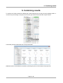
1
TmoleX
A Graphical User Interface to the
TURBOMOLE
Quantum Chemistry Program Package
User manual
COSMOlogic GmbH & Co. KG
Imbacher Weg 46
51379 Leverkusen, Germany
Phone +49-2171-363-668 Fax +49-2171-731-689
E-mail [email protected]
Web http://www.cosmologic.de
Version 4.1
June 2015
Page 2 / 92
Table of contents
1. Installation..................................................................................................................................................... 5
1.1. Windows............................................................................................................................................... 5
1.2. Linux..................................................................................................................................................... 6
1.3. Mac OS................................................................................................................................................. 7
1.4. Online Updates..................................................................................................................................... 8
2. A quick tour................................................................................................................................................... 9
2.1. Starting the program............................................................................................................................. 9
2.2. An illustrative example: Part 1............................................................................................................ 11
2.3. The tool bar......................................................................................................................................... 12
2.4. The sections....................................................................................................................................... 13
2.5. An illustrative example: Part 2............................................................................................................ 15
2.5.1 Geometry panel.............................................................................................................................. 15
2.5.2 Basis set panel............................................................................................................................... 16
2.5.3 Molecular start orbitals panel.......................................................................................................... 18
2.5.4 Level of theory: Select method....................................................................................................... 20
2.5.5 Start Job: Select kind of job and start it........................................................................................... 22
2.5.6 Results............................................................................................................................................ 24
2.6. Job Administration.............................................................................................................................. 25
3. The 3D visualization.................................................................................................................................... 27
3.1. The 3D builder.................................................................................................................................... 27
3.1.1 Navigation....................................................................................................................................... 28
3.1.2 Pre-stored structures...................................................................................................................... 29
3.2. Import structure................................................................................................................................... 30
3.3. Use SMILES code.............................................................................................................................. 31
3.4. The 2D Builder.................................................................................................................................... 32
3.5. Easy building: Paint tool...................................................................................................................... 33
3.6. Build complex molecules by merging fragments.................................................................................34
3.6.1 Building step by step 1.................................................................................................................... 39
3.6.2 Change bond length........................................................................................................................ 41
3.6.3 Change torsion............................................................................................................................... 42
3.7. Change bond angle............................................................................................................................ 43
3.7.1 Building step by step 2.................................................................................................................... 44
3.8. Pre-optimization.................................................................................................................................. 46
3.9. Labels and Measurements.................................................................................................................. 47
3.10. Moving, Rotating, Scaling................................................................................................................. 50
3.11. The gradient viewer.......................................................................................................................... 53
3.12. Surface plots..................................................................................................................................... 55
4. Properties................................................................................................................................................... 61
4.1. Vibrational frequencies....................................................................................................................... 61
4.2. IR spectrum........................................................................................................................................ 63
4.3. Nuclear magnetic shielding................................................................................................................. 64
4.4. UV/Vis and CD spectra (TD-DFT)....................................................................................................... 65
5. Constrained optimization and Scan jobs..................................................................................................... 66
5.1. Defining fixed internal coordinates...................................................................................................... 66
5.2. Use internal coordinates..................................................................................................................... 67
5.3. Start constrained optimization............................................................................................................. 68
5.4. Scan along an internal coordinate...................................................................................................... 69
5.5. Scan along several internal coordinates.............................................................................................70
Page 3 / 92
6. Job Templates............................................................................................................................................ 71
6.1. Define job templates........................................................................................................................... 71
6.2. Apply job templates............................................................................................................................ 72
6.3. Results of job templates...................................................................................................................... 74
7. Batch processing........................................................................................................................................ 75
7.1. Read in and use several molecules.................................................................................................... 75
Generate batch jobs from existing jobs...............................................................................................77
7.2. Apply templates for batch jobs............................................................................................................ 78
7.3. Run local or remote batch jobs........................................................................................................... 79
7.4. Visualize and export results of batch jobs........................................................................................... 83
8. Remote jobs................................................................................................................................................ 84
8.1. Security information............................................................................................................................ 84
8.2. Add new remote machine................................................................................................................... 85
8.3. Start a remote job............................................................................................................................... 87
8.4. Using a queuing-system on a remote cluster......................................................................................88
9. Combining results....................................................................................................................................... 92
Page 4 / 92
1.Installation
1. Installation
1.1. Windows
Prerequisites: Windows Vista, Windows 7, Windows 8 or Windows 10
The Windows version of TmoleX is distributed as a single executable file, called TmoleX_windows_4_1.exe.
To install TmoleX, simply double-click on TmoleX_windows_4_1.exe and follow the installation instructions.
After installation, TmoleX is available in your Windows Start Menu or as an icon on your desktop.
Please Note :
TURBOMOLE 7.0 for Windows is included in the TmoleX package. You will not have to install it additionally.
Some features of TURBOMOLE that are based on classical Unix scripts are not yet ported to Windows:
● Numerical second derivatives (script NumForce)
● automatic BSSE calculations (program jobbsse)
The
TURBOMOLE version for Windows(32bit) includes one generic type of serial 32-bit executable only,
without special optimization for a certain type of CPU. It runs on any processor that is compatible to the
Pentium 4 instruction set which supports SSE2.
The 32bit Windows version is not recommended for methods and jobs that require a lot of memory or CPU
time like coupled-cluster calculations. We recommend either the 64bit Windows version or the quantum
chemists work horse: Linux 64bit.
The
TURBOMOLE version for Windows(64bit) includes serial and parallel 64-bit executables. IBM's Platform
MPI Community Edition is included in the installer, parallel jobs should run out-of-the-box, but you have to
take care that the Windows firewall allows the processes to communicate with each other.
Page 5 / 92
1.Installation
1.2. Linux
Prerequisites: Linux distribution based on Kernel 2.6.x and newer.
The Linux version of TmoleX is distributed as a single file called TmoleX_linux_4_1.sh. Please make sure
that the file has execute permissions (chmod a+rx TmoleX_linux_4_1.sh) before starting it, then follow the
instructions on screen.
The full version of TURBOMOLE 7.0 is included in the TmoleX package.
Features that are not supported by TmoleX can be used by the command line version. After the installation
of TmoleX,
TURBOMOLE can be used from the command line as usual. Just set $TURBODIR to the
TURBOMOLE directory of the TmoleX installation, and extend the PATH to $TURBODIR/scripts and
$TURBODIR/bin/`sysname` (the binary directory).
Or, alternatively, a shell can be started by TmoleX with the correct settings by using the right-mouse menu in
the project list (see below).
Page 6 / 92
1.Installation
1.3. Mac OS
Prerequisites: Mac OS X 10.6 and newer
The Mac OS version of TmoleX is distributed as a single file called TmoleX_macos_4_1.dmg. To install
TmoleX, simply double-click on TmoleX_macos_4_1 and follow the installation instructions.
After
installation,
TmoleX
is
available
in
the
chosen
folder
(by
default
in
/Application/COSMOlogic/TmoleX14).
Features that are not supported by TmoleX can be used by the command line version. After the installation
of TmoleX,
TURBOMOLE can be used from the command line as usual. Just set $TURBODIR to the
TURBOMOLE directory of the TmoleX installation, and extend the PATH to $TURBODIR/scripts and
$TURBODIR/bin/`sysname` (the binary directory).
Page 7 / 92
1.Installation
1.4. Online Updates
TmoleX 4.1 includes an online update system and is able to automatically perform updates. This can be
initiated manually by checking for updates in the help menu. But TmoleX is also able to check for updates
itself. How often or if at all it should connect to COSMOlogic's update server can be chosen during the
installation of TmoleX:
Page 8 / 92
2. A quick tour
2. A quick tour
2.1. Starting the program
Starting TmoleX for the first time, you will get into the Welcome panel:
To start with TmoleX, create a new project by klicking on
.
Alternatively open an existing project (from former TmoleX versions) or watch the introductive online videos
first.
Page 9 / 92
2. A quick tour
All projects will require a new directory on your hard disk – where this directory shall be located and which
name it shall have is asked in the window that pops up:
The default directory is called TmoleXProject in your home folder. Just click on Select to accept the default or
generate a new directory and choose this one. You are now ready to perform your first Turbomole job:
Page 10 / 92
2. A quick tour
2.2. An illustrative example: Part 1
This section will guide you through the process of performing a DFT energy calculation and a ground state
geometry optimization of a molecule, for which input coordinates exist, e.g. benzene.
Option 1: Read in a coordinate containing file. The buttons
or
in the tool bar and the main window or the menu 'Import Coordinate File' in the pull-down menu 'File' will
open a file browser. Select the coordinate file and load the molecular structure of benzene into TmoleX
(first
change
to
your
home
directory
and
from
there
to
COSMOlogic/AppData/TmoleX15/fragments/rings/).
Option 2: click on 'Open 3D Molecular Builder' and double-click on the benzene entry on the right side
which is also located in the rings section.
Page 11 / 92
2. A quick tour
2.3. The tool bar
The tools in the tool bar act only on the job that you are currently working on, i.e. which is opened in the
project list.
Create new job within the current project.
Create new batch job within the current project.
Read or import coordinates (besides TURBOMOLE also many different formats).
Save/Export current coordinates in various formats.
Save current job to disk.
Open the directory of the current job in the default file browser of your OS.
Open molecular viewer. Can also be used to build new molecules.
TmoleX can run jobs on your local machine as well as on remote
systems. It also includes a simple queuing-system. By clicking on
either the local or the remote button a list of running jobs will
open.
The memory usage of TmoleX itself and the jobs
that are running on your local system is displayed here – click on
the TmoleX button (the yellow one in this example) to free unused
memory (starts Java garbage collector)
Page 12 / 92
2. A quick tour
2.4. The sections
TmoleX is structured as an interactive
TURBOMOLE input program, similar to the 'define' program, which
generates the input on the command line.
1. On the left you will find a list of open projects and jobs of each project,
2. on the top the general task menu (Geometry, Atomic Attributes, Molecular Attributes, etc.)
3. in the main frame the data assigned to the chosen task.
Page 13 / 92
2. A quick tour
The input is divided into four different sections:
The kind of job or property that shall be calculated can be set in the Start Job panel:
Results after a successful run can be viewed and further investigated in the Results panel:
You should follow the menu structure in the main frame from left to right. The traffic light
colors are indicating which steps have been accomplished and for which steps input is
needed.
Color code
Red: No valid data is available. User action required.
Yellow: Default settings available – unchecked by user so far.
Green: The data is correct or user did already visit this section.
Grey: Section is currently not available (like Results for a job which did not run yet)
Page 14 / 92
2. A quick tour
2.5. An illustrative example: Part 2
2.5.1
Geometry panel
After reading in the coordinates, you are in the
section. Here, you can choose the
symmetry, create internal coordinates, add atoms, or modify the structure.
Page 15 / 92
2. A quick tour
2.5.2
Basis set panel
The basis set is being defined in the
panel:
The basis set is def-SV(P) by default for all atoms. You have the possibility to select one basis for all atoms,
basis sets for given elements, or basis sets for individual selected atoms.
Hint:
If you are not familiar with the modern Karlsruhe/Ahlrichs type basis sets but with old
Pople type basis sets only:
6-31G*
is of similar quality than
def-SV(P),
6-31G**
--
def-SVP, and
6-311G**
--
def-TZVP.
Page 16 / 92
2. A quick tour
The drop-down selection 'Basis Set for all Atoms' contains just the Karlsruhe family of basis sets since those
are available throughout the periodic table.
For heavy elements a basis set which is optimized for two-component ECPs and two-component
calculations:
look at the automatically loaded ECPs
by clicking on
Selecting one of those will enable the relativistic 'Two component treatment' options in the Method section
later on.
NOTE: If you miss some basis sets which are present in the basis set library or if you have added own basis
sets to the basis set library, add them to the file basis_set_names.txt which can be found in the TmoleX
directory ( <Install-path>/COSMOlogic/TmoleX15/TmoleX/ ).
Page 17 / 92
2. A quick tour
2.5.3
For any
Molecular start orbitals panel
TURBOMOLE calculation an initial set of molecular orbitals is required. This is done with an extended
Hückel calculation in the
panel. If you do not (yet) have valid start orbitals, the button
will remain red.
If you click on 'Generate MOs', a message box will come up
Do not forget to set the molecular total charge before generating orbitals for IONS!!
Click 'Ok'. The generation takes only a (very) short time to compute and the initial molecular orbital are
displayed.
Page 18 / 92
2. A quick tour
The default for the multiplicity is automatic – TmoleX will generate molecular orbitals by doing an Extended
Hückel Guess and fills in the electrons according to the orbital energies. It will recognize closed and open
shell cases and switches to restricted (RHF) or unrestricted (UHF) settings.
Note that you have to generate new orbitals if you change the multiplicity. In this case, i.e. multiplicity not set
to automatic, will always result in unrestricted calculations!
In this panel you can also freeze core orbitals for correlated calculations or switch on Fermi smearing.
Switch from Table to Diagram to see the orbital occupation graphics. Use the left mouse button to set a
freezing point for frozen core approximation settings, and the right mouse button to zoom in (or click once to
zoom out).
Page 19 / 92
2. A quick tour
2.5.4
In the
Level of theory: Select method
panel you can choose the level of theory, activate COSMO, select auxiliary basis sets, and
advanced SCF settings can be changed.
The level of theory for your calculation can be set here. Currently nine different methods are available within
TmoleX:
•
•
•
•
•
•
•
Hartree-Fock
DFT
(with or without RI-J), RI-DFT is the default if you start a new session of TmoleX
DFT + Disp
DFT with empirical dispersion correction (with or without RI-J)
MP2
CC2
CCSD
CCSD(T)
Spin-scaled (SCS, SOS) MP2 or CC2 calculation can also be used as sub-options to the MP2 and CC2
level.
Page 20 / 92
2. A quick tour
Settings for SCF convergence and special COSMO selections (recommended only for expert users) can also
be found in the method section.
Energy and/or density convergence criteria can be entered in this panel. A density convergence criteria is
useful for properties and methods that need a very accurate density like post-Hatree-Fock methods or
TDDFT.
Note that the format of the parameters is different: The exponent has to be entered for the energy
convergence while the density convergence threshold is a total number like 1d-8 (use d instead of e like 1e8, because TURBOMOLE reads them in as double precision number). This difference is due to the fact that the
two corresponding
TURBOMOLE keywords, $scfconv and $denconv in the control file are have to be given
exactly like this – so TmoleX here tries to help to understand the default
TURBOMOLE input.
Changing the default DIIS damping settings might be needed for complicated electronic structures like
transition metal compounds. If the energy does not converge within many SCF iterations, the DIIS damping
factors should be increased. See the
TURBOMOLE manual for details about DIIS.
Page 21 / 92
2. A quick tour
2.5.5
In the
Start Job: Select kind of job and start it
panel, a single point energy calculation can be started.
'Run (local)' will start the calculation in the present directory.
'Save' writes the complete input to disk for further use on the command line or later usage if needed. Saving
the job to a directory will also add a script call start-job to the selected directory which can be used to start
the job on the command line.
'Run (network)' starts the calculation on a remote Linux/Unix computer, see chapter 8.
Page 22 / 92
2. A quick tour
Click through the Job type options to see what kind of jobs are supported by TmoleX.
Depending on the job type, different options for the chosen job are displayed in the Options section. The
Method section briefly summarizes the settings done in the four menus before (method, symmetry, basis set,
etc.).
Finally, the 'Use resources' part can be used to set (maximum) amount of memory (RAM) and disk space for
the calculation. If and how important those settings are depends on the method and job type. For ground
state single-point energies and geometry optimizations at Hartree-Fock or DFT level, neither more memory
nor more disk space will speed up the calculation significantly. For vibrational frequencies (IR and Raman
spectra), post-Hartree-Fock methods or excited state calculations, more memory can improve efficiency a
lot.
Please note that the given memory value is not the total amount of RAM the program will use, just the parts
that can be adjusted. Hence, do not enter more than roughly 80% of your total memory here to avoid huge
performance problems!
Page 23 / 92
2. A quick tour
2.5.6
Results
Whenever a calculation is finished, you can find a summary in 'Results'. The output files and a viewer (see.
next chapter) can be opened from here.
Important:
•
•
Check the Status of the molecular orbitals and the status of the geometry optimization!
In case that the orbitals (MOs) are not converged, restart the job – perhaps more SCF iterations or
higher DIIS damping is required (see Method section)
•
•
If the geometry is not converged, restart the optimization allowing more geometry cycles.
Also make sure that the HOMO-LUMO gap is positive. Otherwise you have a hole in the occupation
(which might be what you want, but usually this should not be the case), and you did not get the
proper ground state of the electronic structure.
Page 24 / 92
2. A quick tour
2.6. Job Administration
job_GEO
indicates a
geometry
optimization
choose Project
in ProjectList to
get a list of all
jobs
Job-Type gives
a very short
description of
the most
important
settings
Start/Stop for
timings and the
status if job is
still running
While the job is running and if you select the project itself in the project list on the left, the lower part of the
TmoleX window will show the current status of the selected job (there is just one job on the example above).
Click on the name of the Project in the ProjectList and use the right mouse menu in the 'Jobs' section to
close (remove just from the list, let all files on disk), stop (stop running jobs, let files on disk), delete (delete
job from the list and delete the files from disk) jobs. 'View Job directory' will open the default file browser on
your system with the directory where the selected job is running or was running. 'View run status' can be
chosen for running jobs.
The progress and status of all calculation belonging to your project, which are currently running or ran
Page 25 / 92
2. A quick tour
before, can be accessed via the “Job-Administration” by clicking on the project name itself instead of a job
within the project. After starting a first job, you can instantly set up and even launch a new one. For
performance considerations you will however prefer running only one job at a time in most cases.
Note: TmoleX does not yet cover all possible kinds of calculations and input options that
TURBOMOLE
offers. If you need additional options but want to use TmoleX, you can manually edit the control file. Please
refer to the TURBOMOLE manual for further information.
Internal simple queuing system
Set the number of cores of your machine in the Extras → Settings menu. Then, TmoleX will take care of the
number of jobs you are starting:
The green section is related to the memory usage. First by TmoleX itself (click on the button to start Java's
garbage collector to give free unused memory) and then by the jobs which are running (estimated from your
memory settings when starting those jobs).
The grey section shows the number of local and remote jobs. Note that only jobs from open projects are
shown – closing a project with running jobs will is not recommended as TmoleX will loose the connection and
might not be able to correctly reopen them!
Whenever the number of running local jobs is exceeded, TmoleX will start the next job only after another one
has finished. Several jobs can be started that way without blocking your system. The jobs that are scheduled
for running are shown with an own icon in the job list.
Page 26 / 92
3.The 3D visualization
3. The 3D visualization
3.1. The 3D builder
To open the molecular builder click on either the button in the tool bar or the button in the Geometry panel of
TmoleX:
The molecule builder can be used most conveniently by starting from fragments and modifying these.
Double-click on a fragment to import it in the builder.
Page 27 / 92
3.The 3D visualization
3.1.1
Navigation
Left mouse button or
or q on the keyboard: Select
Right mouse button or
:
Rotate view
Middle mouse button or
:
Move
Scroll wheel or
:
Zoom
Page 28 / 92
3.The 3D visualization
3.1.2
Pre-stored structures
There are different ways to add molecules and fragments which build up a structure.
Double-click or drag-and-drop molecules from the Molecules section on the right to the window:
The molecules in the right part of the window are by default taken from the fragments directory of the TmoleX
installation. This can be changed to a user-defined directory in the Tools → Visual settings menu:
The files are stored in standard sdf format, and a second file with the same name but .sdf.fr ending is being
generated.
The fr file contains two lines:
•
the first one represents the number of the atom which will be replaced when using the 'Substitute
with...' option in the right mouse panel (see below)
•
the second line can contain the name of the fragment the way it will be displayed in the 'Molecules'
section of the builder.
Page 29 / 92
3.The 3D visualization
The replacement atom can be chosen with the right-mouse button menu:
The File → 'Save to Fragment directory...' menu can be used to store the structure that is visualized
in the 3D window to the users data base. The atom that is selected when saving is the one that will
be replaced.
3.2. Import structure
Instead of building a molecule from scratch, an existing molecule in different formats (sdf, ml2, xyz, cosmo,
…) can be imported using the File/Open menu entry within the visualizer.
This structure can then be used for modification or being saved in the user data base as described above.
Page 30 / 92
3.The 3D visualization
3.3. Use SMILES code
Most organic compounds can be described with the SMILES notation
(see https://en.wikipedia.org/wiki/Simplified_molecular-input_line-entry_system)
and there are several web sites which provide SMILES code for a large number of structures like
ChemSpider (http://www.chemspider.com/).
If you have a SMILES code, there are two ways to add it to the 3D builder:
1. directly in TmoleX in the geometry part of the input generation, just add the SMILES code to the field
shown below and click on
:
Enter or paste your SMILES here
2. or in the Builder if the Molecules section is selected, add it to the SMILES field and click on the
button:
… or enter it here
The difference is that clicking on the
in TmoleX will replace whatever you already had as
structure in the Builder, while adding SMILES to the Builder itself will act as adding one of the fragments or
structures of the fragment library.
The SMILES to 3D conversion is done using RDKit (http://www.rdkit.org/).
Page 31 / 92
3.The 3D visualization
3.4. The 2D Builder
If you start the 2D builder, click on
to open a new window of JChemPaint
Draw your structure in JChemPaint and click on 'Get SMILES' or 'Get SMILES and close' to copy and paste
the resulting SMILES of your painting into TmoleX and the 3D builder (if open).
Detailed information about JChemPaint can be found on https://jchempaint.github.io/
3. Add to 3D Builder
1. Draw
2. Get SMILES
Page 32 / 92
3.The 3D visualization
3.5. Easy building: Paint tool
A quite handy way to build is the paint tool
which can be chosen by clicking on the
button or hitting the D key on the keyboard.
In the paint modus, select an atom or a molecule from the Molecules/Atoms section in the builder:
This will change your cursor to the element symbol:
to add a C or
to add a nitro
group, resp.
Click on the background to add the atom or molecule or click on an existing atom to replace it with the
selected atom/fragment.
Click on the
hydrogen
Page 33 / 92
3.The 3D visualization
3.6. Build complex molecules by merging fragments
a) Load two molecules, select one atom from each of two different fragments:
b). Use the right mouse button and select the Merge option. TmoleX will join the two fragments and rearrange the resulting structure such that the overlap of the atoms is minimal:
Page 34 / 92
3.The 3D visualization
To merge two fragments which are not just connected by one bond, a
more powerful option is to merge overlapping atoms.
a) read in two benzene
b) move one fragment close to the second one. This can be done in two ways:
i) select one of the two benzene by double-clicking on one atom and then select the translate tool
(or hit w on the keyboard)
Hold left mouse button and move the fragments such that they overlap (switch to another direction
and/or use the 'along view' button to move in the direction of the monitor system of coordinates).
Page 35 / 92
3.The 3D visualization
ii)create a bond between two atoms, select it and change its length to zero
iii)
and even easier: Select two bonds of the two benzene rings and select 'Merge bonds'
The moved fragment should look like this:
The zero-bond length method leads to:
Page 36 / 92
3.The 3D visualization
Double-click on the background (or hit the Esc key or use the left mouse button) to get to selection mode.
Draw a box around the overlapping part and select 'Merge overlapping atoms' from the right-mouse button
menu:
All atoms which have a (little bit) of overlap will be joined in a way that the lighter atoms is being deleted.
Page 37 / 92
3.The 3D visualization
The trick to set a bond length to zero works only in cases where the selected bond is not part of a ring!
Page 38 / 92
3.The 3D visualization
3.6.1
Building step by step 1
Change to selection mode (q or ESC key or arrow button on the left side) if you are not already in this mode.
Select an atom:
On the right side the properties of the selected item (atom, bond, measure, etc.) are shown.
For objects which are hard to select with the mouse, the Objects chooser can help since it contains all
displayed objects, including measurements and constraints.
Most entries can be changed in the fields.
Page 39 / 92
3.The 3D visualization
Change the Element from H to C and also the Hybridisation to sp3(tetrahedral):
Next, click on
to add missing hydrogens to the selected atom according to the given hybridisation.
Page 40 / 92
3.The 3D visualization
3.6.2
Change bond length
Now the bond length to the newly created methyl group is set to a default single-bonded C-C lenght, but can
be changed by selecting the bond. Either enter a new value or let TmoleX guess the length according to vdW
radii:
The length and also many other things can be done by using the context menu of the right mouse button:
Hint: If you want to change a bond length (or an angle or torsion) and there are no bonds to select, simply
add a new bond between two selected atoms using the right mouse menu.
Page 41 / 92
3.The 3D visualization
3.6.3
Change torsion
To change the dihedral angle, click on the middle bond or select three bonds (holding shift key will add
selections) which define the angle and then either use the button on the left that will show up or again the
right mouse menu:
The torsion around which the molecule will be rotated is being shown. Use the left mouse button to change
the angle – moving to right or up will increase the value, moving the mouse to the left or down will decrease
the angle. The value of the angle can be entered directly on the right side, and one can also choose if the
smaller or the bigger fragment is being moved.
Page 42 / 92
3.The 3D visualization
3.7. Change bond angle
To change a bond angle, select two adjacent bonds (shift-click for the second one) and either click on the
button on the left side or use the right mouse button to change the value:
The properties of the angle are shown and can either be changed by clicking on the left mouse button and
dragging the mouse or by editing the field:
Like for torsional angles, the small and big fragment option decides which part of the molecule is being
moved.
Page 43 / 92
3.The 3D visualization
3.7.1
Building step by step 2
Instead of changing an atom to a different element, to change hybridisation and use the saturate option, an
atom can also be replaced by a pre-stored fragment.
Select an atom, use the right mouse button and click on 'Substitute with'.
Note: The fragments that are shown are the molecules of the user data base (or the default pre-stored
molecules after installation as shown here). When choosing Attach, the connecting atom – which was
marked as such when saving the structure to your fragment data base – will directly be substituted.
The builder will automatically switch to the
dihedral mode. Use the left mouse button
to rotate around the new bond. To get
back to the selection mode, double-click
on the background, hit the Esc key or use
the
button.
Page 44 / 92
3.The 3D visualization
Alternatively any other atom can be used as connecting atom:
Choosing 'Attach with custom atom' will open the structure of the fragment in an own window.
Just click with the left mouse button on the atom (one of the hydrogens in this case) to select the
connecting atom.
Page 45 / 92
3.The 3D visualization
3.8. Pre-optimization
There are three options to pre-optimize a guess structure:
•
Unselect all objects by clicking on the background
Use the right mouse button and select:
A simple rearrangement which minimizes the overlap of the van-der-Waals radii of all atoms
•
UFF – a universal force field as implemented in TURBOMOLE can be used by clicking on the FF button:
•
The recommended way is to use MOPAC7, which is included in the default installation of TmoleX.
The MOPAC7 button will open a new window with several options.
AM1, PM3, MNDO, MNDO/3 are the available methods (they all are parametrized for a certain
number of elements). AM1/COSMO is the default setting for COSMOtherm input files at BP-SVP
level (first do a geometry optimization at this level and then a single-point DFT calculation with
COSMO and SVP basis set). Unrestricted calculations can be done with UHF, guess structures for
transition states can also be searched. A molecular charge has to be entered to calculate ions.
Page 46 / 92
3.The 3D visualization
3.9. Labels and Measurements
Labels for atoms and bonds as well as measures of lengths and angles can be switched on or off for the
complete structure or individually for each object.
•
Display labels for all atoms or bonds
In the 3D viewer select Tools → Visual settings and switch to the Labels section:
For atoms the atom number, the element symbol, the charge and additional text (which can be
entered by the user with the right mouse button menu within the viewer window) can be displayed.
Depending on the background colour and the colour of bonds and atoms the labels can be hard to
read. The background settings here refer to the background of the text field only.
Page 47 / 92
3.The 3D visualization
•
To display labels of one or several atoms/bonds only, use the right mouse menu:
Own text can be entered in the second item of the right mouse menu. To add or remove labels for
several atoms or bonds, just select several items and then use the right mouse button for the
selection.
•
Measures can be added with the right mouse menu, what is measured depends on what you have
selected:
◦ select two atoms: measure distance
Page 48 / 92
3.The 3D visualization
◦ select two bonds: measure angle
◦ select three bonds: measure torsion...
Measures can be selected and deleted with the Measures pull down list:
Page 49 / 92
3.The 3D visualization
3.10. Moving, Rotating, Scaling
It is often helpful to move or rotate parts of the molecule to a new position. This can be done within TmoleX
with several powerful possibilities, but the usage is not self-explaining. So here are the options:
•
Select several atoms,
hold shift key and select the atom around which the rotation shall be done. The last atom that is
selected will be by default the centre of the rotation! Use the right mouse menu or the button
or the key 'e' to switch to rotation mode.
Rotation of the selected atoms can be done using x,y,z axis as rotation axis. In addition to that, the
yellow circle indicates the rotation around the axis that is perpendicular to your screen – at the
moment you activate the rotation mode. Use the right mouse button to rotate the view, the middle
Page 50 / 92
3.The 3D visualization
mouse button to move the camera and the scroll wheel for zoom. Those mouse movements will not
change the coordinates, just the view.
To rotate around x,y, z, or the initial view direction, use the left mouse button and drag the mouse.
Use the coloured buttons on the right side of the window to switch the rotation axis, or click directly
on the coloured circles.
The 'around view' button will reset the yellow 'view' rotation axis to your current viewing direction.
Note that rotating the view with the right mouse button does not change the rotation axis!
The 'Pivot at COM' changes the centre of the rotation to the centre of mass of the selected atoms.
Rotation angles can be entered (in degrees) to the corresponding X,Z,Y, View fields. The center of
rotation, i.e. the pivot, can also be entered manually if needed.
Note that the selected atoms which will be rotated do not have to be connected.
•
Moving atoms or fragments is very similar to the rotation procedure described above. Select the
atoms that shall be moved and use the right mouse menu (Translate), or the button
, or press
the key 'w'.
Hints:
◦ Double-click on an atom to select the whole fragment (all atoms that are connected by bonds).
◦ There is an option 'Select bond partners' in the right mouse menu which extends the selection
around each already selected atom to its next (bonded) neighbours.
Page 51 / 92
3.The 3D visualization
Again, change the direction of movement either by clicking on the coloured buttons on the right side,
or by clicking on the coloured arrows.
Note:
◦ Holding the left mouse button and moving the mouse to the right or up will move along the
positive direction (plus x,y,z values), and moving the mouse down or to the left will decrease the
coordinates – no matter from which direction you are looking at the structure! This can
sometimes lead to the fact that moving, for example, the mouse to the left will move the fragment
to the right (because you are looking at the structure from 'behind').
◦ Again, in addition to the absolute directions x,y,z, you can move the selected atoms along the
direction that corresponds to the 2D coordinates of your screen: Right/Left and Up/Down. Click
on 'along view' to reset the Right and Up direction to your current view on the structure.
•
Finally, the scale tool
(key 'r') scales or resizes relative distances between atoms. Add a
benzene ring, select it, and use this tool to see what it does.
Page 52 / 92
3.The 3D visualization
3.11. The gradient viewer
Once you have completed a geometry optimization, you can open the gradient viewer from the results panel.
Page 53 / 92
3.The 3D visualization
The total energies for the optimization steps can by viewed here.
The different geometry can also be viewed as a movie by using the play buttons or moving the slider. The
smaller < and > go stepwise back and forth. It is also possible to click on one of the circle in the graphics on
the right which plots the total energy vs the geometry cycle.
The 'Calculate bonds' check can be set to re-check the bonds with respect to the atom distances in each
step.
Page 54 / 92
3.The 3D visualization
3.12. Surface plots
Once you have converged molecular orbitals,
TURBOMOLE offers the possibility to write different properties on
a grid for a visual post-processing. This is reproduced in TmoleX interactively starting from 'Orbital/Density
Plot'.
Page 55 / 92
3.The 3D visualization
The new window which opens allows you to generate 3D data for visualization as well as to start the 3D
viewer with previously or newly generated data:
The upper section is the list of molecular orbitals, the lower section is for electrostatic and density derived
properties.
For each of the properties there are two options: 'quick' and a 'high-res'. The first one is to generate the data
on a coarse grid to keep the time for generating the 3D files low. This is useful to quickly check the shape
and position of orbitals, densities, etc. The second option generates the data on a finer grid, generating
smoother surfaces, but can require significantly more CPU time to generate the data. This is recommended
for graphics aimed for publication.
Page 56 / 92
3.The 3D visualization
There are three possibilities to generate 3D data:
1. directly click on one of the buttons
and TmoleX will directly start to generate the data.
2. set checks in the first column for each orbital and property you want to visualize and then click on
.
3. as usual, a right mouse menu is available. Simply select one or several lines in the tables and click
on the right mouse button.
Page 57 / 92
3.The 3D visualization
If you choose several options like orbitals, densities, electrostatic potential, etc., each property will have its
own progress bar. All properties which require solving integrals like electrostatic properties, densities and
their derivatives are quite expensive. Especially for larger molecules, generating 3D plot files can take
(much) longer than the single-point calculation or a geometry optimization!
When the calculation is finished, the orbitals or properties can be selected for visualization. Several
properties can be displayed in the same window. Check the memory usage of TmoleX from time to time
when using this option!
Just click directly on the buttons which have now a green check to show that 3D data is already available for
visualization:
Alternatively, use the right mouse button or the selection column and the 'View selected' button.
Page 58 / 92
3.The 3D visualization
There are a lot of options and possibilities when visualizing 3D surfaces. The most important things are:
•
while it can be annoying that the full 3D grid is being calculated, which can be very time consuming,
TmoleX can now use this data to generate the 2D surface for a given iso-value on-the-fly.
Use the slider or the field for the iso-value to change the threshold.
•
The 'Display' options are:
◦ isosurface – use one iso-value to plot the surface at this value
◦ cloud – plot each point of the 3D grid which is within the Min and Max value. The colours of the
points depend on the Min-Max range.
◦ Isoplot – plot a plane (or an arbitrary surface which can be given as implicit equation like
x^2+y^2+z^2-4. Avoid blanks and let the mouse pointer rest over the field to get some help)
coloured with the value of the chosen property. Colour depends on the Min-Max range. If you
see nothing, not enough, or not enough colours, change Min and/or Max value.
◦ Isoplot again – click 'on isosurface' and a file chooser will open. Click on e.g. td.plt (total density)
and set an iso-value below. This will result in a 2D surface which represents the iso-value of the
density and the colour on the surface is given by the value of the chosen property at that points.
Typical example: open electrostatic potential, use the isoplot option, choose td.plt for the total
density and set an iso-value. This will give a typical picture of a electrostatic potential on an
density-isosurface.
◦ Isosurface +/- – plots two iso-densities: one at the positive value and one at the negative value.
A typical molecular orbital picture.
Page 59 / 92
3.The 3D visualization
Vector plots
Vector fields can be visualized too, the best way to get an idea of the field depends on the property. Most
options are similar to those described above.
Page 60 / 92
4.Properties
4. Properties
4.1. Vibrational frequencies
If you have an optimized geometry, you might want to follow it up by a frequency calculation, either in order
to check, if you are in minimum, or because you are interested in the IR spectrum.
Choose 'IR & vibrational frequencies' in the 'Start Job' panel and click on Run.
In addition to analytic 2nd derivatives, TURBOMOLE is also able to perform 2nd numerical derivatives for all
properties which have an analytic gradient implemented. For post-Hartree-Fock calculations or if COSMO is
switched on, the numerical option is chosen by default.
NOTE: 2nd numerical derivatives can not be performed with the Windows version of TmoleX. Please submit
such jobs to (remote) Linux systems.
Page 61 / 92
4.Properties
To visualize the vibrational frequencies and/or to distort the structure along a vibrational mode, start the 3D
Viewer by clicking on the 'Vibrations' button.
Select a specific mode and click 'play'.
Select one or several modes first. Use the play buttons and/or the slider to see the vibration.
Page 62 / 92
4.Properties
4.2. IR spectrum
Use the
to open the IR spectrum:
Standard deviation for the broadening Gaussians or Lorentzains, a frequency shift, number of sampling
points, etc. can be entered. The tables with the original data (line spectrum) and calculated data (points that
define the broadened lines) can be used to copy and paste the data to a spread sheet or a statistics
program.
Page 63 / 92
4.Properties
4.3. Nuclear magnetic shielding
For the calculation of nuclear shieldings choose this job type and simply run it.
In the 'Results' panel you can see the shielding constants in a text window.
Copy and paste the values to a spread sheet for further usage. Note that to get the NMR shifts, you have to
do a calculation also on the reference molecule (like TMS for carbon) with the same method and basis set.
The NMR shieldings can also be displayed as labels in the viewer, click on 'NMR Shieldings' to open this
view.
Page 64 / 92
4.Properties
4.4. UV/Vis and CD spectra (TD-DFT)
A TD-DFT calculation is set up like a normal DFT calculation. Then choose 'Excited States' in the job
selection
This opens a new option section for the job. Select singlet or triplet, either full (RPA) TDDFT or using the
Tamm-Dancoff (TDA) approximation, the number of excitations, and run it.
The spectra can be opened with the CD or UV/Vis Spectrum button.
Page 65 / 92
5. Constrained optimization and Scan jobs
5. Constrained optimization and Scan jobs
5.1. Defining fixed internal coordinates
TmoleX allows to define internal coordinates. Bonds, bond angles and torsions can be fixed within the
builder.
To define a constraint, select one, two or three bonds:
•
select one bond, click on the right mouse and choose Scan/freeze length:
On the right the options for freezing a bond length are show:
To delete constraints, select here and
delete.
To scan along the coordinate, activate the
check box and set minimum, maximum
and
the step width (not the number of steps!)
•
Select two adjacent bonds, click on the right mouse button and use the Scan/freeze bond angle
Page 66 / 92
5.1.Defining fixed internal coordinates
option:
Again, on the right side you will get the same options for scan jobs as shown above.
•
Select one or three bonds to freeze a torsion. If you just select one, TmoleX will take just one of the
possible torsional angles. If you use the 'Change torsion' or the corresponding button on the left side
of the window, the value of the internal coordinate is shown and can be changed as usual with
dragging the mouse while keeping the left mouse button pressed.
Page 67 / 92
5.2.Use internal coordinates
5.2. Use internal coordinates
TmoleX will automatically generate a list of internal redundant coordinates if you accept that when being
asked for. If you use constraints or scan jobs, internal redundant coordinate usage must be activated when
starting a geometry optimization!
Be careful with linear combinations (several lines of definitions for one internal coordinate) – while they can
be fixed, this is usually not what one really wants!
There is a possibility to visualize the set of internal redundant from within the Geometry panel.
5.3. Start constrained optimization
A constrained search is automatically done if a usual geometry optimization job is started while having
internal (or Cartesian) coordinates fixed. TmoleX will show a message in the panel whenever such jobs are
started:
If you have frozen bonds, angles or torsions, make sure to use internal redundant coordinates, otherwise
your settings will be ignored! As long as you have constraints defined it is not possible to run an optimization
without internal coordinates.
Constrains are always applied in this section, no matter if ground or excited states calculations are done,
minimum search (geometry optimization), potential energy scans, or transition state searches are started.
Page 68 / 92
5.2.Use internal coordinates
5.4. Scan along an internal coordinate
The potential energy scan (PES) method can be applied if internal coordinates are defined, and at least one
of them is defined as fixed. Scan will run a couple of geometry optimizations for a range of values of an
internal coordinate.
Note that all fixed internal coordinates will be kept fixed, not just the one that you have defined to be
scanned along! For a one-dimensional scan job, only one internal coordinate should be defined as fixed.
The list of fixed internal coordinates is shown in the PES scan Options section. To define a new fixed internal
coordinates, use the
button. This is not needed if you did that in the builder
already.
The different options how the start geometries are generated are described in the panel itself. Unrelaxed
scans and relaxed scans are possible (single-point or geometry optimization calculations will be done).
We recommend to use the 'Use current structure for all' option, because if one of the steps fail, the remaining
jobs will have problems too otherwise.
Page 69 / 92
5.2.Use internal coordinates
The job can then be started as usual, also as a remote calculation. A typical result is shown here:
The final optimized structures are stored for each of the scan points in a multi-coord file – similar to the
gradient view. This can be viewed like a movie with the button
.
5.5. Scan along several internal coordinates
The number of internal coordinates which can be used for scans is only limited by technical issues. If, for
example, the number of constraints is – relative to the number of degrees of freedom – very high, TmoleX
might not be able to generate all intermediate structures of all combinations due to steric reasons.
It is also possible to combine constraints (like fixing an angle to a certain value) with scans. If the number of
internal scan-coordinates is larger than one, TmoleX will not show a graph of the result but just the table with
the values of each internal coordinate and the total energy in the last column. This table can be exported to a
spread sheet program or other data analysis tools.
Page 70 / 92
6.Job Templates
6. Job Templates
6.1. Define job templates
TmoleX gives you the possibility to save the most important settings of your jobs like basis set, method or job
type to a template. This helps to reduce the time needed for an input preparation if the same kind of job has
to be performed for a set of molecules.
To read, modify or create a job template, choose 'Templates' from the TmoleX menu:
Read in existing template to modify or apply.
Create new job template.
Click on
to add a job to the workflow.
MOPAC pre-optimization only possible in
first job. Make sure not to switch on the
symmetry check in the following Turbomole
jobs.
The settings here are the same as in the
different TmoleX panels.
Save the template or apply it without saving.
The settings are quite self-explaining.
But at this point, TmoleX does not check for consistency of different settings. So please do first a usual job,
run it, and check if the combinations are possible.
Defining multiple jobs in one job template will tell TmoleX to run them one after the other, using the
coordinates of the preceding step.
job 1
Use final coordinates
of job 1
job 2
Use final coordinates
of job 2
Page 71 / 92
job 3
Use final coordinates
of job 3
….
6.Job Templates
A typical work flow would be:
RI-DFT geometry optimization with small basis set → frequency analysis → geometry optimization with
larger basis set → CD + UV/Vis spectra at DFT level→ single point energy calculation with post-HartreeFock method.
The template will have to be named when saving and can be found in the pull-down menu afterwards.
6.2. Apply job templates
To use a template, just choose a saved template from either the template tool bar:
or from the menu 'Templates'. TmoleX will alter the settings accordingly, generate start orbitals, and brings
you directly to the start-job panel.
The molecular charge can be either those of the template (if the Charge pull-down menu is let empty) or
whatever the user chooses in the tool bar.
Generate a new job, read in or build a molecule. Then select a template (set the charge or use the default)
and click on
. TmoleX will prepare the input and jump to the start job panel:
The job can either be started on the local system or submitted to a remote machine using the Run(network)
button.
While the job is running, the icons in the job tree will change. The job status during the run can also be
displayed and visualized:
Here the first job, a geometry optimization, is running. The status of this job is therefore printed as Energy vs.
the geometry cycle.
Page 72 / 92
6.Job Templates
Page 73 / 92
6.Job Templates
6.3. Results of job templates
Multi-template jobs will create sub-directories for each individual job. Selecting an individual job will present
the results of this step as for a usual non-template job. Selecting the template itself in the job tree will give a
summary as table:
Here an example of ethanol, the job template was GEO+OPT from the predefined list of job templates.
Page 74 / 92
7.Batch processing
7. Batch processing
The job templates described in the previous chapter can easily be applied to any kind of structure, the user
does not have to take care of anything else but to read in the coordinates or build a molecule, set the charge
or accept the defaults, apply the template and start the job.
To open a new batch job, just use the File → New Batch Job entry in the menu or click on the
the tool bar. TmoleX will generate a new job, the geometry menu of this job is shown:
button in
7.1. Read in and use several molecules
Batch jobs apply predefined job templates to a list of molecules. The molecules have to be read in from file
by using the
button. This opens a file browser which also allows to read in file formats which
contain multiple structures like sdf. Multiple selections within the file browser are of course also possible.
Page 75 / 92
7.Batch processing
The charge may or may not be imported correctly, so check and eventually change the charges in the
table!
The multiplicity can also be changed, but it is recommended not to do that since TmoleX will use the
TURBOMOLE default it determines from a Hückel calculation.
Ions are shown in different background colours, a quick look on the table should to sufficient to identify nonneutral compounds.
Double-click on a graphical representation of the molecules to open the builder.
Page 76 / 92
7.Batch processing
Generate batch jobs from existing jobs
Another possibility to generate a new batch job and to read in structures is to select a list of finished jobs in
your project and job tree and click on the right mouse button.
Page 77 / 92
7.Batch processing
7.2. Apply templates for batch jobs
Once you have a complete list of molecules to perform calculations on, select a job template from the tool
bar.
Important: The charge field can either have numeric entries which will assign the given charge to all
molecules, or it can be empty – in this case the charges that are displayed in the table will be
used. The default, which applies when no charge is imported from the coordinate files, is zero.
All settings for basis set, method, job type, etc. can not be changed in batch jobs since they are defined in
the job template. In this example the charge field is empty, so TmoleX will use the charges printed in the
table. Otherwise they are overwritten.
Before starting a batch job, you have to click on
to assign all settings of the template to
your individual jobs. Possible errors or problems can thus be detected before the whole batch is started or
sent to a remote system. This process can take some time, depending on the number and size of the
molecules as well as the number of steps defined in your template.
After applying the job template, a short overview is printed in the Start Job section:
Page 78 / 92
7.Batch processing
7.3. Run local or remote batch jobs
After a job template has been applied and TmoleX has finished to generate the input files of all steps and for
all molecules in the list, the complete set of calculations can be simply started as you would start a usual job.
So either use the
button to use the system TmoleX is running on, or the
button to submit everything to a remote system.
While the job is running the icons in the job list on the left side of your TmoleX window will show their current
status.
On remote systems the resulting files will only be copied back after all steps have finished to avoid too much
traffic on the network. TmoleX, however, checks from time to time which job is currently running and whether
or not the whole batch is complete. For single jobs which are finished but not yet transferred back to your
local desktop machine, the icon switches to
.
Page 79 / 92
7.Batch processing
Using many cores or CPUs on your local system
As you can see in the screen shot printed above, several different jobs can run at the same time when a
batch job is being used. To be able to use several CPUs on your system, you have to tell TmoleX how many
of them you allow the program to use on your local machine.
To do that, just select the Extra → Settings entry in the menu and you will get a new window:
Set the number of available processes here, but it is recommended not to use all available cores to let at
least one of them free for being utilized by TmoleX and your operating system.
When starting the job, just set the number of CPUs in the Start job panel directly:
Page 80 / 92
7.Batch processing
Using many cores or CPUs remote systems
Similar to the local system settings, you can also set the number of CPUs on remote systems using the Extra
menu:
this will open:
There is the entry:
•
Use CPU – the total number of CPUs TmoleX is allowed to run on that system (for all jobs).
The default is -1 which is equivalent to unlimited.
To see how many jobs are already running on the remote system, use the right mouse button menu and click
on 'Check workload'. This will call 'top' on the remote system and show the results:
Page 81 / 92
7.Batch processing
In the first line, the load, i.e. the number of running (time consuming) processes is shown. If you did set the
number of total CPUs on the remote system as described on the last page, it is also shown here as 'available
CPUs'.
The three entires are:
•
•
•
current
–
number of CPUs in use right now
~ 5 min. ago
–
number of CPUs in use approximately 5 minutes ago
~15 min. ago
–
number of CPUs in use approximately 15 minutes ago
This gives quite a helpful hint how occupied the system already is and whether or not some new jobs have
been started recently or how many old jobs stopped in the last 15 minutes.
If you activate the 'Show expert information' check box, you will see the detailed output of 'top' – which users
run which jobs on the machine, how much CPU time and how much memory they use. In the example given
here, only the user tmolex is running jobs (entries with significant %CPU values).
Page 82 / 92
7.Batch processing
7.4. Visualize and export results of batch jobs
The results of finished batch jobs are given as tables in the Results section. Each sub-job has an own tab in
the table.
The resulting table can be saved as spread sheet. The Export Files button allows to save COSMO, energy or
coordinates files of different format:
COSMO and energy files are usually only needed for the COSMOtherm program. TmoleX will save all files of
the given type to the chosen directory.
Page 83 / 92
8.Remote jobs
8. Remote jobs
TmoleX as well as the client version of TmoleX which is freely available from COSMOlogic web site is able to
start jobs on remote Linux/Unix machines using a secure shell.
8.1. Security information
To determine if you do want to use this feature and worry about security, here is a short outline of the
procedure used by TmoleX to access to remote systems.
•
ssh and scp are used to start jobs and to copy the files from one system to another.
We use a locally modified version of PuTTY (http://www.chiark.greenend.org.uk/~sgtatham/putty/)
PuTTY is copyright 1997-2009 Simon Tatham.
Portions copyright Robert de Bath, Joris van Rantwijk, Delian Delchev, Andreas Schultz, Jeroen
Massar, Wez Furlong, Nicolas Barry, Justin Bradford, Ben Harris, Malcolm Smith, Ahmad
Khalifa, Markus Kuhn, Colin Watson, and CORE SDI S.A.
Permission is hereby granted, free of charge, to any person obtaining a copy of this software
and associated documentation files (the "Software"), to deal in the Software without restriction,
including without limitation the rights to use, copy, modify, merge, publish, distribute,
sublicense, and/or sell copies of the Software, and to permit persons to whom the Software is
furnished to do so, subject to the following conditions:
The above copyright notice and this permission notice shall be included in all copies or
substantial portions of the Software.
THE SOFTWARE IS PROVIDED "AS IS", WITHOUT WARRANTY OF ANY KIND, EXPRESS
OR IMPLIED, INCLUDING BUT NOT LIMITED TO THE WARRANTIES OF
MERCHANTABILITY, FITNESS FOR A PARTICULAR PURPOSE AND NONINFRINGEMENT.
IN NO EVENT SHALL SIMON TATHAM BE LIABLE FOR ANY CLAIM, DAMAGES OR OTHER
LIABILITY, WHETHER IN AN ACTION OF CONTRACT, TORT OR OTHERWISE, ARISING
FROM, OUT OF OR IN CONNECTION WITH THE SOFTWARE OR THE USE OR OTHER
DEALINGS IN THE SOFTWARE.
•
PuTTY uses its own repository for public ssh keys, so ssh connections that do not require a
password on your local machine at the command line might not work if OpenSSH or any other ssh
program is used. Run ssh from the TmoleX directory to check that manually.
•
jobs can be killed while they run on a remote system. For that purpose, a kill-job script is being
stored in the directory where the job is running. This script does kill all processes that are running in
the directory the script itself is located – but this will only work on systems where a /proc directory is
present (usually all Linux systems and most Unix systems either).
•
Passwords entered in the password field will not be saved to disk. Hence, they have to be entered
each time TmoleX has been started, but kept in memory as long as TmoleX runs.
Page 84 / 92
8.Remote jobs
8.2. Add new remote machine
When starting a remote job for the first time, or when you want to add several external machines, several
things have to be set, TmoleX needs to know in order to be able to run TURBOMOLE there.
To start a job on a remote machine, or to set or change settings, click on Run (network) in the 'Start Job'
panel.
TmoleX will first save the input file to a local disk under the usual naming scheme, and then open a new
window that looks like this one:
General informations about a remote system are:
1. The name or the IP address of a remote machine (Machine/IP field)
2. User name on that machine
3. Password to log in
Page 85 / 92
8.Remote jobs
Those three fields have to be filled in first. To check if the settings are correct, and if a connection can be
established, click on
. TmoleX will try to log in and determine the home directory of
the user which has been given in the User field.
If the connection has been successful, the home directory will be added to the 'Work Directory' field.
4. Work directory tells TmoleX in which path on the remote machine the job shall run – a fast local disk
should be chosen here.
5. TURBOMOLE directory has to be set to the TURBOMOLE installation directory on the target system.
The default behaviour of ssh when starting remote jobs without an explicit shell or terminal is such
that not all settings on the remote system are sourced. So it is very likely that your TURBOMOLE
settings (like $TURBODIR, $PATH, etc) are not available in such a case.
It is therefore unavoidable to set the PATH to the
hand.
TURBOMOLE directory on the remote system by
6. The number of CPUs can be left unchanged.
Note that this field is not to tell TmoleX how many CPUs or cores are available in general, but how
many CPUs shall be used for the calculation of each job!
7. Note that all jobs are started on the remote system with nohup. TmoleX does not get a notice when
the job has finished, so it has to check actively whether the job is still running or not. The frequency
for those checks can be given in minutes.
8. The TURBOMOLE version on the remote machine is needed to determine which program is used for
post-Hartree-Fock calculations. Since version 7.0 CCSD and CCSD(T) jobs are done by the program
ccsdf12 and not by ricc2 any more as it was in previous versions.
9. The queueing system option can be used to submit remote jobs to a queue which is accessible on
the remote machine.
After settings 1-5 are complete, click on
. The 'Identification' is used as name in the list of
known remote systems given in the tree on the left side of the window.
Configuring a remote system such that number crunching programs like TURBOMOLE can utilize the hardware
resources correctly is not a trivial task. Most Linux/Unix systems restrict the permissions for memory or disk
space for each individual user for security reasons. TmoleX is able to submit a script which checks for the
most important settings to a remote system. If machine name or IP address, user name, password and
TURBOMOLE installation directory are set, the button
can start this process.
TmoleX will show the results in an own output window. Search for ERROR messages in case a remote
system is not able to run serial or parallel TURBOMOLE jobs. The TURBOMOLE manual contains a section
which helps to install the command line version on Linux/Unix machines.
If you are not able to figure out what to change in order to use a remote system, please contact the
Turbomole Support Team ([email protected]).
Page 86 / 92
8.Remote jobs
8.3. Start a remote job
Starting jobs can be done by choosing a machine in the list of saved systems:
A simple click on 'Start' will start the job on the chosen system.
The job list shows on which machine a calculation has been started or is still running. The right mouse button
menu in this list allows to kill a job also on a remote machine.
Note that the Stop time is not the end of the job itself, but the time when TmoleX noticed that the job has
finished!
Page 87 / 92
8.Remote jobs
8.4. Using a queuing-system on a remote cluster
Currently PBS, LSF and SGE are successfully tested. Activate the queue option in the remote job start
panel:
To be able to support as many queuing systems as possible, the number of options is kept very small.
1. Submit with – this is the command that is used on the given remote system to submit a job to the
queue. Here you can give just the name but also options.
For PBS and SGE like queuing systems
qsub
is the default. For LSF it should be:
bsub <
Page 88 / 92
8.Remote jobs
For unsupported queuing systems it is possible to write a script on the remote cluster that sets the
number of CPUs and the list of nodes that shall be used for the job and submits the start script to the
queue. The name (and probably the path) to this self-written script can then be entered in this field.
2. Check status – this is the command that is called on the remote system if the 'View run status' option
from the right-mouse menu of the Job administration is chosen.
The output of the status command is shown directly underneath the job list.
3. Script before job execution (without #!/bin/sh)
This is the field where a usual script that is used to submit jobs to a queue can be entered.
Example for PBS:
Example for SGE/Univa Grid Engine:
#PBS -S /bin/bash
#Name of your run :
#PBS -N TmoleX-job
#Number of nodes to run on:
#PBS -l nodes=1
#
# Export environment:
#PBS -V
#$ -S /bin/bash
#$ -N TmoleX-job
# Export environment:
#$ -V
# make sure to be in the right
# directory:
#$ -cwd
cd $PBS_O_WORKDIR
This is a PBS/SGE example for a serial run.
There are several things one has to take care of. TmoleX will use the given entry and include it in its
own settings:
1. do not give a #!/bin/... line here, TmoleX adds its own commands in sh format, so TmoleX
will add a first line containing #!/bin/sh to the final script.
2. Make sure to change the directory to where the input files are copied:
PBS:
cd $PBS_O_WORKDIR
SGE:
#$ -cwd
LSF:
cd $LS_SUBCWD
must be somewhere in your own script.
3. Ask your queuing system for the right number of CPUs – this has to match the 'Number of CPUs'
field of the TmoleX setting. Depending on the queuing-system, it will not allow a different number
than what the script will start.
$PARNODES is set by TmoleX, so if you set it in this field, it will be overwritten.
Page 89 / 92
8.Remote jobs
4. $TURBODIR is being set by TmoleX, so you do not have to enter it again here.
5. The commands to start the TURBOMOLE jobs are of course added by TmoleX automatically.
4. Parallel settings
TURBOMOLE contains two different parallelization schemes. SMP runs almost all jobs in parallel on a
multi-core, multi-CPU or NUMA system. MPI on the other hand is able to utilize several different
nodes for one job, but the number of parallelized modules is smaller than in the SMP version.
TmoleX by default sets SMP for parallel remote jobs which are submitted to a remote system without
using the queuing system option, and MPI whenever the queuing system option is activated. The
number of (total) CPUs is also set automatically.
In some cases a queuing system requires different settings than TmoleX applies by default. The two
options
help to overwrite those defaults. If you uncheck one of the two or both options, make sure to add the
environment variables PARA_ARCH and PARNODES by hand if needed.
Note that you have to tell your queuing system about the number of CPUs you want to use.
PBS:
#PBS -l select=4:ncpus=8
SGE:
#$ -pe mpi 32
The default in PBS is to set the number of nodes with 'select=' and the number of CPUs per node by
'ncpus='. In this example, 4 nodes with a total number of 32 CPUs will be used. So set PARNODES
to 32.
For SGE like queuing systems one has to tell SGE which parallel environment (-pe) one wants to
use. The name for the PE depends on your local SGE installation, so please check existing SGE
submit scripts or ask you system administrator.
Page 90 / 92
8.Remote jobs
5. Script after job execution
The script that is being submitted to the queue can be extended with the entries in this field. Useful if
you want to do some post-processing on the remote machine.
Say you are running a geometry optimization and submit the following script to the queue:
#!/bin/sh
Added automatically by TmoleX
#Name of your run :
#PBS -N TmoleX-job
#Number of nodes to run on:
#PBS -l nodes=1
#
# Export environment:
#PBS -V
cd $PBS_O_WORKDIR
mkdir -p /tmp/myjob/thisrun
cp * /tmp/myjob/thisrun
export
export
ulimit
export
jobex
Entry of the 'Script before...' field.
TURBODIR=/software/TURBOMOLE_64/TURBOMOLE
PATH=$TURBODIR/scripts:$PATH
-s hard
PATH=$TURBODIR/bin/`sysname`:$PATH
-level scf -ri -c 250 -energy 6 -gcart 3
cp -r * $PBS_O_WORKDIR
cd $PBS_O_WORKDIR
rm -rf /tmp/myjob/thisrun
Entry of the 'Script after...' field.
Page 91 / 92
9. Combining results
9. Combining results
To combine and collect results from different jobs, select different jobs from the job tree by holding <Shift> or
<Control> key and clicking on the jobs, then use the right mouse button and select 'export results':
TmoleX will generate a table with the most important data.
Additional results can be added to the table by selecting the jobs on the left side in the project list.
Page 92 / 92