Download SNAP/RADTRAD - the US NRC RAMP Website

NUREG/CR-XXXX
SNAP/RADTRAD: Description
of Models and Methods
Manuscript Completed: February 2015
Date Published:
Prepared by
W. C. Arcieri
D.L. Mlynarczyk
L. Larsen
Information Systems Laboratory, Inc.
11140 Rockville Pike STE. 650
Rockville, MD 20852-3116
Mark Blumberg, NRC Technical Monitor
John Tomon, NRC Contracting Officer’s Representative
Prepared for:
Office of Nuclear Regulatory Research
U.S. Nuclear Regulatory Commission
Washington, D.C. 20555
ABSTRACT
This report documents the use of the RADTRAD plugin to the SNAP Graphical User Interface
(GUI) and the RADionuclide Transport and Removal and Dose Estimation analytical code
(RADTRAD-AC) developed for the U.S. Nuclear Regulatory Commission (NRC) Office of
Nuclear Reactor Research to estimate transport and removal of radionuclides and dose at
selected receptors. The SNAP/RADTRAD along with the RADTRAD-AC code is used to
estimate the radionuclide release from the containment using either the NRC TID-14844 or
NUREG-1465 source terms and assumptions, or a user-specified table. In addition, the code
can account for a reduction in the quantity of radioactive material released due to containment
sprays, natural deposition, filters, and other engineered safety features. The code uses a
combination of tables and numerical models of source term reduction phenomena to determine
the time-dependent dose at user-specified locations for a given accident scenario. The code
system also provides the inventory, decay chain, and dose conversion factor tables needed for
the dose calculation. The SNAP/RADTRAD code can be used to assess occupational radiation
exposures, typically in the control room; to estimate site boundary doses; and to estimate dose
attenuation due to modification of a facility or accident sequence.
iii
TABLE OF CONTENTS
Section
Page
ABSTRACT ................................................................................................................................ iii
TABLE OF CONTENTS .............................................................................................................. v
LIST OF FIGURES ................................................................................................................... vii
LIST OF TABLES....................................................................................................................... ix
ACKNOWLEDGMENTS............................................................................................................. xi
ABBREVIATIONS .................................................................................................................... xiii
1.0
INTRODUCTION ..........................................................................................................1-1
2.0
INSTALLATION GUIDE................................................................................................2-1
3.0
2.1
Distribution ........................................................................................................2-1
2.2
Hardware and Software Requirements .............................................................2-1
2.3
Installation.........................................................................................................2-2
2.4
Sample Problems..............................................................................................2-5
2.5
Contact Information...........................................................................................2-5
2.6
Code Error and Problem Reporting ...................................................................2-5
MODEL DEVELOPMENT USING SNAP/RADTRAD ....................................................3-1
3.1
Overview of SNAP/RADTRAD ..........................................................................3-1
3.2
The Model Editor User Interface- Model Development .......................................3-2
3.3
3.4
3.2.1
Overview of Existing Model Features ....................................................3-2
3.2.2
Job Streams and Case Execution in SNAP/RADTRAD...........................3-6
3.2.3
SNAP/RADTRAD Input and Output Files.............................................3-13
3.2.4
AptPlot Plotting Program .....................................................................3-17
SNAP/RADTRAD Model Development and Modification .................................3-25
3.3.1
Model Editor Menus ............................................................................3-25
3.3.2
Building a SNAP/RADTRAD Model – Component Specification ..........3-28
3.3.3
Building a SNAP/RADTRAD Model – Input Specification ....................3-34
3.3.4
Building a SNAP/RADTRAD Model – Additional Features ...................3-42
SNAP/RADTRAD Input Summary ...................................................................3-47
v
4.0
3.4.1
Model Options .....................................................................................3-48
3.4.2
Adaptive Time Step .............................................................................3-49
3.4.2
Nuclear Data and Source Scenarios....................................................3-51
3.4.3
Compartments, Pathways, Natural Deposition, Filters and Sprays ......3-57
3.4.4
Dose Locations, Breathing Rates, and Χ/Q Tables ..............................3-66
MODELS USED IN RADTRAD .....................................................................................4-1
4.1
Governing Equations in RADTRAD ...................................................................4-1
4.2
Adaptive Time Step Algorithm ...........................................................................4-6
4.3
Radionuclide Release Mechanisms ................................................................4-10
4.4
Reactor Coolant System Activity Calculations .................................................4-13
4.5
Removal Models .............................................................................................4-19
4.5.1
Spray Removal Model .........................................................................4-20
4.5.2
Natural Deposition Model ....................................................................4-22
4.5.3
4.5.4
4.6
5.0
4.5.2.1
Henry’s Correlation ............................................................4-22
4.5.2.2
Powers’ Model ...................................................................4-23
Deposition in Piping Models ................................................................4-28
4.5.3.1
Brockmann Model for Aerosol Removal .............................4-28
4.5.3.2
Bixler Model for Elemental Iodine Removal ........................4-32
4.5.3.3
Bixler Model for Organic Iodine Removal ...........................4-33
Filters ..................................................................................................4-33
Dose Analysis .................................................................................................4-33
4.6.1
Offsite Dose Analysis ..........................................................................4-33
4.6.2
Control Room Dose Analysis ...............................................................4-34
REFERENCES .............................................................................................................5-1
vi
LIST OF FIGURES
Figure
Figure 2-1
Figure 2-2
Figure 3-1
Figure 3-2
Figure 3-3
Figure 3-4
Figure 3-5
Figure 3-6
Figure 3-7
Figure 3-8
Figure 3-9
Figure 3-10
Figure 3-11
Figure 3-12
Figure 3-13
Figure 3-14
Figure 3-15
Figure 3-16
Figure 3-17
Figure 3-18
Figure 3-19
Figure 3-20
Figure 3-21
Figure 3-22
Figure 3-23
Figure 3-24
Figure 3-25
Figure 3-26
Figure 3-27
Figure 3-28
Figure 3-29
Figure 3-30
Figure 3-31
Figure 3-32
Figure 3-33
Figure 3-34
Page
AptPlot installation screens .............................................................................. 2-2
SNAP installation screens ................................................................................ 2-4
SNAP Model Editor welcome screen................................................................ 3-3
SNAP Model Editor screen .............................................................................. 3-4
Illustration of the expand icon .......................................................................... 3-5
Illustration of the various icons used to represent a SNAP/RADTRAD model .. 3-6
Typical job stream in SNAP/RADTRAD ........................................................... 3-7
Job stream Property window ............................................................................ 3-7
Typical root folder settings in SNAP/RADTRAD ............................................... 3-8
Job stream Property window with an unset root folder ..................................... 3-9
RADTRAD-AC code setting in the SNAP configuration tool ........................... 3-10
SNAP/RADTRAD job stream and status windows.......................................... 3-11
Relationship between job stream steps and code execution .......................... 3-12
Dropdown menus for SNAP/RADTRAD output .............................................. 3-13
Expanded Output Parameters tab in the Property window ............................. 3-16
Expanded NRC Output Flags tab in the Property window .............................. 3-17
SNAP/RADTRAD Job Status window with AptPlot icon highlighted ............... 3-17
AptPlot startup view ....................................................................................... 3-18
Select EXTDATA Channels window for multiple plots .................................... 3-19
Control room dose plots for Test23 ................................................................ 3-20
AptPlot Axes window ..................................................................................... 3-21
AptPlot Set appearance window .................................................................... 3-22
AptPlot Graph appearance window ................................................................ 3-23
Reformatted control room dose plots for Test23 ............................................ 3-24
Model Editor tool bar icon description ............................................................ 3-27
Navigator window tool bar icon description .................................................... 3-28
Navigator window with newly added model components ................................ 3-30
View / Dock window for 4-node model (unconnected) .................................... 3-31
View / Dock window for 4-node model (connected) ........................................ 3-33
Navigator window with all nodes expanded .................................................... 3-33
Navigator window with the black bar menu for the engineering units
selection ........................................................................................................ 3-34
Property window with volume entry for the Compartment 2 (Containment) .... 3-34
Pathway input windows for sample problem................................................... 3-35
X/Q input tables for EAB (left) and LPZ (right)................................................ 3-36
SNAP/RADTRAD Edit Total Inventories window editing features ................... 3-38
Edit Total Inventories window Accident Parameters tab ................................. 3-39
vii
Figure 3-35
Figure 3-36
Figure 3-37
Figure 3-38
Figure 3-39
Figure 3-40
Figure 3-41
Figure 3-42
Figure 3-43
Figure 3-44
Figure 3-45
Figure 3-46
Figure 3-47
Figure 3-48
Figure 3-49
Figure 3-50
Figure 3-51
Figure 3-52
Figure 4-1
Edit Total Inventories window Adjusted Inventory tab .................................... 3-39
Edit Total Inventories window Release Fractions and Timings tab ................. 3-40
Edit Total Inventories window Source Term tab ............................................. 3-40
Property window for source term iodine chemical form settings ..................... 3-41
Model Editor Message window with icons ...................................................... 3-41
Model Editor Error Report window ................................................................. 3-42
View / Dock window tool bar icons ................................................................. 3-42
Features of the Paste Special Tool window.................................................... 3-43
Zoom and size features.................................................................................. 3-44
View /Dock window model canvas ................................................................. 3-45
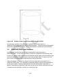
Component Insertion icon feature menus ....................................................... 3-46
Cylinder drawn using the Annotation features of SNAP.................................. 3-47
RCS activity calculator window ...................................................................... 3-52
RCS Activity Inputs – PWR window ............................................................... 3-53
RCS Activity Inputs – BWR window ............................................................... 3-54
Calculate Iodine Activity window .................................................................... 3-55
Available pre-defined SNAP/RADTRAD release models ................................ 3-56
Linkage of a dose location and Χ/Q table for a compartment ......................... 3-68
Schematic of a typical SNAP/RADTRAD dose assessment model .................. 4-2
viii
LIST OF TABLES
Table
Table 3-1
Table 3-2
Table 3-3
Table 3-4
Table 3-5
Table 3-6
Table 3-7
Table 3-8
Table 3-9
Table 3-10
Table 3-11
Table 3-12
Table 3-13
Table 3-14
Table 3-15
Table 4-1
Table 4-2
Table 4-3
Table 4-4
Table 4-5
Table 4-6
Table 4-7
Table 4-8
Table 4-9
Table 4-10
Table 4-11
Table 4-12
Table 4-13
Page
Files available for viewing using the file viewer in the job status window ........ 3-14
Summary of Model Editor menu commands................................................... 3-25
Icons used in the View / Dock window ........................................................... 3-32
Sample problem X/Q values .......................................................................... 3-36
Summary of SNAP/RADTRAD inputs – Model Options .................................. 3-49
Summary of SNAP/RADTRAD inputs – Nuclear Data .................................... 3-56
Summary of SNAP/RADTRAD inputs – Sources............................................ 3-57
Summary of SNAP/RADTRAD inputs – Compartments ................................. 3-58
Summary of SNAP/RADTRAD inputs – Pathways ......................................... 3-59
Summary of SNAP/RADTRAD inputs – Natural Deposition ........................... 3-62
Summary of SNAP/RADTRAD inputs – Filters ............................................... 3-63
Summary of SNAP/RADTRAD inputs – Sprays ............................................. 3-64
Summary of SNAP/RADTRAD inputs – Dose Locations ................................ 3-67
Summary of SNAP/RADTRAD inputs – Χ/Q Tables ....................................... 3-68
Summary of SNAP/RADTRAD inputs – Remaining Nodes ............................ 3-69
Local error solutions for I-131 and I-132........................................................... 4-8
Chemical element grouping for SNAP/RADTRAD .......................................... 4-10
Release phase durations for PWRs and BWRs ............................................. 4-12
Gap release fractions used in SNAP/RADTRAD ............................................ 4-12
SNAP/RADTRAD release fractions for an REA-CRDA accident .................... 4-13
Formulations used to determine RCS water radionuclide concentrations
in PWRs with U-tube steam generators ......................................................... 4-15
RCS radionuclide concentrations for a reference PWR plant ......................... 4-16
Formulations used to determine RCS water radionuclide concentrations
in BWRs......................................................................................................... 4-17
RCS radionuclide concentrations for a reference BWR plant ......................... 4-18
Values for coefficients used in the Powers’ spray removal model .................. 4-21
Correlations of natural deposition decontamination coefficients for PWRs
DBAs ............................................................................................................. 4-25
Correlations of natural deposition decontamination coefficients for BWRs
DBAs ............................................................................................................. 4-26
Correlations of natural deposition decontamination coefficients for APWR
DBAs ............................................................................................................. 4-27
ix
ACKNOWLEDGMENTS
Many people, both with the U.S. Nuclear Regulatory Commission as well as at contractor
organizations have contributed to the development of SNAP/RADTRAD. The individual who
has provided unflagging support for the development of SNAP/RADTRAD over the past several
years is Mark Blumberg from the Office of Nuclear Reactor Regulation. Mark has been the
Technical Monitor for the RADTRAD code’s design, computational methods and testing since
1997. He has also provided much insight into dose analysis for licensing applications
throughout the code’s conversion to the JAVA computer programming language and the entire
SNAP/RADTRAD development process. The agency would like to recognize Chester Gingrich
from the Office of Nuclear Regulatory Research who was responsible for the initial conversion
and code programming of RADTRAD into JAVA. Another individual who is acknowledged is
Stephen LaVie from the Office of Nuclear Security and Incident Response whose development
of the RNEditor code is a key element of the source term modeling approach used in
SNAP/RADTRAD. Finally, the support of John Tomon of the Office of Research who is the
current Contracting Officer’s Representative and whose patience and guidance is greatly
appreciated.
In the contractor organizations, the contributions of Ken Jones of Applied Programming
Technology who, along with his programming staff, develop and maintain the SNAP code are
greatly appreciated.
xi
ABBREVIATIONS
APT
AptPlot
APWR
Bq
BWR
Ci
CRDA
DCF
DE
DE I-131
DE Xe-133
DF
DBA-TID
DBA-AST
EAB
FGR
FHA
GUI
HEPA
LOCA
LPZ
MWth
NRC
ODE
PWR
RCS
RADTRAD
RAMP
REA
RG
SI
SNAP
Sv
TEDE
T/S
XML
Applied Programming Technology
Applied Programming Technology plotting package
advanced pressurized-water reactor
Becquerels
boiling-water reactor
curie
control rod drop accident
dose conversion factor
dose equivalent
dose equivalent iodine 131
dose equivalent xenon 133
decontamination factor
design-basis accident based on TID-14844
design-basis accident using NUREG-1465 (Regulatory Guide 1.183)
models
exclusion area boundary
Federal Guidance Report
fuel handling accident
graphical user interface
high-efficiency particulate air
loss-of-coolant accident
low population zone
megawatt thermal
U.S. Nuclear Regulatory Commission
ordinary differential equation
pressurized-water reactor
reactor coolant system
RADionuclide Transport, Removal, And Dose Esitmation
Radiation Protection Computer Code Analysis and Maintenance Program
rod ejection accident
Regulatory Guide
International System of Units
Symbolic Nuclear Analysis Package
Sieverts
total effective dose equivalent
technical specification
extensible markup language
xiii
1.0
INTRODUCTION
The purpose of the Symbolic Nuclear Analysis Package/RADionuclide Transport and Removal
and Dose Estimation (SNAP/RADTRAD) code is to determine the dose from a release of
radionuclides during a design basis accident to the exclusion area boundary (EAB), the low
population zone (LPZ), and the control room and other locations of interest. As radioactive
material is transported through the containment, the user can account for sprays and natural
deposition to reduce the quantity of radioactive material. Material can flow between buildings,
from buildings to the environment, or into control rooms through high-efficiency particulate air
(HEPA) filters, piping, or other connectors. Decay and in-growth of daughters can be calculated
over time as the material is transported.
The focus of SNAP/RADTRAD is licensing analysis to show compliance with nuclear plant siting
and control room dose limits for various loss-of-coolant accidents (LOCAs) and non-LOCA
accidents. The RADTRAD code was originally developed by the Accident Analysis and
Consequence Assessment Department at Sandia National Laboratories for the U.S. Nuclear
Regulatory Commission (NRC) in 1997 as documented in NUREG/CR-6604, “RADTRAD: A
Simplified Model for RADionuclide Transport and Removal and Dose Estimation,” [1]. The code
was revised to include a Visual Basic graphic user interface (GUI) for user convenience in 1999,
which is described in NUREG/CR-6604, Supplement 1, “RADTRAD: A Simplified Model for
RADionuclide Transport and Removal and Dose Estimation,” [2]. Finally, NUREG/CR-6604,
Supplement 2, “RADTRAD: A Simplified Model for RADionuclide Transport and Removal and
Dose Estimation,” [3] was published in 2002 discussing the testing of RADTRAD version 3.03.
The NRC decided to update RADTRAD by converting the code into JAVA and develop a
RADTRAD plugin to interface with the SNAP graphical user interface (GUI). As part of the
RADTRAD update, the analytical code that calculates the doses and generates the results was
separated. Hence, SNAP with the RADTRAD plugin is used to develop models and prepare
input which is then processed by the RADTRAD analytical code (RADTRAD-AC). The
RADTRAD-AC then calculates the dose and generates the results. The combined package is
referred to as SNAP/RADTRAD. Use of RADTRAD in the SNAP framework allows use of the
SNAP features including the Model Editor for developing plant models. The Model Editor also
provides tools for user input checking, for submitting and monitoring calculations, and for
running multiple cases. The RADTRAD-AC generates data output files suitable for plotting with
the Applied Programming Technology plotting package (APTPot).
As part of the development of the RADTRAD plugin for SNAP, the user documentation is being
updated. This report provides the documentation for the use of SNAP/RADTRAD.
1-1
2.0
INSTALLATION GUIDE
This section of the report discusses how to obtain and install SNAP/RADTRAD and the
RADTRAD-AC codes.
2.1
Distribution
RADTRAD is distributed in two parts: the SNAP GUI with the RADTRAD plugin and the
RADTRAD-AC. SNAP with the RADTRAD plugin is used for model development and input
preparation while the RADTRAD-AC carries out the calculations and generates the results.
SNAP with the RADTRAD plugin is maintained by Applied Programming Technologies, Inc.
(APT) and the RADTRAD-AC analytical code is maintained by Information Systems Laboratory,
Inc.
Directions for obtaining the SNAP GUI with the RADTRAD plugin and the RADTRAD-AC are
available at the Radiation Protection Computer Code Analysis and Maintenance Program
(RAMP) website. Current version information for SNAP with the RADTRAD plugin and
RADTRAD-AC are also available at the RAMP website. Note that results plotting capability has
been built into SNAP/RADTRAD using the AptPlot program.
The SNAP GUI with the RADTRAD plugin and the AptPlot program is available from the APT
website. The RADTRAD-AC analytical code is available from the RAMP website. This code is
designed to be compatible with the SNAP GUI with the RADTRAD plugin.
2.2
Hardware and Software Requirements
The SNAP GUI with the RADTRAD plugin (SNAP/RADTRAD) and the RADTRAD-AC code can
be executed on any computer that supports Java applications. Any of the current generation of
personal computers that can run the Java runtime environment is capable of running
SNAP/RADTRAD and the RADTRAD analytical code. For a Windows computer, the Windows
versions that can be used are Vista, Windows 7 and Windows 8. It should be noted that the
following software is required:
•
Java Standard Edition (SE) 6.0 or later. This package is currently available on
http://www.oracle.com/technetwork/java/javase/downloads/index.html.
•
SNAP GUI with the RADTRAD plugin code maintained by APT.
•
RADTRAD-AC packaged separately, and distributed by RAMP.
•
APTPlot – plotting package maintained by APT. For further details, see
https://www.appliedprog.com/.
2-1
Although not required, the jedit text editing program adds some user conveniences in
SNAP/RADTRAD. This package is available from www.jedit.org.
2.3
Installation
Installation of SNAP is very similar to installation of any software package on a Windows
system. Basically, directory locations on the hard drive to install SNAP are selected. If not
already accepted earlier, license agreements are then displayed, which the user needs to agree
to before proceeding. During the installation process, windows showing installation process and
user-selectable installation options are displayed.
For SNAP/RADTRAD and AptPlot, a Java-based installer file named snapinstaller.jar is
provided that guides the installation process of SNAP/RADTRAD. Screenshots of the windows
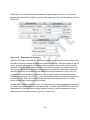
for AptPlot and SNAP/RADTRAD produced by the installation process are presented in Figures
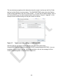
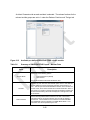
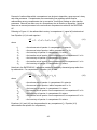
2-1 (AptPlot) and Figure 2-2 (SNAP/RADTRAD).
Figure 2-1
AptPlot installation screens
For AptPlot, the AptPlot Installation Tool, the user interface for AptPlot shows the progress of
the installation. The location of the installation directory is shown in the Installation Directory
window. The user can change the location although the default location is usually adequate.
2-2
After selecting the installation directory, the Java Runtime Environment License Agreement
appears which the user must agree to in order for the installation process to proceed forward.
Once this step is completed, a second license agreement for AptPlot (the GNU General Public
license will appear which again the user must agree to in order to continue.
The user will then be required to select plugins. In the case of AptPlot, the user will select the
analysis code support (ACS) Plug-in and then click on Continue. The installation will proceed to
completion and the user clicks on Close in the AptPlot Installation Tool window to exit the
AptPlot installation.
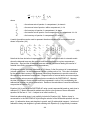
The installation steps for the SNAP/RADTRAD plugin are essentially the same as for AptPlot,
although the windows are somewhat different. The SNAP Installation Tool is the user interface
for SNAP installation which shows the progress of the installation. The location of the
installation directory is shown in the Installation Directory window. The user can change the
location although the default location is usually adequate. After selecting the installation
directory, the Java Runtime Environment License Agreement appears which the user must
agree to in order to continue the installation. Once this step is completed, a second license
agreement for the APT binary code license agreement appears which again the user must
agree to in order to continue.
The user will then be required to select plugins. In the case of SNAP, the user will select the
AVF, ENGTMPL, EXTDATA, RADTRAD, and Uncertainty plug-ins and then click on Continue.
The installation will proceed to completion and the user clicks on Close in the SNAP Installation
Tool window to exit the SNAP installation. If the user wants to know the purpose of each plugin, the user can click on each package name and a description will appear on the right-hand
side of the plug-in manager window as illustrated in Figure 2-2.
The installation files are written to the /users/homedir where homedir is the home directory for
the login ID being used unless you specified a different location. These files are included in the
snap and .snap directories. The code files are written to the snap directory and files needed to
use SNAP on a given system are written to .snap. For example, the location of the root folder
on a given computer is written to the .snap directory. The installation files for AptPlot are also in
/users/homedir in the AptPlot and .aptplot directories. If the user is uncertain of the location of
the home directory is, a command window can be opened by going to Start and typing in
command in the Search textbox (Windows 7). A command prompt window should appear
(select Command Prompt from menu above if necessary). Then, type in echo
%USERPROFILE% and your home directory will be displayed.
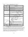
2-3
Figure 2-2
SNAP installation screens
Finally, the RADTRAD-AC should be installed in the radtrad subdirectory under the snap
directory in the /users/homedir. The RADTRAD-AC distribution consists of a group of Java .jar
files that are distributed as a zip file from the RAMP website. These files are castorcodegen.jar, castor-core.jar, castor-xml.jar, castor-xml-schema.jar, commons-logging.jar, and
radtrad.jar. To install these file, create a subdirectory named radtrad in the installation directory
for SNAP/RADTRAD, unzip the files and copy them to that directory. The path to the radtrad.jar
file needs to be set in the configuration tool. Note that the SNAP/RADTRAD installer
automatically defines the path to the RADTRAD analytical code jar file as:
${SNAPINSTALL}/radtrad/radtrad.jar,
so if the aforementioned .jar files are copied to a radtrad subdirectory in the SNAP/RADTRAD
installation directory, the code should be ready for use. The location of this link within the SNAP
framework is discussed in Section 2.2.
2-4
2.4
Sample Problems
A set of sample problems for SNAP/RADTRAD are provided on the RAMP website. These
problems provide a starting point for the user. In addition, there is a Test23 sample problem
provided with the SNAP installation files from APT. This problem is used to illustrate the use of
SNAP/RADTRAD in Section 3.0. The user will also find the information on the QuickStart.pdf
file on the RAMP website to be useful.
2.5
Contact Information
Any questions, suggestions, corrections or comments concerning this the code or its
documentation should be submitted to [email protected] or [email protected].
2.6
Code Error and Problem Reporting
While every effort has been made to minimize errors in SNAP/RADTRAD, there may be
unanticipated circumstances that lead to errors and problems (bugs). To report errors and bugs
with the program, first collect as much information as possible about the error or bug. This
information should include answers to the following questions:
•
•
•
•
•
•
What version of the SNAP/RADTRAD program are you running? The information for
SNAP can be found on the screen displayed at startup or by using the Help | About
menu item. Click the Plugins button at the bottom of the popup screen to get the
information about the SNAP/RADTRAD Plugin.
What computer operating system is SNAP/RADTRAD being executed on?
Is the error or bug reproducible?
What are the steps leading up to the problem?
What are the exact symptoms (e.g. program crash, error message, etc.)?
Save the case files and attach them to an issue report.
To report a problem, send a zip file with the case files and answers to the above questions to
[email protected].
2-5
3.0
MODEL DEVELOPMENT USING SNAP/RADTRAD
To run SNAP/RADTRAD will require some familiarity with the overall SNAP approach to
developing and running models. In this section, the approach to using SNAP to develop, modify
and execute RADTRAD problems will be discussed. However, SNAP includes many features
which will not be discussed here. However, for the interested user, the Symbolic Nuclear
Analysis Package User's Manual [4] provides more detailed information on the use of SNAP.
3.1
Overview of SNAP/RADTRAD
SNAP is actually a suite of computer applications used to develop, modify, and execute
computer models principally for thermal hydraulic codes such as the TRAC/RELAP Advanced
Computational Engine (TRACE) and Reactor Excursion and Leak Analysis Program (RELAP5).
Of these tools, the Configuration Tool, Model Editor and the Job Status tools are most relevant
to RADTRAD analysis. The Configuration Tool is used to configure global properties for running
RADTRAD under SNAP. The Model Editor provides a GUI used to develop RADTRAD models.
The Job Status tool is used to obtain the job status. Of these tools, the Model Editor is the tool
used the most as it is the primary tool for developing SNAP/RADTRAD models.
Generally, the approach for developing a new SNAP/RADTRAD model is to define the
compartments and connections in flow pathways that represent the plant and optionally the
control room and/or the technical support center being analyzed. Note that flow pathways are
used to connect components in SNAP/RADTRAD. During the specification of components and
flow pathways, removal models should be considered and specified for each normal
compartment as appropriate. For compartments, these removal models include filtration,
sprays, or natural deposition. The user will need to specify each model required and specify the
required data using the SNAP GUI as a guide.
Once the geometric, flow/leakage and removal information is specified for the compartments
and flow pathways, a source term is then specified. A comprehensive list of nuclides based on
International Commission on Radiological Protection (ICRP) Report 38 [5] has been included in
SNAP/RADTRAD. The user will need to decide whether the analysis is either being done based
on the occurrence of a LOCA by selecting either TID-14844 or NUREG-1465 or for non-LOCA
where both radionuclides from the fuel and the reactor coolant activity may be important
contributors and make the appropriate selections for the plant being analyzed. A plant power
level must be defined to obtain the correct source term. The iodine physical form must also be
defined as the rate of removal and filtration depends on the physical form of iodine.
Parameters related to the dose rate are specified, including Χ/Q data for each receptor location
and dose conversion factors (DCFs). Default DCFs based on EPA-520/1-88-020, “Limiting
Values of Radionuclide Intake and Air Concentration and Dose Conversion Factors for
Inhalation, Submersion, and Ingestion,” Federal Guidance Report No. 11 (FGR 11) [6] and EPA3-1
402-R-93-081, “External Exposure to Radionuclides in Air, Water, and Soil,” Federal Guidance
Report No. 12 (FGR 12) [7] (see Section 4.6) are built into SNAP/RADTRAD. The EAB and the
LPZ are defined by default in SNAP/RADTRAD. Other dose receptors can be added as
needed. For each dose receptor that is located in the environment or draws from the
environment such as a control room, time-dependent Χ/Q and breathing rate values must be
specified. For the control room, occupancy factors must also be specified. Note that default
values for breathing rates are provided that are suitable for most analyses.
SNAP/RADTRAD can be used to develop new models and modify existing models. The key
aspect of model development is the use of compartments and connecting flow pathways to
model a system. The approach used to prepare this section was to open the SNAP GUI and
start exploring the features for RADTRAD model development. Therefore, the discussion in the
following sections assumes that the user has SNAP available and open and that the user will
follow along with the discussion by using the SNAP/RADTRAD Model Editor. There is no better
way to learn how to use the SNAP GUI except to actually use it.
3.2
The Model Editor User Interface- Model Development
This subsection describes working within the SNAP/RADTRAD Model Editor to develop and
modify models.
3.2.1
Overview of Existing Model Features
As noted earlier, the SNAP/RADTRAD Model Editor is the basic tool used to create, modify and
run input models. To start the Model Editor, navigate to Start->All Programs->SNAP->Model
Editor, and the Model Editor should start.
To illustrate many of the features in SNAP, the Test 23 sample problem will be used. This
problem is found in the Samples/Test23 subdirectory in the snap directory (see Section 2.3). It
is recommended that a copy of the Test23.med file be placed in the user’s working directory,
which is the directory where the input and output files will be kept. It is also recommended that
the user open Test23 and follow along with the presentation in this section.
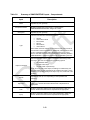
When the Model Editor is started, a splash screen appears for several seconds and then a
Welcome to Model Editor screen appears as shown in Figure 3-1 with the Model Editor window
in the background.
Several options are available on the Welcome to Model Editor screen, which are listed below:
•
•
•
•
Create A New Model
Open a Model Document
Import a New Model
Start an Empty Session
3-2
•
SNAP Version Updates
Under each of these items a short description of each option is provided to explain what each
option does.
Figure 3-1
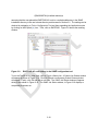
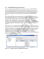
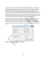
SNAP Model Editor welcome screen
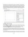
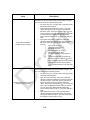
Once the SNAP Model Editor is open, the user selects Continue under Open a Model Document
on the Figure 3-1. Navigate to the location of the Test23 subdirectory under the samples
directory. Click on the file Test23.med. The Model Editor rendering of Test23 will open as
shown in Figure 3-2. Alternately, the user can click on the Test23.med file in the working
directory to start the SNAP Model Editor.
Finally, the model can also be opened by selecting File->Open, navigating to the input file (.med
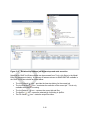
file) of interest, selecting that file and clicking on open, much like any Windows program. Notice
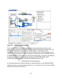
that there are three separate input sections in the SNAP Model Editor window shown in Figure
3-3
3-2 which are: the Navigator window, the Property window and the View / Dock window where
the model rendering appears. Also, notice that there are two tabs in the View / Dock window
labeled Default View and Test23 View. In this model the SNAP/RADTRAD job stream is shown
while the model rendering is shown in the Default View. The tabs can be clicked-on to show
either the modeling rendering or the job stream (similar to Microsoft Excel). Job streams will be
discussed later in this section. There is also a Message window underneath the View / Dock
window which lists messages from SNAP/RADTRAD.
The user should note that each of the windows shown in Figure 3-2 can be resized either
horizontally or vertically. Resizing is done by hovering the mouse cursor over the border
between the windows until a double-headed arrow appears. Then the user clicks and drags the
border to the desired location.
The user will need to unlock the model by clicking on the Lock ( ) icon shown in Figure 3-2.
Notice that other icons adjacent to the Lock ( ) icon will change to unlocked ( ) on the toolbar.
Figure 3-2
SNAP Model Editor screen
One powerful feature in SNAP/RADTRAD is the ability to check the model for input errors. To
illustrate the use of this feature, click on Tools->Check Model to perform a model check. Note
that the message Note: Model check complete. No errors found in the Message window at the
bottom of the screen.
3-4
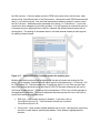
The input groups are shown in the Navigator window. Clicking on the Expand ( ) icon will
expand each group and node, showing the associated input data for that input group and node.
Figure 3-3 presents an illustration of a node expansion which is obtained by clicking on the
Expand ( ) icon next to Compartments, then clicking on Compartment 1. Note that the
Compartment 1 input appears in the Property window (lower left). The user should experiment
with other input groups as the approach is the same. Input specification will be presented later
in this section.
Note that the black bar where the input model name appears (Test23.med) contains some
important features which are summarized in Section 3.4. One of these features is the ability to
switch units from British to International System of Units (SI). Units switching is done by rightclicking on the black bar, selecting Engineering Units->British to change the units from SI to
British.
Figure 3-3
Illustration of the expand icon
3-5
Icons are used to represent the various components used in the View / Dock window that
comprise a typical model. Figure 3-4 presents an illustration of the various icons used.
Figure 3-4
3.2.2
Illustration of the various icons used to represent a SNAP/RADTRAD
model
Job Streams and Case Execution in SNAP/RADTRAD
Before continuing the discussion of existing model features and developing a new model, the
Test23 case will be run to illustrate how cases are run.
Case execution is dependent on the job stream, which are a source of confusion for new
SNAP/RADTRAD users. Simply put, job streams are used to pass input and output data from
one code to another for cases where multiple codes are used. SNAP is used to support a wide
variety of analysis programs that pass data from one program to another. This feature is less of
an issue with SNAP/RADTRAD because in most cases, output from SNAP/RADTRAD
(RADTRAD-AC) is passed to AptPlot for plotting. For the convenience of the user, a default job
stream is predefined for all SNAP/RADTRAD cases.
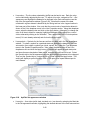
Figure 3-5 presents a typical SNAP/RADTRAD job stream. The default job stream for
SNAP/RADTRAD shows three steps: 1) input preparation shown in the RADTRAD Model
(Base_Model) node, 2) the analytical code execution in the RADTRAD (RADTRAD) node and 3)
3-6
the passing of plot data from SNAP/RADTRAD to AptPlot (PlotStep) node. Input is passed from
the Model Editor (Base_Model) to the RADTRAD analytical code (RADTRAD). The plot file
data generated by the RADTRAD-AC is passed to the AptPlot (PlotStep) node.
Figure 3-5
Typical job stream in SNAP/RADTRAD
As in the case of model input, job streams specification can also be checked. In the case of the
Test23 problem, expand the Job Stream node in the Navigator window; select Test23 and rightclick, then select Check Stream. An error report window will appear in the Message window
and in this case, no errors were found.
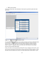
Part of the job stream input specification is to determine where the RADTRAD-AC output will be
written. When the job stream node is expanded as above, the job stream properties appear in
the Property window as illustrated in Figure 3-6.
Figure 3-6
Job stream Property window
3-7
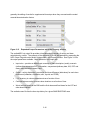
The two job stream properties which determine where the output is written are the Root Folder
text box and the Relative Location text box. The SNAP/RADTRAD output is then the Relative
Folder location appended to the Root Folder location. To review the root folder settings, click on
the Custom Editors ( ) icon and a window similar to that shown in Figure 3-7 appears. In this
example, three root folders along with the path location are shown.
Figure 3-7
Typical root folder settings in SNAP/RADTRAD
Assuming that the root folder is set to Samples, the path to the output will be
Samples\RADTRAD or C:\Work\Current\0-RADTRAD\Training\Samples\RADTRAD. In a new
installation, the root folder is not set. When the root folder is not set, the message No Root
Folders Available appears in red as shown in Figure 3-8.
3-8
Figure 3-8
Job stream Property window with an unset root folder
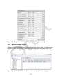
Setting the root folder requires selecting the Custom Editors ( ) icon under the Root Folder text
box to open the Edit Calculation Server Root Folders window. Click on the New ( ) icon and
navigate to the desired location in the Select Folder Location window. The root folder name will
change to the last folder name in the directory path.
The relative location can be reset and should be reset to a name more mnemonic so that the
SNAP/RADTRAD cases can be tracked. For example, to change the name, highlight the
Relative Location Name and type in a new name (Sample to Test23). Note that the file location
is automatically appended.
Note that multiple root folders are allowed which is handy for organizing SNAP/RADTRAD case
files. To add a root folder, navigate to Tools->Job Status or click on the Job Status ( ) icon and
expand Local. Right-click on Local and select Root Folders. Click on the New ( ) icon (left on
Toolbar) and navigate to where you want the root folder (ex. NPP Dose Analysis). The root
folder path will be created. Also, a path of subdirectories can be specified in the Relative
Location text box separated by a back slash ( / ). For example, the relative location can be set
to RADTRAD/LOCA, so that the path to the output would be Samples/RADTRAD/LOCA
assuming that the root folder is set to Samples.
A couple of points should be noted about root folders. First, the root folder directory needs to
exist – otherwise you’ll get a warning that the directory doesn’t exist and the root folder will
not be defined. Second, overlapping paths are not allowed and will generate an error. At this
point, the user can run Test23. However, as a reminder, one item should be checked before
proceeding and that is the link to the RADTRAD-AC. This link should have been set
automatically during the installation process. The setting is:
3-9
${SNAPINSTALL}/radtrad.radtrad.jar,
assuming that the user placed the RADTRAD-AC code in a radtrad subdirectory in the SNAP
installation directory in the user’s home directory as discussed in Section 2.2. The setting can be
checked by navigating to Tools->Configuration Tool and then expanding the Applications node
by clicking on the Expand ( ) icon. Then, click on RADTRAD. Figure 3-9 shows the resulting
window.
Figure 3-9
RADTRAD-AC code setting in the SNAP configuration tool
To run the Test23 or any other case, click on Tools->Submit Job. A Submit Job Stream window
will appear as shown in Figure 3-10. Click on OK and a confirmatory Submit Stream window
will appear. Finally, click OK and the run will start. The SNAP Job Status window will appear
which is also shown in Figure 3-10. The SNAP Job Status window, in Figure 3-10 displays a
completed job stream run.
3-10
Figure 3-10
SNAP/RADTRAD job stream and status windows
The relationship between the SNAP/RADTRAD job stream and the actual case execution is
shown in Figure 3-11. In the upper left-hand corner, the graphical job stream representation is
shown. As noted earlier, this representation shows passing input from the SNAP GUI with the
RADTRAD plugin to the RADTRAD-AC and then to AptPlot. The job stream properties are
shown in the Navigator window shown in the upper-right corner of Figure 3-11. The links
between the various nodes are also shown. In the SNAP Job Status window, the status of each
of the job stream steps is shown. Again three steps are shown. The user interaction with the
SNAP Job Status window will be discussed in Section 3.2.3.
3-11
Figure 3-11
Relationship between job stream steps and code execution
Note that the SNAP Job Status window can be accessed from Tools->Job Status in the Model
Editor for subsequent viewing. A summary of features relevant to SNAP/RADTAD available in
the SNAP Job Status window are listed below:
•
•
•
•
•
The Job Console ( ) icon – provides the time step history for the current job.
The Job Execution ( ) icon – terminates the execution of the current job. This is only
available when the job is running.
The Job Deletion ( ) icon – removes the current job and files.
The AptPlot ( ) icon – opens the selected job for plotting in AptPlot.
The File Viewer ( ) icon – starts the output file viewer.
3-12
3.2.3
SNAP/RADTRAD Input and Output Files
There are a number of files produced that the user should be aware of in SNAP/RADTRAD.
The main SNAP/RADTRAD interface file is the casename.med file where casename is the
name of the case being analyzed. The casename.med file contains the data needed to render
the model in the SNAP GUI, the default data used by the code and the user-specified input
data. Section 3.4 discusses the actual input that can be specified for a SNAP/RADTRAD
model.
When a SNAP/RADTRAD case is executed through the RADTRAD-AC, the data flow is not
directly from the casename.med file. Rather, there are a number of data files that are produced
by the SNAP/RADTRAD plugin that are read by RADTRAD-AC. These files, which are in
extensible markup language (XML) format, include DCFs (.dfx), nuclide data (.nix), plant
information (.psx), release fraction (.srx), and nuclide inventory (.icx) files. Output files (.out,
.screen and .plot) are produced by the RADTRAD-AC. Log files produced by SNAP/RADTRAD
are job stream related files (.streamlog and .taslog). Table 3-1 provides a brief description of
these files.
When case execution is completed, the SNAP/RADTRAD output can be reviewed by clicking on
the File Viewer ( ) icon. Note that there is a context in terms of the active job stream step and
the output that is displayed. If the casename step is highlighted, then the job stream log will be
available for viewing. If the RADTRAD step is highlighted as shown in the SNAP Job Status
window in Figure 3-12, then the RADTRAD-AC output is available. If the PlotStep is
highlighted, then the plot file data can be viewed using AptPlot. Figure 3-12 shows a
screenshot of the dropdown menu cascade from the File Viewer ( ) icon for the RADTRAD job
step from the SNAP Job Status window.
Figure 3-12
Dropdown menus for SNAP/RADTRAD output
3-13
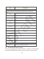
Table 3-1
Files available for viewing using the file viewer in the job status window
Description
File Name
Job Status Window Casename Files
StreamLog - Casename.streamlog
Output from job stream manager. Provides a highlevel summary of the execution steps for the job
stream. Typically not reviewed by the
SNAP/RADTRAD user.
a
Job Status Window RADTRAD Files
Plot Files - > plot - radtrad.plot
c
Text Files - > input – radtrad.psx
Text Files - > nix – radtrad.nix
Text Files - > dfx – radtrad.dfx
Data file for AptPlot from the RADTRAD-AC.
Plant data input file in XML format. Includes the plantspecific data specified by the user including model
parameters, information for plant geometry for each
compartment, information for each flow path, dose
point information including Χ/Q and breathing rates,
occupancy factors, and information for various
radionuclide removal models (sprays, natural
deposition, and filters).
b
Nuclide data information from ICRP-38 in XML format.
Includes the atomic mass, half-life (s), and branching
ratios for radionuclide daughters.
b
DCF file in XML format based on FGR 11 and 12 (see
Section 4.6). Includes the organ-specific DCFs. Note
that only the cloudshine (immersion) and the inhaled
chronic [total effective dose equivalent (TEDE)] and
skin DCFs are used to determine dose. Organspecific factors as well as those factors for
groundshine, inhaled acute and ingestion are not
used.
b
Text Files - > icx_1 – radtrad_1.icx
b
Text Files - > icx_2 – radtrad_2.icx
b
Initial radionuclide inventory file in XML format.
(etc.)
Text Files - > srx_1 – radtrad_1.srx
b
Text Files - > srx_2 – radtrad_2.srx
b
Release fraction information file for each radionuclide
group.
(etc.)
Text Files - > output – radtrad.out
Text Files - > NRC-out – radtradNRC.out
Text Files - > log – radtrad.log
a
Output file from the RADTRAD-AC in the original
format.
c
c
Output file from the RADTRAD-AC in the revised NRC
format.
Debug output (usually not referred to by the user).
3-14
Description
File Name
Text Files -> screen – radtrad.screen
Problem time output to show progress of a given
case.
c
Text Files -> Task Log – RADTRAD_tasklog
a
Output from SNAP job steam showing RADTRAD job
step execution information (usually not referred to by
the user).
Job Status Window PlotStep Files
PDF Documents – time_pdf – time.pdf
c
Time step results (usually not referred to by the user).
Text-Files -> screen – aptplot.screen
Screen output from AptPlot (usually not referred to by
the user).
Text-Files -> Task Log – PlotStep.tasklog
Output from SNAP job steam showing AptPlot job
step execution information (usually not referred to by
the user).
a. SNAP/RADTRAD specific output.
b. Input file to the RADTRAD-AC analytical code generated by SNAP/RADTRAD plugin.
c. Output file from the RADTRAD-AC analytical code.
The files produced by the RADTRAD-AC code which are radtrad.out, radtradNRC.out,
radtrad.plt, and radtrad.screen are the most relevant to the user. The radtrad.out file is basically
the original (Version 3.03/3.10) output file. Major sections of this output file are:
•
Input listing – provides a listing of the input in XML format that is used by the RADTRADAC.
•
Input echo – provides an edited input summary of plant description (model), scenario
(radionuclide source term/DCF) information, compartment/pathway data, Χ/Q, DCF and
decay data, and other relevant input.
•
Breakdown of dose results and nuclide inventory in various compartments at various
time points generally selected by changes in events (i.e. time at which flow rate
changes, and time at which Χ/Q changes). Activity balance information is also given.
•
I-131 inventory in various compartments as a function of time.
•
Cumulative dose results at various dose locations as a function of time.
•
Worst two-hour doses at the EAB and the final doses and final doses for the LPZ and
other dose locations.
The output contents can be controlled from Model Options node by expanding the Output
Parameters tab in the Property window (Figure 3-130. The main difference in the output is
3-15
generally the editing of results for supplemental time steps when they are used and the model
removal/decontamination factors.
Figure 3-13
Expanded Output Parameters tab in the Property window
The radtradNRC.out output file provides a time-dependent summary of activity and dose
calculations by nuclide. The contents of the radtradNRC.out file are controlled by expanding the
NRC Output Flags tab under Model Options node in the Property window. See Figure 3-14 for
the output parameters available. Major sections of this output are:
•
Input echo – provides an edited input summary of plant description (model), scenario
(radionuclide source term/DCF) information, compartment/pathway data, Χ/Q, DCF and
decay data, and other relevant input.
•
Output – activity distribution, cumulative and dose difference (delta-dose) for each dose
component (inhalation, cloudshine, skin, thyroid, and TEDE).
•
I-131 inventory in various compartments as a function of time.
•
Cumulative dose results at various dose locations as a function of time.
•
Worst two-hour doses at the EAB and the final doses and final doses for the LPZ and
other dose locations.
The radtrad.screen file lists the time step history for a given SNAP/RADTRAD case.
3-16
Figure 3-14
3.2.4
Expanded NRC Output Flags tab in the Property window
AptPlot Plotting Program
A feature of SNAP/RADTRAD is the ability to display plots of dose results. To display a plot,
click on Plot Files and select plot – radtrad.plt. AptPlot will open. Alternately, click on the
AptPlot ( ) icon in the SNAP Job Status window and AptPlot will open as illustrated in Figure 315.
Figure 3-15
SNAP/RADTRAD Job Status window with AptPlot icon highlighted
3-17
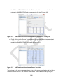
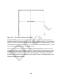
When AptPlot opens, the windows presented in Figure 3-16 will appear. Dose information by
dose location (ExclusionAreaBoundary, LowPopulationZone, and ControlRoom spaces omitted)
and dose category (body, cloudshine, skin, tede, and thyroid) for each nuclide separated by
periods will be presented in the Select EXTDATA Channels window in Figure 3-17. In AptPlot,
each data set is referred to as a data channel. Test Problem 23 is used to illustrate the features
of AptPlot and it is suggested that the user open AptPlot for Test Problem 23 and follow the
discussion below.
Figure 3-16
AptPlot startup view
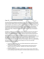
Basically to make a plot, the user scrolls to the result of interest, highlights that result, clicks on
the Plot button and the plot will appear. Note that the default time units are in seconds, but that
can be changed to hours in the dropdown menu next to Time Units text box on the Select
EXTDATA Channels window (Figure 3-17) prior to actually generating the plot.
AptPlot has many features for generating and formatting plots and the discussion presented
here is not meant to be exhaustive. A comprehensive help manual can be obtained by selecting
Help->Help Contents from the top menu. However, some of the more commonly used features
are illustrated here.
As the user gains familiarity with the naming convention, the filter feature can be used to locate
specific results of interest by entering the dose location, dose category, and nuclide of interest in
3-18
the Filter text box. If the user wants to plot the TEDE dose results for the control room, enter
the text string ControlRoom.tede* in the Filter text box. Note that the total TEDE dose ends with
tede (i.e. no nuclide is listed). Also note that the asterisks (wildcard) symbol is used to control
the list of all items. Wildcards can be embedded in the string (i.e. ControlRoom.*.I*) to list the
control room dose categories for all iodine nuclides. It is very important to note that the case of
a character counts in applying filters in AptPlot, otherwise the wildcard search feature will not
work properly. The spelling of the dataset name in the data channel window provides a guide
for spelling a channel name.
Figure 3-17
Select EXTDATA Channels window for multiple plots
Multiple data results can be plotted by highlighting the data of interest and clicking the Plot
button. As an example, suppose the user wants to plot the thyroid dose for I-131 through I-135
for Test Problem 23. The user would enter ControlRoom.thyroid.I* in the Filter text box, then
select the resulting data channels in the Select EXTDATA Channels window and click on the
Plot button to make the plot. This string can be shortened to C*R*th*I* as a further example of
the application of wildcards. To select multiple data channels requires the use of shift-click or
control-click feature as described below:
•
Shift-click – used to select a range of datasets. In this case, click on
ControlRoom.thyroid.I131. Then hold down the shift key and select
ControlRoom.thyroid.I135.
•
Control-click – used to select multiple datasets one at a time. Hold down the control key
and click on each dataset, selecting that dataset. Each dataset is highlighted after
selection.
3-19
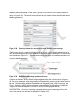
With either approach, all of the dose datasets will be highlighted as shown in Figure 3-17. Once
the datasets are highlighted, click on the Plot button and the plot will be generated. The
resulting plot is shown on Figure 3-18.
Figure 3-18
Control room dose plots for Test23
Adjustments can be made to the plot by using the plot editing features in AptPlot. These
features are accessed by selecting Plot in the top menu. A number of features are available,
but generally Plot->Graph appearance, Plot->Set appearance and Plot->Axis properties provide
the features needed to edit the plot. Screenshots of each of these windows are shown in
Figures 3-19 through 3-21. Clicking on the tabs in each window shows various properties and
features available to the user. A subset of these features is used to edit the plot.
Some typical AptPlot adjustments are illustrated below:
3-20
•
Change the x-axis scale from seconds to hours: – Navigate to the Select EXTDATA
Channel window shown in Figure 3-17 and click on Clear Sets in the lower left-hand
portion of the screen. Then change the units in the Time Units dropdown menu from
Seconds to Hours. Confirm that the dose components are highlighted as shown in
Figure 3-17 using shift-click or control-click. Then, click on Plot and Time (hours) will
appear on the x-axis.
•
Reset y-axis to logarithmic scale: – Given that the I-131 dose is so dominant, it is hard to
read the dose contributions from the other iodine nuclides. The y-axis scale can be
changed to logarithmic by navigating to Plot->Axis properties. Change the axis setting in
Edit text box from X axis to Y axis and click on the Main tab if it is not already selected in
the Axes window (Figure 3-19). Then change the Scale text box from Normal to
Logarithmic and click the Apply button to change the y-axis to logarithmic.
•
Expand y-axis to cover dose range: – The dose range can be expanded from the Axes
window by changing the Start and Stop values to 0.0001 and 10.0. Click on the Main
tab if it is not already selected. Then, enter 0.0001 in the Start text box and 10.0 in the
Stop text box. Then click the Apply button to apply the change.
•
Use scientific notation for the y-axis: – The format for the y-axis labels is set by changing
the Edit dropdown menu setting in the General section of Figure 3-19. Then, set the
number format in the Format dropdown menu in the Tick properties section to Scientific
from General. Also set the precision to 0 in the Precision dropdown menu and click the
Apply button to reset the format.
Figure 3-19
AptPlot Axes window
3-21
•
Line colors: – The line colors selected by AptPlot can be hard to see. Each line color
can be individually adjusted by the user. To adjust a line color, navigate to Plot - >Set
appearance and highlight the dataset to be changed in the Data sets section near the
top of the Set appearance window (Figure 3-20). Note that the name of the data
contained in a given dataset is identified by the String text box in the Legend section in
the lower part of the window. Also, note that the current color of a particular dataset is
shown in the Color dropdown menu in the Line Properties section. Using that dropdown
menu, select the desired color and click on the Apply button. Alternately, to change the
color of all lines to black for example, highlight all datasets using shift-click or controlclick or alternately clicking on the All button. Then, select Black in the Color dropdown
menu (if it is not already selected) and click on the Apply button.
•
Line symbols: – Symbols for the lines are set from the Main tab in the Set appearance
window. To select a symbol for a particular data set, highlight the dataset in the Data
sets section, then select a symbol type (circle, square, etc.) under the Type dropdown
menu in the Symbol Properties section. Also, select the desired color in the Color
dropdown menu and click the Apply button. A symbol will appear for each data point
and since there are hundreds of data points, a symbol skip will have to be set. Select
the Symbols tab in the Set appearance window and highlight the dataset to be changed.
Then, set the Symbol skip to a value like 50 or 75 and click on the Apply button. This
setting will display a symbol for every 50th or 75th point, then repeat these steps for
each dataset.
Figure 3-20
•
AptPlot Set appearance window
Line style: – Line styles (solid, dash, dot-dash, etc.) can be set by selecting the Main tab
in the Set appearance window, highlighting the desired data set in the Data sets sections
3-22
and selecting the desired style using the Style dropdown menu in the Line Properties
section in a manner similar to setting line colors and line symbols. Each line is set
individually, then click the Apply button as the settings for each dataset are completed.
•
Titles and subtitles: – To add a title and subtitle to the plot, select the Main tab in the
Graph appearance window (Figure 3-21). Enter a title and subtitle as appropriate, then
click on the Apply button. The title and subtitle will appear. Select the Titles tab and use
the sliders to adjust the font size for the title and subtitle as desired. Note the font size
can be incremented by clicking on the channel to the left or right of the slider icon.
Figure 3-21
AptPlot Graph appearance window
Sometimes the legend box overwrites the dose results as in the plot shown in Figure 3-16. In
order to correct this issue, the plot needs to be shrunk, which will require using several AptPlot
features. These features are listed below:
•
Edit the legend titles: – The title for each legend can be edited. This change is made by
going to the Set appearance window (Figure 3-20) and highlighting the desired data set.
Change the title in the String text box in the Legend section as appropriate. In this case,
the iodine nuclide name is used. Click on the Apply button after each title modification is
made.
•
Change the font size for the legend: – First, the font size used in legend box will need to
be reduced, which entails changing the legend title font and the symbol font. To change
the font size of the legend title, navigate to the Graph appearance window (Figure 3-21)
and select the Legends tab. Then, use the slider bar to adjust the font size to 75 for
example and click on Apply button. The font size will change for all datasets. For the
symbol size, navigate to the Set appearance window (Figure 3-20) and select all
3-23
datasets. Then, change the Size setting in the Symbol Properties section to 75 using
the slider.
•
Change the size of the plot: – The plot overlays a white background which is basically
set to allow a plot to be printed on 8.5 x 11 paper in landscape mode. So, it is desirable
to maintain this setting although it can be changed by navigating to View->Page setup.
However, the approach used here is to shrink the plot by adjusting the settings in the
Viewport section in the Graph appearance window (Figure 3-21) by entering suitable
values. In this case, the X max and Y max text box settings are changed to 1.0 and 0.8,
respectively. These settings permit the legend box to be moved to the right-hand side of
the plot, then click on the Apply button. Then, to move the legend box, select the Leg.
Box tab in the Graph appearance window (Figure 3-21) and adjust the box location in
the X and Y text boxes in the Location section. Values of 1.05 and 0.60 will move the
legend box to the right-hand side of the plot. Another approach is to change the X max
text box setting to 1000 which will allow sufficient space for the legend box within the plot
frame, although it will probably need to be moved for aesthetic reasons.
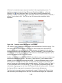
The plot is saved by navigating to File->Save, navigating to the desired directory location,
entering a suitable name, then click on OK, similar to any Windows program. To access a
previously saved AptPlot plot, navigate to File->Open, and navigate to the directory location
where the plot file is saved and select that file. Also, the format and title settings can be saved
by navigating to Plot->Save defaults and overwriting the Defaults.agr file. Note that Plot->Reset
defaults will reset the defaults to the original settings. Figure 3-22 shows the resulting plot with
the above modifications.
Figure 3-22
Reformatted control room dose plots for Test23
3-24
Note that plots can be generated in a picture format such as .png or .jpeg by navigating to File>Print setup. At the top of the Device setup window, change the device to .png for example. In
the Output section, check that the directory path and filename are suitable. Then, click on the
Print button and the plot will be saved in .png format using the filename set for the plot file.
For those users who wish to use a spreadsheet for data analysis or for plotting, the dose data
can be exported. The easiest way is to initiate a new plot session in a comma-delimited format
that can be read by Microsoft Excel. This feature is accessed from the Select EXTDATA
Channels window. As an example, set up and apply a filter for the I-131 to I-135 thyroid dose in
the control room and select the resulting data channels as done previously. Then, highlight the
data channels and click on the Export button at the bottom of the window. A Save window will
appear. Provide a filename, ending the filename with the .csv suffix and select comma
separated values (CSV) as the file type (right hand side of the Save window). Then, click on
Save to write the file. Microsoft Excel will read and organize the dose data by column for
subsequent use.
3.3
SNAP/RADTRAD Model Development and Modification
Sections 3.1 and 3.2 introduced the SNAP/RADTRAD Model Editor user interface using Test
Problem 23 as an example. In this section, the details of building a new model are presented.
For this illustration, a model consisting of a simple containment compartment, leakage pathway,
source and an environment compartment will be developed.
3.3.1
Model Editor Menus
The commands available in the Model Editor are typical of Windows programs. Across the top
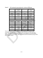
of the Model Editor, the File, Edit, Tools, Window, and Help commands are presented. Table 32 describes the commands associated with each of these menu items.
Table 3-2
Summary of Model Editor menu commands
Description
Menu Command
File Commands
File->New
Creates a new model. A Select Model Type menu appears with
available models listed. The SNAP/RADTRAD user picks RADTRAD
and clicks on the OK button.
File->Open
Opens a previously developed model (.med file). The user navigates
to the directory where the file is located and selects the file to be
opened similar to any Windows program.
File->Open Recent
Allows the user to open a recently used SNAP/RADTRAD model (or
AVF file). The user selects the file of interest and it will open in a new
Model Editor session.
3-25
Description
Menu Command
File->Save
File->Save As
File->Close
File->Close All
Saves the current model with the same name as in any Windows
program.
Saves the file under a new filename. The user navigates to the desired
directory location and/or updates the filename and clicks the Save
button as in any Windows program.
Closes the current model. Provides a warning to the user in the case
of any unsaved changes made to the model.
Closes multiple open models. Provides a warning to the user in the
case of any unsaved changes made to the model.
File->Import
Imports a previously exported RADTRAD model from a set of ASCII or
XML input files (see Section 3.2.3). Note that a .psf file is an ASCII file
with the same input data as the XML formatted .psx files.
File->Export
Exports a set of SNAP/RADTRAD XML input files (.psx, .nix, .srx, .icx,
and .dfx) to a directory selected by the user (see Section 3.2.3).
File->Exit
Exits the Model Editor.
Edit Commands
Edit->Undo
Reverses previous user inputs to a model similar to any Windows
program.
Edit->Redo
Redoes a previous undo command similar to any Windows program.
Edit->Preferences
Allows the user to set various preferences related to fonts, colors, and
other Model Editor features.
Edit->Plugin Manager
Allows enabling and disabling of various plugins. Generally not used
for SNAP/RADTRAD.
Tools Commands
Tools->Check Model
Provides a check of the SNAP/RADTRAD input model. This feature is
very useful for model development in SNAP/RADTRAD.
Tools->Submit Job
Submits a job through the job stream and starts the SNAP Job Status
Tool (see Section 3.2.2).
Tools->Steam Tables
Tools->Configuration Tool
Not used in SNAP/RADTRAD.
Starts the SNAP/RADTRAD Configuration Tool (see Section 3.1).
Tools->Job Status
Starts the SNAP/RADTRAD SNAP Job Status window (see Section
3.2.2).
Tools->Model Note Viewer
Displays model notes. The user can set up and edit notes as part of
the model documentation.
3-26
Menu Command
Description
Tools->Export to jEdit
Exports a model to the jEdit editing program. This feature requires the
installation of jEdit.
Windows Commands
Windows->Commands
Scripting commands window – not used in SNAP/RADTRAD.
Help Commands
Help->Contents
Link to the SNAP Model Editor manual, which includes information
about the RADTRAD Plugin.
Help->Check for Updates
Checks for updates at the APT, Inc. website. Note that computer
security settings may inhibit this feature.
Help->Report an Issue
Allows the user to submit Issue Reports on SNAP/RADTRAD directly
to APT, Inc. Note that issues related to the RADTRAD-AC should be
reported via email to [email protected].
Help->About
Provides information on the SNAP GUI and Plugin version, licensing
agreements, and contact information. Note that plugin version
numbers can be obtained by clicking on the Plugins button.
Figure 3-23 shows the icon arrangement and function of each icon in the Model Editor. Of
particular interest is the ability to separate the Navigator, Property, and View / Dock windows
into separate windows and to also arrange the windows vertically by clicking on the
Single/Multiple Windows Modes icons shown in Figure 3-23. The remaining icons provide a
shortcut to some of the menu commands listed in Table 3-2.
Figure 3-23
Model Editor tool bar icon description
3-27
Figure 3-24 shows the icon arrangement and the function for each icon in the Navigator window.
Basically, these tools aid the user in navigating component nodes in the Navigator window and
multiple models in the SNAP GUI.
Figure 3-24
3.3.2
Navigator window tool bar icon description
Building a SNAP/RADTRAD Model – Component Specification
The first step is to start the SNAP Model Editor and click on Create a New Model in the
Welcome screen (Figure 3-1). Select RADTRAD model in the Select Model Type screen that
subsequently appears similar to Figure 3-2 except there are no icons in the View / Dock
window. The basic model nodes are shown in the Navigator window. Expand the Compartment
[1] node using the Expand ( ) icon in the Navigator window. Highlight (click on) the
Compartment 1 (Environment) node, so that data fields for this compartment will appear in the
Property window. Note that an environment compartment is defined by default.
The basic approach to building a SNAP/RADTRAD model is to set up an array of
compartments, flow pathways and specify key parameters in the various components of the
model. For sources, compartments, and pathways that ultimately appear in the View / Dock
window, the basic pattern is to highlight (select) the component category (i.e. Source,
Compartments and Pathways), right-click on the component category, and select New from the
menu to add a numbered component to that component category. These steps result in a new
model component being created.
A new compartment is added by right-clicking on the Compartment node in the Navigator
window and selecting New in the menu that appears. A new compartment component
Compartment 2 is created. Components are not automatically added to the View / Dock
window, but must be added by the user. The new component (Compartment 2) is added to the
3-28
View / Dock window by right-clicking on the Compartment 2 and selecting Add to View->Default
View. Compartment 2 now appears in the View / Dock window.
The new component (Compartment 2) is unnamed. To add a name to the component, type a
name (i.e. Containment) in the Name text box in the Property window. The name will
simultaneously appear in both the Navigator and View / Dock windows [Compartment 2
(Containment)]. Alternately, newly-defined components can also be dragged from the Navigator
window to the View / Dock window by clicking on the component of interest and dragging it by
holding the left mouse button down and moving the cursor to the View / Dock window.
The pre-defined Environment compartment is added to the View / Dock window in a manner
similar to Compartment 2 (Containment) above. Right-click on Compartment 1 (Environment)
and select Add to View->Default View or drag the component by clicking on the new component
node and dragging it into the View / Dock window. The environment compartment will appear in
the View / Dock window. Note that two dose locations (EAB and LPZ) are automatically
specified with the environment compartment.
The next step is to define a flow pathway which is done by right-clicking on the pathway group
node (Pathways [0]) and selecting New in the menu that appears. Pathway 1 appears. Add
Pathway 1 to the View / Dock window by right-clicking on Pathway 1 and then selecting Add to
View Default View as was done above. The flow pathway should be named by entering a
suitable name in the Name text box in the Property window (i.e. Leakage).
Similarly a source can be added by right-clicking on the Sources node in the Navigator window
(Sources [0]) and selecting New. After naming the component (i.e. Fuel Release), the
component can be added to the View / Dock window in the same manner as used above for
compartments and flow pathways.
At this point, the user can see that a pattern is emerging. Each input group has an associated
group node where components within that group can be defined and added to the Navigator
window. Figure 3-25 displays the Navigator window for the components added in the previous
steps above. The component nodes that can be added as part of a model are: Sources,
Compartments, and Pathways. The nodes for Dose Locations, Natural Deposition, Filters,
Sprays, and Χ/Q Tables are not drawn, but are defined in the same manner as compartments,
pathways, and sources by right-clicking on the component group node and selecting New.
3-29
Figure 3-25
Navigator window with newly added model components
At this point, the user has developed a new model consisting of a source, a compartment
representing the containment, a leakage pathway and an environment compartment. Also, this
new model was added to the View / Dock window by either dragging the new component node
to the View / Dock window or right-clicking on the new component node, then selecting Add To
View. Figure 3-26 shows the View / Dock window with the new model’s components.
Additionally, once the components are added to the View / Dock window, they will be needed to
be moved around for presentation clarity. Make sure the Selection Tool ( ) icon is activated
before rearranging the icons in the View / Dock window. Features common to most Windowsbased programs are available to aid the user in editing and arranging icons. The function of
each icon can be determined by hovering the mouse pointer above the icon of interest. This
action should cause a text pop-up to appear with a short statement of the function of that icon.
The tools and features most commonly used in SNAP/RADTRAD are illustrated in Section
3.3.4.
3-30
Figure 3-26
View / Dock window for 4-node model (unconnected)
Table 3-3 shows all of the icons which are available in the View / Dock window with a
description of each icon. All of the icons for the compartments, sources and pathways have
connection points for connecting flow pathways and source components to compartment
components as illustrated in Figure 3-26. The number in the different icons in Figure 3-26 are
the component number, which are generally consecutive in SNAP/RADTRAD models.
One feature that the user should be aware of is the orientation feature for flow pathway icons.
In Figure 3-26, the orientation is pointing right; however, the orientation can be changed to
pointing up, pointing down, or pointing left by right-clicking on the flow pathway icon and
selecting Drawn Orientation from the menu that appears and then pick the desired orientation.
3-31
Table 3-3
Icons used in the View / Dock window
Description
View / Dock Window Icons
Flow pathway connection point indicated by small circles on
each edge. Small square at the upper-left corner is a source
connection point.
Compartment Icon
Small square at the lower edge is a source connection point to a
compartment.
Source Icon
Flow pathway connection point indicated by small circles on
each side.
Flow Pathway Icon
Flow pathway connection point indicated by small circles on
each edge. Small square at the upper-left corner is a source
connection point.
Environment Icon
Icon denoting that natural deposition is active in a component
(grayed-out indicates inactive).
Icon denoting that a filter is defined in a component (grayed- out
indicates no filter).
Icon denoting that a spray is defined in a component (grayedout indicates no spray).
The next step is to connect the components using the Connection Tool ( ) icon shown in the
View / Dock window tool bar (see Section 3.3.4). Connection points for the various icons are
shown in Figure 3-26. The first step is to click on the Connection Tool ( ) icon in the View /
Dock window tool bar, which activates the connection tool. Then for compartment to flow
pathway connections, click on the connection point (circle) on the edge of the compartment to
be connected and drag holding the left mouse button down to the desired connection point
(circle) on the flow pathway icon and release the button. The procedure is the same for the
source to compartment connections except the connection points denoted by squares are used.
Figure 3-27 shows the model with the connections made.
3-32
Figure 3-27
View / Dock window for 4-node model (connected)
The expanded node view of the Navigator window corresponding to the model in Figure 3-27 is
shown in Figure 3-28. Figure 3-28 shows all of the connections for all of the components shown
in the model. Basically, it is an expanded node view of the schematic representation shown in
Figure 3-25. Users should get into the habit of naming the various components of their models.
This practice will help avoid errors, particularly as models get more complicated.
Figure 3-28
Navigator window with all nodes expanded
3-33
3.3.3
Building a SNAP/RADTRAD Model – Input Specification
Input specification is the next step in developing a SNAP/RADTRAD model. The Model Editor
design basically guides the user through the various input parameters required. Clicking on any
of the defined compartments presents a list of input data that needs to be specified in the
Property window. Also, an important feature in SNAP/RADTRAD is the ability to check the
model using the Check Model feature which is found by either navigating to Tools->Check
Model.
This illustration will start by completing the input for Compartment 2 (Containment) shown in
Figure 3-27. The volume of this compartment will be set to 2.5E+06 ft3. Note that the default
units of the model are in SI. To switch units to English, right-click on the black bar in the
Navigator window, select Engineering Units->British to change the units. Figure 3-29 shows the
location of the black bar and the accompanying menus. Once the units are switched, click on
the Compartment 2 (Containment) icon in the View / Dock window or in the Navigator window
and enter 2.5E6 in the Volume text box in the Property window. Also check that the
Compartment Type text box is set to Normal. Other compartment types are discussed in
Section 3.3.4. Figure 3-30 shows the Property window with the volume set to 2.5E6. Note that
deposition, filter, and sprays models are not used.
Figure 3-29
Navigator window with the black bar menu for the engineering units
selection
Figure 3-30
Property window with volume entry for the Compartment 2 (Containment)
3-34
Input for the flow pathway involves a data entry table to capture the time dependence of the
assumed containment leakage rate of 0.1 percent per day (%/day). The first step is to change
the Pathway Type text box in the Property window from Piping (default) to Air leakage (typically
used for containments). Next, specify a leakage rate by clicking on the Custom Editors ( ) icon
adjacent to the Leakage Rate text box to open the Editing Leakage Rate window Figure 3-31. A
data entry table window will open, which is one of the most common ways to specify input
entries in SNAP/RADTRAD.
Figure 3-31
Pathway input windows for sample problem
The user can click on the Add button and add a leakage rate of 0.1 %/day for 0 to 720 hrs. Two
rows will be needed. Some users prefer to set up the number of rows needed for the data while
others add a new row after each set of data entries are completed. To delete a row, highlight
the row to be deleted and click on the Remove button.
The next step is to specify the Χ/Q tables. The Χ/Q values used for this illustration are listed in
Table 3-4. The approach is basically the same as that used for the flow pathway input. The first
step is to click on the Expand ( ) icon next to the Χ/Q Tables node in the Navigator window,
3-35
then click on Χ/Q Table 1 (Exclusion Area Boundary) node. In the Property window for the Χ/Q
Table 1 (Exclusion Area Boundary) click on the Custom Editors ( ) icon adjacent to the X/Q
Table text box to open the Editing X/Q Table window Figure 3-32. As in the case of the leakage
rate above, the user can enter data in a new table by clicking on the Add button and adding the
values shown in Table 3-4. Using the Add and Remove buttons, the X/Q values for the EAB
and LPZ can be completed by the user. Figure 3-32 shows the completed X/Q tables.
Table 3-4
Sample problem X/Q values
Time Interval
(hrs)
0–2
Figure 3-32
Χ/Q Value by Location
(sec/m3)
EAB
LPZ
1.4E-04
4.5E-05
2–8
2.39E-05
8 – 24
1.29E-05
24 – 96
5.49E-06
96 – 720
1.61E-06
X/Q input tables for EAB (left) and LPZ (right)
3-36
The final item to be completed is the source term specification. The source term specification
consists of two parts. The first part is to specify the radionuclide inventory in the fuel or reactor
coolant and the second is the source or release fraction scenario specific to the accident type.
Both combine to generate the radionuclide inventory to determine an overall source term.
Additionally, there is also the setting for core power in the Model Options node that is used to
determine the radionuclide inventory.
There are two default core inventory libraries (PWR and BWR), which are not editable by the
user, which are used to determine the core inventory.
•
•
PWR – normalized Methods for Estimation of Leakages and Consequences of Releases
(MELCOR) Accident Consequence Code System (MACCS) sample 3412 megawatt
thermal (MWth) PWR core inventory (60 nuclides).
BWR – normalized MACCS sample 3578 MWth BWR core inventory (60 nuclides).
Basic editing features for the Edit Total Inventories window are shown in Figure 3-33. These
features can be used to either edit an existing file or specify a new inventory file. For example,
the PWR inventory file can be duplicated by selecting the PWR inventory and then clicking on
the Copy Existing File ( ) icon which will make a duplicate and append a number to the file that
can then be renamed by the user. Once a copy is made, the data becomes editable. Nuclides
can be added, deleted, and rearranged using the Nuclide Editing Tools shown in Figure 3-33.
In addition, nuclide files can be exported and imported.
For this illustration, the generic PWR inventory with a core power level of 3637 MWth and the
alternative source term release fractions from Regulatory Guide 1.183 (RG 1.183), “Alternative
Radiological Source Terms for Evaluating Design Basis Accidents at Nuclear Power Reactors”
[8] will be demonstrated. The source specification steps are as follows:
•
Left-click on Model Options node in the Navigator window, locate the Plant Power Level
text box in the Property window and set the plant power level to 3637 MWth.
•
Expand the Sources [1] node and left-click on Source 1 (Fuel Release), locate Source
Scenarios text box in the Property window and left-click on the Custom Editors ( ) icon.
In the Edit Total Inventories window, add a new scenario by clicking on the New ( )
icon. When the Select from Total Available Inventories window opens select PWR and
enter the name PWR Source in the Scenario Name text box. Also, note that the Active
Scenario name changes to PWR Source.
•
Under the Accident Parameters tab, the pick DBA AST under the Accident Type
dropdown menu and select the PWR button under Defaults Type (see Figure 3-34).
3-37
•
At this point, the user should review the data comprising the source term by clicking on
each tab in the Edit Total Inventories window and noting the progression of the
calculations leading to the total source term definition.
Figure 3-33
SNAP/RADTRAD Edit Total Inventories window editing features
3-38
Figure 3-34
•
Clicking on the Adjusted Inventory tab will list the core inventory based on the generic
PWR file. Note in Figure 3-35 that there are two columns. The column labeled Amount
lists the activity in curies (Ci)/MWth and the column labeled Inventory lists the total
activity in Ci. Note that the inventory is calculated from the amount using the Plant
Power Level set previously in the Model Options node.
Figure 3-35
•
Edit Total Inventories window Accident Parameters tab
Edit Total Inventories window Adjusted Inventory tab
Clicking on the Release Fractions and Timings tab lists the release fractions from Table
2 of RG 1.183 (see Section 4.3). The Release Durations (hrs) are also listed and are
3-39
from Table 4 of RG 1.183. Note that the Ex-Vessel and Late release values for each are
not used in SNAP/RADTRAD and are always set to 0.0 (see Figure 3-36).
Figure 3-36
•
Edit Total Inventories window Release Fractions and Timings tab
Finally, clicking on the Source Term tab shows the calculated source term associated
with the particular nuclide as shown in Figure 3-37. Further discussion of source term
modeling in SNAP/RADTRAD is presented in Sections 3.4.
Figure 3-37
Edit Total Inventories window Source Term tab
The final step for the source term specification is to set the source term fraction and the iodine
chemical forms to the RG 1.183 (NUREG-1465) values. These values are set by using the
3-40
dropdown menu associated with the Iodine Physical Form text box in the Property window as
shown in Figure 3-38. The aerosol, elemental and organic iodine fractions are listed but are not
editable (grayed-out).
Figure 3-38
Property window for source term iodine chemical form settings
The user can now run a model check by navigating to Tools->Check Model and looking for the
notes in the Message window in the lower part of the Model Editor indicating that no errors were
found as shown in Figure 3-39. There are three icons to the right of the message window used
to copy or delete messages.
Figure 3-39
Model Editor Message window with icons
If an error is detected, an Error Report window appears listing the errors as shown in figure 340. The error messages, which are generally self-explanatory, provide a guide of what needs to
be fixed. Note that there are other classifications of messages (Notes, Alerts, Warnings, and
Errors). Generally, SNAP displays messages in these different classifications automatically.
The goal for model development is to have no errors or warnings generated by
SNAP/RADTRAD. Once error checking is complete and no errors or warnings exist in the
model, the user can run the case as described in Section 3.2.2.
3-41
Figure 3-40
3.3.4
Model Editor Error Report window
Building a SNAP/RADTRAD Model – Additional Features
There are a number of features and icons in the View / Dock window that the SNAP/RADTRAD
user should become familiar with for general model building as shown in Figure 3-41. These
features include the Cut ( ), Copy ( ) and Paste ( ) icons which are used by selecting the
icon (Compartment, Pathway, etc.) in the View / Dock window to be cut or copied, then clicking
on the Cut ( ) or Copy ( ) icon and pasting it in the View / Dock window.
Figure 3-41
View / Dock window tool bar icons
The Paste Special ( ) icon allows the user to paste multiple copies or to control component
renumbering. The features of the Paste Special ( ) icon are shown in Figure 3-42. The utility
3-42
of this tool is to maintain unique component numbers in the copy and paste process. To
duplicate a component using the Copy ( ) icon and Paste Special ( ) icon, confirm the
Selection Tool ( ) icon is activated (Figure 3-41) and then click on the component to be
duplicated. Click on Paste Special ( ) icon and confirm that the numbering offset is selected, a
value of 1 for the offset is fine. Then click on the OK button and the component will be
duplicated.
Figure 3-42
Features of the Paste Special Tool window
The Selection Tool ( ) icon, as the name implies, allow the selection of icons for copying. This
tool needs to be activated as shown in Figure 3-41 to allow components to be selected or
moved. A component is moved by clicking on the component and dragging it to the desired
location by holding the left mouse button down. The Find Component ( ) icon is used to find a
component and it is usually used for large models with tens or hundreds of components and is
typically not needed for SNAP/RADTRAD models.
Another very useful feature of SNAP/RADTRAD is the ability to group components (rubber band
selection) and move them as a unit. The Group ( ) and Ungroup ( ) icons appear inactive
(grayed out) until a group of components are defined. To define a component group, click the
mouse button in an empty area of the View / Dock window, then drag the cursor around the
group of components to be grouped (rubber banded) together. The Group ( ) icon, in Figure 341, will now become active. Click the Group ( ) icon to group the components together and
note that the Ungroup ( ) icon the View / Dock window tool bar will become active. Clicking on
the Ungroup ( ) icon ungroups the components in the previously defined group.
The Zoom ( ) icon is used to zoom in on sections of a model. Clicking on the Zoom ( ) icon
and then clicking on the background of the View / Dock window will magnify the components.
3-43
Additionally, some useful features are available by right-clicking on the View / Dock window
background while the Zoom ( ) icon is active which opens the Zoom and Size window shown in
Figure 3-43.
Figure 3-43
Zoom and size features
When the Zoom tab is activated, the zoom level can be set to any desired value by either using
the slider or entering a number in the percent value in the text box. Note that clicking on the red
arrow ( ) displays a dropdown list of preset values from which the user may make a suitable
selection. When the Canvas Size tab is active, the width and height of the canvas can be set.
The canvas is the portion of the View / Dock window surrounded by a red border on two sides
and the scaling ruler on the remaining two sides of a model as illustrated in Figure 3-44. All
component icons are rendered on the canvas and for larger models, sometimes the canvas
borders cannot be seen. The Zoom ( ) icon can be used to shrink the model and bring the red
borders into view. Also, if the canvas is larger than the model, clicking on the Trim Excess
button will shrink the canvas area to fit the model.
In some SNAP models, the scale of icons is of interest to get a sense of perspective particularly
for models where plant components are represented. Generally, SNAP/RADTRAD models are
represented in a manner similar to a block diagram; however, a plant representation can be
drawn using the Component Insertion ( ) icon on Figure 3-41.
3-44
Figure 3-44
View /Dock window model canvas
SNAP/RADTRAD provides the feature of scaling meshes with some of the drawing features
available using the Component Insertion ( ) icon. The Component Insertion ( ) icon allows the
insertion of various components and basic drawing shapes into a model representation. Figure
3-45 displays the Component Insertion ( ) icon menus illustrating the available features. These
menus are accessed by clicking on the dropdown arrow.
The features that would be most used in developing a SNAP/RADTRAD model would be the
Compartments, Sources and Pathways Insertions. These three features make it easy to build a
model by navigating the menus to the component of interest, clicking on that component, then
moving the cursor to the View / Dock window and clicking again. This approach provides an
alternative and is quicker than the approach involving right-clicking on the desired nodes in the
Navigator window described earlier.
3-45
Figure 3-45
Component Insertion icon feature menus
The other feature that is useful is the ability to annotate a model using the Annotation feature.
This Annotation feature allows the user to draw basic shapes and to add descriptive text. The
basic approach is to navigate to the annotation feature of interest, select that feature and then
click on the View / Dock window which will draw the selected icon. As an example, to draw an
ellipse, navigate to Annotation->Ellipse, click on Ellipse in the menu, then move the cursor to
the View / Dock window and click in that window to draw the selected shape. Right-clicking on
the shape activates a menu that allows various drawing rendering features to be set. These
features are typical of Windows-based drawing programs and are not discussed in detail.
The drawing features combined with scaling may be of interest to some users with an artistic
tendency. When a new model is initiated, default values are set for the dimensions of the
canvas which are a height of 850 pixels and a width of 1100 pixels. These values can be
checked in the Canvas Size tab in the Zoom and Size window. The default scaling is 20 pixels
per meter with a width scale factor of 1.0 which can be checked by clicking on the Scaling tab in
the Zoom and Size window which is shown in Figure 3-43. Dividing the pixel values by the
scaling factor yields a height of 42.5 meters and a width of 55 meters. Note that the ruler at the
edge of the canvas shows these dimensions. Actually, units are immaterial in this context as
the dimensions can be expressed in yards, feet or any other units. The scaling factor is actually
the number of pixels per some unit of length.
Once a suitable scaling is set, scaled drawings representing plant components can be made
using the annotation features discussed above. A sample is shown in Figure 3-46 in which a
cylinder is scaled to be 100 feet in diameter and 100 feet high.
3-46
Figure 3-46
Cylinder drawn using the Annotation features of SNAP
It is noted that, in general, the icons used to represent various components in a
SNAP/RADTRAD model are adequate for model presentation. These features are illustrated for
those users who may want to explore and use these features for additional model annotation.
3.4
SNAP/RADTRAD Input Summary
Up to this point, the user has seen the various approaches to specifying input in
SNAP/RADTRAD. The first step is to define a component (compartment, flow pathway, dose
location, etc. using the right-click and left-click sequences shown earlier) and then specifying the
actual input parameters using drop menus, text boxes, and input tables. However, up to this
point, many of the available input parameters have not been discussed.
Tables 3-5 through 3-15 present a summary of all of the inputs that can be specified in a
SNAP/RADTRAD model. The organization of the tables follows the group node organization in
the Navigator window. Summary explanations of the input requirements are provided. In
addition, screenshots are provided to help orient the user and to provide context with the input.
Comments are also provided to aid the user in specifying input.
3-47
SNAP/RADTRAD input is largely self-explanatory given that the user has some dose analysis
background. However, the user should be aware of the relationships among some of the group
nodes from an input specification perspective. These relationships are as follows:
•
•
•
•
general model options (Table 3-5);
nuclide data and sources for specifying source terms (Tables 3-6 and 3-7);
compartments, pathways, natural deposition, filters and sprays (Tables 3-8 through 312); and
dose locations, breathing rates, and Χ/Q tables (Tables 3-13 and 3-14).
The relationships will become obvious as the user works with the SNAP Model Editor.
Sometimes the relationship is “one way.” As an example, the user can tell which Χ/Q table is
linked to a particular dose location by clicking on one of the Dose Location nodes. However, if
the user clicks on a particular Χ/Q Table node, the associated dose location is not readily
identified. Hence, it is important to name the various model components to keep track of
associations.
3.4.1
Model Options
Model options are applied to the overall problem. Some general comments on model options
are listed below:
•
•
•
•
•
Plant Power Level needs to be specified as it is used to determine the overall inventory
in the source term calculation.
Either Decay or Decay with daughter production should be used for most problems.
The Onset of Gap Release and the Start of Accident should be set to 0.0. Otherwise the
simulation time is advanced which means that the lookup time for Χ/Q, breathing rate,
occupancy factor and other time-dependent parameters is advanced which is incorrect.
An Adaptive Time Step algorithm and a Default with Error Calculation options have been
added to SNAP/RADTRAD.
Options are provided to reduce the volume of output in the Output Parameters and NRC
Output Flags Property window if the user desires to reduce the volume of output data.
Otherwise, the use of the default values should be acceptable for most problems, but should be
checked by the user. It is easy to gloss over pre-defined inputs with programs like
SNAP/RADTRAD.
Note that the values of the Onset of Gap Release and the Start of the Accident should remain at
0.0. If values greater than 0.0 are used, the problem time is advanced by the specified value
which causes the lookup values for time-dependent data such as Χ/Q to be later than it should
be. This issue will be addressed in future versions of the RADTRAD-AC. Table 3-5 lists the
available input for the Model Options node in SNAP/RADTRAD.
3-48
3.4.2
Adaptive Time Step
Generally, the default time step algorithm is adequate for most RADTRAD calculations. If the
user wants to determine if there are time step sensitivities then two options are available:
1. Default with Error Calculation, and
2. Adaptive Time Step.
Error in the dose calculation can be determined by selecting the Default with Error Calculation
option. The results can be view using the AptPlot program. Search for error or error.scaled to
see the error results. To use the adaptive time step algorithm, select Adaptive in the Time Step
option from the drop down menu.
The adaptive time step algorithm is new in SNAP/RADTRAD and it is considered to be
experimental. Use of this algorithm adds a significant amount of running time to the problem. It
is suggested that the user set up the problem using the Default time step algorithm option and
the check for any time step sensitivities for the final runs using the Default with Error Calculation
or Adaptive Time Step algorithm option. For additional information on the adaptive time step
algorithm see Section 4.2.
Table 3-5
Summary of SNAP/RADTRAD inputs – Model Options
Description
Input
Model Options – General
Title
Problem title (optional), specified by user. Typically, it is a good idea to
name the problem particularly since multiple models can be accessed
in a single SNAP Model Editor session.
Description
Problem description (optional), specified by user. Good idea to provide
a short problem description for the record.
Plant Power Level
Core power level in MWt (required).
Select one of the following options:
Decay
Onset of Gap Release
Start of Accident
•
•
•
Decay and daughtering
No decay or daughtering
Decay, no daughtering (default).
Specify the time that the gap release from the fuel starts in hours
(required). The default is 0.0 hours which is recommended for most
SNAP/RADTRAD models.
Specify the time that the accident starts in hours (required). This
parameter is only significant if radionuclide decay is being calculated.
The default is 0.0 hours which is recommended for most
SNAP/RADTRAD models.
3-49
Description
Input
Accident Duration
Specify the time the accident ends in hours (required). The default is
720 hours which is recommended for most SNAP/RADTRAD models.
Select one of the following options for DCFs:
Dose Conversion Type
•
•
User defined
FGR 11 & 12 (default)
Generally, the default FGR 11&12 DCFs should be used.
Dose Conversions
Values for FGR 11 & 12 can be displayed. If user-defined is selected,
then user can input DCFs.
Two algorithms are available for controlling the time step:
Time Step Algorithm
•
•
•
Default
Adaptive
Default with Error Calculation
The default time step algorithm is the original RADTRAD (version 3.10)
algorithm implemented with the ASH solver. The adaptive time step
algorithm was introduced with the RADTRAD-AC (version 4.5) and is
discussed in Section 4.2.
Time Step Table
Specified by user. This option allows the user to specify time steps for
finer time step resolution for the default time step algorithm and also
used to control the generation of output. Normally, SNAP/RADTRAD
generates time-dependent output at each time point where there is a
change in the time-dependent input data such as Χ/Q, filtration
efficiency, etc.
Model Options – Output Parameters
The following output parameter flags only affect the casename.out output file.
Echo Model Definition
The flag options are either True or False and specified by the user. If
set to false, the edited summary of the input is suppressed.
Show Event
The flag options are either True or False and specified by the user.
User should set this flag to true to get the output for all time steps
Show Step
The flag options are either True or False and specified by the user.
Show Model
The flag options are either True or False and specified by the user.
User selects from the following options:
Iodine Units
•
•
•
switch to compare with original results
version 1.0 – 3.03 behavior (default)
only Curies edited (version 3.10)
The default 3.03 behavior generates output similar to RADTRAD 3.03.
In general, the version 3.10 output is more useful to the dose analyst.
3-50
Description
Input
Model Options – NRC Output Flags
The available flags that control the generation of output to the NRC-formatted output file.
Note that the bulk of the output is generated for the Delta Dose and Cumulative Dose
results.
Input Echo
The flag options are either True or False and the default value is set to
True.
General Input Parameters
The flag options are either True or False and the default value is set to
True.
Source Term Parameters
The flag options are either True or False and the default value is set to
True.
Dose Conversion Factor
Data
The flag options are either True or False and the default value is set to
True.
Compartment Data
The flag options are either True or False and the default value is set to
True.
Flow Path Data
The flag options are either True or False and the default value is set to
True.
Dose Location Data
The flag options are either True or False and the default value is set to
True.
Activity Distribution Results
The flag options are either True or False and the default value is set to
True.
Delta Dose Results
The flag options are either True or False and the default value is set to
True.
Cumulative Dose Results
The flag options are either True or False and the default value is set to
True.
I-131 Activity Summary
The flag options are either True or False and the default value is set to
True.
Flow Path Summary
The flag options are either True or False and the default value is set to
True.
Model Options – Diagnostic Flags
Level – xxx
3.4.2
Flags for generating additional output for code debugging. Not
generally used for SNAP/RADTRAD analyses.
Nuclear Data and Source Scenarios
The source term specification was introduced in Section 3.3.4. However, a new feature that has
been added to SNAP/RADTRAD is the ability to consider the reactor coolant system (RCS)
3-51
activity for either a PWR or BWR. The user can access the RCS Activity Calculator window,
Figure 3-47, by clicking on the Open RCS Activity Calculator ( ) icon on the Edit Total
Inventories window shown in Figure 3-33. The user has the option to enter RCS activity or use
the SNAP/RADTRAD to calculate the activity. Formulations for the calculation of RCS activity
are presented in Section 4.4. Figure 3-47 displays the RCS Activity Calculator window where
the user can select from either BWR or PWR. Tables 3-6 and 3-7 list the available inputs for the
Nuclear Data and Source nodes in SNAP/RADTRAD.
The user will note that the RCS Activity Calculator window in Figure 3-47 is an input
specification window where parameters need to be specified to determine the RCS activity.
There are two options are available for the user to calculate RCS activity.
1. The user can input the RCS specific activity (µCi/g) in the Activity column (Figure 3-47
and then add the effect of iodine spiking by checking either the Use pre-incident spike or
the Use co-incident spike box. If the user checks the Use co-incident spike box, then the
Calculate Appearance button on Figure 3-47 will become active. Note that the coincident spike model is not applicable to BWRs.
2. The user can also have SNAP/RADTRAD calculate the activity and add the effect of a
pre-incident or co-incident spike to the total RCS activity.
Figure 3-47
RCS activity calculator window
3-52
In Figure 3-47, the user will note the Activity column is editable so that the user can input the
known specific activity and the RCS mass in grams and the RCS inventory will be calculated.
Generally, RCS specific activities are presented in Chapter 11 of the Final Safety Evaluation
Report for a given plant. Once the specific activity is entered, the user has the option to
calculate the iodine and xenon equilibrium activities from the specified equilibrium activity for the
dose equivalent iodine 131 (DE I-131) or the dose equivalent xenon 133 (DE Xe-133) from the
facility’s technical specification (T/S) equilibrium specific activity. These calculations are done
by checking or unchecking the appropriate boxes on the RCS Activity Calculator window. Note
that the calculations are completed using the user-specified specific activity (µCi/g).
Additionally, after selecting either the BWR or the PWR option on Figure 3-47, when the user
selects the Calculate Activity button on Figure 3-47 either Figure 3-48 or 3-49 will open
respectively. In either instance, the user fills in the required data and clicks on OK button to
complete the calculation. Note that for the BWR, the user can apply the calculation to either
steam or liquid by clicking on either the Steam activity or Liquid activity option shown in Figure
3-49.
Figure 3-48
RCS Activity Inputs – PWR window
3-53
Figure 3-49
RCS Activity Inputs – BWR window
To apply pre-incident or co-incident spiking to either user-supplied or code-calculated RCS
specific activities, the appropriate box is checked on the RCS Activity Calculator window (Figure
3-47) and the required input supplied. For the pre-incident spike, which is applicable to either
PWRs or BWRs, the user checks the Use pre-incident spike box and supplies the T/S spike
activity.
To use the co-incident spike, which is applicable only to PWRs, the user can either fill out the
table in the Iodine Appearance Rate section (Figure 3-47) to specify the iodine appearance rate
or choose the Calculate Appearance button. Note that the iodine appearance rate Ci/hr column
is editable so that the user can enter appropriate values of the iodine appearance rate. If the
user chooses to have SNAP/RADTRAD calculate the iodine appearance rate values, then
select the Calculate Appearance button on the Iodine Appearance Rate section (Figure 3-47).
When the user clicks the Calculate Appearance button the Calculate Iodine Appearance input
window as shown in Figure 3-50 will open. The user will provide the required inputs and click
the OK button which will update the iodine appearance rate values in the table in the Iodine
Appearance Rate section of Figure 3-47.
3-54
Figure 3-50
Calculate Iodine Activity window
Once the RCS activity calculations are complete, the user clicks on the OK button on the RCS
Activity Calculator window (Figure 3-47) and the total RCS activity is transferred from the RCS
activity calculator to the Inventory (Ci) column in the Edit Total Inventories window (Figure 3-33)
and the specific inventory amount is back-calculated from the core power. Note that a new file
is created each time the RCS activity calculator is invoked. These files are automatically
named, but the user can rename them from the Name text box in the Edit Total Inventories
window (Figure 3-33). Finally the models used to compute the RCS activity are discussed in
Section 4.4.
Regardless of whether fuel or RCS activity is used, it is the total inventory that is the basis for
the source term calculation accessed from the Source Scenarios text box, in the Property
window, once a new source model is initiated. Recall from earlier discussions that part of the
specification of a new source scenario is the appropriate nuclide inventory either from the
reactor fuel, RCS or other source. Once that step is completed, an appropriate release model is
specified from the available pre-defined release models are listed under the Accident
Parameters tab on the Edit Inventory Scenario window as shown in Figure 3-51. Note that the
initial inventory prior to the application of release fractions appears under the Adjusted Inventory
tab while the Source Term tab lists the actual releases to be used in the model after
multiplication by the release fractions.
•
•
•
For the Use Total Inventory option, user-defined release data are specified under the
Release Fractions and Timings tab.
For DBA-TID and DBA-AST options, the release fractions are also listed under the
Release Fractions and Timings tab. The basis for the values for these options is
presented in Section 4.2.
For the Gap Release, rod ejection accidents-control rod drop accidents (REA-CRDA),
and fuel handling accidents (FHA) options, the default release fractions are set under the
3-55
Accident Parameters tab as each accident is selected. The release fractions for the
relevant nuclide groups are set to 1 under the Release Fractions and Timings tab.
Figure 3-51
Available pre-defined SNAP/RADTRAD release models
Table 3-6
Summary of SNAP/RADTRAD inputs – Nuclear Data
Description
Input
Select one of the following options:
Nuclide Model
•
•
ICRP-38 definitions (default)
User Defined
It is recommended that the ICRP-38 data be used.
Nuclides
Total Inventories
Specified by user when the User Defined option chosen. Note that the
nuclide definitions can be reviewed by selecting Custom Editors ( )
icon. This will open the Nuclide Definitions window, which contains the
nuclide name, atomic mass and half-life on the left-hand side. When a
user clicks on a nuclide on the left-hand side the daughter nuclides and
its associated branching ratios will be displayed on the right-hand side
of the window.
Used to develop radionuclide inventories in the fuel or in the RCS.
This input works in conjunction with the Sources node to develop a
source term. The two default core inventories for a PWR and BWR
from RADTRAD 3.03 are included in the SNAP Model Editor. Core
inventories can also be specified by the user.
3-56
Table 3-7
Summary of SNAP/RADTRAD inputs – Sources
Description
Input
Name
Component Number
Description
Specified by user (optional).
Multiple sources can be used in a model and the SNAP/RADTRAD
Model Editor assigns the number.
Specified by user (optional).
Source Scenarios
Various source (release) scenarios are available to the users which are
linked to the Nuclide Data definition. Source scenarios include LOCA
DBAs and non-LOCA DBAs such as FHA, CRDA or REA, and Gap
releases. Additionally, scenarios involving RCS activity, such as steam
generator tube ruptures and main steam line breaks can also be
defined.
Source Term Fractions
User defined value which is the fraction of the inventory being released
by the source. Multiple sources referencing the same inventory can
divide the source term between them through this value.
Specified the fraction of iodine that is in elemental, organic or
particulate chemical form. Predefined fractions are listed below and
are user-selectable from the dropdown menu.
•
•
Iodine Physical Form
•
TID-14844 – 0.05 aerosol (particulate), 0.91 (elemental), and
0.04 (organic)
NUREG–1465 – 0.95 aerosol (particulate), 0.0485
(elemental), and 1.5E-3 (organic).
User Defined
Note that if one of the predefined fraction options is selected, the
above fractions appear in the Aerosol Fraction, Elemental Fraction or
Organic Fraction text boxes. These fields are greyed-out and are not
editable. Selecting the user-defined option from the iodine physical
form dropdown menu allows the user to specify the aerosol, elemental,
and organic fractions.
Compartments
3.4.3
Links the release scenario to a given compartment. Works in
conjunction with the compartment specification.
Compartments, Pathways, Natural Deposition, Filters and Sprays
Section 3.3.2 presented the approach for defining compartments and pathways and connecting
these two components. Once an initial model is developed, completing the model is a matter of
input specification. Input specification is done by specifying input in text boxes, selecting
options in drop-down menus or buttons or through data entry tables for time-dependent data.
Tables 3-8 through 3-12 list the available inputs for the Compartments, Pathways, Natural
Deposition, Filters and Spray nodes in SNAP/RADTRAD.
3-57
Table 3-8
Summary of SNAP/RADTRAD inputs – Compartments
Description
Input
Name
Component Number
Description
Specified by user (optional).
Multiple compartments can be used in a model and the
SNAP/RADTRAD Model Editor assigns the number.
Specified by user (optional).
The user can select from the following options:
Type
•
•
•
•
•
•
Unused
Control Room Dose
Environment
Normal
Normal Dose
Control Room
Each model must have exactly one environment and control rooms do
not exhaust to other compartments. Additionally, Normal may be used
for any compartment that is neither the Environment nor a Control
Room. Note that an Environment compartment is defined by default in
SNAP/RADTRAD. Additional compartments are specified by the user.
Sets the detail level used to output compartment data during model
execution. The user can select from the following options:
Output Level Detail
•
•
•
No additional detail
Full edit at time steps
Full edit at end of problem only.
When set to Full edit at time steps, the editing of nuclide activity and
decontamination for the compartment are printed to the output. These
details may be printed at every time step or only once, at the end of the
problem.
Volume
Deposition
3
3
Specified by user (ft or m depending on user-specified units
selection).
Works in conjunction with the Natural Deposition node summarized in
Table 3-10. Used in Normal and Normal Dose compartments as
appropriate.
Filter
Works in conjunction with the Filter node summarized in Table 3-11.
Used in Normal and Normal Dose compartments as appropriate.
Spray
Works in conjunction with the Spray node summarized in Table 3-12.
Used in Normal and Normal Dose compartments as appropriate.
3-58
Table 3-9
Summary of SNAP/RADTRAD inputs – Pathways
Description
Input
Name
Component Number
Description
From Compartment
To Compartment
Specified by user (optional).
Multiple pathways can be used in a model and the
SNAP/RADTRAD Model Editor assigns the number.
Specified by user (optional).
Lists the upstream connecting compartment when connections
are made between components.
Lists the downstream connecting compartment when
connections are made between components.
The method by which radionuclides are transported and
deposited through the pathway. The user can select from the
following options:
•
•
Pathway Type
•
•
•
Piping – transport in volumetric flow with a
decontamination factor.
Filtered pathway – transport in volumetric flow through
filters with a specified efficiency.
Generic – transport in volumetric flow with a
decontamination factor (replaces legacy suppression
pool mechanism). Allows for the user to independently
specify the decontamination for aerosols (particulate),
elemental iodine, organic iodine, and noble gases.
Air leakage – transport in volumetric percent (%/day).
This is the typical path used for containment leakage.
Generic w/non-Iodine aerosols – transport is the same
as the Generic option above without Iodine particulate.
Determines how additional pathway details are written to the
output file. The user can select from the following options:
•
•
Printout Level Detail
•
•
None – writes no extra details.
Transport Each Time Step – writes information about
the transport for each group (noble gas, elemental,
organic, and aerosol (particulate)) at each time step.
Nuclide and Transport Each Time Step – same as the
option above, but includes information about each
transported nuclide.
Nuclide and Transport at End Only – same as the
option above, but only written out at the end of the
calculation.
3-59
Description
Input
Specifies how aerosols (particulates) are deposited in the pipe.
The user can select from the following options:
•
•
•
Aerosol Removal Model
(if pathway type is Piping)
No aerosol removal – the pipe does not decontaminate
particulate iodine transport.
User Defined Decontamination Factors – if the user
selects this option the Aerosol DF text box appears
below this option. Select the Custom Editors ( ) icon
for this text box to open the Editing Aerosol DF window.
The user enters time-dependent decontamination
3
3
factors and flow rates (ft /min or m /s) in the data entry
table.
Brockmann-Bixler Model – If the user selects this
option the following additional input text boxes appear
below this option with user-specified values to be
entered:
3
3

pipe volume (ft or m )
2
2

pipe surface area (ft or m )

pipe angle (degrees)

pipe temperature (°F or °C)

pipe pressure (psi or kPa)

pipe aerosol settling velocity (ft/min or
m/s)

pipe aerosol flow rates are entered by
selecting the Custom Editors ( ) icon to
open the Editing Pipe Aerosol Flow Rates
window. Enter the flow rates (ft/min or
m/s) as a function of time in the data entry
table.
Determines how elemental iodine is deposited in the pipe. The
user can select from the following options:
•
•
Elemental Iodine Removal Model
(if pathway type is Piping)
•
No aerosol removal – the pipe does not decontaminate
elemental iodine transport.
Enter DFs and Flow Rates – if the user selects this
option the transport is defined as a function of flow rate
and DFs over time. When this option is selected the
Elemental Iodine DF text box appears below this
option. Select the Custom Editors ( ) icon for this text
box to open the Editing Elemental Iodine DF window.
The user enters time-dependent decontamination
3
3
factors and flow rates (ft /min or m /s) in the data entry
table.
Enter Deposition Velocity – If the user selects this
option the Elemental Iodine Deposition Velocity text
box appears below this option. The user enters iodine
the deposition velocity (ft/min or m/s).
3-60
Description
Input
Determines how organic iodine is deposited in the pipe. The
user can select from the following options:
•
•
Organic Iodine Removal Model
(if pathway type is Piping)
•
Filter
(if pathway type is Filter Pathway)
No aerosol removal – the pipe does not decontaminate
organic iodine transport.
Enter DFs and Flow Rates – if the user selects this
option the transport is defined as a function of flow rate
and DFs over time. When this option is selected the
Organic Iodine DF text box appears below this option.
Select the Custom Editors ( ) icon for this text box to
open the Editing Organic Iodine DF window. The user
enters time-dependent decontamination factors and
3
3
flow rates (ft /min or m /s) in the data entry table.
Enter Deposition Velocity – If the user selects this
option the Organic Iodine Deposition Velocity text box
appears below this option. The user enters iodine the
deposition velocity (ft/min or m/s).
Specifies the air filter removing radionuclides from transport in
the pathway. Use the Select ( ) icon to open the Select from
Filters window to link to one of the available filter models or
creates a filter component.
Aerosol DF
(if pathway type is Generic or
Generic w/non-Iodine Aerosols)
Select the Custom Editors ( ) icon for this text box to open the
Editing Aerosol DF window. Enter the time-dependent DFs and
3
3
flow rates (ft /min or m /s) in the data entry table.
Elemental Iodine DF
(if pathway type is Generic or
Generic w/non-Iodine Aerosols)
Select the Custom Editors ( ) icon for this text box to open the
Editing Elemental Iodine DF window. Enter the time-dependent
3
3
DFs and flow rates (ft /min or m /s) in the data entry table.
Organic Iodine DF
(if pathway type is Generic or
Generic w/non-Iodine Aerosols)
Select the Custom Editors ( ) icon for this text box to open the
Editing Organic Iodine DF window. Enter the time-dependent
3
3
DFs and flow rates (ft /min or m /s) in the data entry table.
Noble Gas Flow Rates
(if pathway type is Generic or
Generic w/non-Iodine Aerosols)
Select the Custom Editors ( ) icon for this text box to open the
Editing Noble Gas Flow Rates window. Enter the time3
3
dependent flow rates (ft /min or m /s) in the data entry table.
Leakage Rate
(if pathway type is Air leakage)
Select the Custom Editors ( ) icon for this text box to open the
Editing Leakage Rate window. Enter the time-dependent flow
leakage rates (%/day) in the data entry table.
3-61
Table 3-10
Summary of SNAP/RADTRAD inputs – Natural Deposition
Description
Input
Name
Component Number
Description
Specified by user (optional).
Multiple natural deposition models can be used in a model and
the SNAP/RADTRAD Model Editor assigns the number.
Specified by user (optional).
Specifies the method by which the deposition removes
radionuclides from the compartment. The user can select from
the following options:
•
•
Aerosol Deposition Model
•
•
None – the deposition provides no decontamination.
User Defined Coefficients – decontamination is specified
as a function of removal coefficients over time.
Henry’s Model Coefficients – the Henry’s correlation
model for natural deposition, specified as a function of
height and particle density over time.
Powers’ Deposition Model – the Powers’ model for
natural deposition, calculated based on an uncertainty
percentile associated with a reactor and accident type.
This model is reasonable only for large buildings, and is
not valid for deposition in passages such as pipes.
Aerosol Removal Coefficients
(if Aerosol Deposition Model is
User Defined Coefficients)
Defines the aerosol (particulate) radionuclide removal as a
function of time. The removal coefficient is defined as the fraction
of the total aerosol mass inserted into the containment removed
per second. Select the Custom Editors ( ) icon for this text box
to open the Editing Aerosol Removal Coefficients window. Enter
the time-dependent removal coefficients (1/hour) in the data entry
table.
Henry Deposition Table Data
(if Aerosol Deposition Model is
Henry Model Coefficients)
The natural deposition as a function of compartment height and
particle density over time. The table is used by the code to
determine an appropriate amount of decontamination. Select the
Custom Editors ( ) icon for this text box to open the Editing
Henry’s Deposition Table Data window. Enter the time3
3
dependent height (ft or m) and particle density (lb/ft or g/cm ) in
the data entry table.
Powers Accident Model Type
(if Aerosol Deposition Model is
Powers Deposition Model)
Sets the model of decontamination based on the type of reactor
and accident. Select the accident type using the dropdown
menu.
•
•
•
•
•
PWR-DBA
PWR-SA
BWR-DBA
BWR-SA
APWR-DBA
3-62
Description
Input
Power’s Model Percentile
(if Aerosol Deposition Model is
Powers Deposition Model)
Sets the uncertainty percentile for the Powers model of natural
deposition. Select the accident type using the dropdown menu.
•
•
•
10%
50%
90%
Determines the method by which the deposition removes
elemental iodine from the compartment. The user can select
from the following options:
•
•
Elemental Deposition Model Type
Table 3-11
None – the deposition provides no decontamination.
User Defined Coefficients – decontamination is specified
as a function of removal coefficients over time. When
this option is selected the Elemental Iodine Removal
Coefficient text box appears below this option. Select
the Custom Editors ( ) icon for this text box to open the
Editing Elemental Iodine Removal Coefficient window.
The user enters time-dependent elemental iodine
removal coefficients (1/hour) in the data entry table.
Summary of SNAP/RADTRAD inputs – Filters
Description
Input
Name
Component Number
Description
Specified by user (optional).
Multiple filters can be used in a model and the SNAP/RADTRAD
Model Editor assigns the number.
Specified by user (optional).
The recirculation filters definition as a function of time. Select the
Custom Editors ( ) icon for this text box to open the Editing
Filter Table window. Each row defines time dependent filter flows
3
3
(ft /min or m /s) and efficiencies (%) for:
Filter Table
•
•
•
aerosol (particulate)
elemental iodine
organic iodine filtration
There is no noble gas efficiency as it is assumed that the noble
gas group cannot be captured. The efficiencies will change in a
stepwise fashion at each specified time.
3-63
Table 3-12
Summary of SNAP/RADTRAD inputs – Sprays
Description
Input
Name
Component Number
Description
Specified by user (optional).
Multiple spray models can be used in a model and the
SNAP/RADTRAD Model Editor assigns the number.
Specified by user (optional).
Determines the method by which the spray removes aerosol
(particulate) radionuclides from the compartment. The user can
select from the following options:
•
•
Aerosol Removal Model
•
None – aerosols are not removed from the comp.
User Defined Coefficient Table – aerosols are removed
as an aerosol removal coefficient over time. When this
option is selected the Aerosol Removal Coefficients,
Aerosol DF Limit Enabled, Aerosol DF Limit, Aerosol
Lambda/10 DF Limit Enabled, and the Aerosol
Lambda/10 DF Limit text boxes appear below this
option.
Powers’ Model – aerosols are removed by the Powers
and Burson model, which takes into account sprayed
and non-sprayed volume, deposition percentile, and
spray flux ratio and height over time.
Aerosol Removal Coefficients
(if Aerosol Removal Model type is
User Defined Coefficient Table)
Select the Custom Editors ( ) icon for this text box to open the
Editing Aerosol Removal Coefficients window. The user enters
time-dependent aerosol removal coefficients (1/hour) in the data
entry table.
Aerosol DF Limit Enabled
(if Aerosol Removal Model is User
Defined Coefficient Table)
The user selects from either True or False to enable the DF
beyond which the ability of the spray to remove aerosols drops
in effectiveness.
Aerosol DF Limit
(if Aerosol Removal Model is User
Defined Coefficient Table)
The DF beyond which the ability of the spray to remove aerosols
drops in effectiveness. The DF value must be 1.0 or greater and
the default value is 1.0E+06.
Aerosol DF Limit, Aerosol
Lambda/10 DF Limit Enabled
(if Aerosol Removal Model is User
Defined Coefficient Table)
The user selects from either True or False to enable the DF
beyond which the sprays effectiveness is reduced by a factor of
10.
Aerosol Lambda/10 DF Limit
(if Aerosol Removal Model is the
Powers Model)
The DF beyond which the sprays effectiveness is reduced by a
factor of 10. The DF value must be 1.0 or greater and the
default value is 1.0E+06.
3-64
Description
Input
A function of spray flux and height of the spray above the main
floor. Select the Custom Editors ( ) icon for this text box to
open the Editing Powers Model Spray Table window. Enter the
2
3
2
time-dependent spray flux (cfm/ft or (m /s)/m ) and spray height
(ft or m).
Powers Model Spray Table
(if Aerosol Removal Model is the
Powers Model)
The spray flux is defined as the total spray flow divided by the
floor area of the compartment. The compartment floor area is
approximately the compartment open volume divided by the
compartment height.
The Powers’ model is only valid for spray flux ratios between
2
3
2
0.002 and 0.5 cfm/ft (1.016E-05 to 2.54E-03 (m /s)/m ) and
spray fall heights between 16.4 and 165 feet (5 to 50.29
meters).
Powers Model Spray Ratio
(if Aerosol Removal Model is the
Powers Model)
Powers Model Percentile
(if Aerosol Removal Model is the
Powers Model)
The ratio of unsprayed to sprayed volume in the compartment.
This is typically zero, as the unsprayed volume is often modeled
as a separate compartment. Good mixing is assumed for any
ratio above zero; if good mixing is not available, the sprayed and
unsprayed compartments should be modeled separately.
The percentile model used in the calculation. Select the percent
using the dropdown menu.
•
•
•
10%
50%
90%
Determines the method by which the spray removes aerosol
(particulate) radionuclides from the compartment. The user can
select from the following options:
Elemental Iodine Removal Model
•
•
None – aerosols are not removed from the comp.
User Defined Coefficient Table – aerosols are removed
as an aerosol removal coefficient over time. When this
option is selected the Aerosol Removal Coefficients,
Aerosol DF Limit Enabled, Aerosol DF Limit, Aerosol
Lambda/10 DF Limit Enabled, and the Aerosol
Lambda/10 DF Limit text boxes appear below this
option.
Elemental Iodine Removal
Coefficients
(if Elemental Iodine Removal Model
is the User Defined Coefficients)
Defines the elemental iodine radionuclide removal as a function
of time. Select the Custom Editors ( ) icon for this text box to
open the Editing Elemental Iodine Removal Coefficients window.
The user enters time-dependent elemental iodine removal
coefficients (1/hour) in the data entry table.
Elemental-I DF Limit Enabled
(if Elemental Iodine Removal Model
is the User Defined Coefficients)
The user selects from either True or False to enable the DF
beyond which the ability of the spray to remove elemental iodine
drops in effectiveness.
3-65
Description
Input
Elemental-I DF Limit
(if Elemental Iodine Removal Model
is the User Defined Coefficients)
The DF beyond which the sprays effectiveness to remove
elemental iodine is reduced by a factor of 10. The DF value
must be 1.0 or greater and the default value is 1.0E+06.
Determines the method by which the spray removes organic
iodine from the compartment. The user can select from the
following options:
Organic Iodine Removal Model
•
•
Organic Iodine Removal
Coefficients
(if Organic Iodine Removal Model
is the User Defined Coefficients)
3.4.4
None – organic radionuclides are not removed from the
compartment.
User Defined Coefficient Table – organic radionuclides
are removed as an organic removal coefficient over
time.
Defines the organic iodine radionuclide removal as a function of
time. Select the Custom Editors ( ) icon for this text box to
open the Editing Organic Iodine Removal Coefficients window.
The user enters time-dependent elemental iodine removal
coefficients (1/hour) in the data entry table.
Dose Locations, Breathing Rates, and Χ/Q Tables
Section 3.3.3 presented the approach for defining dose locations, breathing rates, and Χ/Q
tables. Generally, the default breathing rates are used for most analyses and are entered under
the Dose Locations node in the Property window. The values for Χ/Q are specified through the
use of data entry tables as illustrated in Section 3.3.3. Tables 3-13 and 3-14 list the available
inputs for the Dose Locations and Χ/Q Tables nodes in SNAP/RADTRAD.
3-66
Table 3-13
Summary of SNAP/RADTRAD inputs – Dose Locations
Description
Input
Name
Description
Component Number
The EAB or LPZ dose location names are set by
SNAP/RADTRAD.
The EAB or LPZ dose location descriptions are set by
SNAP/RADTRAD.
Multiple dose locations can be used in a model and the
SNAP/RADTRAD Model Editor assigns the number.
Defines the breathing rates at the dose locations as a function
of time. Select the Custom Editors ( ) icon for this text box to
open the Editing Breathing Rates window. The user can then
use the default breathing rates by selecting the Default button
and choosing between either the EAB/LPZ or Control Room
options. The default breathing rates for each are listed below:
Breathing Rates
•
•
EAB/LPZ
Control Room
Time
(h)
Breathing
Rates
3
(m /s)
0.0
3.5E-04
8.0
1.8E-04
24.0
2.3E-04
Time
(h)
Breathing
Rates
3
(m /s)
0.0
3.5E-04
Additionally the user can enter time-dependent breathing rates
3
3
(ft /min or m /s) elemental iodine removal coefficients (1/hour)
in the data entry table.
Χ/Q Table
Specifies the Χ/Q table to be used with this dose location. Use
the Select ( ) icon to open the Select from Χ/Q Tables window
to link to one of the available Χ/Q tables.
Occupancy Factors
Specifies the occupancy factors table to be used with the
control room (or the technical support center) dose location.
Use the Custom Editors ( ) icon to open the Editing
Occupancy Factors window. The user can then use the provide
time dependent occupancy factors for the dose location.
Compartment
Select the Custom Editors ( ) icon for this text box to open the
Select from Compartments window. EAB and LPZ dose
locations set to the Environment compartment by default.
3-67
Table 3-14
Summary of SNAP/RADTRAD inputs – Χ/Q Tables
Input
Description
Name
X/Q nodes are specified for the EAB and LPZ dose locations by
default in SNAP/RADTRAD. Users must specify X/Q data for
the EAB and LPZ. X/Q data for additional dose locations can be
specified by the user (optional).
Component Number
The EAB is set to component 1 and LPZ is set to component 2
by SNAP/RADTRAD. User-specified X/Q tables are
automatically numbered by SNAP/RADTRAD.
Description
Specified by user (optional).
X/Q Table
Select the Custom Editors ( ) icon for this text box to open the
Editing X/Q Tables window. The user enters time-dependent
3
X/Q values (s/m ) in the data entry table.
One item of note is the link between the dose location and Χ/Q table. The link is activated from
the environment compartment as shown in Figure 3-52. The user opens the Property window
for the environment compartment and selects the Custom Editors ( ) icon to the right of the
Onsite Χ/Q Tables text box. The Onsite Χ/Q Table Map window will appear and the user can
link the Χ/Q table and dose location. The remaining nodes under the Navigator window are
listed and described in Table 3-15.
Figure 3-52
Linkage of a dose location and Χ/Q table for a compartment
3-68
Table 3-15
Summary of SNAP/RADTRAD inputs – Remaining Nodes
Description
Input
Connections
Connections among compartments (paths), dose locations, and source connections can be specified.
Usually, drag and drop is used. Note that connections between compartments cannot be created by
the Navigator window. A pathway needs to be defined and then the connection needs to be made
using the Connection Tool ( ) icon in the View / Dock window (see Section 3.3.2).
Job Streams
Name
Description
The name for this job stream. This will be used to generate the
relative path for the tasks that make up this stream. The default
value for the name is Simple_Stream and it is recommended
that SNAP/RADTRAD users change this to a unique name that
is identifiable to the model (see Section 3.2.2).
Specified by user (optional).
Defines the type of calculation that may be implemented through
this job stream. The user can select from the following options:
•
•
Stream Type
•
•
Basic Job Stream (default) – a simple job stream.
Numeric Combination – builds a set of input models by
modifying one or more shared numeric variables. Each
selected shared numeric will either iterate through a list
of predefined values or increment from a start value to
an end value.
Tabular Parametric – the parametric case takes the
form of a table of shared variable values.
Dakota Uncertainty – uncertainty support for the
Dakota toolkit.
SNAP/RADTRAD user should use the default value.
File Groups
Platform
Root Folder
Relative Location
Log Level
Typically, the File Groups text box is not used in
SNAP/RADTRAD. Defines groups of input sources and forces
files inside file sets to be associated one-to-one with other file
sets or parametric model node outputs.
The platform that this stream will be submitted to by default.
The default value for SNAP/RADTRAD is Local.
The calculation server folder that this job stream will be
executed in (see Section 3.2.2). Select the Custom Editors ( )
icon for this text box to open the Edit Calculation Server Root
Folders window.
The relative location of this stream in relation to the selected
staging location (see Section 3.2.2).
Typically, the Log Level text box is not changed from the default
value (Information) in SNAP/RADTRAD. Defines the current log
level for messages produced by this stream.
3-69
Input
Description
View in Job Status
This property determines whether the SNAP Job Status window
will be opened to view the status of this stream after submission.
The default value for SNAP/RADTRAD is Yes.
Linear Execution
Job Streams using Linear Execution are executed one task at a
time, prioritized by their Step Number. In a normal (non-linear)
Job Stream, tasks will be executed as soon as their
dependencies are available (i.e. up-stream tasks are complete)
up to the maximum number allowed by the platform. This option
should only be used in situations where the stream must
execute one task at a time and each task must complete before
another can be executed.
In most cases, including SNAP/RADTRAD, this value should be
left at its default value (No).
Numerics
The SNAP user-defined Numerics feature is designed to allow properties of a model to be modified
and/or calculated outside the normal input for the model. Typically, the Numerics node is not used in
SNAP/RADTRAD. To this end, a user may create real, integer, boolean, string, and table variables, as
well and functions.
Views
The user can specify multiple views so that various model icons can be seen. Usually, one view
(Default View) is sufficient for SNAP/RADTRAD models. The Property window for the Default View
node values can be modified by the user as needed, but typically the default values for the text boxes
will be sufficient for most models. Section 3.3.4 describes some of the options associated with the
Default View node Property window text boxes. The user can select the Help ( ) icon for each
Default View node Property window text box to obtain more information on each one.
3-70
4.0
MODELS USED IN RADTRAD
The radiological consequences of an accident in a nuclear reactor depend upon the quantity of
the radioactive material that escapes to the environment or enters into the control room.
SNAP/RADTRAD is designed to calculate doses at offsite locations, such as the EAB, LPZ and
in the control room. Source term models from TID-14844 [9] or from NUREG-1465 [10] are
incorporated into SNAP/RADTRAD to describe fission product release from the fuel to the
containment. Models for natural deposition within a compartment and engineered removal
mechanisms, such as sprays and filters are available in the code. Flow between compartments
is modeled and HEPA filters can be included in the flow paths for radionuclide removal due to
filtration. Leakage to the environment can also be modeled and doses calculated to various
points in the environment, such as the EAB and LPZ. After transporting the nuclides to different
locations, SNAP/RADTRAD calculates the dose at user-specified locations. Note that much of
the discussion in this section is based on the original RADTRAD documentation in NUREG/CR6604 and its two supplements [1, 2 and 3].
4.1
Governing Equations in RADTRAD
The basic RADTRAD-AC model is a multi-compartment model where each compartment
represents a portion of the plant being analyzed. Generally, the containment volume(s),
environment, and control room(s) are modeled as compartments. Figure 4-1 presents a
diagram illustrating a typical RADTRAD-AC model. Figure 4-1 shows a two-volume
containment connected to the environment. A two-volume containment compartment may be
used to represent the sprayed and unsprayed portions of the containment. A control room is
shown which contains ventilation intakes from the environment through two filtered flow
pathways, one recirculating and one that intakes directly from the environment. Recirculating
filtered flow paths are typically used to reduce the airborne radionuclide concentration in the
control room. The control room ventilation discharges back to the environment.
4-1
Figure 4-1
Schematic of a typical SNAP/RADTRAD dose assessment model
The governing equations in the RADTRAD-AC are basically balance equations relating the
release of radionuclides typically from the reactor core to a given compartment to the removal of
radionuclides within a given compartment and the transfer of radionuclides among
compartments. Within each compartment except the environment, the radionuclides that are
airborne within that compartment are assumed to be uniformly distributed or mixed. The
environment compartment is where the EAB and LPZ dose points are located. Typically, the
control room draws suction from the environment. Note that coupling of transfer pathways from
the containment to the EAB, LPZ and control room intakes is done using Χ/Q values. The Χ/Q
values relate the radionuclide concentration at a particular location to the radionuclide release
rate due to atmospheric dilution. Since each Χ/Q value is associated with a release point and
an intake location, the radionuclide inventory is not uniformly distributed in the environment
compartment.
4-2
Removal of radionuclides within a compartment can be due to deposition, spray removal, decay
and other processes. Compartments are connected by flow pathways which transfer
radionuclides among compartments due to convection, forced flow, leakage or other transfer
processes. Removal can also occur in a flow pathway due to filtration or deposition. Note that
there are no removal processes in the environment compartment modeled in the RADTRADAC.
Referring to Figure 4-1, the radionuclide inventory in compartment 1 (upper left) is determined
from Equation (4-1) for each species i
where
𝑑𝑁1𝑖
𝑖
𝑖
𝑖
= 𝑆1𝑖 − 𝜆1,1
𝑁1𝑖 + 𝜆1,2
𝑁2𝑖 + 𝜆1,3
𝑁3𝑖
𝑑𝑡
(4-1)
𝑆1𝑖
𝑖
𝜆1,1
= the release rate of species i in compartment 1 in atoms/s
= the removal rate of species i within compartment 1 in 1/s
𝑁2𝑖
𝑖
𝜆1,3
= the inventory of species i in compartment 2 in atoms
= the transfer rate of species i from compartment 3 to compartment 1 in 1/s
𝑁1𝑖
𝑖
𝜆1,2
𝑁3𝑖
= the inventory of species i in compartment 1 in atoms
= the transfer rate of species i from compartment 2 to compartment 1 in 1/s
= the inventory of species i in compartment 3 in atoms.
Note that in the RADTRAD-AC, radioactive material is tracked by elemental group rather than
by radionuclide. For compartment 2, Equation (4-2) is used
where
𝑑𝑁2𝑖
= 𝑆2𝑖 − 𝜆𝑖2,2 𝑁2𝑖 + 𝜆𝑖2,1 𝑁1𝑖 + 𝜆𝑖2,3 𝑁3𝑖
𝑑𝑡
(4-2)
𝑆2𝑖
𝜆𝑖2,2
= the release rate of species i in compartment 2 in atoms/s
= the removal rate of species i within compartment 2 in 1/s
𝑁2𝑖
𝜆𝑖2,3
= the inventory of species i in compartment 2 in atoms
= the transfer rate of species i from compartment 3 to compartment 2 in 1/s
𝑁1𝑖
𝜆𝑖2,1
𝑁3𝑖
= the inventory of species i in compartment 1 in atoms
= the transfer rate of species i from compartment 1 to compartment 2 in 1/s
= the inventory of species i in compartment 3 in atoms.
Equations (4-1) and (4-2) can be generalized to any compartment (j). Equation (4-3)
demonstrates the equation for compartment j
4-3
𝑑𝑁𝑗𝑖
𝑑𝑡
where
𝑆𝑗𝑖
𝑖
𝜆𝑗,𝑗
𝑁𝑗𝑖
𝑖
𝜆𝑗,𝑘
𝑁𝑘𝑖
=
𝑆𝑗𝑖
−
𝑖
𝜆𝑗,𝑗
𝑁𝑗𝑖
+
𝑛
𝑖
� 𝜆𝑗,𝑘
𝑁𝑘𝑖
(4-3)
𝑘=1,𝑘≠𝑗
= the release rate of species i in compartment j in atoms/s
= the removal rate of species i within compartment j in 1/s
= the inventory of species i in compartment j in atoms
= the transfer rate of species i from compartment j to compartment k in 1/s
= the inventory of species i in compartment k in atoms.
A matrix formulation can be used to represent the above equations for n compartments as
shown in Equation (4-4)
𝑖
−𝜆1,1
𝑁̇1𝑖
𝑖
𝑖
⎛𝑁̇2 ⎞ ⎛ 𝜆2,1
𝑖
𝑖
⎜
⎜𝑁̇3 ⎟
⎟=⎜
⎜ 𝜆3,1
⋮
⋮
⎝𝑁̇𝑛𝑖 ⎠ ⎝ 𝜆𝑖𝑛,1
𝑖
𝜆1,2
−𝜆𝑖2,2
𝜆𝑖3,2
⋮
𝜆𝑖𝑛,2
𝑖
𝜆1,3
𝜆𝑖2,3
⋱
⋮
𝜆𝑖𝑛,3
…
…
𝑖
𝜆1,𝑛
𝜆𝑖2,𝑛
𝜆𝑖3,𝑛
⎞
⎟
⎟
…
…
⋮
… −𝜆𝑖𝑛,𝑛 ⎠
𝑁1𝑖
𝑆1𝑖
𝑖
𝑖
⎛ 𝑁2 ⎞ ⎛ 𝑆2 ⎞
𝑖 + ⎜ 𝑖⎟
⎜
⎜ 𝑁3 ⎟
⎟ ⎜ 𝑆3 ⎟
⋮
⋮
⎝𝑁𝑛𝑖 ⎠ ⎝𝑆𝑛𝑖 ⎠
(4-4)
Note that the time derivative is represented by 𝑁𝑗̇ 𝑖 . The λ coefficient matrix is a transfer matrix
where the diagonal terms are the removal coefficients applicable to a given compartment j
(hence the – sign) and the off-diagonal terms are transfer coefficients relating the transfer of
material from various compartments to compartment j.
Off-diagonal transfer terms are calculated as f/V where f is the flow rate out of a compartment
(volume units/s) and V is the compartment volume, yielding units of 1/s. This ratio is multiplied
by the radionuclide inventory in the upstream connecting compartment to provide a source to
the connecting downstream compartment. Diagonal terms or removal terms are more complex
because of the various removal processes that are modeled in the RADTRAD-AC. However,
the idea is the same in that a removal coefficient expressed in units of 1/s is multiplied by the
radionuclide inventory to yield a removal rate. Details on the calculation of removal coefficients
are provided in Section 4.5.
Equation (4-4) is solved in the RADTRAD-AC using a matrix exponential based on work done in
reference [11]. Matrix exponential methods are used to solve systems of linear differential
equations of the form X = AX + S subject to an initial condition X0.
Note that radionuclide decay is not explicitly included in Equation (4-4). Rather, decay is
accounted for in the RADTRAD-AC by dividing the solution of the differential equations into two
parts: (1) radioactive decay and daughter in-growth, and (2) radionuclide transport. Inclusion of
radioactive decay and daughter in-growth modeling with Equation (4-4) significantly increases
4-4
the size of the linear system as well as the computational load to solve the system, and the
separation of these calculations was used to overcome the limitations of personal computers
available at the time the original version of the RADTRAD-AC was developed and has been
retained to the present time.
The decay and transport calculations are performed alternately. That is, the code begins its
integration over a time step by analyzing the effect of radioactive decay and daughter in-growth
on the inventory of all compartments. After updating the inventory, the code calculates the
effect of radionuclide transport between compartments during that same time step. This
process of alternating between radioactive decay and daughter in-growth and radionuclide
transport continues until the specified end time is reached. In calculations where radioactive
decay is not modeled, the solution algorithm is simplified to the single step of calculating
radionuclide transport.
During the course of its numerical integration, the code keeps track of the quantity of each
nuclide at each location. Locations include not only compartment volumes, but surfaces and
filters as well. By tracking the radionuclides in this manner, conservation of mass can be
verified.
The analytical solution of a matrix equation in the form N = AN + S is N(t) = N(0)eAt - A-1(eAt + I)S
from Equation 3.7 and 3.8 of reference [11], can be confirmed by substituting the solution into
the matrix equation. Numerical solution of the transport equations is accomplished by
constructing the solution as a Taylor series expansion of the analytical matric exponential
solution in terms of t (specifically the eAt term which is the only time dependent term) and
truncating the series when the estimated relative error is less than 1E-08. One advantage of
this approach is its capacity to obtain good solutions over large time intervals. The key
assumption is that there is no change in any phenomenon during a time step, i.e., that the
coefficients in the ordinary differential equations (ODEs) are constant.
Without this assumption, the method would not apply. In order to accommodate this
assumption, the code synchronizes time steps with the user-supplied phenomena in order to
capture changes in the coefficients. Another advantage of this approach is that it is very fast
and extremely robust. The algorithm is essentially identical to the one described in reference
[11]. A useful discussion of matrix exponential methods and how they are solved is given in
reference [12].
The assumption that all nuclides can be grouped according to their chemical and transport
similarities is also applied in the solution. Thus, four transport groups were used: noble gases,
elemental iodine, organic iodine, and aerosols. Note that the aerosol transport group includes
all radionuclides assumed to be aerosol as listed in Section 4.3. These transport groups
interact with their surroundings differently, but all components of any one group act the same.
This implies that all xenon and krypton isotopes will transport identically and that cesium,
4-5
barium, and all other aerosol isotopes will transport identically. The user specifies the fractions
for the released iodine and thus partitions the iodine within the latter three groups.
4.2
Adaptive Time Step Algorithm
The RADTRAD-AC includes a default algorithm for selecting time step size that is fast and has
proven to produce good results for typical models. However, the default time step algorithm
does not perform error checking to verify that a solution has converged. The Adaptive Time
Step option increases the computational cost significantly, but allows the RADTRAD-AC to
estimate error and adjust the time step size keeping the error within a specified limit. For many
models, the Adaptive Time Step option will not change results significantly because the default
time step algorithm is adequate to achieve convergence.
As discussed above, a single system of coupled ODEs that simultaneously represents all of the
phenomena considered by the RADTRAD-AC is defined. Computation time can be reduced by
dividing the calculations into two parts: (1) transport and (2) radioactive decay. The
fundamental premise behind this approach is that during a time step of small enough duration,
ignoring the interdependence of the two components of the calculations results in negligible
error. That is, numerically solving the transport equations defining transfer of material between
compartments during a time step can be solved numerically, without taking account of the
radioactive decay and in-growth occurring over that period, will have a negligible impact on the
transport solution. Likewise, solving the radioactive decay and in-growth equations during a
time step, without considering the simultaneous phenomenon of transport between
compartments, will have a negligible impact on the decay and in- growth results. Reducing the
time step size reduces the error that results from separately calculating transport and
radioactive decay, and the RADTRAD-AC automatically reduces the default time step size when
decay is active. If the user is concerned with this approach, adaptive time step control can be
enabled to assure that the error introduced by this assumption is small.
The purpose of an adaptive time step algorithm is to actively choose the time step size in order
to keep the solution error below a specified limit. The exact error is not known, so error must be
estimated. The error estimate is then used to decide if the time step is too large (or too small)
and adjust the time step size accordingly. The adaptive time step algorithm involves the
following steps:
1. The error is estimated at each time step by calculating two solutions for the next time
step, with one solution being more accurate. The magnitude of the difference between
the solutions is used to estimate the error. The ranges from 0 if there is no error to a
maximum error of 1. The error is scaled in order to reduce the number of time steps
taken in regions where the solution is not changing significantly. The scaled error is also
limited to the range 0 to 1.
4-6
2. The scaled error is compared to the user specified maximum error and the following
steps are taken depending on the magnitude of the error:
a. If the error value is above the maximum error value (0.001 by default but can be
set by the user), then the time step size is cut in half and the calculation is
repeated.
b. If the error value is between the maximum error and 1/10 the maximum error, the
time step size is kept.
c. If the error is below 1/10 the maximum error the time step size is doubled starting
with the next time step.
This algorithm works as long as error decreases as the time step size decreases and the time
step size stay above the minimum time step size. Modifications to this logic to address special
cases are discussed later in this section.
The governing equations for the RADTRAD-AC are defined and solved in terms of the
radionuclide inventory (atoms) in each compartment. The key results; however, are the dose to
hypothetical individuals located at specified locations. The dose values were used in calculating
an error estimate because the dose quantities are the primary values of interest and because
the dose values are included in the plot file which makes it easier to understand the adaptive
time step controller behavior and diagnose problems.
The ODE solves for Nn,i(tm), which is the number or atoms of nuclide n in compartment i at time
tm (the time at time step m). The dose calculations are represented by Dk,n(tm) which is the dose
in compartment i of category k for nuclide n at time tm. The different categories (k) of dose that
are calculated include cloudshine, inhalation, skin, thyroid, and TEDE. To estimate the error at
each time step m, two solutions are calculated for time tm+1 = tm + Δt starting from the base
solution point Nn,i(tm), with associated dose represented as DB (dose at the base point):
1. The first solution at time tm+1 is calculated by advancing the ODE solver by a full time
step of size Δt. The associated dose is represented as DS1 (dose for solution 1).
2. The second solution for time tm+1 is calculated by advancing the ODE solver by two half
time steps (i.e. time steps of size Δt/2). The associated dose is represented as DS2
(dose for solution 2).
Note that DB, DS1, and DS2 can be considered vectors where the elements of the vector are in
units of dose. In order to estimate the error, it is useful to define a measure of magnitude for the
dose vector. The most obvious choice is the Euclidean length, which gives an overall measure
of the magnitude of the dose vector. The magnitude (or norm) of the dose vector will be
represented as ‖Di‖.
4-7
To estimate the local error, the magnitude of the difference between the two solutions ‖DS2 ─
DS1‖ is compared to the magnitude of the change in the solution over the time step. The
magnitude of the change in the dose over the current time step for solution 1 and 2 is ‖DS1 ─ DB‖
and ‖DS2 ─ DB‖ respectively. To characterize the change in the magnitude, the two values are
averaged (‖DS1 ─ DB‖ + ‖DS2 ─ DB‖)/2. A slightly modified version of the following formula is
used in Equation (4-5) to calculate the error:
(4-5)
If we consider than the points DB, DS1, and DS2 form a triangle, and that the local error above is
just the magnitude (or length) of one side of the triangle compared to the average magnitude of
the two remaining sides, it can be shown that the range of values for the local error is 0 to 2. A
value of 0 occurs if the solutions DS1 and DS2 are identical, in which case the numerator is 0. The
range 0 to 1 seems to be a more natural choice for specifying an allowable error fraction, so the
local error equation was modified slightly by dropping the factor of 2, resulting in Equation (4-6)
for local error:
(4-6)
To provide an example of how Equation (4-6) works, error will be calculated for a set of two
nuclides (I-131 and I-132). Table 4-1 represents the values for I-131 and I-32 at the base step
and after solution 1 and solution 2 are calculated.
Table 4-1
Local error solutions for I-131 and I-132
Magnitude
2
2 0.5
(I-131 + I-132 )
(rem)
Solution Step
I‐131 Dose
(rem)
I‐132 Dose
(rem)
DB (20 hrs)
0.75
0.00130
DS1 (24 hrs)
0.92
0.00153
DS2 (24 hrs)
0.90
0.00150
DS1 ─ DB
0.17
0.00023
0.17000016
DS2 ─ DB
DS1 ─ DS2
0.15
0.0002
0.15000013
0.02
0.00003
0.020000002
Note that the change in the dose value over the time step of 0.17 for I-131 is much larger than
the change in the dose value of 0.00023 for I-132. This is reflected in the magnitude of the dose
vector since the value is very close to the I-131 value of 0.17 rem. In the error calculation below
the small tail value is dropped. In general, it is the dose channels with the largest change in
4-8
dose over a time step that dominates the error calculation. Over this time step, the local error is
calculated by Equation (4-7).
𝑙𝑜𝑐𝑎𝑙 𝑒𝑟𝑟𝑜𝑟 =
0.02
= 0.0625
(0.17 + 0.15)
(4-7)
The default threshold for error is 0.001, so the local error exceeds the default threshold by an
order of magnitude.
In the RADTRAD-AC, there are several different arrays that store different sets of dose
information. There are arrays for cloudshine, inhalation (which includes whole body and
thyroid), and skin which include the different nuclide dose totals. Another set of dose arrays
include the accumulated dose for skin, thyroid, whole body, and TEDE. A separate error is
calculated for each of these arrays, and the largest of these is recorded as the error.
In test simulations it was found that the RADTRAD-AC required very small time steps to limit
error despite the fact that the rate of dose increase was very small over the first few seconds in
these cases. In order to avoid taking an excessive number of time steps over a time period
when the changes in dose were small, the error is scaled in proportion to how quickly the dose
is increasing compared to a more global measure of the rate of change in dose.
An error scaling factor is calculated using the following steps:
1. The local rate of change for the dose is characterized by taking the change in dose (rem)
over the time step (i.e. ‖DS2 ─ DB‖) and dividing this by the time step size Δt. This gives a
local rate of change d‖D‖/dt.
2. Two more global rate of change values are then calculated:
a. One global estimate of d‖D‖/dt is calculated by taking a time step of the default
time step size. The error may be large for this time step, but the rate of change
in dose provides a general estimate of how rapidly the dose is expected to
increase over time steps of the default size. The calculation is only performed
over the first 1/10 of the simulation because early on, this is the best estimate
that can be obtained of the rate of change in dose. Later in the simulation, the
calculated dose provides a reasonable estimate.
b. The value d‖D‖ = ‖DS2 ─ DB‖ is integrated (i.e. summed over the time steps) and
divided by the total simulation time DT. This basically gives a rate at which dose
would have to increase over the whole simulation to get the current dose
magnitude.
3. The scaling factor is calculated by dividing the local rate of change by the maximum of
the two global rate estimates from step 2. If the local dose is changing at a very slow
rate compared to the global measure, then the error is of less concern since the error is
4-9
small in comparison to time when dose is increasing rapidly. If the scaling factor
exceeds 1, it is set to 1.
4. The scaled error is calculated by multiplying the error by the scaling factor. The scaled
error can then be used to decide if the time step size needs to be cut, held constant, or
increased.
In some cases, it may be desirable to directly control the time step size even if the adaptive time
step algorithm is used. This can be done by specifying a time step table with the minimum and
maximum time step size to the same value. This will override the adaptive time step algorithm.
In test cases, it was found that the reported error was always large over the first few time steps.
To stabilize the simulation, a few time steps are taken at the minimum time step size. The
adaptive time step logic is interrupted occasionally over the first 1/10 of the simulation to take a
step of the default size in order to calculate a scaling factor. In some cases the error may
increase as the time step size is decreased due to round off error or due to instability of the
numerical algorithm (which can happen if the time step size is too large). The adaptive time
step algorithm tracks the error vs. time step size. If it detects a region where the error increases
as the time step size decreases, the algorithm just uses a default time step for a few steps and
returns control to the adaptive time step logic. In some cases the adaptive time step algorithm
cuts the time step until the minimum time step size is reached. The adaptive time stepper will
count how many steps it remains at the minimum time step size. If more than a few time steps
are taken at the minimum time step, a time step of the default size is requested. This approach
is used to keep the adaptive time algorithm from performing calculations for long periods at the
minimum time step size.
4.3
Radionuclide Release Mechanisms
A large number of radionuclides in various chemical forms are generated in the fuel as the
reactor operates. The nuclides which are generated are categorized into chemical groups in
order to make the problem more tractable. Table 4-2 lists the chemical grouping used in
SNAP/RADTRAD. Note that the chemical grouping was revised from RADTRAD version 3.03
because of the addition of the ICRP-38 [5] nuclide set by combining strontium and barium into a
single group and adding the other chemical elements as Group 9. Since SNAP/RADTRAD
treats all nuclides that are in Groups 3 and above as aerosols, there was no internal coding
changes needed. A representative nuclide is used to identify each chemical group. The tenth
group for non-radioactive aerosols is retained in SNAP/RADTRAD.
Table 4-2
Group
Number
Chemical element grouping for SNAP/RADTRAD
Group Name
RG 1.183
Chemical
4-10
Additional Nuclides
Grouping
1
2
3
4
5
Noble Gases
Halogens
Alkali Metals
Tellurium Group
Barium, Strontium
(Alkaline Earth
Metals)
6
Noble Metals
7
Cerium Group
8
Lanthanides
9
Others
10
Non-Radioactive
Aerosols
Kr, Xe
I
Cs, Rb
Te, Sb
H (H-3), Ne, Ar, Rn, N, O
Br
Sr, Ba
Sr, Ba
Se
Ru, Rh, Mo,
Tc, Co
Ce, Pu, Np
La, Zr, Nd,
Nb, Pr, Y, Cm,
Am
Pd
Eu, Pm, Sm
Ac, Ag, Al, As, At, Au, Be, Bi, Bk, C, Ca, Cd,
Cf, Cl, Cr, Cu, Dy, Er, Es, F, Fe, Fm, Fr, Ga,
Gd, Ge, Hf, Hg, Ho, In, Ir, K, Lu, Md, Mg, Mn,
Na, Ni, Os, P, Pa, Pb, Po, Pt, Ra, Re, S, Sc,
Si, Sn, Ta, Tb, Th, Ti, Tl, Tm, U, V, W, Yb, Zn
a
No change
F, Cl
a. F and Cl (halogens) are included in the group 10 since they likely do not behave like iodine.
The iodine group is further subdivided into three physical forms, which are elemental, organic
and aerosols. The fraction of each form depends on the source term model used. The
radionuclide inventory for the fuel for all radionuclides of interest in dose analysis on a per MWth
basis for PWR and BWR plants is included in SNAP/RADTRAD.
Two models available in SNAP/RADTRAD in which to model the release from the fuel are the
TID-14844 model and the NUREG-1465 model. The TID-14844 model, which is generally
applied to LOCA analysis, is based on the assumption that 100 percent of the noble gas
radionuclides and 50 percent of the iodine radionuclides are available for release to the
containment. The iodine release is reduced by a factor of 2 to account for deposition within the
containment so that 25 percent of the iodine remains airborne in the containment based on the
assumptions in Regulatory Guide 1.3 (RG 1.3), “Assumptions used for Evaluating the Potential
Radiological Consequences of a Loss of Coolant Accidents for Boiling Water Reactors,” [13] and
Regulatory Guide 1.4 (RG 1.4), “Assumptions used for evaluating the Potential Radiological
Consequences of a Loss of Coolant Accidents for Pressurized Water Reactors” [14]. No
adjustment is made for the noble gases since radionuclides in this group are inert. The release
is assumed to be instantaneous (a puff release) and is assumed to occur at the beginning of the
accident (t=0). The fractions for the physical form of iodine used in the TID-14844 model are:
elemental – 0.91, organic – 0.04 and aerosol – 0.05.
An alternative release model was developed in NUREG-1465 for LOCA analysis that
considered the results of severe accident research conducted by the NRC. In this model, the
4-11
release from the fuel is subdivided into the Gap release and the Early In-vessel release.
Radionuclides that have accumulated in the gap between the fuel pellet and the cladding that is
released when cladding failure commences is the Gap release. The Early In-vessel release
occurs as fuel rod temperatures increase driving the volatile nuclides, such as iodine from the
fuel pellet into the vessel through the failed cladding. The release fractions for the Gap and
Early In-vessel releases are summarized below:
•
•
•
•
Noble gases – 0.05 for the Gap release and 0.95 for the Early In-vessel releases.
Iodine – 0.05 for the Gap release for both PWR and BWR. For Early In-vessel, the
iodine release fraction is 0.35 for PWR and 0.25 for BWR.
Cesium – 0.05 for the Gap release for both PWR and BWR. For Early In-vessel, the
cesium release fraction is 0.25 for PWR and 0.2 for BWR.
Remaining groups – 0.02 and less.
The fractions for the physical form of iodine used in the NUREG-1465 model are: elemental –
0.0485, organic – 0.0015 and aerosol – 0.95.
Release phase duration is considered in NUREG-1465 in contrast to the instantaneous release
model used in TID-14844. The release phase durations from Table 3-6 of NUREG-1465 are
listed in Table 4-3. Additionally, the radionuclides for each phase are assumed to be uniformly
released over the time period corresponding to that phase.
Table 4-3
Release phase durations for PWRs and BWRs
Release Phase
Duration (hours)
PWR
BWR
Gap
0.5
0.5
Early In-Vessel
1.3
1.5
Note that Gap release fraction models are available in SNAP/RADTRAD. The two models
which are available are based on RG 1.183 and Regulatory Guide 1.25 (RG 1.25),
“Assumptions Used for Evaluating the Potential Radiological Consequences of a Fuel Handling
Accident in the Fuel Handling and Storage Facility for Boiling and Pressurized Water Reactors,”
[15]. The release fractions used are listed in Table 4-4.
Table 4-4
Gap release fractions used in SNAP/RADTRAD
Radionuclide
RG 1.25
RG 1.183
I-131
0.12
0.08
4-12
Kr-85
0.3
0.1
Other Noble Gases
0.1
0.05
Other Iodines
0.1
0.05
Alkali Metals
0.0
0.12
Models for specifying the release during a FHA, a REA, and CRDA have also been incorporated
into SNAP/RADTRAD. The models follow those specified in RG 1.183. For the FHA, the userselectable Gap release fractions are based on either RG 1.25 or RG 1.183 as listed in Table 44. In addition, relevant plant parameters (number of rods in the core, number of rods damaged,
radial peaking factor, pool iodine decontamination factor and decay period) for modeling a FHA
can be specified by the user. Similarly, for the REA-CRDA, a release model based on RG
1.183 is available in SNAP/RADTRAD. The release fractions used are listed in Table 4-5. Also,
the relevant plant parameters for cladding breach, fuel melt fraction and radial peaking factor
can be set by the user in SNAP/RADTRAD.
Table 4-5
SNAP/RADTRAD release fractions for an REA-CRDA accident
Radionuclide
Gap Release
Melt Release
Noble Gas
1.0
1.0
Iodine
0.1
0.5
Alkali Metals
0.0
0.0
It should be noted that the release assumptions used in SNAP/RADTRAD can be confirmed
through the SNAP Model Editor by defining a source, then reviewing the nuclide definitions for
that source. This approach is better because the user can confirm the values actually used in
the SNAP/RADTRAD calculations.
4.4
Reactor Coolant System Activity Calculations
The ability to calculate the RCS activity, consider equilibrium activities based on DE I-131 and
DE Xe-133, and iodine spiking has been incorporated into SNAP/RADTRAD.
The RCS concentrations are determined using formulations based on the NUREG-0017,
Revision 1, “Calculation of Releases of Radioactive Materials in Gaseous and Liquid Effluents
from Pressurized Water Reactors (PWR-GALE Code),” [16], NUREG-0016, Revision 1,
“Calculation of Releases of Radioactive Materials in Gaseous and Liquid Effluents from Boiling
Water Reactors (BWR-GALE Code),” [17], and the ANSI/ANS-18.1-1999, “Radioactive Source
Term for Normal Operation of Light Water Reactors,” [18]. The formulations used are basically
correlations correcting for plant-to-plant variations in power, system fluid and steam mass and
4-13
flow rates and other plant-specific parameters applied to a reference PWR or BWR plant. The
calculations performed are similar to, but basically a subset of those performed the PWR and
BWR Gale codes.
Table 4-6 presents the formulae used for the reference PWR plant to calculate coolant
concentration adjustment factors for the radionuclide concentration in the RCS. Note that these
formulations are applicable to plants with U-tube steam generators. The adjustment factors
presented in Table 4-6 are multiplied by the reference PWR radionuclide concentrations given in
Table 4-7 to obtain the RCS concentration (μCi/g).
4-14
Table 4-6
Formulations used to determine RCS water radionuclide concentrations in
PWRs with U-tube steam generators
Element Class
Adjustment Factor Formula
162 ∙ 𝑃
0.009 + 𝜆
=�
�∙�
�
𝑊𝑃
𝑅+𝜆
Noble Gases
162 ∙ 𝑃
0.067 + 𝜆
=�
�∙�
�
𝑊𝑃
𝑅+𝜆
Halogens
162 ∙ 𝑃
0.041 + 𝜆
=�
�∙�
�
𝑊𝑃
𝑅+𝜆
Cs, Rb
where
R
λ
P
WP
= the reactor coolant letdown flow in lb/hr
= the radionuclide decay constant in 1/hr
= the core power in MWth
= the mass of reactor coolant system water lbm
Formulas for the removal rate (R) are presented below
Noble Gases
Halogens & Cs, Rb
where
FD
NB
FB
FA
NA
Y
𝑅=
𝑅=
𝐹𝐵 + (𝐹𝐷 − 𝐹𝐵) ∙ 𝑌
𝑊𝑃
𝐹𝐷 ∙ 𝑁𝐵 + (1 − 𝑁𝐵) ∙ (𝐹𝐵 + 𝐹𝐴 ∙ 𝑁𝐴)
𝑊𝑃
= the removal rate in the reactor coolant in 1/hr
= the purification demineralizer DFs
= the reactor coolant letdown flow in 1/hr
= the flow through the purification system cation demineralizer
= the cation demineralizer DF
= the ratio of the total amount of noble gases routed to gaseous
radwaste from the purification system to the total amount routed
from the primary coolant system
4-15
Table 4-7
RCS radionuclide concentrations for a reference PWR plant
Radionuclide
Concentration
(µCi/g)
Radionuclide
Concentration
(µCi/g)
Kr-83m
0.0E+00
I-131
2.0E-03
Kr-85
4.3E-01
I-132
6.0E-02
Kr-85m
1.6E-02
I-133
2.6E-02
Kr-87
1.7E-02
I-134
1.0E-01
Kr-88
1.8E-02
I-135
5.5E-02
Xe-131m
7.3E-01
Cs-134
3.7E-05
Xe-133
2.9E-02
Cs-136
8.7E-04
Xe-133m
7.0E-02
Cs-137
5.3E-05
Xe-135
6.7E-02
Rb-86
0.0E+00
Xe-135m
1.3E-01
Cs-134
3.7E-05
Xe-138
6.1E-02
Table 4-8 presents the formulae used for the reference BWR plant to calculate coolant
concentration adjustment factors for the radionuclide concentration in the RCS water and
steam. The adjustment factors presented in Table 4-8 are multiplied by the reference BWR
radionuclide concentrations given in Table 4-9 to obtain the RCS concentration (μCi/g) for either
the RCS water or steam.
4-16
Table 4-8
Formulations used to determine RCS water radionuclide concentrations in
BWRs
Element Class
Adjustment Factor Formula
Noble Gases
1.0
Halogens
=�
Cs, Rb
=�
where
R
λ
P
WP
112 ∙ 𝑃
1.01 + 𝜆
�∙�
�
𝑊𝑃
𝑅+𝜆
112 ∙ 𝑃
0.19 + 𝜆
�∙�
�
𝑊𝑃
𝑅+𝜆
= the reactor coolant letdown flow in lb/hr
= the radionuclide decay constant in 1/hr
= the core power in MWth
= the mass of RCS water lbm
Formulas for the removal rate (R) are presented below
Noble Gases
Halogens & Cs, Rb
where
FA
NA
NC
FS
NS
NB
𝑅=
1.0
𝐹𝐴 ∙ 𝑁𝐴 + 𝑁𝐶 ∙ 𝐹𝑆 ∙ 𝑁𝑆 ∙ 𝑁𝐵
𝑊𝑃
= the water cleanup demineralizer flow rate in lb/hr
= the reactor water cleanup demineralizer DFs
= the ratio of condensate demineralizer flow rate to steam flow rate
= the steam flow rate in lb/hr
= the ratio of radionuclide concentration in reactor steam to the
concentration in reactor water
= the condensate demineralizer DF
4-17
Table 4-9
RCS radionuclide concentrations for a reference BWR plant
Radionuclide
Liquid
Concentration
(µCi/g)
Steam
Concentration
(µCi/g)
Radionuclide
Liquid
Concentration
(µCi/g)
Steam
Concentration
(µCi/g)
Kr-83m
0.0E+00
5.9E-04
I-131
2.2E-03
4.4E-05
Kr-85
0.0E+00
4.0E-06
I-132
2.2E-02
4.4E-04
Kr-85m
0.0E+00
1.0E-03
I-133
1.5E-02
3.0E-04
Kr-87
0.0E+00
3.3E-03
I-134
4.3E-02
8.6E-04
Kr-88
0.0E+00
3.3E-03
I-135
2.2E-02
4.4E-04
Xe-131m
0.0E+00
3.3E-06
Cs-134
3.0E-05
3.0E-08
Xe-133
0.0E+00
1.4E-03
Cs-136
2.0E-05
2.0E-08
Xe-133m
0.0E+00
4.9E-05
Cs-137
8.0E-05
8.0E-08
Xe-135
0.0E+00
3.8E-03
Rb-86
0.0E+00
0.0E+00
Xe-135m
0.0E+00
4.4E-03
Xe-138
0.0E+00
1.5E-02
T/S equilibrium activity based on DE I-131 and DE Xe-133 are determined from the DCFs and
the RCS concentration. Equations (4-8) and (4-9) show the formulation used
𝐷𝐸 𝐼 131 =
∑𝑖 𝐶𝑖 ∙ 𝐷𝐶𝐹𝑖
𝐷𝐸 𝑋𝑒 133 =
where
DCF
Ci
𝐷𝐶𝐹𝐼 131
∑𝑖 𝐶𝑖 ∙ 𝐷𝐶𝐹𝑖
𝐷𝐶𝐹𝑋𝑒 133
(4-8)
(4-9)
= the DCF for each iodine or xenon nuclide. The thyroid DCF (Sieverts
(Sv)/Becquerels (Bq)) is used for iodine nuclides and the whole body DCF
(Sv-m3/Bq-s) is used for xenon nuclides.
= the i-th radionuclide concentration in μCi/g.
The actual equilibrium factor is calculated from the user-specified value of DE I-131 (typically 1
μCi/g) divided by DE I-131. This factor is multiplied by the RCS activity to obtain the equilibrium
activity based on DE I-131. The approach is the same for Xe-133 except that Xe-133 factors are
applied. The calculation is performed separately for liquid and steam in BWRs.
4-18
The pre-incident spike activity is computed from the user-specified spike activity (typically 60
μCi/g) divided by DE I-131 and then multiplied by the RCS activity. The calculation is performed
separately for liquid and steam in BWRs.
Co-incident spiking is somewhat more complicated as the iodine appearance rate must be
determined. The appearance factor in units of Ci/h is computed as shown in Equation (4-10)
where
𝐴𝐹 = �𝑀𝐿𝐷 ∙
MLD
DF
WP
λ
SpM
EFI
1 − 1⁄𝐷𝐹 𝐿𝑅𝐶𝑆
3600
+
� ∙ 𝑊𝑃 ∙ 𝐸𝐹𝐼
� ∙ 𝑆𝑝𝑀 ∙ �
𝑊𝑃
𝑊𝑃
1𝐸6
(4-10)
= the normal letdown flow rate in gpm (converted to g/s in above equation)
= the mixed bed demineralizer DF
= the mass of RCS T/S leakage rate in gpm (converted to g/s in above
equation)
= the decay constant in 1/s
= the iodine spike multiplier
= the equilibrium factor for iodine in μCi/g.
The total iodine appearance for co-incident spiking is computed by multiplying the appearance
rate by the spike duration in hours to obtain the total iodine appearance. The iodine
appearance is added to the equilibrium activity to obtain the total RCS activity for iodine. Note
that co-incident spiking only applies to PWRs.
One item that should be noted is that there are several formulations for the calculation of the
RCS inventory, including ANSI/ANS-18.1-1999, the PWR-GALE Code and the BWR-GALE
Code. The current status of ANSI/ANS-18.1-1999 is that it is withdrawn because there has
been no update for 10 years. The NRC is considering sponsoring an update to ANSI/ANS-18.11999 to make it current at the time this manual was prepared.
4.5
Removal Models
Models for radionuclide removal from the compartment atmosphere including sprays, natural
deposition, leakage, and filters are included in SNAP/RADTRAD. The removal coefficients for
the various removal mechanisms are equivalent. For example, filtration is expressed in terms of
efficiencies, and natural deposition in terms of removal coefficients. These are related to each
other as well as to DFs. The DF is defined as the ratio of the total aerosol material subjected to
a removal process to the total aerosol material that remains airborne. Equation (4-11) shows
the relationship between the DF and the removal coefficient, λ.
𝑑𝐷𝐹
= 𝜆𝐷𝐹
𝑑𝑡
4-19
(4-11)
The average DF is related to the mass fraction, mf, remaining in the volume as shown in
Equation (4-12).
𝑚𝑓 =
𝑀(𝑡)
1
=
= 𝑒 −(𝜆𝑡)
𝑀(0) 𝐷𝐹
The DF is also related to the removal efficiency, η, as shown in Equation (4-13).
4.5.1
Spray Removal Model
𝐷𝐹 =
1
1−𝜂
(4-12)
(4-13)
The spray removal mechanism in SNAP/RADTRAD can be modeled using either the Powers’
model, as described in NUREG/CR-5966, “A Simplified Model of Aerosol Removal by
Containment Sprays,” [19], for aerosol removal or through the specification of user-defined
removal coefficients. As the Powers’ model is only applicable to aerosols, the SNAP/RADTRAD
user will still need to specify removal coefficients for elemental and organic iodine.
The extent to which sprays will decontaminate an aerosol-laden atmosphere depends on the
number of spray droplets falling through the atmosphere and the distance they fall. The water
flux into the containment atmosphere is time dependent and the fall distance is dependent upon
the containment design. The Powers’ model is based on a correlation that determines the
removal coefficient for an aerosol considering the spray water flux, W (m3∙H2O/m2∙s) and the fall
height of the spray droplets H (m) and considers uncertainty in the various parameters affecting
spray removal. Since the model was developed from an uncertainty study, the user specifies a
percentile. The “best estimate” value is associated with the 50th percentile, or median values;
the lower bound is associated with the 10th percentile; and the reasonable upper bound, or
largest DF, with the 90th percentile. The model was developed using values of 0.001, 0.1 and
0.25 cm3 H2O/cm2 s for the spray water flux, W, and fall heights of 500, 853, 1000, 1584, 2000,
3000, 4000, and 5000 cm. The aerosol removal coefficient is dependent on the fraction of the
aerosol suspended in the atmosphere, mf, which is defined as the aerosol mass in the
atmosphere of a compartment at a given time, t, divided by the total aerosol mass released into
the compartment atmosphere until this time. The model includes the effect of the unsprayed
portions of the containment by incorporating the assumption that the circulation in the
compartment is rapid compared with the removal rate. Equation (4-14) specifies the aerosol
removal coefficient (λ) at any time.
4-20
(4-14)
The definitions for the constants A, B, C, D, E, F, G, a, b, and c in Table 4-10 are from Section 7
of NUREG/CR-5966. The parameter α is the ratio of the compartment volume not exposed to
sprays to the compartment volume exposed to sprays (unsprayed volume/sprayed volume). If
the assumption that the circulation is rapid compared with the removal rate is not valid, then the
user can split the compartment into two separate compartments and model the flow from the
unsprayed portions to the sprayed portions as a convective flow. In this case α would be zero
for the compartment containing the sprays.
This expression was originally developed for a puff release of aerosols into a system. In those
cases where there is a continuing release, the size distribution will continually be renewed by
the injected particulate. The model has been extended for this case by setting coefficients A
through G to zero. This makes the model assume that the size distribution has not changed in
time and that most of the material suspended is fresh material provided by the source. The
aerosols removed by the sprays are collected in the sump.
Table 4-10
Values for coefficients used in the Powers’ spray removal model
Constant
Value
10 Percentile
50 Percentile
90th Percentile
5.5750
6.83707
7.10927
0.94362
1.0074
0.92549
0.0
-2.4045E-05
0.0
D
-6.9821E-03
-4.1731E-03
-8.0868E-04
E
-7.327E-07
9.006E-08
0.0
0.0
-1.2478
0.0
G
3.555E-06
0.0
0.0
a
0.1108
0.1815
0.3751
-0.00201
-0.01153
0.00648
c
0.8945
0.5843
0.2786
A
B
C
F
b
th
th
4-21
4.5.2
Natural Deposition Model
Natural deposition in SNAP/RADTRAD can be modeled using either Henry’s correlation or
Powers’ model for aerosol removal due to natural deposition or through the specification of
user-defined removal coefficients. As Henry’s correlation and Powers’ model are only
applicable to aerosols, the SNAP/RADTRAD user will still need to specify removal coefficients
for elemental iodine.
4.5.2.1 Henry’s Correlation
The correlation developed by Henry, described in reference [20], is based upon observation of
experiments concerned with aerosol decontamination. The form of Equation (4-15) is based
upon the consideration that sedimentation was the dominant phenomenon observed, and the
coefficients were determined from experimental data from liquid metal reactor tests.
𝜆 = 𝐶1 �
where
ℎ𝑟𝑒𝑓
ℎ
𝜌𝑃
𝜌𝑃 𝑟𝑒𝑓
𝜌𝐴
ℎ𝑟𝑒𝑓
𝜌𝑃
��
� (𝜌𝐴 )𝐾
ℎ
𝜌𝑃 𝑟𝑒𝑓
(4-15)
= 5.0 m, as determined from the ABCOVE test AB5
= the user-provided fall height in m
= the user-provided particle density in kg/m3
= the theoretical sodium oxide particle density of 2270 kg/m, as determined
from the ABCOVE test AB5
= the aerosol mass in the volume.
The coefficients that best fit the data are:
where
𝜌𝐴 ≥ 6.0E − 05
𝜌𝐴 < 6.0E − 05
𝑘𝑔�
then 𝐶1 = 0.0220 and 𝑘 = 0.60
𝑚3
𝑘𝑔�
then 𝐶1 = 0.0016 and 𝑘 = 0.33.
𝑚3
Henry’s correlation input can be modified to account for the influence of aerosol shape and
moisture on the particle density by using Equation (4-16)
𝜌𝑃 = 𝛼𝜌𝑇 + (1 − 𝛼)𝜌𝑤
where
𝛼
𝜌𝑇
= the ratio of the effective aerosol particle density to theoretical density
= the theoretical density in kg/m3
4-22
(4-16)
𝜌𝑤
= the density of water in kg/m3.
In many cases the aerosol has only 20 percent of its theoretical density, so that in a high steam
environment its effective density would be closer to that of water. This correlation is
implemented in SNAP/RADTRAD.
4.5.2.2 Powers’ Model
The Powers’ model for aerosol removal due to natural deposition, in NUREG/CR-6604, is based
on the observation of a self-preserving aerosol size distribution as a key component in
predicting aerosol behavior. Powers included the effects due to turbulence and to the multiple
aerosol releases specified in NUREG-1465. The modified model was then compared with a
series of CONTAIN computer code cases to verify the aging and aerosol size distributions due
to the multiple sources. To account for the uncertainties, a large number of calculations were
performed with the modified mechanistic model, with specific values for the type of reactor
containment, reactor power, and the source term release phase, while varying the values of the
uncertainty parameters. Typical uncertainty parameters were the containment pressure during
the various release phases, the floor and wall surface areas, the zirconium inventory, the ratio of
containment volume to thermal power, and the properties of the concrete. In all, over 20
parameters that were related to the phenomena were varied. Equation (4-17) shows the
governing equation used in Powers’ model
𝑑𝐷𝐹𝑖 (𝑡)
= 𝜆𝑑𝑒𝑝,𝐼 (𝑃𝑡ℎ , 𝑡)𝐷𝐹𝑖 (𝑡)
𝑑𝑡
where
𝐷𝐹𝑖 (𝑡)
𝜆𝑑𝑒𝑝,𝐼 (𝑃𝑡ℎ , 𝑡)
𝑃𝑡ℎ
(4-17)
= the DF for the ith class of radioactive aerosol at time t where i indicates
the phase at which the material was released into the containment:
during the Gap or Early In-vessel phases
= the decontamination coefficient at time t and power Pth for phase I
= the thermal power of the reactor.
The decontamination coefficient should be weighted by each chemical group release rate as
was done by Powers. However, SNAP/RADTRAD does not maintain the necessary weighting
factors; hence a single chemical release rate based on iodine was used for the weighting
coefficients.
The decontamination coefficient, λ, was solved over the various release time intervals and for
the different types of reactors and various operating power levels using a Monte-Carlo
uncertainty analysis. The results of these analyses are tabulated in Tables 4-11 and 4-12, for
PWRs and BWRs, and are presented in terms of percentile DFs, λdep(N%,Pth). Since the model
was developed from an uncertainty study, the user specifies a percentile, N%. The best
estimate value is associated with the 50th percentile, or median values; the lower bound is
4-23
associated with the 10th percentile; and the reasonable upper bound, or largest DF, with the 90th
percentile.
Equations (4-18), (4-19) and (4-20) determine the current decontamination coefficient, λnet, from
the sum of the coefficients for each phase weighted by the iodine release rate, SI2,I, for phase I.
where
𝜆𝑛𝑒𝑡 =
ln{[𝐷𝐹(𝑡 + ∆𝑡)⁄𝐷𝐹(𝑡)]}
∆𝑡
(4-18)
(4-19)
4
𝐷𝐹𝐼 = � exp�𝜆𝑑𝑒𝑝,𝐼 (𝑁%, 𝑃𝑡ℎ )𝑡�
𝐼=1
4-24
(4-20)
Table 4-11
Correlations of natural deposition decontamination coefficients for PWRs
DBAs
Release
Phase
Time Interval (s)
Gap
0 – 1800
(0 – 0.5 hr)
Gap
1800 – 6480
(0.5 – 2.0 hr)
Early
In-Vessel
1800 – 6480
(0.5 – 1.8 hr)
Gap + Early
In-Vessel
6480 – 13,680
(1.8 – 3.8 hr)
Gap + Early
In-Vessel
13,680 – 49,680
(3.8 – 13.8 hr)
Gap + Early
In-Vessel
49,680 – 80,000
(13.8 – 22.22 hr)
Correlations (hr-1)
λdep (90) = 0.0365 + 3.580E-06 P(MWt)
λdep (50) = 0.0268 + 3.475E-06 P(MWt)
λdep (10) = 0.0182 + 3.260E-06 P(MWt)
λdep (90) = 0.1036 [1 - exp (-2.239 P(MWt)/1000)]
λdep (50) = 0.0820 [1 - exp (-1.159 P(MWt)/1000)]
λdep (10) = 0.0645 [1 - exp (-0.938 P(MWt)/1000)]
λdep (90) = 0.0522 [1 - exp (-2.458 P(MWt)/1000)]
λdep (50) = 0.0417 [1 - exp (-1.258 P(MWt)/1000)]
λdep (10) = 0.0326 [1 - exp (-0.910 P(MWt)/1000)]
λdep (90) = 0.421 [1 - exp (-2.530 P(MWt)/1000)]
λdep (50) = 0.196 [1 - exp (-1.040 P(MWt)/1000)]
λdep (10) = 0.094 [I - exp (-0.869 P(MWt)/1000)]
λdep (90) = 0.1920 - 1.35E-06 P(MWt)
λdep (50) = 0.1382 + 6.85E-06 P(MWt)
λdep (10) = 0.0811 + 10.15E-06 P(MWt)
λdep (90) = 0.1010
λdep (50) = 0.0912
λdep (10) = 0.0860 [1 - exp (-2.384 P(MWt)/1000)]
4-25
Table 4-12
Correlations of natural deposition decontamination coefficients for BWRs
DBAs
Release
Phase
Time Interval (s)
Gap
0 – 1800
(0 – 0.5 hr)
Gap
1800 – 7200
(0.5 – 2.0 hr)
Early
In-Vessel
1800 – 7200
(0.5 – 2.0 hr)
Gap + Early
In-Vessel
7200 – 18,000
(2.0 – 5.0 hr)
Gap + Early
In-Vessel
18,000 – 30,000
(5.0 – 8.33 hr)
Gap + Early
In-Vessel
30,333 – 43,200
(8.33 – 12.0 hr)
Gap + Early
In-Vessel
43,200 – 70,000
(12.0 – 19.4 hr)
Gap + Early
In-Vessel
70,000 – 86,400
(19.4 – 24.0 hr)
Correlations (hr-1)
λdep (90) = 2.903 [exp(-1060/P(MWt)]
λdep (50) = 2.252 [exp(-1977/P(MWt)]
λdep (10) = 1.285 [exp(-2199/P(MWt)]
λdep (90) = 1.809 [exp(-777/P(MWt)
λdep (50) = 1.722 [exp(-1777/P(MWt)]
λdep (10) = 1.161 [exp(-2274/P(MWt)]
λdep (90) = 0.746 [exp(-626/P(MWt)]
λdep (50) = 0.752 [exp(-1565/P(MWt)]
λdep (10) = 0.520 [exp(-2173/P(MWt)]
λdep (90) = 1.959 [exp(-548/P(MWt)]
λdep (50) = 1.811 [exp(-1107/P(MWt)]
λdep (10) = 1.551 [exp(-1507/P(MWt)]
λdep (90) = 1.533 [exp(-573/P(MWt)]
λdep (50) = 1.317 [exp(-1225/P(MWt)]
λdep (10) = 0.836 [exp(-1051/P(MWt)]
λdep (90) = 1.524 [exp(-647/P(MWt)]
λdep (50) = 1.339 [exp(-1474/P(MWt)]
λdep (10) = 0.780 [exp(-1316/P(MWt)]
λdep (90) = 1.564 [exp(-717/P(MWt)]
λdep (50) = 1.373 [exp(-1634/P(MWt)]
λdep (10) = 0.778 [exp(-1548/P(MWt)]
λdep (90) = 1.562 [exp(-719/P(MWt)]
λdep (50) = 1.441 [exp(-1785/P(MWt)]
λdep (10) = 0.780 [exp(-1686/P(MWt)]
Table 4-13 also provides the decontamination coefficients for a DBA in an advanced
pressurized-water reactor (APWR) design. These values are based upon work by Powers,
which found that the CONTAIN-related calculation results were correlated with values in the
table. These correlations do not vary with reactor thermal power; hence an approximation is
used when the user selects a PWR design with a different power level.
4-26
Table 4-13
Correlations of natural deposition decontamination coefficients for APWR
DBAs
Release
Phase
Time Interval (s)
Gap
0 – 1800
(0 – 0.5 hr)
Gap
1800 – 6480
(0.5 – 1.8 hr)
Early
In-Vessel
1800 – 6480
(0.5 – 1.8 hr)
Gap + Early
In-Vessel
6480 – 13,680
(1.8 – 3.8 hr)
Gap + Early
In-Vessel
13,680 – 49,680
(3.8 – 13.8 hr)
Gap + Early
In-Vessel
49,680 – 86,400
(13.8 – 24.0 hr)
Correlations (hr-1)
λdep (90) = 0.466
λdep (50) = 0.233
λdep (10) = 0.029
λdep (90) = 0.872
λdep (50) = 0.487
λdep (10) = 0.160
λdep (90) = 0.393
λdep (50) = 0.240
λdep (10) = 0.100
λdep (90) = 1.210
λdep (50) = 0.980
λdep (10) = 0.731
λdep (90) = 0.594
λdep (50) = 0.397
λdep (10) = 0.245
λdep (90) = 0.598
λdep (50) = 0.327
λdep (10) = 0.107
The approximation used assumes that the significant difference between the PWR and the
APWR design, in terms of natural deposition, is that the wall cooling enhances the phoretic
deposition. Therefore, the difference in decontamination coefficient at 1800 MWt represents
this phoretic deposition and is then scaled by the power ratio. Equation (4-21) represents the
final approximation used
𝜆𝑑𝑒𝑝 (𝐴𝑃_𝑃𝑡ℎ ) = 𝜆𝑑𝑒𝑝 (𝑃𝑊𝑅_𝑃𝑡ℎ ) + �𝜆𝑑𝑒𝑝 (𝐴𝑃_1800) − 𝜆𝑑𝑒𝑝 (𝑃𝑊𝑅_1800)�
where
4-27
𝑃𝑡ℎ
1800
(4-21)
= the decontamination coefficient from the APWR at the power level
indicated (Pth =1800 or design power)
𝜆𝑑𝑒𝑝 (𝑃𝑊𝑅_𝑃𝑡ℎ ) = the decontamination coefficient from the PWR DBA calculation for the
power level indicated (Pth =1800 or design power).
𝜆𝑑𝑒𝑝 (𝐴𝑃_𝑃𝑡ℎ )
4.5.3
Deposition in Piping Models
At the discretion of the user, piping can be modeled as a transfer pathway where deposition can
occur. A model is available for the removal of fission products during transport through pipes.
Alternatively, the user may specify DFs and volumetric flow rates as a function of time. Noble
gases are assumed not to interact with the piping and are transmitted without any depletion.
The models chosen do not have documented limitations; however, the assumption is made that
only primary deposition phenomena are being modeled. Scenarios in which supersaturated
conditions occur, or in which very high or very low velocities are found, may give unrealistic
results.
The models that are available in SNAP/RADTRAD for piping deposition include the Brockmann
model for aerosol removal, the Bixler model for elemental iodine removal, and the Bixler model
for organic iodine removal.
4.5.3.1 Brockmann Model for Aerosol Removal
The Brockmann model described in reference [21] is used to determine the amount of aerosol
deposition that occurs in pipe bends and due to settling, turbulent inertia and diffusion. The
mean particle diameter, dp, used in the Brockmann model is assumed to be 1 µ with an average
particle density, ρp, of 1000 kg/m3. The temperature, pressure, open volume, and other
parameters are provided by the user. Particles will settle due to gravitational force and deposit
on the horizontally projecting lower surface of the flow path during transport. This turbulent flow
deposition efficiency, ηg, is modeled in Equation (4-22)
𝜂𝑔 = 1 − exp�−𝑈𝑔 𝐴𝑠 ⁄𝜋𝑄 �
𝑈𝑔 = 𝜏𝑔
𝜏 = 𝑠𝑙𝑖𝑝 ∙ 𝑑𝑝2 𝜌𝑝 ⁄18𝜇
𝑠𝑙𝑖𝑝 = 1.0 + 2.0
𝑚𝑓𝑝
�1.257 + 0.4𝑒 −0.55𝑑𝑝⁄𝑚𝑓𝑝 �
𝑑𝑝
where
𝑈𝑔
= the gravitational deposition velocity in m/s
4-28
(4-22)
τ
Q
𝐴𝑠
µ
mfp
g
= the particle relaxation time in s
= the user provided gas flow in m3/s
= the user provided total pipe surface area in m2
= the viscosity of air, 1.93E-05 Pa-s
= the particle mean free path in cm
= the gravitational acceleration in m2/s.
For instances of laminar flow, described in reference [22] the deposition efficiency is described
by Equation (4-23)
𝜂𝑔 = 1 −
where
and
ε
L
As
D
Ug
U
Q
2
�2𝜀�1 − 𝜀 2⁄3 − 𝜀 1⁄3 �1 − 𝜀 2⁄3 + arcsin �𝜀 1⁄3 �
𝜋
(4-23)
𝐿 𝑈𝑔
= 0.75𝑍 − 0.75 𝑈 𝐷
= the horizontal pipe length (As/π D)
= the user provided total pipe surface area in m2
= the pipe diameter (4 ∙ Vol/As)
= the gravitational deposition velocity in m/s
= the linear velocity (Q/As)
= the user provided gas flow in m3/s.
The laminar and turbulent settling efficiencies are equivalent for Reynolds Number between 500
and 2300.
If the flow is turbulent, then turbulence in the central core can propel a particle into the laminar
sublayer. If the particle inertia is high, then it will penetrate the sublayer and be collected on the
wall. There have been experiments, reference [23], on inertial deposition velocity and
Brockmann has modeled the turbulent deposition efficiency, ηturb, as shown in Equation (4-24)
𝜂𝑡𝑢𝑟𝑏 = 1 − exp(−𝑈𝑡 𝐴𝑠 ⁄𝑄 )
where
𝑈𝑡
and
Re
= 0.1988 𝑈𝑎𝑖𝑟 ⁄𝑅𝑒 1⁄8
= 𝜌𝑎𝑖𝑟 𝑈𝑎𝑖𝑟 𝑑𝐻 ⁄𝜇
4-29
(4-24)
𝑈𝑡
𝑈𝑎𝑖𝑟
𝑑𝐻
𝜌𝑎𝑖𝑟
= the turbulent inertial deposition velocity in m/s
= the air velocity in m/s
= the hydraulic diameter in m (4 ∙ Vol/As)
= the density of air in kg/m3.
When the flow in the pipe is slower as described in Equation (4-25), then the turbulent velocity is
calculated using Equation (4-26).
𝜏𝑈𝑎𝑖𝑟 3⁄4
𝑅𝑒
< 326.3
𝑑𝐻
𝑈𝑡 = 1.861E − 07 �
𝜏𝑈𝑎𝑖𝑟 2
� 𝑈𝑎𝑖𝑟 𝑅𝑒 11⁄8
𝑑𝐻
(4-25)
(4-26)
Small particles undergoing Brownian diffusion will diffuse from areas of high concentration to
those of low concentration. Since the wall acts like a sink for these particles, there is net
diffusion from the bulk to the wall. This phenomenon has been analyzed in reference [24] and
the diffusional deposition efficiency is modeled as shown in Equation (4-27)
𝜂𝑑𝑖𝑓𝑓 = 1 − exp�−𝑈𝑑𝑖𝑓𝑓 𝐴𝑠 ⁄𝑄 �
where
𝑈𝑑𝑖𝑓𝑓
𝐴𝑠
Q
(4-27)
= the diffusion velocity in m/s
= the user provided total pipe surface area in m2
= the user provided gas flow in m3/s.
In cases of laminar flow, this efficiency is modeled as shown in Equation (4-28)
𝜂𝑑𝑖𝑓𝑓 = 2.56𝜁 2⁄3 − 1.2𝜁 − 0.177𝜁 4⁄3
where
and
ζ
= the dimensionless diffusion parameter �𝐴𝑠 𝐷𝑑𝑖𝑓𝑓 ⁄𝑄𝑑𝐻 �
𝐴𝑠
𝐷𝑑𝑖𝑓𝑓
= the user provided total pipe surface area in m2
= the particle diffusion coefficient in m2/s
= the user provided gas flow in m3/s
= the hydraulic diameter in m [see Equation (4-24)].
Q
𝑑𝐻
4-30
(4-28)
The particle diffusion coefficient is computed as shown in Equation (4-29)
𝐷𝑑𝑖𝑓𝑓 = 1.38E − 16 𝑇𝑔 × �
where
Tg
𝑠𝑙𝑖𝑝
�
3 𝜂 𝜇 𝑑𝑝
(4-29)
= the gas temperature in °K.
When the flow is slow or the pipe length is large such that ζ > 0.02, then the diffusional
deposition efficiency is modeled as shown in Equation (4-30).
𝜂𝑑𝑖𝑓𝑓 = 0.819exp(−3.657𝜁) + 0.097exp(−22.3𝜁) + 0.032exp(−57𝜁)
(4-30)
In cases of turbulent flow, the diffusional efficiency, from reference [25], is modeled as shown in
Equation (4-31)
𝜂𝑑𝑖𝑓𝑓 = 1 − exp �−𝜁
where
ζ
Re
L
𝐴𝑠
𝑑𝐻
2⁄3
0.0187𝑅𝑒
13⁄24
𝐿 1⁄3
� � �
𝑑𝐻
(4-31)
= the dimensionless diffusion parameter [see Equation (4-28)]
= 𝜌𝑎𝑖𝑟 𝑈𝑎𝑖𝑟 𝑑𝐻 ⁄𝜇 [see Equation (4-24)]
= the path length in m (𝐴𝑠 ⁄𝜋𝑑𝐻 )
= the user provided total pipe surface area in m2
= the hydraulic diameter in m [see Equation (4-24)].
When the direction of gas flow is diverted in a bend, an aerosol particle may deviate from the
gas flow due to its inertia and deposit on the wall. The efficiency of an aerosol particle in a bend
is modeled as shown in Equation (4-32)
𝜂𝑏𝑒𝑛𝑑 =
where
τ
𝑈𝑎𝑖𝑟
φ
𝑑𝐻
𝜏𝑈𝑎𝑖𝑟 𝜑
𝑑𝐻
(4-32)
= the particle relaxation time in s [see Equation (4-22)]
= the air velocity in m/s
= the user-provided sum of the angles the flow has been diverted in radians
= the hydraulic diameter in m [see Equation (4-24)].
4-31
When the flow is turbulent, the efficiency of an aerosol particle in a bend, from reference [26], is
modeled as shown in Equation (4-33).
𝜂𝑏𝑒𝑛𝑑 = 1.0 − exp
where
τ
𝑈𝑎𝑖𝑟
𝑑𝐻
(−2.83 𝜏 𝑈𝑎𝑖𝑟 𝜙)
𝑑𝐻
(4-33)
= the particle relaxation time in s [see Equation (4-22)]
= the air velocity in m/s
= the hydraulic diameter in m [see Equation (4-24)].
In cases of laminar flow, the efficiency of an aerosol particle in a bend is modeled as shown in
Equation (4-34).
𝜂𝑏𝑒𝑛𝑑 = �1.0 + �
where
𝑃1
𝑃2
𝜏 𝑈𝑎𝑖𝑟 𝑃1
� �
0.171𝑑𝐻
−𝑃2
(4-34)
𝜏𝑈
= 0.452 � 𝑎𝑖𝑟�0.171 𝑑 � + 2.242
=
2 𝜙�
𝜋
𝐻
Therefore, the total aerosol deposition efficiency is modeled as model as shown in Equation (435).
𝜂 𝑇 = 1.0 − �1.0 − 𝜂𝑔 �(1.0 − 𝜂𝑡𝑢𝑟𝑏 )�1.0 − 𝜂𝑑𝑖𝑓𝑓 �(1.0 − 𝜂𝑏𝑒𝑛𝑑 )
(4-35)
4.5.3.2 Bixler Model for Elemental Iodine Removal
The equation for the Bixler model for elemental iodine removal in pipes is given by Equation (436)
−𝐴 𝑈
𝜂𝑒𝑖 = 1 − exp � 𝑆 𝑒𝑖�100𝑄 �
where
𝑈𝑒𝑖
= 𝑒 2809⁄𝑇−12.5
4-32
(4-36)
and
= the gas temperature in °K.
T
4.5.3.3 Bixler Model for Organic Iodine Removal
The equation for the Bixler model for organic iodine removal in pipes is given by Equation (4-37)
below
−𝐴 𝑈
𝜂𝑜𝑖 = 1 − exp � 𝑆 𝑜𝑖�100𝑄 �
where
and
4.5.4
= 𝑒 2809⁄𝑇−19.30
𝑈𝑜𝑖
T
(4-37)
= the gas temperature in °K.
Filters
Heating, ventilation, and air conditioning (HVAC) system filter efficiency can be input by the user
for the different nuclide groups as a function of time. The filter efficiency is specified as the
fraction of material passing through the filter that is trapped on the filter media. This efficiency,
expressed in terms of a decontamination coefficient as shown in Equation (4-38)
where
4.6
F
𝜂
𝜆𝑓𝑖𝑙𝑡𝑒𝑟 = � 𝑓𝑖𝑙𝑡𝑒𝑟�100� 𝐹
(4-38)
= the volume-normalized flow rate in in 1/s.
Dose Analysis
Doses in the environment, within a control room, or within a given volume due to inhalation and
whole body immersion can be computed in SNAP/RADTRAD. The models used are presented
in the following sections and the DCFs are taken from the FGR 11 & 12.
4.6.1
Offsite Dose Analysis
The dose to an individual at the EAB and the LPZ in the environment compartment is calculated
in SNAP/RADTRAD. The dose due to immersion for each nuclide, n, is calculated using
Equation (4-39)
4-33
𝜒
𝑒𝑛𝑣
𝐷𝑐,𝑛
= 𝐴𝑛 � �𝑄 � 𝐷𝐶𝐹𝑐,𝑛
where
𝑒𝑛𝑣
𝐷𝑐,𝑛
𝐴𝑛
𝜒
� �𝑄 �
𝐷𝐶𝐹𝑐,𝑛
= the air immersion (cloudshine) dose due to nuclide n in the environment
compartment in Sv
= the integrated release of nuclide n in Bq
= the user-provided atmospheric dilution factor in s/m3
= the FGR 11 & 12 air immersion (cloudshine) DCF for nuclide n in
Sv-m3/Bq-s.
The activity is related to the number of atoms of nuclide, n, as shown in Equation (4-40)
𝐴𝑛 = 𝜆𝑛 𝑁𝑛
where
𝜆𝑛
𝜒
𝑒𝑛𝑣
𝐷𝑖,𝑛
= 𝐴𝑛 � �𝑄 � 𝐵𝑅 ∗ 𝐷𝐶𝐹𝑐,𝑛
𝑒𝑛𝑣
𝐷𝑖,𝑛
𝐴𝑛
𝜒
� �𝑄 �
BR
𝐷𝐶𝐹𝑐,𝑛
(4-40)
= the radiological decay constant for nuclide n in 1/s.
The inhalation dose from each nuclide, n, is calculated using Equation (4-41)
where
(4-39)
(4-41)
= the inhalation dose commitment due to nuclide n in the environment
compartment in Sv
= the integrated release of nuclide n in Bq
= the user-provided atmospheric dilution factor in s/m3
= the user-provided breathing rate in m3/s
= the FGR 11 & 12 inhalation DCF for nuclide n in Sv/Bq.
Note that the conversion factor of 100 Rem = 1 Sv is applied to all the dose equations to obtain
the dose in units of Rem. The total dose over the entire problem time is computed as the sum
of the contributions over each time interval and each nuclide.
4.6.2
Control Room Dose Analysis
The dose to an individual in a control room is calculated from the time-integrated concentration
of radionuclides in the control room compartment. The dose to the individual due to air
immersion in the control room calculated using Equation (4-42)
4-34
𝐶𝑅
𝐷𝑐,𝑛
=�
where
𝑒𝑛𝑣
𝐷𝑖,𝑛
𝐷𝐶𝐹𝑐,𝑛
OF
𝐶𝑛 (𝑡)
𝐺𝐹
𝐷𝐶𝐹𝑐,𝑛
� 𝑂𝐹 � 𝐶𝑛 (𝑡)𝑑𝑡
𝐺𝐹
(4-42)
= air immersion (cloudshine) dose due to nuclide n in the control room
compartment in Sv
= the FGR 11 & 12 air immersion (cloudshine) DCF for nuclide n in
Sv-m3/Bq-s
= the user-provided control room occupancy factor
= the instantaneous concentration of radionuclide n in the control room
= the Murphy-Campe geometric factor, given in reference [27], which is
relates the dose from an infinite cloud to the dose from a cloud of
volume, V, in 1/m3. This factor is defined in Equation (4-43).
𝐺𝐹 =
351.6
𝑉 0.338
(4-43)
The inhalation dose to an individual in the control room is calculated using Equation (4-44)
𝐶𝑅
𝐷𝑖,𝑛
= 𝐵𝑅 ∙ 𝑂𝐹 ∙ 𝐷𝐶𝐹 � 𝐶𝑛 (𝑡)𝑑𝑡
where
𝐶𝑅
𝐷𝑖,𝑛
BR
OF
𝐷𝐶𝐹𝑐,𝑛
𝐶𝑛 (𝜏)
(4-44)
= the inhalation dose commitment due to nuclide n in the control room in
Sv
= the user-provided breathing rate in m3/s
= the user-provided control room occupancy factor
= the FGR 11 & 12 inhalation DCF for nuclide n in Sv/Bq
= the instantaneous concentration of radionuclide n in the control room.
4-35
5.0
REFERENCES
[1]
NUREG/CR-6604, “RADTRAD: A Simplified Model for RADionuclide Transport and
Removal and Dose Estimation,” U.S. Nuclear Regulatory Commission, Washington, DC,
December 1997.
[2]
NUREG/CR-6604, Supplement 1, “RADTRAD: A Simplified Model for RADionuclide
Transport and Removal and Dose Estimation,” U.S. Nuclear Regulatory Commission,
Washington, DC, June 1999.
[3]
NUREG/CR-6604, Supplement 2, “RADTRAD: A Simplified Model for RADionuclide
Transport and Removal and Dose Estimation,” U.S. Nuclear Regulatory Commission,
Washington, DC, October 2002.
[4]
SNAP Manual, Version 2.2.1, “Symbolic Nuclear Analysis Package (SNAP) User's
Manual,” Applied Programming Technology, Inc., Bloomsburg, PA, October 2012.
[5]
ICRP Publication 38, “Radionuclide Transformations – Energy and Intensity of
Emissions, International Commission on Radiological Protection, Ann. ICRP 11-13.
September 1983.
[6]
EPA-520/1-88-020, “Limiting Values of Radionuclide Intake and Air Concentration and
Dose Conversion Factors for Inhalation, Submersion, and Ingestion,” Federal Guidance
Report No. 11, U.S. Environmental Protection Agency, Washington, DC. September
1988.
[7]
EPA-402-R-93-081, “External Exposure to Radionuclides in Air, Water, and Soil,”
Federal Guidance Report No. 12, U.S. Environmental Protection Agency, Washington,
DC, September 1993.
[8]
Regulatory Guide 1.183, “Alternative Radiological Source Terms for Evaluating Design
Basis Accidents at Nuclear Power Reactors,” U.S. Nuclear Regulatory Commission,
Washington, DC, July 2000.
[9]
TID-14844, “Calculation of Distance Factors for Power and Test Reactor Sites, U.S.
Atomic Energy Commission, Washington, DC, March 1962.
[10]
NUREG-1465, “Accident Source Terms for Light-Water Nuclear Power Plants,” U.S.
Nuclear Regulatory Commission, Washington, DC, February 1995.
[11]
Washington, K.E., “A Reflected Kinetics Model for Nuclear Space Reactor Kinetics and
Control Scoping Calculations,” Texas A&M University, College Station, TX, May 1986.
5-1
[12]
Birchall, A. and James, A.C., “A Microcomputer Algorithm for Solving First-Order
Compartmental Models Involving Recycling,” Health Physics, Vol. 56 (6), June 1989, p.
857-858.
[13]
Regulatory Guide 1.3, Revision 2, “Assumptions used for Evaluating the Potential
Radiological Consequences of a Loss of Coolant Accidents for Boiling Water Reactors,”
U.S. Nuclear Regulatory Commission, Washington, DC, June 1974.
[14]
Regulatory Guide 1.4, Revision 2, “Assumptions used for Evaluating the Potential
Radiological Consequences of a Loss of Coolant Accidents for Pressurized Water
Reactors,” U.S. Nuclear Regulatory Commission, Washington, DC, June 1974.
[15]
Regulatory Guide 1.25, “Assumptions Used for Evaluating the Potential Radiological
Consequences of a Fuel Handling Accident in the Fuel Handling and Storage Facility for
Boiling and Pressurized Water Reactors,” U.S. Nuclear Regulatory Commission,
Washington, DC, March 1972.
[16]
NUREG-0017, Revision 1, “Calculation of Releases of Radioactive Materials in
Gaseous and Liquid Effluents from Pressurized Water Reactors (PWR-GALE Code),”
U.S. Nuclear Regulatory Commission, Washington, DC, April 1985.
[17]
NUREG-0016, Revision 1, “Calculation of Releases of Radioactive Materials in
Gaseous and Liquid Effluents from Boiling Water Reactors (BWR-GALE Code),” U.S.
Nuclear Regulatory Commission, Washington, DC, January 1979.
[18]
ANSI/ANS-18.1-1999, “Radioactive Source Term for Normal Operation of Light Water
Reactors,” American Nuclear Society, La Grange Park, IL, September 1999.
[19]
NUREG/CR-5966, “A Simplified Model of Aerosol Removal by Containment Sprays,”
U.S. Nuclear Regulatory Commission, Washington, DC, June 1993.
[20]
Fauske & Associates, Inc., “FAI Aerosol Correlation, An Industry Degraded Core
Rulemaking (IDCOR) Program Report,” Fauske & Associates, Inc., Bethesda, MD, 1984.
[21]
Brockmann, J.E., “Sampling and Transport of Aerosols,” Aerosol Measurement:
Principles, Techniques, and Applications, Third Edition, John Wiley & Sons, Hoboken,
NJ, September 2011.
[22]
Fuchs, N.A., “The Mechanics of Aerosols,” Macmillan Company, New York, NY, 1964.
[23]
Liu, B.Y.H. and Agarwal, J.K., “Experimental Observation of Aerosol Deposition in
Turbulent Flow,” Journal of Aerosol Science, Vol. 5 (2), March 1974, p 145–148.
[24]
Gormley, P.G. and Kennedy, M., “Diffusion from a Stream Flowing Through a Cylindrical
Tube,” Proceedings of the Royal Irish Academy, Vol. 52-A (1948 - 1950), p 163–169.
5-2
[25]
Friendlander, S.K., “Smoke, Dust, and Haze: Fundamentals of Aerosol Behavior,” Wiley,
New York, NY, 1977.
[26]
Pui, D.Y.H., Romay-Novas, F. and Liu, B.Y.H., “Experimental Study of Particle
Deposition in Bends of Circular Cross Section,” Aerosol Science and Technology, Vol. 7
(3), February 1987, p 301–315.
[27]
Murphy, K.G. and Campe, K.M., “Nuclear Power Plant Control Room Ventilation System
Design for Meeting General Criterion 19, 13th AEC Air Cleaning Conference,” U.S.
Atomic Energy Commission, Washington, DC, August 1974.
5-3